ENDANGERED SPECIES RESEARCHEndang Species Res

Vol. 23: 1–22, 2014doi: 10.3354/esr00548

Published online January 28

INTRODUCTION

The abundance and distribution of many pelagicspecies are highly variable on seasonal, interannual,and decadal time scales (Forney 1999, 2000, Pyper

& Peterman 1999, Maravelias et al. 2000, Rosen -kranz et al. 2001, Koslow et al. 2002), and this tem-poral variability remains a major source of uncer-tainty in managing marine resources (Peterman &Bradford 1987, Forney et al. 1991, 2012, Edwards &

© Inter-Research 2014 · www.int-res.com*Corresponding author: ebecker77@cox.net

Predicting seasonal density patterns of Californiacetaceans based on habitat models

Elizabeth A. Becker1,2,*, Karin A. Forney1, David G. Foley3,4, Raymond C. Smith5, Thomas J. Moore6, Jay Barlow6

1Marine Mammal and Turtle Division, Southwest Fisheries Science Center, National Marine Fisheries Service, National Oceanic and Atmospheric Administration, 110 Shaffer Rd, Santa Cruz, California 95060, USA

2Ocean Associates Inc., 4007 N. Abingdon Street, Arlington, Virginia 22207, USA3Institute of Marine Sciences, University of California at Santa Cruz, 1000 Shaffer Rd, Santa Cruz, California 95060, USA

4Environmental Research Division, Southwest Fisheries Science Center, National Marine Fisheries Service, National Oceanic and Atmospheric Administration, 1352 Lighthouse Ave, Pacific Grove, California 93950, USA

5Environmental Research Institute, UCSB, Santa Barbara, California 93106, USA6Marine Mammal and Turtle Division, Southwest Fisheries Science Center, National Marine Fisheries Service, National Oceanic and Atmospheric Administration, 8901 La Jolla Shores Dr., La Jolla, California 92037, USA

ABSTRACT: Temporal variability in species distribution remains a major source of uncertainty inmanaging protected marine species, particularly in ecosystems with significant seasonal or inter-annual variation, such as the California Current Ecosystem (CCE). Spatially explicit species–habitat models have become valuable tools for decision makers assisting in the development andimplementation of measures to reduce adverse impacts (e.g. from fishery bycatch, ship strikes,anthropogenic sound), but such models are often not available for all seasons of interest. Broad-scale migratory patterns of many of the large whale species are well known, while seasonal distri-bution shifts of small cetaceans are typically less well understood. Within the CCE, species– habitat models have been developed based on 6 summer−fall surveys conducted during 1991 to2008. We evaluated whether the between-year oceanographic variability can inform species pre-dictions during winter−spring periods. Generalized additive models were developed to predictabundance of 4 cetacean species/genera known to have year-round occurrence in the CCE: com-mon dolphins Delphinus spp., Pacific white-sided dolphin Lagenorhynchus obliquidens, northernright whale dolphin Lissodelphis borealis, and Dall’s porpoise Phocoenoides dalli. Predictor vari-ables included a combination of temporally dynamic, remotely sensed environmental variablesand geographically fixed variables. Across-season predictive ability was evaluated relative to aer-ial surveys conducted in winter−spring 1991 to 1992, using observed:predicted density ratios, non-parametric Spearman rank correlation tests, and visual inspection of predicted and observed dis-tributions by species. Seasonal geographic patterns of species density were captured effectivelyfor most species, although some model limitations were evident, particularly when the originalsummer−fall data did not adequately capture winter−spring habitat conditions.

KEY WORDS: Cetacean abundance · Habitat-based density model · California Current · Remote sensing · Common dolphin · Pacific white-sided dolphin · Northern right whale dolphin · Dall’s porpoise

Resale or republication not permitted without written consent of the publisher

Contribution to the Theme Section‘Geospatial approaches to support pelagic conservation planning and adaptive management’ FREEREE

ACCESSCCESS

Endang Species Res 23: 1–22, 2014

Perkins 1992, Taylor & Gerrodette 1993, Ralls &Taylor 2000). This is particularly important indynamic regions like the California Current Ecosys-tem (CCE), which is defined by high variability atmultiple temporal and spatial scales (Hickey 1979).Spatially explicit species-habitat models are increas-ingly recognized as valuable tools for assessing spe-cies distributions and recently have been used todevelop conservation strategies for marine mam-mals (e.g. an Endangered Species Research ThemeSection, ‘Beyond marine mammal habitat modeling:applications for ecology and conservation,’ was ded-icated to this topic). The need for effective predic-tive models of cetacean occurrence and distributionhas become more critical for marine resource man-agers who must select minimal-impact locations orseasons for an increasing number of human activi-ties with the potential to harm cetaceans (e.g. vesseltraffic, naval training, fisheries interactions). Quan-titative cetacean−habitat models provide a means toassess potential impacts and inform conservationmanagement decisions (Hooker et al. 1999, Cañadaset al. 2002, Torres et al. 2003, Kaschner et al. 2006,Barlow et al. 2009, Gerrodette & Eguchi 2011, Gilleset al. 2011, Becker et al. 2012a,b, Forney et al. 2012,Goetz et al. 2012, Keller et al. 2012, Redfern et al.2013).

Habitat-based density models for cetaceans aretypically based on sighting and oceanographic datacollected during systematic line-transect surveys. Offthe US west coast, the abundance of cetaceans wasestimated from 6 shipboard line-transect surveysconducted by the Southwest Fisheries Science Cen-ter (SWFSC) from July to November 1991 to 2008,covering an area of approximately 1 141 807 km2 (Bar-low 2010). Cetacean sighting data from these surveyshave been used to develop and validate habitat-based density models, which provide the best esti-mates of average cetacean density and distributionoff the US west coast for summer and fall (hereafter‘summer’ and ‘summer models’; Barlow et al. 2009,Becker et al. 2012b, Forney et al. 2012).

Ideally, species−habitat models would be devel-oped using sighting and corresponding environmen-tal data specific to the period of interest. Roughweather conditions in the CCE make it difficult tocollect ship board line-transect data year-round, how-ever, and few studies have assessed cetacean densityand distribution in winter and spring (hereafter ‘win-ter’). Most of the systematic survey data that exist forthese seasons have been collected during aerial sur-veys (Dohl et al. 1983, Forney & Barlow 1998), whichdo not allow for the collection of complementary in

situ oceanographic data, and typically contain toofew sightings to build and evaluate predictive habitatmodels. In the absence of sufficient winter surveydata, it is important to evaluate the temporal range ofpredictions from the summer habitat models, particu-larly in a temporally dynamic environment. Broad-scale seasonal migratory patterns of many of thelarge whale species have been described (e.g.Calambokidis et al. 2000, 2009, Swartz et al. 2006,Barlow et al. 2011), and although pronounced sea-sonal distribution shifts of small cetaceans have beenidentified (Dohl et al. 1986, Green et al. 1992, 1993,Forney & Barlow 1998), they are typically not aswell understood and may vary considerably fromyear to year.

Although the physical processes responsible forvariation in local oceanographic conditions differ onseasonal (Reid et al. 1958, Barber & Smith 1981, Lynn& Simpson 1987), interannual (Barber & Chavez 1983,Schwing et al. 2000), and inter-decadal (McGowan etal. 1998, Mantua & Hare 2002) time scales, effects onsea surface temperature and other variables are sim-ilar (Chavez et al. 2003). If interannual variability inoceanographic conditions during summer is of a sim-ilar order of magnitude to seasonal variation, then itmight be possible to predict winter population densi-ties for cetacean species that are not highly migratorybased on multi-year summer models and remotelysensed oceanographic data for the winter period.Predictive cetacean models primarily have beendeveloped using habitat data that were collected insitu, but Becker et al. (2010) found that satellite-derived measures of sea surface temperature (SST)can be effective predictors of cetacean density, thusoffering a means of predicting cetacean density anddistribution when only remotely sensed environmen-tal data are available.

In this study, we developed generalized additivemodels (GAMs; Hastie & Tibshirani 1990) to relatecetacean sighting data from shipboard surveys inthe CCE during the summers of 1991 to 2008 toremotely sensed SST and static predictor variables.The resulting models were then used to predictcetacean distribution patterns based on remotelysensed environmental data for winter and spring1991/92, a period when aerial surveys were con-ducted within a portion of the study area off Califor-nia. Models were built for 3 small cetacean speciesand 1 genus that are known to be present year-round and had sufficient sightings during the winteraerial surveys to evaluate the habitat-based densitymodels. The 3 small cetacean species are: Pacificwhite-sided dolphin Lagenorhyn chus obliquidens,

2

Becker et al.: Cetacean seasonal density predictions

northern right whale dolphin Lissodelphis borealis,and Dall’s porpoise Phocoenoides dalli. Short-beaked common dolphins Delphinus delphis andlong-beaked common dolphins D. capensis havesimilar pigmentation and morphology (Rosel et al.1994), and were recorded only as Delphinus sp. dur-ing the aerial surveys (Forney et al. 1995, Forney &Barlow 1998), so the present analysis was conductedfor the genus.

The aerial survey data were used to evaluatewhether models constructed for summer usingthe extensive shipboard sighting data could pre-dict broad distribution and density patterns dur-ing the winter period. This approach providedthe advantages of a robust dataset for model con-struction (the shipboard data) and a test datasetduring a different season for evaluation (the aer-ial survey data). The purpose of this study was toassess whether species−environment modelsdeveloped using shipboard survey data collectedduring summer improve our ability to predict ce -tacean density for winter as compared to a ‘null’model (i.e. density estimates derived from sum-mer shipboard surveys without consideration ofenvironmental data). Results are examined inlight of known cetacean distribution patternsdocumented from previous California cetacean−habitat studies.

METHODS

Field methods

SWFSC US west coast shipboard surveys

Cetacean sighting data used to construct thepredictive models were collected off the USwest coast by SWFSC during the summer andfall (July through early December) of 1991,1993, 1996, 2001, 2005, and 2008 using system-atic line- transect methods (Buckland et al. 2001).Barlow & Forney (2007) provided detaileddescriptions of the survey methods. The amountof survey effort varied among years, but transectcoverage was roughly uniform throughout thestudy area (Fig. 1), and cetacean data collectionprocedures were consistent across all surveys(Kinzey et al. 2000, Barlow 2010). During day-light hours, 2 ob servers used pedestal-mounted25×150 binoculars to search for marine mam-mals from the flying bridge of the ship. A thirdobserver searched by eye or with 7× handheld

binoculars and re corded both sightings and surveyconditions. When cetaceans were detected, the shiptypically diverted from the transect line to estimategroup size and identify the species present. Allcetaceans sighted were identified to the lowest tax-onomic level possible. To build the shipboard mod-els, we used approximately 66 709 km of on-effortsurvey data (Fig. 1) collected in Beaufort sea statesof 5 or lower.

3

Fig. 1. Completed transects for the systematic shipboard surveysconducted during late July through early December 1991, 1993,1996, 2001, 2005, and 2008 off the US west coast in Beaufort seastates of 0 to 5. The black line represents the boundary of the USwest coast study area, with the horizontal division indicatingthe northern extent of the California study area. One degree of

latitude = 111 km

Endang Species Res 23: 1–22, 2014

SWFSC California aerial surveys

Cetacean sighting data were collected duringaerial surveys conducted by SWFSC off California inMarch to April 1991 and February to April 1992. De-tailed descriptions of aerial survey field methodshave been published previously (Carretta & Forney1993, Forney et al. 1995, Forney & Barlow 1998), andpertinent aspects are summarized here. The transectsfollowed 2 overlapping grids designed to survey systematically along the entire California coast out to185 km off central and northern California and 278km off southern California (Fig. 2), encompassing ap-proximately 264 000 km2 of the nearshore portion ofthe shipboard study area off California. Aircraft wereoutfitted with 2 bubble windows for unobstructed lat-eral viewing and a belly port for downward viewing.The survey team consisted of 3 observers: 2 primaryobservers who searched through the left and rightbubble windows and a secondary observer who usedthe belly window to search the trackline and reportsightings missed by the primary team. In addition, adata recorder positioned next to the pilot recorded

sighting information and environmental conditionsusing a laptop computer connected to the aircraft’snavigation system. When cetaceans were sighted, theaircraft circled over the animals to allow observers toidentify species and estimate group size. Any addi-tional sightings made after the aircraft had divertedfrom the trackline were not included in the presentanalysis.

Analytical methods

We examined the across-season predictive abilityof the GAMs using a 2-step process in which (1) spe-cies−habitat models were constructed using the sum-mer shipboard sighting data and associated environ-mental variables, and (2) the resulting models wereused to predict cetacean encounter rates, groupsizes, and densities based on environmental condi-tions during the winter aerial survey period. To cre-ate samples for modeling, cetacean survey data fromthe 6 shipboard surveys were separated into continu-ous transect segments of approximately 5 km lengthas described by Becker et al. (2010). The 5 km lengthwas selected because the study area is characterizedby strong cross-shore gradients (Palacios et al. 2006),and we wanted to be able to capture this variabilityin the static predictors. Following the guidelines ofBuckland et al. (2001), sighting data were truncatedat 3.3 km for the delphinids and 2.2 km for Dall’s por-poise (Barlow 2003) to eliminate the most distantgroups observed.

Species-specific sighting information (number ofencounters, mean group size) and environmentaldata were assigned to each segment based on thesegment’s geographical midpoint. Environmentaldata included as potential predictor variables in themodels were: satellite-derived estimates of SST,water depth, bathymetric slope, aspect (i.e. slopedirection), and distance to the 200 m isobath. The200 m isobath represents the shelf break for manyareas of the California coast, and is a potentiallyimportant habitat feature for the species consideredin the present analysis (Barlow et al. 2009, Becker etal. 2010, Forney et al. 2012). Bathymetric variableswere derived from ETOPO1 (Amante & Eakins 2009),a 1 arc-minute global-relief model; we used negativevalues of the distance to the 200 m isobath in watersshallower than 200 m to differentiate shelf from slopewaters. Slope and aspect were calculated usingArcGIS Spatial Analyst (Version 10.1, ESRI).

Satellite-based SST data derived using optimalinterpolation methods (Reynolds & Smith 1994) were

4

Fig. 2. Completed transects for the systematic aerial surveysconducted off California in March to April 1991 and Febru-ary to April 1992. The light gray line west and offshore of theaerial study area marks the extent of the shipboard study

area off California

Becker et al.: Cetacean seasonal density predictions

used in the models as they provide a daily, gap-freeSST product at 25 km spatial resolution (Reynolds etal. 2007). These ‘blended’ SST data combine in situand infrared sensor measurements to virtually elimi-nate data gaps due to cloud cover, and have beenused successfully in habitat-based density models forcetaceans (Becker et al. 2012a).

Average sea state (measured on the Beaufort scale)for each segment was included as a continuous predictor variable in our models to account for thevariability in sighting conditions (Barlow et al. 2001),but segments with average sea state values exceed-ing Beaufort 5 were excluded from the analysisbecause small cetaceans cannot reliably be detectedin sea states above Beaufort 5 (Barlow & Forney2007). Although conventional line-transect analyseshave generally restricted the analyses for Dall’s porpoise, the most cryptic species in this study, toinclude only calm conditions (Beaufort sea states 0−2;Barlow 2003, 2010, Barlow & Forney 2007), we in -cluded sea states up to Beaufort 5 when developingthe habitat-based models because the limited seg-ments with calm conditions did not cover the fullrange of habitats for Dall’s porpoise in the study area.For all species, sea state was included as a predictorvariable within the models to account for detectiondifferences.

Model structure and development

Detailed descriptions of the model-building pro-cess can be found in Barlow et al. (2009), Becker etal. (2010), and Forney et al. (2012); pertinent infor-mation is briefly summarized here. For each spe-cies/ genus, we used GAMs to relate encounter rate(number of sightings) and group size to the habitatvariables described above. The encounter rate andgroup size GAMs were built using the step.gamfunction in S+ (Version 8.2 for Windows, Tibco Soft-ware). We developed Poisson GAMs, in which over -dispersion was corrected using a quasi-likelihoodmodel, to fit the number of sightings for a given seg-ment. Although the target segment length for mod-eling was 5 km, actual segment length varied slightly(see Becker et al. 2010); therefore, segment lengthwas included as an offset term in the models tostandardize each sample for effort. Group size mod-els were built using the natural log of group size asthe response variable and an identity link function,following the methods of Ferguson et al. (2006).Group size models were built using only those seg-ments that contained sightings.

We used a stepwise forward/backward variableselection procedure in which each model was fit 3times to ensure that all terms were tested and toimprove the dispersion parameter estimate used toassess the final model (Ferguson et al. 2006).Akaike’s information criterion (Akaike 1973) wasused in step.gam as the basis for selecting the vari-ables and degrees of freedom for the cubic smooth-ing splines in each model. A maximum of 3 degreesof freedom in our smoothing splines was specified tocapture non-linear relationships without adding un -realistic complexity to the functions (Forney 2000,Ferguson et al. 2006). We used the percentage of ex -plained deviance to assess model fit and ratios ofobserved to predicted animals to assess the accuracyof the within-season (summer) predictions. Previousstudies using these survey data and similar methodshave validated the summer models using cross vali-dation (Barlow et al. 2009, Becker et al. 2010, Forneyet al. 2012), predictions on novel data sets (Barlow etal. 2009, Becker et al. 2012a, Forney et al. 2012), andexpert opinion (Barlow et al. 2009, Becker et al.2012b, Forney et al. 2012).

Density (D, ind. km−2) for each species was esti-mated by incorporating the final encounter rate andgroup size model results into the standard line-tran-sect equation (Buckland et al. 2001):

(1)

where n/L is the predicted encounter rate (number ofsightings per unit length of trackline in km), s is thepredicted group size, ESW is the effective strip half-width in km, or 1/f(0) where f(0) is the probabilitydensity function evaluated at 0 perpendicular dis-tance (i.e. on the trackline), and g(0) is the probabil-ity of detecting a group of animals on the trackline.We relied on published values of f(0) (or ESW) andg(0) for each species as estimated from a portion ofthe same summer survey data (Barlow 2003) and thespecific winter survey data (Forney & Barlow 1998).For the delphinids, published f(0) and g(0) valueswere stratified by group size and, therefore, weweighted f(0) and g(0) values based on the numberof small and large groups observed during the sur-veys for our density calculations. To account forpotential seasonal differences in group size in ourdensity estimates, the weighted correction factorswere derived separately for each season for theentire study area, based on observed group sizes forall years pooled for the respective season. For Dall’sporpoise, published f(0) and g(0) values were avail-able only for Beaufort conditions of 0 to 2. The appli-

DL

sg

= ( ) × ×× ×

nESW

12 0( )

5

Endang Species Res 23: 1–22, 2014

cation of these f(0) and g(0) values in our study,which included sea states of 0 to 5, resulted in adownward bias in our density estimates for this spe-cies, but allows relative comparisons among seasons.

The segment-specific density predictions from themodels were interpolated to the entire study areausing inverse distance weighting as described byBecker et al. (2010). This weighting method givespoints closer to each grid node greater influence thanthose farther away, and has been used in similarhabitat-based density modeling studies (Ferguson etal. 2006, Barlow et al. 2009, Becker et al. 2012a,b,Forney et al. 2012). Grids were created for each of the6 ship survey years, and the individual grid cellswere averaged across all years to calculate meanspecies density and its interannual variance. Interan-nual variability in population density due to move-ment of animals within or outside of the study areashas been determined to be the greatest source ofuncertainty in these models (Barlow et al. 2009, For-ney et al. 2012), and we focused on this source ofuncertainty to produce approximate estimates ofvariance and log-normal 90% confidence intervalsfor the summer spatial density estimates.

Evaluation of model predictive ability

Three different approaches were used to evaluatethe between-season predictive ability of our summermodels: (1) a nonparametric Spearman rank correla-tion test, (2) visual inspection of the observed wintersighting locations relative to the model-predicteddensity patterns, and (3) a comparison of the mod-eled density estimates to those derived from standardline-transect analyses (‘observed densities’) withinthe study area. For the correlation test, predictiveability was based on a comparison of the models’ranked predicted values across 6 geographic strata tothose derived from the actual survey data for eachspecies’ encounter rate, group size, and density. Toenable a rank analysis, we stratified the study areainto 6 regions (Fig. 3). Point Arguello was selected asthe dividing line between the northern and southernstrata because the Point Arguello/Point Conceptionregion is a known biogeographic boundary, markingthe range limits of many marine species (Valentine1973, Briggs 1974, Newman 1979, Doyle 1985). Thenorthern and southern regions were further stratifiedroughly by water depth: shelf = waters from the coastto 200 m deep; slope = waters between 200 and2000 m deep; and abyssal plain = waters deeper than2000 m. Visual inspection of survey effort plots con-

firmed that effort was relatively uniform within eachstratum (i.e. to reduce potential bias resulting fromconcentrated effort in a portion of a stratum). Resultsfrom the Spearman rank correlation tests were com-pared to results obtained from a ‘null’ model, definedas the density derived from summer shipboard sur-veys without consideration of environmental data.

In addition to the rank correlation tests, the between-season predictive power of the summer models wasevaluated using ratios of observed to predicted spe-cies abundance and comparisons of the predictedvalues to 95% confidence intervals of the observedvalues. The mean observed abundances were derivedusing line-transect analyses (Forney et al. 1995, For-ney & Barlow 1998), and although these estimatesare not necessarily unbiased, they are currently thestandard measure used to estimate ceta cean abun-dance. Bootstrap 95% confidence intervals wererecalculated from the original line-transect analysis(Forney et al. 1995) using the BCa method describedby Efron & Tibshirani (1993) that allows for bias cor-rection and acceleration.

Some differences in platform-specific biases de -serve consideration when comparing densities esti-mated from aerial and shipboard survey data. Themagnitude of availability bias (Marsh & Sinclair1989) for all species is more important during aerialthan shipboard surveys, given the shorter time thatany given part of the ocean is in view (Forney &

6

Fig. 3. Geographic strata used for the Spearman rank correlation tests

Becker et al.: Cetacean seasonal density predictions

Barlow 1998). During a shipboard survey, availabil-ity bias is minimal for the species considered in thisanalysis and almost negligible for Delphinus spp.that typically occur in large groups. Conversely,during aerial surveys, availability bias is likely forall species considered here, although it is consid-ered to be relatively small for Delphinus spp. (For-ney & Barlow 1998). Correction factors for percep-tion bias (Marsh & Sinclair 1989) from the aerialsurveys are available for the 4 taxa considered here;however, estimates of availability bias were madeonly for Dall’s porpoise (Forney & Barlow 1998). Theaerial survey abundance estimates for winter arethus expected to be biased low for Pacific white-sided dolphin and northern right whale dolphin.

To further evaluate the models’ predictive ability,density estimates for each segment were smoothedon a grid resolution of approximately 25 km, andthe resultant predictions of distribution and densitywere visually compared with actual sightings madeduring the winter aerial surveys. Smoothing wasdone using inverse distance weighting interpolationas described in the previous subsection for the mod-eled summer density estimates. The human eye isoften superior to statistics for comparing patterns(Wang et al. 2004), particularly in data-limited caseswhere more advanced spatial methods cannot beused, and this approach provided a means to visu-ally evaluate the models’ between-season predictivepower.

RESULTS

Barlow (2010) provided information on the searcheffort, number of species sighted, and associatedline-transect abundance estimates for the 1991 to2008 shipboard surveys. Similar information on the1991 to 1992 aerial surveys was provided by Forneyet al. (1995) and Forney & Barlow (1998). Our analy-sis included 1 warm-temperate/tropical genus (com-mon dolphin) and 3 cold-temperate species (Pacificwhite-sided dolphin, northern right whale dolphin,Dall’s porpoise), all known to be present year-roundoff California but exhibiting significant seasonal dif-ferences in abundance and/or distribution (Forney &Barlow 1998).

Summer models

For all taxa, the habitat relationships included inthe final encounter rate GAMs built with the summer

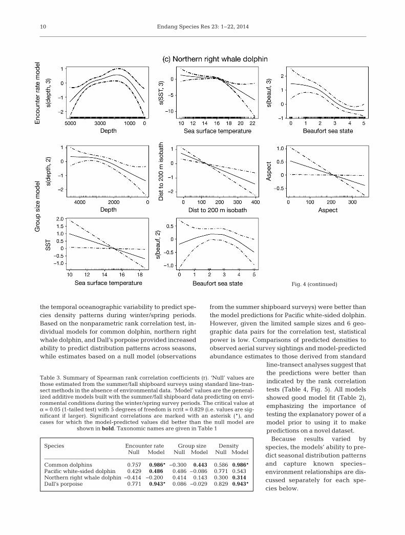
shipboard data were similar to those observed in pre-vious studies (Table 1, Fig. 4; Barlow et al. 2009,Becker et al. 2010, 2012b, Forney et al. 2012). En -counters with common dolphin were highest in thewarmest waters in the study area, with encountersdropping substantially in water temperatures belowabout 16°C (Fig. 4a). A bimodal depth distributionwas evident in the encounter rate GAM for commondolphin, with fewest encounters in waters approxi-mately 2000 to 3000 m deep. The encounter ratemodels for Pacific white-sided dolphin and northernright whale dolphin were similar, both showing highest encounters in cooler waters over the conti-nental shelf and slope, with a substantial drop inencounters in water temperatures greater than about16°C (Fig. 4b,c). Highest encounters of Dall’s por-poise occurred in cool northern shelf and slopewaters, with encounters dropping substantially inwater temperatures greater than approximately 17°C(Fig. 4d).

The percentage of deviance explained by both theencounter rate and group size models was similar toprevious studies (Barlow et al. 2009, Becker et al.2010, 2012b, Forney et al. 2012). The percentage ofdeviance explained by the encounter rate modelsranged from 15% (northern right whale dolphin) to34% (Dall’s porpoise) and from 2% (common dol-phins) to 30% (northern right whale dolphin) for thegroup size models (Table 2). Ratios of observed topredicted abundance summarized over all years forthe entire study area indicate that the summer mod-els accurately predicted the abundance of these 4species during the summer season, as all ratios werewithin 3% of unity (Table 2).

Across-season predictive ability of summer models

Rank correlation tests

Despite the relatively high percentage of explaineddeviance for the Pacific white-sided dolphin andnorthern right whale dolphin group size models (29and 30%, respectively), they were not effective atpredicting spatial variability in group size during thewinter, as indicated by the rank correlation test(Table 3). Conversely, the encounter rate model pre-dictions for all species except northern right whaledolphin were better than the null model, and this dif-ference was significant (p < 0.05) for both commondolphins and Dall’s porpoise.

The summer models’ ability to predict winter den-sities across geographic strata exceeded that of the

7

Endang Species Res 23: 1–22, 2014

null model for 3 of the 4 taxa (common dolphins,northern right whale dolphin, and Dall’s porpoise).For both the common dolphin and Dall’s porpoisemodels, their ability to effectively predict spatial den-sity patterns in winter was significantly better thanthe null model (p < 0.05; Table 3).

Visual inspection of density plots

Visual comparisons of predicted winter densitiesversus observed sightings from the aerial surveyssuggest that the predictions were better than indi-cated by the coarse-scale rank correlation tests, as

8

Species Model GAM

Common dolphins ER s(depth, 3) + s(slope, 2) + dist200 + s(aspect, 3) + s(SST, 3) + s(beauf, 3) + offsetDelphinus spp. GS s(depth, 3)

Pacific white-sided dolphin ER s(depth, 3) + dist200 + s(SST, 3) + s(beauf, 3) + offsetLagenorhynchus obliquidens GS s(depth, 3) + dist200 + s(beauf, 3)

Northern right whale dolphin ER s(depth, 3) + s(SST, 3) + s(beauf, 3) + offsetLissodelphis borealis GS s(depth, 2) + dist200 + aspect + SST + s(beauf, 2)

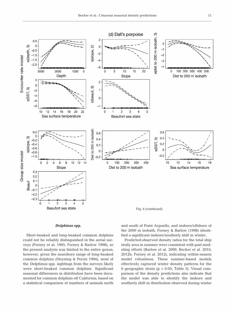
Dall’s porpoise Phocoenoides dalli ER s(depth, 3) + s(slope, 2) + s(dist200, 3) + s(SST, 3) + s(beauf, 3) + offset GS s(slope, 3) + dist200 + s(SST, 3) + beauf

Table 1. Predictor variables included in the final encounter rate (ER) and group size (GS) models for the 1991 to 2008 summer/fallsurvey data. The expression s(x,n) indicates a non-parametric smoothing spline of the variable x with n degrees of freedom.GAM: generalized additive model, SST: sea surface temperature, depth: water depth, slope: bathymetric slope, aspect: slope aspect, dist200: distance to the 200 m isobath, beauf: Beaufort sea state, offset: offset[ln(effective distance searched in km)]

Fig. 4. Encounter rate and group size model functions for (a) common dolphins,(b) Pacific white-sided dolphin, (c) northern right whale dolphin, and (d) Dall’sporpoise (for taxonomic names see Table 1). Models were constructed with bothlinear terms and smoothing splines having up to 3 degrees of freedom. Degreesof freedom for nonlinear fits are in parentheses on the y-axes. Potential predictorvariables included sea surface temperature (SST, °C), water depth (depth, m),bathymetric slope (slope, °), slope aspect (aspect, slope direction in °), distance tothe 200 m isobath (dist to 200 m isobath, m), and Beaufort sea state (beauf).Hatch marks on the x-axes show samples. The y-axes represent the term’s (lin-ear or spline) function. Zero on the y-axes corresponds to no effect of the predic-tor variable on the estimated response variable (encounter rate or group size).Scaling of y-axis varies among predictor variables to emphasize model fit. Thedashed lines reflect 2× standard error bands (i.e. 95% confidence interval)

Becker et al.: Cetacean seasonal density predictions

shifts in distribution were captured for all 4 taxa(Fig. 5). Further, for all but northern right whaledolphin, the winter predictions fell largely withinthe 90% confidence interval (as derived frominterannual variability in summer density patterns)of the predictions based on the summer data, sug-gesting that interannual variability is comparableto seasonal variability for the remaining 3 taxa(Fig. 6).

Observed:predicted abundance estimates

Winter abundance estimates predicted by the sum-mer habitat models fell within the 95% con fidenceintervals of the standard line-transect analysis of thewinter aerial survey data for all species except north-ern right whale dolphin, for which the modeledabundance estimate was more than 3 times higherthan the line-transect point estimate (Table 4). Themodeled abundance estimate for Dall’s porpoise wasvery similar to that derived using standard line- transect analyses, while the modeled abundance es-timates for Pacific white-sided dolphin and commondolphins were lower than the line-transect derivedestimates, and for the latter genus substantially so(almost half; Table 4).

DISCUSSION

In this study we evaluated whether summer/fallhabitat-based density models developed based onmultiple years of survey data can capture enough of

9

Species Explained deviance Obs/Encounter Group predrate model size model

Common dolphins 15.5 2.1 0.97Pacific white-sided dolphin 23.5 29.1 0.98Northern right whale dolphin 14.8 29.7 1.01Dall’s porpoise 33.7 10.8 1.00

Table 2. Percentage of deviance explained by the 1991−2008encounter rate and group size models for each species, and theratio of the observed to model-predicted study area density esti-mates for the summer/fall shipboard surveys (Obs/pred). Taxo-

nomic names are given in Table 1

Fig. 4 (continued)

Endang Species Res 23: 1–22, 2014

the temporal oceanographic variability to predict spe-cies density patterns during winter/spring periods.Based on the nonparametric rank correlation test, in-dividual models for common dolphin, northern rightwhale dolphin, and Dall’s porpoise provided increasedability to predict distribution patterns across seasons,while estimates based on a null model (observations

from the summer shipboard surveys) were better thanthe model predictions for Pacific white-sided dolphin.However, given the limited sample sizes and 6 geo-graphic data pairs for the correlation test, statisticalpower is low. Comparisons of predicted densities toobserved aerial survey sightings and model-predictedabundance estimates to those derived from standard

line-transect analyses suggest thatthe predictions were better thanindicated by the rank correlationtests (Table 4, Fig. 5). All modelsshowed good model fit (Table 2),emphasizing the importance oftesting the ex planatory power of amodel prior to using it to makepredictions on a novel dataset.

Because results varied by species, the models’ ability to pre-dict seasonal distribution patternsand capture known species−environment relationships are dis -cussed separately for each spe-cies below.

10

Species Encounter rate Group size DensityNull Model Null Model Null Model

Common dolphins 0.757 0.986* −0.300 0.443 0.586 0.986*Pacific white-sided dolphin 0.429 0.486 0.486 –0.086 0.771 0.543Northern right whale dolphin −0.414 −0.200 0.414 0.143 0.300 0.314Dall’s porpoise 0.771 0.943* 0.086 −0.029 0.829 0.943*

Table 3. Summary of Spearman rank correlation coefficients (r). ‘Null’ values arethose estimated from the summer/fall shipboard surveys using standard line-tran-sect methods in the absence of environmental data. ‘Model’ values are the general-ized additive models built with the summer/fall shipboard data predicting on envi-ronmental conditions during the winter/spring survey periods. The critical value atα = 0.05 (1-tailed test) with 5 degrees of freedom is rcrit = 0.829 (i.e. values are sig-nificant if larger). Significant correlations are marked with an asterisk (*), andcases for which the model-predicted values did better than the null model are

shown in bold. Taxonomic names are given in Table 1

Fig. 4 (continued)

Becker et al.: Cetacean seasonal density predictions

Delphinus spp.

Short-beaked and long-beaked common dolphinscould not be reliably distinguished in the aerial sur-veys (Forney et al. 1995, Forney & Barlow 1998), sothe present analysis was limited to the entire genus;however, given the nearshore range of long-beakedcommon dolphins (Heyning & Perrin 1994), most ofthe Delphinus spp. sightings from the surveys likelywere short-beaked common dolphins. Significantseasonal differences in distribution have been docu-mented for common dolphins off California; based ona statistical comparison of numbers of animals north

and south of Point Arguello, and inshore/offshore ofthe 2000 m isobath, Forney & Barlow (1998) identi-fied a significant inshore/southerly shift in winter.

Predicted:observed density ratios for the total shipstudy area in summer were consistent with past mod-eling efforts (Barlow et al. 2009, Becker et al. 2010,2012b, Forney et al. 2012), indicating within-seasonmodel robustness. These summer-based modelseffectively captured winter density patterns for the6 geographic strata (p < 0.05; Table 3). Visual com-parison of the density predictions also indicate thatthe model was able to identify the inshore andsoutherly shift in distribution observed during winter

11

Fig. 4 (continued)

Endang Species Res 23: 1–22, 2014

1991/92, and the model predictions were notably different than those for summer, when Delphinusspp. were predicted well north of Point Arguelloand farther offshore (Fig. 5a).

The study area abundance of common dolphinsduring winter, as estimated from model predictions,was about half of that derived from standard line-transect analyses but well within the line-transect

12

Fig. 5. Predicted densities from the summer/fall shipboard models based on summer/fall environmental data used for modelbuilding (left panels) and winter/spring environmental data (right panels), for (a) common dolphins, (b) Pacific white-sideddolphin, (c) northern right whale dolphin, and (d) Dall’s porpoise. Predictions are shown for the study area (ship survey studyarea in left panels and aerial survey study area in right panels). Interpolation grids were created at a resolution of 25 km, usinginverse distance weighting to the second power in Surfer software (Version 9). The light gray line west and offshore of the aer-ial study area (right panels) marks the extent of the shipboard study area. Red (blue) represents highest (lowest) predicteddensity, as shown in the species-specific density keys. Black dots show actual sighting locations for the summer/fall ship sur-veys (left panels) and winter/spring aerial surveys (right panels), with larger dots representing more animals per surveyed

segment (Obs. Seg. Density). For taxonomic names see Table 1

Becker et al.: Cetacean seasonal density predictions

confidence limit (Table 4). Common dolphins typicallyoccur in large groups, and availability bias is expectedto be relatively small for the aerial surveys, but thiswould further increase the difference be tween themodel- and survey-estimated values. The winteraerial surveys were conducted in 1991/92 during anEl Niño year, when water temperatures off SouthernCalifornia were anomalously high (Hayward 1993).Short-beaked common dolphins are a warm temper-ate to tropical species, and based on the models de-

veloped here as well as in previous studies (Barlow etal. 2009, Becker et al. 2010, 2012b, Forney et al. 2012),densities are greatest when waters are warmest(Figs. 4a & 5a). It is probable that there was a large in-flux of common dolphins into the study area in winterof 1991/92. The difference in abundance between themodel estimate and the line-transect estimate couldbe caused by uncertainty in both estimates (withinconfidence limits), or it could be related to a potentialEl Niño-related influx of animals.

13

Fig. 5 (continued)

Endang Species Res 23: 1–22, 2014

The northern extent of short-beaked common dol-phin distribution off the US west coast varies on aninterannual basis but is generally south of 45° N lat-itude (Smith et al. 1986, Forney & Barlow 1998,

Hamilton et al. 2009). Interestingly, the averagedensity predictions for summer showed an area ofmoderate density along the coast at approximately45° N latitude (Fig. 5a), where, other than strandings

14

Fig. 6. Standard deviation (SD(Dens)), and upper and lower lognormal 90% confidence limits (Lo90% and Hi90%) based onthe summer/fall models predicted on summer environmental data, and winter/spring density predictions for: (a) common dol-phins, (b) Pacific white-sided dolphin, (c) northern right whale dolphin, and (d) Dall’s porpoise. Predicted values for each sur-vey year were interpolated using inverse distance weighting (see ‘Methods’ for details). Grid cells for each of the individualsurvey years were then averaged across all years and SD and upper and lower lognormal 90% confidence limits were calcu-lated from the grid cell averages and variances using standard formulae. The light gray line marks the extent of the shipboardstudy area. Red (blue) represents highest (lowest) predicted density, as shown in the species-specific density keys. The densityscale for the winter predictions has been scaled relative to the 90% confidence limits. For taxonomic names see Table 1

Becker et al.: Cetacean seasonal density predictions

and occasional sightings, this species has not previ-ously been documented (Barlow et al. 2009, Hamil-ton et al. 2009, Barlow 2010, Becker et al. 2012b,Forney et al. 2012). One group of approximately 40short-beaked common dolphins was sighted offnorthern Washington at about 48° N latitude in 2005(Forney 2007), but this was considered unusual.Short-beaked common dolphins are the most abun-

dant cetacean species off the US west coast (Barlow2010), and their distribution shifts with changingoceanic conditions (Barlow et al. 2009, Becker et al.2012b, Forney et al. 2012), but insufficient data arecurrently available to resolve whether this higher-density region identified by this summer model near45° N has a biological basis or indicates potentialmis-specification of the model.

15

Fig. 6 (continued)

Endang Species Res 23: 1–22, 2014

Pacific white-sided dolphin

Based on morphological and genetic evidence, 2forms of Pacific white-sided dolphin occur in watersoff California (Walker et al. 1986, Lux et al. 1997);however, they currently cannot be reliably distin-guished in the field and are therefore treatedtogether in the present analysis. Survey data indi-cate that the seasonal distribution of Pacific white-sided dolphins off the US west coast varies dramati-

cally, as animals move north into waters off Oregonand Washington during the summer months andsouth into southern California waters during thewinter months (Green et al. 1992, Forney & Barlow1998).

The stratum-specific modeled densities for Pacificwhite-sided dolphin failed to effectively predictwinter density patterns as indicated by the rankcorrelation tests (Table 3). Visual inspection of thedensity plots for this species suggest that the mod-

16

Fig. 6 (continued)

els’ predictive ability was better than indicated,however, because greater densities were predictedsouth of about 33° N latitude, where large numbersof Pacific white-sided dolphins were sighted duringthe 1991/ 92 aerial surveys (Fig. 5b). Further, com-pared to the predicted density patterns in summer,a clear southerly shift in distribution is evident inthe winter plot, indicating that the summer-basedmodels more closely match the observed winterpatterns.

The estimated winter abundance of Pacific white-sided dolphins based on model predictions was similarto (within 12% of) the estimate de rived from standardline-transect analyses (Table 4). A higher proportion ofanimals is expected to be missed during aerial surveysdue to availability bias, so the actual difference may begreater than indicated; however, Pacific white-sideddolphins commonly occur in large, asynchronouslydiving groups, so the magnitude of the aerial surveyavailability bias is expected to be small.

Becker et al.: Cetacean seasonal density predictions 17

Fig. 6 (continued)

Endang Species Res 23: 1–22, 2014

Northern right whale dolphin

Northern right whale dolphin is a cold-temperatespecies whose distribution shifts south into shelf wa-ters of the Southern California Bight in the winterwhen waters are relatively cool (Dohl et al. 1978,Leatherwood & Walker 1979, Forney & Barlow 1998).Based on the stratum-specific density estimates, themodel predictions were slightly better than those ofthe null model (Table 3), and visual inspection of thedensity plots for this species indicate that the modelcaptured the winter distribution shift into shelf watersof the Southern California Bight (Fig. 5c). However,both the spatial range and absolute values of the win-ter density predictions extend outside the upper 90%confidence interval of the summer model in 2 regions:(1) in the Southern California Bight to the south andsouthwest of 34° N, and (2) north and northwest of39° N where the winter plot suggests that the model isoverpredicting density (Fig. 6c). This indicates thatthe range of interannual variability in oceanic condi-tions encompassed by the summer-based models didnot adequately capture winter conditions, particularlyfor SST, which was a predictor in both the encounterrate and group size GAMs for northern right whaledolphin. Encounter rates and group sizes were pre-dicted to be greatest within the coolest waters in thestudy area in summer (Fig. 3c); however, during sum-mer the SST values ranged from 9.9 to 22.4°C, whilewinter SSTs ranged from 8.7 to 17.1°C. The modelpredictions for SSTs below the range of values ob-served during summer caused unreliable estimatesfor winter cool water conditions. This result highlightsthe need to avoid predicting out of the bounds of thevariables used for model development.

Forney & Barlow (1998) identified a statistically sig-nificant difference in the abundance of northern rightwhale dolphin between summer and winter survey

periods off California, with more ani-mals present during the cold water pe-riod. The estimated winter abundanceof northern right whale dolphin basedon model predictions was almost 3times higher than the estimate derivedfrom standard line-transect analyses,and well above the upper 95% confi-dence interval (Table 4). A higher pro-portion of animals is expected to bemissed during the aerial surveys due toavailability bias; however, it is unlikelythat the magnitude of this bias wouldbe large enough to account for the dif-ference in model-predicted versus line-

transect-derived density estimates. The overestimateis likely the result of the models predicting outside therange of values used to build them as noted above. Insummary, while the models exhibited some ability topredict seasonal shifts in distribution, more data col-lected over a range of oceanic conditions are neededto make the models robust and allow them to more ac-curately predict absolute abundance throughout thestudy area.

Dall’s porpoise

Previous analyses of a portion of the cetaceansighting data used for this study found a statisticallysignificant seasonal difference in the distribution ofDall’s porpoise north and south of Point Arguello,documenting a southward shift during winter (For-ney & Barlow 1998). The summer model’s ability tocapture the seasonal distribution shift was significant(p < 0.05) as indicated by the rank correlation test(Table 3). Visual comparison of the density predic-tions also indicate that the model was able to identifythe southerly shift in distribution observed duringwinter 1991/92. Dall’s porpoise was predicted tooccur well south of Point Arguello, consistent withthe winter survey sightings and notably differentthan the summer distribution pattern in the SouthernCalifornia Bight (Fig. 5d).

The model-predicted abundance estimate for thewinter study area was very similar to that derivedfrom standard line-transect analyses, and well withinthe 95% confidence interval of the latter (Table 4).Availability bias was accounted for in the line-tran-sect abundance estimate for Dall’s porpoise (Forney& Barlow 1998), and this may have contributed to thesimilarity in estimates derived from the summermodel predictions.

18

Species Winter abundance Line-transectestimates bootstrap CIs

Model Line-transect L95% U95%

Common dolphins 156010 305694 124493 541163Pacific white-sided dolphin 108338 121693 35625 261931Northern right whale dolphin 66875 21332 9902 46147Dall’s porpoise 21841 26111 14919 46201

Table 4. Modeled abundance estimates (Model) and those derived from survey observations by Forney et al. (1995) using standard line-transect analy-ses (line-transect). Bootstrap confidence intervals (CIs, shown with lower andupper 95th percentiles) were recalculated from the original line-transect datausing the BCa method (Efron & Tibshirani 1993). Taxonomic names are given

in Table 1

Becker et al.: Cetacean seasonal density predictions

Seasonal predictions

In many regions with clearly distinctive seasonaldifferences (e.g. polar regions), it would not beappropriate to use models built with summer datain an attempt to make winter predictions. Across- season predictions also are not appropriate for highlymigratory species, e.g. many baleen whales that areknown to be absent from the study area during oneseason and present in another, unless this migratorypattern is included in the model. Social organizationand behavioral aspects of species ecology may alsoconfound the cetacean−habitat modeling approach,particularly when attempting to predict across sea-sons. In addition, anthropogenic activity may deteranimals from preferred habitat, further confoundingpredictions from habitat models. For species presentin an area year-round and known to have pro-nounced seasonal distribution shifts, the results ofthis study indicate that spatially explicit habitat mod-els can be valuable tools for assessing species distri-butions in a temporally dynamic environment, al -though model accuracy is directly related to thedegree to which the models can capture year-roundhabitat conditions.

A notable difference between our study and an ini-tial evaluation of across-season predictive abilityusing a subset of these data (Becker 2007) was thenumber of sightings available to build and evaluatethe models. The initial analysis relied on SST satellitedata measured from passive infrared sensors (e.g.Pathfinder), which creates data gaps due to cloudcover. In the present study we used a more recentsatellite-derived SST product that blends in situ andinfrared sensor measurements and virtually eliminatesdata gaps due to cloud cover (Reynolds et al. 2007).On a species-specific basis, this increased the numberof summer ship survey sightings available to build themodels by up to 54% for the years included in the ini-tial study (1991 to 2001) and increased the number ofwinter aerial survey sightings used to evaluate thepredictions by up to 30%. Further, the present studyincluded 2 additional years of ship survey data (2005and 2008) and expanded the study area north to in-clude waters off Oregon and Washington, thus includ-ing a broader range of environmental conditions formodel development. These improvements resulted inmore robust models, as demonstrated by the increasedexplanatory and predictive power of the models.

SST was the only dynamic environmental predictorvariable included in the models used in the presentstudy. Remotely sensed measures of chlorophyllcould not be included because they were not avail-

able during 1991 to 1996, and satellite-derived salin-ity measurements have only been available since2011. Further improvements to across-season predic-tions may be realized with the inclusion of additionalenvironmental variables, particularly those that pro-vide a more direct link to cetacean prey, such as zoo-plankton indices currently available from in situ data(Redfern et al. 2008, Barlow et al. 2009). Although theuse of such predictors may improve model perform-ance, collecting and processing in situ oceanographicdata requires substantial time and expense, and pre-dictive models that rely on in situ data may not be asuseful to resource managers who are often requiredto make timely decisions related to protected speciesabundance and distribution. For cetacean speciesthat require more complex habitat models thatinclude predictor variables such as mixed layer depthand prey indices (Redfern et al. 2008, Barlow et al.2009, Becker et al. 2012b, Forney et al. 2012), nearreal-time and forecast predictions from ocean circu-lation models (e.g. Chao et al. 2009) may provide ameans to improve across-season predictions.

Methodology

Differences in species distribution may arise fromvariability in the number of groups in a given area orvariability in group size, with potentially different en-vironmental factors affecting the 2 parameters. To ac-count for these differences, density estimates are typi-cally derived from separate encounter rate and groupsize models using appropriate statistical distributions(Ferguson et al. 2006, Redfern et al. 2008, Barlow et al.2009, Becker et al. 2010, 2012a,b, Forney et al. 2012).For species that typically occur in small groups (e.g.some baleen whales), the number of individual ani-mals can be modeled as a single response variable(e.g. Redfern et al. 2013). Large variability in groupsize is evident for the delphinids addressed in thisstudy, and hence we developed separate group sizemodels. However, the lack of success in predictinggroup size in this and other studies (e.g. Ferguson etal. 2006, Redfern et al. 2008) suggests that either weare not including the appropriate environmental vari-ables in our models or there are other non-environ-mental variables determining group size (e.g. socialorganization, predator protection, behavioral aspects;Reilly & Fiedler 1994). Future studies should evaluatealternative sampling distributions for modeling en-counter rate and group size as a single response vari-able for species with large group size variability in or-der to better capture spatial patterns.

19

Endang Species Res 23: 1–22, 2014

Implications for marine spatial planning

Effective pelagic conservation planning requiresbroad-scale information on species density acrossspace and time, but management is often limited bythe lack of data. This study was designed to evaluatethe extent to which cross-season predictions might bevalid within the CCE, a temporally dynamic environ-ment. Results suggest that, although the processes ofinterannual and seasonal variability are different, in-terannual variability in the environmental parameterscan be large enough to explain some of the variationin the seasonal distribution patterns of cetaceans inthe waters off California. More importantly, modelsneed to be developed using environmental parame-ters that include the full range of conditions for thetemporal/spatial period they are predicting.

Ideally, cetacean survey data would be collectedfor the specific time period of interest and spatialhabitat models built accordingly. However, in mostareas cetacean survey data are biased towards sum-mer (Kot et al. 2010). In the absence of actual surveydata, results suggest that the seasonal geographicpatterns of species density were captured effectivelyfor most species, and demonstrate that there is poten-tial to improve our decision-making through suchmodels, but limitations and caveats must be consid-ered. In this case, for marine planning activities thatrequire an understanding of winter species distribu-tion in order to assess and minimize potential im -pacts, the across-season predictions are more inform-ative than the complete absence of data or thereliance on summer distribution patterns. In termsof estimating the total number of animals potentiallyexposed to a given anthropogenic activity, themodel-derived density estimates would need to beapplied cautiously on a species-by-species basis,with the recognition that in some cases the out-of-bound predictions could produce unrealistic results.For example, since the linear SST function in thegroup size model for northern right whale dolphinscontributed to overpredictions of winter densities, aconstant group size estimate could be used in concertwith the encounter rate model to eliminate this effecton the density estimates. With the recognition ofmodel limits, habitat-based density models can bevaluable tools for assessing species distributions andinforming pelagic management decisions.

Acknowledgements. We thank everyone who spent longhours collecting the data used in our analyses, including themarine mammal observers, cruise leaders, officers, and crewof the RV ‘David Starr Jordan,’ RV ‘McArthur,’ and RV

‘McArthur II,’ as well as the marine mammal observers, datarecorders, and pilots responsible for the 1991/92 aerial sur-veys. Chief Scientists for the ship survey cruises included T.Gerrodette and 2 of the co-authors (J.B. and K.A.F.). Thispaper was improved by reviews from S. Benson, J. Carretta,A. Dransfield, and 1 anonymous referee. Special thanks to J.Michaelsen, J. Richardson, and L. Washburn for their con-structive comments on earlier versions of this manuscript.Funding for this project was provided by the Strategic Envi-ronmental Research and Development Program (SERDP),under Conservation Project CS-1391, and the SouthwestFisheries Science Center.

LITERATURE CITED

Akaike H (1973) Information theory and an extension of themaximum likelihood principle. In: Petran BN and CsàakiF (eds) 2nd Int Symp Inf Theory. Akadèemiai Kiadi,Budapest, p 267−281

Amante C, Eakins BW (2009) ETOPO1 1 arc-minute globalrelief model: procedures, data sources and analysis. TechMemo NESDIS NGDC-24. National Geophysical DataCenter, Boulder, CO

Barber RT, Chavez FP (1983) Biological consequences of ElNiño. Science 222: 1203−1210

Barber RT, Smith RL (1981) Coastal upwelling ecosystems.In: Longhurst AR (ed) Analysis of marine ecosystems.Academic Press, New York, NY, p 31−68

Barlow J (2003) Preliminary estimates of the abundance ofcetaceans along the U.S. west coast: 1991-2001. NOAAAdmin Rep LJ-03-03. Southwest Fisheries Science Cen-ter, National Marine Fisheries Service, La Jolla, CA

Barlow J (2010) Cetacean abundance in the California Current estimated from a 2008 ship-based line-transectsurvey. NOAA Tech Memo NMFS-SWFSC-456

Barlow J, Forney KA (2007) Abundance and density ofcetaceans in the California Current ecosystem. Fish Bull105: 509−526

Barlow J, Gerrodette T, Forcada J (2001) Factors affectingperpendicular sighting distances on shipboard line-tran-sect surveys for cetaceans. J Cetacean Res Manag 3: 201−212

Barlow J, Ferguson MC, Becker EA, Redfern JV and others(2009) Predictive modeling of cetacean densities inthe eastern Pacific Ocean. NOAA Tech Memo NMFS-SWFSC-444

Barlow J, Calambokidis J, Falcone EA, Baker CS and others(2011) Humpback whale abundance in the North Pacificestimated by photographic capture-recapture with biascorrection from simulation studies. Mar Mamm Sci 27: 793−818

Becker EA (2007) Predicting seasonal patterns of Californiacetacean density based on remotely sensed environmen-tal data. PhD dissertation, University of California, SantaBarbara, CA

Becker EA, Forney KA, Ferguson MC, Foley DG, Smith RC,Barlow J, Redfern JV (2010) Comparing California Cur-rent cetacean−habitat models developed using in situand remotely sensed sea surface temperature data. MarEcol Prog Ser 413: 163−183

Becker EA, Foley DG, Forney KA, Barlow J, Redfern JV,Gentemann CL (2012a) Forecasting cetacean abundancepatterns to enhance management decisions. EndangSpecies Res 16: 97−112

20

Becker et al.: Cetacean seasonal density predictions

Becker EA, Forney KA, Ferguson MC, Barlow J, Redfern JV(2012b) Predictive modeling of cetacean densities inthe California Current ecosystem based on summer/fallship surveys in 1991-2008. NOAA Tech Memo NMFS-SWFSC-499

Briggs JC (1974) Marine zoography. McGraw-Hill, NewYork, NY

Buckland ST, Anderson DR, Burnham KP, Laake JL,Borchers DL, Thomas L (2001) Introduction to distancesampling: estimating abundance of biological popula-tions. Oxford University Press, Oxford

Calambokidis J, Steiger GH, Rasmussen K, Urban J and oth-ers (2000) Migratory destinations of humpback whalesthat feed off California, Oregon and Washington. MarEcol Prog Ser 192: 295−304

Calambokidis J, Barlow J, Ford KB, Chandler TE, DouglasAB (2009) Insights into the population structure of bluewhales in the eastern North Pacific from recent sightingsand photographic identifications. Mar Mamm Sci 25: 816−832

Cañadas A, Sagarminaga R, García-Tiscar S (2002) Ce -tacean distribution related with depth and slope in theMediterranean waters off southern Spain. Deep-Sea ResI 49: 2053−2073

Carretta JV, Forney KA (1993) Report of the two aerial sur-veys for marine mammals in California waters utilizing aNOAA DeHavilland Twin Otter aircraft, March 9-April 7,1991 and February 8-April 6, 1992. NOAA Tech MemoNOAA-TM-NMFS-SWFSC-185

Chao Y, Li Z, Farrara J, McWilliams JC and others (2009)Development, implementation and evaluation of a data-assimilative ocean forecasting system off the central Cal-ifornia coast. Deep-Sea Res II 56: 100−126

Chavez FP, Ryan J, Lluch-Cota SE, Niquen CM (2003) Fromanchovies to sardines and back: multidecadal change inthe Pacific Ocean. Science 299: 217−221

Dohl TP, Norris KS, Guess RC, Bryant JD, Honig MW (1978)Summary of marine mammal and seabird surveys of theSouthern California Bight area, 1975-78, Vol III: investi-gators’ reports, Part II: Cetacea of the Southern Califor-nia Bight. Final Report to the Bureau of Land Manage-ment, NTIS Catalog No. PB81-248189. University ofCalifornia, Santa Cruz, CA

Dohl TP, Guess RC, Duman ML, Helm RC (1983) Cetaceansof central and northern California, 1980−1983: status,abundance, and distribution. Prepared for Pacific OCSRegion, Minerals Management Service, U.S. Departmentof the Interior. Contract No. 14-12-0001-29090, NTISCatalog No. PB85-183861. Pacific OCS Region, MineralsManagement Service, US Dept. of the Interior, Los Ange-les, CA

Dohl TP, Bonnell ML, Ford RG (1986) Distribution and abun-dance of common dolphin, Delphinus delphis, in theSouthern California Bight: a quantitative assessmentbased upon aerial transect data. Fish Bull 84: 333−343

Doyle RF (1985) Biogeographical studies of rocky shore nearPoint Conception, California. PhD dissertation, Univer-sity of California, Santa Barbara, CA

Edwards EF, Perkins PC (1992) Power to detect linear trendsin dolphin abundance: estimates from tuna-vessel ob -server data, 1975-89. Fish Bull 90: 625−631

Efron B, Tibshirani RJ (1993) An introduction to the boot-strap. Chapman and Hall, London

Ferguson MC, Barlow J, Fiedler P, Reilly SB, Gerrodette T(2006) Spatial models of delphinid (family Delphinidae)

encounter rate and group size in the eastern tropicalPacific Ocean. Ecol Model 193: 645−662

Forney KA (1999) Trends in harbor porpoise abundance offcentral California, 1986-95; evidence for interannualchange in distribution? J Cetacean Res Manag 1: 73−80

Forney KA (2000) Environmental models of cetacean abun-dance: reducing uncertainty in population trends. Con-serv Biol 14: 1271−1286

Forney KA (2007) Preliminary estimates of cetacean abun-dance along the U.S. west coast and within four NationalMarine Sanctuaries during 2005. NOAA Tech MemoNMFS-SWFSC-406

Forney KA, Barlow J (1998) Seasonal patterns in the abun-dance and distribution of California cetaceans, 1991-1992. Mar Mamm Sci 14: 460−489

Forney KA, Hanan DA, Barlow J (1991) Detecting trends inharbor porpoise abundance from aerial surveys usinganalysis of covariance. Fish Bull 89: 367−377

Forney KA, Barlow J, Carretta JV (1995) The abundance ofcetaceans in California waters. Part II: aerial surveys inwinter and spring of 1991 and 1992. Fish Bull 93: 15−26

Forney KA, Ferguson MC, Becker EA, Fiedler PC and others(2012) Habitat-based spatial models of cetacean densityin the eastern Pacific Ocean. Endang Species Res 16: 113−133

Gerrodette T, Eguchi T (2011) Precautionary design of amarine protected area based on a habitat model. EndangSpecies Res 15: 159−166

Gilles A, Adler S, Kaschner K, Scheidat M, Siebert U (2011)Modelling harbour porpoise seasonal density as a func-tion of the German Bight environment: implications formanagement. Endang Species Res 14: 157−169

Goetz KT, Montgomery RA, Ver Hoef JM, Hobbs RC, John-son DS (2012) Identifying essential summer habitat of theendangered beluga whale Delphinapterus leucas inCook Inlet, Alaska. Endang Species Res 16: 135−147

Green GA, Brueggeman JJ, Grotefendt RA, Bowlby CE,Bonnell ML, Balcomb KC III (1992) Cetacean distributionand abundance off Oregon and Washington, 1989-1990.In: Oregon and Washington marine mammal and seabirdsurveys. In: Brueggeman JJ (ed) OCS Study MMS 91-0093, contract 14-12-0001-30426. U.S. Department of theInterior, Minerals Management Service, Los Angeles,CA, p 1−100

Green GA, Grotefendt RA, Smultea MA, Bowlby CE,Rowlett RA (1993) Delphinid aerial surveys in Oregonand Washington offshore waters. Contract No. 50 ABNF -200058. Final report prepared for NMFS. National Mar-ine Mammal Lab, Alaska Fisheries Science Center, Seat-tle, WA

Hamilton TA, Redfern JV, Barlow J, Ballance LT and others(2009) Atlas of cetacean sightings for Southwest Fish-eries Science Center cetacean and ecosystem surveys: 1986-2005. NOAA Tech Memo NMFS-SWFSC-440

Hastie TJ, Tibshirani RJ (1990) Generalized additive mod-els, Vol 43. Chapman & Hall/CRC, Boca Raton, FL

Hayward TL (1993) Preliminary observations of the 1991-1992 El Niño in the California Current. Calif Coop OceanFish Invest Rep 34: 21−29

Heyning JE, Perrin WF (1994) Evidence for two species ofcommon dolphin (genus Delphinus) from the easternNorth Pacific. Los Angel Cty Mus Nat Hist Contrib Sci442: 1−35

Hickey BM (1979) The California Current System—hypo -theses and facts. Prog Oceanogr 8: 191−279

21

Endang Species Res 23: 1–22, 2014

Hooker SK, Whitehead H, Gowans S (1999) Marine pro-tected area design and the spatial and temporal distribu-tion of cetaceans in a submarine canyon. Conserv Biol13: 592−602

Kaschner K, Watson R, Trites AW, Pauly D (2006) Mappingworld-wide distributions of marine mammal speciesusing a relative environmental suitability (RES) model.Mar Ecol Prog Ser 316: 285−310

Keller CA, Garrison L, Baumstark R, Ward-Geiger LI, HinesE (2012) Application of a habitat model to define calvinghabitat of the North Atlantic right whale in the southeast-ern United States. Endang Species Res 18: 73−87

Kinzey D, Olson P, Gerrodette T (2000) Marine mammaldata collection procedures on research ship line-transectsurveys by the Southwest Fisheries Science Center.Report No. LJ-00-08. Southwest Fisheries Science Cen-ter, La Jolla, CA

Koslow JA, Hobday AJ, Boehlert GW (2002) Climate vari-ability and marine survival of coho salmon (Oncorhyn-chus kisutch) in the Oregon production area. FishOceanogr 11: 65−77

Kot CY, Fujioka E, Hazen LJ, Best BD, Read AJ, Halpin PN(2010) Spatio-temporal gap analysis of OBIS-SEAMAPproject data: assessment and way forward. PLoS ONE 5: e12990

Leatherwood S, Walker WA (1979) The northern right whaledolphin Lissodelphis borealis Peale in the eastern NorthPacific. In: Winn HE, Olla BL (eds) Behavior of marineanimals, Vol 3: cetaceans. Plenum Press, New York, NY,p 85−141

Lux CA, Costa AS, Dizon AE (1997) Mitochondrial DNApopulation structure of the Pacific white-sided dolphin.Rep Int Whal Comm 47: 645−652

Lynn RJ, Simpson JJ (1987) The California Current system: the seasonal variability of its physical characteristics. JGeophys Res 92: 12947−12966, doi: 10. 1029/ JC 092iC 12 p12947

Mantua NJ, Hare SR (2002) The Pacific Decadal Oscillation.J Oceanogr 58: 35−44

Maravelias CD, Reid DG, Swartzman G (2000) Modellingspatio-temporal effects of environment on Atlanticherring, Clupea harengus. Environ Biol Fishes 58: 157−172

Marsh H, Sinclair DF (1989) Correcting for visibility bias instrip transect aerial surveys of aquatic fauna. J WildlManag 53: 1017−1024

McGowan JA, Cayan DR, Dorman LM (1998) Climate-oceanvariability and ecosystem response in the NortheastPacific. Science 281: 210−216

Newman WA (1979) California transition zone: significanceof short-range endemics. In: Gray J, Boucot AJ (eds) His-torical biogeography, plate tectonics, and the changingenvironment. Oregon State University Press, Corvallis,OR, p 399−416

Palacios DM, Bograd SJ, Foley DG, Schwing FB (2006)Oceanographic characteristics of biological hot spots inthe North Pacific: a remote sensing perspective. Deep-Sea Res II 53: 250−269

Peterman RM, Bradford MJ (1987) Statistical power oftrends in fish abundance. Can J Fish Aquat Sci 44: 1879−1889

Pyper BJ, Peterman RM (1999) Relationship among adult

body length, abundance, and ocean temperature forBritish Columbia and Alaska sockeye salmon (Onco-rhynchus nerka), 1967-1997. Can J Fish Aquat Sci 56: 1716−1720

Ralls K, Taylor BL (2000) Better policy and managementdecisions through explicit analysis of uncertainty: newapproaches from marine conservation. Conserv Biol 14: 1240−1242

Redfern JV, Barlow J, Ballance LT, Gerrodette T, Becker EA(2008) Absence of scale dependence in dolphin−habitatmodels for the eastern tropical Pacific Ocean. Mar EcolProg Ser 363: 1−14

Redfern JV, McKenna MF, Moore TJ, Calambokidis J andothers (2013) Assessing the risk of ships striking largewhales in marine spatial planning. Conserv Biol 27: 292−302

Reid JL, Roden GI, Wyllie JG (1958) Studies of the CaliforniaCurrent System. Calif Coop Oceanic Fish Invest Rep 1July 1956 to 1 January 1958, 6: 27–56

Reilly SB, Fiedler PC (1994) Interannual variability of dol-phin habitats in the eastern tropical Pacific. I. Researchvessel surveys, 1986-1990. Fish Bull 92: 434−450

Reynolds RW, Smith TM (1994) Improved global sea surfacetemperature analyses using optimum interpolation.J Clim 7: 929−948

Reynolds RW, Smith TM, Liu C, Chelton DB, Casey KS,Schlax MG (2007) Daily high-resolution-blended analy-ses for sea surface temperature. J Clim 20: 5473−5496

Rosel PE, Dizon AE, Heyning JE (1994) Genetic analysis ofsympatric morphotypes of common dolphins (genus Del-phinus). Mar Biol 119: 159−167

Rosenkranz GE, Tyler AV, Kruse GH (2001) Effects of watertemperature and wind on year-class success of Tannercrabs in Bristol Bay, Alaska. Fish Oceanogr 10: 1−12

Schwing FB, Moore CS, Ralston S, Sakuma KM (2000)Record coastal upwelling in the California Current in1999. Calif Coop Ocean Fish Invest Rep 41: 148−160

Smith RC, Dustan P, Au PD, Baker KS, Dunlap EA (1986)Distribution of cetacean and sea-surface chlorophyll con-centrations in the California Current. Mar Biol 91: 385−402

Swartz SL, Taylor BL, Rugh DJ (2006) Gray whale Esch -richtius robustus population and stock identity. MammalRev 36: 66−84

Taylor BL, Gerrodette T (1993) The uses of statistical powerin conservation biology: the vaquita and northern spot-ted owl. Conserv Biol 7: 489−500

Torres LG, Rosel PE, D’Agrosa C, Read AJ (2003) Improvingmanagement of overlapping bottlenose dolphin ecotypesthrough spatial analysis and genetics. Mar Mamm Sci 19: 502−514

Valentine JW (1973) Evolutionary paleoecology of the mar-ine biosphere. Prentice-Hall, Englewood Cliffs, NJ

Walker WA, Leatherwood S, Goodrich KR, Perrin WF,Stroud RK (1986) Geographical variation and biology ofthe Pacific white-sided dolphin, Lagenorhynchus obliq-uidens, in the north-eastern Pacific. In: Bryden MM, Har-rison R (eds) Research on dolphins. Clarendon Press,Oxford, p 441−465

Wang Z, Bovik AC, Sheikh HR, Simoncelli EP (2004) Imagequality assessment: from error visibility to structural sim-ilarity. IEEE Trans Image Process 13: 600−612

22

Editorial responsibility: Sara Maxwell,Pacific Grove, California, USA

Submitted: June 3, 2013; Accepted: September 29, 2013Proofs received from author(s): December 23, 2013