Predicting the dynamic process and model parameters of the vector

optical solitons in birefringent fibers via the modified PINN Gang-Zhou Wu

1,#, Yin Fang

1,#, Yue-Yue Wang

1,*, Guo-Cheng Wu

2,* and Chao-Qing Dai

1,*

1 1

College of Optical, Mechanical and Electrical Engineering, Zhejiang A&F University,

Lin'an 311300, China 2 2

College of Math & Informat Science, Data Recovery Key Lab Sichuan Province,

Neijiang Normal University, Neijiang 641100, China

Abstract. A modified physics-informed neural network is used to predict the dynamics of optical

pulses including one-soliton, two-soliton, and rogue wave based on the coupled nonlinear

Schrödinger equation in birefringent fibers. At the same time, the elastic collision process of the

mixed bright-dark soliton is predicted. Compared the predicted results with the exact solution, the

modified physics-informed neural network method is proven to be effective to solve the coupled

nonlinear Schrödinger equation. Moreover, the dispersion coefficients and nonlinearity coefficients

of the coupled nonlinear Schrodinger equation can be learned by modified physics-informed neural

network. This provides a reference for us to use deep learning methods to study the dynamic

characteristics of solitons in optical fibers.

Keywords: Modified physics-informed neural network; coupled nonlinear Schrödinger equation;

vector optical solitons; dispersion coefficients and nonlinearity coefficients.

1. Introduction

The latest developments in the field of optical solitons have revealed the possibility of

overcoming the distance limitation of solitary wave transmission systems. Since optical solitons

are an ideal carrier to realize ultra-long distance and ultra-large capacity optical fiber

communications, the study of the transmission characteristics of the optical solitons is regarded as

a very valuable research hotspot in this field [1]. The nonlinear Schrödinger equation (NLSE) is

used as a model to reveal the transmission characteristics of solitons in optical fibers. In order to

better depict the specific phenomena in nonlinear optics, researchers introduced the coupled NLSE

(CNLSE) to govern more complex behaviors in optical pulse transmission [2,3]. In recent years,

the CNLSE has been widely used in many fields, including optical fiber communications,

biophysics, and Bose-Einstein condensates [4]. The CNLSE is often used to describe the

interaction between modes in optical fibers, for example, birefringent fibers [5] and two-mode

fibers [6], and soliton wavelength division multiplexing, and multi-channel optical fiber networks,

etc.

In the past years, the classical numerical and analytical methods were applied to investigate

# G.Z. Wu and Y. Fang contributed equally to this work.

* Corresponding author email：wangyy424@163.com (Y.Y. Wang); wuguocheng@gmail.com(G.C. Wu);

dcq424@126.com (C.Q. Dai)

the soliton propagation characteristics in fibers. For the sake of the observation from different

prediction results, numerical methods use more data and become more and more complex, which

often leads to overly complex models and inevitably brings computational challenges. In recent

years, with the continuous development of scientific research, how to better mine and further

application of massive data in the field of science has made great progress. As one of the most

important discoveries, neural networks and deep learning methods have been widely used in

natural language processing [7], computer vision [8], image recognition and other fields [9].

Researchers believe that neural networks have great potential in model predictive control,

data-driven prediction [10], multi physical / multi-scale modeling and simulation of physical

processes [11]. Therefore, the neural network method is also widely used in the field of optics

[12,13], including ultrafast nonlinear dynamics in optical fibers [14], modulation instability [15],

and so on. At the same time, based on the universal approximation and high expressivity of neural

networks, using neural networks to solve partial differential equations (PDEs) has become a hot

field [16,17]. Neural networks have been used to solve Navier-Stokes equations [18], and Burgers

equations [19], etc.

Recently, Raissi et al. proposed a physics-informed neural network (PINN) method to solve

nonlinear PDEs [20]. It has been proved that it can accurately solve the forward problem of

approximating the control mathematical model solution, and it can also accurately solve the

inverse problem of inferring the model parameters from the observation data [20]. The physical

equation is embedded into the neural network by the PINN, and the residual term is added to the

loss function to constrain the admissible solution space. Through this transformation, the problem

of solving nonlinear PDEs turns into the problem of optimizing loss function. The previous

analytical methods have many formulas and complex calculation, and can’t be applied to the

prediction of model parameters. In contrast, neural network method has obvious advantages and

potential.

Recently, Chen et al. applied the PINN method to study the propagation of solitons in water

based on the KdV equation [21], and the propagation of solitons based on the traditional NLSE

[22]. Yan et al. solved the forward and inverse problems of NLSE with the PT-symmetric

harmonic potential [23] and also discussed the data-driven rogue wave solutions of defocusing

NLSE [24]. However, the study of soliton propagation in birefringent fibers based on the CNLSE

has not been reported by neural network methods. For solving nonlinear PDEs, some other neural

network methods were gradually proposed [25,26]. We find that the training effect is bad by using

a single network similar to that in Ref. [20] to solve coupled complex function partial differential

equations, such as the CNLSE. To handle this problem, we must introduce a new network

structure.

In this paper, a new network structure is proposed to study the data-driven solutions and

parameters discovery of CNLSE as [27] 2

2

, ,

1

2( ) 0, 1,2,j z j tt l l j

l

iQ Q Q Q j

(1)

jQ is the slowly varying amplitude envelope of two interacting fiber modes, ,z t represents the

normalized distance and delay time of the soliton propagating along the fiber in the birefringent

fibers respectively, l is the sign of nonlinearity coefficients, including self-phase modulation and

cross-phase modulation. For the sake of generality, this case is defined as

1 for 1,

1 for 2.l

l

l

(2)

According to the different signs of nonlinearity coefficients, Eq. (1) can be divided into three

cases. When 1 2 , the CNLSE is the classical Manakov type. In this situation, the bright-bright

soliton exists in the abnormal group velocity dispersion region in the fiber. Researchers found that

bright soliton has an inelastic collision, including energy transfer and amplitude-related phase shift

[30]. The Manakov model is very important in describing the process of pulse transmission in

birefringent fibers. This model is a two-component vector extension of the NLSE. When 1 2 ,

the CNLSE (1) becomes the mixed one and its bright-dark soliton solution can be obtained.

Researchers found that bright and dark solitons both have elastic collisions for the case of mixed

two components [27, 28, 29]. In this situation, the phase shift of the bright soliton is affected by

the dark soliton parameters.

The novelty of this article includes the following aspects. (i) The PINN method is improved

so that it can be applied to the CNLSE; (ii) for the first time, the neural network method is used to

predict the dynamic process of dark soliton; and (iii) in the model parameter prediction, the

network is optimized from two aspects of the data sets and the proportion of the loss function, and

the stability of the modified PINN is tested. These contents are our first attempts.

2. Modified PINN method

For different equations, the PINN needs to be specifically designed for different problems.

The simple extension is not used for different problems. When solving the Navier–Stokes equation,

Raissi used a network to find the solutions of two equations [20]. The network structure with two

inputs in the input terminal and two outputs in the output terminal was used to represent two

components respectively [20]. When the network used by Raissi for the Navier–Stokes equation in

Ref. [20] is applied to solve coupled complex function partial differential equations, such as the

CNLSE, we find that the training effect is bad because the number of neurons in a single network

similar to that in Ref. [20] is not enough to characterize multiple complex solutions

simultaneously. If the number of neurons in a single network is increased, the training time will

substantially increase, which is something that we do not want to see.

Fig.1. The framework of modified PINN for solving coupled equations.

In order to handle this problem, we modify the PINN method by improving the network

structure, which includes two Sub-Nets. The network structure is shown in Fig.1. Each Sub-Net

possesses two inputs and two outputs. They respectively correspond to the real part and

imaginary part of each solution , which satisfies coupled complex function partial

differential equations, such as the CNLSE, in the form

1 1 2 1 1

2 1 2 2 2

( , , , , ) 0,

( , , , , ) 0,

z t tt

z t tt

Q N Q Q Q Q

Q N Q Q Q Q

(3)

where means arbitrary combination of linear and nonlinear terms of . Neural networks

share the same parameters (such as weights and biases), and are able to be trained by minimizing

the mean squared error (MSE) loss. The MSE is generated by the initial boundary value conditions

related to the feed forward neural network. For Eq. (3), after separating the real and imaginary

parts, we can get

1 1 1 2 1 2 1 1

2 2 1 2 1 2 2 2

1 1 1 2 1 2 1 1

2 2 1 2 1 2 2 2

: ( , , , , , , ),

: ( , , , , , , ),

: ( , , , , , , ),

: ( , , , , , , ).

r z t tt

r z t tt

m z t tt

m z t tt

f r N r r m m m m

f r N r r m m m m

f m N r r m m r r

f m N r r m m r r

(4)

The shared parameters of the neural network are learned when the MSE loss

0 ,b hloss MSE MSE MSE (5)

is minimized. Here

0 2 2 2 2

0 1 1 1 1 2 2 2 2

10

2 2 2 2

1 1 2 21 1 2 2

1

2 2 2

1 1 2 2

1( ( , ) ( , ) ( , ) ( , ) ),

1( ( , ) ( , ) ( , ) ( , ) ),

1( ( , ) ( , ) ( , )

b

Ni i i i i i i i i i i i

i

Nq q q qq q q q q q q q

b

qb

j j j j j jh r m r m

f

MSE r z t r m z t m r z t r m z t mN

MSE r z t r m z t m r z t r m z t mN

MSE f z t f z t f z t fN

2

1

( , ) ),fN

j j

j

z t

(6)

1,2 ( , )r z t

1,2 ( , )m z t 1,2Q

N 1 2,Q Q

where and represent the initial and boundary value data of

, is the collocation points on . In this paper, we choose

There are various choices of the hidden layers and the number of neurons in the two

Sub-Nets. In order to ensure that the two Sub-Nets spend similar time during training, we choose

the following network structure: the hidden layers in Sub-Net1 have 6 layers with 40 neurons for

each layer, and yet the hidden layers in Sub-Net2 have 7 layers with 30 neurons for each layer.

This is the first time to modify the PINN method to solve coupled complex function partial

differential equations. We have improved the structure of the network by using two subnets. We

find that this network structure has advantages in solving the CNLSE. Although the overall

structure is more complicated than the single network in Ref. [20], but the operation time does not

increases significantly.

3. Data-driven soliton solutions

We will discuss the CNLSE with Manakov type and mixed type, and predict dynamics of

soliton solutions, including bright-bright one soliton solution, bright-bright soliton molecule

solution, first-order and second-order rogue wave solutions, bright-dark one soliton solution,

bright-dark soliton molecule solution, and interaction between bright-dark two solitons.

3.1. Solutions of Manakov-type CNLSE

We will use the improved PINN in Section 2 to predict the data-driven soliton solution of the

Manakov-type CNLSE as follows [30,31]

2 2

1 1 1 2 1

2 2

2 2 1 2 2

2( ) 0,

2( ) 0.

z tt

z tt

Q Q Q Q Q

Q Q Q Q Q

(7)

3.1.1. Bright-bright one soliton solution

The exact bright-bright one soliton solution is as follows [31]

(0.2 0.99 ) (1 0.1 ) (0.2 0.99 ) (1 0.1 )

1 20.4 2 0.4 2, , [0,5], [ 6,6].

1 0.5 1 0.5

t i z i t i z i

t z t z

e eQ Q z t

e e

(8)

The sampling points set are obtained by means of pseudo-spectral method, and the exact

bright-bright one-soliton solution is discretized into [256 201] data points. The initial and Dirichlet

periodic boundary data are obtained by Latin hypercube sampling. The number of sampling points

is given in Section 2.

Figure 2(a) shows the spatiotemporal dynamics of predicted bright-bright one soliton. The

bright soliton exists in the anomalous group velocity dispersion region in the fiber, and the group

velocity dispersion and phase modulation in the fiber are balanced, so that the bright soliton

0

1 2 1 21

, , ,N

i i i i

ir r m m

1 2 1 2

1, , ,

bNq q q q

qr r m m

1 2,Q Q 1

,fN

j j

jz t

( , )f z t

0 100, 100, 10000.b fN N N

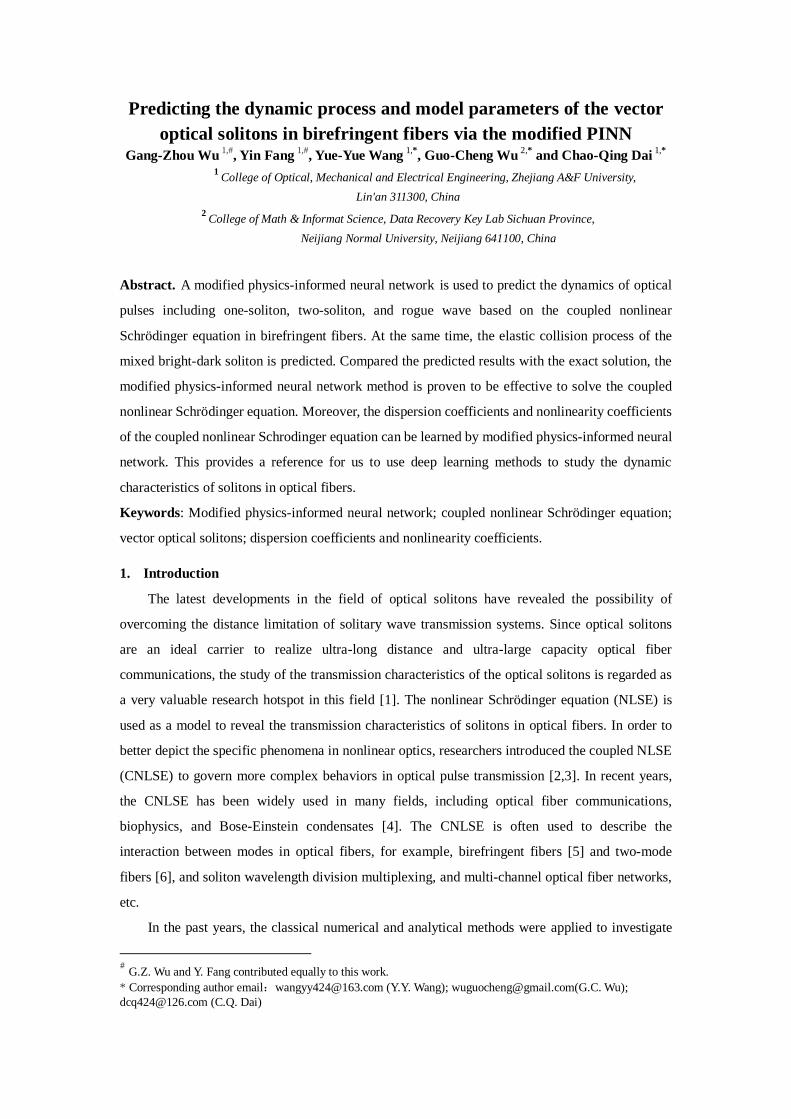
propagates stably in the fiber. In Fig. 2(b), we compare exact solution with the predicted solution

of the bright-bright one soliton at 1.5, 3.5z z for and 2, 4.75z z for , and

we can see that they are completely coincident. The density diagram of error ˆ ( , ) ( , )k k kEr Q t x Q t x

between the exact solution ( , ) ( 1,2)kQ t x k and the predicted solution ˆ ( , )kQ t x is shown in Fig.

2(c), where the large magnitude indicates the larger error. Fig. 2 (d) shows the curve of the loss

function with the number of iterations. The loss function converges to 52.478 10 after 8000

iterations. From the comparison of several aspects in Fig. 2, the prediction result is excellent and

achieves our expectation.

Fig.2. Bright-bright one soliton solutions 1( , )Q z t and 2 ( , )Q z t :(a) The predicted propagation process;

(b) Comparisons between the exact (the blue solid line) and predicted results (the red circle) at

different propagation distances; (c) The density diagram for the error between exact and predicted

results; (d) Curve of the loss function v.s. the iterations.

Next, we discuss which adaptive activation function is an appropriate one when solving one

soliton of the Manakov-type CNLSE. When the structure of the network remains unchanged and

the number of learning is 6000, we study the influence of several conventional activation

functions including sin, cos, tanh, swich functions on the convergence error and convergence

speed of loss function. From Fig. 3, we find that the convergence of sin and switch functions is

similar, the sin function is the best in the convergence rate, however the convergence effect of cos

function is the worst.

1( , )Q z t 2 ( , )Q z t

Fig.3. Convergence curves of loss function for different activation functions when solving one

soliton of the Manakov-type CNLSE.

Table.1. Comparison on prediction of the one soliton solution for the Manakov-type CNLSE by

using different activation functions.

Different

parameters

Activation

functions

time 1r 1m 1Q 2r 2m 2Q loss

cos 7507.69s 63.43% 38.66% 14.9% 5.42% 3.81% 2.87% 0.00205

sin 6663.59s 15.47% 13.46% 3.25% 3.72% 2.53% 0.946% 0.00041

swich 13320.4s 23.10% 19.03% 4.84% 3.90% 2.49% 1.26% 0.00042

tanh 6617.60s 22.24% 18.28% 4.66% 3.65% 2.58% 1.03% 0.00085

In Table 1, these percentages mean relative errors ˆ(| | / ) 100%N N N with the predicted

value N̂ and exact value N , where N includes 1 2 1 2 1, , , ,| |r r m m Q and 2| |Q . From Table 1, we find

that sin, tanh and swich functions have little difference on the error of solution, cos function has

the largest error, yet swich and sin functions have the best performance on the convergence of loss.

However, due to the complexity of swich activation function, it needs longer time to find the

derivative in back propagation. Therefore, we use the improved PINN with using sin function as

the activation function in the following discussion.

3.1.2. Bright-bright two soliton molecule solution

The exact bright-bright two soliton molecule solution is as follows [30]

1.1025 1.05 0.5 3.1 0.5 1.1025 3.05 1.5 0.5

1 2 1 4.1 2 2.1 1 2.05 0.1025 1 2.05 0.1025 1

1.1025 1.05 0.5

2

0.0053 0.0052 2,

1 1.25 0.000034 0.4535 0.7139 0.7139

0.0059

it z it z it z it z

z z z z it z it

it z it

e e e eQ

e e e e e

e eQ

3.1 0.5 1.1025 3.05 1.5 0.5

2 1 4.1 2 2.1 1 2.05 0.1025 1 2.05 0.1025 1

0.0126,

1 1.25 0.000034 0.4535 0.7139 0.7139

z it z it z

z z z z it z it

e e

e e e e e

(9)

with the space-time region [0,2], [ 15,15]z t .

Similarly to the prediction of bright-bright one soliton solution, the prediction result of

bright-bright two-soliton molecule solution is also excellent and achieves the desired effects. In

Fig. 4(a), the predicted bright-bright two soliton molecules maintain a stable propagation at a

certain distance. The two solitons achieve the velocity resonance to form a bound state and keep

an equal distance parallelly transmit without any interaction, and their amplitudes remain

unchanged. In Fig. 4(b), we compare exact solution with the predicted solution of the bright-bright

two soliton molecules at for and for , and their

shapes and structures fit very well. From the density pattern of error between exact solution and

the predicted solution in Fig. 4(c), the error increases along the transmission distance. Fig. 4(d)

shows the curve of the loss function of Eq. (9) and Eq. (10) with the increase of the iterations. The

loss function converges to 56.437 10 and 41.533 10 after 12000 iterations, respectively.

Fig.4. Bright-bright two soliton molecule solutions 1( , )Q z t and 2 ( , )Q z t : (a) The predicted

propagation process; (b) Comparisons between the exact (the blue solid line) and predicted results

(the red circle) at different propagation distances; (c) The density pattern for the error between

exact and predicted results; (d) Curve of the loss function v.s. the iterations.

Next, changing the coefficients of z and t , the exact bright-bright two soliton molecule

solution is as follows

1.44 1.2 1 1.69 3.7 3 1.44 3.8 3 1.69 1.3 1

1 2.4 2 5 4 2.6 2 2.5 0.15 2 2.5 0.15 2

1.44 1.2 1 1.44 3.8 3

2

2 0.0051 0.0052,

1 0.86 0.000042 0.2959 0.48 0.48

0.0066 0.0147

it z it z it z it z

z z z z it z it

it z it z

e e e eQ

e e e e e

e eQ

1.69 3.7 3 1.69 1.3 1

2.4 2 5 4 2.6 2 2.5 0.15 2 2.5 0.15 2,

1 0.86 0.000042 0.2959 0.48 0.48

it z it z

z z z z it z it

e e

e e e e e

(10)

with the space-time region .

0.8, 1.9z z 1( , )Q z t 0.6, 1.4z z 2 ( , )Q z t

[0,2], [ 15,15]z t

Fig.5. Bright-bright two soliton molecule solutions and : (a) The density pattern for

the error between exact and predicted results; (b) Comparisons between the exact (the blue solid

line) and predicted results (the red circle) at different propagation distances.

In Fig.5, changing the value of soliton parameters (coefficients of z and t in the exponential) to

a new solution as a data set. Fig. 5 (a) shows the density plots of the absolute errors. In Fig. 5 (b),

we compare the exact solution and predicted solution of the bright-bright two soliton molecules at

0.8, 1.9z z for 1( , )Q z t and 0.6, 1.4z z for 2 ( , )Q z t . Compared with Fig. 4, the error

increases, but the law of the increase of the error along the transmission distance does not change.

Therefore, changing the coefficients of z and t in the exponential cannot bring any favourable

impact on the results.

3.1.3. First-order rogue wave

The exact first-order rogue wave solution is as follows [32]

1.441 2 2

1.442 2 2

4 11.520.6 (1 ),

2.88(0.0116 ) 8.2944 1

4 11.520.6 (1 ),

2.88(0.0116 ) 8.2944 1

it

it

itQ e

t z t

itQ e

t z t

(11)

with the space-time region [ 1,1], [ 4,4]z t .

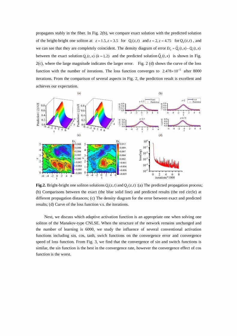
Similarly to the prediction of soliton solution above, the prediction result of first-order rogue

wave is also excellent and achieves the desired effects. In Fig. 6(a), the predicted first-order rogue

wave exhibits high amplitude in the optical fiber. Due to the modulation instability in the optical

fiber, the weak modulation on the plane wave can produce exponential growth along the

transmission distance, and result in rogue waves. In Fig. 6(b), we compare exact solution with the

predicted solution of the first-order rogue wave at for and

for 2 ( , )Q z t , and they have a good match. From the 3D diagram of error between

exact solution and the predicted solution in Fig. 6(c), the error on both sides of the boundary is

relatively large. Fig. 6(d) exhibits the curve of the loss function with the increase of the iterations.

The loss function converges to 31.535 10 after 8000 iterations.

1( , )Q z t 2 ( , )Q z t

0.4, 0.4z z 1( , )Q z t

0.6, 0.8z z

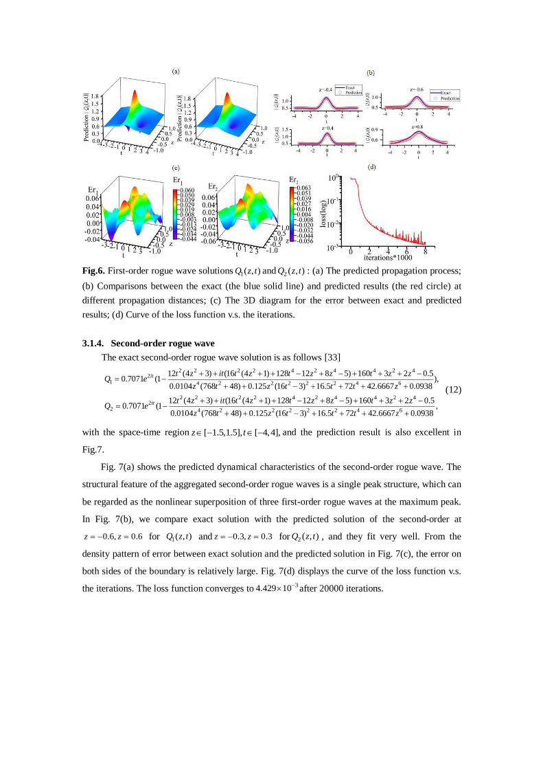
Fig.6. First-order rogue wave solutions 1( , )Q z t and 2 ( , )Q z t : (a) The predicted propagation process;

(b) Comparisons between the exact (the blue solid line) and predicted results (the red circle) at

different propagation distances; (c) The 3D diagram for the error between exact and predicted

results; (d) Curve of the loss function v.s. the iterations.

3.1.4. Second-order rogue wave

The exact second-order rogue wave solution is as follows [33]

2 2 2 2 4 2 4 4 2 42

1 4 2 2 2 2 2 4 6

2 2 2 2 4 22

2

12 (4 3) (16 (4 1) 128 12 8 5) 160 3 2 0.50.7071 (1 ),

0.0104 (768 48) 0.125 (16 3) 16.5 72 42.6667 0.0938

12 (4 3) (16 (4 1) 128 12 80.7071 (1

it

it

t z it t z t z z t z zQ e

z t z t t t z

t z it t z t z zQ e

4 4 2 4

4 2 2 2 2 2 4 6

5) 160 3 2 0.5,

0.0104 (768 48) 0.125 (16 3) 16.5 72 42.6667 0.0938

t z z

z t z t t t z

(12)

with the space-time region [ 1.5,1.5], [ 4,4],z t and the prediction result is also excellent in

Fig.7.

Fig. 7(a) shows the predicted dynamical characteristics of the second-order rogue wave. The

structural feature of the aggregated second-order rogue waves is a single peak structure, which can

be regarded as the nonlinear superposition of three first-order rogue waves at the maximum peak.

In Fig. 7(b), we compare exact solution with the predicted solution of the second-order at

for and for , and they fit very well. From the

density pattern of error between exact solution and the predicted solution in Fig. 7(c), the error on

both sides of the boundary is relatively large. Fig. 7(d) displays the curve of the loss function v.s.

the iterations. The loss function converges to after 20000 iterations.

0.6, 0.6z z 1( , )Q z t 0.3, 0.3z z 2 ( , )Q z t

34.429 10

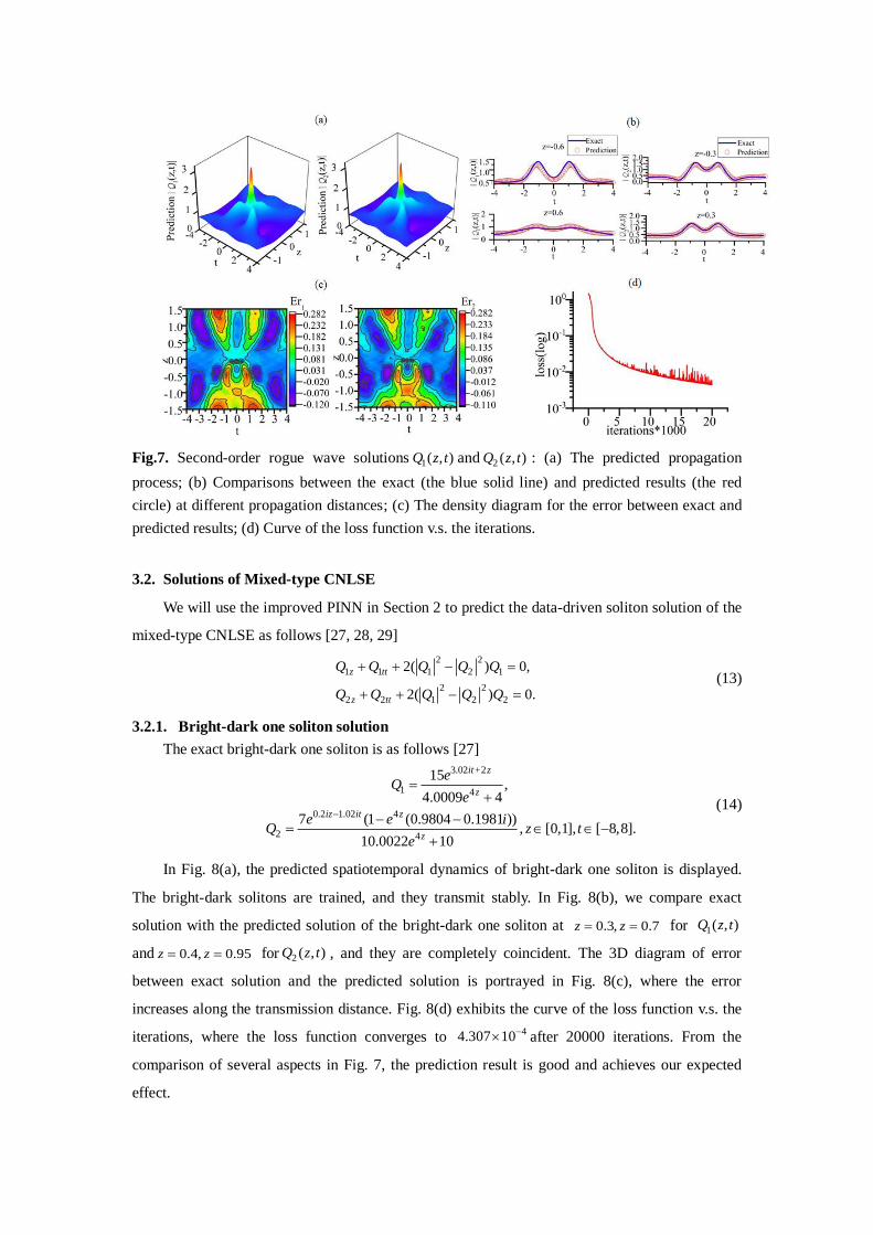
Fig.7. Second-order rogue wave solutions 1( , )Q z t and 2 ( , )Q z t : (a) The predicted propagation

process; (b) Comparisons between the exact (the blue solid line) and predicted results (the red

circle) at different propagation distances; (c) The density diagram for the error between exact and

predicted results; (d) Curve of the loss function v.s. the iterations.

3.2. Solutions of Mixed-type CNLSE

We will use the improved PINN in Section 2 to predict the data-driven soliton solution of the

mixed-type CNLSE as follows [27, 28, 29]

2 2

1 1 1 2 1

2 2

2 2 1 2 2

2( ) 0,

2( ) 0.

z tt

z tt

Q Q Q Q Q

Q Q Q Q Q

(13)

3.2.1. Bright-dark one soliton solution

The exact bright-dark one soliton is as follows [27]

3.02 +2

1 4

0.2 1.02 4

2 4

15 ,

4.0009 4

7 (1 (0.9804 0.1981 )), [0,1], [ 8,8].

10.0022 10

it z

z

iz it z

z

eQ

e

e e iQ z t

e

(14)

In Fig. 8(a), the predicted spatiotemporal dynamics of bright-dark one soliton is displayed.

The bright-dark solitons are trained, and they transmit stably. In Fig. 8(b), we compare exact

solution with the predicted solution of the bright-dark one soliton at 0.3, 0.7z z for

and 0.4, 0.95z z for , and they are completely coincident. The 3D diagram of error

between exact solution and the predicted solution is portrayed in Fig. 8(c), where the error

increases along the transmission distance. Fig. 8(d) exhibits the curve of the loss function v.s. the

iterations, where the loss function converges to after 20000 iterations. From the

comparison of several aspects in Fig. 7, the prediction result is good and achieves our expected

effect.

1( , )Q z t

2 ( , )Q z t

44.307 10

Fig.8. Bright-dark one soliton solutions 1( , )Q z t and 2 ( , )Q z t : (a) The predicted propagation process;

(b) Comparisons between the exact (the blue solid line) and predicted results (the red circle) at

different propagation distances; (c) The 3D diagram for the error between exact and predicted

results; (d) Curve of the loss function v.s. the iterations.

3.2.2. Bright-dark two soliton molecules solution

The exact bright-dark two soliton molecule solution is as follows [27]

0.5 1.4 0.94 1.2 0.94 0.8 0.5

1 0.2 0.44 0.44 0.2 2 2.4 0.4

0.2 0.54 0.

2

(37.1681 1.9318 ) (81.9 5.5941 ) 1.4,

1 (29.345 1.7647 ) (29.345 1.7647 ) 0.6451 0.2089 2246.9

(1

it z it z it z it z

z it it z z z z

iz it

e i e e i eQ

e i e i e e e

e eQ

2 0.44 0.44 0.2 2 2.4 0.4

0.2 0.44 0.44 0.2 2

(24.5387 2.2716 ) (35.0561 0.9754) (0.5954 0.2481 ) (0.1976 0.0678) (2242.218 144.8099 ))

2 (58.6900 3.5294 ) (58.69 3.5294 ) 1.29 0.4178

z it it z z z z

z it it z z

i e e i e e i

e i e i e e

2.4 0.4,

4493.7z ze

(15)

with the space-time region [0,1.6], [ 17.5,17.5],z t and the prediction result of this solution is

also very good in Fig. 9.

Fig. 9(a) shows the predicted dynamic characteristics of bright-dark two soliton molecules.

The propagation velocity of the solitons in the two components is the same, and two solitons form

bound state solitons (also called soliton molecule). The amplitude of two solitons does not change

significantly, and they keep equal interval along the propagation distance. In Fig. 9(b), we

compare exact solution with the predicted solution of the bright-dark one soliton at

for and for , and they get a consistent match.

Fig. 9(c) shows the 3D diagram of error between exact solution and the predicted solution, and the

error increases along the transmission distance. Fig. 9(d) shows the curve of the loss function with

the add of the iterations. The loss function converges to 59.649 10 after 12000 iterations.

0.48, 1.12z z 1( , )Q z t 0.64, 1.44z z 2 ( , )Q z t

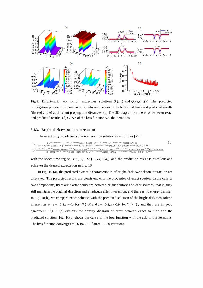
Fig.9. Bright-dark two soliton molecules solutions 1( , )Q z t and 2 ( , )Q z t :(a) The predicted

propagation process; (b) Comparisons between the exact (the blue solid line) and predicted results

(the red circle) at different propagation distances; (c) The 3D diagram for the error between exact

and predicted results; (d) Curve of the loss function v.s. the iterations.

3.2.3. Bright-dark two soliton interaction

The exact bright-dark two soliton interaction solution is as follows [27]

(2.2 1.19 ) (1 1.1 ) (1.4 1.1) (11.8 1.19 ) (1.2 2 ) (4.8 3.54 ) (9.2 3.54 ) (0.8 2 )

1 0.4 14 17 (0.2 3.1 ) (7 2.35 )

1.4 (0.0254 0.3389 ) (0.2561 0.7040 )

1 (0.1890 0.3250 10 ) (0.12

t i z i z t i z i t i t i z i

z t z i t i

e e i e e iQ

e i e

(0.2 3.1 ) (7 2.35 ) 2.4 9.6 2 4.4

0.2 1.02 2.4 9.6 0.4 14 (0.2 3.1 ) (7 2.35 ) (0

2

,63 0.0174 ) (0.1263 0.0174 ) 0.1939 0.5991

7 (1 (0.0746 0.1790 ) (0.15 0.115) (0.0753 0.1504 )

z i t i z t z t

iz it z t z t z i t i z

i e i e e

e e i e e i eQ

.2 3.1 ) (7 2.35 ) 2 4.4

2.4 9.6 0.4 14 17 (0.2 3.1 ) (7 2.35 ) (0.2 3.1 ) (7 2.35 ) 4.4

(0.0183 0.0949) (0.1537 0.5791 ))

10 1.9391 (0.1890 0.3250 10 ) (1.2631 0.1742 ) (1.2631 0.1742 ) 6

z t i z t

z t z t z i t i z i t i t

e i

e e i e i e i e

2,

z

(16)

with the space-time region [ 1,1], [ 15.4,15.4],z t and the prediction result is excellent and

achieves the desired expectation in Fig. 10.

In Fig. 10 (a), the predicted dynamic characteristics of bright-dark two soliton interaction are

displayed. The predicted results are consistent with the properties of exact soution. In the case of

two components, there are elastic collisions between bright solitons and dark solitons, that is, they

still maintain the original direction and amplitude after interaction, and there is no energy transfer.

In Fig. 10(b), we compare exact solution with the predicted solution of the bright-dark two soliton

interaction at 0.4, 0.4z z for and 0.2, 0.9z z for , and they are in good

agreement. Fig. 10(c) exhibits the density diagram of error between exact solution and the

predicted solution. Fig. 10(d) shows the curve of the loss function with the add of the iterations.

The loss function converges to 46.192 10 after 12000 iterations.

1( , )Q z t 2 ( , )Q z t

Fig.10. Bright-dark two soliton interaction solutions 1( , )Q z t and 2 ( , )Q z t : (a) The predicted

propagation process; (b) Comparisons between the exact (the blue solid line) and predicted results

(the red circle) at different propagation distances; (c) The density pattern for the error between

exact and predicted results; (d) Curve of the loss function v.s. the iterations.

4. Parameter prediction of physical model

In this section, we will consider the parameter discovery problem of a data-driven CNLSE

model. The Manakov-type equation is as follows

2 2

1 1 1 2 1 2 1

2 2

2 3 2 4 1 2 2

( ) 0,

( ) 0,

z tt

z tt

iQ Q Q Q Q

iQ Q Q Q Q

(17)

where slowly varying envelopes 1 2,Q Q contain real parts 1 2,r r and imaginary parts 1 2m m , and

variables 1 2 3 4 are the unknown dispersion coefficients and nonlinearity coefficients to be

trained.

The physical models 1,2 ( , )f z t for training are defined as

2 2

1 1 1 1 2 1 2 1

2 2

2 2 3 2 4 1 2 2

: ( ) ,

: ( ) ,

z tt

z tt

f iQ Q Q Q Q

f iQ Q Q Q Q

(18)

which contain real and imaginary parts as 1,2 1,2 1,2( , ) ( , ) ( , )r mf z t f z t if z t ，and we get

2 2 2 2

1 1 1 1 2 1 1 2 2 1

2 2 2 2

1 1 1 1 2 1 1 2 2 1

2 2 2 2

2 2 3 2 4 1 1 2 2 2

2 2 2 2

2 2 3 2 4 1 1 2 2 2

: ( ) ,

: ( ) ,

: ( ) ,

: ( ) .

r z tt

m z tt

r z tt

m z tt

f r m r m r m m

f m r r m r m r

f r m r m r m m

f m r r m r m r

(19)

Our purpose is to minimize the MSE to obtain the approximate value of these unknown

coefficients via the PINN method. The loss function of the neural network is defined as

,rm rm f floss W MSE W MSE (20)

where ,rm fW W are the weights of the initial/boundary and residual terms, and MSE represents the

mean square error

2 2 2 2

1 1 1 1 2 2 2 2

1

2 2 2 2

1 1 2 2

1

1( ( , ) ( , ) ( , ) ( , ) ),

1( ( , ) ( , ) ( , ) ( , ) ).

S

S

N

rm

s

N

f r m r m

s

MSE r z t r m z t m r z t r m z t mN

MSE f z t f z t f z t f z tN

(21)

Using the pseudo spectral method, the one soliton solution of the Manakov-type CNLSE is

discretized into a data set with the space-time region ( , ) [ 6,6] [0,5]z t , and thus the number of

points in the data set is [256 201] . The correct coefficients of the Manakov-type CNLSE are

1 2 3 4 2 . For the sake of the train for unknown dispersion coefficients and

nonlinearity coefficients, we use the 6-layer deep neural network and 50 neurons for each layer

with the number of sampling points 5000sN .. Table 2 shows the training results of these

unknown coefficients and the relative error ˆ=( ) 100% ( =1,2,3,4)eR with the

predicted value ˆ and exact value . From it, we think that the training effect is quite

excellent.

Table.2. Comparison of correct model and identified model obtained by the PINN

Item

CNLSE Model

Relative error eR

1 2 3 4

Correct

equations

2 2

1 1 1 2 1

2 2

2 2 1 2 2

2( ) 0

2( ) 0

z tt

z tt

iQ Q Q Q Q

iQ Q Q Q Q

Identified

equations

2 2

1 1 1 2 1

2 2

2 2 1 2 2

1.000056 2.000033( ) 0

1.000032 2.000016( ) 0

z tt

z tt

iQ Q Q Q Q

iQ Q Q Q Q

0.001657% 0.003195% 0.000799%

Next we will analyze the training effect of the neural network from different perspectives,

such as the category of data sets, the weight of loss function and the anti-interference ability.

We analyze the changes of the unknown coefficients and loss function with the iterations

when we use different solutions such as one soliton, two soliton and rogue wave solutions as data

sets in the inverse problem. Fig. 11(a)-(d) indicates the variation of the unknown coefficients with

the iterations under different data sets. We find that the volatility of the unknown coefficient is the

smallest when a one soliton is used as the data set, and yet this volatility is the largest when the

rogue wave is used as the data set. Fig. 11(e) portrays the change of the loss function for different

data sets with the increase of the number of iterations. It implies that the convergence speed of the

loss function is fastest and the convergence error is smallest when a one soliton is used as the data

set, and yet these performances are the worst when the rogue wave is used as the data set. From

these results, we find that when predicting the physical parameters of the model, the simpler the

structure of the data set, the better the training effect. Therefore, we choose the one soliton

solution as the data set for training the inverse problem.

Fig.11. (a)-(d) the variation of unknown coefficients 1 2 3 4 and (e) the variation of loss

function with the iterations for different data sets.

Fig.12. Variation of unknown coefficients 1 2 3 4 with the iterations for different weights of

the loss function.

In order to find the appropriate component weights of the model and significantly improve

the prediction accuracy, we analyze the changes of unknown parameters with the number of

iterations by changing the weights of the initial/boundary and residual terms of the loss function.

When using the gradient descent method to train the PINN, by adjusting the weight of different

components in the loss function, the gradient values of different components in the loss function

tend to be consistent, which can effectively improve the convergence effect. In Fig. 12, for the

same number of iterations, when : 5 :1rm fW W , the fluctuation of all unknown coefficients is the

smallest and the convergence is faster. Therefore, for this model, : 5 :1rm fW W is the best

choice.

Fig.13. (a) The change of the loss function with the iterations and (b) the change of the error for

the unknown coefficients 1 2 3 4 for different interference noises.

For the sake of the test of the stability for the neural network, we add the interference noise to

the sampling points. Here the 0%-5% noises are added to the sampling points respectively. In Fig.

13(a), with the increase of the noise, the convergence speed of the loss function significantly

slows down, and the convergence error significantly increase. Fig. 13(b) shows the training error

of unknown coefficients for different interference noises. We find that the improved PINN can

accurately predict the unknown coefficients, and the error is still within an acceptable range even

if the sampled data is corrupted by 5% noise. This shows that the neural network we proposed in

Section 2 has a good stability.

5. Conclusion

In conclusion, we propose an improved PINN structure and analyze the activation function,

and thus give a new network structure suitable for the coupled complex function PDEs. Using the

modified PINN method, we predict the soliton transmission process in the frame of the CNLSE,

including bright-bright one soliton, bright-bright two soliton molecules, first-order and

second-order rogue waves, bright-dark one soliton, bright-dark two soliton molecule, and

bright-dark two soliton interactions. To the best of our knowledge, it is the first report to predict

the transmission process of dark solitons by using the improved PINN, and find the dynamic

characteristics of dark solitons predicted by neural network. We find that the errors of

bright-bright one soliton and soliton molecule, bright-dark one soliton and soliton molecule

increase along the transmission distance. The errors at the beginning and end of the first-order and

second-order rogue waves are obviously larger than those in the middle, while the error for the

interaction of bright-dark two soliton has no obvious rule.

For the inverse problem, we mainly conduct research on the model parameter prediction from

two aspects: the data set and the weight of the loss function. For different data sets, it can be seen

that the training effects of neural networks have obvious differences. For the CNLSE, one soliton

solution is an optimal choice to construct the data set. This also conforms to the idea that the

progress of machine learning has been driven by improving the performance of data sets.

Moreover, we find a suitable loss function weight, using which can significantly improve the

convergence speed of the neural network. We have also studied the capacity of resisting

interference for the proposed neural network structure. Our prediction results are still excellent

against high noise interference, which indicates the good stability of our proposed neural network.

Although we have obtained excellent results, there are still issues worthwhile to study. For

such, how to optimize the neural network? How to combine our results with experiments?

Whether this modified PINN method is applicable to other models? These issues will be further

studied in our future works.

References

[1] Agrawal GP. Nonlinear Fiber Optics. Academic Press, New York. 1995.

[2] Nandy S, Barthakur A. Dark-bright soliton interactions in coupled nonautonomous nonlinear

Schrodinger equation with complex potentials. Chaos Solitons & Fractals. 2021;143:110560.

[3] Du Z, Tian B, Qu QX, Chai HP, Zhao XH. Vector breathers for the coupled fourth-order nonlinear

Schrodinger system in a birefringent optical fiber. Chaos Solitons & Fractals. 2020;130:109403.

[4] Bashkin EP, Vagov AV. Instability and stratification of a two-component Bose-Einstein condensate

in a trapped ultracold gas. Physical Review B. 1997;56:6207-12.

[5] Menyuk CR. Stability of solitons in birefringent optical fibers. I: equal propagation amplitudes. Opt

Lett. 1987;12:614-6.

[6] Crosignani B, Porto PD. Soliton propagation in multimode optical fibers. Opt Lett. 1981;6:329-30.

[7] Wu S, Roberts K, Datta S, Du JC, Ji ZC, Si YQ, et al. Deep learning in clinical natural language

processing: a methodical review. Journal of the American Medical Informatics Association.

2020;27:457-70.

[8] Kuutti S, Bowden R, Jin YC, Barber P, Fallah S. A Survey of Deep Learning Applications to

Autonomous Vehicle Control. Ieee Transactions on Intelligent Transportation Systems.

2021;22:712-33.

[9] Surazhevsky IA, Demin VA, Ilyasov AI, Emelyanov AV, Nikiruy KE, Rylkov VV, et al.

Noise-assisted persistence and recovery of memory state in a memristive spiking neuromorphic

network. Chaos Solitons & Fractals. 2021;146:110890.

[10] Marcucci G, Pierangeli D, Conti C. Theory of Neuromorphic Computing by Waves: Machine

Learning by Rogue Waves, Dispersive Shocks, and Solitons. Phys Rev Lett. 2020;125:093901.

[11] Tan T, Peng C, Yuan Z, Xie X, Liu H, Xie Z, et al. Predicting Kerr Soliton Combs in

Microresonators via Deep Neural Networks. Journal of Lightwave Technology. 2020;38:6591-9.

[12] Baumeister T, Brunton SL, Nathan Kutz J. Deep learning and model predictive control for

self-tuning mode-locked lasers. Journal of the Optical Society of America B. 2018;35:617-10.

[13] Lin X, Rivenson Y, Yardimci NT, Veli M, Luo Y, Jarrahi M, et al. All-optical machine learning

using diffractive deep neural networks. Science. 2018;361:1004-8.

[14] Salmela L, Tsipinakis N, Foi A, Billet C, Dudley JM, Genty G. Predicting ultrafast nonlinear

dynamics in fibre optics with a recurrent neural network. Nature Machine Intelligence. 2021;3:344-54.

[15] Narhi M, Salmela L, Toivonen J, Billet C, Dudley JM, Genty G. Machine learning analysis of

extreme events in optical fibre modulation instability. Nat Commun. 2018;9:4923.

[16] Zhang R-F, Bilige S. Bilinear neural network method to obtain the exact analytical solutions of

nonlinear partial differential equations and its application to p-gBKP equation. Nonlinear Dynamics.

2019;95:3041-8.

[17] Bar-Sinai Y, Hoyer S, Hickey J, Brenner MP. Learning data-driven discretizations for partial

differential equations. Proc Natl Acad Sci U S A. 2019;116:15344-9.

[18] Raissi M, Yazdani A, Karniadakis GE. Hidden fluid mechanics: Learning velocity and pressure

fields from flow visualizations. Science. 2020;367:1026-30.

[19] Li J, Chen Y. Solving second-order nonlinear evolution partial differential equations using deep

learning. Communications in Theoretical Physics. 2020;72:105005.

[20] Raissi M, Perdikaris P, Karniadakis GE. Physics-informed neural networks: A deep learning

framework for solving forward and inverse problems involving nonlinear partial differential equations.

Journal of Computational Physics. 2019;378:686-707.

[21] Li J, Chen Y. A deep learning method for solving third-order nonlinear evolution equations.

Communications in Theoretical Physics. 2020;72:115003.

[22] Jun-Cai P, Jun L, Yong C. Soliton, Breather and Rogue Wave Solutions for Solving the Nonlinear

Schrödinger Equation Using a Deep Learning Method with Physical Constraints. arXiv:2011.04949.

[23] Zhou Z, Yan Z. Solving forward and inverse problems of the logarithmic nonlinear Schrödinger

equation with PT-symmetric harmonic potential via deep learning. Physics Letters A.

2021;387:127010.

[24] Wang L, Yan Z. Data-driven rogue waves and parameter discovery in the defocusing nonlinear

Schrödinger equation with a potential using the PINN deep learning. Physics Letters A.

2021;404:127408.

[25] Lu L, Meng X, Mao Z , et al. DeepXDE: A deep learning library for solving differential equations.

arXiv:1907.04502v2.

[26] Dwivedi V, Parashar N, Srinivasan B. Distributed physics informed neural network for

data-efficient solution to partial differential equations. arXiv:1907.08967.

[27] Vijayajayanthi M, Kanna T, Lakshmanan M. Bright-dark solitons and their collisions in mixed

N-coupled nonlinear Schrödinger equations. Physical Review A. 2008;77:013820.

[28] Jiang Y, Tian B, et al. Soliton interactions and complexes for coupled nonlinear Schrödinger

equations. Physical Review E. 2012;85:036605.

[29] Chakraborty S, Nandy S, Barthakur A. Bilinearization of the generalized coupled nonlinear

Schrödinger equation with variable coefficients and gain and dark-bright pair soliton solutions.

Physical Review E. 2015;91:023210.

[30] Radhakrishnan R, Lakshmanan M, Hietarinta J. Inelastic collision and switching of coupled bright

solitons in optical fibers. Physical Review E. 1997;56:2213-6.

[31] Kanna T, Lakshmanan M. Exact soliton solutions of coupled nonlinear Schrodinger equations:

shape-changing collisions, logic gates, and partially coherent solitons. Phys Rev E. 2003;67:046617.

[32] Priya NV, Senthilvelan M, Lakshmanan M. Dark solitons, breathers, and rogue wave solutions of

the coupled generalized nonlinear Schrodinger equations. Phys Rev E. 2014;89:062901.

[33] Zhai BG, Zhang WG, Wang XL, Zhang HQ. Multi-rogue waves and rational solutions of the

coupled nonlinear Schrödinger equations. Nonlinear Analysis: Real World Applications.

2013;14:14-27.