1

Paper 1967-2018

Prediction and Interpretation for Machine Learning Regression Methods D. Richard Cutler, Utah State University

ABSTRACT

The last 30 years has seen extraordinary development of new tools for the prediction of numerical and binary responses. Examples include the LASSO and elastic net for regularization in regression and variable selection, quantile regression for heteroscedastic data, and machine learning predictive method such as classification and regression trees (CART), multivariate adaptive regression splines (MARS), random forests, gradient boosting machines (GBM), and support vector machines (SVM). All these methods are implemented in SAS®, giving the user an amazing toolkit of predictive methods. In fact, the set of available methods is so rich it begs the question, “When should I use one or a subset of these methods instead of the other methods?” In this talk I hope to provide a partial answer to this question through the application of several of these methods in the analysis of several real datasets with numerical and binary response variables.

INTRODUCTION

Over the last 30 years there has been substantial development of regression methodology for regularization of the estimation in the multiple linear regression model and for carrying out non-linear regression of various kinds. Notable contributions in the area of regularization include the LASSO (Tibshirani 1996), the elastic net (Zou and Hastie 2005), and least angle regression (Effron et al. 2002) which is both a regularization method and a series of algorithms that can be used to efficiently compute LASSO and elastic net estimates of regression coefficients. An early paper on non-linear regression via scatter plot smoothing and the alternating conditional expectations (ACE) algorithm is due to Breiman and Friedman (1985). Hastie and Tibshirani (1986) extend this approach to create generalized additive models (GAM). An alternative approach to non-linear regression using binary partitioning are regression trees (Breiman et al. 1984). Multivariate adaptive regression splines (MARS) (Friedman 1991) extended generalized linear and generalized additive models in the direction of modeling interactions, and considerable research of tree methods, notably ensembles of trees, resulted in the development of gradient boosting machines (GBM) (Friedman 2000) and random forests (Breiman 2001). A completely different approach, based on non-linear projections is support vector machines, the modern development of which is usually credited to Vapnik (1995) and Cortes and Vapnik (1995). All of the methods listed above, and more, are implemented in SAS and other statistical packages giving statisticians a very large toolkit for analyzing and understanding data with a continuous (interval valued) response variable. In SAS using the LASSO or fitting a regression tree or random forests is no harder than fitting an ordinary multiple regression with some traditional variable selection. The LASSO has rapidly become a “standard” method for variable selection in regression, and all of these methods lend themselves to larger datasets, where there is a lot of information and statistical significance does not make sense. In this paper I hope to illustrate the use of some of these methods for the analysis of real datasets.

2

GETTING STARTED

In the spirit of the “Getting Started” section of SAS procedure manual entries, we begin with a simple example that illustrates how tree methods can provide insight in situations where linear methods are less effective. The data concern credit card applications to a bank in Australia (Quinlan, 1987). The response variable is coded as “Yes” if the application was approved and “No” if it was not approved. There are 15 predictor variables denoted by A1—A15, some categorical and some numerical. For proprietary reasons the nature of the variables is not available. We note that variables A9 and A10 are code as ‘t’ and ‘f’ which we take to mean ‘true’ and ‘false.’ A total of 666 observations had no missing values and of those 299 persons were approved for credit cards and 367 were not. A first step in a traditional analysis might be to fit a logistic regression, perhaps with some form of variable selection. For this example I used backward elimination with a significance level to stay of 0.05. The code is given below:

proc logistic data=CRX; class A1 A4-A7 A9 A10 A12 A13 / param=glm; model Approved (event='Yes') = A1-A15 / ctable pprob=0.5 selection=b slstay=0.05; roc; run;

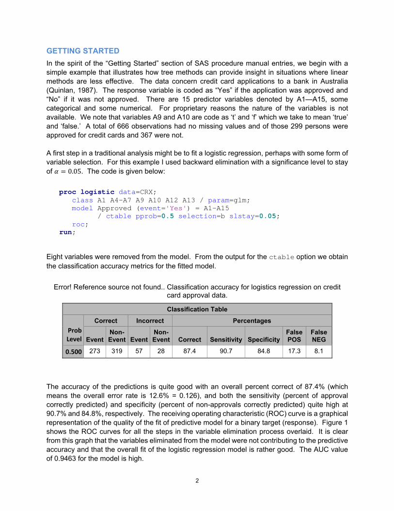
Eight variables were removed from the model. From the output for the ctable option we obtain the classification accuracy metrics for the fitted model.

Error! Reference source not found.. Classification accuracy for logistics regression on credit card approval data.

Classification Table

Prob Level 

Correct Incorrect Percentages

Event Non- Event Event

Non-Event Correct Sensitivity Specificity

False POS

FalseNEG

0.500  273 319 57 28 87.4 90.7 84.8 17.3 8.1

The accuracy of the predictions is quite good with an overall percent correct of 87.4% (which means the overall error rate is 12.6% = 0.126), and both the sensitivity (percent of approval correctly predicted) and specificity (percent of non-approvals correctly predicted) quite high at 90.7% and 84.8%, respectively. The receiving operating characteristic (ROC) curve is a graphical representation of the quality of the fit of predictive model for a binary target (response). Figure 1 shows the ROC curves for all the steps in the variable elimination process overlaid. It is clear from this graph that the variables eliminated from the model were not contributing to the predictive accuracy and that the overall fit of the logistic regression model is rather good. The AUC value of 0.9463 for the model is high.

3

Error! Reference source not found.. ROC Curve for the logistic regression model with variable

selection.

Table 2 contains the estimated coefficients for the variable remaining in the model. From this table it is relatively difficult to tell what variables are most important for determining whether a credit card application will be approved or denied.

0.00

0.25

0.50

0.75

1.00

Sens

itivi

ty

0.00 0.25 0.50 0.75 1.00

1 - Specificity

Model (0.9463)Step 7 (0.9465)Step 6 (0.9470)Step 5 (0.9498)Step 4 (0.9502)Step 3 (0.9504)Step 2 (0.9504)Step 1 (0.9505)Step 0 (0.9506)

ROC Curve (Area)

ROC Curves for All Model Building Steps

4

Error! Reference source not found.. Variable coefficient estimates, standard errors, and P-values.

Analysis of Maximum Likelihood Estimates

Parameter DF EstimateStandard

ErrorWald

Chi-Square Pr > ChiSq

Intercept 1 2.7108 0.8244 10.8132 0.0010

A4 l 1 17.8397 1689.7 0.0001 0.9916

A4 u 1 0.8882 0.3224 7.5884 0.0059

A4 y 0 0 . . .

A6 ? 1 -18.5497 1593.5 0.0001 0.9907

A6 aa 1 -2.8463 0.8545 11.0952 0.0009

A6 c 1 -2.3329 0.8115 8.2632 0.0040

A6 cc 1 -1.2618 0.9473 1.7739 0.1829

A6 d 1 -2.1218 1.0280 4.2604 0.0390

A6 e 1 -1.9622 1.0636 3.4034 0.0651

A6 ff 1 -4.2731 1.0310 17.1793 <.0001

A6 i 1 -3.2242 0.8971 12.9187 0.0003

A6 j 1 -3.2649 1.3861 5.5480 0.0185

A6 k 1 -2.9563 0.8881 11.0813 0.0009

A6 m 1 -2.5419 0.9049 7.8906 0.0050

A6 q 1 -2.1706 0.8490 6.5373 0.0106

A6 r 1 -1.9058 3.8084 0.2504 0.6168

A6 w 1 -1.8939 0.8474 4.9948 0.0254

A6 x 0 0 . . .

A9 f 1 -3.7630 0.3205 137.8444 <.0001

A9 t 0 0 . . .

A11 1 0.1644 0.0463 12.5904 0.0004

A14 1 -0.00220 0.000881 6.2597 0.0124

A15 1 0.000562 0.000182 9.5926 0.0020

An alternative method that one might apply in this situation is a decision tree (Breiman et al. 1984). Decision trees (also known as classification and regression trees) work by recursive partitioning of the data into groups (“nodes”) that are increasingly homogeneous with respect to some kind of a criterion, such as mean squared error for regression trees and either entropy or the Gini index

5

for classification trees. Ultimately the fitted tree is “pruned” back to remove branches and leaves of the tree that are just fitting noise in the data. The pruning process is a critical part of fitting a classification tree: unpruned trees overfit the data and are less accurate predictors for new data. The approach of segmenting the data space is quite different to that of fitting linear, quadratic or additive functions to the predictor variables. In cases where there are strong interactions among predictor variables, classification trees can outperform linear and quasi linear methods. The first step in the fitting of a decision tree is to determine the appropriate size of the fitted tree. A plot of the cross-validated error rate against the size of the fitted tree is obtained using the code below: proc hpsplit data=CRX cvmethod=random(10) seed=123 cvmodelfit plots(only)=cvcc; class Approved A1 A4-A7 A9 A10 A12 A13; model Approved (event='Yes') = A1-A15; grow gini; run;

Error! Reference source not found.. Cross-validated error plotted against the size (number of leaves) of the fitted trees.

6

The plot shows that the minimum cross-validated error rate is achieved by a tree with just 5 leaves, which is a very small tree, and the 1-SE rule of Breiman et al. (1984) selects a tree with just two leaves. That is, the tree splits the data just once. Usually, for large datasets, one would not expect such small trees to be effective predictors but for these data they are, and they provide us with some insight into the data. The tree with just two leaves (terminal nodes branches) splits on the variable A9. Among the persons with a value of ‘t’ on A9, 79.55% were approved for a credit card whereas of the persons with a value of ‘f’ on this variable, only 6.45% were approved for credit cards. One can only speculate as to what this question was, with ‘t’ and ‘f’ being its only possible responses. The overall error rate for this simple split of the data is 13.74%, which is very comparable to the 12.6% for the logistic regression model. How much can the error rate be reduced by using additional variables? The surprising answer is, “not much.” The decision trees with 5 and 10 leaves have error rates of 14.36% and 14.44%, respectively, no better than—and , perhaps, a smidge worse than—the error rate for the simplest decision tree with just two leaves. Even random forests, one of the most accurate machine learning predictive methods, can only reduce the error rate to 12.5%. What this means is that nearly all of the information in these data about the approval or lack of approval of a credit card application is contained in the single variable, A9, and that a very simple decision tee identified this piece of information immediately.

PREDICTION OF WINE QUALITY

The second example of applying machine learning methods for prediction concerns data on the quality of white wine in Portugal (Cortez et al. 2009). The response is the quality of the wine sample on a scale of 0—10, with 10 being the highest quality. The median value of the score of 3 experts was used. Predictor variables are chemical and physical characteristics of the wine samples including pH, density, alcohol content (as a percentage), chlorides, sulfates, total and free sulfur dioxide, citric acid, residual sugar, and volatile acidity. In ordinary multiple linear regression we minimize the residual sum of squares,

⋯

with respect to , , , ⋯ , to obtain the least squares estimates of , , , ⋯ , . The LASSO adds a penalty term to the residuals sum of squares. That is, we minimize

⋯ | |.

7

The parameter is varied and a specific value may be chosen by some criterion, such as AIC or SBC, or to minimize cross-validated prediction error. In the SAS code below, the value of the LASSO parameter is selected by minimizing cross-validated error. Fifty distinct values of are tried. A plot of the coefficients as a function of follows the code. title2 "Regression with LASSO and 10-fold Cross-validation"; proc glmselect data=sasgf.WhiteWine plots=coefficients; model Quality = fixed_acidity volatile_acidity citric_acid residual_sugar chlorides free_sulfur_dioxide total_sulfur_dioxide density pH sulphates alcohol / selection=LASSO(choose=cvex steps=50) cvmethod=split(10); run;

Error! Reference source not found.. Values of regression coefficients for different values of LASSO parameter .

From this plot we see that alcohol is the first variable to have a non-zero coefficient as decreases and volatile_acidity is the second such variable. For this model the cross validated prediction error (CVEX PRESS) is 0.5679 and the final model contains all the predictor variables except citric acid. The LASSO estimates of the regression coefficients are given in Table 3. Increased

8

quality is associated with larger values of alcohol, residual sugar, and pH. Increased quality is associated with smaller values of density, chlorides, and volatile acidity. The coefficient for density is very large relative to the other regression coefficients but that is only a reflection of the fact that the differences in densities among the wines are very, very small. Fixing the random seed for the 10-fold cross-validation ensures that we are able to replicate results exactly when repeating the analysis. Error! Reference source not found.. LASSO estimates of regression coefficients for white wine

data.

Parameter Estimates

Parameter DF Estimate

Intercept 1 121.032634

fixed_acidity 1 0.037306

volatile_acidity 1 -1.873477

residual_sugar 1 0.069450

chlorides 1 -0.357294

free_sulfur_dioxide 1 0.003608

total_sulfur_dioxide 1 -0.000234

density 1 -120.539600

pH 1 0.553261

sulphates 1 0.570229

alcohol 1 0.224899

The second step in the analysis to fit a classification tree to the data. As was the case in the first example, the first step in fitting a classification tree is to determine how large the tree should be. Sample code for doing this is provided below: title2 "Determining Appropriate Size of the Tree"; proc hpsplit data=sasgf.WhiteWine cvmethod=random(10) seed=123 cvmodelfit intervalbins=10000; model Quality = fixed_acidity volatile_acidity citric_acid residual_sugar chlorides free_sulfur_dioxide total_sulfur_dioxide density pH sulphates alcohol; run; By default PROC HPSPLIT “bins” the values of each numerical predictor variable into 100 bins of equal width across the range of the predictor variable. This is a small departure from the original algorithm of Breiman et al. (1984) in which the values of each numerical predictor variable are completely sorted. This modification makes perfect sense for very large datasets for which the cost of complete sorting would be prohibitive. For moderate sample sizes I prefer the original

9

algorithm and by selecting intervalbins=10000 I am effectively making it so there are only 1 or 2 observations per bin, and hence coming close to a full sort of the predictor variables. The plot of cross-validated error against tree size is given below. The cross-validated error is minimized for a large tree that has 57 leaves but the 1-SE rule of Breiman et al. (1984) selects a much smaller tree with only 5 leaves (Figure 5).

Error! Reference source not found.. Cross-validated error against tree size for the white wine data.

In figure 5 we see that at the root node, node 0, there are 4898 observations and the average quality score is 5.8779. The first split is on alcohol, at a value of 10.801. For the 3085 wines with alcohol < 10.801 the average quality score is 5.6055 whereas for the 1813 wines with alcohol ≥ 10.801 the average quality score is 6.3414. Thus the wines with higher alcohol content are rated higher, on average, and this result is consistent with the positive coefficient for alcohol in the regression. The difference between these two values may seem modest but the vast majority of the wines have scores in the range 5—8. For the wines with alcohol < 10.801 the next split is on volatile_acidity at a value of 0.250. The 1475 wines with volatile_acidity < 0.250 have an average quality score of 5.8725 while the 1610 wines with volatile_acidity ≥ 0.250 have an average score of 5.3609. This is consistent with the regression results in which volatile_acidity had a negative coefficient.

10

The second split for the wines with alcohol ≥ 10.801, on free_sulfur_dioxide is much less interesting because only 114 out of the 1813 observations end up in the node corresponding to free_sulfur_dioxide < 11.012. The cross-validated prediction error for the regression tree with 5 leaves is 0.5892, which is slightly larger than the value 0.5679 for the regression using LASSO estimates of the coefficients. By fitting a much larger regression tree, the prediction error may be reduced to 0.5485. Error! Reference source not found.. First two levels of classification tree with 5 leaves (terminal

nodes).

Subtree Starting at Node=0

NodeNAvg

NodeNAvg

alcohol< 10.801

NodeNAvg

volatile_acidity< 0.250

NodeNAvg

volatile_acidity>= 0.250

NodeNAvg

alcohol>= 10.801

NodeNAvg

free_sulfur_dioxide< 11.012

NodeNAvg

free_sulfur_dioxide>= 11.012

11

The third step in the analysis is to apply random forests to determine if higher predictive accuracy might be achieved. Random Forests (Breiman, 2001) takes predictions from many classification or regression trees and combines them to construct more accurate predictions. The basic algorithm is as follows:

1. Many random samples are drawn from the original dataset. Observations in the original dataset that are not in a particular random sample are said to be out-of-bag for that sample.

2. To each random sample a classification or regression tree is fit without any pruning. 3. The fitted tree is used to make predictions for all the observations that are out-of-bag for

the sample the tree is fit to.

4. For a given observations, the predictions from the trees on all of the samples for which the observation was out-of-bag are combined. In regression this is accomplished by averaging the out-of-bag predictions; in classification it is achieved by “voting” the out-of-bag predictions, so the class that is predicted by the largest number of trees for which the observation is out-of-bag is the overall predicted value for that observation.

Many details are omitted from the discussion here, including the number of samples to be drawn from the original data, the size of those samples, whether the samples are drawn with or without replacement, and the number of variables available for the binary partitioning in each tree and at each node. Random Forests may be fit using PROC HPFOREST in SAS® Enterprise Miner™. Here is some sample code for the white wine data: title1 "Fitting Regression Random Forests to White Wine Data"; proc hpforest data=sasgf.WhiteWine maxtrees=200 scoreprole=oob; input fixed_acidity volatile_acidity citric_acid residual_sugar chlorides free_sulfur_dioxide total_sulfur_dioxide density pH sulphates alcohol / level=interval; target Quality / level=interval; run; All the predictor variables are interval valued and go in a single input statement. If there were categorical variables, we would need a second input statement for those variables with the option level=nominal. The response variable, Quality, is also interval-valued and goes into a target statement. The default number of subsets of the data and number of trees to fit is 200. The option scoreprole=oob asks for the out-of-bag error to be reported. One advantage of random forests over other machine learning algorithms is that nearly everything is automated and default settings produce good results in a large number of problems and settings. Table 4 below contains some accuracy results.

Error! Reference source not found.. Random Forests predictive accuracies for selected numbers of trees.

12

Fit Statistics 

Numberof Trees

Numberof Leaves

AverageSquareError

(Train)

AverageSquareError(OOB)

10 10472 0.08523 0.47121

50 51571 0.06476 0.36657

100 102746 0.06214 0.35143

200 205276 0.06076 0.34452

For the full 200 trees the out-of-bag average square error, which is equivalent to the cross-validated prediction error for multiple linear regression and regression trees, is 0.3445, which is quite a bit lower than the value of 0.5679 obtained from the regression using LASSO and the values of 0.5892 and 0.5485 obtained for the regression trees with 5 and 57 leaves, respectively. Thus, this is one situation where the use of a high level machine learning algorithm, such as random forests, gradient boosting machines, or support vector machines, can result in a much higher predictive accuracy than that which traditional regression methods could achieve. A feature of random forests that is very popular with users is its algorithm for determining variable importance. Table 5 contains the variable importances for the white wine data. The data are sorted by the out-of-bag (OOB) mean squared error. The largest value is for alcohol at 0.05605 and there is a substantial drop to density at 0.02292. We decided to refit random forests with just the six most important variables. The out-of-bag error rate was 0.3709, which is a little higher than the value for the random forests fit with all 6 variables, but still much less than for the multiple linear regression model with LASSO estimation and the two regression trees. Error! Reference source not found.. Variable importance from random forests analysis of white

wine data.

Loss Reduction Variable Importance 

Variable Numberof Rules MSE

OOBMSE

Absolute Error

OOB Absolute 

Error

alcohol  24312 0.127562 0.05605 0.082900 0.031738

density  19987 0.096659 0.02292 0.056390 0.005337

volatile_acidity  13769 0.076166 0.01713 0.072654 0.033952

free_sulfur_dioxide  19374 0.080078 0.00786 0.065752 0.016969

chlorides  17315 0.066279 0.00099 0.043994 ‐0.000145

citric_acid  15434 0.053505 ‐0.00788 0.053528 0.011781

residual_sugar  16974 0.053933 ‐0.00982 0.051778 0.008112

fixed_acidity  12515 0.044733 ‐0.01400 0.038773 0.001768

13

Loss Reduction Variable Importance 

Variable Numberof Rules MSE

OOBMSE

Absolute Error

OOB Absolute 

Error

pH  20868 0.056580 ‐0.01843 0.058464 0.006669

total_sulfur_dioxide  19861 0.059472 ‐0.01865 0.059930 0.007552

sulphates  24667 0.055985 ‐0.02316 0.063720 0.007702

What is the nature of the relationship between the individual predictors and the response variable? One approach to answering this is to construct partial dependence plots (Friedman 2000). An alternative is to fit a generalized additive model (Hastie and Tibshirani 1986). For an interval valued response we might assume an approximate normal distribution for the error terms and fit a GAM of the form:

⋯ where the , , ⋯ , are smooth functions of the respective predictor variables.

This model is non-linear in that the may be non-linear functions but it is also additive in the sense that no interactions among predictor variables are included. The primary output from fitting such models is a set of scatter plots of the against the values .

One procedure in SAS for fitting GAMs is PROC GAMPL. Sample code for fitting such a model to the white wine data using only the six most important variables identified by random forests follows: title1 "Fitting a Generalized Additive Model to White Wine Data"; title2 "Using 6 Variables Selected by Random Forests"; proc gampl data=sasgf.WhiteWine plots(unpack)=all; model Quality = s(volatile_acidity) s(citric_acid) s(chlorides) s(free_sulfur_dioxide) s(density) s(alcohol) / dist=normal; run; For the variable alcohol, identified by random forests as the most important variable for predicting quality, we obtain the following plot. This plot is remarkably linear. Error! Reference source not found.. Transformation plot for alcohol in a GAM for the white wine

data.

14

On the other hand, for free_sulfur_dioxide we obtain the following plot, which is noticeably non-linear.

Error! Reference source not found.. Transformation plot for free_sulfur_dioxide in a GAM for the white wine data.

15

For these data most of the transformation plots are approximately linear which raises the question: “If the relationships between most of the predictor variables and the response are (approximately linear), how is it that random forests significantly outperforms a multiple linear regression model for these data?” The answer lies in the fitting of interactions: the multiple linear regression model and even the generalized additive model do not incorporate interactions among predictor variables whereas tree-based methods including random forest and gradient boosting machines do.

CONCLUSION

In this paper we have tried to illustrate the use of machine learning methods for regression problems. In the first example, on credit card applications, a simple decision tree captured the salient information that is available in the data. In the second example, random forests gave significantly more accurate predictions and generalized additive models provided a way to visualize the relationship between predictor variables and the response.

REFERENCES

Breiman, Leo. 2001. “Random forests.” Machine Learning 45(1):5—32.

16

Breiman, Leo and Friedman, Jerome. 1985. “Estimating optimal transformations for multiple regression and correlation.” Journal of the American Statistical Association 80(391):580—598.

Breiman, Leo, Jerome Friedman, Richard Olshen, and Charles Stone. 1984. Classification and Regression Trees. Boca Raton, FL: Chapman & Hall.

Cortes, Corinna and Vladmir Vapnik. 1995. “Support-vector networks.” Machine Learning 20:273—297.

Cortez, Paulo, Antonio Cerdeira, Fernando Almeida, Telmo Matos and Jose Reis. 2009. “Modeling wine preferences by data mining from physicochemical properties.” Decision Support Systems, 47(4):547—553.

Effron, Bradley, Trevor Hastie, Iain Johnstone, and Robert Tibshirani. 2004. “Least angle regression.” Annals of Statistics 32(2):407—499.

Friedman, Jerome. 1991. “Multivariate adaptive regression splines.” Annals of Statistics 19(1):1—67.

Friedman, Jerome. 2001. “Greedy function approximation: The gradient boosting machine.” Annals of Statistics 29(5):1189—1232.

Hastie, Trevor and Robert Tibshirani. 1986. “Generalized additive models.” Statistical Science 1(3):297—310.

Quinlan, J. Ross. 1987. "Simplifying decision trees." International Journal of Man-Machine Studies 27:221—234.

Tibshirani, Robert. 1996. “Regression shrinkage and selection via the LASSO.” JRSS B 58(1):267—288.

Vapnik, Vladmir. 1995. The Nature of Statistical Learning Theory. New York, NY: Springer-Verlag, Inc.

Zou, Hui and Trevor Hastie. 2007. “Regularization and variable selection via the elastic net.” JRSS B 67(2):301—332.

CONTACT INFORMATION

Your comments and questions are valued and encouraged. Contact the author at:

D. Richard Cutler Department of Mathematics and Statistics Utah State University (435) 7975363 Richard.Cutler@usu.edu