prediction markets for economic forecasting · for many prediction market researchers, he will be...
TRANSCRIPT
NBER WORKING PAPER SERIES
PREDICTION MARKETS FOR ECONOMIC FORECASTING
Erik SnowbergJustin WolfersEric Zitzewitz
Working Paper 18222http://www.nber.org/papers/w18222
NATIONAL BUREAU OF ECONOMIC RESEARCH1050 Massachusetts Avenue
Cambridge, MA 02138July 2012
This was prepared for the Handbook of Economic Forecasting, Volume 2. We dedicate this chapterto the memory of John Delaney, founder and CEO of Intrade.com. An innovator and source of inspirationfor many prediction market researchers, he will be sorely missed. The views expressed herein are thoseof the authors and do not necessarily reflect the views of the National Bureau of Economic Research.
NBER working papers are circulated for discussion and comment purposes. They have not been peer-reviewed or been subject to the review by the NBER Board of Directors that accompanies officialNBER publications.
© 2012 by Erik Snowberg, Justin Wolfers, and Eric Zitzewitz. All rights reserved. Short sections oftext, not to exceed two paragraphs, may be quoted without explicit permission provided that full credit,including © notice, is given to the source.

Prediction Markets for Economic ForecastingErik Snowberg, Justin Wolfers, and Eric ZitzewitzNBER Working Paper No. 18222July 2012JEL No. C53,G14
ABSTRACT
Prediction markets--markets used to forecast future events--have been used to accurately forecast theoutcome of political contests, sporting events, and, occasionally, economic outcomes. This chaptersummarizes the latest research on prediction markets in order to further their utilization by economicforecasters. We show that prediction markets have a number of attractive features: they quickly incorporatenew information, are largely efficient, and impervious to manipulation. Moreover, markets generallyexhibit lower statistical errors than professional forecasters and polls. Finally, we show how marketscan be used to both uncover the economic model behind forecasts, as well as test existing economicmodels.
Erik SnowbergDivision of Humanities and Social SciencesMC 228-77California Institute of TechnologyPasadena, CA 91125and [email protected]
Justin WolfersBusiness and Public Policy DepartmentWharton School, University of Pennsylvania3620 Locust WalkRoom 1456 Steinberg-Deitrich HallPhiladelphia, PA 19104-6372and [email protected]
Eric ZitzewitzDepartment of EconomicsDartmouth College6106 Rockefeller HallHanover, NH 03755and [email protected]
1 Introduction
Market prices, in the form of gambling odds, have been used to forecast events since at least
the beginning of the sixteenth century. The use of such prices had a heyday in the early
twentieth century, when gambling odds on elections were printed daily in newspapers such
as The New York Times. This was followed by a decline in popularity, due largely to the
advent of scientific polling (Rhode and Strumpf, 2004, 2008). Scientific interest in market
prices as tools for forecasting was kindled in the second half of the twentieth century by
the efficient markets hypothesis and experimental economics (Plott and Sunder, 1982, 1988;
Berg et al., 2008). This scientific foundation, coupled with advances in telecommunications—
which allowed prices to be shared in real time across companies and the globe—has lead to
resurgent interest in using markets for forecasting (Snowberg, Wolfers and Zitzewitz, 2007b).1
Despite this long history, and markets’ proven track-record of providing accurate forecasts
of uncertain events, prediction markets—markets used to forecast future events—are largely
unused in economic forecasting. There are some exceptions: the difference in yields between
inflation protected and standard government bonds is used to forecast inflation, and futures
contracts are sometimes used to forecast commodity prices, such as the price of oil. However,
as other chapters in this volume reveal, these uses are accompanied by concerns about what
else, other than information about future events, may be lurking in market prices (Alquist
and Vigfusson, 2012; Duffee, 2012; Wright and Faust, 2012; Zhou and Rapach, 2012).
This chapter brings together the latest research on prediction markets to further their
utilization by economic forecasters. We begin by providing a description of standard types
of prediction markets, and an heuristic framework useful in understanding why prediction
markets do, and sometimes do not, make useful predictions. We then show that, in practice,
prediction markets often have a number of attractive features: they quickly incorporate
new information, are largely efficient, and impervious to manipulation. Moreover, markets
1See Wolfers and Zitzewitz (2008a) for an overview, and Tziralis and Tatsiopoulos (2007) for an exhaustiveliterature review.
1

generally outperform professional forecasters and polls. Finally, we argue that examining
co-movement in market prices, through, for example, event studies, can be used to shed light
on the underlying economic model of market participants. We conclude with a short list of
open questions that may be of particular interest to economic forecasters.
2 Types of Prediction Markets
A prediction market is generally implemented as a wager (or contract) that pays off if
a particular outcome, such as an economic indicator taking a particular value y, occurs.
Assuming that both the efficient markets hypothesis holds, and that the market acts as
a risk-neutral representative trader, the price of the contract will be the best estimate of
various parameters tied to the probability of that outcome. While these assumptions are
clearly too stark, in many settings the biases from violations are quite small, and in practice,
the predictions extracted under these assumptions have been shown to be quite reliable.2
Table 1 summarizes three standard types of contracts. These contracts can be used to
elicit the probability of a particular outcome occurring, or, if the outcome takes on numerical
values, the expected mean or median.
Following the nomenclature introduced in Wolfers and Zitzewitz (2004), a “winner-takes-
all” contract costs some amount $p, and pays off, say, $100, if y, initial unemployment claims
(in thousands), are reported to be between y = 330 and y = 340. Under the assumptions
above, the price represents the market’s expectation of the probability that initial unemploy-
ment claims will be in this range. A family of such contracts with payoffs tied to all likely
values of the event can elicit the entire distribution of the market’s beliefs. For example, a
2The literature has considered two possible divergences. When prediction market security outcomes arecorrelated with a priced asset market factor, such as the overall level of the stock market, prices can beabove objective probabilities if a prediction market security offers hedging value. In most applications,differences between risk-neutral and objective probabilities are smaller (see, for example, Snowberg, Wolfersand Zitzewitz, 2007a; Wolfers and Zitzewitz, 2008b). A second issue is that when beliefs differ, a market mayaggregate beliefs in a different way than is statistically optimal. Wolfers and Zitzewitz (2006) find, however,that under most reasonable assumptions about risk-aversion, prices are close to the wealth-weighted meanbelief (see also, Manski, 2006; Gjerstad, 2005; Ottaviani and Sørensen, 2010).
2

Table 1: Contract Types: Estimating Uncertain Quantities or Probabilities
Contract Example DetailsReveals marketexpectation of...
Winner-takes-all Outcome y: Level of Contract costs $p. Probability that outcomeinitial unemployment Pays $1 if and only if y occurs.claims (in thousands). event y occurs. Bid
according to the valueof $p.
Index Contract pays $1 for Contract pays $ y. Mean value ofevery 1,000 initial outcome y: E[y].unemploymentclaims.
Spread Contract pays even Contract costs $1. Median value ofmoney if initial Pays $2 if y > y∗. outcome y.unemployment Pays $0 otherwise.claims are greater Bid according to thethan y∗. the value of y∗
Notes: Adapted from Table 1 in Wolfers and Zitzewitz (2004).
set of contracts, one of which pays off if initial unemployment claims are between 310 and
320, another that pays off if they are between 320 and 330, and so on, recovers the markets’
p.d.f. (integrated over bins of 10,000) of initial unemployment claims.3
However, if a researcher is interested in simply obtaining moments of the market’s distri-
bution, an “index” contract may be more useful. Such a contract has an unknown payoff tied
to the value of the outcome. Continuing the example from above, if y is initial unemployment
claims (in thousands), the price for this contract represents the market’s expectation of the
outcome: E[y]. Higher order moments can be elicited by using multiple index contracts. For
example, by adding a contract that pays off the square of initial unemployment claims y2,
one can recover the variance of the market’s beliefs: E[y2] − E[y]2.
Finally, a “spread” contract allows a researcher to elicit a robust measure of the central
3The techniques contained in Bakshi and Madan (2000) and Carr and Madan (2001) may be especiallyuseful in analyzing such a family of contracts.
3

tendency of the market’s beliefs. These contracts, which are familiar to bettors on basketball
and American football, feature a fixed cost and fixed payoff if an indicator is below the spread
value, however, the spread’s value y∗ changes as contracts are bought and sold. That is, if
the payoff is twice the cost, say $2 and $1, respectively, the value of the spread y∗ is allowed
to vary until an equal number of contracts are bought and sold. The value of the spread
y∗ is thus the median of the market’s distribution. By varying the cost and payoff of the
contract, it is possible to elicit other percentiles. For example, a contract that costs $4 and
pays $5 when y > y∗ elicits the value y∗ such that the market believes Prob(y < y∗) = 0.8.
We should note that although all of the contracts discussed above have been utilized
to some extent, winner-take-all contracts on a single event are by far the most popular
form of prediction markets. This is largely because such contracts are straight-forward for
market participants to understand. More research is needed to understand the benefits, and
limitations, of other forms of contracts and families of those contracts.
2.1 Formats for Administering Prediction Markets
Most prediction markets, like those available on the industry standard Intrade.com, are
implemented like equity markets. That is, buyers and sellers interact through a continuous
double auction. However, a number of other designs have been suggested, and, in some cases
gained traction. The major variations are play-money markets, pari-mutuel markets, and
market scoring rules.
Due to concerns about speculation and manipulation, the U.S. Commodities Futures
Trading Commission has tightly regulated prediction markets (Arrow et al., 2008). Thus,
many markets, especially internal corporate markets, have been established using play money
(Bell, 2009). For example, Lumenlogic, a leading provider of prediction markets to busi-
nesses, and the Hollywood Stock Exchange, which seeks to forecast entertainment related
outcomes, have chosen to run their exchanges using a virtual currency that can either be
traded in for prizes, or amassed for prestige. Existing research suggests that these virtual
4

currency prediction markets can be as accurate as real-money markets, but more research is
needed (Servan-Schreiber et al., 2004).
Economic Derivatives, large scale markets run by Goldman Sachs and Deutsche Bank
that were tied directly to macroeconomic outcomes, such as initial unemployment claims
and non-farm payrolls, were run as occasional, pari-mutuel markets. This structure, familiar
from gambling on horse races, allows traders to buy or sell contracts on specific ranges of the
economic indicator—similar to the example index contract above. However, the price is not
determined until the auction closes—although estimated prices are displayed based on the
price that would prevail if no more orders were posted. Once the market is closed and the
outcome is realized, pari-mutuel markets split the total amount wagered among those who
wagered on the correct range. If, for example, the actual initial unemployment claims (in
thousands) were between y = 330 and y = 340, then each contract on that range would split
the total amount wagered on all ranges.4 Like the example of index contracts given above, a
pari-mutuel market structure will recover the full p.d.f. of the market’s beliefs. However, the
pari-mutuel market does this with a single market, rather than the numerous index contracts
that would need to be set up.5
Finally, market scoring rules (Hanson, 2003, 2007) have shown great promise in the
lab, and have been used by Microsoft and other corporations for their internal markets
(Abramowicz, 2007). This format starts with a simple scoring rule—which rewards a single
person for the accuracy of his or her prediction—and allows other entrants to essentially
purchase the right to the reward when they believe they have a more accurate prediction.
This format is used largely to reduce speculation and deal with problems that typically
arise from thin markets. However, like standard scoring rules, market scoring rules require
a market maker to subsidize the reward for accurate predictions. Still, in some situations,
4The Economic Derivatives market used a more sophisticated algorithm to determine prices in such away to maximize trades. For a more detailed description of the design of these markets see Gurkaynak andWolfers (2005).
5Plott (2000) gives an example using a similar structure inside of a large business to produce a fullp.d.f. sales forecast.
5

this may be a small price to pay for the added benefits.
3 Why Prediction Markets Work
Three inter-related facets lead to prediction markets’ ability to produce accurate, reliable
forecasts. First, the market mechanism is essentially an algorithm for aggregating informa-
tion. Second, as superior information will produce monetary rewards, there is a financial
incentive for truthful revelation. Third, and finally, the existence of a market provides longer-
term incentives for specialization in discovering novel information and trading on it. While
these facets are inherent in any market, other forecasting mechanisms, such as polling, or
employing professional forecasters, lacks one or more of them. For example, polling lacks
incentives for truthful revelation, and professional forecasters may have other motivations
than simply forecast accuracy (Ottaviani and Sørenson, 2012).
This section documents several examples of how these facets lead to desirable character-
istics in practice, such as the rapid incorporation of information, a lack of arbitrage oppor-
tunities, and a resistance to manipulation. We then turn to a brief overview of design flaws
that may lead markets to fail, and conclude this section with a discussion of more speculative
uses of prediction markets. The next section compares prediction market accuracy to other
available methods.
As an illustration of the speed at which prediction markets incorporate new information,
consider the killing of Osama bin Laden. At 10:25 p.m. Eastern time on May 1st, 2011,
Keith Urbahn, the former chief of staff to Defense Secretary Donald Rumsfeld used the
social media service Twitter to announce, “So I’m told by a reputable person they have
killed Osama Bin Laden. Hot Damn.” The first panel of Figure 1 shows the reaction of
a prediction market tracking the probability that Osama bin Laden would be captured or
killed by December 31st, 2011. Within moments of Urbahn’s statement, the price of this
contract, which generally saw very little trading, started to rise. Within 25 minutes of this
6

Figure 1: Information is incorporated quickly, and continuously across time.
0
2
4
6
Av
erag
e A
bso
lute
Fo
reca
st E
rro
r(V
ote
Sh
are
%)
0306090120150Days Until Election
Notes: Second panel based on data from the IEM, 1988–2000, available at <http://www.biz.uiowa.edu/iem>.Adapted from Wolfers and Zitzewitz (2004).
7

Figure 2: Prediction markets show little evidence of arbitrage opportunities.
$30
$40
$50
$60
$70
$80
Bid
an
d A
sk P
rice
sC
on
trac
t p
ays
$1
00
if
Sch
war
zen
egg
er W
ins
16 Sep 03 23 Sep 03 30 Sep 03 07 Oct 03
Intrade
World Sports Exchange
Notes: Data underlying lower line for each data source are bids, data underlying upper line for each datasource are asks. Prices collected electronically every four hours by David Pennock, adapted from Wolfersand Zitzewitz (2004).
initial announcement, the probability implied by this contract had risen from 7% to nearly
99%. This final estimate was eight minutes before any mainstream media outlet “broke the
story” of bin Laden’s death.
Moreover, prediction markets continuously incorporate new information. The second
panel of Figure 1 shows the accuracy of election forecasts from the Iowa Electronic Markets
(IEM), an academic-run prediction market based at the University of Iowa, across time. The
figure shows quite clearly that as the election approaches, and more information is revealed
about likely outcomes, the forecast error decreases steadily.6
Prediction markets also evince little evidence of arbitrage opportunities. Contracts within
a single exchange are generally arbitrage linked. For example, a rapid increase in the price
of a contract tied to the victory of a particular political candidate is generally accompanied
6Additionally, the error is generally smaller than polls across time, see Figures 6 and 7, and the surround-ing discussion.
8
by decreases in the prices of contracts linked to other candidates, so the implied prob-
ability of someone winning an election stays quite close to 100%. Although the general
winnowing of prediction market companies in the 2000s makes it more difficult to compare
prices across exchanges, Figure 2 shows that in 2003 the prices of different contracts tied to
Arnold Schwarzenegger becoming the governor of California exhibited significant variation,
but moved in lockstep.7
Additionally, prediction markets are quite difficult to manipulate. Attempts by party
bosses to manipulate the price of their candidates in turn of the century gambling markets
were largely unsuccessful, as were more recent attempts by candidates themselves (Rhode
and Strumpf, 2008; Wolfers and Leigh, 2002). More recent, and systematic, attempts at
manipulation yielded only brief transitory effects on prices. Rhode and Strumpf (2008)
placed random $500 bets (the largest allowed) on the IEM and found that prices quickly
returned to pre-manipulation levels. Camerer (1998) placed large bets in pari-mutuel horse
racing markets (which he cancelled moments before the race) to see if this would create
a bandwagon effect of follow-on bets. It did not. Finally, evidence from experimental
prediction markets, run in the lab, show similar results. In a first experiment where some
participants were incentivized to try to manipulate prices, there was little evidence that these
participants were successful (Hanson, Oprea and Porter, 2006). A second experiment based
incentives on whether or not observers of the market price could be manipulated. Similarly,
there was little evidence that manipulators affected the beliefs of observers (Hanson et al.,
2011). Indeed, manipulators may increase the accuracy of prediction markets by providing
more liquidity (Hanson and Oprea, 2009).
Anecdotal reports of attempts at manipulation abound, and reports indicate they have
generally been unsuccessful. One exception we are aware of is manipulation of a contract tied
7There was an arbitrage opportunity in 7 of the 105 time periods for which we have data, and the averagesize the arbitrage opportunity was 1.17 points. However, as positions cannot be moved across exchanges,executing on that opportunity would require holding a long position on one exchange, and a short positionon the other until expiry. That is, one must hold $200 in positions for the duration of the contract in ordergain $1 in arbitrage.
9

to Hillary Clinton’s probability of winning the presidency in 2008, conditional on winning
the Democratic nomination. A single, large trader bought contracts on Intrade.com at prices
that implied Clinton was much more electable by the general electorate than her Democratic
competitors. While the manipulator was able to keep prices high for a significant period of
time, the profit opportunity was noticed and discussed by other traders, resulting in huge
losses for the large trader. Moreover, the manipulated price garnered only one mention in
the mainstream media.8
Finally, in most cases, prediction markets seem to satisfy at least the weak form of
the efficient markets hypothesis. That is, there is no evidence that trading on past prices
can result in a profit. This has been explicitly demonstrated for prediction markets by
Leigh, Wolfers and Zitzewitz (2003), Tetlock (2004), and Berg, Forrest and Rietz (2006).
In particular, Leigh, Wolfers and Zitzewitz (2003) test prediction markets related to the
demise of Sadaam Hussein, and find that an augmented Dickey-Fuller test cannot reject the
null that those markets follow a random walk. They also find that a KPSS test rejects the
null that prices are trend-stationary. Berg, Forrest and Rietz (2006) also finds that prices
in the Iowa Electronic Markets follow a random walk. Finally, Tetlock (2004) finds some
evidence of mispricing in prediction markets concerning sporting events, including evidence
of over-reaction to news. However, the mispricing is not large enough to allow for profitable
trading strategies. Moreover, Tetlock (2004) finds no evidence of mispricing in prediction
markets about financial events on the same exchange. More evidence about the efficiency of
prediction markets can be found in the large literature on gambling markets. This literature
generally finds that betting markets are weakly efficient (discussed in several chapters of
Vaughn Williams, 2005; Hausch and Ziemba, 2007).
3.1 Why They (Sometimes) Fail
8A summary of this (successful) attempt at manipulation attempt can be found in Zitzewitz (May 30,2007).
10

Although prediction markets generally function quite well, design flaws sometimes prevent
reliable forecasts. These flaws generally lead to a lack of noise traders (or thin markets)
that reduces incentives for discovering, and trading on the basis of, private information
(Snowberg, Wolfers and Zitzewitz, 2005). In order to attract noise traders, the subject of a
prediction market must be interesting and information must be widely dispersed.
Prediction market contracts must be well specified, so that it is clear when they will
(and will not) pay off. However, this specificity may be in tension with making a contract
interesting for traders. For example, in 2003, InTrade ran markets that asked, “Will there
be a UN Resolution on Iraq (beyond #1441)?” and “Will Saddam be out of office by June
30?” The former is clearly better specified, but the latter had much higher trading volume.
Moreover, even the former has some ambiguity: what does it mean for a UN Resolution to
be “on” Iraq?
Noise traders may quite rationally choose not to trade in markets where there is a high
degree of insider information. For example, despite the high intrinsic interest in who a
Supreme Court nominee will be, markets on this topic have routinely failed. This may be
due to the fact that most traders are aware that there are very few people with actual
information on who the President’s choice will be. This anecdote underlines the importance
of prohibiting insider trading: for instance, a market to predict the Institute for Supply
Management’s (ISM’s) business confidence measure would be unlikely to function if it were
well known that ISM employees were trading in it.
An extreme form of information not being widely dispersed is when there is no information
at all to aggregate. For example, prediction markets on whether weapons of mass destruction
(WMDs) would be found in Iraq predicted they would very likely be found. The false
confidence that could be inspired by such an estimate ignores the fact that there was no
information being aggregated by these markets. That is to say, it was unlikely that anyone in
Iraq, who might actually have some information (perhaps based on rumors, past experience,
or informal discussions with friends and relatives in the government) about whether Iraq’s
11

Figure 3: The favorite-longshot bias is the most prominent pricing anomaly in sports betting.
Even Break
−20
−40
−60
−80
Rat
e o
f R
etu
rn p
er D
oll
ar B
et (
%)
1/3 1/2 Evens 2/1 5/1 10/1 20/1 50/1 100/1 200/1Odds (Log Scale)
US: 1992−2001
Australia: 1991−2004
UK: 1994−2004
Griffith, Am. J. Psych 1949
Weitzman, JPE 1965
Harville, JASA 1973
Ali, JPE 1977
Jullien and Salanie, JPE 2000
Data Source
Notes: Adapted from Snowberg and Wolfers (2010).
WMD program was likely to exist or not, was trading in these markets.
Finally, it is unclear to what extent prices in prediction markets may be affected by
behavioral biases. The most prominent, and well-understood, pricing anomaly in sports
betting is the favorite-longshot bias. This pattern, shown across many studies and countries
by Figure 3, comes from long-shots being overbet and favorites being underbet relative
to their risk-neutral probabilities of victory.9 Thus, interpreting the prices of gambles on
horses as probabilities will tend to underestimate a horse’s probability of victory when that
probability is very high, and tend to overestimate a horse’s probability of victory when that
probability is very low.
A similar pattern is documented in 2004 U.S. election markets from InTrade.com in
Figure 4. Almost all of the contracts that traded above a price of 50 won, and almost all of
9As the favorite-longshot bias is a divergence between risk-neutral implied probabilities and actual proba-bilities, it is also related to pricing phenomena in options markets, see Rubinstein (1994); Tompkins, Ziembaand Hodges (2008).
12

those that traded below a price of 50 lost, implying that those markets which predicted a
high probability of one candidate winning underpredicted the actual probability of victory,
while those that predicted a low probability of victory overpredicted the actual probability.
Recent work has attributed the favorite-longshot bias in gambling markets to behav-
ioral phenomena, with Jullien and Salanie (2000) attributing it to asymmetries in the way
traders value gains and losses, and Snowberg and Wolfers (2010) attributing it to mispercep-
tions of probabilities. Regardless of the underlying explanation, a good rule of thumb is to
use extreme caution when interpreting results based on contracts that imply a risk-neutral
probability between 0 and 10%, or 90% and 100%.
Figure 4: The favorite-longshot bias is also apparent in prediction markets.
0%
6%
94%
100%
0
25%
50%
75%
100%
% o
f C
and
idat
es w
ho
Wo
n
0−25% 26−50% 51−75% 76−100%
Implied Probability−−Night before 2004 U.S. Election
Notes: Data pools 50 markets on the state-by-state outcome of the electoral college, and 34 markets onU.S. Senate races on Intrade.com (then: Tradesports.com).
3.2 Bleeding Edge Design
The stories of failure above lead to some straight-forward rules for designing prediction
markets: make sure the question is well-defined, that there is dispersed information about
13
the question, and that there is sufficient interest in the question to ensure liquidity. However,
such simple guidelines leave much to be desired. For example, what if the question is
inherently difficult to define, or there simply is not sufficient interest in the question? These
problems have been confronted by corporations using prediction markets, and although there
is little academic work on their experiences, we do our best to summarize those experiences
here.10
Corporations are attracted to prediction markets as they can potentially pass unbiased
information from a company’s front-line employees to senior management.11 However, many
questions of interest to executives are not widely interesting, nor are there many employees
that have relevant information. This creates a lack of liquidity in markets, perhaps leading
to no trading, or, worse, inaccurate predictions. Microsoft has responded to this problem by
using a market-making algorithm, which is a variation of the market scoring rules described
above (Berg and Proebsting, 2009). The market maker’s function in a prediction market is
similar to that in any other equity market: it buys and sells when other market participants
are not available. However, unlike most market-makers, market-making algorithms are less
concerned with making money, and often prefer to lose money if it is likely to increase
informational efficiency.
Separately, Hewlett-Packard has used a structure similar to a pari-mutuel market in which
a small number of participants are forced to take bets. This implementation is particularly
interesting as the market designers use other information about the market participants,
such as their risk-attitudes and social connections, to enhance the market’s efficiency. For
example, if three participants who are known to be friends all bet heavily on the same
potential outcome, the market interprets these bets as being based on redundant information,
10Firms whose internal prediction markets have been mentioned in the public domain include AbbottLabs, Arcelor Mittal, Best Buy, Chrysler, Corning, Electronic Arts, Eli Lilly, Frito Lay, General Electric,Hewlett-Packard, Intel, InterContinental Hotels, Masterfoods, Microsoft, Motorola, Nokia, Pfizer, Qual-comm, Siemens, and TNT (Cowgill, Wolfers and Zitzewitz, 2009). The results of these markets are rarelyreported, as they often entail sensitive information.
11Side benefits, such as creating a sense of empowerment and fun among a company’s front line employeeshave also been reported, see Strumpf (2009).
14

and lowers the impact of each bet on the overall price (Chen and Krakovsky, 2010).
One of the most prominent corporate applications of prediction markets has been to
manage R&D portfolios. This is done through “idea markets” which allow employees to buy
stock in particular ideas in order to determine which idea(s) are likely to be most profitable
for the company. However, the price of the contract depends only on supply and demand,
and is not tied to any actual outcome (such as profit if the product is eventually launched).
These markets are sometimes described as “preference markets”, and they are similar to
pure beauty contests (Marinovic, Ottaviani and Sørenson, 2011). Thus, there is the risk of
divergence between the question of interest, and what the market can answer. Indeed, GE,
one of the most prominent users of idea markets has found that the originators of ideas trade
aggressively to raise the price of their idea and lower the price of other’s ideas (Spears et al.,
2009).
Despite the theoretical problems associated with such markets, and the lack of a clear
way to evaluate their performance, they are increasingly popular. This has driven a range of
experiments with different designs. These experiments vary many of the fine details of market
structure, and hence are not easily summarized. Details can be found in Lavoie (2009), Spears
et al. (2009), Dahan, Soukhoroukova and Spann (2010). An unusually detailed description
of the design and evaluation of a prediction market to help with technology assessment can
be found in (Gaspoz, 2011).
A final design constraint is the uncertain legal and regulatory environment surrounding
prediction markets (Arrow et al., 2008). The current legal situation is summarized in Bell
(2009). Companies are likely best served by consulting with a professional purveyor of
prediction market services, a list of which can be found in Berg and Proebsting (2009).
4 Forecast Accuracy
15

The most notable feature of prediction markets is the accuracy of the forecasts they produce.
We illustrate this accuracy through a number of case studies, beginning with an examination
of the sole, large-scale, prediction market run on macro-economic outcomes, the Economic
Derivatives markets mentioned earlier. We supplement this with case studies from businesses
and politics, where prediction markets have been more extensively studied, and arguably,
have had a much larger impact.
4.1 Macro Derivatives
For a few years, beginning in October 2002, Goldman Sachs and Deutsche Bank operated
markets tied directly to macro-economic outcomes.12 These markets, described as “Economic
Derivatives”, allowed investors to purchase options with payoffs that depended on: growth
in non-farm payrolls, retail sales, levels of the Institute for Supply Management’s (ISM’s)
manufacturing diffusion index (a measure of business confidence) and initial unemployment
claims, among others. The payoffs in these markets were tied to particular data releases,
and thus allowed investors to hedge against specific, event-based, risk. The performance of
these markets was analyzed by Gurkaynak and Wolfers (2005); this subsection summarizes
their main results.
The forecasts gleaned from these markets can be compared with a survey based forecast
released by Money Market Services, which typically averages predictions across approxi-
mately 30 forecasters, as in Figure 5.13 Visual inspection shows that the market-based
forecast are weakly more accurate than the survey-based forecast, and this is verified by a
numerical analysis.
Table 2 examines both the mean absolute error and mean squared error of both forecasts,
normalized by the average forecast error from past surveys. The normalization makes the
data across all four series sufficiently comparable to pool all data in the fifth column. For
12These markets no longer exist, presumably because the trading volume was not sufficiently high as tomake them profitable.
13Money Market Services was acquired by Informa in 2003, so some of the survey-based data comes fromAction Economics and Bloomberg.
16

Figure 5: Macro derivatives are weakly more accurate than survey forecasts.
−400
−200
0
200
400
−400 −200 0 200 400
Non−Farm Payrolls
45
50
55
60
65
45 50 55 60 65
Business Confidence (ISM)
−1
−.5
0
.5
1
1.5
−1 −.5 0 .5 1 1.5
Retail Sales (excluding Autos)
300
320
340
360
380
300 320 340 360 380
Initial Unemployment Claims
Rel
ease
d V
alue
(Act
ual
)
Forecast Value
Economic Derivatives Mean Forecast Survey: Average Across Forecasters
Notes: Adapted from Gurkaynak and Wolfers (2005).
all four series, the market-based forecast is more accurate than the survey-based forecast.
Across all series, relying on the market-based forecast would have reduced forecast errors
by approximately 5.5% of the average forecast error over the preceding decade. With the
small number of observations in each series, the differences are rarely statistically significant,
however, the differences in the pooled data are statistically significant at the 5% level.14
Table 3 examines the forecasting power of each predictor. The first panel reports the
correlation of each forecast with actual outcomes. As all of the correlations are quite high,
it is clear that both sources have substantial unconditional forecasting power. The middle
panel implements Harvey, Leybourne and Newbold (1998) tests of forecast encompassing,
and finds that we can reject the null that the market encompasses the survey for Business
confidence and initial unemployment claims, we can also reject the null that the survey
encompasses the market for business confidence. Additionally, the p-values on the test of
14Bootstrapped standard errors produce very similar results.
17

Table 2: Economic derivatives have slightly smaller errors than forecasters.
Business Retail InitialNon-farm confidence sales Unemp. Pooledpayrolls (ISM) (ex Autos) Claims data
Panel A: Mean Absolute Error
Economic derivatives 0.723 0.498 0.919 0.645 0.680(.097) (.090) (.123) (.061) (.044)
Survey of forecasters 0.743 0.585 0.972 0.665 0.719(.098) (.093) (.151) (.063) (.046)
Difference -0.021 -0.087∗ -0.053 -0.020 -0.039∗∗
(.034) (.043) (.060) (.023) (.018)
Panel B: Mean Squared Error
Economic derivatives 0.823 0.481 1.222 0.654 0.753(.240) (.257) (.262) (.126) (.088)
Survey of forecasters 0.862 0.593 1.512 0.690 0.848(.268) (.296) (.364) (.130) (.114)
Difference -0.039 -0.112 -0.289 -0.037 -0.095∗∗
(.061) (.082) (.208) (.040) (.018)
Sample Size33 30 26 64 153
(Oct. 2002–Jul. 2005)
Notes: ∗∗∗, ∗∗, ∗ denote statistically significant Diebold and Mariano (1995) / West (1996) tests, imple-mented as recommended by West (2006), at the 1%, 5% and 10% level. Standard errors in parenthesis.Forecast errors normalized by historical standard error of survey-based forecasts. Adapted from Table 1in Gurkaynak and Wolfers (2005).
the null that the survey encompasses the market for retail sales and initial unemployment
claims are 0.11 and 0.16 respectively. Thus, it is clear that both the market and the survey
provide some unique information.
The final panel follows Fair and Shiller (1990) in using a regression-based test of the
information content of each forecast. The results are striking: for all four series the coefficient
on the market based forecast is statistically indistinguishable from one, and the coefficient
18

on the survey-based forecast is only statistically different from zero in one series, where
it is (perversely) negative. That is, conditioning on the market-based forecast renders the
survey-based forecast uninformative. Pooling the data across all four series only reinforces
this general pattern.
While the market based forecasts perform better than the survey of forecasters according
to most of the statistical criteria examined here, these criteria may not be the most relevant.
It is still an open question whether a particular trading strategy, similar to Leitch and Tanner
(1991), would fare better or worse using information from forecasters or prediction markets.
4.2 Politics
Prediction markets first gained notoriety for their ability to predict election outcomes. Re-
searchers at the University of Iowa began markets tracking various candidates’ vote shares,
and chances of victory, in 1988. This experimental market, called the Iowa Electronic Market
(IEM), proved to be incredibly accurate. Figure 6 summarizes the predictions of the IEM
and compares them with the predictions of polls from Gallup. The figure shows that markets
were slightly better predictors than polls the day before the election. However, markets are
statistically more accurate than polls in the run-up to the election itself. Over the run-up,
markets have half the forecast error of polls (Berg, Forrest and Rietz, 2006; Berg and Rietz,
2006; Berg et al., 2008).
However, as Erikson and Wlezien (2008) notes, there are well-known biases in polls that
can and should be controlled for. For example, both parties’ candidates usually see their poll
numbers climb immediately after their party’s convention. Rothschild (2009) compares the
forecasts from polls, de-biased in real time, with prediction market prices adjusted for the
favorite-longshot bias (discussed above) over the 2008 Presidential election.15 The results are
summarized in Figure 7, which considers prediction markets and polls tied to the outcome
15To de-bias polls, Rothschild (2009) follows Erikson and Wlezien (2008), which finds the optimal pro-jection from polls at the same point in previous election cycles and eventual elections, and applies thatprojection to polls from the current electoral cycle.
19

Table 3: Economic derivatives have slightly smaller errors than forecasters.
Business Retail InitialNon-farm confidence sales Unemp. Pooledpayrolls (ISM) (ex Autos) Claims data
Panel A: Correlation of Forecast with Actual Outcomes
Economic derivatives 0.700 0.968 0.653 0.433 0.631(.126) (.047) (.151) (.114) (.063)
Survey of forecasters 0.677 0.961 0.544 0.361 0.576(.130) (.052) (.168) (.117) (.066)
Panel B: Encompassing Tests (based on absolute error)
Economic derivatives -0.048 0.194∗ 0.123 -0.260∗∗∗ -0.062encompasses survey (.157) (.113) (.267) (.089) (.075)
Survey of forecasters 0.081 -0.269∗∗ -0.471 -0.125 0.096encompasses market (.159) (.110) (.326) (.089) (.081)
Panel C: Horse Race Regression (Fair-Shiller)
Actualt = α + β ∗ Economic Derivatives t + γ ∗ Survey Forecast t(+survey fixed effects)
Economic derivatives 1.06 0.91∗∗ 1.99∗∗ 1.64∗∗∗ 1.25∗∗∗
(.78) (.37) (.79) (.60) (.29)
Survey of forecasters -0.14 0.17 -1.03 -1.21∗ -0.24(.89) (.38) (1.10) (.68) (.30)
Adjusted R2 0.46 0.93 0.40 0.20 0.99
Sample Size33 30 26 64 153
(Oct. 2002–Jul. 2005)
Notes: ∗∗∗, ∗∗, ∗ denote statistically significant coefficients at the 1%, 5% and 10% level with standarderrors in parenthesis. Forecast errors normalized by historical standard error of survey-based forecasts.Adapted from Table 1 in Gurkaynak and Wolfers (2005).
of the presidential election in each of the 50 states.
As the figure shows, the mean squared error of polls is much higher, sometimes statisti-
cally significantly so, over the first 70 days of the election cycle. For the second half, polls
and markets switch places (twice), and one is not clearly better than the other. However,
as shown in Table 4, in Fair and Shiller (1990) type horse-race regressions, prediction mar-
20

Figure 6: Prediction markets are more accurate even the night before an election.
GHWBush 88
Dukakis 88
RestofField 88
Clinton 92
Bush 92
Perot 92
Clinton 96
Dole 96
GWBush 00Gore 00
Buchanan 00
GWBush 04
Kerry 04
02
04
06
0A
ctu
al V
ote
Sh
are
0 20 40 60Forecast Vote Share
Iowa Electronic Markets Forecast
Gallup Poll Final Projection
Notes: Market forecast is closing price on election eve; Gallup forecast is final pre-election projection.
kets encapsulate all of the information in polls when contracts that indicate a probability of
90% of one or the other candidate winning that state are dropped from the sample. When
these markets are included, the coefficient on the forecast from the prediction market is still
statistically significant and close to one, but the coefficient on de-biased polls is statistically
different from zero. Taking all of this evidence together, raw prediction market prices provide
superior forecasts to raw polls, but polls may contain some additional information, especially
in races where one candidate dominates.
4.3 Business
Corporations have aggressively used prediction markets to help with their internal forecasts.
As noted in Section 3.2, there is little academic evidence of their impact. However, three
important exceptions deserve a mention here.
First, in a seminal study, Chen and Plott (2002) ran eight prediction markets within
21
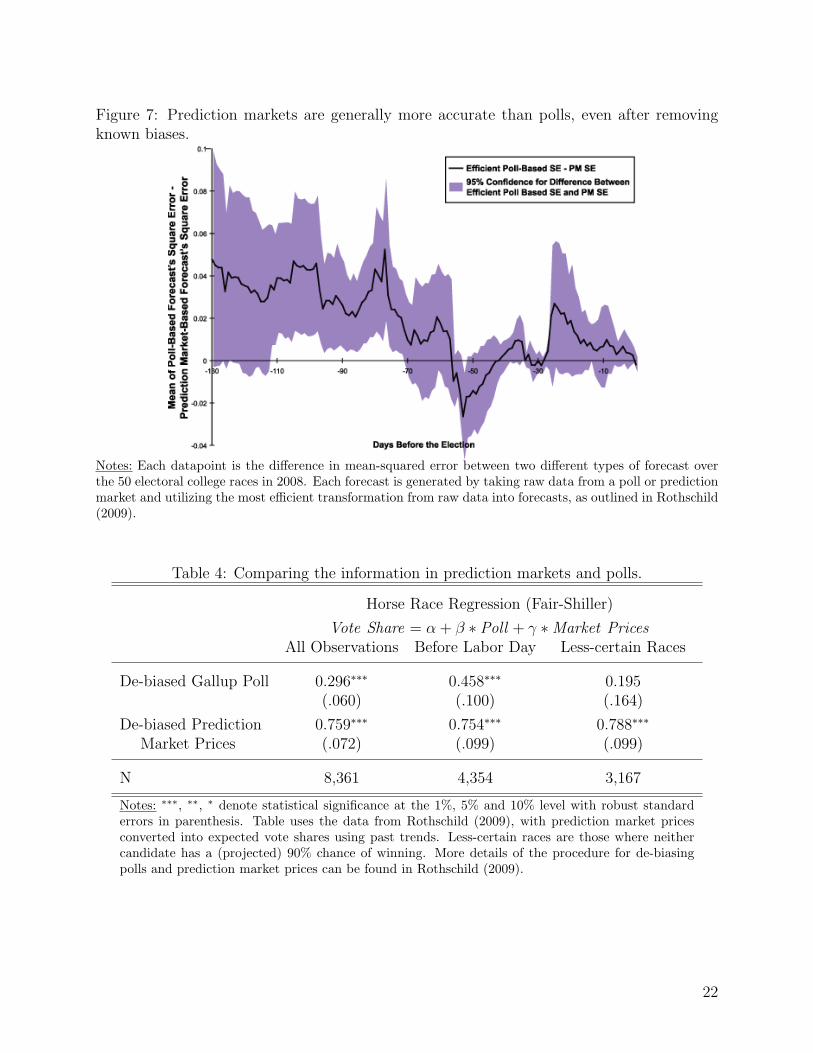
Figure 7: Prediction markets are generally more accurate than polls, even after removingknown biases.
Notes: Each datapoint is the difference in mean-squared error between two different types of forecast overthe 50 electoral college races in 2008. Each forecast is generated by taking raw data from a poll or predictionmarket and utilizing the most efficient transformation from raw data into forecasts, as outlined in Rothschild(2009).
Table 4: Comparing the information in prediction markets and polls.
Horse Race Regression (Fair-Shiller)
Vote Share = α + β ∗ Poll + γ ∗ Market PricesAll Observations Before Labor Day Less-certain Races
De-biased Gallup Poll 0.296∗∗∗ 0.458∗∗∗ 0.195(.060) (.100) (.164)
De-biased Prediction 0.759∗∗∗ 0.754∗∗∗ 0.788∗∗∗
Market Prices (.072) (.099) (.099)
N 8,361 4,354 3,167
Notes: ∗∗∗, ∗∗, ∗ denote statistical significance at the 1%, 5% and 10% level with robust standarderrors in parenthesis. Table uses the data from Rothschild (2009), with prediction market pricesconverted into expected vote shares using past trends. Less-certain races are those where neithercandidate has a (projected) 90% chance of winning. More details of the procedure for de-biasingpolls and prediction market prices can be found in Rothschild (2009).
22

Hewlett-Packard to forecast important variables like quarterly printer sales. These results
showed that the markets were more accurate than the company’s official forecasts. This
improvement in accuracy was obtained even though the markets had closed, and final prices
were known, at the time the official forecast was made.
Second, Cowgill, Wolfers and Zitzewitz (2009) analyze data from 270 markets run inside
of Google. While the markets were, in general, quite accurate, and often provided fore-
casts that would have been difficult to obtain in anything other than an ad hoc way, there
were identifiable biases in some market prices. In particular, when markets involved the
performance of Google as a company, optimistic outcomes were forecast to be more likely
to happen than they actually were. Moreover, this “optimistic bias” was more pronounced
among traders who were newer employees, and on days when Google’s stock appreciated.
Third, and finally, Berg, Neumann and Rietz (2009) ran several prediction markets to
predict Google’s market cap at the end of the first day of trading. Notably, these prediction
could be compared to the auction that Google used in setting its IPO price. The prediction
market fared quite well: its prediction was 4% above the actual market cap, while the IPO
price was 15% below. Had the company set its IPO price based on the prediction market
price, they would have earned $225 million more in their IPO.
5 Discovering Economic Models
Tthe information from prediction markets has also proven quite useful in augmenting event
studies (Snowberg, Wolfers and Zitzewitz, 2011). This use of prediction markets may be
of particular interest to economic forecasters, as they reveal pieces of the economic model
underlying the markets’ reaction to various types of information. We show first how predic-
tion markets can be used to measure the uncertainty surrounding an event, before exploring
two examples of prediction market event studies. The first example measures the expected
impact of the second Iraq war on oil prices, while the second example examines the impact
23
of politics on broad stock market indices.
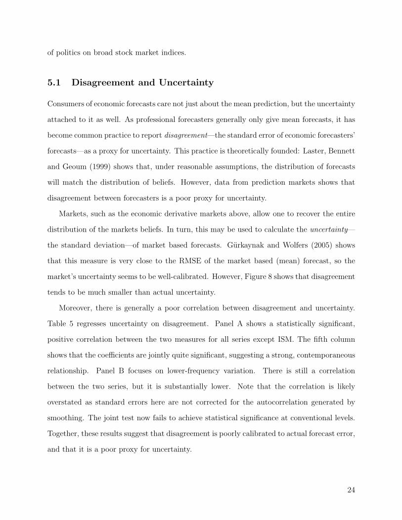
5.1 Disagreement and Uncertainty
Consumers of economic forecasts care not just about the mean prediction, but the uncertainty
attached to it as well. As professional forecasters generally only give mean forecasts, it has
become common practice to report disagreement—the standard error of economic forecasters’
forecasts—as a proxy for uncertainty. This practice is theoretically founded: Laster, Bennett
and Geoum (1999) shows that, under reasonable assumptions, the distribution of forecasts
will match the distribution of beliefs. However, data from prediction markets shows that
disagreement between forecasters is a poor proxy for uncertainty.
Markets, such as the economic derivative markets above, allow one to recover the entire
distribution of the markets beliefs. In turn, this may be used to calculate the uncertainty—
the standard deviation—of market based forecasts. Gurkaynak and Wolfers (2005) shows
that this measure is very close to the RMSE of the market based (mean) forecast, so the
market’s uncertainty seems to be well-calibrated. However, Figure 8 shows that disagreement
tends to be much smaller than actual uncertainty.
Moreover, there is generally a poor correlation between disagreement and uncertainty.
Table 5 regresses uncertainty on disagreement. Panel A shows a statistically significant,
positive correlation between the two measures for all series except ISM. The fifth column
shows that the coefficients are jointly quite significant, suggesting a strong, contemporaneous
relationship. Panel B focuses on lower-frequency variation. There is still a correlation
between the two series, but it is substantially lower. Note that the correlation is likely
overstated as standard errors here are not corrected for the autocorrelation generated by
smoothing. The joint test now fails to achieve statistical significance at conventional levels.
Together, these results suggest that disagreement is poorly calibrated to actual forecast error,
and that it is a poor proxy for uncertainty.
24

Figure 8: Uncertainty is generally greater than disagreement.
20
40
60
80
100
120
7/02 7/03 7/04 7/05
Non−Farm Payrolls
.5
1
1.5
2
2.5
7/02 7/03 7/04 7/05
Business Confidence (ISM)
.1
.2
.3
.4
.5
.6
7/02 7/03 7/04 7/05
Retail Sales (excluding Autos)
0
5
10
15
20
7/02 7/03 7/04 7/05
Initial Unemployment Claims
Sta
ndar
d D
evia
tion
Date of Data Release
Uncertainty: Standard Deviation of Market−Based PDF
Disagreement: Standard Deviation of Estimates Among MMS Forecasters
Notes: Dashed lines show 5-period, centered, moving averages. Adapted from Gurkaynak and Wolfers (2005).
5.2 War
Wars can have large economic impacts, and, in the post WWII era, usually have a fairly
long buildup. However, as each war is unique, it is difficult to build wars into economic
forecasts, even when the probability of war is very high. In particular, it is quite difficult to
make conditional forecasts in anything other than an ad hoc way, as much of the information
available may be tainted by political considerations, and, moreover, such a large-scale event
may have general equilibrium effects that are poorly understood.
Prediction market event studies present the possibility of improving economic forecasts
when such a unique event becomes likely. By tracking the probability of such an event
through a prediction market, and correlating movements in the prediction market with asset
prices, it becomes possible to understand the market’s assessment of how such an event will
affect outcomes such as the price of oil, or the returns to securities.
Leigh, Wolfers and Zitzewitz (2003) performed a prediction market event study in the
25

Table 5: Disagreement among forecasters is a poor proxy for uncertainty.
Business Retail JointNon-farm confidence sales Significancepayrolls (ISM) (ex Autos) (F-test)
Panel A: Contemporaneous Relationship
Uncertainty t = α + β ∗ Disagreement t
Disagreement 0.66∗∗ -0.03 0.44∗∗ 0.27∗∗∗
p = .0002(.29) (.12) (.16) (.07)
Constant 73.6∗∗∗ 2.04∗∗∗ 0.36∗∗∗ 10.86∗∗∗
(10.39) (.13) (.03) (.47)
Adjusted R2 0.11 -0.03 0.20 0.17
Panel B: Low Frequency—5 Period, Centered, Moving Averages
Smoothed Uncertainty t = α + β ∗ Smoothed Disagreement t
Disagreement 0.55 0.10 0.65∗∗ .32∗∗
p = .15(.47) (.10) (.24) (.06)
Constant 77.7∗∗∗ 1.89∗∗∗ 0.32∗∗∗ 10.5∗∗∗
(16.8) (.11) (.05) (.37)
Adjusted R2 0.01 -0.002 0.23 0.32
Notes: ∗∗∗, ∗∗, ∗ denote statistically significant regression coefficients at the 1%, 5% and 10% level withstandard errors in parenthesis. Adapted from Table 5 in Gurkaynak and Wolfers (2005).
buildup to the second Iraq war. Its prospective analysis showed that every 10% increase in
the probability of war lead to a $1 increase in the spot price of oil. As shown in Figure 9, they
used a prediction market, run by Intrade.com, that measured the probability that Saddam
Hussein would be out of office by a certain date as the probability of war a few months before
that date.16 As can be seen from the figure, as the probability of war fluctuated, so did the
spot price of oil.
Moreover, the S&P 500 dropped 1.5% for every 10% increase in the probability of war.
This implied that the market anticipated that a war would decrease stock prices by 15
16This is a reasonable proxy—out of office was defined as no longer controlling the center of Baghdad.
26

Figure 9: Response of oil prices to the probability of war.
Oil Price(LHS)
Probability Saddam Oustedby June 2003 (RHS)
Redemption Yield on PDVSA (Venezuela)corporate bonds (RHS)
00
25%
50%
75%
100%
$16
$21
$26
$31
$36
Oil
Pri
ce (
Wes
t T
exas
In
term
edia
te,
$/B
arre
l)
01 Oct 02 01 Nov 02 01 Dec 02 01 Jan 03 01 Feb 03
Notes: Adapted from Leigh, Wolfers and Zitzewitz (2003).
Figure 10: Predicted distributions of the S&P 500 for various probabilities of war.
0.0
00
0.0
05
0.0
10
0.0
15
Sta
te P
rice
500 600 700 800 900 1000 1100 1200 1300 1400Strike Price (S&P 500)
Peace (0%)
Low War Risk (40%)
High War Risk (80%)
War (100%)
Notes: Adapted from Wolfers and Zitzewitz (2008b).
27

percentage points. A further analysis of S&P 500 options revealed that the distribution of
potential outcomes was quite negatively skewed. Option prices suggested there was a 70%
probability that war would have a moderately negative effect of 0 to -15 percentage points,
a 20% probability of a -15 to -30 percentage-point effect, and a 10% chance of even larger
declines. Figure 10 presents this information in a slightly disaggregated way: for each of four
probabilities of war, it shows the full state-price distribution. It is clear that in the case of
certain war (the thick, solid line), the mode of the state-price distribution is substantially
shifted from what it would be under a zero chance of war (the thin, dashed line). Moreover,
in certain war, the markets predicted a non-negligible probability that the S&P 500 would
fall below 500 (Wolfers and Zitzewitz, 2008b).
The striking magnitude of this effect stands in contrast with the conventional wisdom,
based in part on studies such as Cutler, Poterba and Summers (1989), that political and
military news explain only a small portion of market movements. In contrast, Wolfers and
Zitzewitz (2008b) finds that, “[O]ver 30% of the variation in the S&P and 75% of the variation
in spot oil prices between September 2002 and February 2003 can be explained econometri-
cally by changes in the probability of war (and, for oil, the Venezuelan crisis).” The authors
note that it is possible to reconcile this result with the conventional wisdom by noting that
typically when economically important events happen, they are often near certainties. That
is to say, if the actual declaration of war comes when the market’s assessment of the prob-
ability of war is already 95%, then any correlated market movements must be scaled by a
factor of 20 to appreciate the full economic magnitude of the event. However, determining
the markets’ assessment of the probability of war immediately preceding an event is quite
difficult without prediction markets.
Additionally, prediction markets can be constructed to measure the overall economic cost
of a military intervention. For example, to determine the state price distribution of the S&P
500, a researcher could combine S&P 500 futures with a prediction market on the probability
of war, as shown in Figure 10. A cleaner design would be to issue options on the S&P 500
28

that pay off only if the U.S. has gone to war, with all transactions reversed if the U.S. does
not go to war. By combining these options with prediction markets tied directly to whether
or not the U.S. goes to war, and, for example, the level of troop deployments in the case
of war, one could recover state price distributions under different military scenarios. This
(largely theoretical) use of prediction markets has been described as “decision markets” or,
more spectacularly, “futarchy” (Hanson, 1999; Berg and Rietz, 2003; Hahn and Tetlock,
2005; Hanson, 2011).17
5.3 Politics
Prediction markets can also help to determine the effect of more routine political events,
such as elections. A large literature in political science, economics, and the popular press
argues about the effect of various candidates and parties, and the policies they endorse,
on the economy. Despite some evidence that broad stock market indices in the U.S. may
perform up to 20% better under Democrats than Republicans (Santa-Clara and Valkanov,
2003), political considerations are rarely reflected in economic forecasts.
This is at least partly due to the fact that there is no academic consensus on even the
direction of the effect of political outcomes on economic variables. However, markets exhibit
much more consistency. In particular, by using a prediction market event study on election
night 2004, Snowberg, Wolfers and Zitzewitz (2007a) shows that broad stock market indices
rose approximately 2% on news of Bush’s victory over Kerry. Moreover, this effect seems to
be relatively consistent across time, as, using data from 1880-2004, the same authors show
that a Republican victory caused a broad-based market index to rise by approximately 2.5%.
Figure 11 shows the price of a prediction market that paid off if Bush won in 2004,
expressed as risk-neutral probabilities, and the value of a near-month S&P 500 future over
election night 2004. The prices of these two securities track each other quite closely. The
probability of Bush’s re-election starts near 55%, and declines by about 30% on flawed exit
17Malhotra and Snowberg (2009) provide an example of how to use a decision market to pick the presi-dential candidate that would maximize a particular party’s chance of winning.
29

Figure 11: Prediction markets uncover the market’s reaction to political changes.
1115
1120
1125
1130
1135
1140
1145
1150
1155
S&
P 5
00 F
utu
re
0
25
50
75
100
InT
rade:
Pro
bab
ilit
y B
ush
Re−
elec
ted
Election Day Post−election Day12 noon 3 p.m. 6 p.m. 9 p.m. Midnight 3 a.m. 6 a.m.
Time, EST
Probability Bush wins Presidency (InTrade)
S&P Future, Delivery Date 12/2004 (CME)
Notes: Adapted from Snowberg, Wolfers and Zitzewitz (2007a).
polls showing Kerry with a lead in some swing states. At approximately the same time,
the S&P 500 future decreases in value by approximately 0.7%. Thus, this particular event
study indicates that a Bush victory would increase the value of the S&P 500 by 0.7%/30%
= 2.3%. As early vote totals were released, showing the faults of the earlier poll results,
Bush’s probability of re-election climbed 65%, and the S&P rose by about 1.3%. Thus, this
event study indicates that a Bush victory would increase the S&P 500 by 1.3%/65% = 2%.
A first differences regression essentially averages together a large number of event studies.
In particular, estimates of
∆(log(Financial Variablet)) = α + β∆(Re − election Probabilityt) + εt
are shown for a number of different financial variables in Table 6. Estimates based on 10-
minute and 30-minute differences are consistent, although the results based on 30-minute
differences have slightly larger coefficients, reflecting the fact that the prediction market was
30

Table 6: High-frequency data from prediction markets allows for precise estimates of theeffect of elections on economic variables.
10-Minute First Differences 30-Minute First Differences
Estimated Effect ofn
Estimated Effect ofn
Bush Presidency Bush Presidency
Dependent Variable: ∆(Log(Financial Index))
S&P 500 0.015∗∗∗ 104 0.021∗∗∗ 35(.004) (.005)
Dow Jones Industrial Average 0.014∗∗∗ 84 0.021∗∗∗ 29(.005) (.006)
Nasdaq 100 0.017∗∗∗ 104 0.024∗∗∗ 35(.006) (.008)
U.S. Dollar 0.004 93 0.005∗∗ 34(vs. Trade-weighted basket) (.003) (.003)
Dependent Variable: ∆(Price)
December ’04 1.110∗∗∗ 88 1.706∗∗∗ 29Light (.371) (.659)Crude Oil December ’05 0.652∗ 85 1.020 28Futures (.375) (.610)
December ’06 -0.580 63 -0.666 21(.783) (.863)
Dependent Variable: ∆(Yield)
2-Year T-Note Future 0.104∗ 84 0.108∗∗∗ 30(.058) (.036)
10-Year T-Note Future 0.112∗∗ 91 0.120∗∗ 31(.050) (.046)
Notes: ∗∗∗, ∗∗, ∗ denote statistically significant regression coefficients at the 1%, 5% and 10% level withrobust standard errors in parenthesis. The sample period is noon Eastern Time on 11/2/2004 to sixa.m. on 11/3/2004. Election probabilities are the most recent transaction prices, collected every tenminutes from InTrade.com (then TradeSports.com), S&P, Nasdaq, and foreign exchange futures are fromthe Chicago Mercantile Exchange; Dow and bond futures are from the Chicago Board of Trade, whileoil futures data are from the New York Mercantile Exchange. Equity, bond and currency futures haveDecember 2004 delivery dates. Yields are calculated for the Treasury futures using the daily yieldsreported by the Federal Reserve for 2- and 10-year Treasuries, and projecting forward and backwardfrom the bond market close at 3 p.m. using future price changes and the future’s durations of 1.96 and7.97 reported by CBOT. The trade-weighted currency portfolio includes six currencies with CME-tradedfutures (the Euro, Yen, Pound, Australian and Canadian Dollars, and the Swiss Franc). Adapted fromTable 1 in Snowberg, Wolfers and Zitzewitz (2007a).
31

slower to incorporate information than financial markets, as is apparent from Figure 11. As
can be seen from the table, a Bush victory increased all three major US stock indices by
2–2.5%. Consistent with expectations of expansionary fiscal policies, the Dollar and Bond
Yields rose, as did near-term expectations of the price of oil.
Were this just a one-off result, it would make little sense to add political changes to a
forecasting model. However, as Figure 12 and Table 7 show, Republican elections routinely
lead to an increase of about 2.5% in a broad equity market index. The first panel of the
figure, and first column of the table, show the relationship between the change in probability
of a Republican President over election night and the change in a broad-based market index
from market close the day before the election, to market close the day after.18 That is, the
table contains an estimate of:
∆(Market Indext) = α + β∆(Republican Presidentt) + εt
where ∆(Republican Presidentt) = I(Republican Presidentt) − P (Republican Electiont)
where I(Republican Electedt) takes a value of one if a Republican was elected in year t, and
zero otherwise, and P (Republican Electiont) is the expected probability of a Republican
victory, according to the price of an historical prediction market (from Rhode and Strumpf,
2004) the night before the election.
The second panel of the figure, and second column of the table, show the role of prediction
markets in this estimate. Lacking prediction market data, Santa-Clara and Valkanov (2003)
simply fix P (Republican Electiont) = 0.5 for all years from which they have data: 1928–1996.
This results in the smaller, statistically insignificant estimate found in the second column
of Table 7. The third column of the same table contains data from all years available in
Snowberg, Wolfers and Zitzewitz (2007a), and shows a precisely estimated, stable effect of
18Equity index values are from Schwert’s (1990) daily equity returns data, which attempts to replicatereturns on a value-weighted total return index, supplemented by returns on the CRSP-value-weighted port-folio since 1962. The prediction market prices come from the curb exchange on Wall Street, where exchangeson various political candidates ran up until shortly after WWII (Rhode and Strumpf, 2004).
32

Figure 12: Prediction markets uncover the market’s reaction to political changes.
Hoover−1928
Roosevelt−1932
Roosevelt−1936
Roosevelt−1940
Roosevelt−1944
Truman−1948
Eisenhower−1952
Eisenhower−1956
Kennedy−1960
Johnson−1964Nixon−1968
Nixon−1972
Carter−1976
Reagan−1980
Reagan−1984
Bush−1988
Clinton−1992
Clinton−1996
−.04
−.02
0
.02
−1 −.75 −.5 −.25 0 .25 .5 .75 1Change in Probability of a Republican President
I(Republican President) − Pre−election prediction market price
Estimating Market Response using Prediction Markets
Hoover−1928
Roosevelt−1932
Roosevelt−1936
Roosevelt−1940
Roosevelt−1944
Truman−1948
Eisenhower−1952
Eisenhower−1956
Kennedy−1960
Johnson−1964Nixon−1968
Nixon−1972
Carter−1976
Reagan−1980
Reagan−1984
Bush−1988
Clinton−1992
Clinton−1996
−.04
−.02
0
.02
−1 −.75 −.5 −.25 0 .25 .5 .75 1Change in Probability of a Republican President
I(Republican President) − 0.5
Estimating Market Response: Equal Probability Assumption
Ch
ang
e in
Val
ue−
wei
gh
ted I
nd
ex:
Pre
−el
ecti
on
clo
se t
o P
ost
−el
ecti
on c
lose
Notes: Adapted from Snowberg, Wolfers and Zitzewitz (2011).
33

Table 7: Prediction markets identify the effect of elections on markets.
Dependent Variable:Stock returns from election-eve
close to post-election close
∆P (Republican President) 0.0297∗∗ 0.0249∗∗∗
(From Prediction Markets) (.118) (.0082)
I(Republican President) − 0.5 0.0128(As in Santa-Clara and Valkanov) (.0089)
Constant -0.0102 -0.0027 0.0014(.0059) (0.0040) (0.0028)
Sample 1928–1996 1928–1996 1880–2004N 18 18 32
Notes: ∗∗∗, ∗∗, ∗ denote statistical significance at the 1%, 5% and 10% level with robust standarderrors in parenthesis. Adapted from Table 5 in Snowberg, Wolfers and Zitzewitz (2007a).
the election of a Republican president of about 2.5%. The contribution of prediction markets
is clear: a more precise estimate of the probability of one or the other candidate winning
allows for a better estimate of the effect of political candidates on financial markets.
6 Conclusion
Over the last half decade, many economists, and the public, have re-evaluated the efficiency
of financial markets. While these re-evaluations have not been favorable to markets, it is
important to keep in mind the alternative (Zingales, 2010). In the case of forecasting, the
alternative is often professional forecasters, polls, pundits, or a combination of the three. As
we have shown in these paper, prediction markets out-perform both professional forecasters
and polls in a variety of statistical tests.
We have shown that prediction markets have many of the properties expected under the
efficient markets hypothesis. In particular, they are difficult to manipulate, lack significant
arbitrage opportunities, aggregate information quickly and in a seemingly efficient manner.
34

Evidence of efficiency can be seen in the macro-derivatives markets, which out-perform pro-
fessional forecasters, or in political prediction markets, which out-perform polls.
However, prediction markets are not a panacea. In particular, care must be taken when
designing prediction markets to ensure they are interesting, well-specified, and are not subject
to excessive insider information. More pernicious problems come from behavioral biases,
such as those underlying the favorite-longshot bias, and knowing when there is dispersed
information that can be aggregated.
With that said, we believe the real promise of prediction markets comes not from their
ability to predict particular events. Rather, the real promise lies in using these markets,
often several at a time, to test particular economic models, and use these models to improve
economic forecasts.
35

References
Abramowicz, Michael. 2007. “The Hidden Beauty of the Quadratic Market Scoring Rule:A Uniform Liquidity Market Maker, with Variations.” The Journal of Prediction Markets1(2):111–125.
Alquist, Ron and Robert J. Vigfusson. 2012. Forecasting Oil Prices. In Handbook of EconomicForecasting, Volume 2. Elsevier: Handbooks in Economics series.
Arrow, Kenneth J., Robert Forsythe, Michael Gorham, Robert Hahn, Robin Hanson, John O.Ledyard, Saul Levmore, Robert Litan, Paul Milgrom, Forrest D. Nelson, George R.Neumann, Marco Ottaviani, Thomas C. Schelling, Robert J. Shiller, Vernon L. Smith,Erik Snowberg, Cass R. Sunstein, Paul C. Tetlock, Philip E. Tetlock, Hal R. Varian,Justin Wolfers and Eric Zitzewitz. 2008. “The Promise of Prediction Markets.” Science320(5878):877–878.
Bakshi, Gurdip and Dilip Madan. 2000. “Spanning and Derivative-Security Valuation.”Journal of Financial Economics 55(2):205–238.
Bell, Tom W. 2009. “Private Prediction Markets and the Law.” The Journal of PredictionMarkets 3(1):89–110.
Berg, Henry and Todd A. Proebsting. 2009. “Hanson’s Automated Market Maker.” TheJournal of Prediction Markets 3(1):45–59.
Berg, Joyce E., George R. Neumann and Thomas A. Rietz. 2009. “Searching for Google’sValue: Using Prediction Markets to Forecast Market Capitalization Prior to an InitialPublic Offering.” Management Science 55(3):348–361.
Berg, Joyce E. and Thomas A. Rietz. 2003. “Prediction Markets as Decision Support Sys-tems.” Information Systems Frontiers 5(1):79–93.
Berg, Joyce E. and Thomas A. Rietz. 2006. The Iowa Electronic Market: Lessons Learnedand Answers Yearned. In Information Markets: A New Way of Making Decisions in thePublic and Private Sectors, ed. Robert Hahn and Paul Tetlock. Washington, D.C.: AEI-Brookings Joint Center.
Berg, Joyce, Nelson Forrest and Thomas Rietz. 2006. “Accuracy and Forecast StandardError in Prediction Markets.” University of Iowa, mimeo.
Berg, Joyce, Robert Forsythe, Forrest Nelson and Thomas Rietz. 2008. Results from a DozenYears of Election Futures Markets Research. In The Handbook of Experimental EconomicsResults, ed. Charles R. Plott and Vernon L. Smith. Elsevier: Handbooks in Economicsseries.
Camerer, Colin F. 1998. “Can Asset Markets be Manipulated? A Field Experiment withRacetrack Betting.” Journal of Political Economy 106(3):457–482.
36

Carr, Peter and Dilip Madan. 2001. “Optimal Positioning in Derivative Securities.” Quan-titative Finance 1(1):19–37.
Chen, Kay-Yut and Charles R. Plott. 2002. “Information Aggregation Mechanisms: Con-cept, Design and Implementation for a Sales Forecasting Problem.” California Institute ofTechnology Social Science Working Paper #1131.
Chen, Kay-Yut and Marina Krakovsky. 2010. Secrets of the Moneylab: How BehavioralEconomics Can Improve Your Business. Portfolio / Penguin.
Cowgill, Bo, Justin Wolfers and Eric Zitzewitz. 2009. “Using Prediction Markets to TrackInformation Flows: Evidence from Google.” Dartmouth College, memeo.
Cutler, David M., James M. Poterba and Lawrence H. Summers. 1989. “What Moves StockPrices?” Journal of Portfolio Management 15(3):4–12.
Dahan, Ely, Arina Soukhoroukova and Martin Spann. 2010. “New Product Development 2.0:Preference Markets—How Scalable Securities Markets Identify Winning Product Conceptsand Attributes.” Journal of Product Innovation Management 27(7):937–954.
Diebold, Francis X. and Robert S. Mariano. 1995. “Comparing Predictive Accuracy.” Journalof Business and Economic Statistics 13(3):134–144.
Duffee, Gregory. 2012. Forecasting Interest Rates. In Handbook of Economic Forecasting,Volume 2, ed. Allan Timmermann and Graham Elliott. Elsevier: Handbooks in Economicsseries.
Erikson, Robert S. and Christopher Wlezien. 2008. “Are Political Markets Really Superiorto Polls as Election Predictors?” Public Opinion Quarterly 72(2):190–215.
Fair, Ray C. and Robert J. Shiller. 1990. “Comparing Information in Forecasts from Econo-metric Models.” American Economic Review 80(3):375–389.
Gaspoz, Cedric. 2011. Prediction Markets Supporting Technology Assessment. Self-published.
Gjerstad, Steven. 2005. “Risk Aversion, Beliefs, and Prediction Market Equilibrium.” Uni-versity of Arizona, mimeo.
Gurkaynak, Refet and Justin Wolfers. 2005. Macroeconomic Derivatives: An Initial Analysisof Market-Based Macro Forecasts, Uncertainty, and Risk. In NBER International Seminaron Macroeconomics 2005, ed. Jeffrey A. Frankel and Christopher A. Pissarides. Cambridge,MA: MIT Press pp. 11–50.
Hahn, Robert W. and Paul C. Tetlock. 2005. “Using Information Markets to Improve PublicDecision Making.” Harvard Journal of Law and Public Policy 28:213–289.
Hanson, R. 2007. “Logarithmic Market Scoring Rules for Modular Combinatorial Informa-tion Aggregation.” The Journal of Prediction Markets 1(1):3–15.
Hanson, Robin. 1999. “Decision Markets.” IEEE Intelligent Systems 14(3):16–19.
37

Hanson, Robin. 2003. “Combinatorial Information Market Design.” Information SystemsFrontiers 5(1):107–119.
Hanson, Robin. 2011. “Shall we Vote on Values, but Bet on Beliefs?” Journal of PoliticalPhilosophy forthcoming.
Hanson, Robin, Ryan Opera, David Porter, Chris Hibbert and Dorina Tila. 2011. “CanManipulators Mislead Prediction Market Observers?” George Mason University, mimeo.
Hanson, Robin and Ryan Oprea. 2009. “A Manipulator Can Aid Prediction Market Accu-racy.” Economica 76(302):304–314.
Hanson, Robin, Ryan Oprea and David Porter. 2006. “Information Aggregation and Ma-nipulation in an Experimental Market.” Journal of Economic Behavior & Organization60(4):449–459.
Harvey, David I., Stephen J. Leybourne and Paul Newbold. 1998. “Tests for Forecast En-compassing.” Journal of Business & Economic Statistics 16(2):254–259.
Hausch, Donald and William Ziemba, eds. 2007. Handbook of Sports and Lottery Markets.Elsevier: Handbooks in Finance series.
Jullien, Bruno and Bernard Salanie. 2000. “Estimating Preferences Under Risk: The Caseof Racetrack Bettors.” Journal of Political Economy 108(3):503–530.
Laster, D., P. Bennett and In Sun Geoum. 1999. “Rational Bias in Macroeconomic Fore-casts.” Quarterly Journal of Economics 114(1):293–318.
Lavoie, Jim. 2009. “The Innovation Engine at Rite-Solutions: Lessons From the CEO.”Journal of Prediction Markets 3(1):1–11.
Leigh, Andrew, Justin Wolfers and Eric Zitzewitz. 2003. “What do Financial Markets Thinkof the War with Iraq?” NBER Working Paper #9587 .
Leitch, Gordon and J. Ernest Tanner. 1991. “Economic Forecast Evaluation: Profits Versusthe Conventional Error Measures.” The American Economic Review 81(3):580–590.
Malhotra, Neil and Erik Snowberg. 2009. “The 2008 Presidential Primaries through the Lensof Prediction Markets.” California Institute of Technology, mimeo.
Manski, Charles F. 2006. “Interpreting the Predictions of Prediction Markets.” EconomicsLetters 91(3):425–429.
Marinovic, Ivan, Marco Ottaviani and Peter Norman Sørenson. 2011. Modeling Idea Markets:Between Beauty Contests and Prediction Markets. In Prediction Markets, ed. LeightonVaughn Williams. Routledge.
Ottaviani, Marco and Peter N. Sørensen. 2010. “Aggregation of Information and Beliefs:Asset Pricing Lessons from Prediction Markets.” Northwestern University, mimeo.
38

Ottaviani, Marco and Peter Norman Sørenson. 2012. Forecasters’ Objectives and Strategies.In Handbook of Economic Forecasting, Volume 2. Elsevier: Handbooks in Economicsseries.
Plott, Charles R. 2000. “Markets as Information Gathering Tools.” Southern EconomicJournal 67(1):2–15.
Plott, Charles R. and Shyam Sunder. 1982. “Efficiency of Experimental Security Marketswith Insider Information: An Application of Rational-Expectations Models.” The Journalof Political Economy 90(4):663–698.
Plott, Charles R. and Shyam Sunder. 1988. “Rational Expectations and the Aggregation ofDiverse Information in Laboratory Security Markets.” Econometrica pp. 1085–1118.
Rhode, Paul W. and Koleman S. Strumpf. 2004. “Historical Presidential Betting Markets.”Journal of Economic Perspectives 18(2):127–142.
Rhode, Paul W. and Koleman S. Strumpf. 2008. “Historical Election Betting Markets: AnInternational Perspective.” University of Arizona, mimeo.
Rothschild, David. 2009. “Forecasting Elections Comparing Prediction Markets, Polls, andTheir Biases.” Public Opinion Quarterly 73(5):895–916.
Rubinstein, Mark. 1994. “Implied Binomial Trees.” Journal of Finance 69(3):771–818.
Santa-Clara, Pedro and Rossen Valkanov. 2003. “The Presidential Puzzle: Political Cyclesand the Stock Market.” The Journal of Finance 58(5):1841–1872.
Schwert, G. William. 1990. “Indexes of U.S. Stock Prices from 1802-1987.” Journal ofBusiness 63(3):399–426.
Servan-Schreiber, Emile, Justin Wolfers, David M. Pennock and Brian Galebach. 2004. “Pre-diction Markets: Does Money Matter?” Electronic Markets 14(3):243–251.
Snowberg, Erik and Justin Wolfers. 2010. “Explaining the Favorite-Longshot Bias: Is itRisk-Love or Misperceptions?” Journal of Political Economy 118(4):723–746.
Snowberg, Erik, Justin Wolfers and Eric Zitzewitz. 2005. Information (In)efficiency in Predic-tion Markets. In Information Efficiency in Betting Markets, ed. Leighton Vaughn Williams.Cambridge Unversity Press pp. 366–386.
Snowberg, Erik, Justin Wolfers and Eric Zitzewitz. 2007a. “Partisan Impacts on the Econ-omy: Evidence from Prediction Markets and Close Elections.” The Quarterly Journal ofEconomics 122(2):807–829.
Snowberg, Erik, Justin Wolfers and Eric Zitzewitz. 2007b. Prediction Markets: From Politicsto Business (and Back). In Handbook of Sports and Lottery Markets, ed. Donald Hauschand William Ziemba. Elsevier: Handbooks in Finance series pp. 385–402.
39

Snowberg, Erik, Justin Wolfers and Eric Zitzewitz. 2011. How Prediction Markets can SaveEvent Studies. In Prediction Markets, ed. Leighton Vaughn Williams. Routledge.
Spears, Brian, Christina LaComb, John Interrante, Janet Barnett and Deniz Senturk-Dogonaksoy. 2009. “Examining Trader Behavior in Idea Markets: An Implementationof GE’s Imagination Markets.” The Journal of Prediction Markets 3(1):17–39.
Strumpf, Koleman S. 2009. “Introduction to Special Issue on Corporate Applications ofPrediction Markets.” Journal of Prediction Markets 3(1):i–vii.
Tetlock, Paul. 2004. “How Efficient Are Information Markets? Evidence from an OnlineExchange.” Columbia University, mimeo.
Tompkins, Robert G., William T. Ziemba and Stewart D. Hodges. 2008. The Favorite-Longshot Bias in S&P 500 and FTSE 100 Index Futures Options: The Return to Bets andthe Cost of Insurance. In Handbook of Sports and Lottery Markets, ed. Donald B. Hauschand William T. Ziemba. Elsevier: Handbooks in Finance series.
Tziralis, George and Ilias Tatsiopoulos. 2007. “Prediction Markets: An Extended LiteratureReview.” The Journal of Prediction Markets 1(1):75–91.
Vaughn Williams, Leighton, ed. 2005. Information Efficiency in Betting Markets. CambridgeUnversity Press.
West, Kenneth D. 1996. “Asymptotic Inference About Predictive Ability.” Econometrica64(5):1067–1084.
West, Kenneth D. 2006. Forecast Evaluation. In Handbook of Economic Forecasting, ed.Graham Elliott, Clive W.J. Granger and Allan Timmermann. Vol. 1 Elsevier chapter 3,pp. 99–134.
Wolfers, Justin and Andrew Leigh. 2002. “Three Tools for Forecasting Federal Elections:Lessons From 2001.” Australian Journal of Political Science 37(2):223–240.
Wolfers, Justin and Eric Zitzewitz. 2004. “Prediction Markets.” Journal of Economic Per-spectives 18(2):107–126.
Wolfers, Justin and Eric Zitzewitz. 2006. “Interpreting Prediction Market Prices as Proba-bilities.” NBER Working Paper Series # 12200.
Wolfers, Justin and Eric Zitzewitz. 2008a. Prediction Markets in Theory and Practice. InThe New Palgrave Dictionary of Economics, Second Edition, ed. Larry Blume and StevenDurlauf. London: Palgrave.
Wolfers, Justin and Eric Zitzewitz. 2008b. “Using Markets to Inform Policy: The Case ofthe Iraq War.” Economica 76(302):225–250.
Wright, Jonathan and Jon Faust. 2012. Forecasting Inflation. In Handbook of EconomicForecasting, Volume 2, ed. Graham Elliott and Allan Timmermann. Elsevier: Handbooksin Economics series.
40

Zhou, Guofo and David Rapach. 2012. Forecasting Stock Returns. In Handbook of EconomicForecasting, Volume 2, ed. Allan Timmermann and Graham Elliott. Elsevier: Handbooksin Economics series.
Zingales, Luigi. 2010. “Learning to Live with Not-so-Efficient Markets.” Daedalus 139(4):31–40.
Zitzewitz, Eric. May 30, 2007. “Manipulation can Affect Prices.” MidasOracle.org,http://www.midasoracle.org/2007/05/30/manipulation-can-affect-prices/.
41