prediction of aerodynamic performance and noise production ... · pdf fileprediction of...
TRANSCRIPT

March 2015
PREDICTION OF AERODYNAMICPERFORMANCE AND NOISEPRODUCTION OF AXIAL FANS
Robin van de Vondervoort
Faculty of Engineering Technology (CTW)Chair of Engineering Fluid Dynamics (EFD)
Exam committee:prof. dr. ir. C.H. Venner (Chairman)dr. ir. N.P. Kruyt (Mentor)dr. ir. Y.H. Wijnanting. P. Holkers
DocumentnumberTS – 193

A thesis submitted for the degree ofMaster of Science
PREDICTION OF AERODYNAMICPERFORMANCE AND NOISE PRODUCTION OF
AXIAL FANS
Author:
Robin van de Vondervoort
March 2015
Exam committeeprof. dr. ir. C.H. Venner (Chairman)dr. ir. N.P. Kruyt (Mentor)dr. ir. Y.H. Wijnanting. P. Holkers
University of Twente.Faculty of Engineering TechnologyProgram Mechanical Engineering
Group of Engineering Fluid Dynamics


Abstract
Low-speed axial fans are employed in a wide variety of industries, mainly to displace large quantities ofair with a low pressure difference. An important constraint on the use of these fans is the noise emittedto the far-field. In applications like cooling towers and condensers, the axial fan forms an importantsource of noise.
The noise emitted by low-speed axial fans produced by Howden Netherlands mainly produce noise of abroadband nature. To reduce this emitted broadband noise, conventionally a large number of prototypeswere constructed and trial-and-error experiments were performed to design silent fans. This approach isvery time-consuming and expensive. Therefore, a prediction of the emitted noise levels of new designsusing computational fluid dynamics and computational aeroacoustics is preferred. The objective of thisstudy is to investigate a suitable prediction technique for broadband aerodynamic noise, that can beapplied in a design process.
Most currently available methods for broadband noise prediction are based on computationally ex-pensive Large Eddy Simulations or Direct Numerical Simulation methods. The application of thesemethods is not (yet) feasible for the evaluation of numerous designs created in a design engineering pro-cess. The current study focuses on the applicability of a hybrid method, combining the computationallyless expensive Reynolds-averaged Navier-Stokes (RANS) method and the Stochastic Noise Generationand Radiation (SNGR) method.
The SNGR method has been validated in literature for cases like a car’s side mirror and an airfoiland slat configuration. The method is still in a development phase and constant improvements are in-troduced. The most recent extension is the application to rotating equipment. In this thesis the SNGRmethod was applied to rotating machinery in general and low-speed axial fans in particular for the firsttime.
To apply this method to an axial fan, the first step in this hybrid process is the prediction of theaerodynamic performance using a steady-state RANS computation, as incorporated in the commercialcomputational fluid dynamics package NUMECA FINE/Turbo. The results of this aerodynamic per-formance prediction are in good agreement with the experimental results, obtained at the Howden testfacility.
Using the results of the validated RANS computation as input, the second step is the reconstruc-tion of the turbulent velocity fluctuations with the SNGR method, incorporated in the NUMECAFINE/Acoustics FlowNoise module. This method stochastically reconstructs the turbulent noise sourcesconsistent with the Von Karman-Pao energy spectrum. Once these noise sources have been reconstructed,the propagation of noise through the fan duct is computed using a finite element acoustical method. Fi-nally, using a boundary element method radiation analysis, the sound pressure level at the far-fieldmicrophone is obtained.
A first preliminary result was obtained, by performing all steps necessary to reach a sound pressurelevel at a far-field microphone. A quantitative agreement with experimental results was not yet found,but various simplifications and assumptions have been applied in the current study. The impact of thesefactors has not been investigated yet. Therefore, further research is required to evaluate whether thehybrid SNGR approach is a suitable acoustics prediction method that can be incorporated in the designprocess of low-speed axial fans.
5

6
Acknowledgements
This report presents the final result for my Master Mechanical Engineering conducted at the Universityof Twente. It marks the end of an unforgettable and amazing period in my life. It would never havecome to this point, if it wasn’t for the help and support of a lot of people. I would like to take thisopportunity to thank some individuals in particular.
First of all, I would like to thank Niels Kruyt, my daily supervisor at the University of Twente duringthis final project. He was always available for questions and gave critical feed back if needed. Secondly,I would like to thank professor Harry Hoeijmakers, for inspiring me for the field of fluid dynamics inthe bachelor and guiding me throughout most of my master study. Next, I would like to thank all thepeople who have supported me in the complete process. Professor Hirschberg and professor Venner aregreatly acknowledged for steering the exploratory research in the beginning of the project into the rightdirection. For all the technical issues and questions I had, I would like to thank Wouter den Breeijenfor always helping me out swiftly. For all the valuable discussions and quick help I would like to thankRuben Verschoof, Marnix van Schrojenstein Lantman, Richard van der Sluis and Arjan Slaper.
This research would not have been possible without the valuable experimental input and practicalknowledge provided by Howden Netherlands. I would like to specifically thank Sander Venema and PeterHolkers of Howden Netherlands for our valuable discussions regarding the results and the possibility toattend the experiments at their test site.
The major part of the results provided in this thesis where obtained using software very kindlyprovided by NUMECA. Without their impeccable support department, the results presented in thisthesis would have never been obtained. In particular I would like to thank Colinda, Piere-Allain, Ervin,Paolo and especially Piergiorgio. The skype-meetings we had were sometimes lengthy, but in the end,very fruitful.
I would like to thank Carlijn, for supporting me through the complete project and motivating mewhen needed, but most of all, just for being her. Finally, I would like to thank my parents, for theunconditional support throughout my whole life and my time as a student.
RobinEnschede, March 2015
7

8
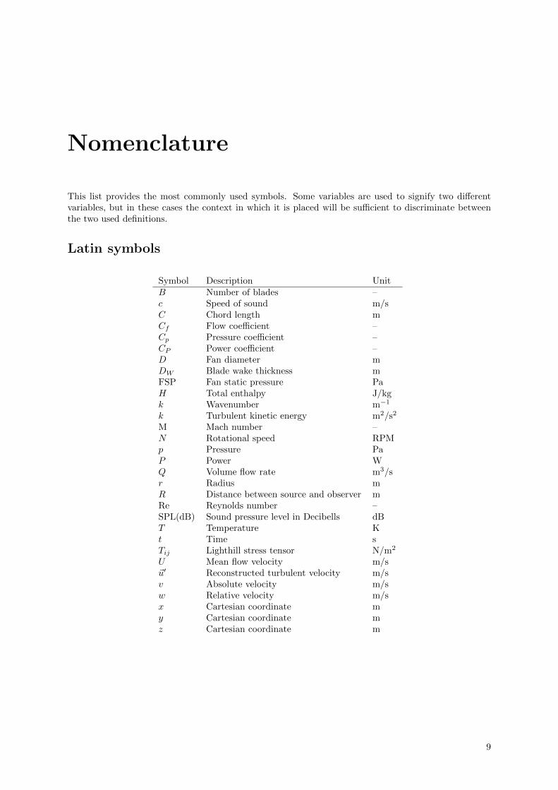
Nomenclature
This list provides the most commonly used symbols. Some variables are used to signify two differentvariables, but in these cases the context in which it is placed will be sufficient to discriminate betweenthe two used definitions.
Latin symbols
Symbol Description UnitB Number of blades –c Speed of sound m/sC Chord length mCf Flow coefficient –Cp Pressure coefficient –CP Power coefficient –D Fan diameter mDW Blade wake thickness mFSP Fan static pressure PaH Total enthalpy J/kgk Wavenumber m−1
k Turbulent kinetic energy m2/s2
M Mach number –N Rotational speed RPMp Pressure PaP Power WQ Volume flow rate m3/sr Radius mR Distance between source and observer mRe Reynolds number –SPL(dB) Sound pressure level in Decibells dBT Temperature Kt Time sTij Lighthill stress tensor N/m2
U Mean flow velocity m/s~u′ Reconstructed turbulent velocity m/sv Absolute velocity m/sw Relative velocity m/sx Cartesian coordinate my Cartesian coordinate mz Cartesian coordinate m
9

Greek symbols
Symbol Description Unitηts Total-to-static effiency –ηtt,q Quasi total-to-total efficiency –ηtt Total-to-total efficiency –µ Dynamic Viscosity Pa·sν Kinematic Viscosity m2/sω Rotational speed rad/sω Specific turbulent dissipation rate s−1
~ω Vorticity vector s−1
Π Sound power Wψ Phase angle radρ Density kg/m3
~σ Direction of Fourier component –ε Turbulent dissipation rate m2/s3
Subscripts
Symbol Description0 Total or mean flow quantity1 Condition at the fan inlet2 Condition at the fan outlet
avg Averaged valueh Condition at the hub
ref Reference levelrms Root mean square value
shaft Condition at the shaftt Condition at the blade tip
10

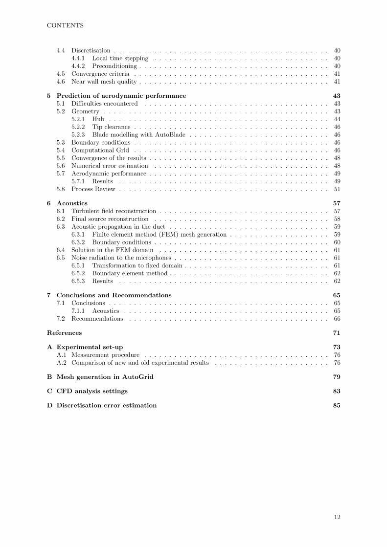
Contents
Abstract 5
Acknowledgements 7
Nomenclature 9
1 Introduction 131.1 Low-speed axial fans . . . . . . . . . . . . . . . . . . . . . . . . . . . . . . . . . . . . . . . 131.2 Aerodynamic performance . . . . . . . . . . . . . . . . . . . . . . . . . . . . . . . . . . . . 13
1.2.1 Dimensionless numbers . . . . . . . . . . . . . . . . . . . . . . . . . . . . . . . . . 141.3 Noise emission . . . . . . . . . . . . . . . . . . . . . . . . . . . . . . . . . . . . . . . . . . 161.4 Objective and outline . . . . . . . . . . . . . . . . . . . . . . . . . . . . . . . . . . . . . . 16
2 Literature Review 172.1 Sound and noise . . . . . . . . . . . . . . . . . . . . . . . . . . . . . . . . . . . . . . . . . 172.2 Noise perception . . . . . . . . . . . . . . . . . . . . . . . . . . . . . . . . . . . . . . . . . 172.3 Sources of sound . . . . . . . . . . . . . . . . . . . . . . . . . . . . . . . . . . . . . . . . . 18
2.3.1 Monopole sources . . . . . . . . . . . . . . . . . . . . . . . . . . . . . . . . . . . . . 182.3.2 Dipole sources . . . . . . . . . . . . . . . . . . . . . . . . . . . . . . . . . . . . . . 182.3.3 Quadrupole sources . . . . . . . . . . . . . . . . . . . . . . . . . . . . . . . . . . . 19
2.4 Lighthill’s analogy . . . . . . . . . . . . . . . . . . . . . . . . . . . . . . . . . . . . . . . . 202.4.1 Ffowcs Williams - Hawking method . . . . . . . . . . . . . . . . . . . . . . . . . . 212.4.2 Kirchhoff integral method . . . . . . . . . . . . . . . . . . . . . . . . . . . . . . . . 212.4.3 Required input . . . . . . . . . . . . . . . . . . . . . . . . . . . . . . . . . . . . . . 22
2.5 Sources of noise in axial flow fans . . . . . . . . . . . . . . . . . . . . . . . . . . . . . . . . 222.5.1 Broadband noise . . . . . . . . . . . . . . . . . . . . . . . . . . . . . . . . . . . . . 222.5.2 Discrete frequency noise . . . . . . . . . . . . . . . . . . . . . . . . . . . . . . . . . 222.5.3 Tip vortex – Tip clearance . . . . . . . . . . . . . . . . . . . . . . . . . . . . . . . 232.5.4 Noise in industry applications . . . . . . . . . . . . . . . . . . . . . . . . . . . . . . 23
2.6 Fukano model . . . . . . . . . . . . . . . . . . . . . . . . . . . . . . . . . . . . . . . . . . . 232.7 Stochastic Noise Generation and Radiation (SNGR) . . . . . . . . . . . . . . . . . . . . . 24
2.7.1 Damped Stochastic Noise Generation (DSNG) . . . . . . . . . . . . . . . . . . . . 262.7.2 Sound source reconstruction . . . . . . . . . . . . . . . . . . . . . . . . . . . . . . . 27
3 Benchmarks & Outline 293.1 Current benchmarks . . . . . . . . . . . . . . . . . . . . . . . . . . . . . . . . . . . . . . . 29
3.1.1 2D airfoil and slat configuration . . . . . . . . . . . . . . . . . . . . . . . . . . . . 293.1.2 3D Nozzle . . . . . . . . . . . . . . . . . . . . . . . . . . . . . . . . . . . . . . . . . 313.1.3 Car mirror . . . . . . . . . . . . . . . . . . . . . . . . . . . . . . . . . . . . . . . . 31
3.2 Outline . . . . . . . . . . . . . . . . . . . . . . . . . . . . . . . . . . . . . . . . . . . . . . 31
4 Numerical flow reconstruction 354.1 Governing equations . . . . . . . . . . . . . . . . . . . . . . . . . . . . . . . . . . . . . . . 354.2 Reynolds Averaged Navier-Stokes equations . . . . . . . . . . . . . . . . . . . . . . . . . . 364.3 Model closure – Turbulence modelling . . . . . . . . . . . . . . . . . . . . . . . . . . . . . 37
4.3.1 Spalart-Allmaras model . . . . . . . . . . . . . . . . . . . . . . . . . . . . . . . . . 374.3.2 Shear stress transport model . . . . . . . . . . . . . . . . . . . . . . . . . . . . . . 38
11
CONTENTS
4.4 Discretisation . . . . . . . . . . . . . . . . . . . . . . . . . . . . . . . . . . . . . . . . . . . 404.4.1 Local time stepping . . . . . . . . . . . . . . . . . . . . . . . . . . . . . . . . . . . 404.4.2 Preconditioning . . . . . . . . . . . . . . . . . . . . . . . . . . . . . . . . . . . . . . 40
4.5 Convergence criteria . . . . . . . . . . . . . . . . . . . . . . . . . . . . . . . . . . . . . . . 414.6 Near wall mesh quality . . . . . . . . . . . . . . . . . . . . . . . . . . . . . . . . . . . . . . 41
5 Prediction of aerodynamic performance 435.1 Difficulties encountered . . . . . . . . . . . . . . . . . . . . . . . . . . . . . . . . . . . . . 435.2 Geometry . . . . . . . . . . . . . . . . . . . . . . . . . . . . . . . . . . . . . . . . . . . . . 43
5.2.1 Hub . . . . . . . . . . . . . . . . . . . . . . . . . . . . . . . . . . . . . . . . . . . . 445.2.2 Tip clearance . . . . . . . . . . . . . . . . . . . . . . . . . . . . . . . . . . . . . . . 465.2.3 Blade modelling with AutoBlade . . . . . . . . . . . . . . . . . . . . . . . . . . . . 46
5.3 Boundary conditions . . . . . . . . . . . . . . . . . . . . . . . . . . . . . . . . . . . . . . . 465.4 Computational Grid . . . . . . . . . . . . . . . . . . . . . . . . . . . . . . . . . . . . . . . 465.5 Convergence of the results . . . . . . . . . . . . . . . . . . . . . . . . . . . . . . . . . . . . 485.6 Numerical error estimation . . . . . . . . . . . . . . . . . . . . . . . . . . . . . . . . . . . 485.7 Aerodynamic performance . . . . . . . . . . . . . . . . . . . . . . . . . . . . . . . . . . . . 49
5.7.1 Results . . . . . . . . . . . . . . . . . . . . . . . . . . . . . . . . . . . . . . . . . . 495.8 Process Review . . . . . . . . . . . . . . . . . . . . . . . . . . . . . . . . . . . . . . . . . . 51
6 Acoustics 576.1 Turbulent field reconstruction . . . . . . . . . . . . . . . . . . . . . . . . . . . . . . . . . . 576.2 Final source reconstruction . . . . . . . . . . . . . . . . . . . . . . . . . . . . . . . . . . . 586.3 Acoustic propagation in the duct . . . . . . . . . . . . . . . . . . . . . . . . . . . . . . . . 59
6.3.1 Finite element method (FEM) mesh generation . . . . . . . . . . . . . . . . . . . . 596.3.2 Boundary conditions . . . . . . . . . . . . . . . . . . . . . . . . . . . . . . . . . . . 60
6.4 Solution in the FEM domain . . . . . . . . . . . . . . . . . . . . . . . . . . . . . . . . . . 616.5 Noise radiation to the microphones . . . . . . . . . . . . . . . . . . . . . . . . . . . . . . . 61
6.5.1 Transformation to fixed domain . . . . . . . . . . . . . . . . . . . . . . . . . . . . . 616.5.2 Boundary element method . . . . . . . . . . . . . . . . . . . . . . . . . . . . . . . . 626.5.3 Results . . . . . . . . . . . . . . . . . . . . . . . . . . . . . . . . . . . . . . . . . . 62
7 Conclusions and Recommendations 657.1 Conclusions . . . . . . . . . . . . . . . . . . . . . . . . . . . . . . . . . . . . . . . . . . . . 65
7.1.1 Acoustics . . . . . . . . . . . . . . . . . . . . . . . . . . . . . . . . . . . . . . . . . 657.2 Recommendations . . . . . . . . . . . . . . . . . . . . . . . . . . . . . . . . . . . . . . . . 66
References 71
A Experimental set-up 73A.1 Measurement procedure . . . . . . . . . . . . . . . . . . . . . . . . . . . . . . . . . . . . . 76A.2 Comparison of new and old experimental results . . . . . . . . . . . . . . . . . . . . . . . 76
B Mesh generation in AutoGrid 79
C CFD analysis settings 83
D Discretisation error estimation 85
12

Chapter 1
Introduction
This chapter gives a general introduction to the subject of low-speed axial fans. The most importantparameters in the design of axial fans that are used throughout this thesis are then elaborated. Theimportance of noise attenuation is discussed and finally, an outline of the report is given.
1.1 Low-speed axial fans
Low-speed axial fans are applied in a wide variety of applications, e.g. domestic ventilation or thecooling fans of computers as shown in Figure 1.1, but large cooling towers and condensers also usuallycontain multiple large axial fans as shown in Figure 1.2. The main goal of a low-speed axial fan is todisplace large volumes air, with a low pressure difference over the fan. Axial fans usually consist of ahub connected to a shaft that is powered by an electrical motor or a drive belt (e.g. in car engines). Thishub holds multiple blades, together they form the impeller. This impeller can be free, in for instanceceiling fans (Figure 1.1(a)), or shrouded, as is the case with most cooling fans (Figure 1.1(b)). Largescale, shrouded, industrial cooling fans are considered in this thesis, but the theory discussed and stepstaken can generally be applied to low-speed axial fans.
(a) Casablanca Delta ceiling fan (b) 80mm computer cooling fans
Figure 1.1: Domestic appliances of low-speed axial fans
1.2 Aerodynamic performance
To assess the quality of the aerodynamic performance of a fan, multiple quantities can be measured. Animportant performance parameter in low-speed axial fans is the fan static pressure, denoted by FSP. TheFSP defined as the difference between the static pressure at the outlet (p2) and the total pressure at theinlet (p01), as shown in Equation 1.1:
FSP = p2 − p01 (1.1)
13

CHAPTER 1. INTRODUCTION
(a) Large industrial shrouded fan (b) Air-cooled heat exchanger set-up with multiple axialfans
Figure 1.2: Industrial cooling fan application (images from Howden NL)
Here the total pressure is defined as the sum of the static pressure, dynamic pressure and the gravitationalhead:
p0 = p+ q + ρgh = p+1
2ρ|~v|2 + ρgh (1.2)
The gravitational effects are negligible in the case of low-speed axial fans. In typical applications forcooling fans, the fan is used to generate an air flow across a heat exchanger. This complete system withair flowing through it offers resistance, which results in a pressure drop. This drop of pressure should beovercome by the fan. Other important quantities in the performance of a fan are the flow rate (Q), thetotal pressure difference (∆p0 = p02 − p01), the rotational speed of the fan and the shaft power (Pshaft).The rotational speed is measured in revolutions per minute (RPM) or radians per second (Ω). The shaftpower is the power needed to drive the fan, without taking into account mechanical losses in the drivesystem, such as bearing losses or the efficiency of a transmission or motor.
1.2.1 Dimensionless numbers
If these performance parameters were to be used directly, the results are only applicable to a particularfan. To be able to create a proper basis for further research and comparison, the parameters are describedby a set of dimensionless numbers in this thesis. The volume flow rate is scaled with the fan area and thetip velocity to obtain the flow coefficient (Cf ), as shown in Equation 1.3. The fan static pressure is scaledusing the dynamic pressure corresponding to the tip velocity (vtip) to obtain the pressure coefficient (Cp),as shown in Equation 1.4. To assess the power consumed by the fan, the power is scaled using the airdensity (ρ), rotational speed (Ω) and diameter (D) of the fan as shown in Equation 1.5.
Cf =Q
πr2tipvtip
=Q
πr3tipΩ
(1.3)
Cp =FSP
12ρv
2tip
=FSP
12ρr
2tipΩ
2(1.4)
CP =Pshaft
ρΩ3D5(1.5)
A typical plot of the dependence of the pressure coefficient on the flow coefficient is shown in Figure 1.3.This plot shows the standard operation range of an axial fan, indicated by region between the dashedlines. The slope of the curve is nearly constant in this range. When the flow rate is smaller thanthe specified operating range, the onset of stall is reached, characterised by a decrease in the pressurecoefficient. This region should be avoided in daily operation, as the flow around the blades will separate,causing unstable flow conditions.
14

CHAPTER 1. INTRODUCTION
Flow coefficient (Cf )
Pre
ssure
coeffi
cien
t(C
p)
Operating Range
Figure 1.3: Typical pressure coefficient curve. Thesquare box indicates the best efficiency point
Flow coefficient (Cf )
Effi
cien
cy(η
)
ηtsηtt
Operating Range
Figure 1.4: Typical efficiency curves. The squarebox indicates the best efficiency point.
Fan efficiency
The efficiency of a fan can be measured in multiple ways, where regulations and rules in a specificmarket usually dictate which efficiency parameter is used. The total-to-static efficiency (ηts), or juststatic efficiency, is the most frequently used performance parameter when studying axial fans. It isthe ratio between the power transferred by the fan (volume flow times the fan static pressure) andthe power transferred at the shaft (Equation 1.6). Although the static efficiency is not a very suitablemeasure for the actual aerodynamic performance of the fan (the total-to-total efficiency would be abetter performance parameter), it does provide a good way of comparison between experiments andcomputational fluid dynamics (CFD) and it is easier to measure than the total-to-total efficiency. Thetotal-to-total efficiency (ηtt) determines at what flow rate the fan performs best. The calculation of thisefficiency is very similar to the static efficiency, as shown in Equation 1.7. The difference is the use ofthe total pressure at the outlet (p02). This pressure is usually hard to acquire in experiments, but anestimate can be made by adding the dynamic pressure corresponding to the axial velocity in the fan tothe FSP, as shown in Equation 1.8. This is a conservative estimate, as it only uses the average axialvelocity (vz,avg), while other components of the velocity, predominantly the tangential velocity (vθ), willalso contribute to the dynamic pressure.
ηts =Q · FSP
Pshaft(1.6)
ηtt =Q · (p02 − p01)
Pshaft(1.7)
ηtt,q =Q(FSP + 1
2ρv2z,avg
)Pshaft
(1.8)
The typical efficiency curves of an axial fan are shown in Figure 1.4. The graph clearly shows thedifference in peak performance at different flow rates. In general, the best total efficiency point of a fanis reached at slightly higher flow rates than the best static efficiency point.
Flow speed and flow regime
The definition of low-speed in this thesis refers to the Mach number. If this number is much smallerthan one, the flow is considered to be low-speed. The Mach number (M) is defined as the ratio betweenthe fluid velocity (v) and the speed of sound (c) in the medium. The speed of sound is determined bysquare root of the ratio of specific heats (γ = 1.4), the specific gas constant (Rs = 287 J kg−1 K−1 forair) and the local fluid temperature (T = 291 K):
c =√γRsT =
√1.4 · 287 · 291 = 342 m/s (1.9)
15

CHAPTER 1. INTRODUCTION
In axial fans, the highest Mach number will be found at the tip of the blade. The fan investigated inthis thesis has a rotational speed of 495 RPM and a tip radius of 0.9144m (the impeller diameter is 6ft). Thus, the Mach number corresponding to the tip velocity is:
Mt =vtc
=Ωrt√γRT
=495 · 2π
60 · 0.9144√
1.4 · 287 · 293= 0.14 (1.10)
As this value is significantly lower than 1, effects of compressibility will most likely be of minor influenceon the aerodynamic performance.
To be able to determine the flow regime (i.e. laminar, transitional or turbulent) that should beconsidered, the Reynolds number (Re) is the significant dimensionless ratio. The Reynolds number isthe ratio between the inertia and viscous forces present in the flow. The number is based on a referencelength, a reference velocity and the kinematic viscosity (ν). Many choices for these reference values canbe made, based on the specific problem considered. In this thesis the Reynolds number correspondingto the chord length of the blades (C = 0.347 m) and the tip velocity (vt) is deemed most appropriate.
Re =Cvtν
=0.347 · 495 · 2π
60 · 0.9144
1.5 · 10−5= 1.1 · 106 (1.11)
According to Fox and McDonald (1985) a boundary layer over a flat plate will transition to turbulentat a Reynolds number of approximately 5 · 105. This means that the flow considered might not be fullyturbulent yet, as the estimate is based on the tip conditions. However, taking into account the interactionof the duct with the flow and the rotating blades that interact with each other, the flow will be primarilyturbulent.
1.3 Noise emission
In most modern day engineering applications, noise attenuation is getting increasingly important. Pro-duction facilities are restricted by noise regulations that restrict the noise that is emitted to the far-field.Due to increasing urbanisation, regulations on this noise emission will most likely become even stricterin the future.
For installations such as shown in Figure 1.2(b), far-field noise regulations can form the limitingfactor on the size of a plant. The axial fans generally form the major source of the noise in applicationslike air cooled heat exchangers or condensers. Thus, the reduction of noise from these fans can lead toimprovements in the efficiency of a complete industrial production plant.
In the design of axial fans, conventionally most designs were improved by trial and error, usingnumerous expensive prototypes. Some general rules of thumb and empirically determined equations areapplied for the prediction of sound pressure levels nowadays. However, a complete prediction methodbased on a solid theoretical basis, but easily applicable to engineering of axial fans, is not available yet.
1.4 Objective and outline
The objective of this thesis is to find a suitable prediction technique for aerodynamic noise of low speed-axial fans. An extensive exploratory literature review is performed in chapter 2 to evaluate all factorsthat are of importance in noise prediction and to find available prediction methods that might be relevantfor axial fans. Benchmarks of the method found in literature and an extensive objective and outline ofthe following chapters are given in chapter 3. Chapter 4 describes the theory for the prediction of theaerodynamic performance of a fan, this theory is then applied in chapter 5 to predict the aerodynamicperformance of a specific fan. These results form the input for the acoustical analysis, that is describedand performed in chapter 6. Finally, the conclusions and recommendations are given in chapter 7.
16

Chapter 2
Literature Review
As described in chapter 1, the aim of this research is to be able to predict the aerodynamic and acousticalperformance of a low-speed axial fan. The prediction of aerodynamic performance alone is a mature fieldof study, covered in computational fluid dynamics (CFD) textbooks and various software suites. Theprediction of both aerodynamic and aeroacoustic performance is not that widely applied. This chaptercovers theory and methods are presently described in literature. First a general description of noise isgiven. Then the sound generation by aerodynamic flows is described and the most important sourcesof noise in axial flow fans are presented. Finally, the selected prediction method is described in greaterdetail.
2.1 Sound and noise
There is a clear distinction between sound and noise. Sound is defined by Norton (1989) as: “A pressurewave that propagates through an elastic medium at some characteristic speed.” The wave propagatesthrough the transfer of energy between molecules, so for these waves to exist, a medium has to bepresent. There are two fundamental mechanisms for the generation of sound, these being:
vibrations of solid bodies, transferring energy to the surrounding medium, resulting in the genera-tion and radiation of sound;
sound induced by a flow, resulting from pressure fluctuations induced by turbulence and unsteadyflow phenomena.
Clearly, sound is defined by a physical concept. The definition of noise is not unambiguous, as it involvessignificant psychological and physiological effects as well. As a general definition of noise, one can saythat it covers all unwanted sound.
2.2 Noise perception
As described in the previous section, a complicated issue in studying noise-related subjects is the defi-nition of noise itself. Each person will perceive noise differently. Young children will find high tones tobe extremely obnoxious, while an adult would not even hear these high frequency tones. To assess noiselevels, the standard is to express the sound pressure level (SPL) in decibels (dB). This is a logarithmicscale, based on a reference pressure level which is set at pref = 20 µPa, which is considered the thresholdfor human hearing. The SPL is calculated using Equation 2.1, where the subscript ‘rms’ denotes theroot mean square value of the pressure fluctuations.
SPL(dB) = 10 logp2
rms
p2ref
= 20 logprms
pref(2.1)
This equation, however, does not account for the frequency sensitivity of the human ear. As a humanperceives frequencies around 2 kHz much better than higher and lower frequencies, several weightingshave been established to assess the noise appropriately. Most of these weightings are created using equal-loudness contours at different sound pressure levels, of which the dB(A) is the most widely used scale.This scale is meant for noise assessment on a low noise level of 40 phon, which is the equal-loudness curve
17

CHAPTER 2. LITERATURE REVIEW
of the loudness perceived as it was a sound at 1000 Hz of 40 dB SPL. The A-weighting is widely used asa measurement of noise in many industrial applications, but it should be used with care, because whenused at higher sound pressure levels the A-weighting yields poor results and other weightings, such asthe dB(B)-weighting are more appropriate (Aarts, 1992). In this thesis, the unweighted sound pressurelevels are used.
2.3 Sources of sound
To be able to predict the sound emitted by axial fans, the mechanisms for the production of noise inaerodynamic flows are examined. Lighthill (1952) describes the basic sources of sound generated byaerodynamics, being:
Monopole sources
Dipole sources
Quadrupole sources
The major difference between these sources, their origin and their directivity pattern, are elaboratedbelow.
2.3.1 Monopole sources
Monopole sources physically represent a mass in a fixed region of space that is fluctuating, that producessound waves of equal strength in all directions. For instance, a sphere that contracts and expands pe-riodically, simply compressing or rarefying the fluid equally in all directions, creating spherical pressurecontour lines. Simply speaking, it adds and removes the same amount of mass from the system peri-odically. The directivity pattern of a monopole is shown in Figure 2.1. The directivity pattern showsthe relative sound power level that a source radiates in every direction, compared to an ideal isotropicsource, which is the case of a monopole source.
If the monopole source is aerodynamic of nature, the radiated sound power can be related to themean flow velocity. The sound power is a measure of the acoustical energy emitted by a source perunit of time. This is, unlike the sound pressure, not dependent on the distance from this source. For amonopole source the source strength is defined as its surface area (with a the source radius) multipliedby its fluctuating surface velocity:
Q(t) = 4πa2Uaeiωt (2.2)
The sound power (Π in Watts) radiated by a spherical monopole source can be evaluated from (Norton,1989):
ΠM =Q2
rmsk2ρ0c
4π(1 + k2a2)(2.3)
Here ρ0 is the mean flow density, c denotes the speed of sound and k = 1/λ is the wavenumber, whereλ = c/f is the wavelength and f the frequency. Based on dimensional consistency, the source strength,Qrms, scales as L2U , where L is a typical dimension of the flow considered, such as the fan diameter, andU is the mean flow velocity. Assuming that the characteristic frequency in this flow scales as U/L, thewave number can be written as k = U
cL . When the sources in the flow are ‘compact’, i.e. L a, finally,the sound power approximates to:
ΠM ≈L2U4ρ0
4πc(2.4)
This suggests that the sound power radiated by a monopole of an aerodynamic nature scales with thefourth power of the mean flow velocity. Typical examples of monopole sources are for instance unsteadycombustion and cavitation.
2.3.2 Dipole sources
The second source type is a dipole source, which consists of two monopole sources of equal strength,but of opposite phase, separated by a small distance, much smaller than the wavelength of the wavesgenerated. This can be visualized by a sphere oscillating back and forth in a fluid. The dipole source canbe considered as a fluctuating point force. One example of a dipole source is an open-back loudspeaker,
18

CHAPTER 2. LITERATURE REVIEW
Figure 2.1: Monopole directivity field(from Russel (2001))
Figure 2.2: Dipole directivity field (adaptedfrom Russel (2001)). The arrow indicates the dipoleaxis and d is the distance between the sources.
creating a fluctuating force on the medium, without introducing a net volume flow into the surroundings.Another example is the sound generated by the interaction between a flow and a rigid body, which canbe modeled as a distribution of dipoles (Crocker, 2007). The directivity pattern of a dipole is given inFigure 2.2. The dipole is a less efficient source of sound than the monopole, because of the interferencebetween the two sources in the directions perpendicular to the dipole axis.
The same analysis as applied to the monopole source can also be applied to a dipole source. Thisresults in an approximation of the sound power radiated by a dipole of aerodynamic nature being (Norton,1989):
ΠD ≈ρ0d
2U6
3πc3(2.5)
here d denotes the distance between the two sources, as indicated in Figure 2.2. From this relation itbecomes clear that the sound power emitted by a dipole source of aerodynamic nature scales with thesixth power of the mean flow velocity.
2.3.3 Quadrupole sources
For the quadrupole sources two configurations of sources are possible. The first is a linear or longitudinalquadrupole and the second is a lateral quadrupole.
The longitudinal quadrupole is constructed out of two dipoles that are on the same axis, but thedirection of the dipoles is opposite. Physically, the fundamental mode of a tuning fork represents thisquadrupole very well (Russell, 2000). The directivity field of the longitudinal quadrupole is different forthe near field and the far field. At a very small distance from the sources there will still be sound emittedperpendicularly to the linear quadrupole, but when the distance becomes sufficiently large, the pathlength difference between the different sources will become negligible, thus all the sound perpendicularto the quadrupole is cancelled as shown in Figure 2.3(a). The lateral quadrupole consists of four sourcesthat each lie at a corner of a square, where every corner source has an opposite phase with respect tothe neighbouring corners. The directivity pattern is shown in Figure 2.3(b). The emission of waves iscancelled perpendicular to the square sides, but remains intact in the directions connecting sources ofequal phase. The strength in these two directions is equal, but of opposite phase. This source type istypically the source that represents turbulent jet noise and noise generated by free field turbulence.
Again, the same analysis as with a monopole source can be applied, resulting in a sound powerradiated by respectively a longitudinal and a lateral quadrupole of:
ΠQ(long) ≈ρ0d
2U8
15πc5(2.6)
19

CHAPTER 2. LITERATURE REVIEW
(a) Longitudinal quadrupole (far-field) (b) Lateral quadrupole
Figure 2.3: Quadrupole directivity fields(from Russel (2001))
ΠQ(lat) ≈ρ0d
2U8
5πc5(2.7)
As a concluding remark on this section, a more intuitive approach to the efficiency of the radiationof the various sources is explained. The efficiency of the sources can be understood by the tendency ofcancellation. In a region of constant wave propagation speed, a monopole source will not cancel itself asthe peaks and troughs will not reach each other. In the case of a dipole peaks and troughs are createdat two locations, making them able to ’meet’ each other and cancel out. As a quadrupole creates evenmore peaks and troughs, the tendency to cancel will be even larger and thus the efficiency lower.
2.4 Lighthill’s analogy
Most of the prediction methods for fan noise that are in use today are a modification or approximationof Lighthill’s analogy or acoustic analogy, that was derived by Lighthill (1952) and elaborated by Curle(1955) by solving the problem with solid boundaries present in the flow. Firstly, Lighthill’s analogy willbe elaborated, then the different modifications or approximations and their usage will be discussed.
Lighthill starts from the continuity equation (2.8) and the momentum equation (2.9).
∂ρ
∂t+
∂
∂xi(ρvi) = 0 (2.8)
∂
∂t(ρvi) +
∂
∂xj(ρvivj + pij) = fi (2.9)
wherepij = p′δij − τij
Here fi represents external forces, such as gravity or a force exerted on the flow by a solid, p′ denotesthe pressure pertubation, δij is the Kronecker delta and τij denotes the viscous stress tensor, which fora Newtonian fluid is given by:
τij = µ
[∂vj∂xi
+∂vi∂xj− 2
3
∂vk∂xk
δij
]for i, j = 1, 2, 3 (2.10)
All primed variables denote a perturbation with respect to their quiescent reference state (e.g. p′ = p−p0).Note that all quiescent reference states are constant, therefore the spatial derivatives of the primedvariables equal the spatial derivatives of the primary variables.
Lighthill realised that to accurately predict noise, it was convenient to separate the sound generationand its propagation. Therefore, he combined and rearranged the continuity and momentum conservationlaws in such a way that the left hand side considers the propagation of sound and the right hand side
20

CHAPTER 2. LITERATURE REVIEW
considers all the sources of sound (i.e. an inhomogeneous wave equation). This derivation results inEquation 2.11, which is the general form of Lighthill’s analogy. The source terms are grouped in what isknown as the Lighthill stress tensor Tij .
∂2ρ′
∂t2− c20
∂2
∂xi∂xiρ′ =
∂2
∂xi∂xjTij +
∂fi∂xi
(2.11)
where
Tij = ρvivj + pij − c20ρ′δij
Monopole sources as described in section 2.3 (e.g. unsteady combustion) are not present in thisequation. The dipole sources are represented by the fluctuating force fi in the analogy formulation. Thedouble divergence of the Lighthill stress tensor represents the quadrupole source terms.
The analogy in this case refers to the equation still being an exact representation of the originalequations, no further assumptions have been made yet. However, it provides a good framework forfurther analysis, assumptions and simplifications.
Neglecting the external forces, Lighthill (1952) obtained from Equation 2.11 the following relationfor the density pertubation:
ρ′ =1
4πc20
∂2
∂xi∂xj
∫∫∫V
Tij
(~y, t− |~x−~y|c0
)|~x− ~y|
d3~y (2.12)
Where ~y represents the source location, ~x the observation location and t the observation time measuredat ~x.
When solving this equation, it would mean that a volume integral has to be evaluated over thecomplete source region. This means that it will be computationally expensive, especially with a largesource region, as information on the whole source region on multiple time steps has to be saved. Anothermajor shortcoming of Lighthill’s analogy is that it only considers free flow. Curle (1955) extended theanalogy, by also incorporating the presence of walls. Based on his formulation, Ffowcs Williams andHawkings (1969) extended this even further, to also incorporate moving and possibly porous surfaces.
2.4.1 Ffowcs Williams - Hawking method (FW-H)
Ffowcs Williams and Hawkings (1969) created a method that made it possible to include porous surfacesin the acoustic analogy. By selecting this porous surface outside of the source region and providing thequantities needed on this surface for the far-field by a CFD simulation inside this control volume, theproperties of the flow outside this control volume can be evaluated without solving a volume integral.The assumption made here is that the region outside the control volume does not contain any quadrupolesources. A major limitation of this and other surface integral methods is that it applies only to free-field wave propagation outside the source region, this means that for ducted fans a different approach isneeded.
Amiet’s method
Amiet’s model is an approximation of the FW-H method, especially helpful for rotating blades. It focusseson the prediction of trailing edge noise (i.e. dipole). The method’s approximation is in the frame ofreference, when FW-H’s method is applied to rotating airfoils, it takes into account all rotation effects,while Amiet’s method approximates the rotational movement by small steps of translation. This methodshows excellent agreement with the exact model in the audible frequency range according to Blandeauand Joseph (2011).
2.4.2 Kirchhoff integral method
The Kirchoff integral method (Kirchhoff, 1883) is similar to the FW-H method. Although it is primarilyused in electromagnetic problems, it can also be employed in aeroacoustics. It is based on the linear,homogeneous wave equation for a variable φ (e.g. p′):
1
c20
∂2φ
∂t2− ∂2φ
∂xi∂xi= 0 (2.13)
21
CHAPTER 2. LITERATURE REVIEW
The solution for stationary surfaces then becomes (Lyrintzis, 2003):
φ(x, t) =
∫S
1
4πR
[1
c0
∂φ
∂tcos θ − ∂φ
∂n
]ret
dS +
∫S
[φ]ret4πR2
dS (2.14)
Here R is the distance from the source to the observer, ~n is the outward unit normal on the control surfaceS and cos θ = ~R · ~n and all the values in square brackets are evaluated at a retarded time τ = t − R
c0.
However, this integral formulation can only be applied in regions where the linear wave equation is valid.This can cause problems in practical problems, where it is preferred to keep the source region as smallas possible to avoid having to perform an expensive CFD simulation.
2.4.3 Required input
The acoustic analogy formulations shown in this section all require input from other methods to providethe source terms on the bounding surface or the complete source region. As these sources usually involvethe local instantaneous velocity field, this can only be provided by methods that can represent all scalespresent in a source region. In the case of turbulent flows, this would mean that only direct numericalsimulation and large eddy simulation would be suitable candidates. While these methods can be appliedto simple geometries and relatively small Reynolds numbers, it is not (yet) feasible to use these methodsin complex design processes involving multiple geometry evaluations.
2.5 Sources of noise in axial flow fans
The preceding sections discussed general descriptions of sound, the next section is dedicated to sources ofnoise in axial flow fans in particular. Sharland (1964) gave a detailed description of the sources of noisepresent in this type of fans. The important distinction that can be made is the generation of broadbandnoise and the generation of discrete frequency noise (tonal noise). These two fundamentally differentsources are described in the following section.
2.5.1 Broadband noise
Broadband noise is sound that is characterised by a wide range of frequencies present in its spectrum,without a strong preference for a specific frequency. The origin of this noise, according to Sharland, isdue to random force fluctuations caused by turbulence. He describes three of the main mechanisms ofthis flow-generated noise:
1. Surface pressure fluctuation due to a turbulent boundary layer
2. Vorticity shed from the surface (e.g. at the trailing edge) of a body in a moving flow
3. Incident turbulent flow causing lift force fluctuations
Of these three, the first one is the least effective acoustic source. The small scale turbulence that isdeveloped in the boundary layer at a surface causes acoustic radiation that is negligible compared to thelatter two. However, this turbulence is the cause of the second phenomenon, the vorticity that is shedfrom the trailing edge (TE). As the turbulence at the two sides of a blade will not be symmetric, thiscauses a pressure fluctuation at the trailing edge, which leads to alternating “vortex shedding”. The lastmechanism (also called turbulence ingestion noise) is only present if the incoming flow is turbulent. Ifthis is the case, the generated noise will be of comparable order of magnitude as the vortex shedding.Due to the random nature of turbulence, the flow will exert a non-uniform force on the leading edge(LE) of a blade, causing a lift variation and thus a pressure variation on the surface.
2.5.2 Discrete frequency noise
The counterpart of broadband noise is discrete frequency noise, also called tonal noise. This noise isparticularly problem specific, as it is generated by aerodynamic interaction between objects present inthe flow, e.g. rotor blades and stator blades or struts and rotor blades, but also the interaction betweenducted fan tips and duct imperfections. The main peaks in the frequency spectrum are at the so-calledblade pass frequencies and its multiples. Most of this noise can be reduced significantly by choosing thenumber of blades and struts wisely, avoiding multiple simultaneous passages, as illustrated in Figure 2.4.This smears out the total noise over time, decreasing its amplitude.
22

CHAPTER 2. LITERATURE REVIEW
(a) Nrotor = Nstator (b) Nrotor 6= Nstator
Figure 2.4: Blade passage scenarios, in (a) all rotors ( ) pass the stators ( ) at the sameinstant, generating a high amplitude tone. In (b) the passage of the blades will not occur at the samemoment, avoiding high sound pressure peaks.
2.5.3 Tip vortex – Tip clearance
A source of noise that has not been discussed in the previous subsections, is the noise due to the tipvortex. Due to the pressure difference between the pressure side (PS) and suction side (SS), the fluid willflow around the tip of a blade (reversed flow), causing a vortex structure. In ducted fans, these vorticesinteract with the fan duct and create an additional source of noise. According to Kameier and Neise(1997), the dominant parameter in this noise generation is the tip clearance, i.e. the distance betweenthe tip of the blade and the duct. Increasing the tip clearance also increases the amount of reversedflow, strengthening the tip vortex. The noise that is produced by this phenomenon did not appear to besolely discrete or broadband. With increasing tip clearance higher broadband sound pressure levels werereported, but in addition also a significant increase in a narrow frequency band below the blade passingfrequency was reported.
2.5.4 Noise in industry applications
Based on information provided by Howden Netherlands, a manufacturer of large low-speed axial fans,the main character of noise in their fans appears to be of a solely broadband nature. Therefore, in theremainder of this literature study, two prediction methods for the prediction of broadband noise aredescribed.
2.6 Fukano model
Fukano et al. (1977a) developed a model to estimate the sound pressure level in the far-field for low-speed axial fans. The method is based on the assumption that from the three broadband sources of noisedescribed by Sharland, the trailing edge noise is the dominant one. The model can easily be incorporatedin a design process and is for instance applied successfully in Sørensen (2001). According to Fukano et al.(1977a), the radiated sound power from the rotor may be expressed as:
Π =Bπρ0
1200c20
∫ rt
rh
DWw6dr (2.15)
Here B represents the number of blades and w is the velocity relative to the local blade velocity, evaluatedat the trailing edge. The integral is evaluated over the span of the blade, from the hub radius (rh) tothe tip radius (rt). The sound generation is assumed to be of a dipole nature, represented by the sixthpower of the relative velocity. DW is the thickness of the blade wake, this thickness is assumed to becomposed of two components: the thickness of the trailing edge of a blade (DTE) and the boundary layerdisplacement thickness (δ∗). Assuming a turbulent boundary layer, this thickness can be estimated for
23
CHAPTER 2. LITERATURE REVIEW
pressure and suction side combined using δ∗ = (0.37C/4)Re−0.2C where C is the chord length of the blade
and ReC is the Reynolds number based on this length and the local blade speed.With the additional assumptions that the axial velocity is small compared to the blade velocity, the
hub to tip ratio is sufficiently less than unity and the wake thickness is constant over the span of theblade, the estimation for the radiated sound power reduces to:
Π ≈ πρ0BDv6t
16800c30DW (2.16)
Here D is the diameter of the fan. The sound pressure in the far field is then estimated by assumingthat half of the sound power is transferred to one side of a fan duct:
p2rms =
Π
2
3
4π
ρ0c0R2
(2.17)
Here R represents the distance from the fan. Finally, with this result the overall SPL can be determinedas described in Equation 2.1. This method was tested in Fukano et al. (1977b) and Fukano et al. (1978)and showed satisfactory results for the prediction of the noise level, taking into account the influence ofvarious design parameters.
The method has as a main advantage that it is very easy to incorporate in a design process, as mostof the variables are readily available. However, a disadvantage is that only estimates an overall soundpressure level, based on mainly global parameters. This means that this method is not able to properlydistinguish a ‘silent’ and ‘noisy’ fan if the overall flow characteristics are equal. The design parameterwith the most impact on the sound pressure level prediction is the trailing edge thickness. In the designof most axial fans produced today, the trailing edge thickness is down to its minimum value with respectto manufacturability. Therefore, this method is not a very suitable candidate for further reduction ofbroadband noise.
2.7 Stochastic Noise Generation and Radiation (SNGR)
Another method found in literature to predict the broadband noise generated by the flow is the StochasticNoise Generation and Radiation (SNGR) method. This method focuses on the stochastic reconstructionof aeroacoustic sources, for the evaluation of broadband noise generated by turbulent flows. The inputof this method is a steady Reynolds Average Navier-Stokes (RANS) CFD result. The SNGR method isbased on an idea proposed by Kraichnan (1970), who stated that the turbulent velocity fluctuations (~u′)can be computed by a finite sum of N statistically independent random Fourier modes:
~u′(~x, t) = 2
Nf∑n=1
un cos~kn · (~x− ~Ut) + ψn
~σn (2.18)
where un, ψn and ~σn are the magnitude, phase and direction of the nth Fourier component, respectively.The ~Ut component accounts for the convective effect of the mean flow, this correction was introducedby Bailly and Juve (1999). To reconstruct the turbulent velocity field, the phase is selected randomly
from a uniform random probability and the direction of each wave vector ~kn is picked randomly on asphere of radius kn. To obtain a divergence free velocity field, the direction of every Fourier mode isperpendicular to its wave vector, i.e. ~kn · ~σn = 0. The wave vector geometry for every Fourier mode isshown in Figure 2.5.
For every wavelength of a particular mode the random parameters (φn, θn, αnand ψn) are constantwithin a region with a size related to the mode wavelength. This is visualised by the colored patches inFigure 2.6. By interpolation the value for all the random quantities and fluid quantities on an acousticgrid node are reconstructed.
If the turbulent flow field is assumed to be isotropic, the magnitude of the Fourier modes can bedetermined by a one dimensional energy spectrum:
un =√E(kn)∆kn (2.19)
Where kn is the wavenumber and ∆kn its corresponding bandwidth. The energy that is contained inevery frequency range is estimated by the Von Karman-Pao isotropic turbulence spectrum (Pao, 1965)given by:
E(k) = A(2/3)(K/ke)(k/ke)4 exp[−2(k/kη)]
[1 + (k/ke)
2]−17/6
(2.20)
24

CHAPTER 2. LITERATURE REVIEW
Figure 2.5: Wave vector geometry for every Fourier mode n. With ~kn = kn, φn, θn and ~σn = σn, αn, 0in the plane perpendicular to ~kn. (From: Lafitte et al. (2014)). φn, θn and αn are selected randomly, aswell as the phase ψn of the Fourier mode.
λ1
λ2
Figure 2.6: Visualisation of the velocity reconstruction in a particular node. For every Fourier modethe random parameters are constant over a length corresponding to the wavelength of that mode, asvisualised by the coloured patches. The random parameters and the velocity in each node of the acousticmesh (blue lines) is reconstructed by interpolation of the values of the patches. Note that the acousticmesh does not have to be structured and of equal size everywhere, as it is refined locally correspondingto the RANS correlation length.
25

CHAPTER 2. LITERATURE REVIEW
Wavenumber (k)
Ener
gy
spec
trum
(E(k
))
ke ∆kn
Figure 2.7: A typical Von Karman-Pao energy spectrum, in which ke corresponds to the wavenumbercontaining the maximum amount of energy. ∆kn is a typical frequency band in which the spectrum isdivided for the SNGR approach. The surface area beneath the graph represents the turbulent kineticenergy K of Equation 2.21.
Here kη = ε1/4ν−3/4 is the Kolmogorov wavenumber. A is a numerical constant and ke is the wavenumberwith the maximum energy. These constants can be determined from the input from the RANS CFDanalysis, such as the turbulent kinetic energy K, the turbulent dissipation rate ε, the kinematic viscosityν and the integral or correlation length scale LT = clu
′3/ε, with u′ =√
2K/3 and cl a correlation factor.The constants A and ke are determined by solving the equations below:
K =
∫ ∞0
E(k)dk (2.21)
clLT =3π
4K
∫ ∞0
E(k)
kdk (2.22)
Here cl is used as a tuning parameter. The value by definition is close to one, but the optimal valuedepends on the turbulence model used in the RANS computation and the flow structures and conditionspresent in the flow. An example of the Von Karman-Pao spectrum and the derived quantities is shownin Figure 2.7.
2.7.1 Damped Stochastic Noise Generation (DSNG)
The SNGR method shows a lack of convergence when increasing the wavenumber range that is usedfor reconstruction. This turns out to be due to the non-physical modelling of each mode. In thestandard SNGR approach, each mode is modelled using a sinusoid that is constant in amplitude andphase throughout the complete analysed time interval (di Francescantonio et al., 2013). However, inreality these modes decay and energy is transferred to higher wavenumbers. To model this aspect, aradiation efficiency factor R(kn) is introduced. This radiation efficiency factor is a function of K, ε andan empirically determined radiation efficiency factor. In the SNGR approach all modes are modelledwith a constant amplitude and phase. This efficiency factor ensures a more physically realistic sourcereconstruction, taking into account the decay of turbulence.
~u′(~x, t) = 2
Nf∑n=1
R(kn)un cos~kn · (~x− ~Ut) + ψn
~σn (2.23)
26

CHAPTER 2. LITERATURE REVIEW
2.7.2 Sound source reconstruction
Based on the reconstructed turbulent velocity field, the sound generation can be reconstructed. Thiscan be performed by calculating the Lighthill stress tensor (section 2.4) or using the Lamb vector asdescribed in the following section.
Theory of vortex sound - Lamb vector
A reformulation of Lighthill’s analogy is based on an assumption first made by Powell (1964). Hepostulated that the origin of aerodynamic sound was the process of the formation of vortices. Hence,it is assumed that the sources of aerodynamic sound are contained in the region of the flow where thevorticity vector is non-zero.
Howe (1975) used this assumption to reformulate the acoustic analogy of Lighthill and also incorpo-rated the effects of a mean flow on the propagation of sound. Combining Crocco’s form of the momentumequation and the continuity equation, assuming isentropic, inviscid flow and no heat conduction the con-tinuity equation can be written in terms of a linearised stagnation enthalphy (H ′ = h + 1
2 |~v′|2) (Doak,
1998):1
ρ~∇ · (ρ~∇H ′)− D
Dt
(1
c20
DH ′
Dt
)= −1
ρ~∇ · (ρ~ω′ × ~u′) (2.24)
Here ~ω′ = ~∇ × ~u′ is the unsteady vorticity and the total derivative is linearised, i.e. it is based on themean flow velocity (U):
D
Dt=
∂
∂t+ ~U · ~∇ (2.25)
The stagnation enthalpy fluctuations are related to the pressure fluctuations by:
DH ′
Dt=
1
ρ
∂p′
∂t, (2.26)
which is valid for vortical regions located in free space. The term ~ω′× ~u′ is referred to as the Lamb vector.Using one of these two formulations given here, the complete turbulent reconstructed source field can beused for further analysis. For instance, by using a finite element method (FEM) radiation analysis.
27

CHAPTER 2. LITERATURE REVIEW
28
Chapter 3
Benchmarks & Outline
Following the literature review, the recently developed DSNG method discussed in subsection 2.7.1 showsthe potential to be an appropriate method for the prediction of low-speed axial fan noise for engineeringpurposes.
As the input of this method is a RANS CFD calculation, the computational effort will be much lessthan for methods such as large eddy simulation or direct numerical simulation. The DSNG method isincorporated in the FINE/Acoustics suite of NUMECA in the FlowNoise solver. Several test test casesare described in literature. The method has been tested for two- and three-dimensional test cases ofwhich some are discussed in the following section.
3.1 Current benchmarks
The DSNG method has been applied in three test cases, a two-dimensional airfoil with slat configuration,a three-dimensional circular nozzle at M = 0.5 and a car mirror have been analysed. These test cases areelaborated in di Francescantonio et al. (2013) and Ferrante (2014) and their results are briefly describedhere.
3.1.1 2D airfoil and slat configuration
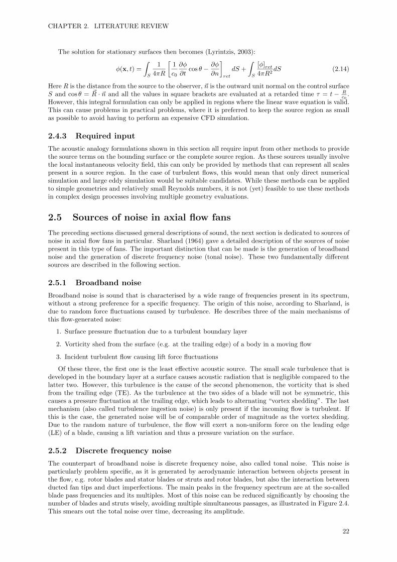
The first validation for the DSNG method is the test case of an airfoil and slat, in the configurationas shown in Figure 3.1. The sound pressure levels are measured at various angles at the pressure andsuction side. The angles are measured counter clock-wise with respect to the center of the camber line,being zero degrees at the trailing edge. The results of these measurements are shown in Figure 3.2.
The results show good agreement in the prediction of broadband noise for high frequencies. Forfrequencies below 1000 Hz, the DSNG method overpredicts the experimental values significantly.
Figure 3.1: Airfoil and slat test case configuration. The image shows the CFD mesh with the turbulentkinetic energy. The region enclosed by the red square is used as source region for the DSNG method.(From: di Francescantonio et al. (2013))
29

CHAPTER 3. BENCHMARKS & OUTLINE
Figure 3.2: Comparison of DSNG results and measurements for Airfoil and Slat configuration at differentangles. (From: di Francescantonio et al. (2013))
30

CHAPTER 3. BENCHMARKS & OUTLINE
θ
Figure 3.3: Absolute Mach number distribution for the QinetiQ circular nozzle with a diameter of 86mm.Sound pressure levels are measured for the angle θ between 30 and 110 degrees at a distance of 1.8mfrom the center of the nozzle exit. (Adapted from: NUMECA (2014a))
3.1.2 3D Nozzle
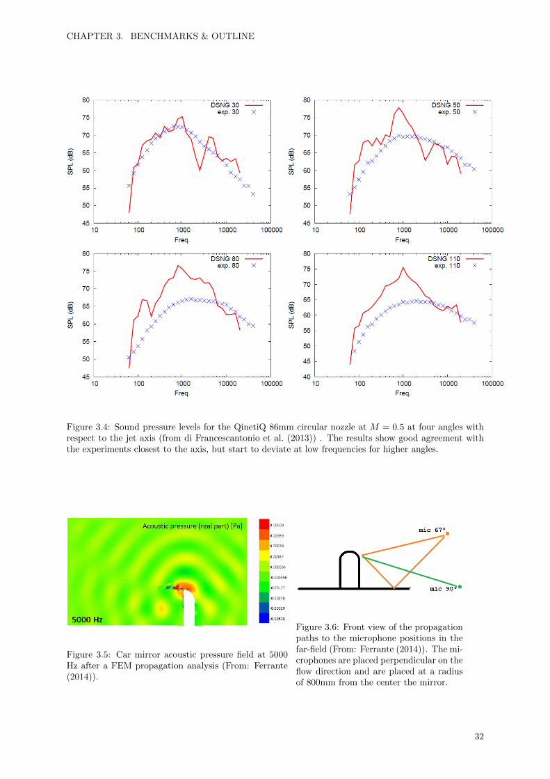
The second test case is a QinetiQ circular nozzle of 86mm at a speed of M = 0.5. A three-dimensionalRANS analysis using the shear stress transport model was performed. The resulting absolute Machnumber distribution is shown in Figure 3.3. Also the angle θ that is varied for the sound pressure levelmeasurements is displayed. The results are shown in Figure 3.4. The results show very good agreementover the complete frequency range for the measurements close to the axis. The results at increasing anglesdecrease in accuracy, this is most likely due to the propagation analysis conducted after the turbulentsources where reconstructed. This propagation was conducted assuming a steady medium, so the effectsof non uniformities in the flow have been neglected. These results might be improved by embedding thecomputed sources as volume sources in a finite element frequency domain solver for non uniform flows.
3.1.3 Car mirror
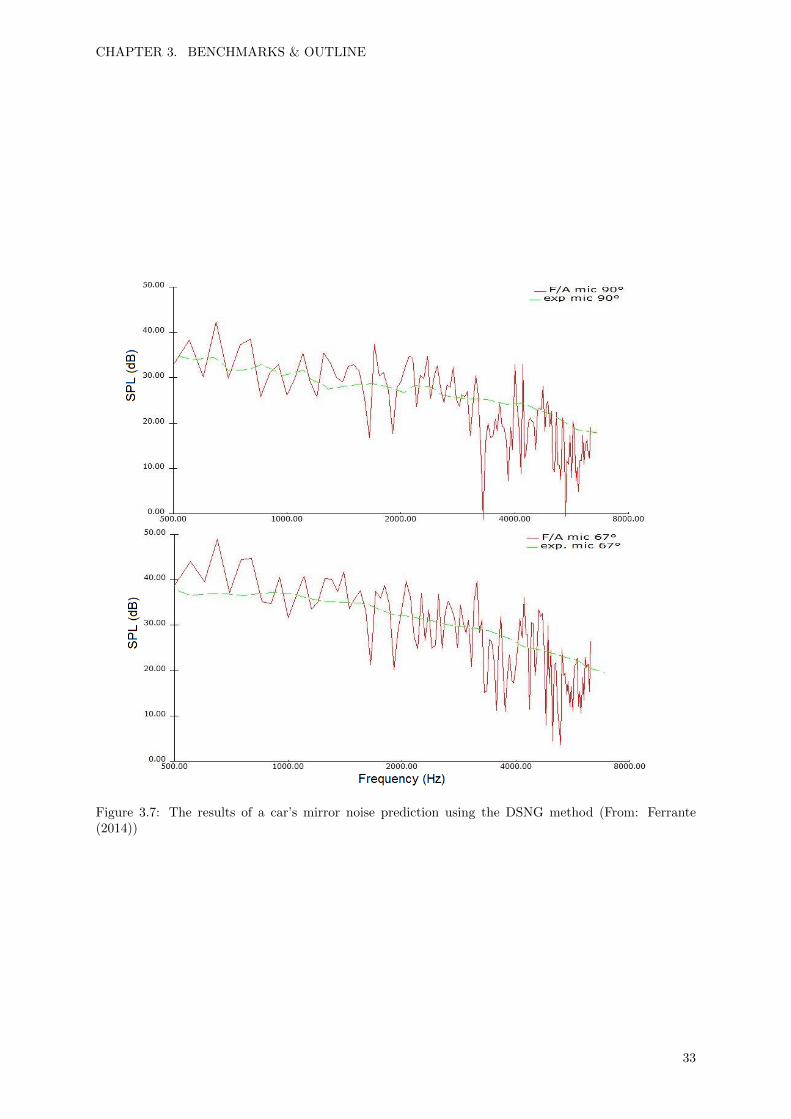
The last test case that is presented for the DSNG method is the analysis of the noise emitted by a flowaround a car mirror. This analysis was described by Ferrante (2014). The analysis covers the creationof a CFD mesh, a CFD steady RANS analysis, the generation of a mesh for stochastic reconstruction,the evaluation of the acoustic sources and an acoustic FEM propagation analysis. The resulting acousticpressure field for 5000 Hz after the FEM propagation is shown in Figure 3.5. From the boundaries of theFEM domain, a far-field radiation analysis is performed to predict the sound pressure level at the twofar-field microphones shown in Figure 3.6. The results are shown in Figure 3.7. The agreement betweenthe experiments in this case is good for the complete spectrum.
3.2 Outline
The cases described above show the applicability of the DSNG method to two- and three-dimensionalproblems. All the examples described consider non-rotating equipment. The method shows potentialas a prediction method for engineering purposes, but the method has not yet been applied to rotatingequipment in general and low-speed axial fans specifically.
The validation of this method for low-speed axial fans is the objective of the remainder of this thesis.To apply and validate this method, a complete set of experimental results has been very kindly providedby Howden Netherlands. A complete set of required software packages, has been very kindly provided byNUMECA. This forms a solid basis for the validation of the DSNG technique, being able to perform allthe steps necessary with the provided software and to make a comparison with the experimental resultsto assess the quality of the prediction method.
The steps that should be performed in the prediction process are roughly the same as with the car’smirror analysis. However, in the far-field radiation analysis, the transition between a rotating and a
31
CHAPTER 3. BENCHMARKS & OUTLINE
Figure 3.4: Sound pressure levels for the QinetiQ 86mm circular nozzle at M = 0.5 at four angles withrespect to the jet axis (from di Francescantonio et al. (2013)) . The results show good agreement withthe experiments closest to the axis, but start to deviate at low frequencies for higher angles.
Figure 3.5: Car mirror acoustic pressure field at 5000Hz after a FEM propagation analysis (From: Ferrante(2014)).
Figure 3.6: Front view of the propagationpaths to the microphone positions in thefar-field (From: Ferrante (2014)). The mi-crophones are placed perpendicular on theflow direction and are placed at a radiusof 800mm from the center the mirror.
32
CHAPTER 3. BENCHMARKS & OUTLINE
Figure 3.7: The results of a car’s mirror noise prediction using the DSNG method (From: Ferrante(2014))
33

CHAPTER 3. BENCHMARKS & OUTLINE
Define geometry
AutoBlade
GenerateCFD grid
AutoGrid
Set-up & performCFD Simulation
FINE/Turbo
Generatemeshforstochasticreconstruction
FINE/Acoustics
FlowNoise sourcereconstruction
FINE/Acoustics
Acoustic propagationin duct using FEM
FINE/Acoustics
Far-Field radiaton
FINE/Acoustics
Generate acousticFEM meshHexpress/Hybrid
CFDpost-processing
CFView
Figure 3.8: Work flow diagram for a complete analysis of the flow noise evaluation at a far-field micro-phone. In the bottom right of each step, the program used to perform this action is displayed.
fixed domain is performed. A work flow diagram of the complete process is shown in Figure 3.8. Thisdiagram shows the steps needed to obtain a sound pressure level (SPL) at a far-field microphone.
The prediction of the aerodynamic performance is done using the program FINE/Turbo, this programcan be used in various CFD calculation, but is especially tailored for the prediction of the performance ofturbomachinery. The theory applied in this program and the prediction of the aerodynamic performanceby this program are described in chapter 4 and chapter 5, respectively. The DSNG method with thepossibility to take into account rotational effects, is incorporated in an alpha-release of the programFINE/Acoustics. All the steps performed within this program and the results of the acoustic analysisare described in chapter 6. Finally, the conclusions and recommendations are presented in chapter 7.
34

Chapter 4
Numerical flow reconstruction
This chapter describes the steps that have to be taken to reconstruct the flow field of a fan usingcomputational fluid dynamics (CFD). The steps reported here are universal for most commercial CFDpackages, but the examples apply to the NUMECA CFD package FINE/Turbo. Firstly, the governingset of equations is formulated, then the time-averaging of this equations using Favre- and Reynoldsaveraging is described. This averaging leads to a ’closure problem’, which necessitates the introductionof turbulence models, introducing additional equations to be able to close the system. Once the set ofequations describing the flow is formulated, the discretisation is described and two techniques to enhancethe convergence rate are elaborated. Finally, the convergence itself and the important factors in gridgeneration are treated.
4.1 Governing equations
The governing equations for the flow field are the compressible Navier-Stokes equations. This is a setof 5 equations, one representing mass conservation, three representing momentum conservation and onerepresenting energy conservation. The fluid is assumed to be a continuum and the fluid is of a fixedcomposition, not changing phase or changing its properties otherwise (e.g. chemical reaction). Theflow is does not have many restrictions, it can be unsteady, viscous, compressible and heat conducting.External force fields and heat sources can also be present. In the partial differential equation (PDE)conservation form presented here, the only restriction of the flow field is that the flow field variablesshould be continuous, that means no shocks should be present in the flow. For the analysis of low-speedaxial fans, this should not form any difficulty, as the flow is usually in a low Mach number regime. Thecomplete equations are shown symbolically in Equation 4.1:
∂
∂t~U + ~∇ · ~F = ~Q (4.1)
The vectors in the equations are, respectively, the 5 x 1 conservative variables vector ~U (Equation 4.2),
where E = e+ |~v|22 represents the total energy per unit volume with e the internal energy; the 5 x 3 flux
vector ~F (Equation 4.3), where τ is the stress tensor, H = E + pρ represents the specific total enthalpy
and the heat flux is defined by Fourier’s law, with κ the thermal conductivity and ~∇T the temperaturegradient. Evaluation of the divergence of the tensors within the divergence operator is performed forevery row of the tensor. The 5 x 1 vector ~Q contains the source terms (Equation 4.4), where ~fe are
the external forces, Wf = ρ~fe · ~v is the work performed by these external forces and q represents thevolumetric heat sources. The effects of gravity are neglected in this analysis, as it is of minor influencein axial fans.
~U =
ρρ~vρE
(4.2)
~F =
ρ~vρ~v ⊗ ~v + pI − τ
ρ~vH − τ · ~v − κ~∇T
(4.3)
35
CHAPTER 4. NUMERICAL FLOW RECONSTRUCTION
~Q =
0
ρ~feWf + q
(4.4)
If the flow considered is composed of a Newtonian fluid, the deviatoric stress tensor is given by:
τij = µ
[∂vj∂xi
+∂vi∂xj− 2
3
∂vk∂xk
δij
]for i, j = 1, 2, 3 (4.5)
Here µ is the dynamic molecular viscosity and δij is the Kronecker delta. The set of five equationscontains seven unknowns, three velocity components and four thermodynamic quantities: the density,pressure, temperature and the internal energy. To complete the formulation of the mathematical model,two equations of state are introduced. These equations are based on the thermodynamic state principle,which states that state of a fluid is fully determined by two independent thermodynamic quantities.With the assumption of a perfect gas, which according to Kundu et al. (2012) is valid for most gases(including air) at ordinary temperatures and pressures, these equations can be formulated as:
p = ρRT (4.6)
e = cvT (4.7)
With R the specific gas constant, which is 287 J/kgK for air and cv is the specific heat at constantvolume.
4.2 Reynolds Averaged Navier-Stokes equations
The aim of this research is, as described in chapter 3, to investigate whether the noise of a fan can bepredicted for engineering purposes. This means that computational time is an important limiting factor.Equation 4.1 covers all length and time scales, from the main flow features to the smallest vortices.This will require a very fine computational grid, to represent all scales present in the flow. Thus,the computational effort needed for solving this set of equations directly is not feasible for engineeringapplications. To reduce the computational time, the turbulent flow can be approximated. The mostwidely applied method in industry is the Reynolds Averaged Navier-Stokes (RANS) model, this model isbased on the decomposition of the local, time-dependent flow properties in the sum of a time-independentmean value and a fluctuating part, this time averaging can be defined for any variable Ψ as:
Ψ ≡ 1
T
∫T
Ψ(t)dt, Ψ′ ≡ Ψ−Ψ (4.8)
In the case of a compressible flow, the most convenient way of averaging these equations is by using theFavre-average, this is a density-weighted average, which has the advantage of removing products of thefluctuations with other fluctuating quantities that arise in the averaging process. The Favre-average isdefined as:
Ψ =ρΨ
ρ, Ψ′′ ≡ Ψ− Ψ (4.9)
Note that in general Ψ′ is equal to zero and Ψ′′ is unequal to zero, but ρΨ′′ is equal to zero. When forinstance applying these averages to the first equation of Equation 4.1, the mass conservation equation,the velocity is decomposed into its Favre-average and its corresponding fluctuation and the completeequation is Reynolds averaged:
∂ρ
∂t+ ~∇ ·
(ρ~v + ρ~v′′
)= 0 (4.10)
Assuming that the flow field is differentiable in both time and space, the averaging operator and differ-entiations are interchangeable. This results in the final averaged mass conservation equation:
∂ρ
∂t+ ~∇ ·
(ρ~v)
+ ~∇ ·(ρ~v′′)
=∂ρ
∂t+ ~∇ ·
(ρ~v)
= 0 (4.11)
In a similar way, this technique can also be applied to the momentum equations. In the absence of bodyforces, this results in (Hirsch, 2007):
∂ρ~v
∂t+ ~∇ ·
(ρ~v ⊗ ~v + pI − τV − τR
)= ρ~fe (4.12)
36

CHAPTER 4. NUMERICAL FLOW RECONSTRUCTION
Here τV contains the averaged viscous shear stresses, and τR represent the Reynolds stresses. ThisReynolds stress term is a non-linear term, defined by
τR = −ρ~v′′ ⊗ ~v′′ (4.13)
This term forms the major challenge, as the relation between these Reynolds stresses and the mean floware generally not known. This is what is known as the ’closure problem’ in turbulence, this is elaboratedin the following section.
To complete this set of averaged equations the energy equation is also averaged using a combinationof Reynolds- and Favre-averaging, this results in (NUMECA, 2014c):
∂
∂t
(ρE)
+ ~∇ ·[(ρE + p
)~v + ρE′′~v′′ + p~v′′ − (κ+ κt)~∇T − τ · ~v
]= Wf + q (4.14)
Here E = e + 12 ~v · ~v + k and κt is the turbulent thermal conductivity. This parameter is connected to
the turbulent eddy viscosity µt as:
κt =µtcpPrt
(4.15)
Here Prt is the turbulent Prandtl number (≈ 1 for air) and cp is the heat capacity at constant pressure.
The parameters k and µt are described in detail in the following section.
4.3 Model closure – Turbulence modelling
To be able to close the model, the Reynold stresses expressed in Equation 4.13 can be modelled using theturbulent viscosity hypothesis of Boussinesq (Schmitt, 2007). To do this, first the notation is switchedto index notation, with this Equation 4.13 can be rewritten as:
− ρv′′i v′′j = −ρ
(ρv′′i v
′′j
ρ
)= −ρv′′i v′′j (4.16)
The trace of this tensor is proportional to the Favre-averaged turbulent kinetic energy (using the Einsteinsummation convention):
k =1
2(ρv′′i v
′′i /ρ) =
1
2v′′i v′′i (4.17)
Note that here the lower case letter k instead of the capital K now denotes the turbulent kinetic energyand not the wavenumber. Using this notation, the turbulent viscosity hypothesis can be formulated as:
− ρv′′i v′′j = µt
[∂vi∂xj
+∂vj∂xi− 2
3
∂vk∂xk
δij
]− 2
3ρkδij for i, j = 1, 2, 3 (4.18)
Here δij is the Kronecker delta and µt represents the turbulent eddy viscosity. It is this eddy viscosity,that forms the basis for the group of eddy viscosity turbulence models (Pope, 2000). There are manymodels which try to represent the real turbulent flow features as much as possible, but the use ofempirically determined parameters is inevitable. The model should maintain as much information aboutthe flow field as possible, but without introducing a lot of extra computational time. The models thatare most widely used in and adapted to the turbomachinery industry, and are also applied in this thesis,are the Spalart-Allmaras (SA) 1-equation model and the shear stress transport (SST) 2-equation model.As the Spalart-Allmaras model contains only one additional equation, it does not require a lot of extracomputational time. The SST model contains two additional equations, but its major advantage in thiscase is that it also gives additional information about the flow field, in particular the turbulent kineticenergy and the turbulence dissipation rate. These latter two variables form the input for the acousticalanalysis described in chapter 6.
4.3.1 Spalart-Allmaras model
The Spalart-Allmaras model is a one-equation model, introduced by Spalart and Allmaras (1994), es-pecially developed for aerodynamic applications. They realised that the one-equation models present atthe time did not perform well, especially the implementation of the models for flows around complexstructures was hard. This was due to the fact that the models treated the boundary layer as a single,
37

CHAPTER 4. NUMERICAL FLOW RECONSTRUCTION
tightly coupled module, i.e. they are non-local models. This caused a severe lack of accuracy in separat-ing flow or shear layers. With the introduction of the Spalart-Allmaras model, which applies a semi-localmethod with limited influence of the surrounding flow field, flow separation can be predicted.
In the Spalart-Allmaras model, the turbulent eddy viscosity is computed from:
µt = ρνfν1 (4.19)
Here ν is the turbulence variable that is solved from a transport equation, shown in Equation 4.21 andfν1 is defined by:
fν1 =χ3
χ3 + c3ν1
, where χ =ν
ν(4.20)
Here ν is the molecular kinematic viscosity. The transport equation for ν that is solved is given by:
Dν
Dt=
1
σ∇ · [(ν + (1 + cb2)ν)∇ν]− cb2ν∆ν+ ST (4.21)
Here the left hand side represents the advection along a streamline and on the right hand side, cb2 andσ are constants and ST represents the sources, defined as:
ST = cb1Sν − cw1fw
(ν
d
)2
, (4.22)
which is further defined with:
fw = g
(1 + c6w3
g6 + c6w3
) 16
; S = Sfν3 +ν
κ2d2fν2; (4.23)
fν2 =1
(1 + χ/cν2)3; fν3 =
(1 + χfν1)(1− fν2)
χ, (4.24)
in these equations cw3 and κ are model constants, d is the distance to the nearest wall, S is the magnitudeof the vorticity and g is defined as:
g = r + cw2(r6 − r), where r =ν
Sκ2d2(4.25)
The constants arising in the model are:cw1 = cb1/κ
2 + (1 + cb2)/σ, cw2 = 0.3, cw3 = 2, cν1 = 7.1, cν2 = 5cb1 = 0.1355, cb2 = 0.622, κ = 0.41, σ = 2/3
To be able to apply the Spalart-Allmaras, additional boundary and initial conditions have to beapplied. On solid walls with the no slip condition (i.e. ~v− ~vwall = 0), the turbulent eddy viscosity is setto zero. For the inlet boundary it is recommended to set the kinematic turbulent viscosity by settingthe ratio of νt/ν between 1 and 5, this ratio is dependent on the actual level of turbulence present in themean flow. The initial solution throughout the domain can be best set to νt/ν ≈ 2 · 10−7ReC , accordingto Spalart and Rumsey (2007), where ReC is the Reynolds number based on the chord length. For moredetails on the model implemented in FINE/Turbo, see Ashford (1996).
4.3.2 Shear stress transport model
To resolve the turbulent viscosity with improved accuracy, two equation models are often implementedin commercial CFD packages. Usually they resolve the turbulent viscosity by solving two transportequations, one for the turbulent kinetic energy (k) and one for the turbulence dissipation rate (ε) or theturbulence frequency (ω). The Favre-averaged turbulent kinetic energy (k) is defined in Equation 4.17.The dissipation rate, with τij the deviatoric stress tensor defined in Equation 4.5, is defined as:
ε ≡ 1
ρτij∂v′′i∂xj
(4.26)
The turbulence frequency is defined as:
ω ≡ ε
k(4.27)
38

CHAPTER 4. NUMERICAL FLOW RECONSTRUCTION
The shear stress transport (SST) model is a combination of multiple models, combining the strengths ofthe k − ε turbulence model developed by Jones and Launder (1972) and the k − ω model described indetail by Wilcox (1993). The k− ε model is the most used and simplest two-equation model, but it doesnot perform well in near-wall regions. The k−ω model on the other hand, does perform well in treatmentof the viscous near-wall region, but is very sensitive to turbulence boundary conditions specified at freestream boundaries (Pope, 2000). Menter (1994) proposed the combination of both of these models, byusing the k − ω model as basis, but using a blending function in the equation for ω, where at the solidboundaries it represents the standard k−ω model and transitions to the k− ε model further away fromthe wall. In this model the turbulent viscosity is determined from:
νt =a1k
max(a1ω,√
2SF2)(4.28)
where a1 is a constant, S is the magnitude of the vorticity, introduced to improve the prediction for flowswith adverse pressure gradients and F2 is a blending function, depending on the distance to the nearestwall (d), given by:
F2 = tanh
[
max
(2√k
β∗ωd,
500ν
ωd2
)]2 (4.29)
The transport equations for k and ω that are solved are given by (NUMECA, 2014c):
Dk
Dt= Pk − β∗ωk +
∂
∂xj
((ν + σkνt)
∂k
∂xj
)(4.30)
Dω
Dt= γ
ω
kPk − βω2 +
∂
∂xj
((ν + σωνt)
∂ω
∂xj
)+ 2(1− F1)σω2
1
ω
∂k
∂xj
∂ω
∂xj(4.31)
Here Pk is the production rate of turbulence and β∗ is a constant. The variables γ, β, σk and σω areall defined by blending the coefficients of the original k − ω (subscript 1) and the transformed k − ε(subscript 2) models using the following equation, where φ denotes any of these variables:
φ = F1φ1 − (1− F1)φ2 (4.32)
The blending function F1 is given by:
F1 = tanh
min
[max
( √k
β∗ωd,
500ν
ωd2
),
4ρσω2k
CDkωd2
]4 , (4.33)
with CDkω = max(
2ρσω21ω∂k∂xj
∂ω∂xj
, 10−20)
.
The model constants are defined as:γ1 = 0.5532, β1 = 0.075, σk1 = 0.85, σω1 = 0.5γ2 = 0.4403, β2 = 0.0828, σk2 = 1, σω2 = 0.856a1 = 0.31, β∗ = 0.09
To be able to apply the SST model, additional boundary and initial conditions have to set, thesevalues based physical arguments and experience. On the solid walls where the no-slip condition is applied,all velocity fluctuations vanish on this wall. This means the that the turbulent kinetic energy k will bezero. The initial and boundary condition for k can be determined using the turbulence intensity I. Thisparameter relates the stream wise reference velocity (e.g. the inlet velocity) to the fluctuating velocity:
I =v′′rms
Uref(4.34)
Assuming that the turbulence is isotropic, the turbulent fluctuations can be written as:
k =3
2(v′′rms)
2(4.35)
For internal flows, this turbulence intensity is around 5% Using this value and Equation 4.34 and4.35, an estimate for the value of k can be made.
39

CHAPTER 4. NUMERICAL FLOW RECONSTRUCTION
The turbulent dissipation can be estimated using (NUMECA, 2014c):
ε =c3/4µ k3/2
l(4.36)
Here l is typically 0.07DH , with DH being the hydraulic diameter and cµ = 0.09 is a model constant.
4.4 Discretisation
Now that the set of equations describing the flow (4.1-4.4) is formulated and the set of equations isclosed, the equations are expressed in conservation form as:
∂
∂t
∫∫∫Ω
~UdΩ +
∫∫S
~F · d~S =
∫∫∫Ω
~QdΩ, (4.37)
where Ω is the control volume and S is its bounding surface. To solve this equation, the flux vector ~Fis first split in a viscous and inviscid part:
~F = ~F I − ~FV =
ρ~v
ρ~v ⊗ ~v + pI − τR(ρE + p
)~v + ρE′′~v′′ + p~v′′
− 0
τV
(κ+ κt)~∇T + τ · ~v
(4.38)
The spatial discretisation is based on a cell centered control volume approach. Therefore, for everyarbitrary control volume ΩJ , the integral conservation law of Equation 4.37 can be replaced by itsdiscrete form, where the volume integrals are averaged over the cell and the surface integral can bereplaced by the sum over all the bounding faces:
∂
∂t
(~UJΩJ
)+∑faces
~F I ·∆~S −∑faces
~FV ·∆~S = ~QJΩJ (4.39)
To solve this semi-discrete equation, the viscous flux term is determined by a standard central discreti-sation scheme. The inviscid flux term is determined by a central discretisation scheme with an artificialdissipation term, as described by Jameson et al. (1981). This scheme can be applied in combinationwith a time discretisation. In low Mach number regimes, time-marching algorithms that are appliedto compressible flow show a lack of efficiency. When for instance Equation 4.39 is solved for a domainwhere the flow velocities become small compared to the speed of sound, the solution will converge slowly.Multiple methods exist to speed up convergence, of which two are elaborated here.
4.4.1 Local time stepping
For every explicit scheme, the discretisation should satisfy the CFL condition, which is a limitation on theratio between the time and length scale (Equation 4.40). In steady state analyses, such as the modellingof a single flow channel in turbomachinery, the time derivatives that appear in the equations have nophysical meaning. Thus, this time derivative can be used in solving for the steady state as quickly aspossible. By adapting this time step locally, the computational effort can be reduced significantly.
CFL = ∆tvi
∆xi≤ CFLmax (4.40)
4.4.2 Preconditioning
The second enhancement that can be applied to the set of equations is preconditioning. As the timederivative does not have a physical meaning, it can be adjusted to reach the steady state solution faster.In this thesis Hakimi preconditioning is applied (Hakimi, 1997). The original time dependent part ofthe equations is multiplied by a preconditioning matrix Γ(Uref , β
∗), a function of a reference velocityand a preconditioning parameter β∗. The aim of this preconditioning is to reduce the ’stiffness’ ofthe eigenvalues of the system, which usually leads to numerical instability, unless step sizes are verysmall. The reduction of the stiffness results in a system that is easier to solve. The disadvantage of thispreconditioning is the possibility of adding too much artificial dissipation if the preconditioning is notperformed properly.
40

CHAPTER 4. NUMERICAL FLOW RECONSTRUCTION
4.5 Convergence criteria
The final set of equations is solved by an iterative solver using a multigrid approach. To see if a correctsteady state solution is reached, multiple checks can be performed. The first one is monitoring the RMSresidual. The residuals are calculated in each cell of the grid (Res =
∑R(U)) and scaled with the cell
volume:
RMSRes = log
(RMS(
Res
Vcell)
)(4.41)
This RMS residual is normalised using the RMS residual after the first iteration. In general, for engi-neering purposes a residual reduction of 4 orders of magnitude is considered as a suitable convergence,but it highly depends on the initial solution. Therefore, stabilisation of the residual is also an importantfactor. If the residual has been reduced and stabilised to an acceptable level, for every CFD analysisthe solution that is found for a specific grid should not change significantly when using another grid. Toensure this, a grid refinement study should be performed. In this thesis this is performed in section 5.6.
4.6 Near wall mesh quality
To ensure that the chosen turbulence models are applicable, especially the mesh near the wall should becreated with care. Certain criteria have to be satisfied to properly capture all the high gradients presentin this region where viscous effects play an important role.
To capture these viscous effects properly, two approaches can be used. The first is to use a wall-function, this is based on the existence of a ‘log-layer’ first described by Von Karman (1930). He foundthat the average velocity of a turbulent flow near a wall, is at some distance from the wall related to thelogarithm of that distance. This is what is now known as the ‘law of the wall’. The second approachis to resolve the complete boundary layer by making sure that the boundary layer contains a sufficientnumber of grid points.
In general a turbulent boundary layer exists of a viscous sublayer, a buffer layer and the log-lawregion described by Von Karman (Pope, 2000). The wall-function approach applies boundary conditionsbased on the log-law relations at some distance away from the wall. This way the turbulence modelequations do not have to be solved close to the wall. This theory however, is not applicable when effectsof flow separation are of importance. When separation occurs, the boundary layer in this detaches fromthe surface and flow starts to recirculate after this point. This can not be properly modelled by thewall-function approach. For the analysis performed in this thesis, regions of separated flow might occur.Therefore, wall-functions are not applied.
To capture all effects present in the flow near solid boundaries, the boundary layer should containa sufficient number of grid points. The most important parameter in creating the grid in this region isthe cell width of the first cell at the wall, denoted as ywall. To estimate this ywall, the 1/7th power lawvelocity profile is assumed. In this way the skin friction coefficient is related to the Reynolds number as(NUMECA, 2014c):
Cf =0.027
Re1/7x
(4.42)
Using this friction coefficient and a reference velocity, the friction velocity (uτ ) can be estimated (Equa-tion 4.43) and with this result and a given y+ value, the maximum inner cell width can be estimatedusing Equation 4.44:
uτ =
√τwallρ
=
√1
2V 2
refCf (4.43)
ywall =νy+
uτ(4.44)
To be able to take into account all effects in the flow, the first cell should be placed in the viscoussublayer. The viscous sublayer usually extends to y+ ≈ 5 (Pope, 2000), therefore the desired y+ value isset to 1.
In the fan considered in this research, the chord is taken as the reference length(C = 0.347 m), anapproximation of the average axial velocity as the reference velocity (Vref = 10 m/s) and the kinematicviscosity to be ν = 1.5 · 10−5 m2/s. With these values, the maximum width of the first cell becomesywall = 3.1 · 10−5 m. To ensure that the solution obtained on a specific grid, the true y+ value shouldbe checked after an analysis. This value could be deviating from the set value, because it is dependenton locally solved variables and Equation 4.44 is estimated based on a global reference velocity.
41

CHAPTER 4. NUMERICAL FLOW RECONSTRUCTION
42

Chapter 5
Prediction of aerodynamicperformance
In this chapter the theory described in chapter 4 is applied to a low-speed axial fan. The analysesare performed in the commercial CFD suite FINE/Turbo, and the post-processing is performed usingCFView, both kindly provided by NUMECA. Firstly, an overview of the modelled geometry and thecomputational domain are given. Then the results for the CFD analyses are checked for proper conver-gence. Also, an estimate is made of the discretisation error with a grid refinement study. Finally, thecomputational results are compared with the experimental results, such as efficiency, shaft power andpressure rise, obtained at the Howden test facility. When good agreement is found between experimentsand CFD, these CFD results form adequate input for the acoustical analysis.
5.1 Difficulties encountered
The prediction of the aerodynamic performance is not a straightforward task, many factors are of influ-ence in the process that could influence the end result. At first a lot of effort was invested in the CFDanalysis, but the results seemed to underestimate the pressure rise of the fan significantly. To try andexplain this difference many changes to the CFD model were made, such as a significant change in bladeangle, changing the duct length and changing inlet boundary conditions. However, all these changes didnot lead to significant improvement in the prediction with respect to the experimental results. This led tosignificant doubt in the experimental results, therefore a set of experiments was repeated. Unexpectedresults were obtained, as the new experimental values were significantly deviating from the previousresults. Repeating these experiments was a necessity in the current analysis, but thanks to these ex-periments, very valuable practical experience has also been gained. The rerun of the experiments gavevaluable insight in the experimental process and measurements performed. The difference between thetwo sets of experiments is shown in Appendix A.2.
The results presented in this chapter are therefore the outcome of a long process, where many im-provements have been made in both the CFD and the experimental results.
5.2 Geometry
The geometry of the computational domain is created with as much similarity to reality as possible,but simplifying enough to keep computational time within reasonable limits. The complete experi-mental set-up and test methods are described in Appendix A. The major differences between theexperimental and computational analyses are elaborated in the following sections. A global lay-out ofthe experimental set-up is shown in Figure 5.1, where the numbers indicate the following components(from: Howden Netherlands b.v. (2014)):
1. Tunable inlet valve
2. Booster fan
3. Outlet guide vanes
43

CHAPTER 5. PREDICTION OF AERODYNAMIC PERFORMANCE
Figure 5.1: Experimental set-up, the dotted line box at the right shows the computational domain(From: Howden Netherlands b.v. (2014)).
4. Settling screens
5. Nozzle
6. Electric motor
7. Settling screens
8. Test fan
The nozzle is used to determine the flow rate through the system. The inlet valve and booster fan areused to be able to test the complete operating range of a fan. When testing at high flow rates, theresistance of the system (from #3 to #7) will become too large for the test fan to overcome. Therefore,the booster fan (#2) is activated to be able to help overcome part of the system resistance at high flowrates. For low flow rates, the booster fan is turned off and the tunable inlet valve can be closed to increasethe resistance, up to the point where the flow rate becomes zero. Modelling this complete system is notfeasible nor necessary, as measurements of the flow conditions that could be affected by the system areperformed after the last settling screens (#7). The section highlighted by the dotted line box aroundthe test fan is the part that is simulated in the CFD analysis.
The second reduction of the model is in the periodicity. The flow is considered as steady in therotating frame of reference, this means that only a single flow channel needs to be modelled. In thiscase, the machine contains three rotor blades, so one third of the full machine is modelled, containingone blade. The full computational domain is shown in Figure 5.2.
The rotation is defined positive as defined in the direction indicated, the impeller rotates in the oppo-site direction (i.e. counterclockwise seen from the inlet). The radius of the hub (rh) is set correspondingto the start of the blade at 0.1925m. The radius of the tip (rt) is set at 0.9144m (3 ft). The length ofthe inlet and outlet are set according to the dimensions of the experimental fan duct being Lin = 0.57 mand Lout = 1.3 m. An overview of the dimensions and typical operating conditions is listed in Table 5.1.
5.2.1 Hub
An additional simplification is made in the modelling of the hub. In reality the hub is a disc withattached shaft that extends to the inlet. In the NUMECA AutoGrid5 meshing program, the geometryis divided in meridional flow paths. For every flow path a blade to blade mesh is generated and finallya three-dimensional structured grid is created. If these meridional flow paths deviate strongly, a highquality structured grid cannot be constructed easily. Therefore, in the computational domain the hubis extended all the way through the domain, also to the outlet, to prevent difficulties in the meshing
44

CHAPTER 5. PREDICTION OF AERODYNAMIC PERFORMANCE
r z
θ
rh
rt
Lin
Lout
Figure 5.2: Computational Domain
Property ValueHub radius 0.1925 mTip radius 0.9144 m
Inlet length 0.57 mOutlet lenght 1.30 m
Blade chord length 0.347 mBlade pitch angle 15o
Rotational speed 495.35 RPMVolume flow (full machine) 16.9 m3/sFan static pressure (FSP) 151 Pa
Table 5.1: Computational domain dimensions and typical operating conditions (corresponding to theoperating point used for the acoustical analysis)
45

CHAPTER 5. PREDICTION OF AERODYNAMIC PERFORMANCE
procedure. As the velocities near the hub will be relatively small due to the low local blade velocity,it is assumed that the influence of the blockage of the flow by the hub will be negligible and thus thismodelling simplification is justified.
5.2.2 Tip clearance
In this model, the tip clearance effects are not taken into account. The model does not contain anyspace between the blade and the shroud. In reality, the tip gap was measured to be approximately 5mm. This is 2.7% of the fan diameter. Personal communication with a previous graduate student whoperformed detailed work on the influence of the tip gap in axial fans showed that the losses introducedwith such a gap are in the range between 5 and 10 percent. As the region of the tip gap shows significantsecondary flow phenomena, it demands a very fine computational grid and thus introduces a lot of extracomputational effort. Therefore it is neglected in the current analysis, as the goal of this present analysisis to create a first input for the acoustic analysis.
5.2.3 Blade modelling with AutoBlade
The blade geometry is given by a range of 49 data points for the pressure and suction side, as the bladeis not swept or staggered, the profile is the same over the complete span. Using the AutoBlade moduleof NUMECA, the blade shape is fitted to the native NUMECA format. The result of this fitting processis shown in Figure 5.3. Only the leading edge of the blade shows a small discrepancy with respect tothe original geometry. This is caused by the larger than 90 degree angle between the camber line andpressure side, which the program is unable to describe in its native format.
Blade pitch angle
To define the blade pitch angle, a line is drawn from the trailing edge, which touches at the pressureside, as shown in Figure 5.3(a). When this line is perpendicular to the flow direction, the blade is, bydefinition, at a rotation of zero degrees. In all results presented here, the blade rotation is fifteen degrees.
5.3 Boundary conditions
Now that the geometry is fully defined, the appropriate boundary conditions have to be selected. To keepthe simulation as close to experiments as possible, the inlet and outlet boundary conditions for the CFDdomain are defined using data that is also measured in the experiment. The inlet boundary conditionis defined using velocity components, calculating the axial velocity from the measured volume flow andthe inlet area. Assuming that the incoming flow is uniform and directed axially, the axial velocity is theonly non-zero velocity component. The value for the static temperature is set at 293K at the inlet anddepending on the turbulence model selected, the turbulent viscosity (µt) or the turbulent kinetic energy(k) and the turbulence dissipation rate (ε) are set according to the equations defined in section 4.3. Atthe outlet the measured static pressure is set as a boundary condition, this means that the total pressureat the inlet will be the variable that finally determines the fan static pressure.
As the domain covers only one section of the machine, the interface with the neighbouring sectionsshould also be set. As the flow in each flow channel was assumed to be equal, the interfaces separatingthese channels are set to periodic. The blades, hub and shroud are all set to adiabatic solid boundarieswith the no-slip condition applied, i.e. the absolute velocity of the fluid at the wall is equal to the wallvelocity. The shroud is set to stationary and the hub and blades are set to the rotational speed measuredin the experiments.
5.4 Computational Grid
Once the computational domain is fully defined, the domain has to be discretised into a good qualitymesh. This is done using the AutoGrid5 program. A program that is designed to create structuredmeshes for turbomachinery. The meshing in this program is done in three major steps:
1. Generation of meridional flow paths.
2. Generation and control of 2D meshes on blade to blade surfaces
46
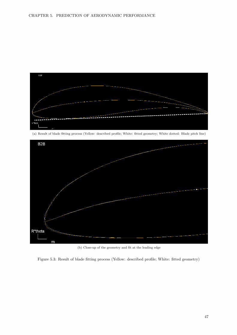
CHAPTER 5. PREDICTION OF AERODYNAMIC PERFORMANCE
(a) Result of blade fitting process (Yellow: described profile; White: fitted geometry; White dotted: Blade pitch line)
(b) Close-up of the geometry and fit at the leading edge
Figure 5.3: Result of blade fitting process (Yellow: described profile; White: fitted geometry)
47

CHAPTER 5. PREDICTION OF AERODYNAMIC PERFORMANCE
3. Generation of the 3D mesh, combining the meridional flow paths and 2D blade to blade meshes.
With these three steps, a mesh of hexahedral volumes is created by the program. In the first step, the wallcell width ywall is used as input, which is calculated using Equation 4.44. The program automaticallycreates multiple blocks, where the desired level of refinement can be set and the connectivity with otherblocks is ensured. To assess the quality of the mesh, the maximum aspect ratio, skewness angle andthe expansion ratio are monitored. A more detailed description of the meshing process is shown inAppendix B. The final mesh that is used for the Spalart-Allmaras calculations contains approximately2.0 million nodes. The grid used for the SST calculation contains approximately 3.3 million nodes.
5.5 Convergence of the results
To investigate if the solution is converged, several residuals are monitored in every analysis. The residualreduction graph for the SA simulation at the maximum efficiency point and the SST simulation aregiven in Figure 5.4. The residual stabilises just below 5 orders of magnitude reduction in the residualfor the SST simulation. The SA simulation was terminated because the residual dropped below the setconvergence criteria of 6 orders of magnitude reduction.
0 200 400 600 800 1,0001,2001,4001,600
−6
−4
−2
Iterations
Res
idu
al
SSTSA
Figure 5.4: The global residual calculated by FINE/Turbo for the SA simulation near the maximumtotal efficiency and for the SST simulation.
5.6 Numerical error estimation
The solution is obtained by an iterative solver on a discretised flow domain, using a multigrid approach.The discretisation of the equations means that there will always be a difference between the exact solutionand the discretised model, this is due to the truncation of higher order terms in the discrete approxima-tion. In theory however, when solving the system, the solution should converge when decreasing the gridsize. To see if this is the case, the grid is refined for the point where the maximum total efficiency is ex-pected. The refinement is applied systematically, refining the number of grid points in all directions withthe same factor. The results of this grid refinement study are processed using the procedure described inCelik et al. (2008). The discretisation error is estimated with the Grid Convergence Index (GCI), whichis based on Richardson extrapolation. As parameters for this error estimation, the fan static pressure,the total efficiency and shaft power are used, which are all denoted here as φ. The subscript of φ refersto the grid level, where 1 represents the finest grid. The three grids that are analysed are:
1. Finest grid: 11.2M grid points
2. Refined grid: 4.8M grid points
3. Original grid: 2.0M grid points
48

CHAPTER 5. PREDICTION OF AERODYNAMIC PERFORMANCE
The complete discretisation error analysis is described in more detail in Appendix D. The results ofthe discretisation error analysis are presented in Table 5.2. The maximum numerical uncertainty that isdetermined here is 2.8% for the fan static pressure. This is considered an acceptable level. Note that thisis solely the numerical error due to discretisation of the equations, so it does not account for modellingerrors.
φ = FSP [Pa] φ = ηtt[%] φ = Pshaft[W ]φ1 63.5 85.1 4817φ2 59.2 85.2 4737φ3 58.3 84.0 4717p 5.5 6.5 4.8φext21 64.7 85.0 4845CGI31 2.8% 0.29% 0.89%
Table 5.2: Discretisation error estimation results, grid 3 is used for the Spalart-Allmaras calculationsreported in the results
5.7 Aerodynamic performance
To assess the quality of the aerodynamic performance prediction by the CFD simulations, the CFDresults are compared to the measured experimental results using the dimensionless numbers elaboratedin chapter 1. The numbers compared here are the flow coefficient (Cf ), pressure coefficient (Cp), static(ηts) and total efficiency (ηtt) and the power coefficient (CP ). By using these parameters, the results caneasily be compared to other experiments. The complete procedure to obtain the experimental resultsis described in Appendix A. The complete list of settings used in the CFD computation is shownin Appendix C.
5.7.1 Results
The results of the CFD analyses are compared with the experimental results in Figure 5.5. The resultsof the Spalart-Allmaras (SA) model for the full curve are in good agreement with the experiments, thepressure coefficient has the same slope as the experimental curve for the usual operating range of the fan,but is slightly higher. The deviation of the pressure coefficient prediction is 11% at Cf = 0.15. At lowerflow coefficients, where the effects of stall become important, the agreement less satisfactory. The powercoefficient shows a larger deviation with the experiments, for low flow rates the curves still coincide, butat high flow rates the power required to drive the fan are overpredicted. The static efficiency trend ispredicted correctly for the higher flow rates and starts to deviate slightly from the experiments at valueslower than Cf = 0.15, similar to the pressure coefficient. The experimental quasi total efficiency showsgood qualitative agreement with the total efficiency computed by the simulations, both predicting thebest efficiency point at approximately the same flow coefficient. As expected, the absolute level is lowerfor the experiments due to only taking into account the average axial velocity.
Influence of turbulence model
To investigate the acoustical properties of the fan based on the theory described in subsection 2.7.1,several input parameters are required. In addition to the averaged velocities and density and pressureinformation, the turbulent kinetic energy (k) and the turbulent dissipation rate (ε) or turbulence fre-quency (ω) are required, this information is not provided by the CFD analysis using the Spalart-Allmarasturbulence model. Therefore, a single analysis using the shear stress transport (SST) model is performed,at a point on the fan-curve where sound pressure level measurements are available. For the acousticalanalysis it is preferred to use a simulation that was performed at the best efficiency point of the fan(Cf ≈ 0.2). However, in the measurements the booster fan (Figure 5.1 #2) is used to overcome the ex-cess pressure for experiments with a flow coefficient larger than 0.14. This means that no reliable soundmeasurements could be performed above this value of the flow coefficient. A reliable sound pressure levelmeasurement was obtained at a flow coefficient of 0.135. Therefore, the simulation with the SST modelwas performed at settings corresponding to this point on the fan-curve. The results of this analysis areshown in Figure 5.5 as well, also showing satisfactory agreement with the experimental values. The
49
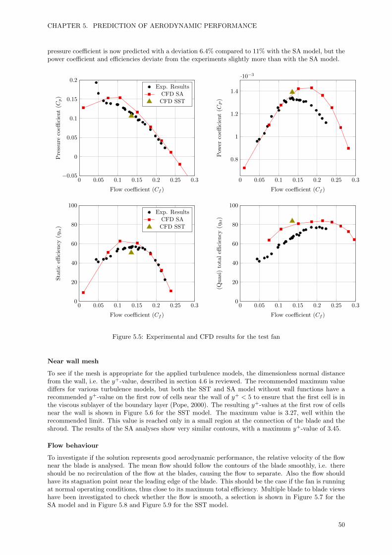
CHAPTER 5. PREDICTION OF AERODYNAMIC PERFORMANCE
pressure coefficient is now predicted with a deviation 6.4% compared to 11% with the SA model, but thepower coefficient and efficiencies deviate from the experiments slightly more than with the SA model.
0 0.05 0.1 0.15 0.2 0.25 0.3−0.05
0
0.05
0.1
0.15
0.2
Flow coefficient (Cf )
Pre
ssu
reco
effici
ent
(Cp)
Exp. ResultsCFD SACFD SST
0 0.05 0.1 0.15 0.2 0.25 0.3
0.8
1
1.2
1.4
·10−3
Flow coefficient (Cf )
Pow
erco
effici
ent
(CP
)
0 0.05 0.1 0.15 0.2 0.25 0.30
20
40
60
80
100
Flow coefficient (Cf )
Sta
tic
effici
ency
(ηts
)
Exp. ResultsCFD SACFD SST
0 0.05 0.1 0.15 0.2 0.25 0.30
20
40
60
80
100
Flow coefficient (Cf )
(Qu
asi)
tota
leffi
cien
cy(ηtt
)
Figure 5.5: Experimental and CFD results for the test fan
Near wall mesh
To see if the mesh is appropriate for the applied turbulence models, the dimensionless normal distancefrom the wall, i.e. the y+-value, described in section 4.6 is reviewed. The recommended maximum valuediffers for various turbulence models, but both the SST and SA model without wall functions have arecommended y+-value on the first row of cells near the wall of y+ < 5 to ensure that the first cell is inthe viscous sublayer of the boundary layer (Pope, 2000). The resulting y+-values at the first row of cellsnear the wall is shown in Figure 5.6 for the SST model. The maximum value is 3.27, well within therecommended limit. This value is reached only in a small region at the connection of the blade and theshroud. The results of the SA analyses show very similar contours, with a maximum y+-value of 3.45.
Flow behaviour
To investigate if the solution represents good aerodynamic performance, the relative velocity of the flownear the blade is analysed. The mean flow should follow the contours of the blade smoothly, i.e. thereshould be no recirculation of the flow at the blades, causing the flow to separate. Also the flow shouldhave its stagnation point near the leading edge of the blade. This should be the case if the fan is runningat normal operating conditions, thus close to its maximum total efficiency. Multiple blade to blade viewshave been investigated to check whether the flow is smooth, a selection is shown in Figure 5.7 for theSA model and in Figure 5.8 and Figure 5.9 for the SST model.
50
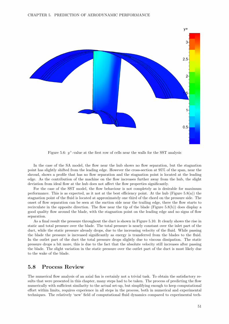
CHAPTER 5. PREDICTION OF AERODYNAMIC PERFORMANCE
Figure 5.6: y+-value at the first row of cells near the walls for the SST analysis
In the case of the SA model, the flow near the hub shows no flow separation, but the stagnationpoint has slightly shifted from the leading edge. However the cross-section at 95% of the span, near theshroud, shows a profile that has no flow separation and the stagnation point is located at the leadingedge. As the contribution of the machine on the flow increases further away from the hub, the slightdeviation from ideal flow at the hub does not affect the flow properties significantly.
For the case of the SST model, the flow behaviour is not completely as is desirable for maximumperformance. This is as expected, as it not at the best efficiency point. At the hub (Figure 5.8(a)) thestagnation point of the fluid is located at approximately one third of the chord on the pressure side. Theonset of flow separation can be seen at the suction side near the trailing edge, there the flow starts torecirculate in the opposite direction. The flow near the tip of the blade (Figure 5.8(b)) does display agood quality flow around the blade, with the stagnation point on the leading edge and no signs of flowseparation.
As a final result the pressure throughout the duct is shown in Figure 5.10. It clearly shows the rise instatic and total pressure over the blade. The total pressure is nearly constant over the inlet part of theduct, while the static pressure already drops, due to the increasing velocity of the fluid. While passingthe blade the pressure is increased significantly as energy is transferred from the blades to the fluid.In the outlet part of the duct the total pressure drops slightly due to viscous dissipation. The staticpressure drops a bit more, this is due to the fact that the absolute velocity still increases after passingthe blade. The slight variation in the static pressure over the outlet part of the duct is most likely dueto the wake of the blade.
5.8 Process Review
The numerical flow analysis of an axial fan is certainly not a trivial task. To obtain the satisfactory re-sults that were presented in this chapter, many steps had to be taken. The process of predicting the flownumerically with sufficient similarity to the actual set-up, but simplifying enough to keep computationaleffort within limits, requires experience in all steps in the process, both in numerical and experimentaltechniques. The relatively ‘new’ field of computational fluid dynamics compared to experimental tech-
51
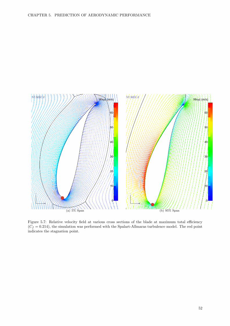
CHAPTER 5. PREDICTION OF AERODYNAMIC PERFORMANCE
(a) 5% Span (b) 95% Span
Figure 5.7: Relative velocity field at various cross sections of the blade at maximum total efficiency(Cf = 0.214), the simulation was performed with the Spalart-Allmaras turbulence model. The red pointindicates the stagnation point.
52

CHAPTER 5. PREDICTION OF AERODYNAMIC PERFORMANCE
(a) 5% Span (b) 95% Span
Figure 5.8: Relative velocity field at various cross sections of the blade at (Cf = 0.135) where soundmeasurement data is available, the simulation was performed with the SST turbulence model. The redpoint indicates the stagnation point.
53

CHAPTER 5. PREDICTION OF AERODYNAMIC PERFORMANCE
Figure 5.9: Close-up of Figure 5.8(a)of the relative velocity at the trailing edge. The onset of flowseparation is visible at the pressure side (top), while the standard boundary layer velocity profile isvisible at the suction side (bottom).
−0.5 0 0.5 1
9.92
9.93
9.94
9.95
9.96·104
Duct location(m)
Pre
ssu
re(Pa)
Static pressureTotal Pressure
Figure 5.10: Averaged pressure throughout the duct for the SST analysis. The vertical dotted linesindicate the position of the blade.
54

CHAPTER 5. PREDICTION OF AERODYNAMIC PERFORMANCE
niques makes it natural to perceive these numerical results with greater doubt. However, when a lot ofeffort is invested in obtaining numerical results similar to the experiments, one should also be wary ofthe quality of experimental results. The results presented in this chapter are the result of a completeprocess, reviewing every step thoroughly and checking the numerical and experimental results, but finallyforming a solid basis for further acoustical analysis.
55

CHAPTER 5. PREDICTION OF AERODYNAMIC PERFORMANCE
56

Chapter 6
Acoustics
This chapter covers the acoustical analysis of the low-speed axial fan whose aerodynamic performancehas been analysed in the previous chapter. This analysis is performed using an alpha-release (6.0.4) of theprogram FINE/Acoustics kindly provided by NUMECA. The program is presently still in a developmentphase, especially the application to rotating machinery is a recent addition to the program. All the stepstaken in this project are in the process of being streamlined into a single integrated analysis. This chapterdescribes all steps that are taken in the current version of the program, closely advised by NUMECA,to obtain a sound pressure level prediction (SPL) at a microphone, whose location corresponds to amicrophone location in the experimental measurements.
The first step that is performed is the creation of an adaptive mesh for the reconstruction of theturbulent flow field. This mesh is constructed based upon the averaged flow field variables obtainedfrom the RANS analysis. Secondly, this mesh is refined to be able to represent all frequencies that areof interest. After this, a FlowNoise analysis is performed and these sources are exported for use in thesubsequent finite element method analysis. This analysis solves the propagation of the sound inside thefan duct. Finally, the sound field on the outlet of the duct is propagated to a far-field microphone, takinginto account the rotational effects.
6.1 Turbulent field reconstruction
Using the theory described in section 2.7, as implemented in the FlowNoise module, the turbulent flowfield is reconstructed. To reconstruct this turbulent velocity field, a mesh is created depending on thelocal correlation length, that is extracted from the turbulent kinetic energy and dissipation computed bythe RANS analysis. For the SST turbulence model this local correlation length is computed by:
lRANS =2
3
k1/2
ω(6.1)
The meshing procedure can be summarised as (from: NUMECA (2014a)):
1. The source region is enclosed by a box region that is divided in 16x16x16 hexahedral elements;
2. For each hexahedron the minimum correlation length (lRANS) computed from the RANS analysis.If it is smaller than the hexahedron size, then the hexahedron is divided into 8 hexahedra. Thisstep is repeated recursively. When all the hexahedra are smaller than the local correlation length,the iterative process stops;
3. The CFD results are projected onto the hexahedral mesh. Nodes outside the original mesh are cutduring this process.
To check if this meshing is appropriate, a grid convergence study is performed, reconstructing the sourceregion on four different meshes. To do this, a grid refinement factor (r) is used in step 2 of the meshingprocedure. Using this refinement factor the hexahedron length is compared to a refined length lref =lRANS/r, instead of the standard correlation length obtained from the RANS analysis. The pressurefluctuations are probed at four different locations which contain a reasonable amount of turbulence, oneprobe is placed on the hub, one on the shroud and two probes are placed on the blade at a 25% of thespan and 75% of the span, respectively. The results for the probe at 75% of the blade span are shown
57

CHAPTER 6. ACOUSTICS
101 102 103 1040
20
40
60
80
Frequency (Hz)
Sou
nd
Pre
ssu
reL
evel
(dB
)
0.50.751.01.25
Figure 6.1: Acoustical grid convergence results at 75% blade span for four grid refinement factors (r).
Variable ValueSpeed of sound 342 m/sDensity 1.19 kg/m3
Dynamic viscosity 1.8 · 10−5 Pa·sMinimum frequency 10 HzMaximum frequency 10 000 HzMesh refinement 1.25No. of Fourier modes 50
Table 6.1: Input values for the final FlowNoise analysis
in Figure 6.1. The results show that the higher frequencies cannot be represented on the coarser grids(r = 0.5 and r = 0.75), but the sound pressures for a refinement factor of 1 and 1.25 show similar curves.As measurements are available between 16 and 8000 Hz, the grid refinement factor of 1.25 is chosen forthe following steps in the process, ensuring that in further analysis steps all frequencies that might beof interest are available.
6.2 Final source reconstruction
Using a grid refinement factor of r = 1.25, the final source reconstruction analysis is executed. The inputrequired from the RANS analysis is as follows:
Static pressure
Density
Relative velocity in x- and y-direction
Velocity in z-direction
Turbulent kinetic energy (k)
The specific dissipation rate (ω)
Furthermore the global speed of sound, density and viscosity are set, a minimum and maximumfrequency are selected and the number of Fourier modes used for the reconstruction are set. An overviewof the selected parameters for the final FlowNoise analysis is shown in Table 6.1
Based on the reconstructed turbulent velocity field, the Lamb vector is calculated by FlowNoise inevery cell. This Lamb vector represents the major source of noise, based on the theory of vortex sound(Howe, 1975). It is defined as:
~ω′ × ~v′ = (~∇× ~v′)× ~v′ (6.2)
58

CHAPTER 6. ACOUSTICS
Figure 6.2: Modulus of the Lamb vector ([ ms2 ]) at 75% of the span, showing the reconstructed source field
at 400 Hz. It is clear that the main sources are located near the blade surface and in the region of thetrailing edge.
The reconstructed source field is visualised by the modulus of this Lamb vector, the result is shown inFigure 6.2. As expected, the region contributing the most to the noise sources is the region near thetrailing edge.
To obtain a sound pressure level at the far-field microphone, the source reconstruction is just a firststep. Several other steps have to be performed. An overview of all parts involved to capture all thephysical phenomena properly is shown in Figure 6.3. The steps needed to analyse this full domain areelaborated in the following sections.
6.3 Acoustic propagation in the duct
Up until now, the periodicity of the duct was taken into account, thus only one flow channel was modelled.Now that the reconstruction of the turbulent source field is completed, these sources are imported intoa finite element method (FEM) mesh that is created using the program Hexpress/Hybrid. With thetheory described in section 2.7 and the imported sources from section 6.1, the equation shown in (6.3) issolved to obtain the wave propagation inside the complete duct. Here the sources are represented on theright hand side of the equation by divergence of the Lamb vector and H ′ = h + 1
2 |~v′|2 is the linearised
stagnation enthalphy.1
ρ~∇ · (ρ~∇H ′)− D
Dt
(1
c20
DH ′
Dt
)= −1
ρ~∇ · (ρ~ω × ~v′) (6.3)
The pressure fluctuations can be deduced from the relation DH′
Dt = 1ρ∂p′
∂t . Equation 6.3 is transformedinto the frequency domain and solved for all the specified frequencies.
6.3.1 Finite element method (FEM) mesh generation
To create the FEM mesh, the skin of the model is extracted in FINE/Acoustics and revolved around theaxis of rotation of the fan to reproduce the full machine with three blades. Using the Hexpress/Hybridprogram, the FEM mesh, needed for the acoustic propagation is created. For an acoustics mesh, it isimportant that the aspect ratio of the cells is small and the average size of the elements is chosen such
59

CHAPTER 6. ACOUSTICS
1.87 m 0.9144 m
5.06 m
3.42 m
BEMboundary
PMLboundary
FEMdomain
FEM & Sourcedomain
Far-FieldMicrophone
Figure 6.3: Overview of the acoustical domain and the different techniques used in the various parts ofthe domain. Note that the picture is not on scale
that the smallest wavelengths that should be represented on the mesh are at least described by 6 points.This means that the computational time is dependent on the highest frequency. To keep computationaltime limited, the range of frequency to be investigated here is set to 50 to 500 Hz. In air at 20oC thewavelength of a wave with a frequency of 500 Hz is λ = c/f = 342/500 = 0.68m. This means thatthe maximum element length should not be larger than approximately 0.1m. The target element lengthis set at 0.035m, to make sure that this requirement is satisfied everywhere. Solid objects are of greatimportance to the propagation of sound waves. Therefore, to accurately predict the noise propagationto the exit of the duct, the hub is modelled with greater similarity to reality than the CFD model. Thepart downstream of the impeller is now removed. To be able to perform a radiation analysis to thefar-field later on, the mesh is extended outside the duct for a region of half the diameter of the duct(i.e. 0.9144m). The outside of this region is used for a consecutive boundary element method radiationanalysis described in a following section. The geometry of the domain, as viewed from the outlet, is shownin Figure 6.4. The finite element mesh created contains 251976 nodes and has a maximum aspect ratioof 111. The maximum element length reported is 0.103m and the average element length is 0.046, thismeans criterion for the maximum element size satisfied. FINE/Acoustics gives the maximum frequencythat can be accurately represented on the mesh as 548 Hz.
6.3.2 Boundary conditions
To be able to solve the set of equations on the created FEM mesh, appropriate boundary conditions haveto be formulated.
Inlet – Perfectly matched layer (PML)
To accurately describe the propagation in the duct, the boundary condition at the inlet has to be definedsuch that the waves do not reflect back into the duct. This can be established by the addition of aperfectly matched layer (PML) as described by Berenger (1994). This is a layer added to the outside ofthe domain in which a modified wave equation is solved. By applying artificial damping to the waves inthis layer, there will be no reflection from this boundary. To ensure proper damping, the thickness ofthe PML is set to half of the longest wavelength, i.e. 3.4;m for the 50 Hz waves.
Solid walls
The stagnation enthalpy fluctuation can be written as H ′ = h+ |~v′|22 . For a hard solid boundary it can
be assumed that the normal derivative of the stagnation enthalpy is zero, i.e. ∂H′
∂n = 0 (Casalino andBarbarino, 2011).
60
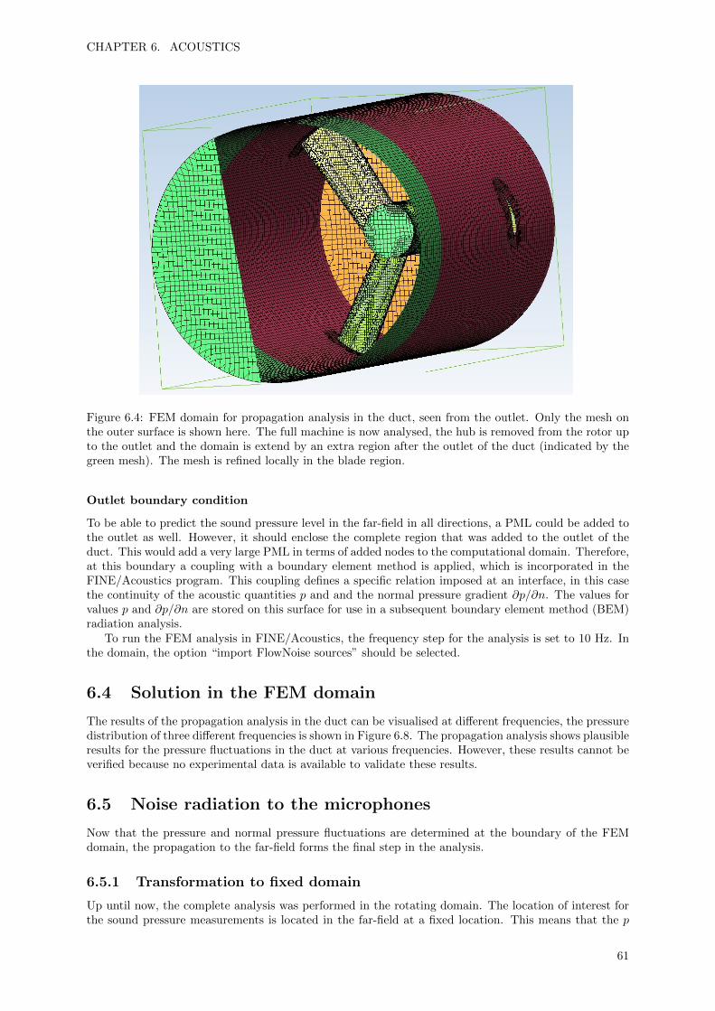
CHAPTER 6. ACOUSTICS
Figure 6.4: FEM domain for propagation analysis in the duct, seen from the outlet. Only the mesh onthe outer surface is shown here. The full machine is now analysed, the hub is removed from the rotor upto the outlet and the domain is extend by an extra region after the outlet of the duct (indicated by thegreen mesh). The mesh is refined locally in the blade region.
Outlet boundary condition
To be able to predict the sound pressure level in the far-field in all directions, a PML could be added tothe outlet as well. However, it should enclose the complete region that was added to the outlet of theduct. This would add a very large PML in terms of added nodes to the computational domain. Therefore,at this boundary a coupling with a boundary element method is applied, which is incorporated in theFINE/Acoustics program. This coupling defines a specific relation imposed at an interface, in this casethe continuity of the acoustic quantities p and and the normal pressure gradient ∂p/∂n. The values forvalues p and ∂p/∂n are stored on this surface for use in a subsequent boundary element method (BEM)radiation analysis.
To run the FEM analysis in FINE/Acoustics, the frequency step for the analysis is set to 10 Hz. Inthe domain, the option “import FlowNoise sources” should be selected.
6.4 Solution in the FEM domain
The results of the propagation analysis in the duct can be visualised at different frequencies, the pressuredistribution of three different frequencies is shown in Figure 6.8. The propagation analysis shows plausibleresults for the pressure fluctuations in the duct at various frequencies. However, these results cannot beverified because no experimental data is available to validate these results.
6.5 Noise radiation to the microphones
Now that the pressure and normal pressure fluctuations are determined at the boundary of the FEMdomain, the propagation to the far-field forms the final step in the analysis.
6.5.1 Transformation to fixed domain
Up until now, the complete analysis was performed in the rotating domain. The location of interest forthe sound pressure measurements is located in the far-field at a fixed location. This means that the p
61
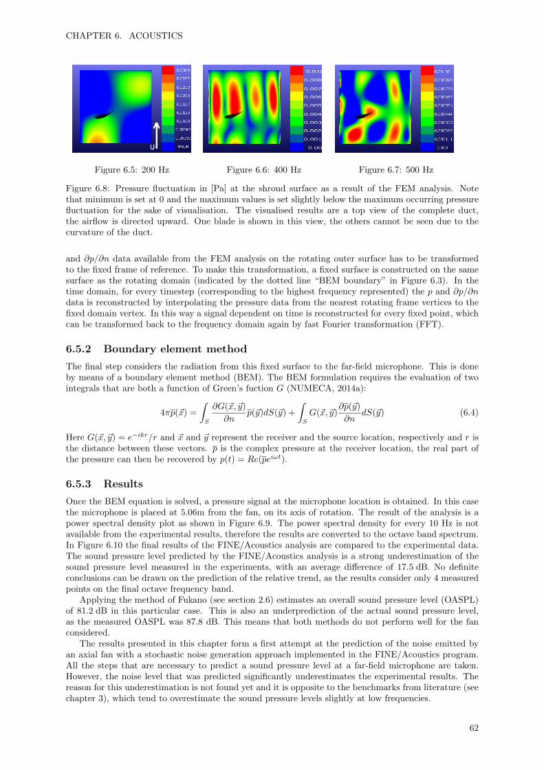
CHAPTER 6. ACOUSTICS
Figure 6.5: 200 Hz Figure 6.6: 400 Hz Figure 6.7: 500 Hz
Figure 6.8: Pressure fluctuation in [Pa] at the shroud surface as a result of the FEM analysis. Notethat minimum is set at 0 and the maximum values is set slightly below the maximum occurring pressurefluctuation for the sake of visualisation. The visualised results are a top view of the complete duct,the airflow is directed upward. One blade is shown in this view, the others cannot be seen due to thecurvature of the duct.
and ∂p/∂n data available from the FEM analysis on the rotating outer surface has to be transformedto the fixed frame of reference. To make this transformation, a fixed surface is constructed on the samesurface as the rotating domain (indicated by the dotted line “BEM boundary” in Figure 6.3). In thetime domain, for every timestep (corresponding to the highest frequency represented) the p and ∂p/∂ndata is reconstructed by interpolating the pressure data from the nearest rotating frame vertices to thefixed domain vertex. In this way a signal dependent on time is reconstructed for every fixed point, whichcan be transformed back to the frequency domain again by fast Fourier transformation (FFT).
6.5.2 Boundary element method
The final step considers the radiation from this fixed surface to the far-field microphone. This is doneby means of a boundary element method (BEM). The BEM formulation requires the evaluation of twointegrals that are both a function of Green’s fuction G (NUMECA, 2014a):
4πp(~x) =
∫S
∂G(~x, ~y)
∂np(~y)dS(~y) +
∫S
G(~x, ~y)∂p(~y)
∂ndS(~y) (6.4)
Here G(~x, ~y) = e−ikr/r and ~x and ~y represent the receiver and the source location, respectively and r isthe distance between these vectors. p is the complex pressure at the receiver location, the real part ofthe pressure can then be recovered by p(t) = Re(peiωt).
6.5.3 Results
Once the BEM equation is solved, a pressure signal at the microphone location is obtained. In this casethe microphone is placed at 5.06m from the fan, on its axis of rotation. The result of the analysis is apower spectral density plot as shown in Figure 6.9. The power spectral density for every 10 Hz is notavailable from the experimental results, therefore the results are converted to the octave band spectrum.In Figure 6.10 the final results of the FINE/Acoustics analysis are compared to the experimental data.The sound pressure level predicted by the FINE/Acoustics analysis is a strong underestimation of thesound pressure level measured in the experiments, with an average difference of 17.5 dB. No definiteconclusions can be drawn on the prediction of the relative trend, as the results consider only 4 measuredpoints on the final octave frequency band.
Applying the method of Fukano (see section 2.6) estimates an overall sound pressure level (OASPL)of 81.2 dB in this particular case. This is also an underprediction of the actual sound pressure level,as the measured OASPL was 87.8 dB. This means that both methods do not perform well for the fanconsidered.
The results presented in this chapter form a first attempt at the prediction of the noise emitted byan axial fan with a stochastic noise generation approach implemented in the FINE/Acoustics program.All the steps that are necessary to predict a sound pressure level at a far-field microphone are taken.However, the noise level that was predicted significantly underestimates the experimental results. Thereason for this underestimation is not found yet and it is opposite to the benchmarks from literature (seechapter 3), which tend to overestimate the sound pressure levels slightly at low frequencies.
62

CHAPTER 6. ACOUSTICS
0 100 200 300 400 500 6000
20
40
60
80
Frequency (Hz)
Sou
nd
pre
ssu
rele
vel
(dB
)
Figure 6.9: Power spectral density of the sound pressure level predicted at the microphone byFINE/Acoustics
0 100 200 300 400 500 6000
20
40
60
80
Frequency (Hz)
Sou
nd
pre
ssu
rele
vel
(dB
)
Figure 6.10: Comparison of the octave band sound pressure level predicted at the microphone byFINE/Acoustics and the measured experimental results
63

CHAPTER 6. ACOUSTICS
64

Chapter 7
Conclusions and Recommendations
The main objective of this research was to identify and evaluate a suitable technique for the predictionof broadband noise of axial fans for engineering purposes. This chapter presents the most importantconclusions that have been drawn from the research that was performed. Based on these conclusionsand practical experience gained during the performed research, some recommendations are presented.
7.1 Conclusions
Selected method
The literature review showed that to accurately predict noise, the acoustic source field has to be recon-structed. This field can be obtained directly from computationally expensive methods such as directnumerical simulation or large eddy simulation, but this is not (yet) feasible for engineering purposes.The stochastic noise generation and radiation (SNGR) method turned out to be able to provide a recon-structed acoustic source field based on the, computationally much cheaper, steady Reynolds-AveragedNavier-Stokes equations (RANS).
RANS simulations
The results of the simulations presented in chapter 5 show good agreement with experimental results,even though several simplifications of the geometry and domain have been applied. The most importantsimplifications are that the tip gap was not modelled and that the hub that extends throughout thecomplete domain. Several checks were performed to ensure that these simulations provide a reliableresult. The reduction of the residual of relevant flow parameters and the global residual were monitoredas well, showing good convergence behaviour. The discretisation error was estimated, showing acceptableresults. The flow field was inspected near the blade to investigate whether the flow did not contain anyirregularities and did not show any unexpected flow behaviour. The pressure and efficiency curves ofthe simulations show good qualitative and quantitative agreement to the measurements. In the standardoperation range of the fan the pressure coefficient is overpredicted by a maximum of 11% for the Spalart-Allmaras turbulence model. When effects of stall become important, the model does not perform well.The final analysis with the shear stress transport model, which is used for the consecutive acousticanalysis, shows an underprediction of 6.4% for the pressure coefficient, which is deemed an acceptabledeviation. Based on these results, the RANS analysis performed in FINE/Turbo can be used withconfidence as input for the acoustic analysis.
7.1.1 Acoustics
Source field reconstruction
Based on the input provided by the RANS simulation, an adaptive mesh was created to reconstruct theacoustic source field using SNGR. A convergence analysis showed that the adaptive mesh was refinedsufficiently to represent all the frequencies of interest on this mesh. The result of the acoustic sourcereconstruction by the SNGR method shows that the strongest sources are located in the region near thetrailing edge of the blade. Also, the sources increase in strength with increasing radius, with the strongest
65

CHAPTER 7. CONCLUSIONS AND RECOMMENDATIONS
sources located near the shroud, where the blade velocity is largest. This conforms with information andscaling laws found in literature.
FEM acoustic propagation analysis
The reconstructed sources are embedded in a finite element method (FEM) propagation analysis throughthe complete duct. To accurately represent the situation present in the conducted experiments, theextension of the hub is removed from this analysis and a so-called perfectly matched layer is added atthe inlet of the domain to represent an infinite duct. At the outlet the domain is extended outward, touse this surface for a far-field radiation analysis. The results of the FEM propagation show plausibleresults for the pressure fluctuations in the duct at various frequencies. However, these results could notbe verified because no experimental data was available to validate these results.
Far-field microphone noise prediction
The aim of the research was to predict the noise at a far-field microphone. The preliminary resultspresented in this report show a considerable underestimation of the noise levels measured in experiments.In the current analysis various simplifications and assumptions were made and thorough convergence andparameter influence studies are not performed yet. Therefore, no definitive conclusion can be drawn onwhether the method is a suitable technique for the prediction of broadband noise emitted by low-speedaxial fans. Additional research is required to resolve these issues.
7.2 Recommendations
Based on the conclusions presented in the previous section and practical experience obtained in thecomplete process, this section presents some recommendations for further research.
Validation of experiments
In this thesis a lot of effort was put in the prediction of aerodynamic performance using CFD. Thesepredictions were compared to experimental measurements and a large discrepancy between these resultswas initially discovered. This was assumed to be due to modelling or input errors in the CFD analysis.However, this turned out to be due to erroneous experimental values. It is recommended that, in everyCFD analysis in which results are compared to experiments, at least one experiment is repeated incooperation with the person conducting the CFD analysis. This is very informative for the CFD analystand ensures high quality experimental results.
Incompressible RANS analysis
The current research covers a compressible RANS analysis. In the particular case of low-speed axialfans, where the maximum Mach number typically does not exceed 0.2, an incompressible RANS analysisshould be of equivalent accuracy as the compressible code. Using an incompressible code could savevaluable time and storage and therefore streamline the complete process.
Thorough check of current analysis steps
The current analysis does not provide a correct quantitative prediction of the noise of low-speed axialfans. Mistakes could be made in one of the many steps performed in the analysis or there might still be aflaw in the Alpha-release of the software. As the time was limited in the current project and the acousticanalysis covers many steps that have been performed with an Alpha-release of the FINE/Acousticsprogram, it is recommended to check all these steps taken in the process thoroughly.
Mesh dependency
To ensure the quality of any prediction based on solution solved with a discretised system of equations,a mesh dependency study should be performed. In the time frame of this research, unfortunately thiscould only be conducted for the RANS analyses performed with the Spalart-Allmaras turbulence model.For the analysis performed with the SST model, for the DSNG source reconstruction and for the FEMpropagation analysis, a mesh refinement study should also be performed to ensure mesh independentresults in every step in the complete prediction process.
66
CHAPTER 7. CONCLUSIONS AND RECOMMENDATIONS
Geometry
Some simplifications have been made in the geometry. The hub has been extended from the rotor plane tothe outlet in the RANS analyses. This is most likely of minor influence on the aerodynamic performanceanalysis, but might influence the reconstructed turbulence field considerably. Another simplificationwas in the modelling of the tip of the blade, in the current analyses the tip gap was omitted. For theaerodynamic performance this leads to errors in the range of 5 to 10%. The influence on the generatednoise might be considerably larger, due to the leakage flow present at the tip.
Incident turbulence level
In this research, the incident turbulence level was set to a constant level of 5%. As mentioned inliterature, this might also be an important factor in the generation of noise in axial fans. Therefore, itis recommended to conduct a parameter study for this variable, to investigate the importance in thisparticular case.
Prediction of trends
As a first step in the usage of the DSNG method for the prediction low-speed axial fan noise, focussing onthe prediction of trends observed in experiments is recommended. Some scaling laws are observed in theoperation of fans, such as the scaling of the noise with the tip Mach number, this could be investigatedrelatively easily, by minor adjustments in the analysis settings.
Also, clearly different fans with respect to noise production can be tested to investigate if a relativedistinction between a ’silent’ and ’noisy’ fan can be obtained. If this is the case, the method can beincorporated in a design process, even though no absolute noise level may be predicted with confidence.
67

CHAPTER 7. CONCLUSIONS AND RECOMMENDATIONS
68

References
R. Aarts. A comparison of some loudness measures for loudspeaker listening tests. Journal of the AudioEngineering Society, 40(3):142–146, 1992.
G. A. Ashford. An unstructured grid generation and adaptive solution technique for high-Reynolds-numbercompressible flows. University of Michigan, 1996.
C. Bailly and D. Juve. A stochastic approach to compute subsonic-noise using linearized Euler’s equa-tions. In 5th AIAA/CEAS Aeroacoustics Conference. American Institute of Aeronautics and Astro-nautics, 1999.
J. P. Berenger. A perfectly matched layer for the absorption of electromagnetic waves. Journal ofcomputational physics, 114(2):185–200, 1994.
V. P. Blandeau and P. F. Joseph. Validity of Amiet’s model for propeller trailing-edge noise. AIAAjournal, 49(5):1057–1066, 2011.
D. Casalino and M. Barbarino. Stochastic method for airfoil self-noise computation in frequency domain.AIAA journal, 49(11):2453–2469, 2011.
I. B. Celik, U. Ghia, P. J. Roache, and C. J. Freitas. Procedure for estimation and reporting of uncertaintydue to discretization in CFD applications. Journal of Fluids Engineering-Transactions of the ASME,130(7), 2008.
M. Crocker. Handbook of noise and vibration control. John Wiley & Sons, 2007.
N. Curle. The influence of solid boundaries upon aerodynamic sound. Proceedings of the Royal Societyof London. Series A. Mathematical and Physical Sciences, 231(1187):505–514, 1955.
P. di Francescantonio, P. Ferrante, T. Deconinck, and C. Hirsch. Assessment of SNGR method for robustand efficient simulations of flow generated noise. In 19th AIAA/CEAS Aeroacoustics Conference.American Institute of Aeronautics and Astronautics, 2013.
P. Doak. Fluctuating total enthalpy as the basic generalized acoustic field. Theoretical and ComputationalFluid Dynamics, 10(1-4):115–133, 1998.
P. Ferrante. Flow-Noise analysis of a Car’s Mirror based on steady RANS simulation. NUMECA WebinarSeries, September 2014.
J. Ffowcs Williams and D. Hawkings. Sound generation by turbulence and surfaces in arbitrary mo-tion. Philosophical Transactions of the Royal Society of London. Series A, Mathematical and PhysicalSciences, 264(1151):321–342, 1969.
R. W. Fox and A. T. McDonald. Introduction to fluid mechanics, volume 7. John Wiley & Sons NewYork, 1985.
T. Fukano, Y. Kodama, and Y. Senoo. Noise generated by low pressure axial flow fans, I: Modeling ofthe turbulent noise. Journal of Sound and Vibration, 50(1):63–74, 1977a.
T. Fukano, Y. Kodama, and Y. Takamatsu. Noise generated by low pressure axial flow fans, II: Effectsof number of blades, chord length and camber of blade. Journal of Sound and Vibration, 50(1):75–88,1977b.
69
REFERENCES
T. Fukano, Y. Kodama, and Y. Takamatsu. Noise generated by low pressure axial flow fans, III: Effectsof rotational frequency, blade thickness and outer blade profile. Journal of Sound and Vibration, 56(2):261–277, 1978.
N. Hakimi. Preconditioning methods for time dependent Navier-Stokes equations: Application to Envi-ronmental and Low Speed Flows. PhD thesis, Vrije Universiteit Brussel, Pleinlaan 2, B-1050, Belgium,December 1997.
C. Hirsch. Numerical Computation of Internal and External Flows: The Fundamentals of ComputationalFluid Dynamics, volume 1. Butterworth-Heinemann, 2 edition, 2007.
Howden Netherlands b.v. 16-07.002 Aerodynamic and acoustic performance testing of Howden coolingfans. 2014.
M. Howe. Contributions to the theory of aerodynamic sound, with application to excess jet noise andthe theory of the flute. Journal of Fluid Mechanics, 71(04):625–673, 1975.
A. Jameson, W. Schmidt, and E. Turkel. Numerical solutions of the euler equations by finite volumemethods using runge-kutta time-stepping schemes. AIAA paper, 1259:1981, 1981.
W. Jones and B. Launder. The prediction of laminarization with a two-equation model of turbulence.International journal of heat and mass transfer, 15(2):301–314, 1972.
F. Kameier and W. Neise. Rotating blade flow instability as a source of noise in axial turbomachines.Journal of Sound and Vibration, 203(5):833–853, 1997.
G. Kirchhoff. Zur Theorie der Lichtstrahlen. Annalen der Physik, 254(4):663–695, 1883.
R. H. Kraichnan. Diffusion by a random velocity field. Physics of Fluids, 13(1):22–31, 1970.
P. K. Kundu, I. M. Cohen, and D. R. Dowling. Fluid Mechanics. Elsevier Inc., 2012.
A. Lafitte, T. L. Garrec, C. Bailly, and E. Laurendeau. Turbulence generation from a sweeping-basedstochastic model. AIAA journal, 52(2):281–292, 2014.
M. Lighthill. On sound generated aerodynamically. Proceedings of the Royal Society of London. SeriesA. Mathematical and Physical Sciences, 211(1107):564–587, 1952.
A. S. Lyrintzis. Surface integral methods in computational aeroacoustics—from the (cfd) near-field tothe (acoustic) far-field. International journal of aeroacoustics, 2(2):95–128, 2003.
F. R. Menter. Two-equation eddy-viscosity turbulence models for engineering applications. AIAA jour-nal, 32(8):1598–1605, 1994.
M. P. Norton. Fundamentals of noise and vibration analysis for engineers. Cambridge university press,1989.
NUMECA. FINE/Acoustics v5.2.3 Manual. July 2014a.
NUMECA. AutoGrid5 v9: User Manual. September 2014b.
NUMECA. FINE/Turbo v9.1: Theorectical Manual. September 2014c.
Y. Pao. Structure of turbulent velocity and scalar fields at large wavenumbers. Physics of Fluids, 8(6):1063–1075, 1965.
S. B. Pope. Turbulent flows. Cambridge University Press, 2000.
A. Powell. Theory of vortex sound. The journal of the acoustical society of America, 36(1):177–195,1964.
D. Russel. Acoustics and vibration animations. URL: http://www.acs.psu.edu/drussell/Demos/rad2/mdq.html,2001. Accessed June 6th, 2014.
D. Russell. On the sound field radiated by a tuning fork. American Journal of Physics, 68(12):1139–1145,2000.
70
REFERENCES
F. G. Schmitt. About boussinesq’s turbulent viscosity hypothesis: historical remarks and a direct eval-uation of its validity. Comptes Rendus Mecanique, 335(9):617–627, 2007.
I. Sharland. Sources of noise in axial flow fans. Journal of Sound and Vibration, 1(3):302–322, 1964.
D. N. Sørensen. Minimizing the trailing edge noise from rotor-only axial fans using design optimization.Journal of sound and vibration, 247(2):305–323, 2001.
P. R. Spalart and S. R. Allmaras. A one-equation turbulence model for aerodynamic flows. RechercheAerospatiale, 1:5–21, 1994.
P. R. Spalart and C. L. Rumsey. Effective inflow conditions for turbulence models in aerodynamiccalculations. AIAA journal, 45(10):2544–2553, 2007.
T. Von Karman. Mechanische Ahnlichkeit und Turbulenz. Proc. Third Int. Congr. Applied MechanicsStockholm, pages 85–105, 1930.
D. C. Wilcox. Turbulence Modeling for CFD. DCW Industries, Incorporated, 1993.
71

REFERENCES
72

Appendix A
Experimental set-up
This appendix covers the experimental set-up and the procedures followed to obtain the experimentalresults. The experimental values are all obtained at the Howden Netherlands B.V. (HNL) testing facility.A schematic overview and a photograph of the complete set-up are shown in Figure A.1 and Figure A.2respectively. The set-up is a free inlet, free outlet configuration, this means that there is no significantducting at the inlet or outlet side of the fan. The diameter of the test section 1845 mm, making itpossible to test fans up to a diameter of 1829 mm (6 ft). The reason for this large test section is thatthe scaling using dimensionless numbers is not completely flawless. As industrial cooling fans can reachdiameters of more than 10 m, the tests take place at this large scale to reduce the errors made in thisby scaling these results.
The HNL test set-up consists the following parts, indicated in Figure A.1:
1. Tunable inlet valve
2. Booster fan
3. Outlet guide vanes
4. Settling screens
5. Flow nozzle
6. Electric motor
7. Settling screens
8. Test fan
During the standard aerodynamic performance measurements the following variables are directly mea-sured:
Pressure drop over the flow nozzle (#5)
Fan static pressure (FSP)
Fan shaft torque
Fan speed
Ambient temperature
Relative humidity
Atmospheric pressure
Using these variables the following additional relevant parameters are determined:
Air volume flow (Q)
Fan shaft power (Pshaft)
Air density (ρ)
73

APPENDIX A. EXPERIMENTAL SET-UP
Figure A.1: Experimental set-up, the dotted line box at the right shows the computational domain(From: Howden Netherlands b.v. (2014)).
Fan tip speed (vtip)
Flow coefficient (Cf )
Pressure coefficient (Cp)
Fan static efficiency (ηts)
Flow rate determination
Using the measured static pressure drop over the flow nozzle, the volume flow can be determined usinga nozzle factor fnozzle, which is determined by a calibration procedure:
Q = fnozzle =
√2∆pnozzle
ρ(A.1)
Fan static pressure measurement
To measure the fan static pressure (FSP = p2 − p01), an array of three Pitot tubes connected is used tomeasure the total pressure in the settling chamber between the settling screens (7) and the fan itself (8).This array is connected to a digital differential pressure transducer, where it is compared to the outletstatic pressure.
Rotational speed, torque and power
At the fan shaft, the shaft torque (T [Nm]) is measured using a torque meter and the rotational speed(RPM or Ω [rad/s]) is measured using an simple induction sensor, which registers the passage of a bolthead attached to the shaft, giving an analog pulse at each passage. With this information, the shaftpower can be determined by:
Pshaft = TΩ (A.2)
Measurement accuracy
The Howden test facility is calibrated regularly, to meet the requirements set for all sensors as definedin Table A.1.
74
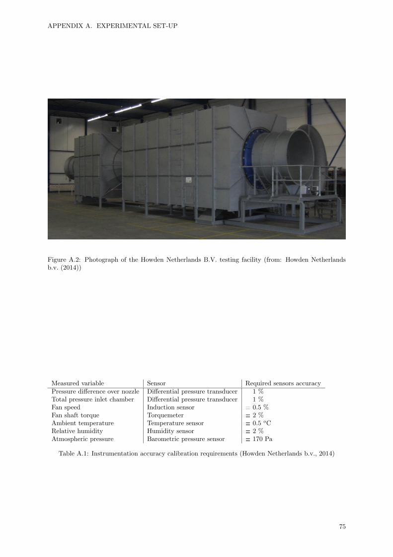
APPENDIX A. EXPERIMENTAL SET-UP
Figure A.2: Photograph of the Howden Netherlands B.V. testing facility (from: Howden Netherlandsb.v. (2014))
Measured variable Sensor Required sensors accuracyPressure difference over nozzle Differential pressure transducer ± 1 %Total pressure inlet chamber Differential pressure transducer ± 1 %Fan speed Induction sensor ± 0.5 %Fan shaft torque Torquemeter ± 2 %Ambient temperature Temperature sensor ± 0.5 oCRelative humidity Humidity sensor ± 2 %Atmospheric pressure Barometric pressure sensor ± 170 Pa
Table A.1: Instrumentation accuracy calibration requirements (Howden Netherlands b.v., 2014)
75

APPENDIX A. EXPERIMENTAL SET-UP
0 0.05 0.1 0.15 0.2 0.25 0.30
0.05
0.1
0.15
0.2
Flow coefficient (Cf )
Pre
ssu
reco
effici
ent
(Cp)
Booster onBooster off
Figure A.3: Measurement of the test fan performed at the HNL testing facility. Turning the booster fanoff should result in partially overlapping measurements, which is demonstrated here.
A.1 Measurement procedure
The first measurements are performed with the booster fan turned on and the tunable inlet valve com-pletely opened, once the flow variables have stabilised, a first measurement is conducted, which averagesall the measured variables over a timespan of 30 seconds. For the following points this procedure isrepeated, closing the inlet valve step by step. This way the volume flow decreases and the FSP increases,moving left over the fan curve. Once the inlet valve is almost completely closed, the booster fan is turnedoff and the inlet valve is opened up again completely. This causes the flow rate to increase again andthe fan static pressure to drop, moving right on the fan curve again. From this point on, the inlet valveis closed step by step again, if the measurements are performed correctly, the first few measurementswithout booster fan activated, should overlap the last measurements with the booster fan turned on,which is shown in Figure A.3.
A.2 Comparison of new and old experimental results
As explained in chapter 5, the results obtained in the two sets experiments were not consistent. Thedifferences could not be explained to this day, but it is assumed that the second set of experimentalvalues are correct. The first set of experiments was conducted with the same set-up a long time ago,but the complete installation was located outside at the time of these measurements and the specificmeasurement conditions could not be determined. The difference in the measurements obtained is shownin Figure A.4.
76

APPENDIX A. EXPERIMENTAL SET-UP
0 0.05 0.1 0.15 0.2 0.25 0.30
0.1
0.2
0.3
Flow coefficient (Cf )
Pre
ssure
coeffi
cien
t(C
p)
NewOld
0 0.05 0.1 0.15 0.2 0.25 0.30
20
40
60
80
100
Flow coefficient (Cf )
Sta
tic
effici
ency
(ηts
)NewOld
Figure A.4: A comparison of the two sets of experimental results
77

APPENDIX A. EXPERIMENTAL SET-UP
78

Appendix B
Mesh generation in AutoGrid
In this appendix, the procedure of generating a numerical mesh used for the CFD calculations is elab-orated. The geometry is first fully defined in AutoBlade as described in section 5.2. This geometry isthen imported in AutoGrid5, in this program the complete computational grid can be automaticallygenerated.
In the detailed mesh control grid level is set to medium and the number of grid levels is set to 3.After this, the following settings are applied in the program using the row wizard. Options not statedhere are kept at their default values.
1. Row type: Axial Fan
Periodicity: 3
Rotation speed: -500 RPM
2. No hub and tip gap or fillets are applied.
3. Layer control
Spanwise grid point number: 93 for SST, 57 for SA.
Wall cell width: 1 · 10−5 m
4. Blade to blade control
Level: 0
The blade to blade mesh topology is shown in Figure B.3, once this mesh does not show any flaws (e.g.unconnected nodes or very skewed cells), the three-dimensional mesh is generated. The quality reportsgenerated for the employed meshes for the SA and SST models are shown in Figure B.4 and B.5. Theaspect ratio is defined for each face in the mesh by calculating the mean of the lengths of the opposingsides and taking the ratio of these means as shown in Figure B.1. The expansion ratio is a measure forthe size difference of cells in a particular direction, defined as shown in Figure B.2. Both the aspect ratioand the expansion ratio should be kept as small as possible for an accurate CFD analysis. The skewnessis defined as the minimum angle between the edges of a cell (for angles α larger that 90 degrees it ismeasured as 180 − α) The skewness value as close to 90 degrees as possible. The majority of the cellslie within the first bin of the grid quality report and no negative cells are detected by the program, thusthe meshes are considered appropriate for the analyses performed in this thesis.
79

APPENDIX B. MESH GENERATION IN AUTOGRID
Figure B.1: Aspect ratio definition (From: NUMECA (2014b))
Figure B.2: Expansion ratio definition (From: NUMECA (2014b))
d
thetaa
dm/r
thetaa
MM-THETMM-THETTATA
Figure B.3: Generated blade to blade mesh
80

APPENDIX B. MESH GENERATION IN AUTOGRID
Figure B.4: Grid Quality report for the mesh used for the simulations performed with the Spalart-Allmaras (SA) turbulence model
Figure B.5: Grid Quality report for the mesh used for the simulations performed with the shear stresstransport (SST) turbulence model
81

APPENDIX B. MESH GENERATION IN AUTOGRID
82

Appendix C
CFD analysis settings
This appendix describes the detailed settings of the CFD calculations performed with the FINE/Turboprogram. The grid is generated in AutoGrid with the geometry that is defined in AutoBlade.
The settings defined in FINE/Turbo are listed below. These are the settings for the final calculation,performed with the shear stress transport turbulence model, that is used as input for the acoustic analysis.The input that changes for the Spalart-Allmaras fan curve calculations is listed in Table C.1.
1. Configuration
Fluid Model - Air (Perfect)
Flow Model
Mathematical Model - Turbulent Navier-Stokes
Modelling of Turbulence - Shear Stress Transport (SST)
Characteristic Length - 0.347 m (Chord length)
Characteristic Velocity - 47.43 m/s (Tip speed)
Characteristic Density - 1.19 kg/m3
Tref = 291.07 K, pref = 99426 Pa
Rotating Machinery - Rotational speed = -495.35 RPM
2. Boundary Conditions
Inlet - Velocity Components
Vz = 6.7225 m/s
Tstatic = 291.07 K
k = 0.1695 m2/s2 (With I = 0.05 and k = 3/2(UrefI)2
ε = 0.08955 m2/s3 (With ε = c3/4µ k3/2l−1 )
Outlet - Static pressure imposed - Constant - 99426 Pa
Periodic - Matching
Solid - Adiabatic - Constant Rotation Speed - Pressure from Extrapolation
Hub - Rotational speed: -495.35 RPM
Shroud - Rotational speed: 0 RPM
Blade - Rotational speed: -495.35 RPM
3. Numerical Model
CFL number: 3
Number of grid levels: 3
Coarse grid initialization active
Preconditioning parameters
Method: Hakimi
β∗ coefficient: 3
Characteristic velocity: 47.43 m/s
Local velocity scaling active
83

APPENDIX C. CFD ANALYSIS SETTINGS
Multigrid parameters
Scheme definition: Sweeps increase on higher level
Maximum cycles per grid level: 300
Convergence criteria on each grid level: -4.0
4. Initial solution - for turbomachinery
Constant estimated static pressure: 97500 Pa
k = 0.1695 m2/s2
ε = 0.008955 m2/s3
5. Computation Steering
Max. # of iterations: 1200
Global residual convergence criteria: -6.0
Solver precision: Double
Expert parameters
Multigrid under-relaxation factor (ALFAMG): 0.7
Clipping value for µT
µ (MUCLIP): 50000
The fan curve calculations are performed with the Spalart-Allmaras model, a one equation model,for the sake of calculation speed. The input for this model is only the turbulent viscosity (νT ), instead ofk and ε. This parameter is estimated using νT /ν = 2.5 as recommended for internal flows (NUMECA,2014c) and is set constant to νT = 3.35 · 10−5 m2/s. The other variables that are changed for the curvesimulation to correspond to measured data are shown in Table C.1.
# Rotational Speed [RPM] Vz[m/s]1 489.18 3.682 489.10 5.203 487.15 7.384 486.84 9.055 486.92 10.456 488.01 11.657 487.70 12.778 488.24 13.789 488.87 14.53
Table C.1: Changed input values for fan curve CFD calculations
84
Appendix D
Discretisation error estimation
The discretisation of the equations described in chapter 4 leads to inevitable errors, but if the grid iscarefully constructed the results should improve towards the analytical solution. To see if the CFDanalysis shows the correct convergence behaviour a grid convergence study is performed. The procedureapplied here follows the approach of Celik et al. (2008). Using three grids, an estimate is made of theorder of convergence, with this an extrapolation to the analytical solution can be made and the numericalerror that is made can be estimated.
First, three grids are created. Here the coarsest grid represents the grid that is used for the calculationsreported in chapter 5. The other two grids are refinements of this grid, increasing the number of nodesby using a refinement factor of approximately 1.3 in each direction, satisfying the minimum decrease incell size that is deemed appropriate for a grid convergence study. For grid i a representative grid sizecan be determined using:
hi =
[1
Ni
Ni∑k=1
(∆Vk)
]1/3
(D.1)
Here ∆Vk is the volume of the kth cell and Ni the total number of cells on the ith grid. Between twogrids, the refinement factor is defined as rij = hi/hj . As the sum of the volumes is equal for everygrid analysed here, this term cancels out. For every variable φ, the solution of this variable on a gridis denoted as φi and the difference of the solutions on two grids is denoted as εij = φi − φj . For threegrids, the apparent order can then be determined using the expression:
p =1
ln(r21)ln|ε32/ε21| (D.2)
When the apparent order is determined, the extrapolated values can be determined using:
φijext =(rpijφj − φi
)/(rpij − 1
)(D.3)
The approximated and extrapolated error are calculated respectively as:
eija =
∣∣∣∣φj − φiφj
∣∣∣∣ and eijext =
∣∣∣∣∣φijext − φjφijext
∣∣∣∣∣ (D.4)
Finally, the grid convergence index (GCI) can be determined:
GCIijfine =1.25eijarpij − 1
(D.5)
For this grid refinement study, three parameters that are of importance for the final solution arechosen: the fan static pressure (FSP), the total-to-total efficiency (ηts) and the shaft power (Pshaft).Using equations D.2 to D.5, the grid refinement is performed for these three parameters. An overviewof the results of the grid refinement study is shown in Table D.1. The maximum grid convergence erroron the grid used for the calculations is estimated to be 2.75%, which is considered to be an acceptablelevel for engineering purposes.
85

APPENDIX D. DISCRETISATION ERROR ESTIMATION
φ =FSP[Pa] φ = ηtt[%] φ = Pshaft[W]N1, N2, N3(·106) 11.2, 4.8, 2.0 11.2, 4.8, 2.0 11.2, 4.8, 2.0r21 & r32 1.33 1.33 1.33φ1 63.5 85.1 4817φ2 59.2 85.2 4737φ3 58.3 84.0 4717ε32 -0.9 -1.2 -20ε21 -4.3 0.2 -80p 5.5 6.5 4.8φ21ext 64.7 85.0 4845φ32ext 59.4 85.5 4744e21ext 1.79% 0.043% 0.57%e31a 8.20% 1.23% 2.08%CGI31
fine 2.75% 0.29% 0.89%
Table D.1: Grid refinement results
86