SPE-H ~km=f=

, SPE 20020

Prediction of Steamflood Performance in Heavy Oil ReservoirsUsing Correlations Developed by Factorial Design MethodC. Chu, Texaco Inc.

SPE Member

:opyright 19S0, Soolefy of Petroleum Engineers Inc.

rhls paper wee prepared for presentation at the SOthCalifornia Regional Meeting held iti Ventura, California, April 4-S, 1990.

rhls paper was selected for presentation by an SPE Program Committee followingreviewofinformationContainedInm *StraCtSubrnitttiW theauthor($).mntemaof the P*r.IS presented, have not been reviewed by the Society of Petroleum Engineers and are subject to correofionby the author(s), The material, ae presented, does not necessarily reffedmy positionof the So.5efy of Petrolsum Englnears, its officsra, or membara. Papers presented at SPE meetings ara subjeotto publicationreview by EditorialCommittees of the Society>fPetroteumEnginwm. Permissionto copyis restrictedto en abstractof notmofe than SW words, Illusfraticmsmay notbe copied.The abstractshouldcuntairrconspicuousscknoWdgmWt]f where and by whom the paper la presented. Write Publicalkrns Manager, SPE, P.O. Sox 8S3SS8, Richardson, TX 7SOW-W3S. Telex, 7S09S9 SPEDAL.

with steamflood design and operating variables such as pattern

By using the factorial design method, statistically significantsize, steam injection rate, and steam quality. With these

correlations have been developed which enable one to predictquantities known, one can use the coI relations hereby

steamflood performance in terms of project life, oil recoverydeveloped to predict steamflood performance in regard to

The effects of variousproject life, oiI recovery and cum~lative Steam-oi’ ‘atio

and cumulative steam-oil ratio.reservoir rock and fluid properties and steamflood design and

(SOR).

operating variables on steamflood performance were

disousssad.In 1980 Gomaal developed a set of correlation charts forpredicting oil recovery and cumulative oil-steam ratio,emphasizing the effects of steam quality, mobile oilsaturation, reservoir thickness and net-gross ratio. One

The ideal way of predicting reservoir performance underconspicuous absence in the independent variables included in

steamflood is through numerical simulation. However, thishis work is the oil viscosity which could greatly affect the

approach may not be aiways feasibie due to either the iack of asteamflood performance. Gomaa’s method uses graphical

reiiabie thermal simuiator or the lack of quaiified personnelsolutions which usuaily iaok preoision because the reading of

to run the simulator. In some instances, such as estimation ofvalues from a chart is subject to the user’s judgment. The

oil reserves, screening thermal prospects or makingerrors will be compounded if several charts needed to be readto obtain the answer. In his method, finding the oii recovery

preliminary engineering design, detailed simulation may notbe warranted. Besides, early in the development of a detailed

requires the use of no iess than four charts.

simulation, a simple method of predicting reservoirperformance wiii provide a means of comparison. Under aii

ASWMPllQl!&

these circumstances, some correlations which allow the 1.prediction of steamflood performance without resorting to

The reservoir is horizontal, with no dipping.

numerical simulation will be useful. The purpose of this 2.work Is to develop such correlations. The end result of this

The resewoir is homogeneous throughout the entire

study is a simple ocrmputer program, written in BASIC, whichthi&ness, with no intervening shale breaks.

can be used to predict steamflood performance in heavy oiireservoirs (Appendix A).

3. There is neither gas cap at the top nor free gas insidethe oil sand.

A large amount of simulation by use of a three-dimensional ~numerical model has been made in this work so that the users “

There is no water sand underneath the oil sand.

of the correlations can predict steamflood performance 5.without the expense of doing simulation. The independent

The oil is sufficiently heavy to be adequately

variables used in the correlations include reservoir rock andrepresented by a single hydrocarbon component which

fluid properties such as reservoir thickness, porosity,is non-volatile.

permeability, initiai oil saturation, and oil viscosity, aiong

I

or

PREDICTIONOFSTEAMFLOODPERFORMANCEINHEAVY .

OILRESERVOIRSUSINGCORRELATIONSDEVELOPEDBYFACTORIAL2 DESIGNMETHOD SPE 20020

6. Single sand operation is assumed, with no interventionfrom sands above or beiow.

The foiiowing are used as Independent variables for the7. Repeated 5-spot patferns are assumed. correlation:

8. Constant steam injection rate and constant steam quality Reservoir rock and fluid propertiesare assumed throughout the project, with no tapering ineither injection rate or steam quaiity. Thickness, h, ft - gross thickness is used

Porosity, s, % bulk volume - measured based on9. Two or more steam stimulation cycles are assumed in gross thickness Permeability, k, md

the initial part of the steamflood. The slug size is Oil viscosity, p, cp - oil viscosity at 90”F10,000 bbls [1589.9ms] of steam for each cycie. The {3.2.2”C}is usedcycie length is 182.5 days. The number of cycies needed Oil saturation, SO,YO PV - initiai oil saturation at theis determined by the movement of the heat front, start of the steamfbodwhether or not heat bridge-over is forthcoming in thefoilowing haif-year period. Steamflood design and operating variables

10. The steamflood is terminated when the instantaneous Pattern size, A, acre - This refers to 5-spotratio between heat injection and oil production is patternsequivakrnt to an SOR of 10 B/B, [M31M3] the steam Steam injection rate, is, B/D - steam at 366° Fbeing 60 Y. quality at a saturation temperature of [185.6”C] is used Steam quality, fg , %366°F [185.B”C].

11. The steamflood performance is measured at that cutoffpoint. Any additional recovery by using hot waterflood, Since there are 8 factors, a total of 2e = 256 runs wili beinfill drilling, etc., is not considered. needed for a complete two-level factorial design. To minimize

Whereas the data are obtained from Kern River Field,the number of runs without sacrifice of information

California, the resuits should apply to other horizontalobtainable from the design, a 1/4 replicate was used which

homogeneous heavy oil reservoirs with properties nol too farcalls for 28 = 64 runs. According to Box and Hunter4, a

outside the ranges covered by this work.specific design wiil be needed to assure that all the maineffects and two-factor interactions will be clear of oneanother. That particular design calls for equating X7 with theproduct XI X2X3 u and eqUating xs with the product XI X2 xs

The factotial design method chooses the values of independent xs. To assure that these four-factor interactions will be

variables in a pre-determined fashion. in the terminology of negligible, the variables were reordered before being subject

the factorial design, the independent variables, normaliy after to transformation.

some transformation, are called factors. Two or more levelsof each factor are cho8en and the combinations of the levels The following equations define the transformed variables such

are used for experimentation. A factorial design refers to a as x1, X2 , etc., used for the factorial design in terms of the

particular combination of factor levels (Daviesp). The originai independent variables such as So, V, etc., and vice

advantage of using the factorial design method is that the versa:number of experiments (or simulation runs) can beminimized by using a systematic choice of variablecombinations. While this method has been applied mainly to SO-50experiments in biological, agricultural, medical and chemical xl = so= 50 + 5 xlresearch, it did find application in the study of fireflood(Sawyer et al.s).

T

The use of factorial design methods for development ofp -7000

X2 =steamflood design correlations involves the following steps:

K = 7000 + 2500 X2=0

1. Choose primary variables that have infiuence on steamfloodperformance

h-80)(3 a h= 80 + 20 x3

2. Transform the variablesT

3. Choose the factorial designi* -300

X4- i*= 300 + 50 X4

4. Make simulation runs and obtain the steamflood 50

performance variables for each run.A -2.6

5. Analyze the resuitsX5 9 A= 2.6 + 0.3 X5

x

-—

s

SPE 20020 CHIEHCHU 3—.——..——

fg -55)@* fg= 55 + 15 X6

7

k -3500X8 = k= 3500 + 750 X8

-z6-

It is obvious that the above equations are in the followingform:

V-a.X9 %~+al x

atThe value of x represents.the average value of V. The value ofal is meant to represent 1/4 of the range of V so that the valueof V will vary throughout the normally expected range when xchanges from -2 to +2.

The values of ~ and al for So, p, h, 1$,A, and a were estimatedfrom data on 60 steamflood projects in Kern River Field,California compiled by Restinas. Those fork and fg were based

on data from the history match paper by Johnson, et alG,

There was only one exception, namely, the al valUe for fg,whfch was purposely increased so as to obtain a fair indicationof the effect of steam quatity on steamflood performance.Gomaal indicated that the heat utilization factor increaseswith steam quality, reaches a maximum at approximately40% quality, and decreases when steam quality increasesfurther,

Based on the above equations, the factor levels are given inTable 1.

The fractional factorial design in terms of the transformedvariables, xl, X2, etc., is shown In the upper part of Table 2,namely, Runs 1-64. Some reflection will show that thefollowing substitutions, called for by Box and Hunterq, haveindeedbeen made:

)(7-X1)(2X3X4 )fs9xlx2x5)f5

10 obtain quadratic (second-order) effects of the variables,17 more runs were added. Whereas each variable in Runs1-64 assumes either -1 (the low level) or +1 (the highlevel), al! the vadables assume the O level, at the center ofall the variations, In Run 65. In Runs 66-81, each variablein turn slaps out SIfongthe coordinate axes to -2 and +2, withall other variables remahring at the O level. These runscombined with the first 64 runs form a non-orthogonalcomposite factorial desfgn as shown in Table 2.

A three-dimensional numerical model was used fOrsimulation. The input data for the primary variablecorresponding to the composite factorial design in Table 2 areobtained from Table 1. The rest of the input data are given inAppendix B.

Each run was terminated at the time when the instantaneoussteam/oli ratio is 10.0 B/B [Ms f/M3] for a 60% qualitysteam. Since steam quality varfes with the runs, the cutoffpoint is determined by the following equation:

Oil production is (hf + htg fg)rate =

10.0 (hf + hfe x 0.60)

where hf and htg are sinthalpy of saturated liquid water andlatent heat of vaporization at 366.0°F [185.6”C],respectively.

This determines the project life, the oil recovery and thecumulative SOFtt the cutoff point.

SIs of Rer@s

The entire set of 81 runs is used to obtain the main effect, bo,

the linear effects, bl ,...be, the second-order interactions,

btz,... bTs, and the quadratic effects, bl 1,...be8 In thefollowing equation:

Y = b.+ bl XI + ...... + bij x6

+ blz XI X2 + . . . . + b7sx7xe +bll X12 + .... +

bsaxsz

The response variable y may refer to project life, oilrecovery or cumulative SOR, as the case may be. The.coefflnents bo, bI, etc., are obtained by the method given inDavies? and are given in T~e 3“

Analysis of variance was appliad to the above equation. Theresults are summarized in Table 4. This table includes Fvalues, tall area, 9’o variation explained by the model, and theresidual standard deviation expressed as a percentage of theresponse mean. The tail area denotes the probability thatthere Is no correlation between the lndepafrdent and dependentvariables. The term called % variation explained by themodel Is also known as rz, or r-square. This is oftenconsidered as the most meaningful statbth since it gives us ameasure of the usefulness of the prediction (Dowdy andWeardenT). All four quantities Ibted in Table 4 show that theequation is statistically significant.

OF EESULK

The correlations developed here enable us to predict theeffects of various rock and fluid properties and steamflooddesign and operating vadSbfSSon SteamfbOd p6tfO~anCS. hthe foltowing dbcussbns, the varlabfas are varied, either oneat a time or two at a time, while all the other variables arehetd constant at the O factor levels. For exampfe, if the Initial

I*-

I

PREDtCTtONOFSTEAMFLOODPERFORMANCEINHEAVY .

OILRESERVOIRSUSINGCORRELATIONSDEVELOPEDBYFACTORIAL4 DES(3N~ SPE 20020

oI! aaturatton Is to be varied, the viscosity is held at 7,000 cpP.O Pas] and thickness is held at 80 ft [24.4m], etc.

Ie VafjgMQg

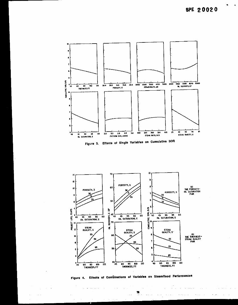
Figures 1-3 show the effects of the 8 independent variableson project life, oil recovery and cumulative SOR,respeotivefy. Each figure consists of 8 subfigures. The first5 subflgures refer to reservoir rock and fluid properties,namely, thickness, poroslt% permeability, oil viscosltY and~nitia[ oil saturation. The remaining 3 subfigures refer tosteamflood design and operating variables, namely, patternsize, steam rate and steam quality.

1. Project Life (Figure 1)

The most influential variable among the various reservoirproperties Is reservoir thickness. Project life almost triplesas thickness changes from 40 ff [12.2M] to 120 ft [3&6M].The next influential is 011saturation, which is followed byporosity. Increases in oil saturation or porosity will lengthenthe project life nearly propationately.

Permeability and oil viscosity have only minor influence onproject life. It should be noted that, since this work is basedon statlstkal treatment, each curve carries with it a band ofuncertainty. Because of this, the shallow maximum in theeffect of permeability and the shallow minimum in the effectof oil viscosity, as seen in this figure, may not be entirelysignificant. No belaboring was, therefore, made on theshapes of these cuwes and other cuwes in the followingfjgures wherever the responses appear to be rather minor.

All the three steamflood design and operating variables haveprofound influences on project life. Project life is nearlyproportional to pattern size and almost inverselyproportional to steam rate, Besides, project life is alsoshortened to some extent with higher steam quality.

2. Oil Recovery (Figure 2)

The most influential variable is the initial oil saturation. Itshould be noted that, whereas the oil recovery increasesalmost proportionately with the initial oil saturation, theremaining oil saturation aK& steamflood is almost unchanged.For example, with SO = 40%, the predicted oil recovery is44.2% of the OIP. The remaining oil saturation Is, then, 40 x(1-0.442) = 22.3Y0. If SO = 60Y0, the predicted oilrecovery is 60.4%, The remaining oil saturation is 60 x(1-0.604) = 23.7%. The increase In the remaining oilsaturation is a measly 23.7 - 22.3 = 1.4% PV when theInitial oil saturation is increased by 60-40 = 20% PV.

Other influential variables Include porosity and oil viscosity.Oil recovery increases with an Increase In porosity or adecrease In oil vlsccsity. The effect of resewoir thickness onoil recovery Is mlnlmal within the range of variationinvestigated, and when all the other variables are kept at theO factor level, e.g. steam quality = 557., etc.

Although the steamflood design and operating variables haveprofound Influences on project life, their influences on oilrecovery are rather insignificant, in the ranges used in thiswork and when one variable Is taken at one time with all theother variables kept at their respective O factor levels. Thispoints out the unfortunate fact that oil recovery Is governed

mainly by how much oil there is in the resewoir and howmobile the oil is. Judkbus choke of pattern size, steam rateand steam quality will help to enhance the oil recovery but toa much less extent than Is hoped to be.

I 3. Cumulative SOR (Figure 3)

The most influential variable is again the initial oilsaturation. With the same amount of steam, more oil will beproduced with a higher initial oil saturation, thus loweringthe cumulative SOR.

The cumulative SOR is also greatly influenced by reservoirthickness and oil vlecosity. As mentioned prevbusly, theeffect of thickness on oil t ~covery is minlmaL However, toobtain the same level of oil recovery, it b necessary to usemore steam in a thinner reservoir sc as to compensate for thegreater heat loss to the overburden and underburden.Cumulative SOR increases with oil viscosity because moreheat is needed to improve the oil mobility needed forproduction.

The fact that the cumulative SOR decreases with an increase insteam quality prompts us to see if the heat input per unitvolume of oil produced remains the same with a change insteam quatity. This was found to be true especially when thesteam quality is 55Ye or above, even though the cumulativeSOR changes to a great extent as the steam quality varies.

I Ef.mfs of @nkhmms of ,daklest

With 8 independent variables, there will be 8 x 7 = 56combinations if two variables are varied at a time. It willserve no purpose if the effects of all the combinations of thevariables on steamflood performance are included in thiswork. Rather, only two combinations have been selected to bediscussed, namely, the porosity-oil saturation pair and thethickness-steam quality pair. The results are shown inFigure 4.

I 1. The porosity-oil saturation pair (Figure 4-A)

This pair exemplifies the results of most of the pairs wherethe effects of the individual variables are essentially additiveand, therefore, show no surprises. With Increases In bothporosity and oil saturation, the prolect life is lengthened, oilrecovery is enhanced and cumulative SOR is reduced, to amuch greater extent than if the Increase is in porosity aloneor oil saturation alone.

I 2. The thickness-steam quality pair (Figure 4-B)

This Is a much more interesting combination since theinteraction between the two variables plays a great role in thepredicted steamfbod performance. When the thkkness is 40ft [12.2m], the project life stays about the same when thesteam quality increases from 25 [36.6M]to 85%. Thesituation is completely different when the thkkness b 120 ff,where the project life Is doubled with the same increase insteam quality.

-

AS to the oil recovew, it increases with increasin9 thkknesswhen steam quality = 25% and decreases with increasingthkkness when steam quallty = 85% This contrasts with theprevious finding that the effect of thickness on oil recovery is

.

IAl

..

*

SPE 20020 CHIEHCHU 5

minimal when steam quality = 55%. Because of the strongInteraction between thickness and steam quality, h~her steamquality (85%) is favored when the thickness is low (40 ft).The oppite is true for a thick resewoir (120 ft), favoringa lower steam quality (25%). Apparently, the sweepefficiency becomes intolerably low due to steam override ifhigh quality steam is used in a thick resewoir.

t is interesting to know that, of the 81 rutw made in thiswork, the main values and standard deviations of the three‘esponee variables, shown in Table 5, appear to he reasonable>asadon more than a decade of steamfbcd experience in Kern?iver Fi?ld, California.

~’S

t.

2.

Statistically significant correlations have beendeveloped which enable one to predict steamfloodperformance in terms of project life, oil recovery andcumulative steam-oil ratio (SOR), From these threebasic performance variables, some other importantvariables can be derived which include cumulative oilproduction, cumulative steam injection, net oilrecovery and remaining oil saturation after thesteamflood.

The effects of various reservoir rock and fluidproperties and steamflood design and operatingvariables on steamflood performance were found asfollows when each variable was varied one at a time:

a

b.

c.

Project life is influenced by a number of variables.It is lengthened with increases in pattern size,reservoir thickness, porosity and initial oilsaturation, and decreases in steam injectionrate,

nearly proportionately with respect to all fivevariables. Project life is shortened with increasein steam quality.

Initial oil saturation is the most significant factorinfluencing the oil recovery. Whereas oil recoveryincreases aimost proportionately with initiai oiisaturation, the remaining oil saturation aftersteamflood is almost unchanged. Oil recoveryincreases with an increase in porosity or decreasein viscosity. The effect of resewoir thickness onoil recovery Is, however, minimal within the rangeof variation investigated. With a given resewoir,changes in pattern size, steam rate or steam qualityhave only minor effects on oil recovery.

Initial oil saturation is the most influential factorin determining the cumulative SOR, which isreduced with an increase in intial oil saturation.increase in reservoir thickness or decrease in oilviscosity also de6reases cumulative SOR. Althoughincrease in steam quality will reduce cumulativeSOR, the heat input per unit voiume of oii producedremains nearly the same with a change in steamquaiity, especially when steam quality is 55% orabove.

3. When two variables are varied at the same time, theireffects are usuaiiy cumulation of the effects of theindividual variables. In some cases, however, theinteractions between the two variabies piay such anim~rtant roie that unorthodox resuits are obtained.For the thickness-steam quaiity pair, it was found thathigh quality steam is favored for a thin reservoirwhereas low quality steam is more desirable for a thckreservoir.

A=~.

al =

b=bi =bii =bii =~.fg =h=hf =hfg =i5 =k=

krgro x

krolW =

krwro E

%=

b=

now =

nw =

‘% ~Sgr =S[w ~

%=sow =

Sorw=

S~lr=v.

Patter size, acreIntercept

SbpeMain effectLinear effectQuadratic effect

InteractionVariance ratioSteam quaiity, ‘?OThickness, ffEnthaipy of saturated iiquid water, Btu/lbmLatent heat of vaporization of water, Btu/ibmSteam injection rate, B/DPermeability, mdGas relative permeability at residual oilsaturation, dimensionlessOii reiative permeability at interstitial watersaturation, dimensionlessWater relative permeability at residual oiisaturation, dimensionlessExponent for gas reiative permeability

calculation, dimensionlessExponent for oii reiative permeability calculationin a gasloii system, dimensionlessExponent for oil reiative permeability calculationin a water/oii system, dimens~nlessExponent for water relative permeabilitycaicuiation, dimensionlessCorrelation coefficientCritical gas saturation, % PVResiduai gas saturation, % PVinterstitial water saturation, % PVinitiai oil saturation, YO

Reskfuai oii to gas flood % pvResidual oii toWatetiloof-ftYO pv

Irreducible water saturation, % PVUntransformed Variabie

x=xi =

Y=P=0=

Transformed variableTransformed variable, factorResponse variabieoil viscosity! CPPorosity, 9f0

PREDCT’KM WSTE4MFLOOD PERFQRMAWEN HEAVY .

OILRESERVOIRSUSINGCORRELATIONSDEVEUED BYFACTOFttAL6 DEslGNMETt@D SPE 20020

.

1, Gomaa, E..: “Crmelatbns for Predicting 011Recovery bySteamflood’, Journal of Petroleum Technology(February, 1980) 325-332.

2. “The Design and Analysis of Industrial Experiments”,Davies, O. L., Ed., Hafner Publishing Co., New York,1956.

3. Sawyer, D. N., Cobb, W. M., Stalkupt F. 1.and Braunt p.H,: “Factorial Design Analysis of Wet-CombustionDrive”, S. P. E. J. (Feb. 1974) 23-34.

4. BOX, G. E. P. and Hunter, J. S.: “The Zk-p Fractional

Factorial Design”, TechnometrbS (August, 1961) Vol. 3,No. 3, 311,

5. ResWre, J. L.: Private Communication

6. Johnson, R. S., Chu, C., Mimst D. S. and Haneyt K- L,:History Matching of - High - and LOW - QualitySteamflood’, in Kern R~efieM, California”r paWr SpE18768, presented at the SPE California RegionalMeeting, Bakersfield, CA, APril 5-7? 1989-

7. Dowdy, S. and Weardem S.: “statistics for ‘eSearch”’John Wiley, New York, 1983.

acre X 4.046873 E+04=m2

bbl X 1.589873 E- Ol=rr#

Btu X 1.055056 E+ OO=kJ

w x 1.0” E-03= Pa.s

ft X 3.048’ E- Ol=m

OF (°F-32)/l .8 -oc

md X 9,869233 E -04 =pmz

psi X 6.894757 E+ OO=kPa

psbl x f .450377 E -01 = kPal

●Conversion factor is exact.

.

APPENDIXA - PROGRAMSTMCORR1- ~swxm2REM3wMTHfBFwGlv4APmwTSBTEAWW@~NHEAWOL~

:% fNPLfTDATkOILSATURATIONDiLV16COSllYTNIWNESSSTEAMRAT66 REM PATTERN$!26 5HOUALITYFOllMfTYPE~7REMSREMUATPIJRPRoJEcTLfFEoLfEoovEmcwAJIAlwE*BREM10DIMXIE),SO(3),Bl(3,0),16fJ(3,2S),W3,6),Y(3120F~ K-lTOa20READW(K)40NEXTK50DATA7.04S3,53.3135,5.362650FORl-l TOS70F(X?K-lTOa60REAOEf(Kl)30 NEXTK1wN2XTI110 DATA 0.7092, 4.0418,-0.4100,-0.0362,-3.0270, 0.1814120 DATA f .5014,.0.1S04,-0.2661,-1.0781,-0.2637. 0,0944130 DATA 0.8S17,-0.0162, 0.0592,.0.6650,.0.7295,.0.S234140 DATA 0.4689, 1.1999,.0.2076,-0 .1766,.0.7576,-0.0878150FORN-l TO 25160FORK-l TO317oREADMJ(ICNI180NEXTK130t4EX7N200 DATA 0.0112,-0.0395,-0.0013, 0.31M9, 0.526S, 0.0768210 DATA .0.1050, 0.0348, .0.0053, 0.0647,-0.1163,.0.0161220 DATA O.WOO,0.4287, 0.0297 ,0,0318,.0.0S42,0.0259270 DATA 0.0134, 0.1346, 0.0256, O.WW,-0.00W. O.W*280 DATA -%0222,.0.0623,.0.01 91,.0.0267,.0.150$,.0.006229o DA?,“. .0.1528,-0.6052,.0.0703,.0.0544,.0.0698,.0.0147300 DATA -0.0397,.0.2620,.0.0060,.0.1016, 0.4758, 0,0513310 OATA 0.1375,:0.0322,-0.0216,.0.3916,-1.S63S, 0.0012320 DATA 0.0675,-0.1527, 0.oIW,.O.0303,.O.05W, 0.045933o DATA .0.1094,.0.4233,.0.0184, 0.0797,.0.3720,.0.2038340 DATA .0.0962,-0 .3573,-0.0100,.0.0278,-0,3645,.0.0009350 DATA -0.1725,.0.2014,-0.05S9, 0.0372. 0.1364,-0.012636o DATA .0.13S7,-0.1669,.0.0313, 0.0126, 0.1133, 0.035037o DATA .0.1109,.0.4539,.0.0459, 0.0369, 0.1395, 0.0184390 FOR1-110833oFORK-1 TO 3:% NM&?311(Kl)

42oNEXTI430 DATA .0.0754,-0.24S4, 0.0177, 0,1671, 0.1876, 0.1239MO DATA .0.1342,.0,2022, 0.W14, 0.1721, 0.1741,.0.076145o OATA 0.0258, 0.2853,-0.0436,.0.0192, 0.3462,.0.012348o DATA -0,0404, 0.1316,-0,0323,-0.2367,-0.4809,-0.1t23461 PRINT463PRIN?“ lMPC47TAfWTOENDCfiOULATION,EN7ER222FCf?OILSATURATfDN:462 PRINT470 lNPUllXl WwaIim, % . “;SOIL47i IF SOIL* lmTNEN (KWO7004SOlNPUTWHviscOMY,c?. “;VISC420 lt4PuT%bndlflkArln& ff . ‘;TNIK600 P4fW7%tmmIr@otkmraw, SPD . “;RATS510 N4WTTWmmtic, ●OM. “AREA520 INPWSMqlldw,%- “WAL=ol~$%= YDRO540 lf4PlfrPonwlbflii, Mo = “;PERM641X(l)+SOIL.601)/51542X(2)=[VISG.70001)125WI543x(3)=(Ti41K.8ol)r201544x(4).(RATE.2wi)/5ol546X(5)=(AREA.2.8)/.364sX(S)*(OLIAL.551)/l51647X(7)=(POR0411)/2.5540x(8).(PERM-35001)fT501549PRINT650FORN-1T0356oY(K).SO(K)570FOR1.1T()E360Y(K).Y(K)+Bl(K,lyx(l]+Bll(K,l)’x(l]~2520NSXTI5~1N-o6wml=l To7610FORJ-1+1TOE62oN-N*I630Y(to.Y(K)+BIJ(K,NrX(l)’X(J)64oNEXTJ650 NE3KTI651NEXTK5S5IF (SOfMO) OR (SOfb30) TNENPRINTWudW. SOfLoutofr8rIs97662 IF (V130QWW)* IvIBG12000) TNENPRINTWarnfrw VW oufof rMOO:654 IF fTNlK<40) OR (Tt41i6t&l) TNSf4PRfNTWuniW TWXM 01rarr@:S55IF (RATEc2W)OR (RATG4M) lHEN PRfNTWurihm RATEM oftMOO.’456IFi-9 ‘OR(*2) - TNENPf5fNT‘W*;AREA Oulofti?667IF(OUAlQ5)~ (~&.62) TNENPRINTWMIIWWALwl Of~~65sfF(Pof40Q4)oR(~ .nlENwllm’w*. Pcmo0@0flang9:662* (P~) OR@l&$iOOO)TWNPRlN7WunlrIWPERf4M ofmmss.*SW PRINT661 PRfNTUswa “ Pr!#@041@,yuR- 62.6s’;Y(l)670 FRfNTIJSINQ“ oumWWry, %ofP= W.* Y(2)SS0PRINTUSINQ● 0umu140wSloalwollrat% m - W.w, Y(3)6W QOTO461700END

7a

...

APPENDIX B

RESERVOIR ROCK AND FLUID PROPERTIES

This Appendix lists some selected input data which were used in addition to the 8 primary variables.As can be seen, some datavarywith the primary variables under presumed relationships.

.GtidlEd

7 x 4 x 5 parailel grid simulating 1/8 of a 5-spot pattern

D~. .

oir

Vertical permeabilityRock heat capacityRock thermal conductivityOverburden heat capacityOverburden thermal conductivityRock compressibilityInitiai temperatureInitiai pressure

0.9 x horizontal permeability35.0 Btulcu ft-°F25.6 Btu/ft-day-°F39.0 Btu/cu ft-°F27.6 Btulft-day-°F

0.$));35 (psi)”l

80 PSi

Temp.,”f viscosity, cp

90 2,000 4,500 7,000 9,500 12,000300 6.5 8.0 9.0 10.2 10.8

Water-oil and Gas-oil Helafiw pauW!LJW (400 F)., 0

Si~ 1,1 14-S0 SOr~ 0.229 Sorg 0.050 % 0.00

SK 0.00 krWro 0.0630 krO(W 0.400 krgro 0.460

nw 1.94 now 2.24 b 2,52 ng 2,58

Temp., “F Siw Swlr Sorw Swg krwro krocw

0.980-S0 0.980-S0 0.369 0.369 0.0502 0.7102;05 1.047-s.3 1.047-s0 0.234 0.050 0.0566 0.555400 1.1 14-s0 1,114-s0 0.229 0.050 0.0636 0.400

Note: Here, So is initial oii saturation, fraction

DZ for Layer 1 = thickness/t5DZ for Layer n = n x DZ for Layer 1

Completion intervals injector Bottom 1/3 of intervalProducer Entire interval

Steam temperature fordisplacement 366° F

Steam stimulation data

Steam temperature 417” F.Steam quality 70%Slug Size 10,000 STBCycfe Length 182.5 days

-74. ‘“

-4-

SPE 20020”

TABLE f. Faotor Levels

Factor L42ve18

-E4GtQx -? A~AQ

xl, so, 9

~2P IL CP

x3, h, ft

x,, i,, 8PD

%. At acre

X6, fgc *

X7, 0# *

X8, k, d

40

2000

40

200

2.0

25

26.0

2000

45

4500

60

25o

2.3

40

28.5

27s0

50

7000

80

300

2.6

55

31.0

3500

Si

9500

100

350

2.9

-10

33.5

4250

60

12000

120

400

3.2

8S

36.0

Sooo

TABLE2. Composite Factorial Design

-.. ,

No. XI

——

1 -1213 -1415 -1617 -1819 -1

10 111 -112 113 -114 115 -116 1

17 -11819 -:20 121 -12223242526272829

1-11-11

-1

-:30 131 -132 1

33 -134 135 -136 137 -136 139 -140 141 -142 143 -144 145 -14647 -:48 1

49 -150 151 -15253 -:54 1

-1:: 157 -1.58 159 -160 1

6ci 1

65 0

66 -267 268 0

0% o71 0

0:; o74 07s o76~; :70 079 080 081 0

76

X2 x3 x4 Xs

-1-111-1-11

.-:-111

-1-111

-1-111-1-111

-1-111

-1-111

-1-111

-1-1

:-1-11

-:-111

-1-11

-:-111-1-11

-:-111

0

00

-22000000000000

-1-1-1-11111-1-1-1-11111

-1-1-1-11111-1-1-1-1111i

-1-1-1-11111

-1-1-1-11111

-1-1-1-11111-1-1-1-11111

0

000

-;20000000000

-1-1-1-1-1-1-1-111111111

-1-1-1-1-1-1-1-111111111

-1-1-1-1-1-1-1-111111111

-1-1-1-1-1-1-1-1

:111111

0

00000

-:200000000

-1-1-1-1-1

-1

-1

-1

-1

-1

-1

-1

-1

-1

-1

-1

1

1

1

1

1

1

1

1

1

1

1

;

1

1

1

-1

-1

-1

-1

-1

-1

-1

-1

-1

-1

-1

-1

-1

-1

-1

-1

1

1

1

1

11

1

1

1

1

1

1

1

1

1

1

0

0000000

-:2000000

X6.

-1-1-1-1-1-1-1-1-1-1-1-1-1-1-1-1

-1-1-1-1-1-1-1-1-1-1-1-1-1-1-1-1

1111111111111111

1111111111111111

0

000000000

-:20000

x7

1

-1

-1

-;

1

1

-1

-1

1

1

-1

1

-1

-1

1

1

-1

-1

1

-1

1

1

-1

-1

1

1

-1

-:

-1

1

1

-1

-1

1

-1

1

-i

-1

1

1

-1

1

-1

-1

1

-;

-1

-i

1

1

-1

-1

1

-i

1

-1

-1

1

0

00000000000

-:200

XS

1-1-111

-1-11

-;-111

-1-11

..111

-1-11

-:-111

-1-111

-1

-11

-:-111

-1-11

-:-111

-1

-:-111

-1-11

-:-111

-1-11

0

0000000000000

-:2

TABLE 3. Coefficients Generated by TABLE 4. Statistical Significance of the Equation

the Factorial Design Method

EU&r2U@ CliL&mUQMW@.QBProject Oil Cwnulat iveLife Recovery SOR F value* 15,49

Coef.6.98 9.18

yeaxs %OIP B/B

—. —— Tail Area 0.000 0.000 0.000

BO 7,0493 53.3135 5.9626 Percent variation explainedby the model 95.0 89.5 91.8

-0.41000.1614

-0.25610.09440.0592

-0.6264-0.2075-0.0878

B1B2B3B4B5B6

B’7

B8

0.7992-0.08831.5014

-1.07610.8917

-0.85800.4869

-0.1786

4.0418-2.0279-0.1504-0.2637-0.0162-0.72951.1999

-0.7576

Residual standard deviationexpressed as a percentageof response mean 11.50 4.84 6.14

●The degrees of freedom for the numerator and denominator are 44 and 36respectively.

0.01120.3069

-0.10500.06470.03000.03160.0194

-0.09950.52890.0948

-0.11830.4267

-0.06420.1648

-0.00130.07660.0053

-0.01810.09970.02590.0256

B12B13B14B15B16B17B18

TABLE 5. Mean Values and

Standard Deviations of

Response Variables

B23B24B25B26B27B28

0.0009-0.0222-0.0687-0.1528-0.0544-0.0397

-0.0036-0.0833-0.1508-0.6052-0.0698-0.2620

0.0053-0.0191-0.0062-0.0703-0.0147-0.0050

Mean Standard

wRuiaM2nB34B35B36B37

-0.10160.1375

-0.39160.057s

0.4758-0.0992-1,8636-0.1527

0.0513-0.0216

0.06120.0100

Project life, years 7.05 2.89Oil recovery, ?0 OIP 53.31 6.33

Cumulative SOR, B/B 5.96 1.02-0.0309-0.1994

0.0797

-0.0962-0.0278

-0.0898-0.4233-0.3720

-0.3573-0.3645

0.0459-0.0184-0.0038-0.0100-0.0009

B38B45B46B47B48

B56B57B58

-0.17250.0372

-0.1387

-0,20140.1364

-0.1889

-0.0559-0.0128-0.0313

0.0138-0.1109

0.0z69

0.1133-0.4839

0.1395

0.03.50-0.0459

0.0184

B67.B68

B78

-0.07540;1671

-0.19420.17210.0258

-0.0192-0.0404-0.2367

-0.24840.1878

-0.20220.17410.28530.34530.1316

-0.4809

0.01770.12390.0014

-0.0761-0.0436-0.0123-0.0323-0.1123

BllB22B33B44B55B66B77B88

76,.

SPE 2002,)”

8

6

4

2kc40 45 so 55

M sAllmTmA %

Figure 1,

26.0 2b.s Xo SS.5 :

PonoslTY.x

E2.0 2.s 2X 2.s

?ATISFM sm. A2MS

10

60

so

f!* 40 L.

I

40 60 80 100 tso

lWSIWS. F1

70

d

60

so

40 a404SS055A0

a. SATISUTX4Lx

Figure 2.

i 11s4 3500 42s0 !

rEmEAmFTY,WI

I

——200 293 300 350

‘20004wQ losQ4soo moo

m wscowv, c?

~12s 40 55 70 8s

5TEAURATt.EIO SKAUCUALIIY.Z

Effects of Single Vsrlsbles on Project Life

El2s.0 2s.s 9.0 3s.s Ss.o

ES000 2?S0 SS00 4250

PWOEITY,x rsmmslm. Uo

L--H--JS.orss.c sss-ssoosso SOOS20400

tATYSRXW& ACRSS sTSAUMIS.SM

DsOoo4%e loooss00!20ca

Effects of Single Vsrleblee on Oil Recovery

m Wscowt c?

E2240 ss10

STEAMOuAulY. x

n-.

SPE 200209,

a

7

b

5

l’”

,I_L-&-J40 45 w 60

m sdlmA7Aw %

Figure 3.

L126.0 28.s Y.o aa.s 3s.0

PCWSITY,%

I

k2.0 2.3 2.6 2.s

PATTH s52S.A2RSS

Dwoo 21s0 Moo 4254 -

D20004K”31000w’3u~

m Wsms17Y.w

\

25 40 5s 10 15.—STEW WMlllv. x

Effects of Single Variables on Cumulative SOR

3 “- Oil. SAWRATION,Z !! Ok SAT12RATKNLX

P’4~ i’Or—————

I

9

8

T

M

PoROSITY,X26

66

25

g4m 40 45 50 55 60e M. SATURATWI~

1 n-————l

(AlTHEPOROSITY-o11.SAWRATION

PAR

,4~o 404~o

TISCKtESS.FTTNKKNESS,F1

Figure 4. Effects ot Com61natlons of Variables

n

E25440 60 80 too 120

TNICKNS5S, FT

on Steamflood Performances