prediction of the aeroelastic behavior an application to ...894185/fulltext01.pdf · prediction of...
TRANSCRIPT
Prediction of the aeroelastic behaviorAn application to wind-tunnel models
Mickaël Roucou
Royal Institute of Technology (KTH) - Stockholm, SwedenDepartment of Aerospace and Vehicle Engineering
Email: [email protected]
AbstractThe work of this paper has been done during a Master thesis at the ONERA and deals with the establish-
ment of an aeroelastic state-space model and its application to two wind-tunnel models studied at the ONERA.The established model takes into account a control surface input and a gust perturbation. The generalizedaerodynamic forces are approximated using Roger’s and Karpel’s methods and the inertia of the aileron iscomputed using a finite element model in Nastran. The software used during this work was Capri, developedby the ONERA, and results validity was checked using Nastran. Comparisons between frequency responsefunctions obtained with the aeroelastic state-space model and experimental ones show that the model givesgood results in no wind conditions for an aileron deflection input and up to transonic speeds. Differencesbetween model and experiments could be inputable to structural non-linearities.
I. Introduction
Improvement of flight regarding safety and comfortcould be achieved by gust loads alleviation and ac-tive control of wing flutter by control surfaces. The
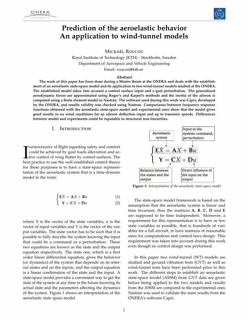
best practice to use the well established control theoryfor these purposes is to have a state-space represen-tation of the aeroelastic system that is a time-domainmodel in the form:
{EX = AX + Bu
Y = CX + Du
(1)
(2)
where X is the vector of the state variables, u is thevector of input variables and Y is the vector of the out-put variables. The state vector has to be such that it ispossible to fully describe the system knowing the inputthat could be a command or a perturbation. Thesetwo equations are known as the state and the outputequation respectively. The state one, which is a firstorder linear differential equation, gives the behavior(or dynamics) of the system that depends on its inter-nal states and on the inputs, and the output equationis a linear combination of the state and the input. Astate-space model provides a convenient way to get thestate of the system at any time in the future knowing itsactual state and the parameters affecting the dynamicsof the system. Figure 1 shows an interpretation of theaeroelastic state space model.
Figure 1: Interpretation of the aeroelastic state-space model
The state-space model framework is based on theassumption that the aeroelastic system is linear andtime invariant, thus the matrices A, B, C, D and Eare supposed to be time independent. Moreover, arequirement for this representation is to have as fewstate variables as possible, that is hundreds of vari-ables for a full aircraft, to have matrices of reasonablesizes for computations and control laws design. Thisrequirement was taken into account during this workeven though no control design was performed.
In this paper two wind-tunnel (WT) models arestudied and ground vibration tests (GVT) as well aswind-tunnel tests have been performed prior to thiswork. The different steps to establish an aeroelasticstate-space model (ASSM) from GVT data are givenbefore being applied to the two models and resultsfrom the ASSM are compared to the experimental ones.Nastran was used to validate the main results from theONERA’s software Capri.
1
II. Wind-tunnel models
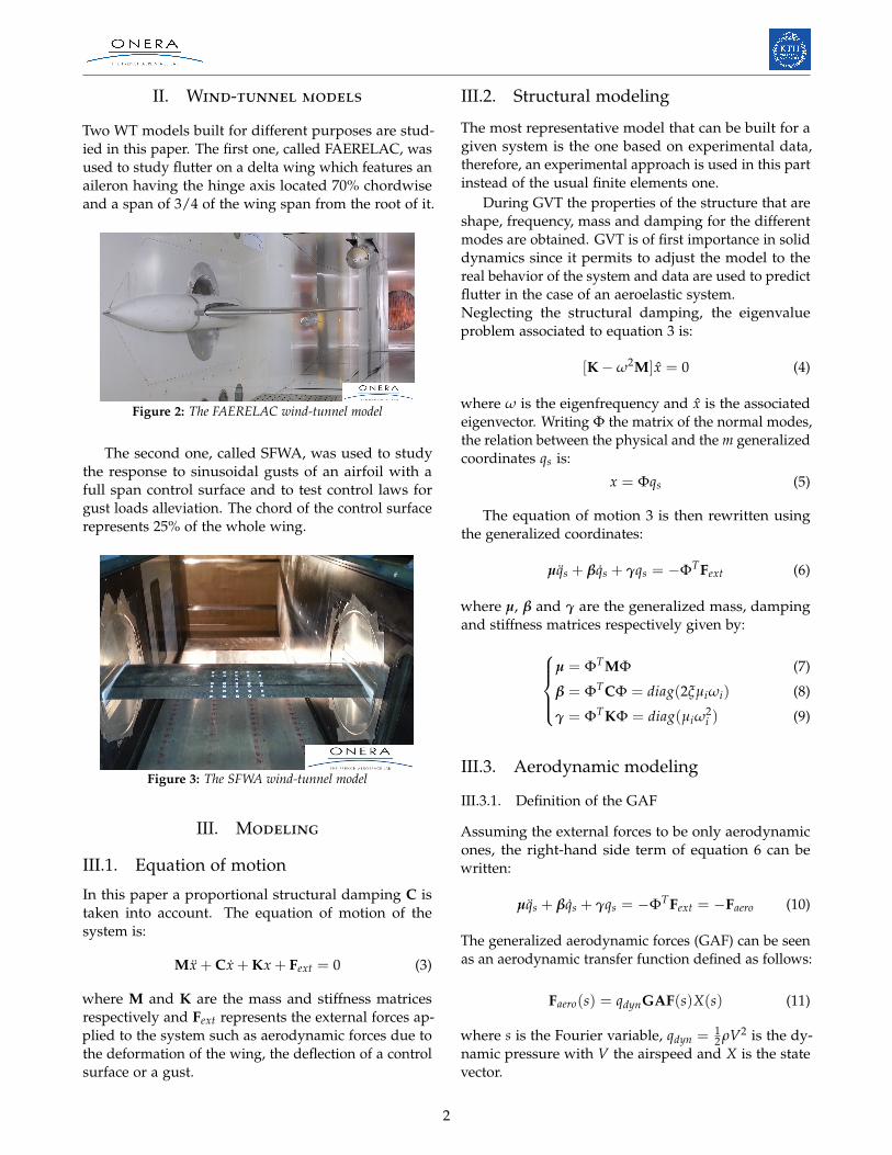
Two WT models built for different purposes are stud-ied in this paper. The first one, called FAERELAC, wasused to study flutter on a delta wing which features anaileron having the hinge axis located 70% chordwiseand a span of 3/4 of the wing span from the root of it.
Figure 2: The FAERELAC wind-tunnel model
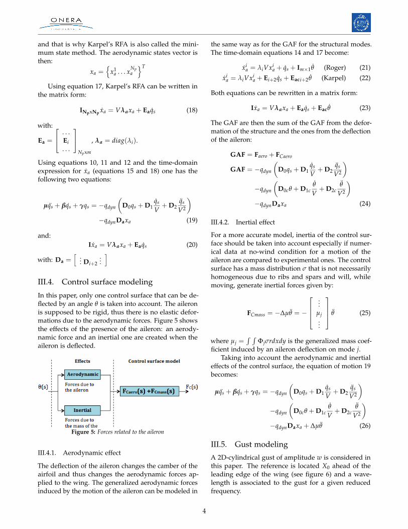
The second one, called SFWA, was used to studythe response to sinusoidal gusts of an airfoil with afull span control surface and to test control laws forgust loads alleviation. The chord of the control surfacerepresents 25% of the whole wing.
Figure 3: The SFWA wind-tunnel model
III. Modeling
III.1. Equation of motion
In this paper a proportional structural damping C istaken into account. The equation of motion of thesystem is:
Mx + Cx + Kx + Fext = 0 (3)
where M and K are the mass and stiffness matricesrespectively and Fext represents the external forces ap-plied to the system such as aerodynamic forces due tothe deformation of the wing, the deflection of a controlsurface or a gust.
III.2. Structural modeling
The most representative model that can be built for agiven system is the one based on experimental data,therefore, an experimental approach is used in this partinstead of the usual finite elements one.
During GVT the properties of the structure that areshape, frequency, mass and damping for the differentmodes are obtained. GVT is of first importance in soliddynamics since it permits to adjust the model to thereal behavior of the system and data are used to predictflutter in the case of an aeroelastic system.Neglecting the structural damping, the eigenvalueproblem associated to equation 3 is:
[K−ω2M]x = 0 (4)
where ω is the eigenfrequency and x is the associatedeigenvector. Writing Φ the matrix of the normal modes,the relation between the physical and the m generalizedcoordinates qs is:
x = Φqs (5)
The equation of motion 3 is then rewritten usingthe generalized coordinates:
µqs + βqs + γqs = −ΦTFext (6)
where µ, β and γ are the generalized mass, dampingand stiffness matrices respectively given by:
µ = ΦTMΦ
β = ΦTCΦ = diag(2ξµiωi)
γ = ΦTKΦ = diag(µiω2i )
(7)
(8)
(9)
III.3. Aerodynamic modeling
III.3.1. Definition of the GAF
Assuming the external forces to be only aerodynamicones, the right-hand side term of equation 6 can bewritten:
µqs + βqs + γqs = −ΦTFext = −Faero (10)
The generalized aerodynamic forces (GAF) can be seenas an aerodynamic transfer function defined as follows:
Faero(s) = qdynGAF(s)X(s) (11)
where s is the Fourier variable, qdyn = 12 ρV2 is the dy-
namic pressure with V the airspeed and X is the statevector.
2

III.3.2. Doublet Lattice Method
The Doublet Lattice Method (DLM) is an efficient andreliable method to derive the unsteady aerodynamicforces. This method was developed in the 60’s and isbased on the linearized potential flow theory and theassumption of harmonic motions of the lifting surfacesthat are approximated as flat plates of infinitesimalthickness. The DLM has the advantage of not being astime-consuming as the field methods but more accu-rate than the strip theory. More details about the DLMcan be found in [1].
With the DLM the aerodynamic forces are com-puted for a specific Mach number and a given reducedfrequency k = ωc
2V where c is the mean chord of thewing and ω = 2π f with f the frequency of the struc-tural oscillations. Therefore one gets the GAF only fora discrete set of points in the frequency domain. Thisis sufficient to perform a flutter analysis with the p-kmethod, as explained in [2], but in order to establishthe ASSM one needs to know the GAF for all points inthe frequency range of interest and thus one needs ananalytic representation of the GAF.
III.3.3. Rational function approximation (RFA)
The main difficulty when establishing an ASSM is tofind a good representation of the GAF in the frequencydomain. A solution is to use a rational function approx-imation (RFA) and although several models were devel-oped, two of them are of best importance: Roger’s andKarpel’s methods which approximate the GAF with acomplex rational function. Figure 4 shows the differentsteps for the aerodynamic modeling.
Figure 4: Aerodynamic modeling
The starting point of these two methods is to con-sider the following form for the GAF in the frequencydomain:
GAF(s) = D0 + D1sV
+ D2s2
V2 +Np
∑i=1
Di+2Pi(s) (12)
The three terms D0, D1 and D2 give the aerodynamicforces as a function of the structural states, with thestatic given by the D0 matrix, but they are not suffi-cient to accurately describe the GAF. Indeed, there isa lag between the motion of the system and the in-duced aerodynamic forces, therefore, lag terms have
to be added to the expression of the GAF to take thisphenomenon into account and that is the role of thesum. The number Np of these terms depends on theaccuracy of the approximation desired while keepingin mind that each additional term introduces aerody-namic states in the ASSM.
The difference between Roger’s and Karpel’s RFAlies on the form of the lag terms that leads to a differentnumber of additional states.
Roger’s RFARoger was the first to approximate the GAF with acomplex rational function. He modeled the lag termsby:
Pi(s) =s/V
s/V − λi(13)
where λi represents the aerodynamic pole of Pi. Thisequation can be seen as a transfer function between theaerodynamic states xi
a that are introduced due to thelag and the vector of the structural states qs and givesin the time domain:
xia = λiVxi
a + qs (14)
Since qs is a column vector of m components, this is asystem of linear first-order differential equations andone can notice that for each introduced aerodynamicpole m aerodynamic states are created. Therefore, as-suming that Np aerodynamic poles are introduced,n = Np×m aerodynamic states are introduced and theaerodynamic states vector is:
xa ={
x1a1
. . . x1am . . . . . . x
Npa1 . . . x
Npam
}T
Using equation 14, Roger’s RFA can be written in thematrix form:
Inxn xa = Vλaxa + Ea qs (15)
with:
Ea =
. . .
Inxm. . .
, λa =
λ1Imxm. . .
λNp Imxm
Karpel’s RFAKarpel used another expression for the lag terms:
Pi(s) =s/V
s/V − λiEi+2 (16)
where Ei+2 is a row vector. In the time-domain, thisgives:
xia = λiVxi
a + Ei+2qs (17)
Unlike equation 14, this is a scalar linear first-orderequation. Thus, with Karpel’s RFA one introduces onlyone aerodynamic states per added aerodynamic pole
3
and that is why Karpel’s RFA is also called the mini-mum state method. The aerodynamic states vector isthen:
xa ={
x1a . . . x
Npa
}T
Using equation 17, Karpel’s RFA can be written inthe matrix form:
INpxNp xa = Vλaxa + Ea qs (18)
with:
Ea =
. . .Ei. . .
Npxm
, λa = diag(λi).
Using equations 10, 11 and 12 and the time-domainexpression for xa (equations 15 and 18) one has thefollowing two equations:
µqs + βqs + γqs = −qdyn
(D0qs + D1
qs
V+ D2
qs
V2
)−qdynDaxa (19)
and:Ixa = Vλaxa + Ea qs (20)
with: Da =[
... Di+2...]
III.4. Control surface modeling
In this paper, only one control surface that can be de-flected by an angle θ is taken into account. The aileronis supposed to be rigid, thus there is no elastic defor-mations due to the aerodynamic forces. Figure 5 showsthe effects of the presence of the aileron: an aerody-namic force and an inertial one are created when theaileron is deflected.
Figure 5: Forces related to the aileron
III.4.1. Aerodynamic effect
The deflection of the aileron changes the camber of theairfoil and thus changes the aerodynamic forces ap-plied to the wing. The generalized aerodynamic forcesinduced by the motion of the aileron can be modeled in
the same way as for the GAF for the structural modes.The time-domain equations 14 and 17 become:
xia = λiVxi
a + qs + Im×1θ (Roger) (21)
xia = λiVxi
a + Ei+2qs + Eac i+2θ (Karpel) (22)
Both equations can be rewritten in a matrix form:
Ixa = Vλaxa + Ea qs + Eac θ (23)
The GAF are then the sum of the GAF from the defor-mation of the structure and the ones from the deflectionof the aileron:
GAF = Faero + FCaero
GAF = −qdyn
(D0qs + D1
qs
V+ D2
qs
V2
)−qdyn
(D0cθ + D1c
θ
V+ D2c
θ
V2
)−qdynDaxa (24)
III.4.2. Inertial effect
For a more accurate model, inertia of the control sur-face should be taken into account especially if numer-ical data at no-wind condition for a motion of theaileron are compared to experimental ones. The controlsurface has a mass distribution σ that is not necessarilyhomogeneous due to ribs and spars and will, whilemoving, generate inertial forces given by:
FCmass = −∆µθ = −
...
µj...
θ (25)
where µj =∫ ∫
Φjσrdxdy is the generalized mass coef-ficient induced by an aileron deflection on mode j.
Taking into account the aerodynamic and inertialeffects of the control surface, the equation of motion 19becomes:
µqs + βqs + γqs = −qdyn
(D0qs + D1
qs
V+ D2
qs
V2
)−qdyn
(D0cθ + D1c
θ
V+ D2c
θ
V2
)−qdynDaxa + ∆µθ (26)
III.5. Gust modeling
A 2D-cylindrical gust of amplitude w is considered inthis paper. The reference is located X0 ahead of theleading edge of the wing (see figure 6) and a wave-length is associated to the gust for a given reducedfrequency.
4
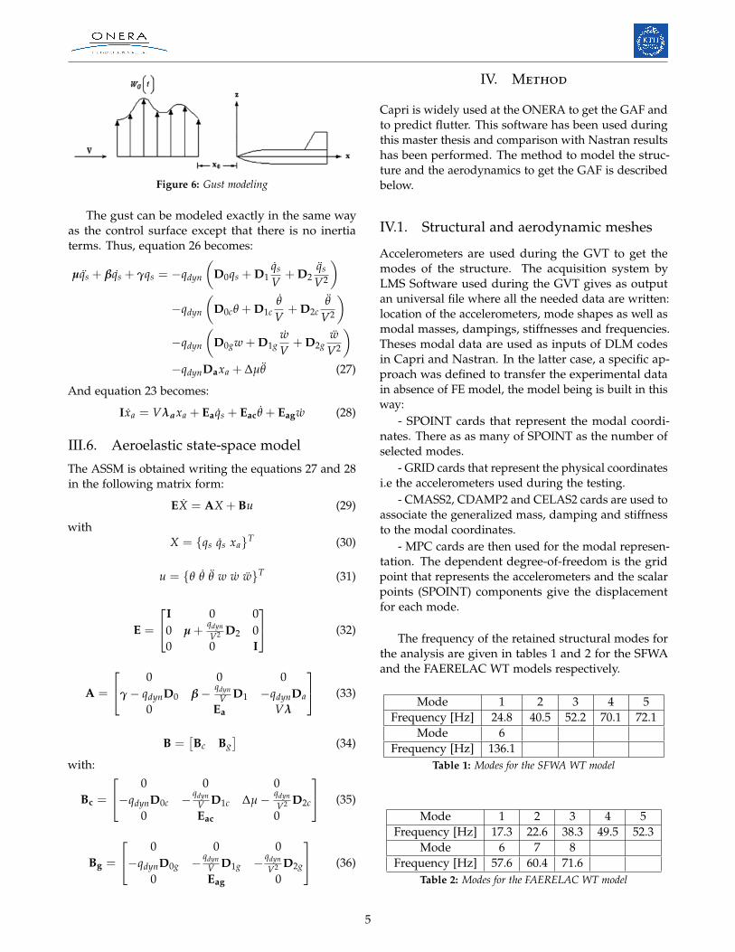
Figure 6: Gust modeling
The gust can be modeled exactly in the same wayas the control surface except that there is no inertiaterms. Thus, equation 26 becomes:
µqs + βqs + γqs = −qdyn
(D0qs + D1
qs
V+ D2
qs
V2
)−qdyn
(D0cθ + D1c
θ
V+ D2c
θ
V2
)−qdyn
(D0gw + D1g
wV
+ D2gwV2
)−qdynDaxa + ∆µθ (27)
And equation 23 becomes:
Ixa = Vλaxa + Ea qs + Eac θ + Eagw (28)
III.6. Aeroelastic state-space model
The ASSM is obtained writing the equations 27 and 28in the following matrix form:
EX = AX + Bu (29)
withX = {qs qs xa}T (30)
u = {θ θ θ w w w}T (31)
E =
I 0 00 µ +
qdynV2 D2 0
0 0 I
(32)
A =
0 0 0γ− qdynD0 β− qdyn
V D1 −qdynDa0 Ea Vλ
(33)
B =[Bc Bg
](34)
with:
Bc =
0 0 0−qdynD0c − qdyn
V D1c ∆µ− qdynV2 D2c
0 Eac 0
(35)
Bg =
0 0 0−qdynD0g − qdyn
V D1g − qdynV2 D2g
0 Eag 0
(36)
IV. Method
Capri is widely used at the ONERA to get the GAF andto predict flutter. This software has been used duringthis master thesis and comparison with Nastran resultshas been performed. The method to model the struc-ture and the aerodynamics to get the GAF is describedbelow.
IV.1. Structural and aerodynamic meshes
Accelerometers are used during the GVT to get themodes of the structure. The acquisition system byLMS Software used during the GVT gives as outputan universal file where all the needed data are written:location of the accelerometers, mode shapes as well asmodal masses, dampings, stiffnesses and frequencies.Theses modal data are used as inputs of DLM codesin Capri and Nastran. In the latter case, a specific ap-proach was defined to transfer the experimental datain absence of FE model, the model being is built in thisway:
- SPOINT cards that represent the modal coordi-nates. There as as many of SPOINT as the number ofselected modes.
- GRID cards that represent the physical coordinatesi.e the accelerometers used during the testing.
- CMASS2, CDAMP2 and CELAS2 cards are used toassociate the generalized mass, damping and stiffnessto the modal coordinates.
- MPC cards are then used for the modal represen-tation. The dependent degree-of-freedom is the gridpoint that represents the accelerometers and the scalarpoints (SPOINT) components give the displacementfor each mode.
The frequency of the retained structural modes forthe analysis are given in tables 1 and 2 for the SFWAand the FAERELAC WT models respectively.
Mode 1 2 3 4 5Frequency [Hz] 24.8 40.5 52.2 70.1 72.1
Mode 6Frequency [Hz] 136.1
Table 1: Modes for the SFWA WT model
Mode 1 2 3 4 5Frequency [Hz] 17.3 22.6 38.3 49.5 52.3
Mode 6 7 8Frequency [Hz] 57.6 60.4 71.6
Table 2: Modes for the FAERELAC WT model
5

The aerodynamic mesh is then created in Capri orNastran keeping in mind that the coordinates systemmust be as follows: the x-axis is chordwise and in thesame direction as the wind, the y-axis is spanwise fromthe root to the tip of the wing and the z-axis is upwards.
Figures 7 and 8 show the structural mesh (the ac-celerometers are represented as points and the ones ofinterest for later are numbered) and the aerodynamicmesh (panels) created in Capri for both wind-tunnelmodels.
x-0.4 -0.2 0 0.2 0.4 0.6 0.8 1 1.2
y
0
0.2
0.4
0.6
0.8
1
Accel. 5
Accel. 14
Accel. 22
Tank
Missile
Figure 7: Structural and aerodynamic meshes, FAERELAC
x
-0.4
-0.3
-0.2
-0.1
0
0.1
0.2
0.3
0.4
0.5
y-0.4 -0.3 -0.2 -0.1 0 0.1 0.2 0.3 0.4
Accel. 8 Accel. 12
Accel. 9
Figure 8: Structural and aerodynamic meshes, SFWA
IV.2. Aileron deflection and gust modeling
To take the aerodynamic forces induced by the ailerondeflection and the gust and prior to the approximationof the GAF, two artificial modes are created for theSFWA WT case and one for the FAERELAC WT case(only aileron input).
IV.3. Coupling
So far the modes are only related to the structuralmesh, thus a coupling between the two meshes mustbe done to transfer the modes on the aerodynamicmesh. With such a coupling, the deformation of thestructure will induce a change in the aerodynamicforces and vice-versa. For both wind-tunnel models
this coupling is done using an infinite plate spline inCapri (INFINITE_PLATE) and in Nastran (SPLINE4).
IV.4. GAF
The Mach numbers, the ranges of reduced frequenciesand the corresponding maximum frequencies for thecomputation of the GAF for the two WT models aregiven table 3. For the modeling to be consistent, it isimportant that the ranges of reduced frequencies con-tains the frequencies of the different modes. The GAFare a direct output of Capri and the ones computedby Nastran are obtained using a DMAP in a SOL145analysis (see [3]).
WT model c Mach kmin kmax fmax[m] [Hz]
SFWA 0.25 0.30 0 1.38 176SFWA 0.25 0.73 0 1.38 423
FAERELAC 0.55 0.70 0 1.38 184Table 3: Mach numbers and reduced frequencies ranges
IV.5. Inertia of the aileron
Depending on the geometry of the aileron (skin thick-ness, ribs, spars) it could be hard to find an analyticalexpression for the mass distribution. The method ap-plied in this paper is to use a finite elements model ofthe aileron since the first step to compute the general-ized inertia forces due to the aileron is to have a dis-cretization of the mass. To do so, a suitable CAD modelof the aileron is imported in Nastran and meshed creat-ing Nnodes nodes. Using a DMAP, the mass mi at eachnode is recovered and the distance ri of it to the aileronhinge axis is computed using its coordinates.This mass discretization is then coupled to the aerody-namic mesh and using the matrix of eigenvectors onegets the inertia terms for mode j:
µj =Nnodes
∑i=1
miriδji (37)
where δji is the amplitude of mode j at the structural
point i.
IV.6. Aileron control and gust transfer func-tions
In the previous section the input u-vector has not onlythe aileron deflection angle and the gust velocity butalso the two first derivatives of these variables whichare not easy to get in practice. Therefore, an extra ef-fort is needed to have one variable per input instead ofthree.
6
IV.6.1. Control modeling
The control system of the wind-tunnel models is com-posed of many elements (a rotative hydraulic actuator,a fast response servo-valve, a rotary variable differ-ential transformer sensor, a conditioning process andfeedback laws) and its dynamics has to be taken intoaccount since it impacts the behavior of the whole con-trol system and especially if it introduces a phase. Inpractice, the input of the control system is not the de-flection angle θ (and thus none of its time-derivatives)but a voltage U. Indeed, the control surface is movedthanks to an actuator that needs a voltage U as inputto deflect the aileron by an angle θ. Using experimentsit is possible to get the Frequency Response Function(FRF) of the control system in order to approximate itsdynamics with a transfer function between the angle θand the input voltage U. as presented in figure 9.
Figure 9: Transfer function G
This system identification can be performed usingthe in-built MATLAB function tfest which is part ofthe System Identification Toolbox. Figures 10 and 11show the experimental FRF for the two wind-tunnelmodels. In both figures, the red line corresponds to theidentified transfer function.
For the SFWA WT model, a second-order transferfunction with cutoff frequency ω0 = 2π ∗ 350 rad/sdamping coefficient ξ = 0.16 gives a good correlationfor the magnitude and the phase in the frequenciesrange of interest [0; 140 Hz] and up to 350 Hz that is2.5 times higher than the maximum frequency of theretained modes (136.1 Hz).
Frequency (Hz)0 50 100 150 200 250 300 350 400 450 500
Am
plitu
de °
/ V
10 -1
100
FRF (Control Surface Deflection/Control Surface Command)
Testing2nd-order model
Frequency (Hz)0 50 100 150 200 250 300 350 400 450 500
Pha
se (
deg)
-250
-200
-150
-100
-50
0
50
Figure 10: Control transfer function for SFWA
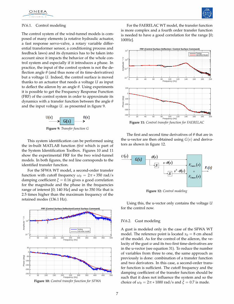
For the FAERELAC WT model, the transfer functionis more complex and a fourth order transfer functionis needed to have a good correlation for the range [0;100Hz].
Frequency (Hz)0 20 40 60 80 100 120 140 160 180 200
Am
plitu
de °
/ V
10 -2
10 -1
100
101 FRF (Control Surface Deflection / Control Surface Command)
TestingIdentified Model
Frequency (Hz)0 20 40 60 80 100 120 140 160 180 200
Pha
se (
deg)
-400
-300
-200
-100
0
100
Figure 11: Control transfer function for FAERELAC
The first and second time derivatives of θ that are inthe u-vector are then obtained using G(s) and deriva-tors as shown in figure 12.
Figure 12: Control modeling
Using this, the u-vector only contains the voltage Ufor the control now.
IV.6.2. Gust modeling
A gust is modeled only in the case of the SFWA WTmodel. The reference point is located x0 = 8 cm aheadof the model. As for the control of the aileron, the ve-locity of the gust w and its two first time-derivatives arein the u-vector (see equation 31). To reduce the numberof variables from three to one, the same approach aspreviously is done: combination of a transfer functionand two derivators. In this case, a second-order trans-fer function is sufficient. The cutoff frequency and thedamping coefficient of the transfer function should besuch that it does not influence the system and so thechoice of ω0 = 2π ∗ 1000 rad/s and ξ = 0.7 is made.
7

V. Results
The ASSM is parametrized with the freestream velocityand the air density so it is possible to perform simula-tions with and without wind. The ones without windcorrespond to the dynamic response of the system to amotion of the aileron.
The developed program during this thesis can takeas input GAF from Capri or Nastran. GAF from Capriand Nastran are very similar (so are the root loci), andthus the validity of Capri is checked and only resultsfrom the ONERA software are presented here.
GAF and root loci obtained using Karpel’s andRoger’s methods are very similar (using 18 poles withKarpel’s and 3 with Roger’s, i.e. 18 introduced aero-dynamic states, for SFWA and 20 poles with Karpel’sand 4 with Roger’s, i.e. 32 introduced aerodynamicstates, for FAERELAC) for both WT models. Thus thedynamics of the modeled system is the same and forthis reason, only FRF obtained with Roger’s RFA arepresented. Regarding root loci, zoom has been done tofocus on the structural modes but the stability of thesystem - that is no poles has a positive real part - hasbeen checked and for clarity, only the four terms of theGAF matrices are presented.
V.1. SFWA wind-tunnel model
The aileron CAD model gives a mass and an inertiaof 0.592 kg and 2.90e-4 kg.m2 and the implementedmethod in Matlab gives 0.592 kg and 2.46e-4 kg.m2.
V.2. Without wind - Aileron command
Figure 13 represents the FRF at the accelerometers 8,9 and 12 on the model (see figure 8) for an aileronexcitation.
Frequency [Hz]20 30 40 50 60 70 80
Am
plitu
de [(
m/s
2)/
V]
10 -2
10 -1
100
101
102 FRF acceleration - Without wind - Aileron command 1 deg
Acc 12 - ExpAcc 9 - ExpAcc 8 - ExpAcc 12 - ASSMAcc 9 - ASSMAcc 8 - ASSM
Frequency [Hz]20 30 40 50 60 70 80
Pha
se [d
eg]
-200
-150
-100
-50
0
50
100
150
200
Figure 13: FRF without wind - Aileron command- SFWA
V.3. Mach 0.30
V.3.1. GAF
The black circles correspond to results from Capri, thered crosses and the blue dots are the ones from theASSM using Karpel’s and Roger’s RFA respectively.
Re(GAFk)
-0.08 -0.06 -0.04 -0.02
Im(G
AF
k)
0
0.01
0.02
0.03
0.04
0.05
0.06
0.07GAF 1,1
Re(GAFk)
-0.16 -0.14 -0.12
Im(G
AF
k)
-0.25
-0.2
-0.15
-0.1
-0.05
0GAF 1,2
Re(GAFk)
0 0.01 0.02 0.03 0.04 0.05Im
(GA
Fk)
0
0.005
0.01
0.015
0.02
0.025
0.03
GAF 2,1
Re(GAFk)
-0.12 -0.1 -0.08 -0.06
Im(G
AF
k)
0
0.05
0.1
0.15
0.2
GAF 2,2
Figure 14: GAF - Mach 0.30 - SFWA
V.3.2. Root locus plot
Squares are the poles from the GVT, black circles arethe poles from Capri, crosses and blue dots are thepoles from the ASSM using Karpel’s and Roger’s RFA.The aspect of the last root locus is due to the lack ofsignificant figures in Capri (beware the scale).
-6 -5.9 -5.8155.3
155.4
155.5
155.6
155.7
155.8
-2.4 -2.2 -2 -1.8
253.8
254
254.2
254.4
254.6
-35.32 -35.31 -35.3 -35.29 -35.28
324
325
326
327
-10.15 -10.1 -10.05 -10440
440.2
440.4
440.6
440.8
-45.2 -45 -44.8 -44.6
448
449
450
451
-4.8 -4.6 -4.4 -4.2
854.6854.7854.8854.9
855855.1
Figure 15: Root locus - Structural modes - Mach 0.30 - SFWA
V.3.3. Frequency response functions (FRF)
The FRF at the accelerometers 8, 9 and 12 for an aileroninput and a gust perturbation are presented in thefigures below.
8

Frequency [Hz]20 30 40 50 60 70 80
Am
plitu
de [(
m/s
2)/
V]
10 -2
100
102 FRF acceleration - Mach 0.30 - Aileron command 1 deg
Acc 12 - ExpAcc 9 - ExpAcc 8 - ExpAcc 12 - ASSMAcc 9 - ASSMAcc 8 - ASSM
Frequency [Hz]20 30 40 50 60 70 80
Pha
se [d
eg]
-200
-150
-100
-50
0
50
100
150
200
Figure 16: FRF aileron command - Mach 0.30 - Roger - SFWA
Frequency [Hz]20 30 40 50 60 70 80
Am
plitu
de [(
m/s
2)/
V]
100
101
FRF acceleration - Mach 0.30 - Gust perturbation
Acc 12 - ExpAcc 9 - ExpAcc 8 - ExpAcc 12 - ASSMAcc 9 - ASSMAcc 8 - ASSM
Frequency [Hz]20 30 40 50 60 70 80
Pha
se [d
eg]
-200
-150
-100
-50
0
50
100
150
200
Figure 17: FRF gust perturbation - Mach 0.30 - Roger - SFWA
V.4. Mach 0.73
V.4.1. GAF
GAF for the pitch and the first flexion modes are givenin the figure below. The circles are the results fromCapri, the crosses and the dots are the ones from theASSM using Karpel’s and Roger’s RFA respectively.
Re(GAFk)
-0.05 0 0.05
Im(G
AF
k)
0
0.05
0.1
0.15
0.2
0.25
0.3
0.35
0.4
GAF 2,2
Re(GAFk)
0 0.01 0.02 0.03 0.04
Im(G
AF
k)
-0.05
-0.04
-0.03
-0.02
-0.01
0GAF 2,4
Re(GAFk)
-0.18 -0.17 -0.16 -0.15 -0.14 -0.13
Im(G
AF
k)
-0.12
-0.1
-0.08
-0.06
-0.04
-0.02
0GAF 4,2
Re(GAFk) #10 -3
-5 0 5
Im(G
AF
k)
0
0.01
0.02
0.03
0.04
0.05
0.06
GAF 4,4
Figure 18: GAF - Mach 0.73 - SFWA
V.4.2. Root locus plot
Squares are the poles from the GVT, circles and crossesare poles from Capri and the ASSM.
-6.8 -6.6 -6.4 -6.2 -6 -5.8
153
154
155
156
-5 -4 -3 -2245
250
255
260
-35.45 -35.4 -35.35 -35.3
323
324
325
326
327
-10.4 -10.3 -10.2 -10.1 -10
439
439.5
440
440.5
441
441.5
-47 -46.5 -46 -45.5 -45 -44.5
440
445
450
455
-6.5 -6 -5.5 -5 -4.5
853
854
855
856
Figure 19: Root locus - Mach 0.73 - SFWA
V.4.3. Frequency response functions (FRF)
The FRF for the accelerometers 8, 9 and 12 obtainedwith Roger’s RFA are represented in the figures below.
Frequency [Hz]20 30 40 50 60 70 80
Am
plitu
de [(
m/s
2)/
V]
100
101
102
FRF acceleration - Mach 0.73 - Aileron command 1 deg
Acc 12 - ExpAcc 9 - ExpAcc 8 - ExpAcc 12 - ASSMAcc 9 - ASSMAcc 8 - ASSM
Frequency [Hz]20 30 40 50 60 70 80
Pha
se [d
eg]
-200
-150
-100
-50
0
50
100
150
200
Figure 20: FRF aileron command - Mach 0.73 - Roger - SFWA
Frequency [Hz]20 30 40 50 60 70 80
Am
plitu
de [(
m/s
2)/
V]
100
101
102
FRF acceleration - Mach 0.73 - Gust perturbation
Acc 12 - ExpAcc 9 - ExpAcc 8 - ExpAcc 12 - ASSMAcc 9 - ASSMAcc 8 - ASSM
Frequency [Hz]20 30 40 50 60 70 80
Pha
se [d
eg]
-200
-150
-100
-50
0
50
100
150
200
Figure 21: FRF gust perturbation - Mach 0.73 - Roger - SFWA
9
V.5. FAERELAC wind-tunnel model
The CAD model of the aileron gives a mass and an iner-tia of 4.406 kg and 3.02e-2 kg.m2 and the implementedmethod in Matlab gives 4.2 kg and 2.88e-2 kg.m2.
V.6. Without wind - Aileron command
The FRF at for the three accelerometers shown in figure7 for an aileron command are given below.
Frequency [Hz]20 30 40 50 60 70 80 90 100
Am
plitu
de [(
m/s
2)/
V]
10 -2
100
102
FRF acceleration - Without wind - Aileron command
Accel 5 - ExpAccel 14 - ExpAccel 22 - ExpAccel 5 - ASSMAccel 14 - ASSMAccel 22 - ASSM
Frequency [Hz]20 30 40 50 60 70 80 90 100
Pha
se [d
eg]
-400
-300
-200
-100
0
100
200
300
Figure 22: FRF without wind - Aileron command- FAERELAC
V.7. Mach 0.70
V.7.1. GAF
The black circles correspond to results from Capri, thered crosses and the blue dots are the ones from theASSM using Karpel’s and Roger’s RFA respectively(beware the scale).
Re(GAFk)
0.06 0.08 0.1 0.12 0.14
Im(G
AF
k)
0
0.1
0.2
0.3
0.4
0.5
GAF 1,1
Re(GAFk)
-0.6 -0.5 -0.4 -0.3
Im(G
AF
k)
-0.25
-0.2
-0.15
-0.1
-0.05
0GAF 1,2
Re(GAFk)
0.15 0.16 0.17 0.18
Im(G
AF
k)
#10 -3
-5
0
5
10
15
20GAF 2,1
Re(GAFk)
-0.35 -0.3 -0.25
Im(G
AF
k)
0
0.1
0.2
0.3
0.4
0.5
GAF 2,2
Figure 23: GAF - Mach 0.70 - FAERELAC
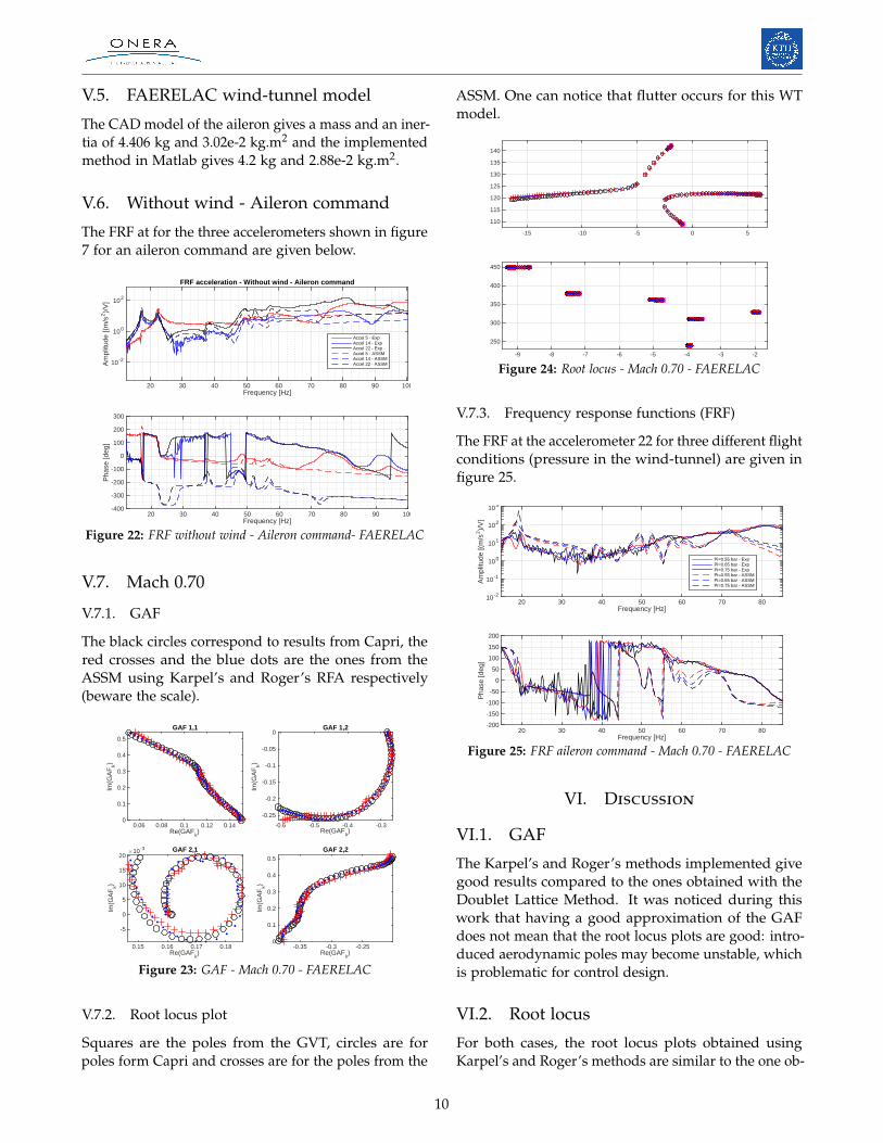
V.7.2. Root locus plot
Squares are the poles from the GVT, circles are forpoles form Capri and crosses are for the poles from the
ASSM. One can notice that flutter occurs for this WTmodel.
-15 -10 -5 0 5
110
115
120
125
130
135
140
-9 -8 -7 -6 -5 -4 -3 -2
250
300
350
400
450
Figure 24: Root locus - Mach 0.70 - FAERELAC
V.7.3. Frequency response functions (FRF)
The FRF at the accelerometer 22 for three different flightconditions (pressure in the wind-tunnel) are given infigure 25.
Frequency [Hz]20 30 40 50 60 70 80
Am
plitu
de [(
m/s
2)/
V]
10 -2
10 -1
100
101
102
103 FRF acceleration - Mach 0.7 - Aileron command - Pi = 0.55, 0.65 and 0.75
Pi=0.55 bar - ExpPi=0.65 bar - ExpPi=0.75 bar - ExpPi=0.55 bar - ASSMPi=0.65 bar - ASSMPi=0.75 bar - ASSM
Frequency [Hz]20 30 40 50 60 70 80
Pha
se [d
eg]
-200
-150
-100
-50
0
50
100
150
200
Figure 25: FRF aileron command - Mach 0.70 - FAERELAC
VI. Discussion
VI.1. GAF
The Karpel’s and Roger’s methods implemented givegood results compared to the ones obtained with theDoublet Lattice Method. It was noticed during thiswork that having a good approximation of the GAFdoes not mean that the root locus plots are good: intro-duced aerodynamic poles may become unstable, whichis problematic for control design.
VI.2. Root locus
For both cases, the root locus plots obtained usingKarpel’s and Roger’s methods are similar to the one ob-
10

tained with the p-k method, and both methods predictthe same flutter speed for the FAERELAC wind-tunnelmodel. Since a root locus plot shows the behavior ofthe aeroelastic system (static divergence, flutter, cou-pling between modes, ...) it is important that the oneobtained from the ASSM is checked and comparedto the root locus plot obtained with the p-k methodbefore performing simulation. Indeed, the number ofpoles and the type of them (real or complex) chosen forthe rational function approximation of the GAF play abig part in the stability of the state-space model. Forinstance, for the SFWA wind-tunnel model the ASSMis stable when approximating the GAF using Roger’smethod with three complex poles but is unstable withfour poles: an aerodynamic one goes from a negativereal part to a positive one.
VI.3. FRF
When comparing the FRF from the ASSM and the onesfrom the experiments, one can say that the correla-tion is good for both amplitude and phase in no windcondition for the two WT models. Moreover, resultsat high frequencies could be improved taking into ac-count residuals in the model. These results allow usto think that this model could be used during GVT topredict the modal behavior of the structure using anaileron excitation instead of the usual shakers.
VI.3.1. SFWA
The experimental set-up used to provide the two de-gree of freedom (heave and pitch) introduced non-linear effects in the system. Since the ASSM is based onlinearity hypothesis, it does not capture structural non-linear effects. When looking at the FRF without wind,one can note that the first mode (heave) around 25 Hzis not visible in the experimental results. This is dueto the non-linear effects at the boundaries that preventthe structure to be excited at this mode. This can alsobe seen for the second mode in the experimental FRFand especially at Mach 0.73 for an aileron command:the mode is not symmetric around the mode frequency.When comparing the FRF in the case of a gust pertur-bation for both Mach numbers, a big difference can benoticed for the second mode (pitch). During the wind-tunnel testing, this mode could not be properly exciteddue to strong friction phenomena. These non-lineareffects introduce differences regarding the phase whichcould be a problem when designing control laws.
The main purpose of this WT model being gustloads alleviation, one would want to dispose of anASSM close to the experiments for a gust perturbation.Basically, to reproduce the absence of the pitch mode
contribution, the modal damping can was artificiallyincreased. Results at Mach 0.73 for these this methodis given below.
Frequency [Hz]20 30 40 50 60 70 80
Am
plitu
de [(
m/s
2)/
V]
101
102
FRF acceleration - Mach 0.73 - Gust perturbation - Damp. mode 2: 0.3
Acc 12 - ExpAcc 9 - ExpAcc 8 - ExpAcc 12 - ASSMAcc 9 - ASSMAcc 8 - ASSM
Frequency [Hz]20 30 40 50 60 70 80
Pha
se [d
eg]
-200
-150
-100
-50
0
50
100
150
200
Figure 26: FRF gust perturbation - Mach 0.73 - Roger - SFWA
VI.3.2. FAERELAC
The comparison at Mach 0.7 is disappointing, espe-cially for the two first modes. The reasons for this arestill under investigation (shocks, flow separation onthe wing, experimental procedures,...).
Conclusion
During this master thesis at the ONERA, an aeroelasticstate-space model that takes into account a control sur-face and a gust perturbation was established using theKarpel’s and Roger’s rational function approximationsfor the generalized aerodynamic forces. The approachwas then applied to two wind-tunnel models and theresults are convincing in no-wind conditions. Dueto structural non-linearities for these two models, theresults in the wind are less accurate but could be im-proved by taking into account residuals or uncertaintieson the modal properties such as frequency or damping.
I would like to thank D. Eller for accepting to bemy KTH supervisor and the whole DADS/ADSE teamfor the great atmosphere during my master thesis andespecially P. Naudin head of the unit, A. Lepage myONERA supervisor and D. Le Bihan for sharing hisexperience.
References
[1] E. Albano and W.P. Roden. A doublet-lattice methodfor calculating lift distributions on oscillating surfaces
11

in subsonic flows. AIAA Journal, vol. 7, issue 2, pp.279-285, 1969
[2] Dan Borglund and David Eller. Aeroelasticity ofSlender Wing Structures in Low-Speed Airflow. Lec-
ture Notes, KTH Aeronautical and Vehicle Engi-neering, 2010
[3] Anthony S. Potozky. Enhanced Modeling of First-Order Plant Equations of Motion for Aeroelastic andAeroservoelastic applications. Paper, AIAA, 2010
12