Computers & Fluids 106 (2015) 67–78

Contents lists available at ScienceDirect

Computers & Fluids

journal homepage: www.elsevier .com/ locate /compfluid

Prediction of the unsteady turbulent flow in an axial compressor stage.Part 2: Analysis of unsteady RANS and LES data

http://dx.doi.org/10.1016/j.compfluid.2014.09.0440045-7930/� 2014 Elsevier Ltd. All rights reserved.

⇑ Address: ISAE, Dpt. of Aerodynamics, Energetics and Propulsion, 10 av. EdouardBelin, Toulouse, France. Tel.: +33 561339255.

E-mail address: Nicolas.Gourdain@isae.fr

1 The estimation of this level of roughness is based on the criterion ks <

with ks the size of roughness and C the blade chord [4].

Nicolas Gourdain ⇑CERFACS, Computational Fluid Dynamics Team, Toulouse, FranceISAE, Dpt. of Aerodynamics, Energetics and Propulsion, 10 av. Edouard Belin, Toulouse, France

a r t i c l e i n f o a b s t r a c t

Article history:Received 15 September 2013Received in revised form 3 September 2014Accepted 30 September 2014Available online 12 October 2014

Keywords:Large-Eddy SimulationRANSRotor/stator interactionsLaminar-to-turbulent transition

This paper presents the analysis of URANS and LES database in a stage of an axial subsonic compressor.Details about numerical methods and comparison with experiments can be found in a companion paper.The analysis here focuses on the transition processes that take place in the rotor and stator rows. In therotor, LES and URANS show that transition develops at mid-chord and is induced by the adverse pressuregradient. In the stator, the flow behavior is more complex since the transition is influenced by the rotorpassing wakes, a laminar separation bubble on the suction side and the accumulation of rotor wakes onthe pressure side. The analysis also investigates the unsteady flow patterns at the rotor/stator interface,from mid-span to the casing. In the tip region, LES shows the development of frequencies that are notcorrelated to the blade passing frequency, while URANS only predicts multiples of the blade passingfrequency.

� 2014 Elsevier Ltd. All rights reserved.

1. Introduction

The maximization of turbomachinery component efficiencyrelies on the capabilities of designers to better account forunsteady flow effects. Among these unsteady flows, two categoriesare of primary interest: rotor/stator interactions, which are peri-odic in time, and turbulence which is an non periodic phenome-non. As reported by Jahanmiri [12], ‘‘the (turbomachinery) flow isa veritable-fluid-dynamical zoo, characterized by separation, reat-tachment, transition, relaminarization, retransition, etc. all oftenoccurring in the same flow’’. The flow behavior becomes particu-larly complex when considering a stage of a turbomachine (forinstance a rotor followed by a stator) operating at industrial-rele-vant conditions (high Reynolds number, compressible flow, etc.).These flows have a strong influence on the state of boundary layers(transition), which is of paramount importance to predict the glo-bal performance of a turbomachine in [31].

There are some indications in the literature that the effects ofsurface curvature, divergence/convergence effects, compressibility,and heat transfer in gas turbines are less significant on transition ascompared to free-stream turbulence effects [12]. Previous worksalso reports that transition [4] as well as the level of losses [4,1]

is sensitive to surface roughness. However, since the Reynoldsnumber related to the test case considered in this paper is quitehigh (Re ¼ 7� 105), a low level of roughness (< 11 lm) 1 shouldnot influence the near wall flow. Indeed, transition in the presentcompressor should be controlled mainly by the free-stream turbu-lence, pressure gradient and periodic incoming wakes.

Despite some interesting works [11], measurements for transi-tional flow under real operating conditions (strong acceleratingflows, high-freestream turbulence, relaminarization, etc.) remainssparse [12]. Indeed, for this purpose CFD is considered more andmore frequently as complementary to experimental campaigns.Different methods to compute unsteady flows have been testedin the literature to study transition phenomena in turbomachinery,such as URANS, LES and DNS [24,29]. While unsteady RANS usuallyprovides a fair reproduction of the periodic unsteady flows, it onlyreproduces partially the flow pattern details observed by DNS andLES, especially for the wake dynamics and on the blade suction side[24].

The increase of the computational capability allows nowadaysthe handling of LES at high Reynolds numbers (Re � 106), in com-plex geometries representative of industrial configurations[31,32,3,9,20]. Indeed, LES appears as a very promising way tostudy transitional flows in turbomachinery components and brings

100Re � C,

Nomenclature

LatinC blade chordh radial heightH compressor vein heightk turbulent kinetic energyM Mach numberM0;1;2 type of grid (see Table 2)n normal to the wall componentp pressureQ mass flowr radial component/directionRe Reynolds numbers streamwise componentS curvilinear abscissa or entropySij strain rate tensorT temperatureTu turbulent intensity

ffiffiffiffiffiffiffiffiffiW 0

i2

q=kWk

� �W velocity component (relative frame)x axial direction

Greek, symbols and acronymsd boundary layer thicknessg efficiencygK Kolmogorov length scale� dissipations stress tensorp total-to-total pressure ratiom kinematic viscosityh azimuthal direction, momentum thicknessx compressor rotation speed:SGS sub-grid scale:0 inlet value:2 outlet value:þ normalized value at the walle: resolved fieldBPF blade passing frequencyLES Large-Eddy SimulationRANS Reynolds averaged Navier–StokesRMS Root mean square quantity

Table 1Number of points per blade passage and total for the whole configuration.

Rotor Stator Whole domain

URANS (grid M0) 1:99� 106 1:69� 106 12:72� 106

LES (grid M2) 126:83� 106 107:55� 106 857:28� 106

68 N. Gourdain / Computers & Fluids 106 (2015) 67–78

new insights on the flow physics that take place in these machines[23].

This paper proposes thus to compare the results obtained withURANS and LES in an axial compressor stage. For both approaches,the geometry takes into account the whole 3D flow. Data are ana-lyzed at nominal operating conditions with a particular emphasison the near wall flow, both in rotor and stator parts. The paper isorganized in five sections. In the first one, a summary of the com-pressor test case is presented along with the numerical method.The second section proposes an analysis of the main flow features,through 2D time-averaged and instantaneous flow fields. The thirdsection deals with the analysis of the near wall flow and focuses onthe state of boundary layers through the estimation of turbulentkinetic energy and momentum thickness. The fourth sectionreports an analysis of the flow at the rotor/stator interface, withthe objective to highlight the interactions between rotor and statorparts. The last section proposes an analysis of the transitionmechanisms that take place in the stator vane.

2. Numerical method and test case

A short summary of the test case and numerical method is pro-vided below. More information about the method can be found inthe companion paper [7].

The test case considered for this study is the CME2 compressor,originally investigated at the LEMFI laboratory [6,25]. This is a sin-gle-stage machine with a 30-blades rotor and a 40-vanes stator.The outer tip radius is 0:275 m and the nominal rotation speed is6330� 14 rpm (i.e. f BPF ¼ 3165 Hz). At this rotation speed, themean Reynolds number based on rotor chord and rotor exit veloc-ity is 700,000. At the nominal operating point, the mass flow Q is10:50� 0:1 kg/s, the total-to-total pressure ratio p is 1.15 andthe isentropic efficiency g is 0.92.

Both LES and URANS equations are solved using the CFD codeelsA. This software uses a cell centered approach on structuredmultiblock meshes. More information about the flow solver canbe found in [5] for modeling capabilities and in [8] for High-Perfor-mance Computing capabilities. For both URANS and LES, convec-tive fluxes are computed with a third-order upwind scheme [27].Diffusive fluxes are computed with a second-order centeredscheme. The turbulent viscosity mt is estimated with the two

equations model of Menter [21] based on a k—x formulation. Tran-sition effects are modeled using two transport equations for theintermittency factor c and the Reynolds number based on the tran-sition momentum thickness Reh;t [22,16,2]. For LES, the subgridscale model is the Wall-Adapting Local Eddy-Viscosity (WALE)model [26].

The time-marching is ensured by a second order Dual TimeStepping method [13], which relies on an implicit scheme (witha scalar Lower–Upper Symmetric Successive Over-Relaxation -LU-SSOR- method [33]). The time step is adapted to the mesh res-olution at walls: for URANS, Dtþ ¼ Dt � f BPF is set to 0.0025 (i.e. 400time steps per blade passing period, which is sufficient to providetime step independent results [30]) and for LES Dtþ ¼ 0:00125 (i.e.800 time steps per blade passing period).

The numerical domain consists of three rotor blades and fourstator vanes, in order to respect the natural compressor periodicity.For both URANS and LES, the mesh represents the whole 3Ddomain, including the tip gap. The number of points correspondingto URANS and LES grids are reported in Table 1. The LES grid (M2)corresponds to the finest grid presented in the companion paper,which ensures that mesh criteria recommended in the literature[28,18] to run wall-resolved LES in academic test cases are satisfied(50 < Dsþ < 150; nþ < 1 and 15 < rþ < 40).

3. Analysis of time-averaged and instantaneous flow fields

URANS and LES time-averaged flow fields, shaded with entropy,are plot in Fig. 1 at h=H ¼ 80% (since the walls are considered asadiabatic, entropy can be used as an indicator of the level of losses).The fields show losses on the stator pressure side and in the rotorwake region. The increase of entropy production along the statorpressure side can result either in a separation of the boundary layeror in a transport of entropy contained in the wakes preferentially

Fig. 1. Time-averaged flow field shaded with entropy S at nominal operating conditions, at h=H ¼ 80%: (a) LES and (b) URANS. [J/kg K]. The dashed box shows the location oflosses induced by the tip leakage flow.

N. Gourdain / Computers & Fluids 106 (2015) 67–78 69

on the pressure side. An overview of the skin friction coefficient isshown in Fig. 2. There is no evidence of a boundary layer separa-tion on the stator pressure side. So it confirms that the entropyaccumulation on the stator pressure side is related to the accumu-lation of incoming rotor wakes that preferentially migrate towardsthe stator pressure side. Both LES and URANS show this effect.However, the wakes predicted with URANS are thicker than thosepredicted by LES and are associated to a higher level of entropy.

The dashed box in Fig. 1 underlines the location of the lossesinduced by the tip leakage flow. In the case of LES, this region startsclose to the rotor trailing edge and is concentrated in the rotorwake region. In the case of URANS, the influence of the tip leakageflow starts at mid-distance between the rotor and the stator, and itspreads in the whole rotor passage.

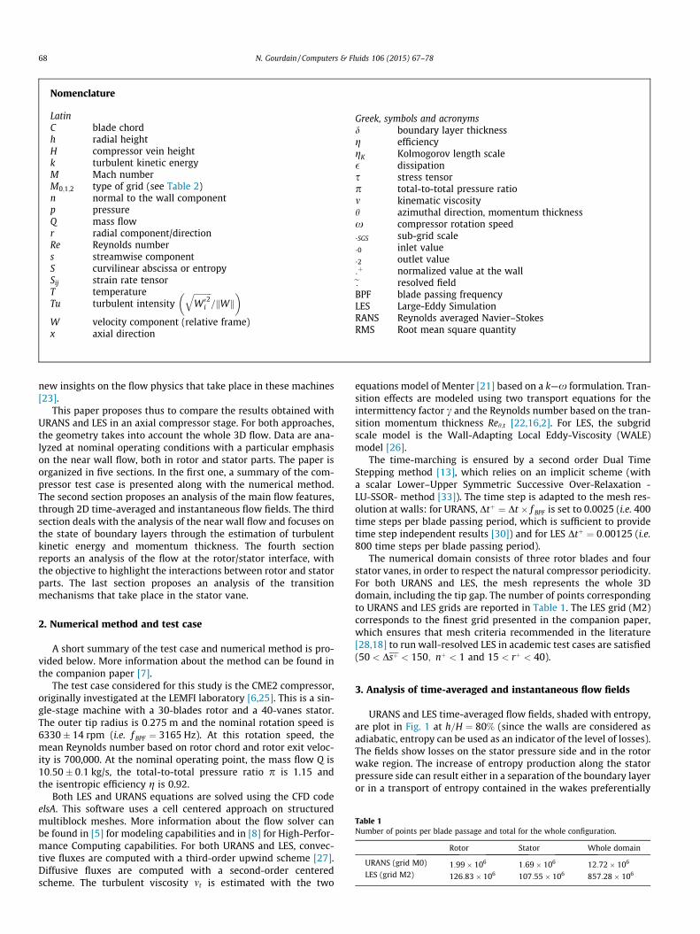
This observation is confirmed in Figs. 3 and 4, which showinstantaneous flow fields, shaded with entropy at two axial posi-tions (rotor/stator interface, x ¼ 75 mm, and downstream the sta-tor, x ¼ 194 mm). At the rotor/stator interface, the azimutalextension of the tip leakage flow as predicted by URANS is moreimportant than with LES. On the URANS flow field, the highentropy region extends from the blade suction side (where thetip leakage emerges) to the next rotor blade pressure side. Onthe LES flow field, the high losses region is restricted to the area

Fig. 2. Time-averaged skin friction coefficient, Cf ¼ 2 � swall=qðxRÞ2tip , from L

close to the rotor suction side and it extends only on half of therotor passage in the azimuthal direction. At the stator exit, Fig. 4,shows that rotor wakes interacts with stator wakes even far fromthe stator trailing edge. This interaction is more visible in the caseof LES, mainly because the rotor wakes are less quickly dissipatedthan with URANS. Downstream the stator, both URANS and LESpredicts a high-entropy region on the last 40% of the compressorspan, due to a boundary layer separation on the stator suction side(zone 2), induced by the high incidence associated to the rotor tipleakage flow. This separation is also observed during the experi-mental campaign [25]. In the pressure side/casing corner, the highentropy region is related to the accumulation of rotor wakes on thestator pressure side (zone 1).

This qualitative analysis shows that LES and URANS predictssimilar flow patterns. However, URANS predicts higher losses thanLES, mainly because URANS shows thicker and deeper rotor wakesthat propagate downstream.

4. Analysis of the near wall flow

The time-averaged wall static pressure is plot in Fig. 5, at mid-span (h=H ¼ 50%). URANS and LES are in good agreement on thesuction side of the rotor and only small differences are observed

ES data at mid-span (h=H ¼ 50%): (a) rotor blade and (b) stator vane.

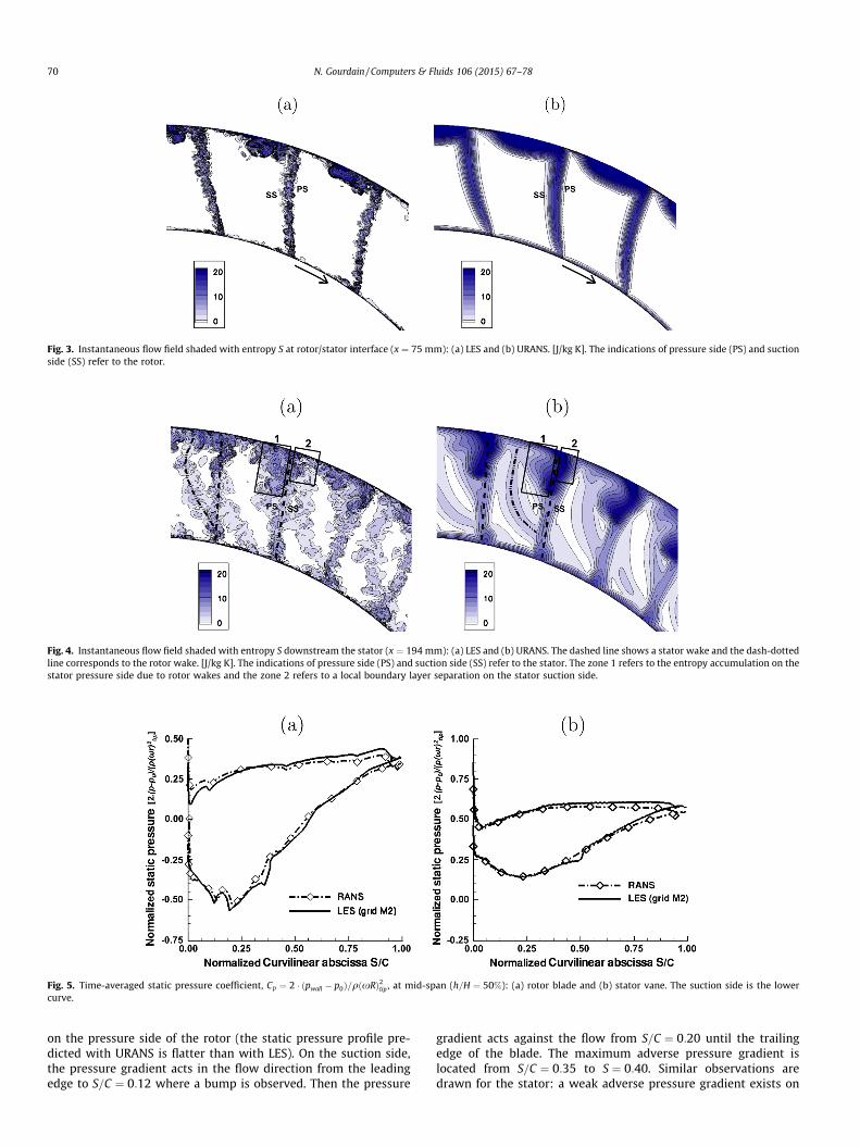
Fig. 3. Instantaneous flow field shaded with entropy S at rotor/stator interface (x ¼ 75 mm): (a) LES and (b) URANS. [J/kg K]. The indications of pressure side (PS) and suctionside (SS) refer to the rotor.

Fig. 4. Instantaneous flow field shaded with entropy S downstream the stator (x ¼ 194 mm): (a) LES and (b) URANS. The dashed line shows a stator wake and the dash-dottedline corresponds to the rotor wake. [J/kg K]. The indications of pressure side (PS) and suction side (SS) refer to the stator. The zone 1 refers to the entropy accumulation on thestator pressure side due to rotor wakes and the zone 2 refers to a local boundary layer separation on the stator suction side.

Fig. 5. Time-averaged static pressure coefficient, Cp ¼ 2 � ðpwall � p0Þ=qðxRÞ2tip , at mid-span (h=H ¼ 50%): (a) rotor blade and (b) stator vane. The suction side is the lowercurve.

70 N. Gourdain / Computers & Fluids 106 (2015) 67–78

on the pressure side of the rotor (the static pressure profile pre-dicted with URANS is flatter than with LES). On the suction side,the pressure gradient acts in the flow direction from the leadingedge to S=C ¼ 0:12 where a bump is observed. Then the pressure

gradient acts against the flow from S=C ¼ 0:20 until the trailingedge of the blade. The maximum adverse pressure gradient islocated from S=C ¼ 0:35 to S ¼ 0:40. Similar observations aredrawn for the stator: a weak adverse pressure gradient exists on

N. Gourdain / Computers & Fluids 106 (2015) 67–78 71

the pressure side from S=C ¼ 0 to S=C ¼ 0:35. On the suction side ofthe stator, the pressure gradient is favorable from S=C ¼ 0 toS=C ¼ 0:25 and it becomes unfavorable on the rest of the chord.LES also predict a steep increase of the pressure gradient on thesuction side of the stator, at S=C ¼ 0:50, compliant with a laminarseparation bubble [14].

The pressure gradient has an effect on the state of boundarylayer, as shown on the production of time-averaged turbulentkinetic energy k, Fig. 6. On the rotor suction side, both LES andURANS predict the onset of transition at S=C ¼ 0:40. On the rotorpressure side, LES shows it at S=C ¼ 0:55 and URANS shows it atS=C ¼ 0:25. Such an early transition of the boundary layer withURANS compared to LES has already been reported in the literature[24]. In the case of LES, the transition is located in the region wherethe adverse pressure gradient is maximum (see Fig. 5). The produc-tion of turbulent kinetic energy k is moderate and quasi-linear onthe pressure side from S=C ¼ 0:50 until the trailing edge(kmax=ðxrÞ2tip ¼ 0:005) compared to the rapid growth on the suctionside from S=C ¼ 0:40 to S=C ¼ 0:45 mm where it reacheskmax=ðxrÞ2tip ¼ 0:020. In the case of URANS, the production of k islower than LES at the transition point on the suction side(kmax=ðxrÞ2tip ¼ 0:010) but the decrease of k follows the sametendency.

In the stator, LES predicts a similar behavior compared to therotor one, except that a small peak of k is observed at the leadingedge due to the incoming rotor wakes (kmax=ðxrÞ2tip ¼ 0:002). Thenthe turbulent kinetic energy vanishes on the suction side untilS=C ¼ 0:50, where transition is observed, kmax=ðxrÞ2tip ¼ 0:011 (thislocation corresponds to the point where the adverse pressure gra-dient is maximum). On the stator pressure side, k reaches its max-imum at S=C ¼ 0:35 (kmax=ðxrÞ2tip ¼ 0:005). The transition point isfound closer to the leading edge on the stator pressure side thanon the suction side, mainly due to the accumulation of high turbu-lent activity contained in the rotor wakes that migrates preferen-tially on the pressure side. The analysis of URANS results show adifferent behavior: the transition spreads on the suction side fromS=C ¼ 0 to S=C ¼ 0:50 and on the pressure side from S=C ¼ 0 toS=C ¼ 0:25.

Actually, the influence of transition on boundary layers can beobserved on the estimation of the Reynolds number based on themomentum thickness, defined as

ReH ¼q1 �Ws;1 �H

l1; ð1Þ

Fig. 6. Evolution of the time-averaged turbulent kinetic energy at mid-span (h=H ¼ 50%)and (b) stator vane.

with H the momentum thickness, as

H ¼Z þ1

0

qWs

ðqWsÞ11� Ws

Ws;1

� �dn: ð2Þ

The estimation of the values outside the boundary layer is nottrivial for the streamwise component of the velocity Ws;1, the den-sity q1 and the viscosity l1. First it depends on the chord locationand then the velocity in the direction normal to the wall does notreach a constant value. The choice has been made to estimate thesevalues by seeking for the maximum in the range 0 < n=d < 1:50.The evolution of ReH based on these estimations is plot in Fig. 7.

In the laminar part of the boundary layers, both LES and URANSpredict the same value for ReH. However, on the pressure side ofthe rotor, since transition starts earlier in the URANS simulation(S=C ¼ 0:25) than in the LES case (S=C ¼ 0:50), the value of ReH

increases more rapidly. As shown in Table 2, at 80% of the rotorchord, the difference on ReH is 83%. The same observation can bedone on the rotor suction side but since both URANS and LES findthe transition at the same location, the difference is lower at thetrailing edge (+31%).

The analysis is completed by a comparison of the time averagedvalue of the velocity fluctuations W 02

i , in the boundary layer of therotor suction side, at S=C ¼ 80%. All values are normalized with thestreamwise velocity outside the boundary layer W2

S;1.As shown in Fig. 8, LES show an anisotropic behavior of the

turbulent fluctuations: W 02x max ¼ 2:2�W 02

h max ¼ 1:6�W 02r max ¼

0:016�W 02S 1, while URANS finds W 02

x max ¼W 02h max ¼W 02

r max ¼0:0075�W 02

S 1. However, errors partially compensate, so URANSpredicts a time-averaged turbulent kinetic energy lower by only32% compared to LES.

URANS predicts the peak of turbulent kinetic energy productionfar to the wall, at n=d ¼ 0:25, compared to LES where the maximumvalue for all velocity components is found below n=d ¼ 0:07. Thecombination ‘‘lower production of turbulent kinetic energy + shiftof the maximum production point away from the wall’’ explainsthe higher sensitivity of the URANS boundary layer to the pressuregradient. This behavior explains the overprediction of the wakedepth and thickness in URANS compared to LES and experiments(see the companion paper).

The quality of LES results can also be estimated a posteriori bycomparing the resolved turbulence gW 02

i (versus) the modeled oneW 02

i SGS, approximated as

, inside the boundary layer at a wall distance of 100 lm (n=d � 0:03): (a) rotor blade

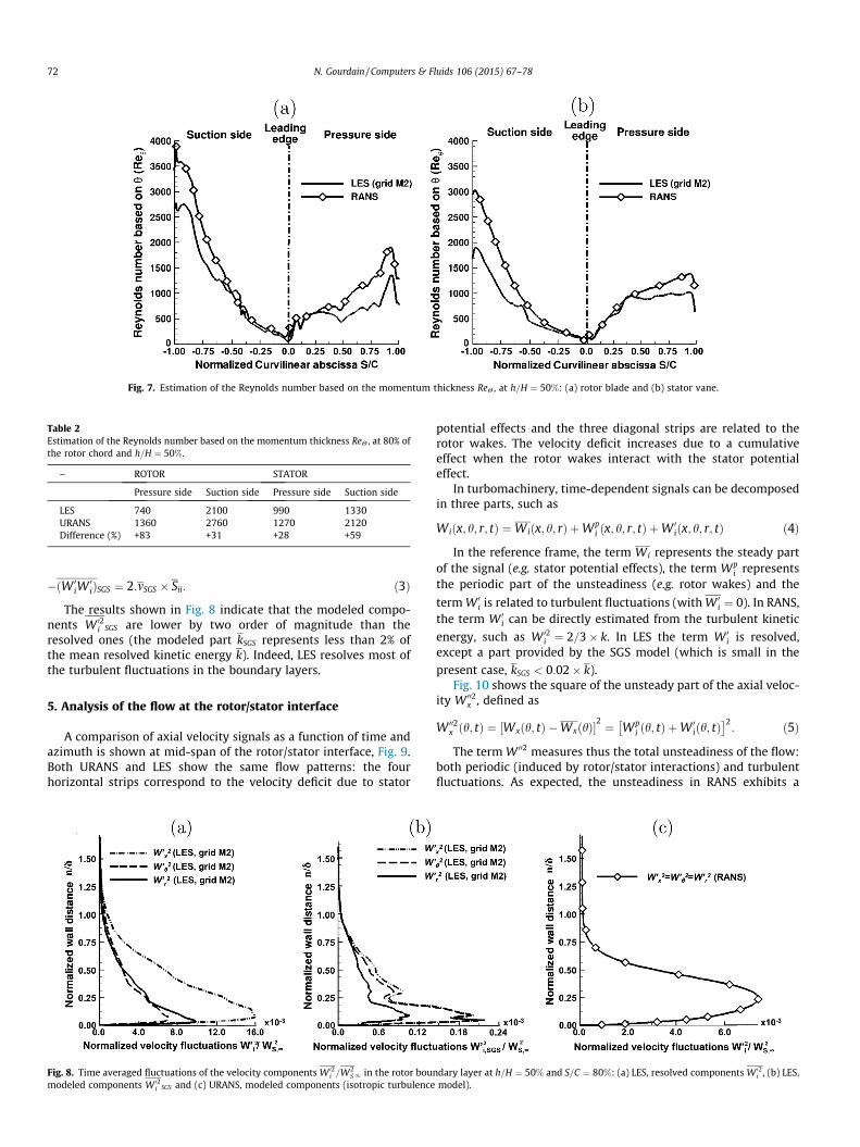
Fig. 7. Estimation of the Reynolds number based on the momentum thickness ReH , at h=H ¼ 50%: (a) rotor blade and (b) stator vane.

Table 2Estimation of the Reynolds number based on the momentum thickness ReH , at 80% ofthe rotor chord and h=H ¼ 50%.

– ROTOR STATOR

Pressure side Suction side Pressure side Suction side

LES 740 2100 990 1330URANS 1360 2760 1270 2120Difference (%) +83 +31 +28 +59

72 N. Gourdain / Computers & Fluids 106 (2015) 67–78

�ðW 0iW

0iÞSGS ¼ 2:mSGS � Sii: ð3Þ

The results shown in Fig. 8 indicate that the modeled compo-nents W 02

i SGS are lower by two order of magnitude than theresolved ones (the modeled part kSGS represents less than 2% ofthe mean resolved kinetic energy k). Indeed, LES resolves most ofthe turbulent fluctuations in the boundary layers.

5. Analysis of the flow at the rotor/stator interface

A comparison of axial velocity signals as a function of time andazimuth is shown at mid-span of the rotor/stator interface, Fig. 9.Both URANS and LES show the same flow patterns: the fourhorizontal strips correspond to the velocity deficit due to stator

Fig. 8. Time averaged fluctuations of the velocity components W 02i =W2

S1 in the rotor boumodeled components W 02

i SGS and (c) URANS, modeled components (isotropic turbulence

potential effects and the three diagonal strips are related to therotor wakes. The velocity deficit increases due to a cumulativeeffect when the rotor wakes interact with the stator potentialeffect.

In turbomachinery, time-dependent signals can be decomposedin three parts, such as

Wiðx; h; r; tÞ ¼Wiðx; h; rÞ þWpi ðx; h; r; tÞ þW 0

iðx; h; r; tÞ ð4Þ

In the reference frame, the term Wi represents the steady partof the signal (e.g. stator potential effects), the term Wp

i representsthe periodic part of the unsteadiness (e.g. rotor wakes) and the

term W 0i is related to turbulent fluctuations (with W 0

i ¼ 0). In RANS,the term W 0

i can be directly estimated from the turbulent kinetic

energy, such as W 02i ¼ 2=3� k. In LES the term W 0

i is resolved,except a part provided by the SGS model (which is small in the

present case, kSGS < 0:02� k).Fig. 10 shows the square of the unsteady part of the axial veloc-

ity W 002x , defined as

W 002x ðh; tÞ ¼ ½Wxðh; tÞ �WxðhÞ�

2 ¼ Wpi ðh; tÞ þW 0

iðh; tÞ� �2

: ð5Þ

The term W 002 measures thus the total unsteadiness of the flow:both periodic (induced by rotor/stator interactions) and turbulentfluctuations. As expected, the unsteadiness in RANS exhibits a

ndary layer at h=H ¼ 50% and S=C ¼ 80%: (a) LES, resolved components W 02i , (b) LES,

model).

Fig. 9. Signal of axial velocity Wx=ðxrÞtip ¼ f ðh; tÞ at the rotor/stator interface (x ¼ 75 mm) at h=H ¼ 50%: (a) LES and (b) URANS.

Fig. 10. Square of the unsteady part of the axial velocity W 002x ðh; tÞ, probed at the rotor/stator interface (x ¼ 75 mm): (a) LES at h=H ¼ 50%, (b) LES at h=H ¼ 80%, (c) URANS at

h=H ¼ 50% and (d) URANS at h=H ¼ 80%. The dashed line shows the position of the stator leading edges.

N. Gourdain / Computers & Fluids 106 (2015) 67–78 73

periodic behavior which is correlated with the passage of the rotorblades while LES shows a more complex behavior. However, bothapproaches predict similar flow features. At mid-span, the flowunsteadiness is contained mainly in the rotor wakes, withW 002

x > 3:10�3 � ðx � rÞ2tip. Close to the casing, both URANS and LESshows that flow unsteadiness increases in the passage betweentwo rotor wakes due to the tip leakage flow,W 002

x � 1:10�3 � ðx:rÞ2tip (‘‘bubbles’’ between the rotor wakes in

Fig. 10(b–d)). LES shows that this unsteady flow region remainsclose to the rotor wakes while URANS predicts the tip leakage flowis shifted towards the middle of the rotor passage.

Actually, another difference between URANS and LES datacomes from the spectral content, which is highlighted by Fast Fou-rier Transform of axial velocity signals in Fig. 11. URANS showsonly harmonics of the Blade Passing Frequency (BPF ¼ 3165 Hz)at h=H ¼ 50% and h=H ¼ 80%. At mid-span, the fifth harmonic of

74 N. Gourdain / Computers & Fluids 106 (2015) 67–78

the BPF (18,990 Hz) still represents 20% of the energy contained inthe BPF. From mid-span to the near casing region, URANS predictsthat the energy of the BPF increases by 5% close to the casing whilethe energy contained in higher harmonics decreases.

The frequencies observed in the LES are not only multiple of theBPF. At mid-span (h=H ¼ 50%):

� the energy contained in the BPF is only 45% of the BPF energyestimated with URANS,� the energy of the fifth harmonic represents 40% of the BPF one

(instead of 20% in the case of URANS),� turbulence is distributed over a large broadband frequency

range without any visible dominant frequency.

Close to the casing (h=H ¼ 80%):

� the energy contained in the BPF increases by 130% compared tomid-span,� the energy related to the harmonics of the BPF is diminished

compared to mid-span,� the amplitude of some frequencies which are not correlated to

the BPF in the range ½0;2� BPF� is of the same order of magni-tude than the BPF harmonics.

The analysis of the LES results is completed using Power Spec-trum Density (PSD) representations of axial velocity signals, at fourspans: h=H ¼ 50%; 80%; 90% and 95%, Fig. 12. At mid-span, theresults corroborate those obtained with the FFT: most of theenergy is associated to the BPF and its harmonics (at this span,the use of a URANS method is thus pertinent to estimate the levelof unsteadiness). When moving closer to the casing, a part of theunsteadiness is transferred from the BPF (and its harmonics) to tur-bulent flow patterns. At h=H ¼ 80% and h=H ¼ 90%, frequenciesuncorrelated with BPF develops, Fig. 12(b and c): frequencyf ¼ 8700 Hz (and its harmonic f ¼ 15;800 Hz) is found to be corre-lated to an axial pulsation of the tip leakage flow. At h=H ¼ 95%,the influence of the BPF is increased compared to other spans,Fig. 12(d), and the frequencies uncorrelated with the BPF(f ¼ 8700 Hz and its harmonic f ¼ 15;800 Hz) contain now moreenergy than the BPF harmonics.

6. Analysis of transition mechanisms in the stator

The flow at the rotor/stator interface is seen as the inflow con-dition for the stator. In the case of transitional flows, it is very

Fig. 11. Fast Fourier Transform of axial velocity signals at rotor/stator interface (x ¼ 75 mthe middle of a stator passage, at mid-distance from the vane leading edges.

important to represent the main features of turbulence (at least,turbulent intensity and typical length scales) to correctly predictthe location of transition [17,9].

The turbulent intensities Tui ¼

ffiffiffiffiffiffiW 02

i

qkWk

are compared to available

LDV measurements [25] in Table 3. Wi is evaluated in the referenceframe of the stator. LES predicts the strongest turbulent intensityin the azimutal direction, Tuh ¼ 8:5%, compared to axial and radialturbulent intensities, resp. Tux ¼ 5:5% and Tur ¼ 4:5%. The value isin good agreement with the experimental data in the azimuthaldirection (Tuexp;h ¼ 8:4%) but not in the axial direction(Tuexp;x ¼ 9:8%). URANS is unable to predict the values of theindividual components in the wake, however it gives the sameorder of magnitude for the mean turbulent intensity (Tu ¼ ðTuxþTuh þ TurÞ=3 ¼ 6:5%) than LES (Tu ¼ 6:2%). Both URANS and LESalso significantly under-predict the value of the freestreamturbulent intensity (TuLES � TuRANS � 1% < Tuexp ¼ 2:8%).

Such inaccurate prediction of the mean turbulent intensity isdisappointing for LES. Many reasons can explain this result: inac-curate comparison method or numerical simulation (or both). First,the turbulent fluctuation are measured at 2.9% of the stator chordupstream of the leading edge (in a plane where experimental dataare available), so the turbulence level is very sensitive to the loca-tion of the measurement plane. Then, the grid is maybe not suffi-ciently fine and/or not adapted to the subgrid scale model,especially in the azimuth: wakes are moving in the azimutal direc-tion so automatic grid refinement should be necessary (otherwisethe grid should be significantly refined, leading to a serious over-cost). As mentioned in the companion paper, the transport of theinflow turbulence (from the rotor inlet) is also questionable (inletboundary condition and unsufficient grid refinement at the rotorinlet). As a consequence, the SGS model acts in the wake region,where the viscosity ratio mSGS=m reaches values around 20, as shownin Fig. 13. This is a consequence of the previous point but there isalso a lack of studies in the literature about SGS models adapted tothe propagation of turbulent wakes.

Except incoming rotor wakes, many mechanisms are incompetition to trigger the transition of boundary layers in turboma-chinery: free stream turbulence, adverse pressure gradient and flowacceleration. Mayle [19] proposes a classification of these transitionmechanisms, Fig. 14(a), with respect to the momentum thicknessReynolds number Reh and the acceleration parameter K defined as

K ¼ mW2

s

dWs

dS; ð6Þ

m), at h=H ¼ 50% and h=H ¼ 80%: (a) LES and (b) URANS. The probes are located in

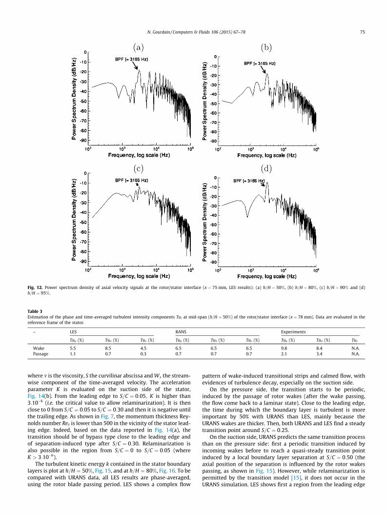
Fig. 12. Power spectrum density of axial velocity signals at the rotor/stator interface (x ¼ 75 mm, LES results): (a) h=H ¼ 50%, (b) h=H ¼ 80%, (c) h=H ¼ 90% and (d)h=H ¼ 95%.

Table 3Estimation of the phase and time-averaged turbulent intensity components Tui at mid-span (h=H ¼ 50%) of the rotor/stator interface (x ¼ 78 mm). Data are evaluated in thereference frame of the stator.

– LES RANS Experiments

Tux (%) Tuh (%) Tur (%) Tux (%) Tuh (%) Tur (%) Tux (%) Tuh (%) Tur

Wake 5.5 8.5 4.5 6.5 6.5 6.5 9.8 8.4 N.A.Passage 1.1 0.7 0.3 0.7 0.7 0.7 2.1 3.4 N.A.

N. Gourdain / Computers & Fluids 106 (2015) 67–78 75

where m is the viscosity, S the curvilinar abscissa and Ws the stream-wise component of the time-averaged velocity. The accelerationparameter K is evaluated on the suction side of the stator,Fig. 14(b). From the leading edge to S=C ¼ 0:05; K is higher than3:10�6 (i.e. the critical value to allow relaminarization). It is thenclose to 0 from S=C ¼ 0:05 to S=C ¼ 0:30 and then it is negative untilthe trailing edge. As shown in Fig. 7, the momentum thickness Rey-nolds number Reh is lower than 500 in the vicinity of the stator lead-ing edge. Indeed, based on the data reported in Fig. 14(a), thetransition should be of bypass type close to the leading edge andof separation-induced type after S=C ¼ 0:30. Relaminarization isalso possible in the region from S=C ¼ 0 to S=C ¼ 0:05 (whereK > 3:10�6).

The turbulent kinetic energy k contained in the stator boundarylayers is plot at h=H ¼ 50%, Fig. 15, and at h=H ¼ 80%, Fig. 16. To becompared with URANS data, all LES results are phase-averaged,using the rotor blade passing period. LES shows a complex flow

pattern of wake-induced transitional strips and calmed flow, withevidences of turbulence decay, especially on the suction side.

On the pressure side, the transition starts to be periodic,induced by the passage of rotor wakes (after the wake passing,the flow come back to a laminar state). Close to the leading edge,the time during which the boundary layer is turbulent is moreimportant by 50% with URANS than LES, mainly because theURANS wakes are thicker. Then, both URANS and LES find a steadytransition point around S=C ¼ 0:25.

On the suction side, URANS predicts the same transition processthan on the pressure side: first a periodic transition induced byincoming wakes before to reach a quasi-steady transition pointinduced by a local boundary layer separation at S=C ¼ 0:50 (theaxial position of the separation is influenced by the rotor wakespassing, as shown in Fig. 15). However, while relaminarization ispermitted by the transition model [15], it does not occur in theURANS simulation. LES shows first a region from the leading edge

Fig. 13. Close view of the instantaneous flow field in the vicinity of the rotor wakes,colored with the viscosity ratio mSGS=m, from LES data at mid-span (h=H ¼ 50%).

Fig. 14. (a) Classification of transition phenomena with respect to the Reynolds number Rthe acceleration parameter K in the present configuration, on the stator suction side, at

Fig. 15. Evolution of the turbulent kinetic energy k inside the stator boundary layer at a wlarger than 0 corresponds to a turbulent boundary layer.

76 N. Gourdain / Computers & Fluids 106 (2015) 67–78

to S=C ¼ �0:40 where the flow is periodically turbulent (likeURANS) and then a second region from S ¼ �0:40 to S=C ¼ �0:50where the flow is laminar (incoming wakes do not have any influ-ence on the state of boundary layers at this location). Data pre-sented in Fig. 14(b) shows a strong acceleration at this locationso it tends to delay transition, as reported in a previous work foranother compressor [10]. Actually, transition is triggered on thesuction side at S=C ¼ 0:50 due to a laminar separation bubble.

Boundary layer transition on the stator vane is driven by twomechanisms: the transition induced by periodic incoming wakesand the quasi-steady transition induced by a laminar separationbubble. This behavior is similar to what has been experimentallyreported by Hobson et al. for a compressor vane at a similar Rey-nolds number [11].

Close to the casing, the same transition mechanisms areobserved, but the transition is also influenced by the tip leakageflow, Fig. 16. LES shows a second peak of turbulent activity at theleading edge, after the rotor wake passing. The tip leakage flowinduces a periodic transition, both on suction and pressure sides.URANS also indicates that the tip leakage flow induces a periodictransition, but only on the pressure side and after S=C ¼ 0:10. This

eh and the acceleration parameter K, as proposed by Mayle [19] and (b) estimation ofh=H ¼ 50%. Relaminarization can occur for K > 3:10�6.

all distance of 100 lm (n=d � 0:03) at h=H ¼ 50%: (a) LES and (b) URANS. Values of k

Fig. 16. Evolution of the turbulent kinetic energy k inside the stator boundary layer at a wall distance of 100 lm (n=d � 0:03) at h=H ¼ 80%: (a) LES and (b) URANS. Values of klarger than 0 corresponds to a turbulent boundary layer. The dotted circle indicates the location of the tip leakage flow.

N. Gourdain / Computers & Fluids 106 (2015) 67–78 77

difference relies on the trajectory of the tip leakage flow, which isdifferent in URANS and LES. The suction side is not affected by thetip leakage flow because the wakes preferentially migrate towardsthe pressure side.

7. Conclusion

This paper describes the analysis of URANS and LES database ina stage of an axial compressor, which operates at operating condi-tions relevant to industrial applications (Mach number M � 0:53and Reynolds number Re ¼ 7� 105). The following points summa-rize this study:

� both LES and URANS show that transition does not occur at theblade and vane leading edges, as it is usually assumed in mostCFD calculations,� comparison with experiments shows that numerical simula-

tions (URANS and LES) underestimate the turbulent intensityat the rotor/stator interface, especially the axial component.As a consequence, the turbulent flow at the entrance of the sta-tor is not correctly represented, which can affect the transitionof stator boundary layer (rotor wake-induced transition),� the spectral analysis of the unsteady flow at the rotor/stator

interface points out that LES predicts frequencies uncorrelatedwith the BPF in the casing region, which are related to the tipleakage flow, while URANS only predicts harmonics of the bladepassing frequency.

Actually a comparison of the transition processes betweennumerical data and experimental measurements is difficult for thistest case. First the inflow conditions are not sufficiently known(turbulent intensity and length scales). It is thus mandatory forfuture researches based on LES and URANS to consider test casewith sufficient measurements to analyze detailed physical mecha-nisms such as those involved in the transition processes (forinstance measurements of the turbulent kinetic energy in theboundary layers). This work shows that LES helps in the under-standing of complex physics, but it is still far to be predictive forturbomachinery flows. Wall-resolved LES data can be used to pro-vide guidelines to develop wall models (including for LES), whichrepresent a good accuracy/cost ratio, especially in the context ofindustrial design.

Acknowledgments

This work has benefited from the help of a lot of people. First,many thanks to H. Miton from Institut Jean Le Rond d’Alembertfor providing experimental data. The author is also grateful toSAFRAN (with a special mention to M. Dumas and G. Leroy for theirconstant help and support). Thanks also to Pr. M. Manna (Univer-sity of Naples) for suggesting some of the post-processings per-formed in this work. The author also thank the CFD team ofCERFACS (with special thanks to J.-F. Boussuge and F. Sicot forreading the manuscript and T. Leonard and A. Gomar for their helpon post-processing). This work has benefited from CERFACS inter-nal and GENCI-TGCC computing facilities (under the projectgen6074). ONERA also provided help and support for the CFD codeelsA. These supports are greatly acknowledged. Actually, the authorwould like to express his sympathy and friendship to the turboma-chinery team of LMFA at Ecole Centrale de Lyon. This paper isdedicated to Pr. Francis Leboeuf.

References

[1] Back SC, Hobson GV, Song SJ, Millsaps KT. Effects of reynolds number andsurface roughness magnitude and location on compressor cascadeperformance. J Turbomach 2012;134(5).

[2] Benyahia A, Houdeville R. Transition prediction in transonic turbineconfigurations using a correlation-based transport equation model. Int J EngSyst Model Simulat 2011;3(1):36–45.

[3] Bhaskaran R, Lele SK. Large eddy simulation of free stream turbulence effectson heat transfer to a high-pressure turbine cascade. J Turbul 2010;11(6).

[4] Bons JP. A review of surface roughness effects in gas turbines. J Turbomach2010;132(2).

[5] Cambier L, Heib S, Plot S. The Onera ElsA CFD software: Input from researchand feedback from industry. Mech Ind 2013;14:159–74.

[6] Faure TM, Michon G-J, Miton H, Vassilieff. Laser doppler anemometrymeasurement in an axial compressor stage. J Propul Power 2001;17(3).

[7] Gourdain N, Prediction of the unsteady turbulent flow in an axial compressorstage. Part 1: Comparison of unsteady RANS and LES data with experiments. JComput Fluids. <http://dx.doi.org/10.1016/j.compfluid.2014.09.052>

[8] Gourdain N, Gicquel L, Montagnac M, Vermorel O, Gazaix M, Staffelbach G,et al. High performance parallel computing of flows in complex geometries –Part 1: Methods. J Comput Sci Discov 2009;2(015003).

[9] Gourdain N, Gicquel LYM, Collado E. Comparison of RANS and LES forprediction of wall heat transfer in a highly loaded turbine guide vane. JPropul Power 2012;28(2):423–33.

[10] Henderson AD, Walker GJ. Observations of transition phenomena on acontrolled diffusion compressor stator with a circular arc leading edge. JTurbomach 2010;132(3).

[11] Hobson GV, Hansen DJ, Schnorenberg DG, Grove DV. Effect of Reynoldsnumber on separation bubbles on compressor blades in cascade. J PropulPower 2001;17(1):154–62.

78 N. Gourdain / Computers & Fluids 106 (2015) 67–78

[12] M. Jahanmiri. Boundary layer transitional flow in gas turbines. TechnicalReport 2011:01, Chalmers University of Technology, 2011.

[13] Jameson A. Time dependent calculations using multigrid, with applications tounsteady flows past airfoils and wings. In: 10th AIAA computational fluiddynamics conference, paper 1596; 1991.

[14] Katz J, Plotkin A. Low-speed aerodynamics. Cambridge aerospace series; 2001.[15] Langtry RB. A correlation-based transition model using local variables for

unstructured parallelized CFD codes. PhD thesis, Stuttgart University; 2006.[16] Langtry RB, Menter FR, Likki SR, Suzen YB. A correlation-based transition

model using local variables – Part 2: Test cases and industrial applications. JTurbomach 2006;128(3).

[17] Manna M, Benocci C, Simons E. Large eddy simulation of turbulent flows viadomain decomposition techniques. Part 1: Theory. Int J Numer Methods Fluids2005;48(4).

[18] Manna M, Vacca A. Effects of the transverse curvature on the statistics of fullydeveloped turbulent flow in an annular pipe. Int J Rotat Mach2002;8(5):353–60.

[19] Mayle RE. The role of laminar-turbulent transition in gas turbine engines. JTurbomach 1991;113(4).

[20] McMullan WA, Page GJ. Towards large eddy simulation of gas turbinecompressors. Prog Aerosp Sci 2012;52:30–47.

[21] Menter FR. Two-equation eddy-viscosity turbulence models for engineeringapplications. AIAA J 1994;32(8).

[22] Menter FR, Langtry RB, Likki SR, Suzen YB. A correlation-based transitionmodel using local variables – Part 1: Model formulation. J Turbomach2006;128(3).

[23] Michelassi V, Wissink JG, Frohlich J, Rodi W. Large-eddy simulation of flowaround low-pressure turbine blade with incoming wakes. AIAA J2003;41(11):2143–56.

[24] Michelassi V, Wissink JG, Rodi W. Direct numerical simulation, large eddysimulation and unsteady Reynolds-averaged Navier–Stokes simulations ofperiodic unsteady flow in a low-pressure turbine cascade: a comparison. ProcInst Mech Eng, Part A: J Power Energy 2003;217(4):403–11.

[25] Michon G-J, Miton H, Ouayahya N. Unsteady three-dimensional off-designvelocity and reynolds stresses in an axial subsonic compressor. J Propul Power2005;21(6).

[26] Nicoud F, Ducros F. Subgrid-scale stress modelling based on the square of thevelocity gradient. Flow, Turbul Combust 1999;62(3):183–200.

[27] Nishikawa H, Rad M, Roe P. A third-order fluctuation splitting scheme thatpreserves potential flow. In: 15th AIAA computational fluid dynamicsconference, paper 2001-2595; 2001.

[28] Piomelli U, Balaras E. Wall-layer models for large-eddy simulations. Annu RevFluid Mech 2002;34.

[29] Raverdy B, Liamis N, Mary I, Sagaut P. High-resolution large-eddy simulationof flow around low-pressure turbine blade. AIAA J 2003;41(3):390–7.

[30] Sicot F, Dufour G, Gourdain N. A time-domain harmonic balance method forrotor/stator interaction. J Turbomach 2012;134(1).

[31] Tucker P, Eastwood S, Klostermeier C, Jefferson-Loveday R, Tyacke J, Liu Y.Hybrid LES approach for practical turbomachinery flows – Part 1: Hierarchyand example simulations. J Turbomach 2012;134(2).

[32] Tucker P, Eastwood S, Klostermeier C, Xia H, Ray P, Tyacke J, et al. Hybrid LESapproach for practical turbomachinery flows – Part 2: Further applications. JTurbomach 2012;134(2).

[33] Yoon S, Jameson A. An LU-SSOR scheme for the Euler and Navier–Stokesequations. In: 25th AIAA aerospace sciences meeting, paper 0600; 1987.