predictive modeling the free hydraulic jumps pressure
TRANSCRIPT

mathematics
Article
Predictive Modeling the Free Hydraulic JumpsPressure through Advanced Statistical Methods
Seyed Nasrollah Mousavi 1 , Renato Steinke Júnior 2 , Eder Daniel Teixeira 2,Daniele Bocchiola 3 , Narjes Nabipour 4 , Amir Mosavi 5,6,7,8 andShahabodin Shamshirband 9,10,*
1 Department of Water Engineering, University of Tabriz, Tabriz 5166616471, Iran; [email protected] Departamento de Obras Hidráulicas, Universidade Federal do Rio Grande do Sul,
Porto Alegre, RS 91.501-970, Brazil; [email protected] (R.S.J.); [email protected] (E.D.T.)3 Department of Civil and Environmental Engineering, Politecnico di Milano, L. da Vinci, 32,
20133 Milano, Italy; [email protected] Institute of Research and Development, Duy Tan University, Da Nang 550000, Vietnam;
[email protected] Institute of Structural Mechanics, Bauhaus Universität Weimar, 99423 Weimar, Germany;
[email protected] Department of Mathematics and Informatics, J. Selye University, 94501 Komarno, Slovakia7 Faculty of Health, Queensland University of Technology, 130 Victoria Park Road,
Brisbane, QLD 4059, Australia8 Kalman Kando Faculty of Electrical Engineering, Obuda University, 1034 Budapest, Hungary9 Department for Management of Science and Technology Development, Ton Duc Thang University,
Ho Chi Minh City, Vietnam10 Faculty of Information Technology, Ton Duc Thang University, Ho Chi Minh City, Vietnam* Correspondence: [email protected]
Received: 25 January 2020; Accepted: 26 February 2020; Published: 2 March 2020�����������������
Abstract: Pressure fluctuations beneath hydraulic jumps potentially endanger the stability of stillingbasins. This paper deals with the mathematical modeling of the results of laboratory-scale experimentsto estimate the extreme pressures. Experiments were carried out on a smooth stilling basin underneathfree hydraulic jumps downstream of an Ogee spillway. From the probability distribution of measuredinstantaneous pressures, pressures with different probabilities could be determined. It was verifiedthat maximum pressure fluctuations, and the negative pressures, are located at the positions nearthe spillway toe. Also, minimum pressure fluctuations are located at the downstream of hydraulicjumps. It was possible to assess the cumulative curves of pressure data related to the characteristicpoints along the basin, and different Froude numbers. To benchmark the results, the dimensionlessforms of statistical parameters include mean pressures (P*m), the standard deviations of pressurefluctuations (σ*X), pressures with different non-exceedance probabilities (P*k%), and the statisticalcoefficient of the probability distribution (Nk%) were assessed. It was found that an existing methodcan be used to interpret the present data, and pressure distribution in similar conditions, by usinga new second-order fractional relationships for σ*X, and Nk%. The values of the Nk% coefficientindicated a single mean value for each probability.
Keywords: mathematical modeling; extreme pressure; hydraulic jump; stilling basin; standarddeviation of pressure fluctuations; statistical coefficient of the probability distribution
1. Introduction
In hydraulic jumps, the high-velocity of an incoming flow abruptly has an impact against a slowerflow [1]. The classical hydraulic jump (CHJ) occurs on the smooth bed of stilling basins. A hydraulic
Mathematics 2020, 8, 323; doi:10.3390/math8030323 www.mdpi.com/journal/mathematics

Mathematics 2020, 8, 323 2 of 16
jump is a phenomenon with non-deterministic characteristics, and for practical purposes, can betreated with the mathematical analysis approaches. Considering that the turbulent pressure nature ishighly random, the analysis is mainly based on mathematical methodologies. Therefore, the stochasticcharacteristics of the problem should be paid attention to [2,3]. This property is a function of theturbulent characteristic of the velocity and pressure field.
Knowledge of pressure fluctuations and extreme pressures allows for a better understanding of theenergy dissipation process along the hydraulic jump. Notable early studies on pressure fluctuations aresuch as those by Bukreyev [4], Locher [5], Schiebe [6], Abdul Khader and Elango [7], Lopardo et al. [8],Lopardo [9], Toso and Bowers [2], Farhoudi and Narayanan [10], Fiorotto and Rinaldo [11], Fiorottoand Rinaldo [12], and Armenio et al. [13].
According to Yan et al. [14], the pressure fluctuations coefficient (C′P) and peak frequencies ofthe spatial hydraulic jumps are higher than the classical jumps. Onitsuka et al. [15] found that rolleroscillations affect the instantaneous flow depth and bed pressure. In addition, the instantaneousbed pressures are associated with free surface fluctuations. Lian et al. [16] stated that the fluctuatingpressure spectrum in the rolling area follows the gravity similarity law. Lopardo and Romagnoli [17]and Lopardo [18] used C′P coefficient values to estimate the turbulence intensities close to the stillingbasin bed for the low incident Froude numbers. Wang et al. [19] predicted the total pressure based uponthe void fraction and velocity data, and the results were in good agreement with the experimental data.Firotto et al. [20] studied the stability of a plunge pool lining under the fully developed jets and proposeda design approach to determine the thickness of the linings. Barjastehmaleki et al. [21] investigatedthe statistical structure of fluctuating pressures within the stilling basins. Barjastehmaleki et al. [22]evaluated an approach for the structural design of stilling basins lining in the sealed and unsealed joints.Lopardo [9] recommended specific flow conditions to measure pressure fluctuations. According tothis, the supercritical Reynolds number (Re1) should be more than 100,000. The minimum acquisitiontime must be 60 seconds. The acquisition frequency can be considered between 50 and 100 Hz.The maximum length of the plastic tube between the pressure tap and transducer is equal to 55 cmwith a minimum inner diameter of 5 mm.
There are some pressure estimation methodologies associated with the hydraulic jumps in theliterature. Gu et al. [23] evaluated the Smoothed Particle Hydrodynamics (SPH) model to estimatethe wave profile, velocity data, and energy dissipation caused by hydraulic jumps. Güven et al. [24]used neural networks to predict the pressure fluctuations on the bed of a sloping stilling basin underB-type hydraulic jump, was investigated in detail by Hager [25]. Teixeira [26] determined the extremepressures with different non-exceedance probabilities (P*k%) from the sample data within a stillingbasin. Teixeira et al. [27] provided the cumulative curves of P*k% for characteristic points along thehydraulic jump. Souza et al. [28] investigated the behavior of the hydraulic jump concerning thelongitudinal distribution of pressures near the bottom of the basin in the low Froude number zone(Fr1 ≤ 4.5). Prá et al. [29] investigated the influence of the vertical curve between the spillway toe andthe stilling basin bed. The results showed that maximum pressure fluctuations were identified at thecenter of the vertical curve and assume values of 1% of the flow kinetic energy at the terminal tangencypoint of the curve. Novakoski et al. [30] investigated extreme pressures with different probabilities(P*k%) on a smooth basin downstream of a stepped spillway. The results showed that the values ofP*0.1% and P*99.9% have lower and higher values than the values observed downstream of the smoothchute, in the region near the spillway toe, respectively.
Pressure distributions along the hydraulic jumps are not described by a normal distribution [31]. Thedistributions of the skewness (S) and kurtosis (K) coefficients of the sample pressure data along the hydraulicjump differ significantly from the value 0, attributed to a normal distribution. This values is observed afterthe endpoint of the hydraulic jump at the dimensionless position X* ≈ 8. According to Marques et al. [31],the distances of pressure points can be dimensionless concerning the conjugate depths, i.e., X* = X/ (Y2
-Y1). Analysis of S and K coefficients displays that there are several types of distributions along hydraulicjumps. Therefore, it is difficult to estimate the pressure data with a certain probability (P*k%). They proposed

Mathematics 2020, 8, 323 3 of 16
dimensionless relationships linking pressure data of P*k% to the mean pressure (P*m), and the standarddeviation of the sample data (σ*X). Such relationships allow us to organize the results of different flowdischarges or Froude numbers and characterize the interest points in hydraulic jumps.
Generally, mean velocity and hydrostatic pressure are considered for designing a stilling basin.However, in the turbulent flow, the characteristics of the fluctuating fields of pressure and velocity maybe more important than the mean values. Accordingly, the design of the stilling basin apron requiresan assessment of the pressures acting upon the bottom of the basin to optimize concrete thickness. It isessential to study the instantaneous pressures beneath the hydraulic jump. There is little informationabout the pressure fluctuations, because it is quite difficult to measure the pressures underneath thehydraulic jump on the bed of stilling basins in the field [15]. Therefore, laboratory-scale experimentscovering pressure fluctuations seem to be reasonable and necessary [32]. Indeed, the United States Bureauof Reclamation (USBR) has provided the general design criteria concerning the stilling basin length,assuming that the hydraulic jump is confined within the stilling basin. However, no indications are givento the different types of hydraulic jump, pressure regime, and forces on the bed of stilling basins [33].
Therefore, the main aim of the present study is to measure and provide useful information aboutthe pressure fluctuations. To do this, the experimental results are compared with those obtainedon the bed of smooth basins in the literature. Many laboratory-scale experiments were designed tosimulate the flow patterns downstream of an Ogee spillway, cascading into a USBR type I stillingbasin, and measuring the pressure fluctuations with a frequency of 20 Hz along the longitudinal axisof the basin. The focus of this study is the mathematical analysis of the extreme pressures distributionat the bottom of a smooth stilling basin for the incident Froude numbers (Fr1) ranging from 7.12to 9.46. New relationships will be proposed for the dimensionless standard deviation (σ*X), andthe statistical coefficient of the probability distribution (Nk%) to estimate the extreme pressures withdifferent non-exceedance probabilities (P*k%).
2. Materials and Methods
2.1. Experimental Setup
Pressure patterns along free hydraulic jumps acting on the bottom of the USBR Type I stillingbasin (smooth bed) downstream of an Ogee spillway, were investigated using a laboratory model(Figure 1). The experiments were conducted in a laboratory Plexiglas-walled flume with 50 cm width,60 cm height, and 10 m length in the hydraulic laboratory at the University of Tabriz, Iran. The flumebed was horizontal. An Ogee spillway with 70 cm height (H), and 61 cm length (L) was equipped witha Type I stilling basin according to the USBR criteria [34].
Mathematics 2020, 8, 323 3 of 16
relationships allow us to organize the results of different flow discharges or Froude numbers and characterize the interest points in hydraulic jumps.
Generally, mean velocity and hydrostatic pressure are considered for designing a stilling basin. However, in the turbulent flow, the characteristics of the fluctuating fields of pressure and velocity may be more important than the mean values. Accordingly, the design of the stilling basin apron requires an assessment of the pressures acting upon the bottom of the basin to optimize concrete thickness. It is essential to study the instantaneous pressures beneath the hydraulic jump. There is little information about the pressure fluctuations, because it is quite difficult to measure the pressures underneath the hydraulic jump on the bed of stilling basins in the field [15]. Therefore, laboratory-scale experiments covering pressure fluctuations seem to be reasonable and necessary [32]. Indeed, the United States Bureau of Reclamation (USBR) has provided the general design criteria concerning the stilling basin length, assuming that the hydraulic jump is confined within the stilling basin. However, no indications are given to the different types of hydraulic jump, pressure regime, and forces on the bed of stilling basins [33].
Therefore, the main aim of the present study is to measure and provide useful information about the pressure fluctuations. To do this, the experimental results are compared with those obtained on the bed of smooth basins in the literature. Many laboratory-scale experiments were designed to simulate the flow patterns downstream of an Ogee spillway, cascading into a USBR type I stilling basin, and measuring the pressure fluctuations with a frequency of 20 Hz along the longitudinal axis of the basin. The focus of this study is the mathematical analysis of the extreme pressures distribution at the bottom of a smooth stilling basin for the incident Froude numbers (Fr1) ranging from 7.12 to 9.46. New relationships will be proposed for the dimensionless standard deviation (σ*X), and the statistical coefficient of the probability distribution (Nk%) to estimate the extreme pressures with different non-exceedance probabilities (P*k%).
2. Materials and Methods
2.1. Experimental Setup
Pressure patterns along free hydraulic jumps acting on the bottom of the USBR Type I stilling basin (smooth bed) downstream of an Ogee spillway, were investigated using a laboratory model (Figure 1). The experiments were conducted in a laboratory Plexiglas-walled flume with 50 cm width, 60 cm height, and 10 m length in the hydraulic laboratory at the University of Tabriz, Iran. The flume bed was horizontal. An Ogee spillway with 70 cm height (H), and 61 cm length (L) was equipped with a Type I stilling basin according to the USBR criteria [34].
Figure 1. Laboratory flume and the experimental setup.

Mathematics 2020, 8, 323 4 of 16
The length of the USBR Type I stilling basin (Lb) was considered 200 cm [35]. The basin width (B)was equal to the flume width (50 cm). The radius of the vertical curve (R) at the spillway toe was 12cm. There was a head tank with 250 cm height to stabilize the flow upstream of the spillway. A hingedweir downstream of the flume was used to control the position of the supercritical depth (Y1) at thespillway toe. The sequent depth (Y2) was measured by an ultrasonic sensor, with an operating inthe range of 10 to 100 cm, and the accuracy of the nominal value the manufacture ±0.1 mm. For theclassical hydraulic jump (CHJ), the most relevant parameter is the incident Froude number (Fr1). TheFroude number characterizes the balance between inertial and gravitational forces. A value of Fr1 > 1indicates the supercritical flow, and vice versa for Fr1 < 1 [36–38].
Fr1 =V1√
g×Y1(1)
V1 =
√2g× (Z−
d0
2) (2)
where V1 is the mean supercritical velocity; d0 is the hydraulic head upstream of the spillway crest; Zis the total water depth upstream of the spillway (Z = H + d0); and g is the gravitational acceleration.The values of Y1 are calculated using the continuity low (Y1 = q/V1), where q is the flow dischargeper unit width. Figure 2 displays some experimental parameters. Figure 3 shows the distribution ofpressure taps along the centerline of the stilling basin. The flow discharge (Q) was measured with anultrasonic flowmeter. Experiments were carried out with different flow discharges in the range of 33 to60.4 L/s. Table 1 presents the range of some experimental parameters along the hydraulic jumps.
Mathematics 2020, 8, 323 4 of 16
Figure 1. Laboratory flume and the experimental setup.
The length of the USBR Type I stilling basin (Lb) was considered 200 cm [35]. The basin width (B) was equal to the flume width (50 cm). The radius of the vertical curve (R) at the spillway toe was 12 cm. There was a head tank with 250 cm height to stabilize the flow upstream of the spillway. A hinged weir downstream of the flume was used to control the position of the supercritical depth (Y1) at the spillway toe. The sequent depth (Y2) was measured by an ultrasonic sensor, with an operating in the range of 10 to 100 cm, and the accuracy of the nominal value the manufacture ±0.1 mm. For the classical hydraulic jump (CHJ), the most relevant parameter is the incident Froude number (Fr1). The Froude number characterizes the balance between inertial and gravitational forces. A value of Fr1 > 1 indicates the supercritical flow, and vice versa for Fr1 < 1 [36–38].
11
1Fr V
g Y=
× (1)
01 2 ( )
2d
V g Z= × −
(2)
where V1 is the mean supercritical velocity; d0 is the hydraulic head upstream of the spillway crest; Z is the total water depth upstream of the spillway (Z = H + d0); and g is the gravitational acceleration. The values of Y1 are calculated using the continuity low (Y1 = q/V1), where q is the flow discharge per unit width. Figure 2 displays some experimental parameters. Figure 3 shows the distribution of pressure taps along the centerline of the stilling basin. The flow discharge (Q) was measured with an ultrasonic flowmeter. Experiments were carried out with different flow discharges in the range of 33 to 60.4 L/s. Table 1 presents the range of some experimental parameters along the hydraulic jumps.
Figure 2. Description of some experimental parameters.
Figure 2. Description of some experimental parameters.
Mathematics 2020, 8, 323 4 of 16
Figure 1. Laboratory flume and the experimental setup.
The length of the USBR Type I stilling basin (Lb) was considered 200 cm [35]. The basin width (B) was equal to the flume width (50 cm). The radius of the vertical curve (R) at the spillway toe was 12 cm. There was a head tank with 250 cm height to stabilize the flow upstream of the spillway. A hinged weir downstream of the flume was used to control the position of the supercritical depth (Y1) at the spillway toe. The sequent depth (Y2) was measured by an ultrasonic sensor, with an operating in the range of 10 to 100 cm, and the accuracy of the nominal value the manufacture ±0.1 mm. For the classical hydraulic jump (CHJ), the most relevant parameter is the incident Froude number (Fr1). The Froude number characterizes the balance between inertial and gravitational forces. A value of Fr1 > 1 indicates the supercritical flow, and vice versa for Fr1 < 1 [36–38].
11
1Fr V
g Y=
× (1)
01 2 ( )
2d
V g Z= × −
(2)
where V1 is the mean supercritical velocity; d0 is the hydraulic head upstream of the spillway crest; Z is the total water depth upstream of the spillway (Z = H + d0); and g is the gravitational acceleration. The values of Y1 are calculated using the continuity low (Y1 = q/V1), where q is the flow discharge per unit width. Figure 2 displays some experimental parameters. Figure 3 shows the distribution of pressure taps along the centerline of the stilling basin. The flow discharge (Q) was measured with an ultrasonic flowmeter. Experiments were carried out with different flow discharges in the range of 33 to 60.4 L/s. Table 1 presents the range of some experimental parameters along the hydraulic jumps.
Figure 2. Description of some experimental parameters.
Figure 3. Distribution of pressure taps along the stilling basin.

Mathematics 2020, 8, 323 5 of 16
Table 1. Experimental parameters along the hydraulic jumps.
Q (L/s) Y1 (cm) Y2 (cm) V1 (m/s) Fr1 (-)
60.4 3.04 27.55 3.89 7.1255.0 2.78 26.49 3.88 7.4452.7 2.66 26.05 3.88 7.5947.5 2.41 24.87 3.87 7.9643.0 2.18 23.70 3.86 8.3433.0 1.68 20.65 3.84 9.46
To measure the instantaneous pressure data, 25 pressure taps were installed at the bottom, alongthe centerline of the stilling basin. Afterward, these data were converted into electrical signals bypressure transducers via a 6-channel digital board. In this study, the transparent plastic tubes wereused with an inner diameter of 3 mm, and the maximum lengths of 200 cm. The six Atek transducers(model BCT–110) had an operating range of -100 to 100 cm of the water column, with the accuracy ofthe nominal value the manufacture ±0.5%. The data acquisition frequency of 20 Hz with a duration of90 seconds was used to collect 1800 sample data for each test and each pressure tap. After processingthe signals using a data acquisition system, the recorded data were displayed using the 6-CH PressureDAQ software.
2.2. Statistical Data Analysis
A series of methodologies to estimate hydraulic pressures under different conditions were used inthe literature. Pressure with a certain non-exceedance probability (Pk%) at the point X can be estimatedusing Equation (3) [31]:
Pk% = Pm + Nk% × σX (3)
where X is the longitudinal distance of each pressure tap from the spillway toe; Pm is the mean pressureat the point X (in cm of water column); Nk% is the dimensionless statistical coefficient of the probabilitydistribution at the point X; σX is the standard deviation of pressure fluctuations at the point X (cm).The dimensionless mean pressure (P*m), and the dimensionless pressure with a certain probability(P*k%) can be expressed as a generic function of X*, and defined as follows [31]:
P∗m =Pm −Y1
Y2 −Y1= f (X∗) = f
(X∗
Y2 −Y1
)(4)
P∗k% =Pk% −Y1
Y2 −Y1= f ′(X∗) (5)
Pressure fluctuations within the hydraulic jumps are related to energy dissipation.The dimensionless standard deviation of pressure fluctuations (σ*X) is defined as follows [31]:
σ∗X =σX
∆E×
Y2
Y1= f ′′ (X∗) (6)
∆E = (Y1 +V2
1
2g) − (Y2 +
V22
2g) (7)
where ∆E is the energy head loss along the hydraulic jump (cm). This parameter depends on theincident Froude number (Fr1), and the distance of the point from the jump toe. Based on Equation(3), Teixeira [26] proposed an estimation method for the extreme pressures with different probabilities(P*k%) along free hydraulic jumps for smooth stilling basins, downstream of spillways. The method isapplied to stable hydraulic jumps (4.5 < Fr1 < 9), and includes the assessment of the dimensionlessstatistical parameters (mean pressures, standard deviation, and statistical probability distribution

Mathematics 2020, 8, 323 6 of 16
coefficient) as a function of X* along stilling basins with the smooth bed. These parameters are definedas follows [26]:
P∗m = −0.015X∗2+ 0.237X∗ + 0.07 0 ≤ X∗ ≤ 8 (8)
σ∗X = −0.159X∗2+ 0.573X∗ + 0.19 0 ≤ X∗ < 2.4 (9)
σ∗X = 0.017X∗2− 0.281X∗ + 1.229 2.4 ≤ X∗ ≤ 8.25 (10)
Nk% = aX∗2+ bX∗ + c 0 ≤ X∗ ≤ 8 (11)
The parameters of a, b, and c vary according to the extreme pressures with different probabilities,and the determination coefficient (R2) [39], are provided in Table 2 [26].
Table 2. Parameters of a, b, and c to estimate Nk% [26].
k% α b c R2
1% +0.0512 −0.4480 −1.6601 0.925% +0.0130 −0.1323 −1.3061 0.7310% +0.0032 −0.0450 −1.0869 0.5990% +0.0048 −0.0325 +1.2695 0.2695% +0.0171 −0.1393 +1.8624 0.8199% +0.0317 −0.3598 +3.3008 0.86
The spatial patterns of the skewness coefficient (S) may be used to highlight the flow detachmentin different zones. The sample skewness coefficient is defined as follows [40,41]:
S =n
(n− 1) × (n− 1)×
∑ni=1 (Pi − Pm)
3
S3X
= f ′′′(X∗) (12)
SX =
√∑ni=1 (Pi − Pm)
2
(n− 1)(13)
where Pi is the instantaneous pressure head at each pressure tap (in cm of water column); SX is thesample standard deviation; and n is the number of data. This value represents the pressure fluctuationsconcerning the mean value of the sample data. A value of S < 0 refers to a longer or fatter tail on theleft side of the density probability function distribution (PDF), and vice versa for S > 0.
The patterns of the kurtosis coefficient (K) in the hydraulic jump confirm the results of the analysisof the pressure fluctuations (σ*X). The value of K is a measure of the spread of data around the meanvalue, characterizing the flatness of the PDF curve. A value of K < 3 indicates the data distributionfunction is more flattened and less concentrated to the mean values compared to a normal distribution,and vice versa for K > 3. The sample kurtosis coefficient is defined as [40,41]:
K =
n× (n + 1)(n− 1) × (n− 2) × (n− 3)
×
∑ni=1 (Pi − Pm)
4
S4X
− 3× (n− 1)2
(n− 2) × (n− 3)= f ′′′′(X∗) (14)
The mathematical analysis of sample pressure data includes the calculation of the values of Pm,σX, Pk%, and Nk%. From the analysis of the probability distribution of sample pressure data, the valuesof Pk% were determined. Then, the dimensionless form of pressure data (P*k%) was taken to comparethe results with different arrangements, obtained from a series of data with different geometries. Theseparameters were analyzed longitudinally, along the stilling basin, and were made dimensionless usingEquations (4)–(6), respectively.

Mathematics 2020, 8, 323 7 of 16
Based on Teixeira [26], the corresponding estimates of the dimensionless statistical parameterswere determined using Equations (8)–(11) and Table 2. Afterward, the parameter of Pm, and σXwere calculated using Equations (4) and (6), respectively. Finally, the estimated values of Pk% wascalculated using Equation (5). To optimize the pressure estimation method proposed by Teixeira [26],new relationships were developed for the parameters of σ*X and Nk%, as a function of X* along thestilling basin. The results of P*k%, obtained from the analysis of the probability distribution of theexperimental data were compared with the corresponding estimated values using the method byTeixeira [26], and the new optimized estimation method proposed in this study.
3. Results and Discussion
3.1. Skewness and Kurtosis Coefficient
Figures 4 and 5 present the distribution of the skewness coefficient (S) and kurtosis coefficient (K),as a function of X* for different Froude numbers. It is found that the pressure distribution along thestilling basin does not follow a normal distribution.
Mathematics. 2020, 10, x 7 of 16
Based on Teixeira [26], the corresponding estimates of the dimensionless statistical parameters
were determined using Equations (8)–(11) and Table 2. Afterward, the parameter of Pm, and σX were
calculated using Equations (4) and (6), respectively. Finally, the estimated values of Pk% was
calculated using Equation (5). To optimize the pressure estimation method proposed by Teixeira [26],
new relationships were developed for the parameters of σ*X and Nk%, as a function of X* along the
stilling basin. The results of P*k%, obtained from the analysis of the probability distribution of the
experimental data were compared with the corresponding estimated values using the method by
Teixeira [26], and the new optimized estimation method proposed in this study.
3. Results and Discussion
3.1. Skewness and Kurtosis Coefficient
Figures 4 and 5 present the distribution of the skewness coefficient (S) and kurtosis coefficient
(K), as a function of X* for different Froude numbers. It is found that the pressure distribution along
the stilling basin does not follow a normal distribution.
Figure 4. Skewness coefficient along the stilling basin.
Figure 5. Kurtosis coefficient along the stilling basin.
From S and K charts, some characteristic points of the hydraulic jump could be defined. These
are the maximum pressure fluctuations point (X*σmax), where the skewness coefficient is high, and Smax
is in the range of 0.5 to 1.5. The position of the flow detachment (X*d), where the skewness coefficient
-1.0
-0.5
0.0
0.5
1.0
1.5
2.0
0 1 2 3 4 5 6 7 8 9
S
X*
Present study
[27]
[31]
-1
0
1
2
3
4
5
6
7
8
9
0 1 2 3 4 5 6 7 8 9
K
X*
Present study
[27]
[31]
Figure 4. Skewness coefficient along the stilling basin.
Mathematics. 2020, 10, x 7 of 16
Based on Teixeira [26], the corresponding estimates of the dimensionless statistical parameters
were determined using Equations (8)–(11) and Table 2. Afterward, the parameter of Pm, and σX were
calculated using Equations (4) and (6), respectively. Finally, the estimated values of Pk% was
calculated using Equation (5). To optimize the pressure estimation method proposed by Teixeira [26],
new relationships were developed for the parameters of σ*X and Nk%, as a function of X* along the
stilling basin. The results of P*k%, obtained from the analysis of the probability distribution of the
experimental data were compared with the corresponding estimated values using the method by
Teixeira [26], and the new optimized estimation method proposed in this study.
3. Results and Discussion
3.1. Skewness and Kurtosis Coefficient
Figures 4 and 5 present the distribution of the skewness coefficient (S) and kurtosis coefficient
(K), as a function of X* for different Froude numbers. It is found that the pressure distribution along
the stilling basin does not follow a normal distribution.
Figure 4. Skewness coefficient along the stilling basin.
Figure 5. Kurtosis coefficient along the stilling basin.
From S and K charts, some characteristic points of the hydraulic jump could be defined. These
are the maximum pressure fluctuations point (X*σmax), where the skewness coefficient is high, and Smax
is in the range of 0.5 to 1.5. The position of the flow detachment (X*d), where the skewness coefficient
-1.0
-0.5
0.0
0.5
1.0
1.5
2.0
0 1 2 3 4 5 6 7 8 9
S
X*
Present study
[27]
[31]
-1
0
1
2
3
4
5
6
7
8
9
0 1 2 3 4 5 6 7 8 9
K
X*
Present study
[27]
[31]
Figure 5. Kurtosis coefficient along the stilling basin.

Mathematics 2020, 8, 323 8 of 16
From S and K charts, some characteristic points of the hydraulic jump could be defined. Theseare the maximum pressure fluctuations point (X*σmax), where the skewness coefficient is high, andSmax is in the range of 0.5 to 1.5. The position of the flow detachment (X*d), where the skewnesscoefficient shifts from a positive value to a negative one (S ≈ 0). The roller endpoint (X*r) indicates theminimum skewness coefficient (Smin). The hydraulic jump endpoint (X*j) is where the streamlinesbecome parallel to the basin bed. At this position, S ≈ 0 and K ≈ 0.
From the previous findings concerning flow statistics, and with analysis of photographs andvideo recordings (not shown for shortness), four characteristic points of the hydraulic jump have beenidentified through the basin, and compare with the findings of Marques et al. [31]. Table 3 presents theapproximate positions of X*σmax, X*d, X*r, and X*j along the stilling basin for different Froude numbers.
Table 3. Approximate positions of the characteristic points.
Fr1 X*σmax X*d X*r X*j
7.12 1.734 3.98 5.81 7.717.44 1.79 4.11 6.01 7.977.59 1.60 3.95 6.09 8.087.96 1.67 3.89 5.45 8.418.34 1.74 3.83 5.69 7.559.46 2.00 4.09 5.40 7.51[31] 1.75 4.00 6.00 8.50
From Table 3, the results for the smooth basin in the present study are qualitatively similarto those reported in the available literature. The values of skewness and kurtosis within the basinare different from those indicated by Marques et al. [31]. In this study, hydrodynamic pressures(measured with transducers) were used to calculate mean pressures, which display oscillatory variations.Marques et al. [31] instead used the hydrostatic pressure (i.e., from water surface profile) to approximatemean pressure. Such an assumption might be the reason for the slight differences, as explained above.
3.2. Cumulative Pressure Curves
From the pressure data with different probabilities (P*k%), the cumulative pressure curves wereprovided for each pressure tap with different Froude numbers. Figure 6 presents the cumulativepressure curves for P*k% related to the characteristic points of X*σmax, X*d, X*r, and X*j, respectively.
Mathematics. 2020, 10, x 8 of 16
shifts from a positive value to a negative one (S ≈ 0). The roller endpoint (X*r) indicates the minimum
skewness coefficient (Smin). The hydraulic jump endpoint (X*j) is where the streamlines become
parallel to the basin bed. At this position, S ≈ 0 and K ≈ 0.
From the previous findings concerning flow statistics, and with analysis of photographs and video
recordings (not shown for shortness), four characteristic points of the hydraulic jump have been identified
through the basin, and compare with the findings of Marques et al. [31]. Table 3 presents the
approximate positions of X*σmax, X*d, X*r, and X*j along the stilling basin for different Froude numbers.
Table 3. Approximate positions of the characteristic points.
Fr1 X*σmax X*d X*r X*j
7.12 1.734 3.98 5.81 7.71
7.44 1.79 4.11 6.01 7.97
7.59 1.60 3.95 6.09 8.08
7.96 1.67 3.89 5.45 8.41
8.34 1.74 3.83 5.69 7.55
9.46 2.00 4.09 5.40 7.51
[31] 1.75 4.00 6.00 8.50
From Table 3, the results for the smooth basin in the present study are qualitatively similar to
those reported in the available literature. The values of skewness and kurtosis within the basin are
different from those indicated by Marques et al. [31]. In this study, hydrodynamic pressures
(measured with transducers) were used to calculate mean pressures, which display oscillatory
variations. Marques et al. [31] instead used the hydrostatic pressure (i.e., from water surface profile)
to approximate mean pressure. Such an assumption might be the reason for the slight differences, as
explained above.
3.2. Cumulative Pressure Curves
From the pressure data with different probabilities (P*k%), the cumulative pressure curves were
provided for each pressure tap with different Froude numbers. Figure 6 presents the cumulative
pressure curves for P*k% related to the characteristic points of X*σmax, X*d, X*r, and X*j, respectively.
Figure 6. Cont.
-0.2
0.0
0.2
0.4
0.6
0.8
1.0
1.2
1.4
0 10 20 30 40 50 60 70 80 90 100
P*
k%
K%
(a)Point 9, Fr1=7.12
Point 9, Fr1=7.44
Point 8, Fr1=7.59
Point 8, Fr1=7.96
Point 8, Fr1=8.34
Point 8, Fr1=9.46
Figure 6. Cont.

Mathematics 2020, 8, 323 9 of 16Mathematics. 2020, 10, x 9 of 16
Figure 6. Cumulative pressure curves for P*k% related to the characteristic points of the hydraulic
jump: (a) X*σmax, (b) X*d, (c) X*r, and (d) X*j.
According to Figure 6, P*k% values increase with increasing probability (k%). Minimum pressure
data (P*min) correspond to the lowest probabilities (P*1%). On the contrary, maximum pressure data
(P*max) correspond to the highest probability (P*99%). Accordingly, the maximum pressure fluctuations,
and the negative pressures, are located at the positions near the spillway toe. Also, the minimum
pressure fluctuations are located at the positions downstream of the hydraulic jump.
3.3. Proposition of New Relationships
Based on the results obtained, it was observed that the method proposed by Teixeira [26] could
be optimized to be used for present data, or in similar conditions by using another relationship for
-0.2
0.0
0.2
0.4
0.6
0.8
1.0
1.2
1.4
0 10 20 30 40 50 60 70 80 90 100
P*k%
K%
(b)
Point 19, Fr1=7.12
Point 19, Fr1=7.44
Point 18, Fr1=7.59
Point 17, Fr1=7.96
Point 16, Fr1=8.34
Point 15, Fr1=9.46
-0.2
0.0
0.2
0.4
0.6
0.8
1.0
1.2
1.4
0 10 20 30 40 50 60 70 80 90 100
P*
k%
K%
(c)
Point 23, Fr1=7.12
Point 23, Fr1=7.44
Point 23, Fr1=7.59
Point 22, Fr1=7.96
Point 22, Fr1=8.34
Point 20, Fr1=9.46
-0.2
0.0
0.2
0.4
0.6
0.8
1.0
1.2
1.4
0 10 20 30 40 50 60 70 80 90 100
P*
k%
K%
(d)
Point 25, Fr1=7.12Point 25, Fr1=7.44Point 25, Fr1=7.59Point 25, Fr1=7.96Point 24, Fr1=8.34Point 23, Fr1=9.46
Figure 6. Cumulative pressure curves for P*k% related to the characteristic points of the hydraulicjump: (a) X*σmax, (b) X*d, (c) X*r, and (d) X*j.
According to Figure 6, P*k% values increase with increasing probability (k%). Minimum pressuredata (P*min) correspond to the lowest probabilities (P*1%). On the contrary, maximum pressure data(P*max) correspond to the highest probability (P*99%). Accordingly, the maximum pressure fluctuations,and the negative pressures, are located at the positions near the spillway toe. Also, the minimumpressure fluctuations are located at the positions downstream of the hydraulic jump.

Mathematics 2020, 8, 323 10 of 16
3.3. Proposition of New Relationships
Based on the results obtained, it was observed that the method proposed by Teixeira [26] could beoptimized to be used for present data, or in similar conditions by using another relationship for thedimensionless standard deviation of pressure fluctuations (σ*X). Thus, a new second-order fractionalrelationship (rational model), as a function of the dimensionless position along the stilling basin,is introduced.
σ∗X =a + bX∗
1 + cX∗ + dX∗20 ≤ X∗ ≤ 7 (15)
where a = 0.3414, b = 0.0299, c = -0.4264, and d = 0.0994. Figure 7 shows the corresponding scatter plotof σ*X, and fitting of Equation (15), with a determination coefficient (R2) equal to 0.776.
Mathematics. 2020, 10, x 10 of 16
the dimensionless standard deviation of pressure fluctuations (σ*X). Thus, a new second-order
fractional relationship (rational model), as a function of the dimensionless position along the stilling
basin, is introduced.
2
**
* *1X
a bX
cX dX
+=
+ + *0 7X (15)
where a = 0.3414, b = 0.0299, c = ‒0.4264, and d = 0.0994. Figure 7 shows the corresponding scatter plot
of σ*X, and fitting of Equation (15), with a determination coefficient (R2) equal to 0.776.
Figure 7. Distribution of σ*X, including the experimental data and Equation (15).
In the present study, the values of Nk% with different non-exceedance probabilities are
determined. Figure 8 shows the longitudinal distribution of the Nk% coefficient.
Figure 8. Distribution of the Nk% coefficient for different probabilities.
From the analysis of Figure 8, the constant values of the coefficient Nk% are developed along the
jump, especially in the case of pressures with probabilities of 5%, 10%, 90%, and 95%. Therefore,
depending on the probability, the values of the coefficient of Nk% indicate a single mean value for
each probability. According to Wiest [42], there is no significant effect of the parameter of Fr1, and the
values of Nk% remain somewhat constant throughout the basin. A new second-order fractional
relationship (rational model) can estimate the Nk% coefficient with a determination coefficient (R2)
equal to 0.98.
% 21k
a bkN
c k d k
+=
+ +
(16)
0.0
0.1
0.2
0.3
0.4
0.5
0.6
0.7
0.8
0.9
1.0
0 1 2 3 4 5 6 7 8 9
σ*X
X*
Fr1=9.46
Fr1=8.34
Fr1=7.96
Fr1=7.59
Fr1=7.44
Fr1=7.12
Equation (15), R2=0.776
-4
-3
-2
-1
0
1
2
3
4
0 1 2 3 4 5
N k
%
X*
N 1% N 5% N 10% N 90% N 95% N 99%
Figure 7. Distribution of σ*X, including the experimental data and Equation (15).
In the present study, the values of Nk% with different non-exceedance probabilities are determined.Figure 8 shows the longitudinal distribution of the Nk% coefficient.
Mathematics. 2020, 10, x 10 of 16
the dimensionless standard deviation of pressure fluctuations (σ*X). Thus, a new second-order
fractional relationship (rational model), as a function of the dimensionless position along the stilling
basin, is introduced.
2
**
* *1X
a bX
cX dX
+=
+ + *0 7X (15)
where a = 0.3414, b = 0.0299, c = ‒0.4264, and d = 0.0994. Figure 7 shows the corresponding scatter plot
of σ*X, and fitting of Equation (15), with a determination coefficient (R2) equal to 0.776.
Figure 7. Distribution of σ*X, including the experimental data and Equation (15).
In the present study, the values of Nk% with different non-exceedance probabilities are
determined. Figure 8 shows the longitudinal distribution of the Nk% coefficient.
Figure 8. Distribution of the Nk% coefficient for different probabilities.
From the analysis of Figure 8, the constant values of the coefficient Nk% are developed along the
jump, especially in the case of pressures with probabilities of 5%, 10%, 90%, and 95%. Therefore,
depending on the probability, the values of the coefficient of Nk% indicate a single mean value for
each probability. According to Wiest [42], there is no significant effect of the parameter of Fr1, and the
values of Nk% remain somewhat constant throughout the basin. A new second-order fractional
relationship (rational model) can estimate the Nk% coefficient with a determination coefficient (R2)
equal to 0.98.
% 21k
a bkN
c k d k
+=
+ +
(16)
0.0
0.1
0.2
0.3
0.4
0.5
0.6
0.7
0.8
0.9
1.0
0 1 2 3 4 5 6 7 8 9
σ*X
X*
Fr1=9.46
Fr1=8.34
Fr1=7.96
Fr1=7.59
Fr1=7.44
Fr1=7.12
Equation (15), R2=0.776
-4
-3
-2
-1
0
1
2
3
4
0 1 2 3 4 5
N k
%
X*
N 1% N 5% N 10% N 90% N 95% N 99%
Figure 8. Distribution of the Nk% coefficient for different probabilities.
From the analysis of Figure 8, the constant values of the coefficient Nk% are developed alongthe jump, especially in the case of pressures with probabilities of 5%, 10%, 90%, and 95%. Therefore,depending on the probability, the values of the coefficient of Nk% indicate a single mean value for eachprobability. According to Wiest [42], there is no significant effect of the parameter of Fr1, and the valuesof Nk% remain somewhat constant throughout the basin. A new second-order fractional relationship(rational model) can estimate the Nk% coefficient with a determination coefficient (R2) equal to 0.98.
Nk% =a + bk
1 + c k + d k2 (16)
Mathematics 2020, 8, 323 11 of 16
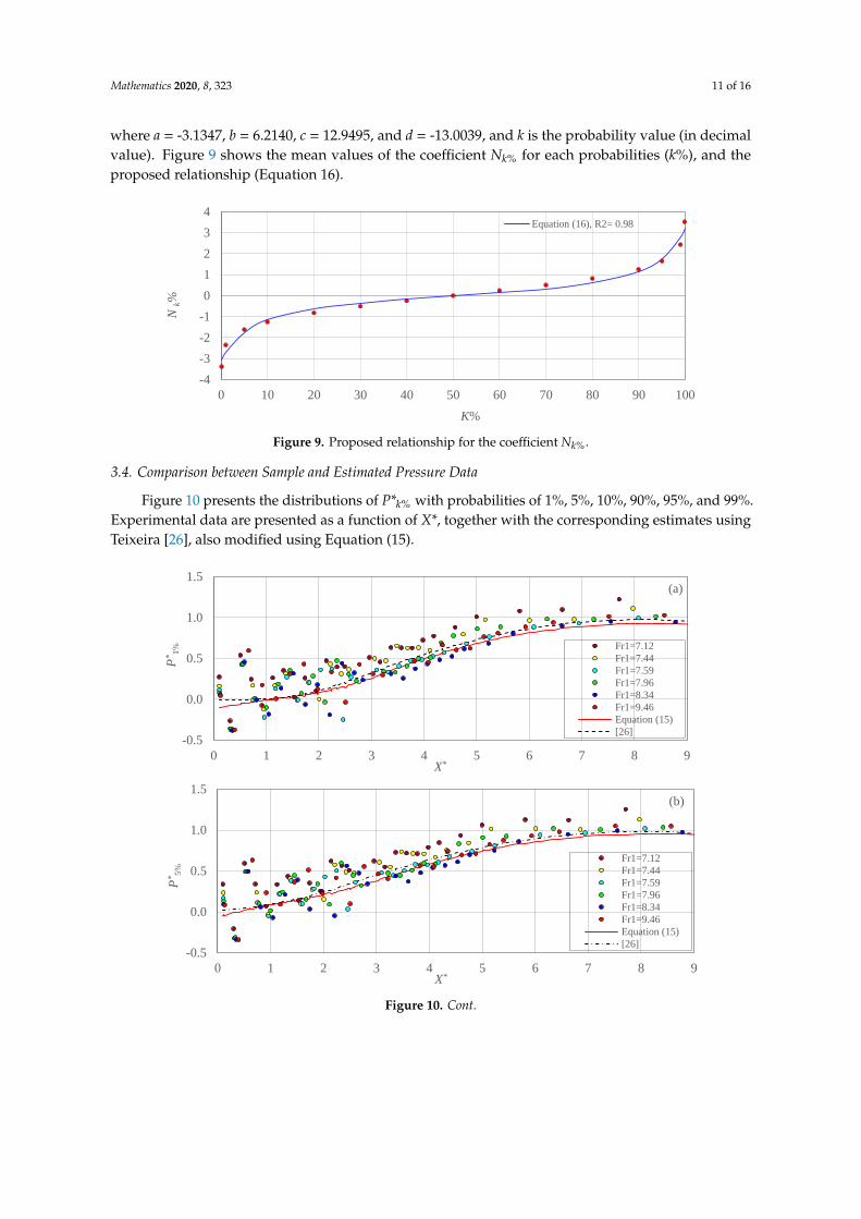
where a = -3.1347, b = 6.2140, c = 12.9495, and d = -13.0039, and k is the probability value (in decimalvalue). Figure 9 shows the mean values of the coefficient Nk% for each probabilities (k%), and theproposed relationship (Equation 16).
Mathematics. 2020, 10, x 11 of 16
where a = ‒3.1347, b = 6.2140, c = 12.9495, and d = ‒13.0039, and k is the probability value (in decimal
value). Figure 9 shows the mean values of the coefficient Nk% for each probabilities (k%), and the
proposed relationship (Equation 16).
Figure 9. Proposed relationship for the coefficient Nk%.
3.4. Comparison between Sample and Estimated Pressure Data
Figure 10 presents the distributions of P*k% with probabilities of 1%, 5%, 10%, 90%, 95%, and 99%.
Experimental data are presented as a function of X*, together with the corresponding estimates using
Teixeira [26], also modified using Equation (15).
Figure 10. Cont.
-4
-3
-2
-1
0
1
2
3
4
0 10 20 30 40 50 60 70 80 90 100
N k
%
K%
Equation (16), R2= 0.98
-0.5
0.0
0.5
1.0
1.5
0 1 2 3 4 5 6 7 8 9
P*1%
X*
(a)
Fr1=7.12
Fr1=7.44
Fr1=7.59
Fr1=7.96
Fr1=8.34
Fr1=9.46
Equation (15)
[26]
-0.5
0.0
0.5
1.0
1.5
0 1 2 3 4 5 6 7 8 9
P*5
%
X*
(b)
Fr1=7.12
Fr1=7.44
Fr1=7.59
Fr1=7.96
Fr1=8.34
Fr1=9.46
Equation (15)
[26]
Figure 9. Proposed relationship for the coefficient Nk%.
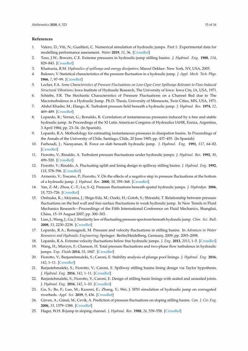
3.4. Comparison between Sample and Estimated Pressure Data
Figure 10 presents the distributions of P*k% with probabilities of 1%, 5%, 10%, 90%, 95%, and 99%.Experimental data are presented as a function of X*, together with the corresponding estimates usingTeixeira [26], also modified using Equation (15).
Mathematics. 2020, 10, x 11 of 16
where a = ‒3.1347, b = 6.2140, c = 12.9495, and d = ‒13.0039, and k is the probability value (in decimal
value). Figure 9 shows the mean values of the coefficient Nk% for each probabilities (k%), and the
proposed relationship (Equation 16).
Figure 9. Proposed relationship for the coefficient Nk%.
3.4. Comparison between Sample and Estimated Pressure Data
Figure 10 presents the distributions of P*k% with probabilities of 1%, 5%, 10%, 90%, 95%, and 99%.
Experimental data are presented as a function of X*, together with the corresponding estimates using
Teixeira [26], also modified using Equation (15).
Figure 10. Cont.
-4
-3
-2
-1
0
1
2
3
4
0 10 20 30 40 50 60 70 80 90 100
N k
%
K%
Equation (16), R2= 0.98
-0.5
0.0
0.5
1.0
1.5
0 1 2 3 4 5 6 7 8 9
P*1%
X*
(a)
Fr1=7.12
Fr1=7.44
Fr1=7.59
Fr1=7.96
Fr1=8.34
Fr1=9.46
Equation (15)
[26]
-0.5
0.0
0.5
1.0
1.5
0 1 2 3 4 5 6 7 8 9
P*5
%
X*
(b)
Fr1=7.12
Fr1=7.44
Fr1=7.59
Fr1=7.96
Fr1=8.34
Fr1=9.46
Equation (15)
[26]
Figure 10. Cont.

Mathematics 2020, 8, 323 12 of 16
Mathematics. 2020, 10, x 12 of 16
Figure 10. Distributions of P*k% with different probabilities: (a) P*1%, (b) P*5%, (c) P*10%, (d) P*90%, (e) P*95%,
and (f) P*99%.
-0.5
0.0
0.5
1.0
1.5
0 1 2 3 4 5 6 7 8 9
P*
10%
X*
(c)
Fr1=7.12
Fr1=7.44
Fr1=7.59
Fr1=7.96
Fr1=8.34
Fr1=9.46
Equation (15)
[26]
-0.5
0.0
0.5
1.0
1.5
0 1 2 3 4 5 6 7 8 9
P*90%
X*
(d)
Fr1=7.12
Fr1=7.44
Fr1=7.59
Fr1=7.96
Fr1=8.34
Fr1=9.46
Equation (15)
[26]
-0.5
0.0
0.5
1.0
1.5
0 1 2 3 4 5 6 7 8 9
P*
95%
X*
(e)
Fr1=7.12
Fr1=7.44
Fr1=7.59
Fr1=7.96
Fr1=8.34
Fr1=9.46
Equation (15)
[26]
-0.5
0.0
0.5
1.0
1.5
0 1 2 3 4 5 6 7 8 9
P*
99
%
X*
(f)
Fr1=7.12
Fr1=7.44
Fr1=7.59
Fr1=7.96
Fr1=8.34
Fr1=9.46
Equation (15)
[26]
Figure 10. Distributions of P*k% with different probabilities: (a) P*1%, (b) P*5%, (c) P*10%, (d) P*90%, (e)P*95%, and (f) P*99%.
Accordingly, close to the spillway toe, pressure data with low and high probability, especiallyfor P*1% and P*99%, have lower and higher values, with the maximum differences than P*m. P*1%
data reach negative values down to -0.2, at the position X* ≈ 2, indicating regions with low pressures.To evaluate the performance of the experimental and the estimated values of σ*X, some statistical

Mathematics 2020, 8, 323 13 of 16
performance criteria including determination coefficient (R2) [39], root mean squared error (RMSE) [39],mean absolute error (MAE) [39], Willmott’s index of agreement (WI) [43] are provided in Table 4. As aresult, the goodness of fit statistics for the estimation of σ*X is confirmed.
Table 4. Results of the statistical performance criteria for σ*X.
Method R2 RMSE MAE WI
Equation (15) 0.776 0.097 0.075 0.931[26] 0.674 0.140 0.115 0.875
For proper performance, RMSE and MAE should be close to zero; and R2 and WI values should beclose to the unit. According to Table 4, this relationship for σ*X provides better estimation performanceas compared against Teixeira [26]. The new relationship is given in Equation (15) presents somewhatbetter results for P*90%, P*95%, and P*99% along the stilling basin.
4. Conclusions
In this study, extreme pressures beneath hydraulic jumps inside the USBR Type I stilling basin(smooth bed) downstream of an Ogee spillway, are investigated for different incident Froude numbersranging from 7.12 to 9.46. In summary, several conclusions are provided as follows:
(1) Sample skewness (S) and kurtosis (K) coefficients indicated that the pressure distribution alongthe hydraulic jumps does not follow a normal distribution. Some characteristic points are themaximum pressure fluctuations point (X*σmax) with Smax; the flow detachment point (X*d) withS ≈ 0; the roller endpoint (X*r) with Smin; and the hydraulic jump endpoint (X*j) with S ≈ 0.
(2) From the pressure data with different non-exceedance probabilities (P*k%), the cumulativepressure curves are presented for P*k% related to the characteristic points of X*σmax, X*d, X*r,and X*j, respectively. For the positions close to the spillway toe, pressures with low and highprobability (P*1% and P*99%), have lower and higher values, with the maximum differences thanP*m. P*1% data, reach negative values down to -0.2, at the position X* ≈ 2, indicating regions withlow pressures.
(3) From the analysis of the probability distribution of the sample data as collected by pressuretransducers, pressures data of P*k% can be determined.
(4) Based on the results obtained, it was observed that the method proposed by Teixeira [26] could beoptimized to be used for present data, or in similar conditions by using another relationship for thedimensionless standard deviation of pressure fluctuations (σ*X), and the statistical coefficient ofthe probability distribution (Nk%). Thus, a new second-order fractional relationship, as a functionof the dimensionless position along the stilling basin (X*), is introduced for σ*X. This relationshipis valid for the dimensionless positions (X*) in the range of 0 to 8.4. To assess the accuracy ofthis relationship, some performance criteria are used. For the new proposed relationship (σ*X) inthis study, the values of R2, RMSE, MAE, and WI were achieved 0.776, 0.097, 0.075, and 0.931,respectively. The constant values of Nk% are developed along the jump. Therefore, depending onthe probability, the values of the Nk% coefficient indicate a single mean value for each probability.A new second-order fractional relationship was proposed to estimate the Nk% coefficient with R2
= 0.98. The new relationships should be validated against sample data taken in similar conditionsto our case study here.
(5) The results contribute to enhancing the knowledge of the flow in a USBR Type I stilling basinthat can be used to improve their design. This work only includes the case of free jumps. Futureadvancements will cover the behavior of submerged jumps with variable submergence degrees,resulting in modified pressure fields concerning those observed here for free jumps. As well,the efficiency of blocks and sills with different sizes may be investigated. A more extensiverange of flow discharge will need to be explored. In the future, the more specific effort may be

Mathematics 2020, 8, 323 14 of 16
devoted to testing other possible distributions, fitting the observed pressure fields and their usein practice design. Also, velocity fields within the hydraulic jump may be investigated to definethe turbulent components of flow fields.
Author Contributions: Conceptualization, N.N., A.M., and S.S.; Data curation, R.S.J. and E.D.T.; Formal analysis,R.S.J. and N.N.; Funding acquisition, S.S.; Investigation, E.D.T. and N.N.; Methodology, S.N.M. and D.B.;Resources, S.N.M.; Software, E.D.T. and D.B.; Supervision, S.N.M. and S.S.; Validation, D.B.; Writing—originaldraft, A.M.; Writing—review & editing, A.M. and S.S. All authors have read and agreed to the published versionof the manuscript
Funding: We acknowledge the financial support of this work by the Hungarian State and the European Unionunder the EFOP-3.6.1-16-2016-00010 project and the 2017-1.3.1-VKE-2017-00025 project.
Acknowledgments: We acknowledge the support of the German Research Foundation (DFG) and theBauhaus-Universität Weimar within the Open-Access Publishing Programme.
Conflicts of Interest: The authors declare no conflict of interest.
Notation
The following symbols are used in this paper:B Basin width (L)Fr1 Incident Froude numberg Gravitational acceleration (LT−2)K Kurtosis coefficientL Spillway length (L)Lb Length of the USBR Type I stilling basin (L)MAE Mean Absolute ErrorNk% Statistical coefficient of probability distribution at point XH Spillway height (L)Pk% Pressure with a certain non-exceedance probability (L)P*k% Dimensionless pressure with a certain non-exceedance probabilityPi Instantaneous pressure of each pressure tap (L)Pm Mean pressure of each pressure tap (L)P*m Dimensionless mean pressure of each pressure tapQ Flow discharge (L3T−1)q Flow discharge per unit width (L2T−1)R1 Hydraulic radius of the incoming flow (L)R2 Determination coefficientRe1 Incident Reynolds numberRMSE Root Mean Squared ErrorS Skewness coefficientSX Sample standard deviationV1 Mean supercritical velocity (LT−1)WI Willmott’s index of agreementX Distance of each pressure tap from the spillway toe (L)X* Dimensionless distance of each pressure tap from the spillway toe, i.e., X/ (Y2 − Y1)X*d Point of the flow detachmentX*j Endpoint of the hydraulic jumpX*r Endpoint of the rollerX*σmax Point of the maximum pressure fluctuationsY1 Supercritical depth (L)Y2 Sequent depth (L)∆E Energy head loss along the hydraulic jump (L)σX Standard deviation of pressure fluctuations at point x (L)
Mathematics 2020, 8, 323 15 of 16
References
1. Valero, D.; Viti, N.; Gualtieri, C. Numerical simulation of hydraulic jumps. Part 1: Experimental data formodelling performance assessment. Water 2019, 11, 36. [CrossRef]
2. Toso, J.W.; Bowers, C.E. Extreme pressures in hydraulic-jump stilling basins. J. Hydraul. Eng. 1988, 114,829–843. [CrossRef]
3. Khatsuria, R.M. Hydraulics of spillways and energy dissipators; Marcel Dekker: New York, NY, USA, 2005.4. Bukreev, V. Statistical characteristics of the pressure fluctuation in a hydraulic jump. J. Appl. Mech. Tech. Phys.
1966, 7, 97–99. [CrossRef]5. Locher, F.A. Some Characteristics of Pressure Fluctuations on Low-Ogee Crest Spillways Relevant to Flow-Induced
Structural Vibrations; Iowa Institute of Hydraulic Research, The University of Iowa: Iowa City, IA, USA, 1971.6. Schiebe, F.R. The Stochastic Characteristics of Pressure Fluctuations on a Channel Bed due to The
Macroturbulence in a Hydraulic Jump. Ph.D. Thesis, University of Minnesota, Twin Cities, MN, USA, 1971.7. Abdul Khader, M.; Elango, K. Turbulent pressure field beneath a hydraulic jump. J. Hydraul. Res. 1974, 12,
469–489. [CrossRef]8. Lopardo, R.; Vernet, G.; Ronaldo, R. Correlation of instantaneous pressures induced by a free and stable
hydraulic jump. In Proceedings of the XI Latin American Congress of Hydraulics IAHR, Ezeiza, Argentina,3 April 1984; pp. 23–34. (In Spanish).
9. Lopardo, R.A. Methodology for estimating instantaneous pressures in dissipation basins. In Proceedings ofthe Annals of the University of Chile, Santiago, Chile, 20 June 1985; pp. 437–455. (In Spanish)
10. Farhoudi, J.; Narayanan, R. Force on slab beneath hydraulic jump. J. Hydraul. Eng. 1991, 117, 64–82.[CrossRef]
11. Fiorotto, V.; Rinaldo, A. Turbulent pressure fluctuations under hydraulic jumps. J. Hydraul. Res. 1992, 30,499–520. [CrossRef]
12. Fiorotto, V.; Rinaldo, A. Fluctuating uplift and lining design in spillway stilling basins. J. Hydraul. Eng. 1992,118, 578–596. [CrossRef]
13. Armenio, V.; Toscano, P.; Fiorotto, V. On the effects of a negative step in pressure fluctuations at the bottomof a hydraulic jump. J. Hydraul. Res. 2000, 38, 359–368. [CrossRef]
14. Yan, Z.-M.; Zhou, C.-T.; Lu, S.-Q. Pressure fluctuations beneath spatial hydraulic jumps. J. Hydrodyn. 2006,18, 723–726. [CrossRef]
15. Onitsuka, K.; Akiyama, J.; Shige-Eda, M.; Ozeki, H.; Gotoh, S.; Shiraishi, T. Relationship between pressurefluctuations on the bed wall and free surface fluctuations in weak hydraulic jump. In New Trends in FluidMechanics Research—Proceedings of the Fifth International Conference on Fluid Mechanics, Shanghai,China, 15–19 August 2007; pp. 300–303.
16. Lian, J.; Wang, J.; Gu, J. Similarity law of fluctuating pressure spectrum beneath hydraulic jump. Chin. Sci. Bull.2008, 53, 2230–2238. [CrossRef]
17. Lopardo, R.A.; Romagnoli, M. Pressure and velocity fluctuations in stilling basins. In Advances in WaterResources and Hydraulic Engineering; Springer: Berlin/Heidelberg, Germany, 2009; pp. 2093–2098.
18. Lopardo, R.A. Extreme velocity fluctuations below free hydraulic jumps. J. Eng. 2013, 2013, 1–5. [CrossRef]19. Wang, H.; Murzyn, F.; Chanson, H. Total pressure fluctuations and two-phase flow turbulence in hydraulic
jumps. Exp. Fluids 2014, 55, 1847. [CrossRef]20. Fiorotto, V.; Barjastehmaleki, S.; Caroni, E. Stability analysis of plunge pool linings. J. Hydraul. Eng. 2016,
142, 1–11. [CrossRef]21. Barjastehmaleki, S.; Fiorotto, V.; Caroni, E. Spillway stilling basins lining design via Taylor hypothesis.
J. Hydraul. Eng. 2016, 142, 1–11. [CrossRef]22. Barjastehmaleki, S.; Fiorotto, V.; Caroni, E. Design of stilling basin linings with sealed and unsealed joints.
J. Hydraul. Eng. 2016, 142, 1–10. [CrossRef]23. Gu, S.; Bo, F.; Luo, M.; Kazemi, E.; Zhang, Y.; Wei, J. SPH simulation of hydraulic jump on corrugated
riverbeds. Appl. Sci. 2019, 9, 436. [CrossRef]24. Güven, A.; Günal, M.; Cevik, A. Prediction of pressure fluctuations on sloping stilling basins. Can. J. Civ. Eng.
2006, 33, 1379–1388. [CrossRef]25. Hager, W.H. B-jump in sloping channel. J. Hydraul. Res. 1988, 26, 539–558. [CrossRef]

Mathematics 2020, 8, 323 16 of 16
26. Teixeira, E.D. Scale effect on estimating extreme pressure values on the bed of the hydraulic dissipationbasins. Ph.D. Thesis, Hydraulic Reseach Institute, Federal University of Rio Grande do Sul, Porto Alegre,Brazil, 2008. (In Portuguese)
27. Teixeira, E.D.; Neto, E.F.T.; Endres, L.A.M.; Marques, M.G. Analysis of pressure fluctuations near the bedin hydraulic jump dissipation basins. In Proceedings of the Brazilian Dam Committee, XXV Large DamsNational Seminar, Salvador, Brazil, 12–15 October 2003; pp. 188–198. (In Portuguese)
28. Souza, P.E.d.A.; Marques, M.G.; Neto, E.F.T.; Teixeira, E.D. Pressure fluctuation in a low-drop and low Froudenumbers of hydraulic jump downstream of a spillway. In Proceedings of the Brazilian Dam Committee, XXX- Large Dams National Seminar, Foz do Iguaçu, Brazil, 11–13 May 2015; pp. 1–14. (In Portuguese)
29. Prá, M.D.; Teixeira, E.D.; Marques, M.G.; Priebe, P.d.S. Evaluation of Pressure Fluctuation in Hydraulic Jumpby Dissociation of Hydraulic Forces. Braz. J. Water Resour. (Rbrh) 2016, 21, 221–231. (In Portuguese)
30. Novakoski, C.K.; Hampe, R.F.; Conterato, E.; Marques, M.G.; Teixeira, E.D. Longitudinal distribution ofextreme pressures in a hydraulic jump downstream of a stepped spillway. Braz. J. Water Resour. (Rbrh) 2017,22, e42. [CrossRef]
31. Marques, M.G.; Drapeau, J.; Verrette, J.-L. Pressure fluctuation coefficient in a hydraulic jump. Braz. J. WaterResour. (Rbrh) 1997, 2, 45–52. (In Portuguese)
32. Farhoudi, J.; Sadat-Helbar, S.; Aziz, N.I. Pressure fluctuation around chute blocks of SAF stilling basins.J. Agric. Sci. Technol. 2010, 12, 203–212.
33. Padulano, R.; Fecarotta, O.; Del Giudice, G.; Carravetta, A. Hydraulic design of a USBR Type II stilling basin.J. Irrig. Drain. Eng. 2017, 143, 04017001. [CrossRef]
34. USBR. Spillways. In Design of small dams, 3rd ed.; US Department of the Interior, Bureau of Reclamation:Washington, DC, USA, 1987; pp. 339–437.
35. Chanson, H.; Carvalho, R. Hydraulic jumps and stilling basins. In Energy Dissipation in Hydraulic Structures;Chanson; CRC Press: Leiden, The Netherlands, 2015; pp. 65–104.
36. Rajaratnam, N. Hydraulic jumps. In Advances in Hydroscience; Elsevier: Edmonton, Canada, 1967; Volume 4,pp. 197–280.
37. Peterka, A.J. Hydraulic Design of Stilling Basins and Energy Dissipators, 8th ed.; U.S. Dept. of the Interior,Bureau of Reclamation: Denver, CO, USA, 1984.
38. Chaudhry, M.H. Open-Channel Flow, 2nd ed.; Springer Science & Business Media: New York, NY, USA, 2008.39. Bennett, N.D.; Croke, B.F.; Guariso, G.; Guillaume, J.H.; Hamilton, S.H.; Jakeman, A.J.; Marsili-Libelli, S.;
Newham, L.T.; Norton, J.P.; Perrin, C. Characterising performance of environmental models. Environ. Model.Softw. 2013, 40, 1–20. [CrossRef]
40. Bono, R.; Arnau, J.; Alarcón, R.; Blanca, M.J. Bias, precision, and accuracy of skewness and kurtosis estimatorsfor frequently used continuous distributions. Symmetry 2020, 12, 19. [CrossRef]
41. Sharma, C.; Ojha, C. Statistical parameters of hydrometeorological variables: standard deviation, SNR,skewness and kurtosis. In Advances in Water Resources Engineering and Management; Springer Singapore:Singapore, 2020; Volume 39, pp. 59–70.
42. Wiest, R.A. Evaluation of the pressure field in hydraulic jump formed downstream of a spillway withdifferent submergence degrees. Master’ Thesis, Hydraulic Reseach Institute, Federal University of RioGrande do Sul, Porto Alegre, Brazil, 2008. (In Portuguese).
43. Willmott, C.J.; Robeson, S.M.; Matsuura, K. A refined index of model performance. Int. J. Climatol. 2012, 32,2088–2094. [CrossRef]
© 2020 by the authors. Licensee MDPI, Basel, Switzerland. This article is an open accessarticle distributed under the terms and conditions of the Creative Commons Attribution(CC BY) license (http://creativecommons.org/licenses/by/4.0/).