preferred and alternative mental models in spatial reasoning · reasoning, and syllogistic...

SPATIAL COGNITION AND COMPUTATION, 5(2&3), 239–269 Copyright © 2005, Lawrence Erlbaum Associates, Inc.

Preferred and Alternative Mental Models in Spatial Reasoning

Reinhold Rauh

University of Freiburg

Markus Knauff University of Freiburg

Max-Planck-Institute for Biological Cybernetics

Christoph Schlieder Bamberg University

Cornelius Hagen Bamberg University

Thomas Kuss

University of Freiburg

Gerhard Strube University of Freiburg

The mental model theory postulates that spatial reasoning relies on the construction, inspection, and the variation of mental models. Experiment 1 shows that in reasoning problems with multiple solutions, reasoners construct only a single model that is preferred over others. Experiment 2 shows that inferences conforming to these preferred mental models (PMM) are easier than inferences that are valid for alternatives. Experiments 3 and 4 support the idea that model variation consists of a model revision process. The process usually starts with the PMM and then constructs alternative models by local transformations. Models which are difficult to reach are more likely to be neglected than models which are only minor revisions of the PMM.

Keywords: Spatial reasoning, mental model, model revision, interval relations, conceptual neighborhood.

Correspondence concerning this article should be addressed to Reinhold Rauh, University of Freiburg, Dept. of Child and Adolescent Psychiatry und Psychotherapy, Hauptstr. 8, 79104 Freiburg, Germany; email: [email protected].

240 RAUH, HAGEN, KNAUFF, KUSS, SCHLIEDER, STRUBE

Processing spatial information is essential to the survival of the species and of the individual. It can concern information from small scale and large scale space. Things get even more complicated if language comes into play and certain organisms have to process spatial information expressed in natural language and draw inferences from this. This will be the type of spatial problems dealt with in this article.

Byrne and Johnson-Laird (1989) devised some ingenious spatial reasoning tasks having marked effects regarding ease of inference. Here is their problem I (Byrne & Johnson-Laird, 1989, p. 567):

I. A is on the right of B C is on the left of B D is in front of C E is in front of B What is the relation between D and E?

Most people correctly infer that D must be left of E. In Experiment 2 of Byrne and Johnson-Laird (1989), 70% of the participants drew this valid conclusion. Now, let’s turn to their problem II:

II. B is on the right of A C is on the left of B D is in front of C E is in front of B What is the relation between D and E?

Problem II differs from problem I only in the first sentence where both entities (A and B) swapped roles. This problem, however, is much harder than problem I, although it endorses the same conclusion, that is, that D must be left of E. Only 46% of the participants (Byrne & Johnson-Laird, 1989, exp. 2) drew this valid conclusion.

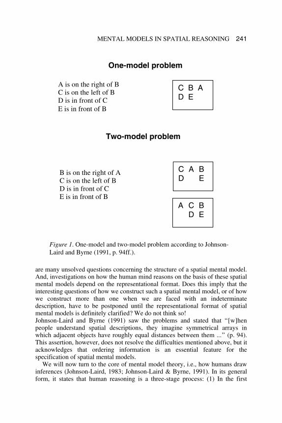
According to Byrne and Johnson-Laird (1989) problem II is more difficult because the more models a problem supports, the harder the inference is. Byrne and Johnson-Laird, therefore, label problem I a one-model problem and problem II a two-model problem (see Figure 1), since description I determines one spatial layout, whereas description II allows for two spatial layouts.

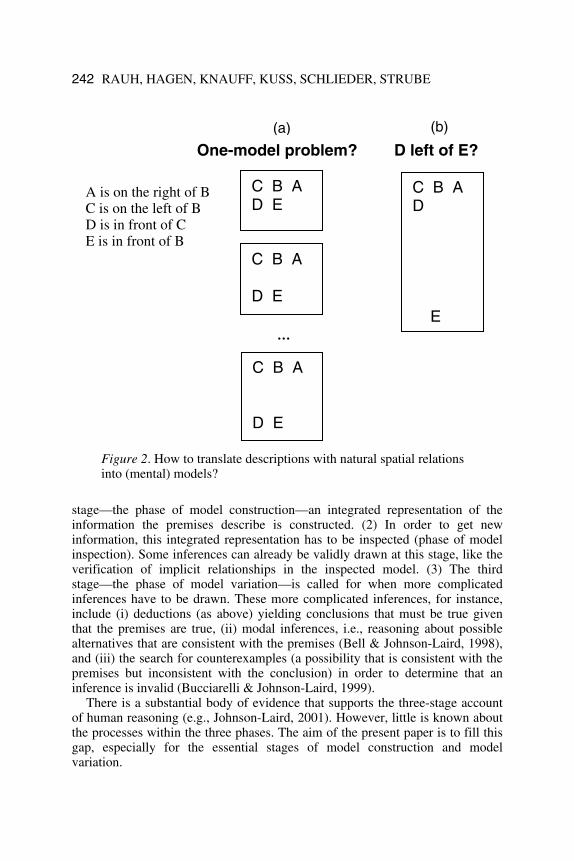
However, what makes problem I a one-model problem? This is difficult to say, because if a model was nothing other than a picture, then problem I describes many pictures, namely an infinite number of metrical variants of diagram 1 (see Figure 2a).

If models were pictures, problem I would be a multiple-model problem, too, and the explanation for the easy-hard difference would be not applicable anymore. Things can get even more complicated. Why, given problem I, not construct the spatial layout like in Figure 2b? And, if so, would you then accept the inference that D is left of E? Probably not. This shows that even the validity of inferences strongly hinges on the meaning of such common relations like left-of, right-of, in-front-of, and so on. In sum, this little example reveals that there

MENTAL MODELS IN SPATIAL REASONING 241

are many unsolved questions concerning the structure of a spatial mental model. And, investigations on how the human mind reasons on the basis of these spatial mental models depend on the representational format. Does this imply that the interesting questions of how we construct such a spatial mental model, or of how we construct more than one when we are faced with an indeterminate description, have to be postponed until the representational format of spatial mental models is definitely clarified? We do not think so! Johnson-Laird and Byrne (1991) saw the problems and stated that “[w]hen people understand spatial descriptions, they imagine symmetrical arrays in which adjacent objects have roughly equal distances between them ...” (p. 94). This assertion, however, does not resolve the difficulties mentioned above, but it acknowledges that ordering information is an essential feature for the specification of spatial mental models.

We will now turn to the core of mental model theory, i.e., how humans draw inferences (Johnson-Laird, 1983; Johnson-Laird & Byrne, 1991). In its general form, it states that human reasoning is a three-stage process: (1) In the first

Figure 1. One-model and two-model problem according to Johnson-Laird and Byrne (1991, p. 94ff.).

A is on the right of B C is on the left of B D is in front of C E is in front of B

B is on the right of A C is on the left of B D is in front of C E is in front of B

One-model problem

Two-model problem

C B A D E

C A B D E

A C B D E


stage—the phase of model construction—an integrated representation of the information the premises describe is constructed. (2) In order to get new information, this integrated representation has to be inspected (phase of model inspection). Some inferences can already be validly drawn at this stage, like the verification of implicit relationships in the inspected model. (3) The third stage—the phase of model variation—is called for when more complicated inferences have to be drawn. These more complicated inferences, for instance, include (i) deductions (as above) yielding conclusions that must be true given that the premises are true, (ii) modal inferences, i.e., reasoning about possible alternatives that are consistent with the premises (Bell & Johnson-Laird, 1998), and (iii) the search for counterexamples (a possibility that is consistent with the premises but inconsistent with the conclusion) in order to determine that an inference is invalid (Bucciarelli & Johnson-Laird, 1999).

There is a substantial body of evidence that supports the three-stage account of human reasoning (e.g., Johnson-Laird, 2001). However, little is known about the processes within the three phases. The aim of the present paper is to fill this gap, especially for the essential stages of model construction and model variation.

Figure 2. How to translate descriptions with natural spatial relations into (mental) models?

A is on the right of B C is on the left of B D is in front of C E is in front of B

One-model problem? D left of E?

C B A D E

C B A D E

C B A D E

…

C B A D E

(b) (a)


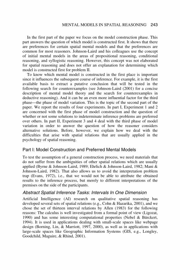
In the first part of the paper we focus on the model construction phase. This part answers the question of which model is constructed first. It shows that there are preferences for certain spatial mental models and that the preferences are common for most reasoners. Johnson-Laird and his colleagues use the concept of initial mental models in the areas of propositional reasoning, conditional reasoning, and syllogistic reasoning. However, this concept was not elaborated for spatial reasoning and does not offer an explanation for determining which model is constructed first for problem II.

To know which mental model is constructed in the first place is important since it influences the subsequent course of inference. For example, it is the first available basis to extract a putative conclusion that will be tested in the following search for counterexamples (see Johnson-Laird (2001) for a concise description of mental model theory and the search for counterexamples in deductive reasoning). And it can be an even more influential factor for the third phase—the phase of model variation. This is the topic of the second part of the paper. We report the results of four experiments. In part I, Experiment 1 and 2 are concerned with the first phase of model construction and the question of whether or not some solutions to indeterminate inference problems are preferred over others. In part II, Experiment 3 and 4 deal with the third phase of model variation in order to answer the question of how the reasoner considers alternative solutions. Before, however, we explain how we deal with the difficulties that arise with spatial relations that are usually applied in the psychology of spatial reasoning.

Part I: Model Construction and Preferred Mental Models

To test the assumption of a general construction process, we need materials that do not suffer from the ambiguities of other spatial relations which are usually applied (Byrne & Johnson-Laird, 1989; Ehrlich & Johnson-Laird, 1982; Mani & Johnson-Laird, 1982). That also allows us to avoid the interpretation problem trap (Evans, 1972), i.e., that we would not be able to attribute the obtained results to the inference process, but merely to different interpretations of the premises on the side of the participants.

Abstract Spatial Inference Tasks: Intervals In One Dimension Artificial Intelligence (AI) research on qualitative spatial reasoning has developed several sets of spatial relations (e.g., Cohn & Hazarika, 2001), and we chose the set of thirteen interval relations by Allen (1983) for the following reasons: The calculus is well investigated from a formal point of view (Ligozat, 1990) and has some interesting computational properties (Nebel & Bürckert, 1994). It is used in applications dealing with small-scale spaces like webpage design (Borning, Lin, & Marriott, 1997, 2000), as well as in applications with large-scale spaces like Geographic Information Systems (GIS, e.g., Longley, Goodchild, Maguire, & Rhind, 2001).


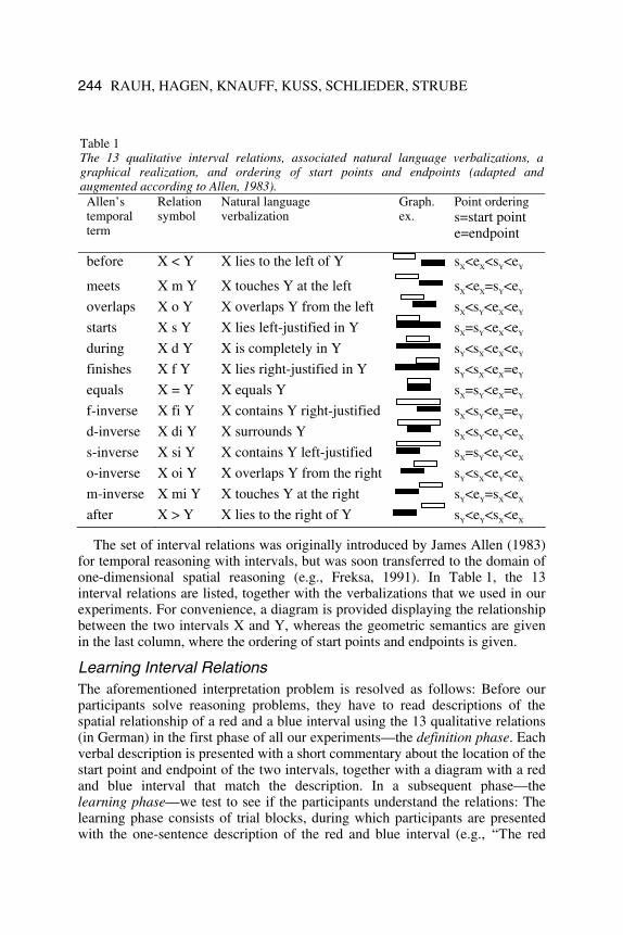
The set of interval relations was originally introduced by James Allen (1983) for temporal reasoning with intervals, but was soon transferred to the domain of one-dimensional spatial reasoning (e.g., Freksa, 1991). In Table 1, the 13 interval relations are listed, together with the verbalizations that we used in our experiments. For convenience, a diagram is provided displaying the relationship between the two intervals X and Y, whereas the geometric semantics are given in the last column, where the ordering of start points and endpoints is given.

Learning Interval Relations The aforementioned interpretation problem is resolved as follows: Before our participants solve reasoning problems, they have to read descriptions of the spatial relationship of a red and a blue interval using the 13 qualitative relations (in German) in the first phase of all our experiments—the definition phase. Each verbal description is presented with a short commentary about the location of the start point and endpoint of the two intervals, together with a diagram with a red and blue interval that match the description. In a subsequent phase—the learning phase—we test to see if the participants understand the relations: The learning phase consists of trial blocks, during which participants are presented with the one-sentence description of the red and blue interval (e.g., “The red

Table 1 The 13 qualitative interval relations, associated natural language verbalizations, a graphical realization, and ordering of start points and endpoints (adapted and augmented according to Allen, 1983). Allen’s temporal term

Relation symbol

Natural language verbalization

Graph. ex.

Point ordering s=start point e=endpoint

before X < Y X lies to the left of Y

sX<eX<sY<eY

meets X m Y X touches Y at the left sX<eX=sY<eY

overlaps X o Y X overlaps Y from the left sX<sY<eX<eY

starts X s Y X lies left-justified in Y sX=sY<eX<eY

during X d Y X is completely in Y sY<sX<eX<eY

finishes X f Y X lies right-justified in Y sY<sX<eX=eY

equals X = Y X equals Y sX=sY<eX=eY

f-inverse X fi Y X contains Y right-justified sX<sY<eX=eY

d-inverse X di Y X surrounds Y sX<sY<eY<eX

s-inverse X si Y X contains Y left-justified sX=sY<eY<eX

o-inverse X oi Y X overlaps Y from the right sY<sX<eY<eX

m-inverse X mi Y X touches Y at the right sY<eY=sX<eX

after X > Y X lies to the right of Y sY<eY<sX<eX


interval surrounds the blue interval”). They then have to indicate the start points and endpoints of the intervals by mouse clicks. After confirmation of the final choices, the participant is told whether the choices are right or wrong. If they are wrong, verbal information about the correct point ordering is given. Trials are presented in blocks of all 13 relations in random order. The learning criterion for one relation is accomplished if the participant gives correct answers in three consecutive blocks of the corresponding relation. The learning phase stops as soon as the participant reaches the learning criterion for all thirteen relations. Only after successful completion of the learning phase does the participant proceed to the actual inference phase of our experiments where we observe and record the types of inferences and response times.

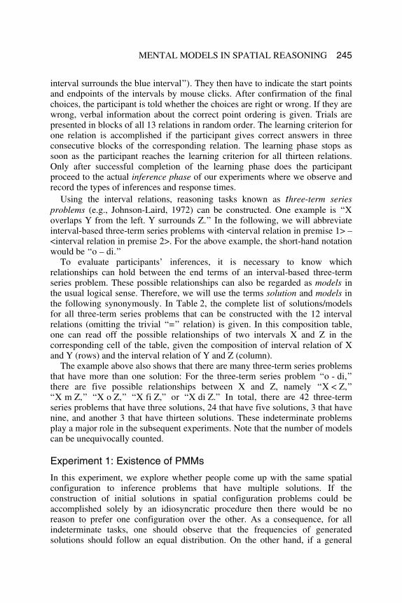
Using the interval relations, reasoning tasks known as three-term series problems (e.g., Johnson-Laird, 1972) can be constructed. One example is “X overlaps Y from the left. Y surrounds Z.” In the following, we will abbreviate interval-based three-term series problems with <interval relation in premise 1> – <interval relation in premise 2>. For the above example, the short-hand notation would be “o – di.”

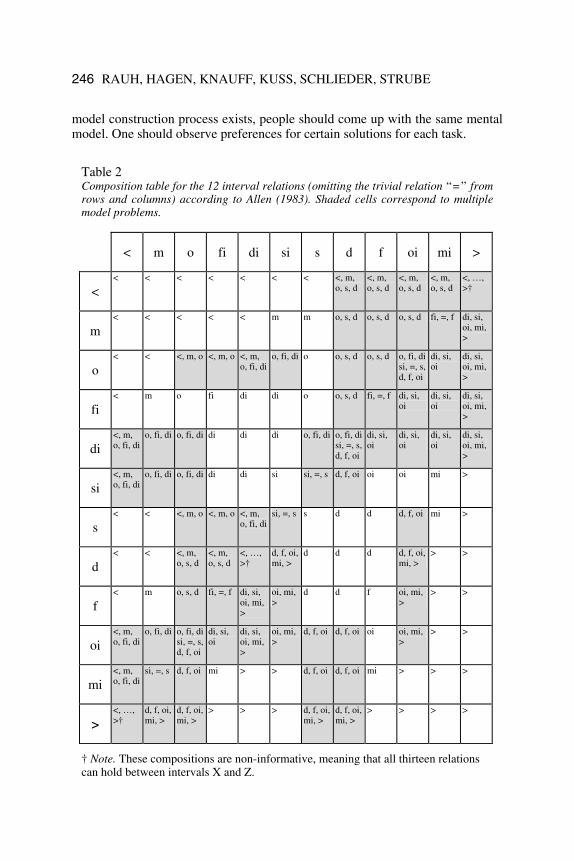
To evaluate participants’ inferences, it is necessary to know which relationships can hold between the end terms of an interval-based three-term series problem. These possible relationships can also be regarded as models in the usual logical sense. Therefore, we will use the terms solution and models in the following synonymously. In Table 2, the complete list of solutions/models for all three-term series problems that can be constructed with the 12 interval relations (omitting the trivial “=” relation) is given. In this composition table, one can read off the possible relationships of two intervals X and Z in the corresponding cell of the table, given the composition of interval relation of X and Y (rows) and the interval relation of Y and Z (column).

The example above also shows that there are many three-term series problems that have more than one solution: For the three-term series problem “o - di,” there are five possible relationships between X and Z, namely “X < Z,” “X m Z,” “X o Z,” “X fi Z,” or “X di Z.” In total, there are 42 three-term series problems that have three solutions, 24 that have five solutions, 3 that have nine, and another 3 that have thirteen solutions. These indeterminate problems play a major role in the subsequent experiments. Note that the number of models can be unequivocally counted.

Experiment 1: Existence of PMMs

In this experiment, we explore whether people come up with the same spatial configuration to inference problems that have multiple solutions. If the construction of initial solutions in spatial configuration problems could be accomplished solely by an idiosyncratic procedure then there would be no reason to prefer one configuration over the other. As a consequence, for all indeterminate tasks, one should observe that the frequencies of generated solutions should follow an equal distribution. On the other hand, if a general


model construction process exists, people should come up with the same mental model. One should observe preferences for certain solutions for each task.

Table 2 Composition table for the 12 interval relations (omitting the trivial relation “=” from rows and columns) according to Allen (1983). Shaded cells correspond to multiple model problems.

< m o fi di si s d f oi mi >

< < < < < < < < <, m,

o, s, d <, m, o, s, d

<, m, o, s, d

<, m, o, s, d

<, …, >†

m < < < < < m m o, s, d o, s, d o, s, d fi, =, f di, si,

oi, mi, >

o < < <, m, o <, m, o <, m,

o, fi, dio, fi, di o o, s, d o, s, d o, fi, di

si, =, s, d, f, oi

di, si, oi

di, si, oi, mi, >

fi < m o fi di di o

o, s, d fi, =, f di, si,

oi di, si, oi

di, si, oi, mi, >

di <, m, o, fi, di

o, fi, di o, fi, di di di di o, fi, di o, fi, di si, =, s, d, f, oi

di, si, oi

di, si, oi

di, si, oi

di, si, oi, mi, >

si <, m, o, fi, di

o, fi, di o, fi, di di di si si, =, s d, f, oi oi oi mi >

s < < <, m, o <, m, o <, m,

o, fi, disi, =, s s d d d, f, oi mi >

d < < <, m,

o, s, d <, m, o, s, d

<, …, >†

d, f, oi, mi, >

d d d d, f, oi, mi, >

> >

f < m o, s, d fi, =, f di, si,

oi, mi, >

oi, mi, >

d d f oi, mi, >

> >

oi <, m, o, fi, di

o, fi, di o, fi, di si, =, s, d, f, oi

di, si, oi

di, si, oi, mi, >

oi, mi, >

d, f, oi d, f, oi oi oi, mi, >

> >

mi <, m, o, fi, di

si, =, s d, f, oi mi > > d, f, oi d, f, oi mi > > >

> <, …, >†

d, f, oi, mi, >

d, f, oi, mi, >

> > > d, f, oi, mi, >

d, f, oi, mi, >

> > > >

† Note. These compositions are non-informative, meaning that all thirteen relations can hold between intervals X and Z.


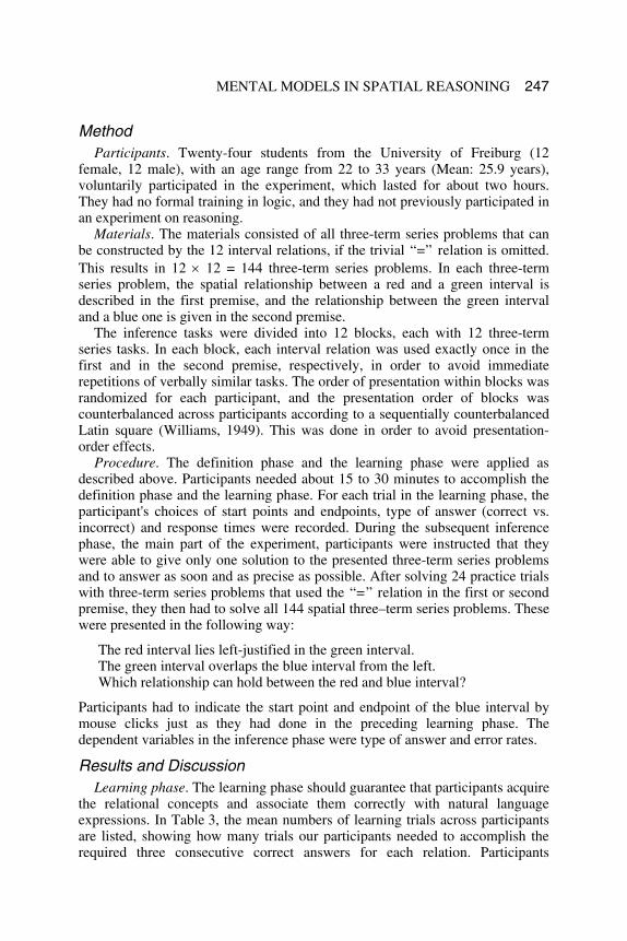
Method Participants. Twenty-four students from the University of Freiburg (12

female, 12 male), with an age range from 22 to 33 years (Mean: 25.9 years), voluntarily participated in the experiment, which lasted for about two hours. They had no formal training in logic, and they had not previously participated in an experiment on reasoning.

Materials. The materials consisted of all three-term series problems that can be constructed by the 12 interval relations, if the trivial “=” relation is omitted. This results in 12 × 12 = 144 three-term series problems. In each three-term series problem, the spatial relationship between a red and a green interval is described in the first premise, and the relationship between the green interval and a blue one is given in the second premise.

The inference tasks were divided into 12 blocks, each with 12 three-term series tasks. In each block, each interval relation was used exactly once in the first and in the second premise, respectively, in order to avoid immediate repetitions of verbally similar tasks. The order of presentation within blocks was randomized for each participant, and the presentation order of blocks was counterbalanced across participants according to a sequentially counterbalanced Latin square (Williams, 1949). This was done in order to avoid presentation-order effects.

Procedure. The definition phase and the learning phase were applied as described above. Participants needed about 15 to 30 minutes to accomplish the definition phase and the learning phase. For each trial in the learning phase, the participant's choices of start points and endpoints, type of answer (correct vs. incorrect) and response times were recorded. During the subsequent inference phase, the main part of the experiment, participants were instructed that they were able to give only one solution to the presented three-term series problems and to answer as soon and as precise as possible. After solving 24 practice trials with three-term series problems that used the “=” relation in the first or second premise, they then had to solve all 144 spatial three–term series problems. These were presented in the following way:

The red interval lies left-justified in the green interval. The green interval overlaps the blue interval from the left. Which relationship can hold between the red and blue interval?

Participants had to indicate the start point and endpoint of the blue interval by mouse clicks just as they had done in the preceding learning phase. The dependent variables in the inference phase were type of answer and error rates.

Results and Discussion Learning phase. The learning phase should guarantee that participants acquire

the relational concepts and associate them correctly with natural language expressions. In Table 3, the mean numbers of learning trials across participants are listed, showing how many trials our participants needed to accomplish the required three consecutive correct answers for each relation. Participants


understood the relation “=” at once (M = 3.00) whereas they needed the most learning trials for the relation “mi” (M = 3.83). As expected, the pattern was nearly the same for the related measure of the percentage of correct responses (see Table 3). From these results, we can conclude (i) that our learning phase was successful, (ii) that the interval relations can be acquired and associated with natural language expressions, and (iii) adoption is accomplished within a reasonable time scale. However, the most important point is that the following results of the inference phase are (almost) not affected by interpretational fluctuations of the inference tasks.

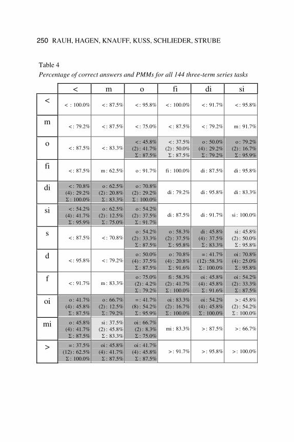
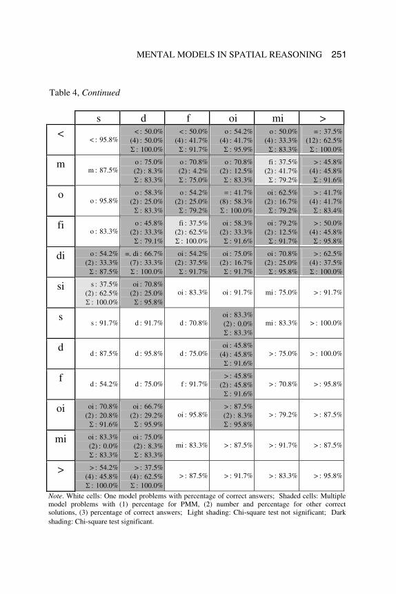
Existence of PMMs. To test the global hypothesis that solutions for all three-term series problems with multiple models (i.e., 72 out of 144 problems; see shaded cells in Table 2) are not equally distributed, a chi-square test was conducted that yielded a significant result, χ2(240) = 1583.82, p < .001. This corroborates the assumption that there are general preferred solutions in spatial reasoning with the interval relations. Testing the 72 multiple model problems separately, we obtained statistically significant chi-square values in 65 out of 72 tests (see Table 4 for details). The most impressive example is the problem “s – oi” (The red interval lies left-justified in the green interval. The green interval overlaps the blue interval from the right.), where 83.3% of our participants chose the relation “oi” (The red interval overlaps the blue interval from the right.), whereas the other two correct relations “d” and “f” (see Table 4) were never produced.

The findings replicate the results of Knauff, Rauh, and Schlieder (1995) who used a different drawing procedure. Again we found evidence for a general construction process for spatial configurations that operates the same way for the majority of people. The preferences in both studies revealed a concordance rate of 59 out of 72 (79.1%) problems with multiple solutions.

How can PMMs be explained? The conceptual representation of the relations might be one reason for our findings. The spatial relations could be represented as prototypes that convey metrical information in order to construct typical situations. For instance, the metrical prototype of the “overlaps from the right” relation could incorporate a distance parameter that specifies the proportional length of two intervals in order to produce the prototypical “overlaps-from-the-right” situation. Thus, several distance parameters could be specified and attached to each relation. That is the approach that Berendt (1996) accomplished for the interval relations, taking into account (i) that the set of parameters should generate only images that are actual models of the premises and (ii) reproduces

Table 3 Mean number of learning trials and percentage correct for all 13 interval relations

< m o fi di si = s d f oi mi > Mean 3.42 3.63 3.46 3.21 3.13 3.01 3.00 3.33 3.08 3.08 3.58 3.83 3.29 Perc. 95.1 88.5 88.0 95.0 98.6 97.3 100 98.6 96.1 96.0 87.2 89.1 94.9


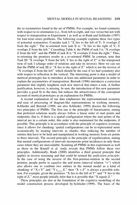
the (a-)symmetries found in the set of PMMs. For example, we found symmetry with respect to re-orientation (i.e., from left-to-right, and vice versa) but not with respect to transposition in Experiment 1 as well as in Rauh and Schlieder (1997) for four-term series problems. The following example explains these two types of potential symmetries: Consider task I “X lies to the left of Y; Y overlaps Z from the right.” The re-oriented twin task II is: “X lies to the right of Y; Y overlaps Z from the left.” Consulting Table 4, the PMM of task I is “X overlaps Z from the left” and the PMM of task II is “X overlaps Z from the right.” Thus, re-orienting the premises results in a re-oriented PMM. In contrast, note that Task III “X overlaps Y from the left; Y lies to the right of Z” is the transposed twin of task I (change order of relations and take its inverse). Here we can see that the PMM of task III is “X lies to the right of Z” which is not the inverse of “X overlaps Z from the left” which should be the case if we had symmetry also with respect to reflection in the vertical. The interesting point is that a model of metrical prototypes has to introduce at least one additional parameter in order to explain the asymmetries of transposition. Berendt (1996) introduces a correction parameter that slightly lengthens each new interval that enters a task. A further justification, however, is missing. In sum, the introduction of this new parameter provides a good fit to the data, but reduces the attractiveness of the conceptual account of metrical prototypes as an explanation for PMMs.

A second explanation of our data emphasizes the representational economy and ease of processing of diagram-like representations in working memory. Schlieder and Berendt (1998; see also Schlieder, 1999) discuss the following two principles of PMMs: The first one is the principle of linearization, stating that preferred solutions nearly always follow a linear order of start points and endpoints; that is, if there is a spatial configuration where the start points of the interval are in a certain order, this order is also maintained for the endpoints, if possible. This principle is in accordance with the principle of cognitive economy since it allows for chunking: spatial configurations can be re-represented more economically by treating intervals as chunks, thus reducing the number of entities that have to be held and manipulated in working memory from six points to three intervals. The second principle is the principle of regularization, stating that mental configurations of intervals incorporate point incidences in only those cases where they are unavoidable. Scanning all PMMs in this experiment as well as those in the Knauff et al. study reveals that PMMs follow these two principles. Additionally, Rauh (2000) identifies a third general principle that applies in inverse reasoning and that could be termed the unification principle: In the case of using the inverse of the first-premise-relation in the second premise, people prefer to equalize the end terms (interval relation “=”) which also allows one to combine two entities in the mental model as a kind of chunking: if “X r Y” and “Y rinverse Z,” then “X = Z” is always a possible solu-tion. For example, given the premises “X lies to the left of Y” and “Y lies to the right of Z,” most people initially infer that it is possible that “X equals Z.”

These principles are also at the foundation of the cognitive modelling of the model construction process developed by Schlieder (1999). The basis of the


Table 4

Percentage of correct answers and PMMs for all 144 three-term series tasks

< m o fi di si <

< : 100.0%

< : 87.5% < : 95.8% < : 100.0% < : 91.7%

< : 95.8%

m < : 79.2%

< : 87.5% < : 75.0% < : 87.5% < : 79.2%

m : 91.7%

o < : 87.5% < : 83.3%

< : 45.8%(2) : 41.7%

Σ : 87.5%

< : 37.5%(2) : 50.0%

Σ : 87.5%

o : 50.0%(4) : 29.2%

Σ : 79.2%

o : 79.2% (2) : 16.7%

Σ : 95.9%

fi < : 87.5%

m : 62.5% o : 91.7% fi : 100.0% di : 87.5%

di : 95.8%

di < : 70.8% (4) : 29.2% Σ : 100.0%

o : 62.5%(2) : 20.8%

Σ : 83.3%

o : 70.8%(2) : 29.2%Σ : 100.0%

di : 79.2% di : 95.8%

di : 83.3%

si < : 54.2% (4) : 41.7%

Σ : 95.9%

o : 62.5%(2) : 12.5%

Σ : 75.0%

o : 54.2%(2) : 37.5%

Σ : 91.7%di : 87.5% di : 91.7%

si : 100.0%

s < : 87.5% < : 70.8%

o : 54.2%(2) : 33.3%

Σ : 87.5%

o : 58.3%(2) : 37.5%

Σ : 95.8%

di : 45.8%(4) : 37.5%

Σ : 83.3%

si : 45.8% (2) : 50.0%

Σ : 95.8%

d < : 95.8% < : 79.2%

o : 50.0%(4) : 37.5%

Σ : 87.5%

o : 70.8%(4) : 20.8%

Σ : 91.6%

= : 41.7%(12) :58.3%Σ : 100.0%

oi : 70.8% (4) : 25.0%

Σ : 95.8%

f < : 91.7% m : 83.3%

o : 75.0%(2) : 4.2%Σ : 79.2%

fi : 58.3%(2) : 41.7%Σ : 100.0%

oi : 45.8%(4) : 45.8%

Σ : 91.6%

oi : 54.2% (2) : 33.3%

Σ : 87.5%

oi o : 41.7% (4) : 45.8%

Σ : 87.5%

o : 66.7%(2) : 12.5%

Σ : 79.2%

= : 41.7%(8) : 54.2%

Σ : 95.9%

oi : 83.3%(2) : 16.7%Σ : 100.0%

oi : 54.2%(4) : 45.8%Σ : 100.0%

> : 45.8% (2) : 54.2% Σ : 100.0%

mi o : 45.8% (4) : 41.7%

Σ : 87.5%

si : 37.5%(2) : 45.8%

Σ : 83.3%

oi : 66.7%(2) : 8.3%Σ : 75.0%

mi : 83.3% > : 87.5%

> : 66.7%

> = : 37.5% (12) : 62.5%

Σ : 100.0%

oi : 45.8%(4) : 41.7%

Σ : 87.5%

oi : 41.7%(4) : 45.8%

Σ : 87.5%> : 91.7% > : 95.8%

> : 100.0%


Table 4, Continued

s d f oi mi > <

< : 95.8% < : 50.0%

(4) : 50.0%Σ : 100.0%

< : 50.0%(4) : 41.7%

Σ : 91.7%

o : 54.2%(4) : 41.7%

Σ : 95.9%

o : 50.0%(4) : 33.3%

Σ : 83.3%

= : 37.5% (12) : 62.5%

Σ : 100.0%

m m : 87.5%

o : 75.0%(2) : 8.3%Σ : 83.3%

o : 70.8%(2) : 4.2%Σ : 75.0%

o : 70.8%(2) : 12.5%

Σ : 83.3%

fi : 37.5%(2) : 41.7%

Σ : 79.2%

> : 45.8% (4) : 45.8%

Σ : 91.6%

o o : 95.8%

o : 58.3%(2) : 25.0% Σ : 83.3%

o : 54.2%(2) : 25.0%

Σ : 79.2%

= : 41.7%(8) : 58.3%Σ : 100.0%

oi : 62.5%(2) : 16.7%

Σ : 79.2%

> : 41.7% (4) : 41.7%

Σ : 83.4%

fi o : 83.3%

o : 45.8%(2) : 33.3%

Σ : 79.1%

fi : 37.5%(2) : 62.5%Σ : 100.0%

oi : 58.3%(2) : 33.3%

Σ : 91.6%

oi : 79.2%(2) : 12.5%

Σ : 91.7%

> : 50.0% (4) : 45.8%

Σ : 95.8%

di o : 54.2% (2) : 33.3%

Σ : 87.5%

=. di : 66.7%(7) : 33.3%Σ : 100.0%

oi : 54.2%(2) : 37.5%

Σ : 91.7%

oi : 75.0%(2) : 16.7%

Σ : 91.7%

oi : 70.8%(2) : 25.0%

Σ : 95.8%

> : 62.5% (4) : 37.5% Σ : 100.0%

si s : 37.5% (2) : 62.5% Σ : 100.0%

oi : 70.8%(2) : 25.0%

Σ : 95.8%oi : 83.3% oi : 91.7% mi : 75.0%

> : 91.7%

s s : 91.7% d : 91.7% d : 70.8%

oi : 83.3%(2) : 0.0%Σ : 83.3%

mi : 83.3%

> : 100.0%

d d : 87.5% d : 95.8% d : 75.0%

oi : 45.8%(4) : 45.8%

Σ : 91.6%> : 75.0%

> : 100.0%

f d : 54.2% d : 75.0% f : 91.7%

> : 45.8%(2) : 45.8%

Σ : 91.6%> : 70.8%

> : 95.8%

oi oi : 70.8% (2) : 20.8%

Σ : 91.6%

oi : 66.7%(2) : 29.2%

Σ : 95.9%oi : 95.8%

> : 87.5%(2) : 8.3%Σ : 95.8%

> : 79.2%

> : 87.5%

mi oi : 83.3% (2) : 0.0% Σ : 83.3%

oi : 75.0%(2) : 8.3%Σ : 83.3%

mi : 83.3% > : 87.5% > : 91.7%

> : 87.5%

> > : 54.2% (4) : 45.8% Σ : 100.0%

> : 37.5%(4) : 62.5%Σ : 100.0%

> : 87.5% > : 91.7% > : 83.3%

> : 95.8%

Note. White cells: One model problems with percentage of correct answers; Shaded cells: Multiple model problems with (1) percentage for PMM, (2) number and percentage for other correct solutions, (3) percentage of correct answers; Light shading: Chi-square test not significant; Dark shading: Chi-square test significant.


cognitive modelling is an ordinal representation of start points and endpoints. A spatial focus operates on this ordinal representation and inserts the points of new intervals according to special insertion schemes that are specified for each interval relation. A cognitive modelling of the model construction process is available as a JAVA applet (Schlieder et al., 2002) together with further information on the model construction process.

Experiment 2: PMM-Verification Bias

The existence of PMMs suggests that the verification of a relationship which holds in the PMM is easier, because the relevant information is available as soon as the PMM is constructed. In contrast, the verification of relationships being solely valid in alternative models of the premises should be harder, because the construction of the PMM demands working memory resources, causing a delay in the construction of alternative models, and may even cause a failure to build them. Experiment 2 tested this assumption using a verification paradigm.

Method Participants. Twenty-six students from the University of Freiburg, 13 female

and 13 male with an age range from 21 to 36 years, were paid for participating in the experiment, which lasted for about two hours. Again, they had no formal training in logic, and they had not previously participated in an experiment on reasoning.

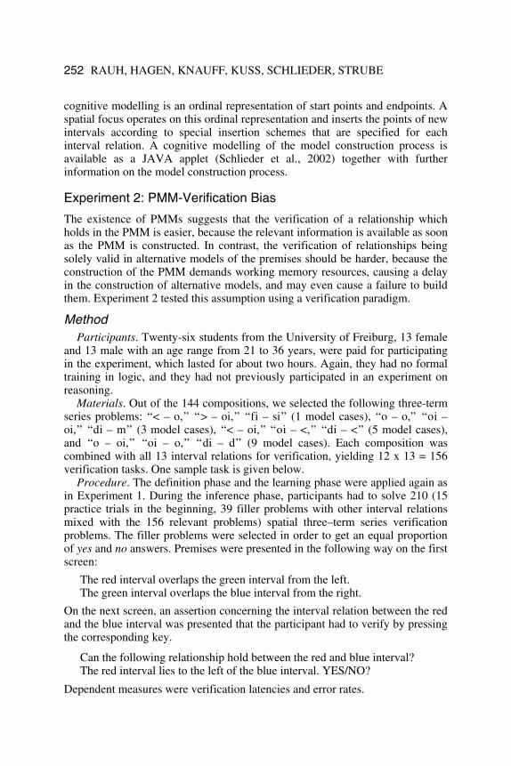
Materials. Out of the 144 compositions, we selected the following three-term series problems: “< – o,” “> – oi,” “fi – si” (1 model cases), “o – o,” “oi – oi,” “di – m” (3 model cases), “< – oi,” “oi – <,” “di – <” (5 model cases), and “o – oi,” “oi – o,” “di – d” (9 model cases). Each composition was combined with all 13 interval relations for verification, yielding 12 x 13 = 156 verification tasks. One sample task is given below.

Procedure. The definition phase and the learning phase were applied again as in Experiment 1. During the inference phase, participants had to solve 210 (15 practice trials in the beginning, 39 filler problems with other interval relations mixed with the 156 relevant problems) spatial three–term series verification problems. The filler problems were selected in order to get an equal proportion of yes and no answers. Premises were presented in the following way on the first screen:

The red interval overlaps the green interval from the left. The green interval overlaps the blue interval from the right.

On the next screen, an assertion concerning the interval relation between the red and the blue interval was presented that the participant had to verify by pressing the corresponding key.

Can the following relationship hold between the red and blue interval? The red interval lies to the left of the blue interval. YES/NO?

Dependent measures were verification latencies and error rates.


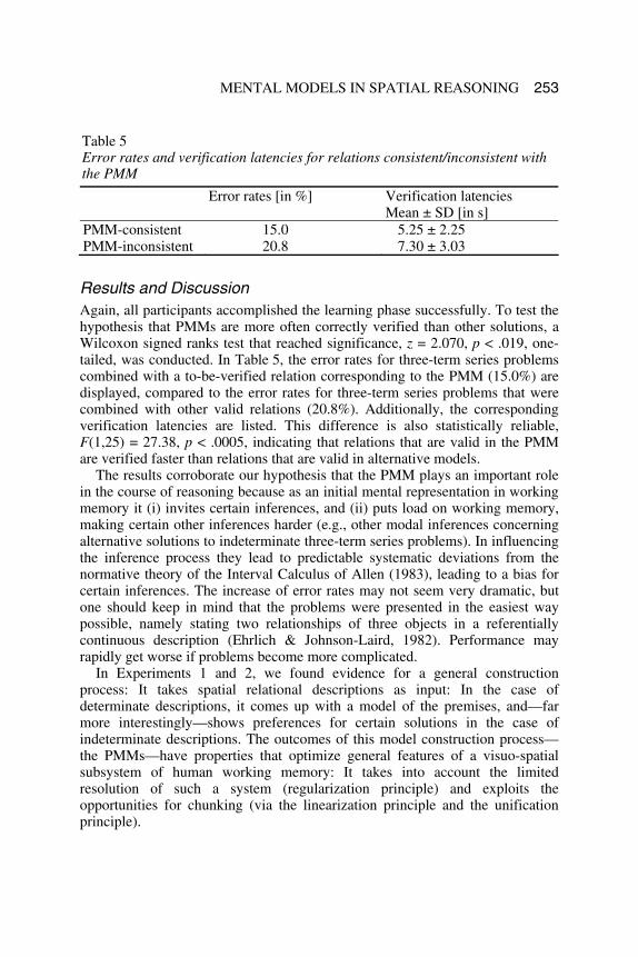
Results and Discussion Again, all participants accomplished the learning phase successfully. To test the hypothesis that PMMs are more often correctly verified than other solutions, a Wilcoxon signed ranks test that reached significance, z = 2.070, p < .019, one-tailed, was conducted. In Table 5, the error rates for three-term series problems combined with a to-be-verified relation corresponding to the PMM (15.0%) are displayed, compared to the error rates for three-term series problems that were combined with other valid relations (20.8%). Additionally, the corresponding verification latencies are listed. This difference is also statistically reliable, F(1,25) = 27.38, p < .0005, indicating that relations that are valid in the PMM are verified faster than relations that are valid in alternative models.

The results corroborate our hypothesis that the PMM plays an important role in the course of reasoning because as an initial mental representation in working memory it (i) invites certain inferences, and (ii) puts load on working memory, making certain other inferences harder (e.g., other modal inferences concerning alternative solutions to indeterminate three-term series problems). In influencing the inference process they lead to predictable systematic deviations from the normative theory of the Interval Calculus of Allen (1983), leading to a bias for certain inferences. The increase of error rates may not seem very dramatic, but one should keep in mind that the problems were presented in the easiest way possible, namely stating two relationships of three objects in a referentially continuous description (Ehrlich & Johnson-Laird, 1982). Performance may rapidly get worse if problems become more complicated.

In Experiments 1 and 2, we found evidence for a general construction process: It takes spatial relational descriptions as input: In the case of determinate descriptions, it comes up with a model of the premises, and—far more interestingly—shows preferences for certain solutions in the case of indeterminate descriptions. The outcomes of this model construction process—the PMMs—have properties that optimize general features of a visuo-spatial subsystem of human working memory: It takes into account the limited resolution of such a system (regularization principle) and exploits the opportunities for chunking (via the linearization principle and the unification principle).

Table 5 Error rates and verification latencies for relations consistent/inconsistent with the PMM

Error rates [in %] Verification latencies Mean ± SD [in s]

PMM-consistent 15.0 5.25 ± 2.25 PMM-inconsistent 20.8 7.30 ± 3.03


Part II: Model Revision and Alternative Mental Models

The phase of model variation, or the validation phase as Johnson-Laird and Byrne (1991) prefer to say in the case of deductive inference, is at the heart of the inference process: “Only in the third stage is any essential deductive work carried out: the first two stages are merely normal processes of comprehension and description” (Johnson-Laird & Byrne, 1991, p. 36). Much recent work has concentrated on this stage, especially in propositional and syllogistic reasoning. Again, for spatial reasoning no such studies exist.

For all areas of reasoning, two general classes of processes/strategies of the phase of model variation are conceivable: Either there is an iteration of model construction and model inspection, in which each mental model is constructed from scratch (model iteration) accompanied with an mechanism to avoid endless loops of constructing the same model over and over again, or there is a model revision process that takes the previous mental model to revise it in order to come to the next one. Since from the psychology of thinking it is known that human cognition heavily relies on previous information, e.g., use of old solutions in case-based reasoning (Kolodner, 1993), set effects in problem-solving (Anderson, 2000), or anchoring effects in judgment and decision making (Tversky & Kahneman, 1974), model revision seems the more plausible candidate. Again, the questions arise whether there is a general model revision process, and how the revision is accomplished. From AI research of Qualitative Spatial Reasoning (QSR) and Diagrammatic Reasoning (DR, see Schlieder, 1998), we import the promising notion of local transformation as a method for mental model revision. We will describe the concept of local transformation in more detail in the following section.

Generating the Sequence of Solutions via Local Transformations Since different models of a three-term series problem can be unequivocally distinguished by the relation between X and Z, we can treat models and relations equivalently. Thus, a transformation is a transition from one relation r1 to another relation r2. We will abbreviate this as r1 → r2 in the following.

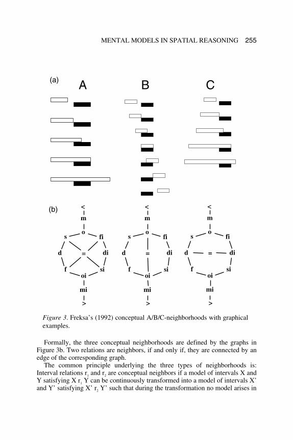
Freksa (1992) introduced the notion of a conceptual neighborhood between interval relations that has three variants that are the consequence of three distinct types of local transformations. The A-neighborhood is based on a transformation that can be described as the movement of one single boundary point of one interval, whereas the B-neighborhood relies on the movement of a complete interval of fixed length. The transformation defining the C-neighborhood consists of keeping the center of the changing interval fixed, and varying its length. The types of transformations defining the A(B, C)-neighborhoods will be called A(B, C)-transformations (see Figure 3a for some pictorial examples of local transformations).


Formally, the three conceptual neighborhoods are defined by the graphs in

Figure 3b. Two relations are neighbors, if and only if, they are connected by an edge of the corresponding graph.

The common principle underlying the three types of neighborhoods is: Interval relations r1 and r2 are conceptual neighbors if a model of intervals X and Y satisfying X r1 Y can be continuously transformed into a model of intervals X’ and Y’ satisfying X’ r2 Y’ such that during the transformation no model arises in

Figure 3. Freksa’s (1992) conceptual A/B/C-neighborhoods with graphical examples.

m

os

d

foi

mi

>

fi

di

si

=

<

m

o s

d

f oi

mi

>

fi

di

si

=

<

m

os

d

foi

mi

>

fi

di

si

=

<

A B C (a)

(b)


which a relation different from r1 and r2 holds (see Schlieder & Hagen, 2000). Their peculiarities arise from different transformation processes (see Figure 3).

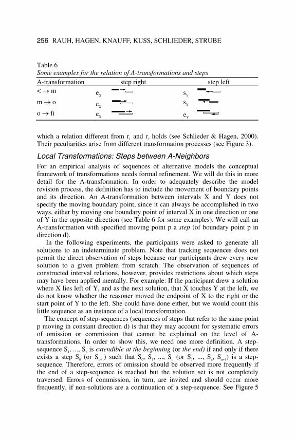
Local Transformations: Steps between A-Neighbors For an empirical analysis of sequences of alternative models the conceptual framework of transformations needs formal refinement. We will do this in more detail for the A-transformation. In order to adequately describe the model revision process, the definition has to include the movement of boundary points and its direction. An A-transformation between intervals X and Y does not specify the moving boundary point, since it can always be accomplished in two ways, either by moving one boundary point of interval X in one direction or one of Y in the opposite direction (see Table 6 for some examples). We will call an A-transformation with specified moving point p a step (of boundary point p in direction d).

In the following experiments, the participants were asked to generate all solutions to an indeterminate problem. Note that tracking sequences does not permit the direct observation of steps because our participants drew every new solution to a given problem from scratch. The observation of sequences of constructed interval relations, however, provides restrictions about which steps may have been applied mentally. For example: If the participant drew a solution where X lies left of Y, and as the next solution, that X touches Y at the left, we do not know whether the reasoner moved the endpoint of X to the right or the start point of Y to the left. She could have done either, but we would count this little sequence as an instance of a local transformation.

The concept of step-sequences (sequences of steps that refer to the same point p moving in constant direction d) is that they may account for systematic errors of omission or commission that cannot be explained on the level of A-transformations. In order to show this, we need one more definition. A step-sequence S1, ..., Sn is extendible at the beginning (or the end) if and only if there exists a step S0 (or Sn+1) such that S0, S1, ..., Sn (or S1, ..., Sn, Sn+1) is a step-sequence. Therefore, errors of omission should be observed more frequently if the end of a step-sequence is reached but the solution set is not completely traversed. Errors of commission, in turn, are invited and should occur more frequently, if non-solutions are a continuation of a step-sequence. See Figure 5

Table 6 Some examples for the relation of A-transformations and steps A-transformation step right step left < → m eX sY m → o eX sY

o → fi eX eY


for an example where an error of commission is invited, and Figure 6 for a 5-model problem that is prone to an error of omission.

Experiment 3: Constructing Alternative Models

Our general assumption is that moving along a step-sequence, i.e., keeping the moving point and its direction constant, is the easiest way to generate alternative solutions. More complicated processes would result from changing the moving point, changing direction, or even performing a non-local transformation. In the following, we present hypotheses specifying the implications of the above considerations in more detail. They are illustrated in Table 6 and Figure 4.

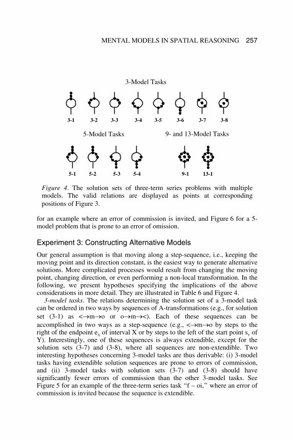
3-model tasks. The relations determining the solution set of a 3-model task can be ordered in two ways by sequences of A-transformations (e.g., for solution set (3-1) as <→m→o or o→m→<). Each of these sequences can be accomplished in two ways as a step-sequence (e.g., <→m→o by steps to the right of the endpoint eX of interval X or by steps to the left of the start point sY of Y). Interestingly, one of these sequences is always extendible, except for the solution sets (3-7) and (3-8), where all sequences are non-extendible. Two interesting hypotheses concerning 3-model tasks are thus derivable: (i) 3-model tasks having extendible solution sequences are prone to errors of commission, and (ii) 3-model tasks with solution sets (3-7) and (3-8) should have significantly fewer errors of commission than the other 3-model tasks. See Figure 5 for an example of the three-term series task “f – oi,” where an error of commission is invited because the sequence is extendible.

3-Model Tasks

5-Model Tasks 9- and 13-Model Tasks

3-1 3-2 3-3 3-4 3-5 3-6 3-7 3-8

5-1 5-2 5-3 5-4 9-1 13-1

Figure 4. The solution sets of three-term series problems with multiple models. The valid relations are displayed as points at corresponding positions of Figure 3.


5-model tasks. The solution set of a 5-model task can be ordered in two ways by sequences of A-transformations. Each of these sequences can also be accomplished in two ways, as a step-sequence that is non-extendible, or as a sequence S1, S2, S3, S4, where S1, S2 and S3, S4 are non-extendible step-sequences, having the same direction but referring to different boundary points of the same interval. Accordingly, we can formulate the hypothesis that errors of omission will most frequently occur between step 2 and step 3 (see Figure 6 for an example where the boundary point has to be changed in order to reach the remaining two solutions).

9-model tasks and 13-model tasks. The solution set of a 9-model task or of a 13-model task can be ordered in multiple ways by sequences of A-transformations. Each of them falls into several step-sequences, including necessary changes of direction between them. Therefore, we expect a decreased number of correct and complete solution sequences for these tasks.

Method Participants. A different set of twenty-four students from the University of

Freiburg (12 female, 12 male) without formal training in logic were paid for their participation in the experiment that lasted for about 2 to 2.5 hours.

Materials. The materials consisted of the 72 indeterminate three-term series problems that can be constructed by the 12 interval relations if the trivial “=” relation is omitted. In each three-term series problem, the spatial relationship between a red and a green interval is described in the first premise, and the

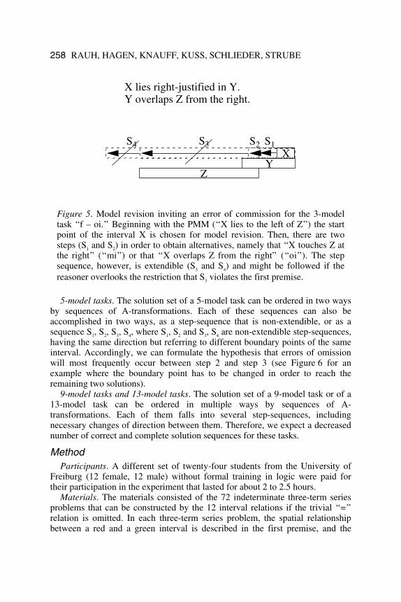
Figure 5. Model revision inviting an error of commission for the 3-model task “f – oi.” Beginning with the PMM (“X lies to the left of Z”) the start point of the interval X is chosen for model revision. Then, there are two steps (S1 and S2) in order to obtain alternatives, namely that “X touches Z at the right” (“mi”) or that “X overlaps Z from the right” (“oi”). The step sequence, however, is extendible (S3 and S4) and might be followed if the reasoner overlooks the restriction that S3 violates the first premise.

X lies right-justified in Y.Y overlaps Z from the right.

S2S3S 4 S1X

YZ


relationship between the green interval and a blue one is given in the second premise.

Procedure. The definition phase and the learning phase were administered like in the previous two experiments. For the learning phase, a minor modification was introduced in order to be consistent with the procedure of the inference phase: The participants had to indicate the spatial relationship of both intervals by mouse clicks.

During the inference phase, participants were given 3 practice trials (without feedback on correctness of solutions), and then received the 72 indeterminate three-term series problems. After self-paced reading of the premises, the premises vanished, and the participants were asked to generate all possible relationships between the red and the blue interval. By clicking the mouse they specified the spatial relationships analogous to the interval-specifying procedure in the learning phase. After finishing the configuration, participants could either continue specifying other solutions, or stop working on the present task and go to the next three-term series problem.

We recorded premise processing times, drawing times, and, most importantly, the sequence of solutions by pixel coordinates and by interval relations.

Results and Discussion All participants passed the learning phase successfully. First, we tested the hypothesis that solution sequences followed the principles of the conceptual

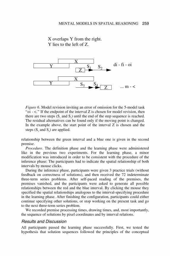
Figure 6. Model revision inviting an error of omission for the 5-model task “oi - <.” If the endpoint of the interval Z is chosen for model revision, then there are two steps (S1 and S2) until the end of the step sequence is reached. The residual alternatives can be found only if the moving point is changed. In the example above, the start point of the interval Z is chosen and the steps (S3 and S4) are applied.

di - fi - oi

... m - <

S1

S3

S2

S4

X overlaps Y from the right.Y lies to the left of Z.

X

X

Y

Y Z

Z


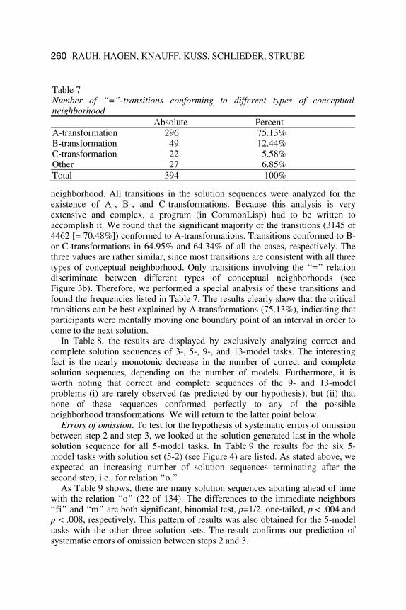
neighborhood. All transitions in the solution sequences were analyzed for the existence of A-, B-, and C-transformations. Because this analysis is very extensive and complex, a program (in CommonLisp) had to be written to accomplish it. We found that the significant majority of the transitions (3145 of 4462 [= 70.48%]) conformed to A-transformations. Transitions conformed to B- or C-transformations in 64.95% and 64.34% of all the cases, respectively. The three values are rather similar, since most transitions are consistent with all three types of conceptual neighborhood. Only transitions involving the “=” relation discriminate between different types of conceptual neighborhoods (see Figure 3b). Therefore, we performed a special analysis of these transitions and found the frequencies listed in Table 7. The results clearly show that the critical transitions can be best explained by A-transformations (75.13%), indicating that participants were mentally moving one boundary point of an interval in order to come to the next solution.

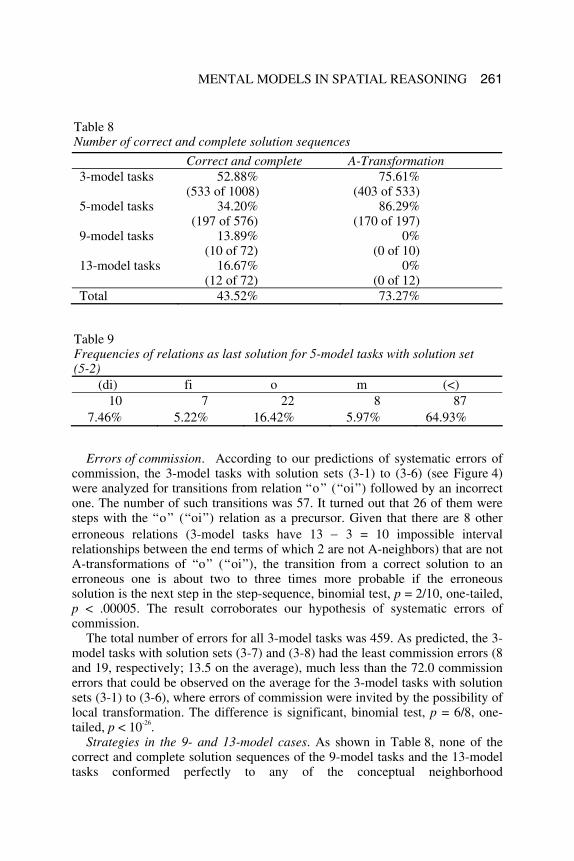
In Table 8, the results are displayed by exclusively analyzing correct and complete solution sequences of 3-, 5-, 9-, and 13-model tasks. The interesting fact is the nearly monotonic decrease in the number of correct and complete solution sequences, depending on the number of models. Furthermore, it is worth noting that correct and complete sequences of the 9- and 13-model problems (i) are rarely observed (as predicted by our hypothesis), but (ii) that none of these sequences conformed perfectly to any of the possible neighborhood transformations. We will return to the latter point below.

Errors of omission. To test for the hypothesis of systematic errors of omission between step 2 and step 3, we looked at the solution generated last in the whole solution sequence for all 5-model tasks. In Table 9 the results for the six 5-model tasks with solution set (5-2) (see Figure 4) are listed. As stated above, we expected an increasing number of solution sequences terminating after the second step, i.e., for relation “o.”

As Table 9 shows, there are many solution sequences aborting ahead of time with the relation “o” (22 of 134). The differences to the immediate neighbors “fi” and “m” are both significant, binomial test, p=1/2, one-tailed, p < .004 and p < .008, respectively. This pattern of results was also obtained for the 5-model tasks with the other three solution sets. The result confirms our prediction of systematic errors of omission between steps 2 and 3.

Table 7 Number of “=”-transitions conforming to different types of conceptual neighborhood Absolute Percent A-transformation 296 75.13% B-transformation 49 12.44% C-transformation 22 5.58% Other 27 6.85% Total 394 100%


Errors of commission. According to our predictions of systematic errors of

commission, the 3-model tasks with solution sets (3-1) to (3-6) (see Figure 4) were analyzed for transitions from relation “o” (“oi”) followed by an incorrect one. The number of such transitions was 57. It turned out that 26 of them were steps with the “o” (“oi”) relation as a precursor. Given that there are 8 other erroneous relations (3-model tasks have 13 − 3 = 10 impossible interval relationships between the end terms of which 2 are not A-neighbors) that are not A-transformations of “o” (“oi”), the transition from a correct solution to an erroneous one is about two to three times more probable if the erroneous solution is the next step in the step-sequence, binomial test, p = 2/10, one-tailed, p < .00005. The result corroborates our hypothesis of systematic errors of commission.

The total number of errors for all 3-model tasks was 459. As predicted, the 3-model tasks with solution sets (3-7) and (3-8) had the least commission errors (8 and 19, respectively; 13.5 on the average), much less than the 72.0 commission errors that could be observed on the average for the 3-model tasks with solution sets (3-1) to (3-6), where errors of commission were invited by the possibility of local transformation. The difference is significant, binomial test, p = 6/8, one-tailed, p < 10-26.

Strategies in the 9- and 13-model cases. As shown in Table 8, none of the correct and complete solution sequences of the 9-model tasks and the 13-model tasks conformed perfectly to any of the conceptual neighborhood

Table 8 Number of correct and complete solution sequences

Correct and complete A-Transformation 3-model tasks 52.88%

(533 of 1008) 75.61% (403 of 533)

5-model tasks 34.20% (197 of 576)

86.29% (170 of 197)

9-model tasks 13.89% (10 of 72)

0% (0 of 10)

13-model tasks 16.67% (12 of 72)

0% (0 of 12)

Total 43.52% 73.27%

Table 9 Frequencies of relations as last solution for 5-model tasks with solution set (5-2)

(di) fi o m (<) 10 7 22 8 87 7.46% 5.22% 16.42% 5.97% 64.93%


transformations. In an exploratory data analysis, we identified two classes of strategies for navigating through the solution set that guided the successful search for alternatives in solving 9- and 13-model tasks.

Constant direction strategies. The first class of strategies consists of three sequences of A-transformations. The two transformations joining them are not A-transformations, but jumps in the graph of the A-neighborhood.

The constant direction strategy can be accomplished in a simple way: All steps refer to points of the same interval and proceed in the same direction. For each step, the other boundary point of the interval is tested to see whether a step would also lead to a valid model, and the information determining this model is stored if necessary. The jumps only occur if it is not possible to proceed within a step-sequence. Then the stored information is retrieved in order to construct the corresponding model to begin the next step-sequence.

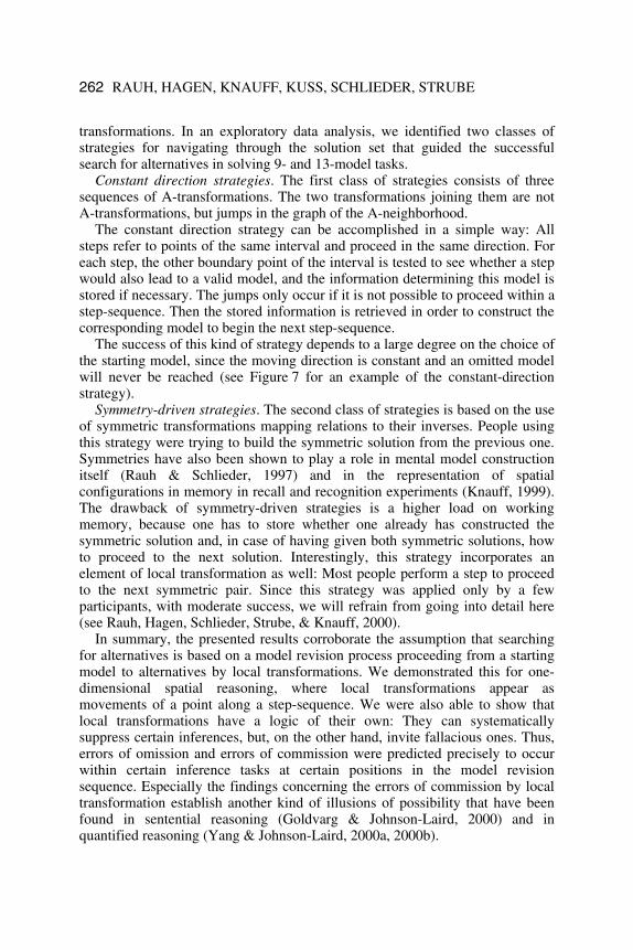
The success of this kind of strategy depends to a large degree on the choice of the starting model, since the moving direction is constant and an omitted model will never be reached (see Figure 7 for an example of the constant-direction strategy).

Symmetry-driven strategies. The second class of strategies is based on the use of symmetric transformations mapping relations to their inverses. People using this strategy were trying to build the symmetric solution from the previous one. Symmetries have also been shown to play a role in mental model construction itself (Rauh & Schlieder, 1997) and in the representation of spatial configurations in memory in recall and recognition experiments (Knauff, 1999). The drawback of symmetry-driven strategies is a higher load on working memory, because one has to store whether one already has constructed the symmetric solution and, in case of having given both symmetric solutions, how to proceed to the next solution. Interestingly, this strategy incorporates an element of local transformation as well: Most people perform a step to proceed to the next symmetric pair. Since this strategy was applied only by a few participants, with moderate success, we will refrain from going into detail here (see Rauh, Hagen, Schlieder, Strube, & Knauff, 2000).

In summary, the presented results corroborate the assumption that searching for alternatives is based on a model revision process proceeding from a starting model to alternatives by local transformations. We demonstrated this for one-dimensional spatial reasoning, where local transformations appear as movements of a point along a step-sequence. We were also able to show that local transformations have a logic of their own: They can systematically suppress certain inferences, but, on the other hand, invite fallacious ones. Thus, errors of omission and errors of commission were predicted precisely to occur within certain inference tasks at certain positions in the model revision sequence. Especially the findings concerning the errors of commission by local transformation establish another kind of illusions of possibility that have been found in sentential reasoning (Goldvarg & Johnson-Laird, 2000) and in quantified reasoning (Yang & Johnson-Laird, 2000a, 2000b).


Experiment 4: Availability of Alternative Models

Experiment 3 shows that people generate a starting model of the premises and then generate alternatives by locally transforming it. To provide additional empirical support for this idea, there should also be effects in a verification task with indeterminate three-term series problems: There should be (i) increasing verification latencies for alternatives that have a higher rank in the generation order, and (ii) the number of errors should also increase with alternatives with higher generation rank. The following experiment tests these hypotheses.

Method Participants. Fifty-two students from the University of Freiburg, 26 female

and 26 male with an age range from 20 to 38 years, were paid for participation or fulfilled course requirements. They had no formal training in logic, and they had not previously participated in an experiment on reasoning.

Materials. As already noted it is reasonable to only investigate the 3-model tasks and the 5-model tasks, respectively. With these tasks, one can expect a considerable number of observations along the generation sequence (no bottom effect), that are not affected by generation strategies as in the case of tasks with 9 or 13 models. Out of these 66 3-model and 5-model tasks, we selected those three-term series problems where the generated sequences in Experiment 3 were most concordant: These were the three-term series problems “di – f” and “mi – s” (3 model cases), and “oi – <” and “> – d” (5 model cases). We also added

Figure 7. Model revision with the constant direction strategy for the 13-model task (> - <). Instead of changing the moving endpoint of interval Z in (5) to the start point and thus changing direction from (8) to (7), participants prefer to make a non-local transformation from (5) to (6), in order to keep the direction of moving points constant. Another non-local transformation has to be made between (8) and (9).


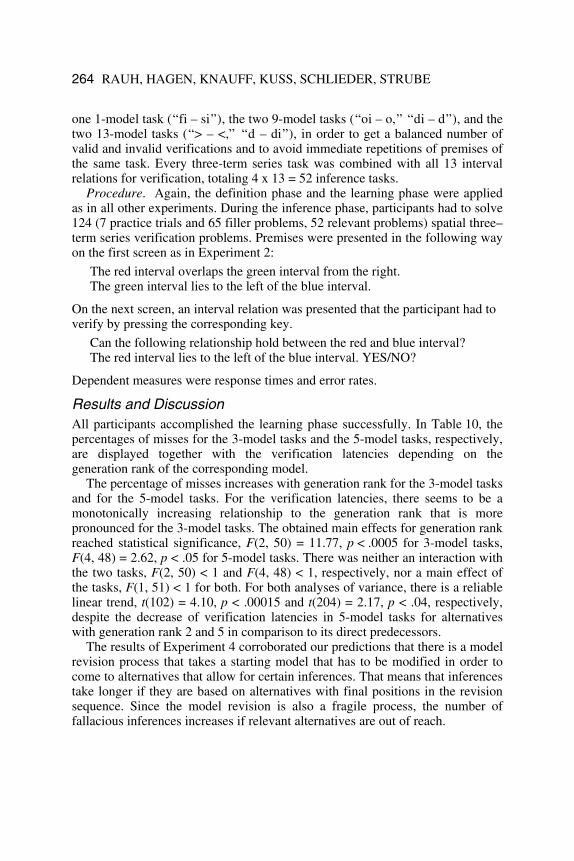
one 1-model task (“fi – si”), the two 9-model tasks (“oi – o,” “di – d”), and the two 13-model tasks (“> – <,” “d – di”), in order to get a balanced number of valid and invalid verifications and to avoid immediate repetitions of premises of the same task. Every three-term series task was combined with all 13 interval relations for verification, totaling 4 x 13 = 52 inference tasks.

Procedure. Again, the definition phase and the learning phase were applied as in all other experiments. During the inference phase, participants had to solve 124 (7 practice trials and 65 filler problems, 52 relevant problems) spatial three–term series verification problems. Premises were presented in the following way on the first screen as in Experiment 2:

The red interval overlaps the green interval from the right. The green interval lies to the left of the blue interval.

On the next screen, an interval relation was presented that the participant had to verify by pressing the corresponding key.

Can the following relationship hold between the red and blue interval? The red interval lies to the left of the blue interval. YES/NO?

Dependent measures were response times and error rates.

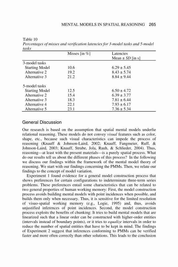
Results and Discussion All participants accomplished the learning phase successfully. In Table 10, the percentages of misses for the 3-model tasks and the 5-model tasks, respectively, are displayed together with the verification latencies depending on the generation rank of the corresponding model.

The percentage of misses increases with generation rank for the 3-model tasks and for the 5-model tasks. For the verification latencies, there seems to be a monotonically increasing relationship to the generation rank that is more pronounced for the 3-model tasks. The obtained main effects for generation rank reached statistical significance, F(2, 50) = 11.77, p < .0005 for 3-model tasks, F(4, 48) = 2.62, p < .05 for 5-model tasks. There was neither an interaction with the two tasks, F(2, 50) < 1 and F(4, 48) < 1, respectively, nor a main effect of the tasks, F(1, 51) < 1 for both. For both analyses of variance, there is a reliable linear trend, t(102) = 4.10, p < .00015 and t(204) = 2.17, p < .04, respectively, despite the decrease of verification latencies in 5-model tasks for alternatives with generation rank 2 and 5 in comparison to its direct predecessors.

The results of Experiment 4 corroborated our predictions that there is a model revision process that takes a starting model that has to be modified in order to come to alternatives that allow for certain inferences. That means that inferences take longer if they are based on alternatives with final positions in the revision sequence. Since the model revision is also a fragile process, the number of fallacious inferences increases if relevant alternatives are out of reach.


General Discussion

Our research is based on the assumption that spatial mental models underlie relational reasoning. These models do not convey visual features such as color, shape, etc., because such visual characteristics can impede the process of reasoning (Knauff & Johnson-Laird, 2002; Knauff, Fangmeier, Ruff, & Johnson-Laird, 2003; Knauff, Strube, Jola, Rauh, & Schlieder, 2004). Thus, reasoning—at least with the present materials—is a purely spatial process. What do our results tell us about the different phases of this process? In the following we discuss our findings within the framework of the mental model theory of reasoning. We start with our findings concerning the PMMs. Then, we relate our findings to the concept of model variation.

Experiment 1 found evidence for a general model construction process that shows preferences for certain configurations to indeterminate three-term series problems. These preferences entail some characteristics that can be related to two general properties of human working memory: First, the model construction process avoids building mental models with point incidences when possible, and builds them only when necessary. Thus, it is sensitive for the limited resolution of visuo-spatial working memory (e.g., Logie, 1995) and, thus, avoids unjustified inferences of point incidences. Second, the model construction process exploits the benefits of chunking: It tries to build mental models that are linearized such that a linear order can be constructed with higher-order entities (intervals instead of boundary points), or it tries to equalize intervals in order to reduce the number of spatial entities that have to be kept in mind. The findings of Experiment 2 suggest that inferences conforming to PMMs can be verified faster and more often correctly than other solutions. This leads to the conclusion

Table 10 Percentages of misses and verification latencies for 3-model tasks and 5-model tasks Misses [in %] Latencies

Mean ± SD [in s] 3-model tasks Starting Model 10.6 6.29 ± 5.45 Alternative 2 19.2 8.43 ± 5.74 Alternative 3 21.2 8.84 ± 9.44 5-model tasks Starting Model 12.5 6.50 ± 4.72 Alternative 2 15.4 6.39 ± 3.77 Alternative 3 18.3 7.81 ± 6.44 Alternative 4 22.1 7.93 ± 6.17 Alternative 5 23.1 7.36 ± 5.34


that in spatial relational inference, solutions to indeterminate three-term series problems are processed in a serial manner.

In Part II, two further experiments were conducted to clarify the third phase of inference from mental model theory: Are alternatives constructed by an iterative construction process, or rather by model revision? The results of Experiment 3 support the assumption of a general revision process that takes the PMM as input and locally transforms it to come to the next alternative. An interesting fact arises from this process. Since the revision process operates on an integrated representation of the state of affairs the premises describe, it has a logic of its own. Two systematic inferential biases can be explained by this assumption: Errors of omission occur if local transformations are more demanding (change of direction, change of moving points). This is in accordance with the well-known effect from the mental models literature that reasoners make fallacious conclusions because they fail to consider all possible models. However, we can predict which models are more prone to be ignored: These are those mental models that rest beyond more demanding local transformations.

The second type of inferential bias is even more interesting since according to mental model theory it should not occur, namely that reasoners build mental models that are no longer models of the premises. These errors of commission are provoked if local transformations supply an alternative that accidentally violates one or more premise. Additional information has to be provided if such non-solutions have to be barred from coming to mind. Mental model theory assumes a kind of mental footnote that could do this job and inform the model revision process if premise information gets violated. Unfortunately, mental footnotes may be quickly forgotten, as evidence from other studies of reasoning shows (Johnson-Laird & Savary, 1995). Thus, these errors of commission may occur more often than presumed. The notion of a model revision process could further be corroborated in Experiment 4: The verification of inferences is monotonically related to the position of a corresponding model in the revision sequence. This relationship was found with respect to accuracy data in a perfect manner, and to a lesser extent with verification latencies.

The findings of all four experiments went into a process model that constructs PMMs and revises them in a manner similar to that used by our participants (Schlieder et al., 2002). Thus, it gives a detailed account for spatial reasoning and offers new theoretical concepts like model revision and local transformation that might be fruitful in other areas of reasoning as well.

Acknowledgments

This research was supported by the Deutsche Forschungsgemeinschaft (DFG) under contract numbers Str 301/5-1, Str 301/5-2, and in the Transregional Collaborative Research Center Spatial Cognition (SFB/TR8; http://www.sfbtr8.uni-bremen.de). MK is supported by a Heisenberg-Award from the DFG. We would like to thank Goran Sunjka for his extensive help in


implementing the computer-assisted Experiment 3, Katrin Balke and Kristina Kirn for running the experiments, Kristen Drake for proofreading an earlier draft, and Marco Ragni and four anonymous reviewers for many useful comments on the manuscript.

References

Allen, J. F. (1983). Maintaining knowledge about temporal intervals. Commun-ications of the ACM, 26, 832–843.

Anderson, J. R. (2000). Cognitive psychology and its implications (5th ed.). New York: Worth Publishers.

Bell, V., & Johnson-Laird, P. N. (1998) A model theory of modal reasoning. Cognitive Science, 22, 25–51.

Berendt, B. (1996). Explaining preferred mental models in Allen inferences with a metrical model of imagery. In G. W. Cottrell (Ed.), Proceedings of the Eighteenth Annual Conference of the Cognitive Science Societey (pp. 489–494). Mahwah, NJ: Lawrence Erlbaum Associates.

Borning, A., Lin, R., & Marriott, K. (1997). Constraints for the Web. Proceedings of the Fifth ACM International Multimedia Conference, 173–182.

Borning, A., Lin, R., & Marriott, K. (2000). Constraint-based document layout for the Web. Multimedia Systems, 8, 177–189.

Bucciarelli, M., & Johnson-Laird, P. N. (1999). Strategies in syllogistic reasoning. Cognitive Science, 23, 247–303.

Byrne, R. M. J., & Johnson-Laird, P. N. (1989). Spatial reasoning. Journal of Memory and Language, 28, 564–575.

Cohn, A. G., & Hazarika, S. M. (2001). Qualitative spatial representation and reasoning: An overview. Fundamenta Informaticae, 46, 1–29.

Ehrlich, K., & Johnson-Laird, P. N. (1982). Spatial descriptions and referential continuity. Journal of Verbal Learning and Verbal Behavior, 21, 296–306.

Evans, J. St. B. T. (1972). On the problem of interpreting reasoning data: Logical and psychological approaches. Cognition, 1, 373–384.

Freksa, C. (1991). Qualitative spatial reasoning. In D. M. Mark & A. U. Frank (Eds.), Cognitive and linguistic aspects of geographic space (pp. 361–372). Dordrecht: Kluwer Academic Publishers.

Freksa, C. (1992). Temporal reasoning based on semi-intervals. Artificial Intelligence, 54, 199–227.

Goldvarg, Y., & Johnson-Laird, P. N. (2000). Illusions in modal reasoning. Memory & Cognition, 28, 282–294.

Johnson-Laird, P. N. (1972). The three-term series problem. Cognition, 1, 57–82.

Johnson-Laird, P. N. (1983). Mental models. Towards a cognitive science of language, inference, and consciousness. Cambridge, MA: Harvard University Press.


Johnson-Laird, P. N. (2001). Mental models and deduction. Trends in Cognitive Sciences, 5, 434–442.

Johnson-Laird, P. N., & Byrne, R. M. J. (1991). Deduction. Hove(UK): Erlbaum.

Johnson-Laird, P. N., & Savary, F. (1995). How to make the impossible seem probable. In J. D. Moore & J. F. Lehman (Eds.), Proceedings of the Seventeenth Annual Conference of the Cognitive Science Society (pp. 381–384). Mahwah, NJ: Lawrence Erlbaum Associates.

Knauff, M. (1999). The cognitive adequacy of Allen's interval calculus for qualitative spatial representation and reasoning. Spatial Cognition and Computation, 1, 261–290.

Knauff, M., Fangmeier, T., Ruff, C. C., & Johnson-Laird, P. N. (2003). Reasoning, models, and images: Behavioral measures and cortical activity. Journal of Cognitive Neuroscience, 15, 559–573.

Knauff, M., & Johnson-Laird, P. N. (2002). Visual imagery can impede reasoning. Memory & Cognition, 30, 363–371.

Knauff, M., Rauh, R., & Schlieder, C. (1995). Preferred mental models in qualitative spatial reasoning: A cognitive assessment of Allen's calculus. In J. D. Moore & J. F. Lehman (Eds.), Proceedings of the Seventeenth Annual Conference of the Cognitive Science Society (pp. 200–205). Mahwah, NJ: Lawrence Erlbaum Associates.

Knauff, M., Strube, G., Jola, C., Rauh, R., & Schlieder, C. (2004). The psychological validity of qualitative spatial reasoning in one dimension. Spatial Cognition and Computation, 4, 167–188.

Kolodner, J. L. (1993). Case-based reasoning. San Mateo, CA: Morgan Kaufmann Publishers.

Ligozat, G. (1990). Weak representations of interval algebras. In Proceedings of the Eighth National Conference on Artificial Intelligence (Vol. 2, pp. 715–720). Menlo Park, CA: AAAI Press / The MIT Press.

Logie, R. H. (1995). Visuo-spatial working memory. Hove(UK): Erlbaum. Longley, P. A., Goodchild, M. F., Maguire, D. J., & Rhind, D. W. (2001).

Geographic information systems and science. New York: John Wiley & Sons. Mani, K., & Johnson-Laird, P. N. (1982). The mental representation of spatial

descriptions. Memory & Cognition, 10, 181–187. Nebel, B., & Bürckert, H. -J. (1994). Reasoning about temporal relations: A

maximal tractable subclass of Allen's interval algebra. In Proceedings of the Twelfth National Conference on Artificial Intelligence (Vol. 1, pp. 356–361). Menlo Park, CA: AAAI Press / MIT Press.

Rauh, R. (2000). Strategies of constructing preferred mental models in spatial relational inference. In W. Schaeken, G. De Vooght, A. Vandierendonck, & G. d'Ydewalle (Eds.), Deductive reasoning and strategies (pp. 177–190). Mahwah, NJ: Lawrence Erlbaum Associates.


Rauh, R., Hagen, C., Schlieder, C., Strube, G., & Knauff, M. (2000). Searching for alternatives in spatial reasoning: Local transformations and beyond. In L. R. Gleitman & A. K. Joshi (Eds.), Proceedings of the Twenty Second Annual Conference of the Cognitive Science Society (pp. 871–876). Mahwah, NJ: Lawrence Erlbaum Associates.

Rauh, R., & Schlieder, C. (1997). Symmetries of model construction in spatial relational inference. In M. G. Shafto & P. Langley (Eds.), Proceedings of the Nineteenth Annual Conference of the Cognitive Science Society (pp. 638–643). Mahwah, NJ: Lawrence Erlbaum Associates.

Schlieder, C. (1998). Diagrammatic transformation processes on two-dimensional relational maps. Journal of Visual Languages and Computing, 9, 45–59.

Schlieder, C. (1999). The construction of preferred mental models in reasoning with interval relations. In G. Rickheit & C. Habel (Eds.), Mental models in discourse processing and reasoning (pp. 333–357). Amsterdam: Elsevier Science Publishers.

Schlieder, C., & Berendt, B. (1998). Mental model construction in spatial reasoning: A comparison of two computational theories. In U. Schmid, Krems, J. F., & F. Wysotzki (Eds.), Mind modelling: A cognitive science approach to reasoning, learning and discovery (pp. 133–162). Lengerich (Germany): Pabst Science Publishers.

Schlieder, C., & Hagen, C. (2000). Interactive layout generation with a diagrammatic constraint language. In C. Freksa, W. Brauer, C. Habel, & K. F. Wender (Eds.), Spatial cognition II. Integrating abstract theories, empirical studies, formal methods, and practical applications (pp. 198–211). Berlin: Springer.

Schlieder, C., Hagen, C., Eijkel, D. v. d., Knauff, M., Rauh, R., & Strube, G. (2002). A cognitive modelling of mental models in qualitative spatial reasoning. Retrieved February 28, 2004, from http://www.iig.uni-freiburg.de/cognition/members/hagen/demo/mm01.html

Tversky, A., & Kahneman, D. (1974). Judgment under uncertainty: Heuristics and biases. Science, 185, 1124–1131.

Williams, E. J. (1949). Experimental designs balanced for the estimation of residual effects of treatments. Australian Journal of Scientific Research. Series A - Physical Sciences, 2, 149–168.

Yang, Y., & Johnson-Laird, P. N. (2000a). How to eliminate illusions in quantified reasoning. Memory & Cognition, 28, 1050–1059.

Yang, Y., & Johnson-Laird, P. N. (2000b). Illusions in quantified reasoning: How to make the impossible seem possible, and vice versa. Memory & Cognition, 28, 452–465.

preferred and alternative mental models in spatial reasoning · reasoning, and syllogistic...

Documents