prelauncii forecasting of new automobiles: models and...
TRANSCRIPT
PRELAUNCII FORECASTING OF NEW AUTOMOBILES:MODELS AND IMPLEMENTATION
by
Glen L. Urban*John R. Hauser**John H. Roberts***
Working Paper #1820-86Revised September 1988
Deputy Dean and Dai-Ichi Kangyo Bank Professor of Management,School of Management, M.I.T., Cambridge, MA 02139
Professor of Management Science,School of Management, M.I.T., Cambridge, MA 02139
*** Associate Professor of Management Science,University of New South Wales, Kensington, NSW 2033, Australia

PRELAUNCH FORECASTING OF NEW AUTOMOBILES:MODELS AND IMPLEMENTATION
ABSTRACT
As a first step towards a better understanding of durable goods
marketing, a prelaunch forecasting model and measurement system for marketing
planning is proposed and applied to a new automobile. Especially
challenging factors included in the model are: active search by consumers,
dealer visits, word-of-mouth communication, magazine reviews, and production
constraints. We describe the managerial situation, sampling scheme, consumer
measurement, and initial analysis. We develop a detailed consumer flow model
indicating the detailed modeling of key customer transitions and
illustrating how data, previous experience, judgment, and fitting are used to
"calibrate" the model to fit the sales history of a control car. After
indicating how the model was used to evaluate marketing strategies we compare
the model's predictions to actual sales of the new automobile. We close with
short descriptions of subsequent applications and a discussion of the
challenges that remain.

1
Consumer durable goods purchases (e.g., appliances, autos, cameras)
represent a huge market, but relatively few management science models have
been successfully implemented in this area of business. In this paper we
attack the marketing problems of a subset of the durables market --
automobiles -- in an effort to understand the challenging issues in
marketing durables and how they can be modeled.
Our purpose is to describe a model and measurement system developed for
and used by the automobile industry managers. The system forecasts the
life-cycle of a new car before introduction and develops improved
introductory strategies. Such models are applied widely in frequently
purchased consumer goods markets based on test marketing (see Urban and
Hauser, 1980, pp. 429-47 for a review) and on pre-test market measures (e.g.,
Silk and Urban, 1978; Pringle, Wilson, and Brody, 1982; and Urban and Hauser,
1980, pp. 386-411). But standard models must be modified for premarket
forecasting of new consumer durable goods such as an automobile.
We modify existing Markov and choice structures to build a model that
can encompass unique aspects of durable goods (automobiles) and which can be
implemented. After briefly highlighting some important modeling challenges
in applications to autos, we describe two modeling approaches to forecasting
the launch of a new model car offered by General Motors. We show how a
simple index model evolves to a detailed consumer flow model in order to
provide analyses to support key managerial decisions. We compare 18 months
of actual market data to the forecasted values and discuss the implications
of our work for forecasting sales of other new durable goods.

2
The focus of this paper is the application. We extend existing models
for production constraints and measure customer reactions after conditional
information that simulates word-of-mouth and trade press input; but our
emphasis is on how state-of-the-art marketing science models can be used to
affect major managerial decisions.
CHALLENGES IN MODELING AUTOMOBILES
Automobiles represent a very large market; sales in the 1988 model year
were over 100 billion dollars in the U.S. and over 300 billion world wide. A
new car can contribute over one billion dollars per year in sales if it
sells a rather modest 100,000 units per year at an average price of $12,000
per car. Major successes can generate several times this in sales and
associated profits.
These potential rewards encourage firms to allocate large amounts of
capital to design, production, and selling of a new model. Ford spent three
billion dollars developing the Taurus/Sable line (Mitchell 1986). General
Motors routinely spends one billion dollars on a new model such as the Buick
Electra. Most of this investment occurs before launch; if the car is not a
market success, significant losses result.
Rates of failure are not published for the auto industry, but many cars
have fallen short of expectations. Most failures are not as dramatic as the
Edsel which was withdrawn from the market, but significant losses occur in
two ways. When sales are below forecasts there is excess production capacity
and inventories. In this case, capital costs are excessive and prices must
be discounted or other marketing actions undertaken to clear inventories.
Losses also occur when the forecast of sales is below the market demand. In
this case not enough cars can be produced, inventories are low, and prices
III

3
are firm. The car is apparently very profitable, but a large opportunity
cost may be incurred. Profits could have been higher if the forecast had
been more accurate and more production capacity had been planned.
For those readers unfamiliar with the automobile industry we describe a
few facts that will become important in our application.
Consumer Response
Search and experience. In automobiles, consumers reduce risk by
searching for information and, in particular, visit showrooms. Typically 75
percent of buyers test drive one or more cars. The marketing manager's task
is to convince the consumer to consider the automobile, get the prospect into
the showroom, and facilitate purchasing with test drives and personal selling
efforts.
Word-of-Mouth Communication/Magazine Reviews. One source of information
about automobiles is other consumers. Another is independent magazine
reviews such as Consumer Reports and Car and Driver. Given the thousands of
dollars involved in buying a car, the impact of these sources is quite large.
Importance of availability. Eighty percent of domestic sales are "off
the lot," i.e., purchased from dealer's inventory. Many consumers will
consider alternative makes and models if they cannot find a car with the
specific features, options, and colors they want.
Managerial Issues
No test market. Building enough cars for test marketing (say, 1,000
cars) requires a full production line that could produce 75,000 units. Once
this investment is made, the "bricks and mortar" are in place for a national
launch and the major element of risk has been borne.
4
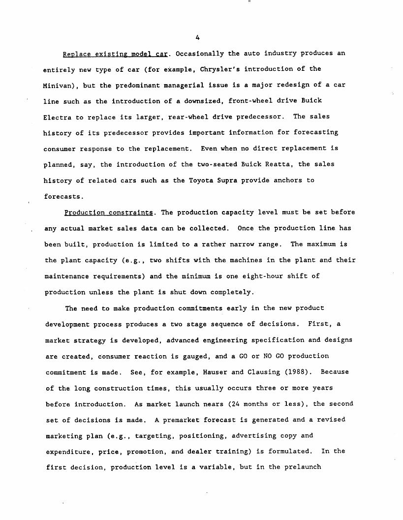
Replace existing model car. Occasionally the auto industry produces an
entirely new type of car (for example, Chrysler's introduction of the
Minivan), but the predominant managerial issue is a major redesign of a car
line such as the introduction of a downsized, front-wheel drive Buick
Electra to replace its larger, rear-wheel drive predecessor. The sales
history of its predecessor provides important information for forecasting
consumer response to the replacement. Even when no direct replacement is
planned, say, the introduction of the two-seated Buick Reatta, the sales
history of related cars such as the Toyota Supra provide anchors to
forecasts.
Production constraints. The production capacity level must be set before
any actual market sales data can be collected. Once the production line has
been built, production is limited to a rather narrow range. The maximum is
the plant capacity (e.g., two shifts with the machines in the plant and their
maintenance requirements) and the minimum is one eight-hour shift of
production unless the plant is shut down completely.
The need to make production commitments early in the new product
development process produces a two stage sequence of decisions. First, a
market strategy is developed, advanced engineering specification and designs
are created, consumer reaction is gauged, and a GO or NO GO production
commitment is made. See, for example, Hauser and Clausing (1988). Because
of the long construction times, this usually occurs three or more years
before introduction. As market launch nears (24 months or less), the second
set of decisions is made. A premarket forecast is generated and a revised
marketing plan (e.g., targeting, positioning, advertising copy and
expenditure, price, promotion, and dealer training) is formulated. In the
first decision, production level is a variable, but in the prelaunch
11

5
forecasting phase (the focus of this paper) the capacity constraints are
taken as given.
"Price" forecasting problem. Production capacity is based on the best
information available at the time, but as engineering and manufacturing
develop the prototype cars, details change as do external conditions in the
economy. At the planned price and marketing levels consumers may wish to
purchase more or fewer vehicles than will be produced. The number of
vehicles that would be sold if there were no production constraints is known
as "free expression." Naturally, free expression is pegged to a price and
marketing effort.
If the free expression demand at a given level of price and marketing
effort is less than the production minimum, the company and its dealers must
find a way to sell more cars (e.g., change price, promotion, dealer
incentives, advertising, or targeting new markets). If the forecast is in
the range, marketing variables can be used to maximize profit with little
constraint. If free expression demand is above the maximum production, then
opportunities exist to increase profit by adjusting price, reducing
advertising, or by producing cars with many optional features.
EXISTING LITERATURE AND INDUSTRY PRACTICE
Marketing Science
Marketing science has a rich tradition of life cycle diffusion models
which describe durable good sales via phenomena such as innovators,
imitators, and the diffusion of innovation. These models focus on major
innovations such as color TV or computer memory (Bass 1969, Robinson and
Lakani 1975, Mahajan and Muller 1979, Jeuland 1981, Horsky and Simon 1983,
Kalish 1985, and Wind and Mahajan 1986). However, for forecasting, these

6
models require substantial experience with national sales (Heeler and Hustad
1980). In prelaunch analysis no national sales history is available for the
new auto model. Thus, the initial penetration, diffusion parameter, and
total sales over the life cycle would need to be set based on judgment,
market research, or analogy to other product categories. In our application
we incorporate these "data" sources, but in a model adapted to the details of
consumer response and the managerial situation in the automobile industry.
One model of individual multiattribute utility, risk, and belief
dynamics has been proposed for use in prelaunch forecasting of durables
(Roberts and Urban 1988). This model can be parametized based on market
research before launch, but our experience with this complex model suggests
that it is difficult to implement and does not deal with production
constraints and the "price" forecasting problem.
Industry Practice
Industry practice has included market research to obtain consumer
response to new durables. In the auto industry concept tests, focus groups,
perceptual mapping, conjoint analysis, and consumer "clinics" have been
utilized. The clinics traditionally collect likes, dislikes, and buying
intent with respect to currently available cars. After exposure to a fiber-
glass mockup of a new car in a showroom setting, free-expression
"diversion" from the consumer's most preferred currently-available model is
measured. (That is, consumers indicate which make and model car they would
have purchased. The clinics measure the percentage of these consumers who
would now purchase the new car.)
Ill
7
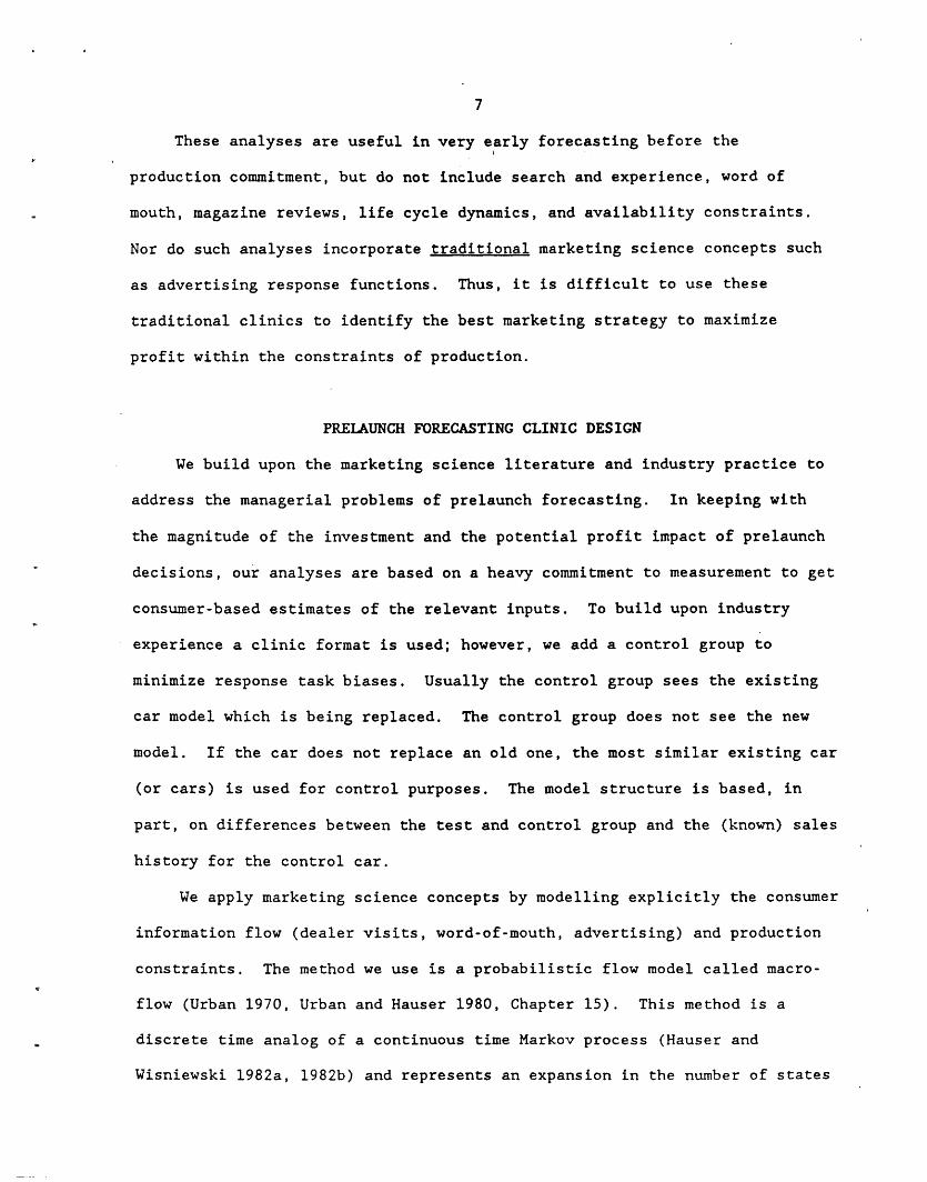
These analyses are useful in very early forecasting before the
production commitment, but do not include search and experience, word of
mouth, magazine reviews, life cycle dynamics, and availability constraints.
Nor do such analyses incorporate traditional marketing science concepts such
as advertising response functions. Thus, it is difficult to use these
traditional clinics to identify the best marketing strategy to maximize
profit within the constraints of production.
PRELAUNCH FORECASTING CLINIC DESIGN
We build upon the marketing science literature and industry practice to
address the managerial problems of prelaunch forecasting. In keeping with
the magnitude of the investment and the potential profit impact of prelaunch
decisions, our analyses are based on a heavy commitment to measurement to get
consumer-based estimates of the relevant inputs. To build upon industry
experience a clinic format is used; however, we add a control group to
minimize response task biases. Usually the control group sees the existing
car model which is being replaced. The control group does not see the new
model. If the car does not replace an old one, the most similar existing car
(or cars) is used for control purposes. The model structure is based, in
part, on differences between the test and control group and the (known) sales
history for the control car.
We apply marketing science concepts by modelling explicitly the consumer
information flow (dealer visits, word-of-mouth, advertising) and production
constraints. The method we use is a probabilistic flow model called macro-
flow (Urban 1970, Urban and Hauser 1980, Chapter 15). This method is a
discrete time analog of a continuous time Markov process (Hauser and
Wisniewski 1982a, 1982b) and represents an expansion in the number of states
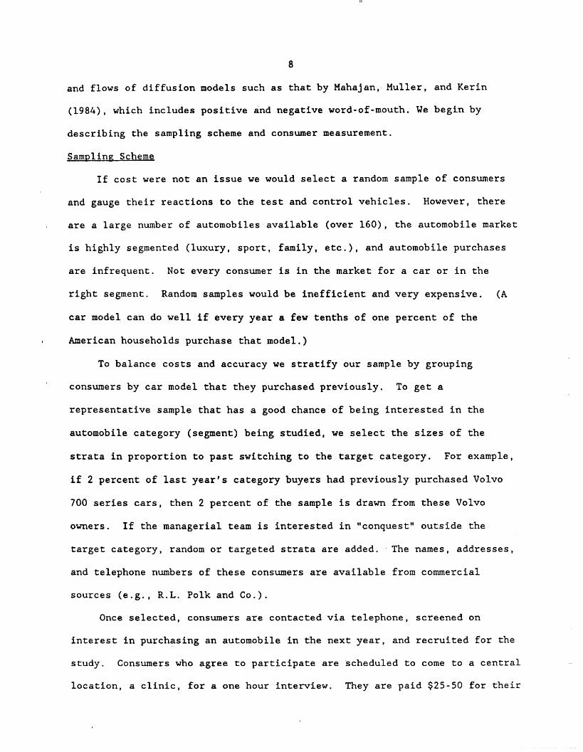
8
and flows of diffusion models such as that by Mahajan,. Muller, and Kerin
(1984), which includes positive and negative word-of-mouth. We begin by
describing the sampling scheme and consumer measurement.
Sampling Scheme
If cost were not an issue we would select a random sample of consumers
and gauge their reactions to the test and control vehicles. However, there
are a large number of automobiles available (over 160), the automobile market
is highly segmented (luxury, sport, family, etc.), and automobile purchases
are infrequent. Not every consumer is in the market for a car or in the
right segment. Random samples would be inefficient and very expensive. (A
car model can do well if every year a few tenths of one percent of the
American households purchase that model.)
To balance costs and accuracy we stratify our sample by grouping
consumers by car model that they purchased previously. To get a
representative sample that has a good chance of being interested in the
automobile category (segment) being studied, we select the sizes of the
strata in proportion to past switching to the target category. For example,
if 2 percent of last year's category buyers had previously purchased Volvo
700 series cars, then 2 percent of the sample is drawn from these Volvo
owners. If the managerial team is interested in "conquest" outside the
target category, random or targeted strata are added. The names, addresses,
and telephone numbers of these consumers are available from commercial
sources (e.g., R.L. Polk and Co.).
Once selected, consumers are contacted via telephone, screened on
interest in purchasing an automobile in the next year, and recruited for the
study. Consumers who agree to participate are scheduled to come to a central
location, a clinic, for a one hour interview. They are paid $25-50 for their
11

9
participation. If both spouses participate in the decision to buy a new car,
both are encouraged to come.
Basic Clinic Design
Upon arrival two-thirds of the consumers are assigned randomly to the
test car group and one-third to the control car group. In both cases they
are told they are evaluating next year's models. (This is believable to
consumers because most year-to-year changes in an automobile model are
relatively minor.) (See Figure 1 for the basic measurement design.)
<Insert Figure One, 'Experimental Design...,' about here>.
After warmup and screening questions, the consumer(s) is asked to
describe car(s) that he (she or they) now own, including make, model, year,
miles per gallon (if known), options, maintenance costs, etc. This task puts
them in a frame of mind to evaluate cars and provides valuable background
information.
They are next presented with a list of the 160 or so automobile lines
available, along with abridged information on price (base and "loaded" with
options), fuel economy and engine size, and asked to indicate which
automobiles they would consider seriously. The modal consideration set
consists of about three cars; the median is five cars. In addition, they
indicate the cars they feel would be their first, second, and if
appropriate, third choices. They rate these cars on subjective probability
scales (Juster 1966) and on a constant sum paired comparison of preferences
across their first three auto choices. These questions allow us to estimate
10
"diversion," the percent of consumers who intended to purchase another car
who will now purchase the target car.
Now the experimental treatments begin. Two-thirds of the consumers are
shown concept boards (or rough ad copy) for the test car in an effort to
simulate advertising exposure. One-third are shown concept boards for the
control car. They rate the concept on the same probability and preference
scales as the cars they now own.
In the market, after advertising exposure, some consumers will visit
showrooms for more information, others will seek word-of-mouth or magazine
evaluations. Thus, as shown in Figure 1, the sample is split. One half of
each test/control treatment cell sees video tapes which simulate word-of-
mouth 1 and evaluations which represent consumer magazine evaluations (e.g.,
Consumer Reports); the other half are allowed to test-drive the car to which
they are assigned. The video treatment is divided into positive and negative
exposure cells. Probability and constant sum paired comparison preference
measures are taken for the stimulus car and the respondents' top three
choices among cars now on the market. The half which saw the videotapes and
magazine abstracts now test drives the car; the half which test drove is now
exposed to the videotape and magazine information. Again probability and
preference measures are taken. More elaborate designs can be used. For
example, management needs may require splitting the sample further on two-
1 The videotapes include a commentator and three consumers.Professional actors are used, but an attempt is made to match thedemographics of the target market. The semantics come from earlier focusgroups on prototypes of the car being tested. One script is positive in itscontent and another is negative. Both use the same actors. The magazineexposure is a mock-up from the fictitious "Consumer laboratories, Inc." andput in a format similar to Consumer Reports. The quantitative evaluationsare chosen to match the qualitative video tapes. We have found throughpretesting that consumers find the videotapes and magazine reports believableand realistic.
III

11
door vs. four-door or adding measurement modules for consuner budget planning
and/or conjoint analysis with respect to potential feature variations. It is
also possible to split on alternative positioning strategies. All such
options in the experimental design require tradeoffs with respect to sample
size and length of interview. In the application we are describing, the
design in Figure 1 was used.
A NEW MID-SIZED CAR--PHASE I ANALYSIS
This application takes place in the Buick Division of General Motors.
General Motors had made a strategic decision to downsize all of its luxury
cars -- its 1983 Electra/Park Avenue had been launched. In the fall of 1984,
eighteen months prior to launch, we began analysis of the next downsized car
-- the division's largest selling mid-sized model. Sales targets were set
optimistically at 450,000 units -- a 15 percent share of the mid-sized
market. This represented doubling of current sales volume and a fifty
percent increase in market share.
The clinic was run in Atlanta, Georgia. The sample size was 534 and
drawn randomly from car registration data but stratified by current
ownership: 119 from previous buyers of the target car, 139 from previous
buyers of other cars from the division, 128 from other domestic cars, and 148
from imports.
Top-line Analysis
In 1970, Little studied how managers react to marketing science models.
In that seminal article he proposed a "decision calculus," a set of
guidelines marketing models should follow to be accepted and used.
A tenant of his proposal was that managers want models they can trust,
which match their intuitions, and which are readily understandable. In the

12
late 1980s managers have the same needs. Thus, before we introduce the more
complex analysis with its probabilistic modeling of consumer information
flow, we describe top-line diagnostic information from the clinic and an
initial forecast based on an index model.
Our first diagnostic indicator is relative preference. Recall that the
consumers rated three currently available cars plus the new car (or, for the
2control group, the existing car) on constant paired comparisons. One
indicator of relative preference is the preference value of the new car
divided by the sum of existing and new cars. Another measure is the percent
of consumers who rate the new car higher than the existing cars. We have
found both measures give similar results, thus Table 1 reports only the
relative measure. The test/control design is critical here. Exposure to
concepts can be inflated (deflated) due to the specifics of the task, but
such inflation should be constant across test or control. Thus, although
each specific measure may be inflated, their ratio should be unbiased.
<Insert Table 1, "Relative Preference...," about here.>
Table 1 was a disappointment to management. Although not all
differences were significant, all test car values were below the control. It
was clear that the test car would not do as well in terms of preference as
the rear-wheel drive car it was scheduled to replace.
Furthermore, relative values of preference decrease when consumers have
more information. They decrease from a ratio of .94 for concept only
exposure to .88 for concept and positive word-of-mouth (wom) and magazine
exposure, .87 for concept and drive, and .84 for full positive information
2 A few consumers rated only two cars because that is all they considered.
III

13
(The latter the is average of ratios of concept/exposure to drive and to
positive word-of-mouth and magazine exposure in either order: (.78 +
.90)/2). A doubling of sales volume did not look promising.
At this point it became important for managers to obtain a "ballpark"
estimate of the potential sales shortfall. If it was sufficiently large,
they would have to consider radical strategies. To obtain top-line,
"ballpark" forecasts, we developed an index model similar to those used by
Little (1975, 1979) and Urban (1968).
Top-line Forecasts
In an index model we modify a base sales level, in this case the sales
history of the control car, by a series of percentage indices. From previous
research (Silverman 1982), we knew that the sales pattern for mid-sized car
models followed a four to five year "life-cycle" which had an inverted U-
shape. Not until a sufficiently novel relaunch did the life-cycle restart.
In this case management felt the new front-wheel drive car would restart the
life-cycle and that the pattern, but not the magnitude, would be similar to
the rear-wheel drive car.
Management felt that the sales of the new car t years after its
introduction, S(t), would follow the pattern of the sales history of the
control car, Sc(t) if all else were equal. We would modify this forecast by
factors due to preference, P(t) (defined as the ratio of preference of the
new car to the control car) as measured in the clinic; industry volume, V(t)
as estimated by exogenous econometric models; and competitive intensity, C(t)
(nominally 1.0 if no new competition enters and less than one when new
competitive cars enter) as judged by the managers. (In other applications
further indices are added as the situation demands.)
14
In symbols, the top-line forecast is given by:
(1) S(t) - Sc(t)*P(t)*V(t)*C(t)
The preference index was based on the clinic measures. Because
information reaches consumers over the life-cycle, and because the preference
ratios decrease in Table 1 as more information is gained, we felt it was
reasonable for the preference indices to start near the concept level and
decrease over the four years of the forecast. After discussion of the clinic
results and based on the managers' automobile experience, management felt
that an evaluation of 0.92, 0.90, 0.88 and 0.85 was reasonable for years 1,
2, 3, and 4 of this forecast. (No exact formula was used; rather the
integration of data and judgment. More sophisticated analyses are described
in the next section.)
From General Motors' econometric models, we obtained industry volume
indices, V(t), of 1.26, 1.61, 1.2, and 1.2 million cars for years 1, 2, 3,
and 4 of the car's life-cycle. The competitive index, C(t), was based on
judgment with regard to the impact of new competitive cars not now on the
market and past conjoint studies done for other cars. The relevant indices
of 1.0, 0.98, 0.94, and 0.86 were deemed reasonable by management.
Putting these indices together with historic sales of the control car
gives the forecasts in Table 2.
<Insert Table 2, 'Top-line Forecasts...," about here>
Management Reaction
Management faced a marketing challenge. The shortfall from target was
dramatic. Perhaps advertising could increase the consideration index and,
III
15
perhaps, promotion and dealer incentives could increase the preference index.
Furthermore, detailed examination of the data suggested that women who drive
small cars were the best target consumers. The preference index was 1.17
for this group.
However, simulation of these changes (via judgment with the index model)
and other sensitivity analyses suggested a major shortfall of sales versus
planned production. Management faced a difficult decision. With demand
likely to be well below production levels and with major redesign not
possible in the short run, some action needed to be taken to keep the plants
in operation. Management decided that the only potentially viable option to
retain sales volume was to delay retooling of the existing car plant and to
produce, temporarily, both the existing rear-wheel drive car and the new
downsized front-wheel drive car.
At this point we see the managerial need for a more advanced model. The
index model identified the need for managerial action, but could not forecast
the effect of maintaining the existing car while producing the new car.
Furthermore, it was clear that specific marketing actions would be necessary
to decrease the shortfall. While management trusted their judgments for top-
line "ballpark" forecasts, they became convinced of the need for greater
detail on dealer visits, word-of-mouth, advertising, and production
constraints in order to select the appropriate marketing strategy.
PROBABILISTIC FLOW MODEL FOR DEALER VISITS,
WORD-OF-MOUTH ADVERTISING, AND PRODUCTION CONSTRAINTS
Detailed modeling, to forecast the effects of increased advertising,
repositioning, dealer incentives, and the availability of both the old and
the new cars, provides management with a tool to evaluate strategic
__ _��_�111�_1__^__11_1_-1·____..__�.__ �-__�
16
decisions. Such modeling is also useful to monitor and fine-tune marketing
decisions made throughout the launch.
Basic Modeling Methodology
Our more detailed structure is based on a probability flow model that
has been used successfully in the test market and launch analyses of consumer
frequently purchased goods (Urban 1970) and innovative public transportation
services (Hauser and Wisniewski 1982b). The modeling concept is simple.
Each consumer is represented by a behavioral state that describes his/her
level of information about his/her potential purchase. The behavioral states
are chosen to represent consumer behavior as it is affected by the managerial
decisions being evaluated. We used the set of behavioral states shown in
Figure 2; they represent information flow/diffusion theory customized to the
automobile market.
<Insert Figure 2, "Example Macro-flow Model...," about here.>
In each time period, consumers flow from one state to another. For
example, in the third period a consumer, say John Doe, might have been
unaware of the new car. If, in the fourth period, he talks to a friend who
owns one, but he does not see any advertising, he "flows" to the behavioral
state of "aware via word-of-mouth." We call the model a "macro-flow" model
because we keep track, probabilistically, of the market. We do not track
individual consumers. For details of this modeling technique see Urban and
Hauser (1980, Chapters 15 and 16). The flow probabilities are estimated from
the clinic or industry norms, but supplemented by judgment when all else
fails. For example, after consumers see the concept boards which simulate
III

17
advertising, they are asked to indicate how likely they would be to visit a
dealer.
In some cases the flow rates (percent of consumers/period) are
parameters, say, X percent of those who are aware via ads visit dealers in
any given period. In other cases, the flows are functions of other
variables. For example, the percent of consumers, now unaware, who become
aware in a period is clearly a function of advertising expenditures. The
exact functions chosen for a given application are chosen as flexible yet
parsimonious, parameterized forms. Whenever possible, they are justified by
more primitive assumptions. When we have experience in other categories we
use that experience as a guide to choose functional forms.
Example Flows
Figure 2 requires twenty state equations to specify the twenty-five non-
zero flows and the conservation conditions.3 Rather than repeat those
equations here we select one conservation equation and three of the more
complex flows to illustrate the technique.
Conservation euation. For every state in Figure 2 there is a
conservation equation. That is, the number of people in a state at the end
of a period equals the number in that state at the start of a period, plus
the number who flow in during that period, minus the number who flow out
during that period.
The source code is written in "Stella", a personal-computer based,commercially available system dynamics language. For system disks contactthe System Dynamics Laboratory, MIT. For the program of this auto model,contact the authors. A more cumbersome basic version is also available forinterested read rs. For greater detail see Goettler (1986) and Srinivasan(1988).

18
For example, let Naa(r) - the number aware via ads in period r and let
Nu(r) be the corresponding numbers of consumers in the unaware state. Let
fa(r) be the flow rate in period from unaware to aware via ads, that is,
the probability of awareness given initial unawareness. Let fw(r) be the
flow rate due to word-of-mouth, let ff(r) be the forgetting rate, and let
fia(r) be the flow into the market among those aware by ads only. Then,
(2) Naa(r) - Nu(r-l) * fa(r) * [1-fw()] + Naa (r-l) - Naa(r-l) *
ff(r) [l-fia(r)] - Naa(r-l) * fw( r) [l-fia(r)] - Naa (r-) fia r)
Other conservation equations are in this form. Their specification is
tedious, but straightforward.
The next task is to flow people to new states. Most flow rates are of
the simple form of parameter indicating the rate of flow (e.g., the fraction
of aware consumers who visit a dealer). A few equations are more complex.
We now detail these more elaborate equations for advertising, word-of-mouth
prior to dealer visit, word-of-mouth posterior to dealer visit, and
production constraints.
Advertising flow. At zero advertising this flow from the unaware to the
aware state is zero percent; at saturation advertising we expect some upper
bound, say a. We also expect this flow to be a concave function of
advertising spending. The negative exponential function is one flexible,
concave function that has beehused to model this flow. Note that this
function can also be justified from more primitive assumptions. For example,
if we assume advertising messages reach consumers in a Poisson manner with
rate proportional to advertising expenditures and that only a percent watch
the appropriate media, then in a given time period, r, the probabilistic
flow, fa(r), from unaware to aware via advertising, is given by
II
19
(3) fa(r) - a[1-exp(-#A(r)]
Where A(r) is the advertising expenditure in period r.
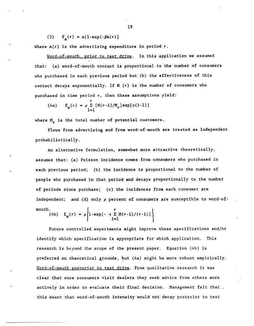
Word-of-mouth, prior to test drive. In this application we assumed
that: (a) word-of-mouth contact is proportional to the number of consumers
who purchased in each previous period but (b) the effectiveness of this
contact decays exponentially. If M (r) is the number of consumers who
purchased in time period r, then these assumptions yield:
(4a) fw(r) - p [M(r-i)/M.]exp[7(i-l)]i-1
where MI is the total number of potential customers.
Flows from advertising and from word-of-mouth are treated as independent
probabilistically.
An alternative formulation, somewhat more attractive theoretically,
assumes that: (a) Poisson incidence comes from consumers who purchased in
each previous period; (b) the incidence is proportional to the number of
people who purchased in that period and decays proportionally to the number
of periods since purchase; (c) the incidences from each consumer are
independent; and (d) only p percent of consumers are susceptible to word-of-
mouth. r(4b) fw () - p -exp[- 7 M(r-i)/(r-i)]
i-1
Future controlled experiments might improve these specifications and/or
identify which specification is appropriate for which application. This
research is beyond the scope of the present paper. Equation (4b) is
preferred on theoretical grounds, but (4a) might be more robust empirically.
Word-of-mouth posterior to test drive. From qualitative research it was
clear that once consumers visit dealers they seek advice from others more
actively in order to evaluate their final decision. Management felt that ,
this meant that word-of-mouth intensity would not decay posterior to test
20
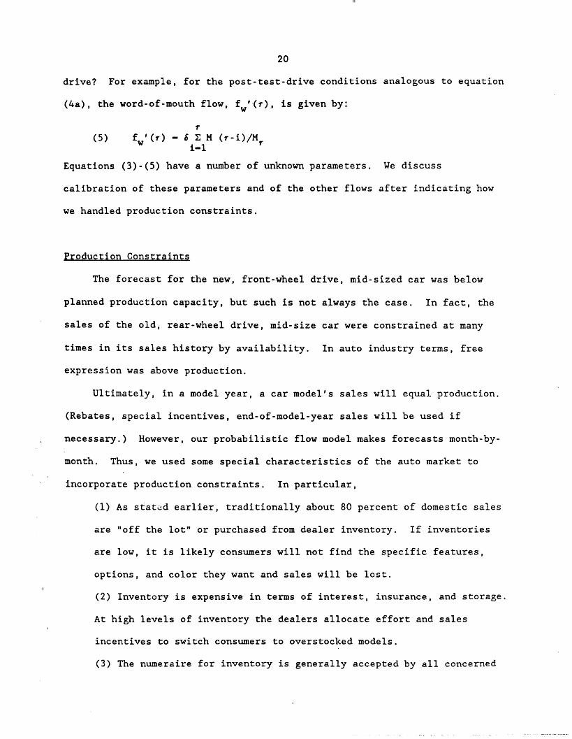
drive? For example, for the post-test-drive conditions analogous to equation
(4a), the word-of-mouth flow, fw'(r), is given by:
(5) fw'(t) - M (-i)/Mi-1
Equations (3)-(5) have a number of unknown parameters. We discuss
calibration of these parameters and of the other flows after indicating how
we handled production constraints.
Production Constraints
The forecast for the new, front-wheel drive, mid-sized car was below
planned production capacity, but such is not always the case. In fact, the
sales of the old, rear-wheel drive, mid-size car were constrained at many
times in its sales history by availability. In auto industry terms, free
expression was above production.
Ultimately, in a model year, a car model's sales will equal production.
(Rebates, special incentives, end-of-model-year sales will be used if
necessary.) However, our probabilistic flow model makes forecasts month-by-
month. Thus, we used some special characteristics of the auto market to
incorporate production constraints. In particular,
(1) As stated earlier, traditionally about 80 percent of domestic sales
are "off the lot" or purchased from dealer inventory. If inventories
are low, it is likely consumers will not find the specific features,
options, and color they want and sales will be lost.
(2) Inventory is expensive in terms of interest, insurance, and storage.
At high levels of inventory the dealers allocate effort and sales
incentives to switch consumers to overstocked models.
(3) The numeraire for inventory is generally accepted by all concerned
1I1

21
as "days supply," the number of units in stock divided by the current
sales rate. It is this stimulus to which dealers react.
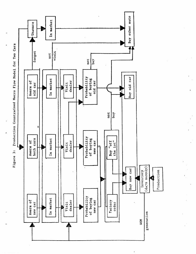
To incorporate these phenomena we expand the set of behavioral states to
include availability. See figure 3 for new and old car flows. In the
model, the awareness shown in the Figure 3 boxes is broken down as shown in
Figure 2, but for expositional simplicity this is not done in Figure 3. We
then model the availability probability, p(r), as:
(6) p(r) - l-exp(-AD(r)-e)
where D(r) is days supply at time period r: A and are parameters.
Days supply for the control car is observed from historical data and
calculated for the new car. Initial days supply for the test car is based on
management judgment and then calculated from the simulation results in later
periods. Management acceptance of the D(r) is critical. It must be
consistent with the macro-flow forecasts as well as consistent with their own
projected fine-tuning.
The number of people buying the car is now calculated as the fraction of
all potential purchasers who want to buy the car "off the lot" multiplied by
the availability (p(r)). Those who place a custom factory order and wait
(usually 8-12 weeks) are not reduced by the availability probability.
<Insert Figure 3, Production Constrained macro-flow...,' about here.>
Calibration and Fitting
The models shown in Figures 2 and 3 are a practical models. They
incorporate phenomena management feels are important in a way management can
accept. Yet, the models are complex -- we need many flow probabilities.
22
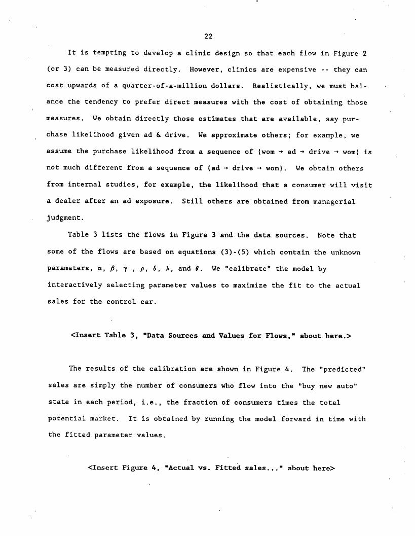
It is tempting to develop a clinic design so that each flow in Figure 2
(or 3) can be measured directly. However, clinics are expensive -- they can
cost upwards of a quarter-of-a-million dollars. Realistically, we must bal-
ance the tendency to prefer direct measures with the cost of obtaining those
measures. We obtain directly those estimates that are available, say pur-
chase likelihood given ad & drive. We approximate others; for example, we
assume the purchase likelihood from a sequence of (wom ad drive wom) is
not much different from a sequence of (ad - drive - wom). We obtain others
from internal studies, for example, the likelihood that a consumer will visit
a dealer after an ad exposure. Still others are obtained from managerial
judgment.
Table 3 lists the flows in Figure 3 and the data sources. Note that
some of the flows are based on equations (3)-(5) which contain the unknown
parameters, a, , , p, 6, A, and 0. We "calibrate" the model by
interactively selecting parameter values to maximize the fit to the actual
sales for the control car.
<Insert Table 3, Data Sources and Values for Flows,' about here.>
The results of the calibration are shown in Figure 4. The "predicted"
sales are simply the number of consumers who flow into the "buy new auto"
state in each period, i.e., the fraction of consumers times the total
potential market. It is obtained by running the model forward in time with
the fitted parameter values.
<Insert Figure 4, 'Actual vs. Fitted sales...' about here>
II
23
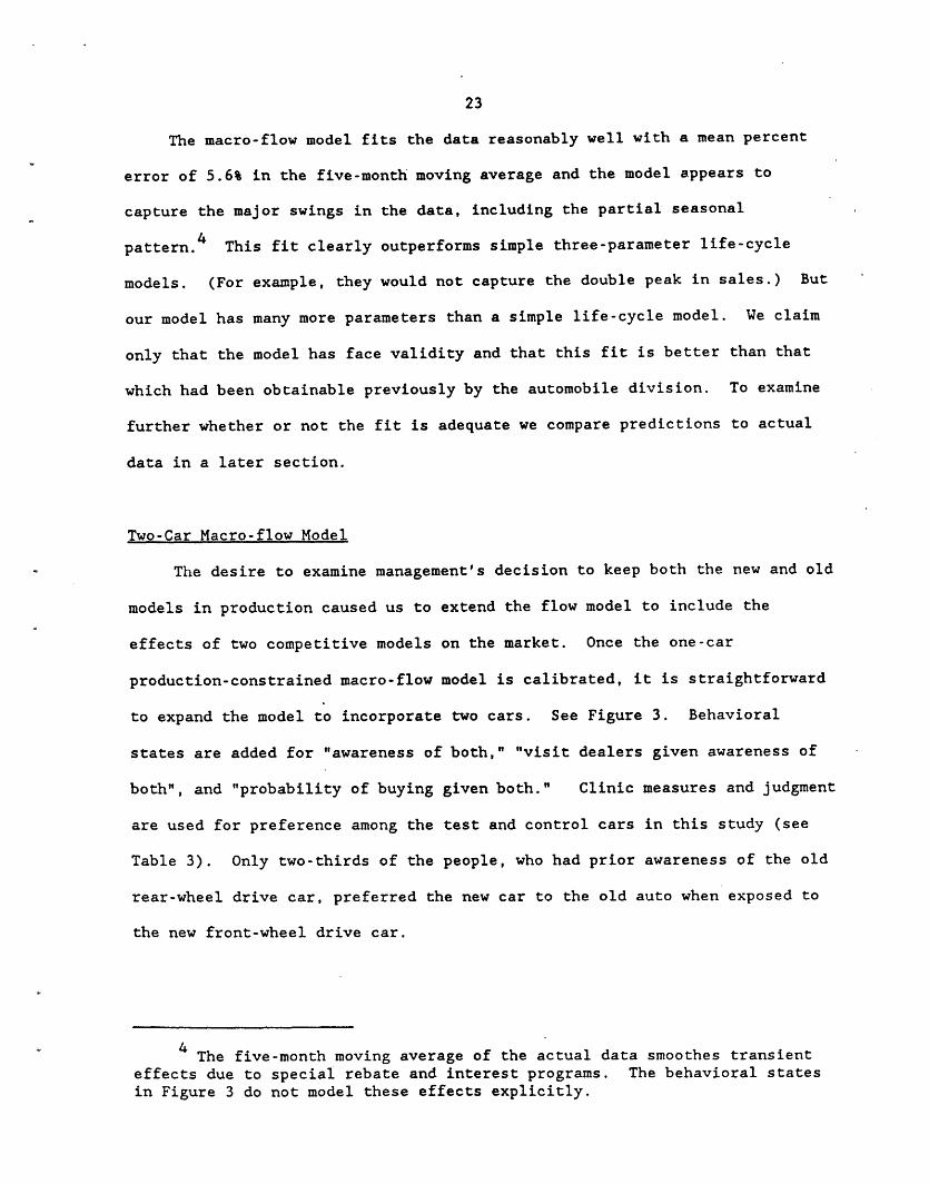
The macro-flow model fits the data reasonably well with a mean percent
error of 5.6% in the five-month moving average and the model appears to
capture the major swings in the data, including the partial seasonal
pattern.4 This fit clearly outperforms simple three-parameter life-cycle
models. (For example, they would not capture the double peak in sales.) But
our model has many more parameters than a simple life-cycle model. We claim
only that the model has face validity and that this fit is better than that
which had been obtainable previously by the automobile division. To examine
further whether or not the fit is adequate we compare predictions to actual
data in a later section.
Two-Car Macro-flow Model
The desire to examine management's decision to keep both the new and old
models in production caused us to extend the flow model to include the
effects of two competitive models on the market. Once the one-car
production-constrained macro-flow model is calibrated, it is straightforward
to expand the model to incorporate two cars. See Figure 3. Behavioral
states are added for "awareness of both," "visit dealers given awareness of
both", and "probability of buying given both." Clinic measures and judgment
are used for preference among the test and control cars in this study (see
Table 3). Only two-thirds of the people, who had prior awareness of the old
rear-wheel drive car, preferred the new car to the old auto when exposed to
the new front-wheel drive car.
The five-month moving average of the actual data smoothes transienteffects due to special rebate and interest programs. The behavioral statesin Figure 3 do not model these effects explicitly.

24
MANAGERIAL APPLICATION OF FLOW MODEL
Table 4 reports forecasts based on the macro-flow model. The base case
predictions are close to those in Table 2 -- still well below the production
target.
<Insert Table 4, Sales forecast and Strategy Simulations," about here>
The projected shortfall in sales put pressure on management to develop
strategies that would improve free expression sales. We simulated three
marketing strategies that were considered. The first strategy was a doubling
of advertising in an attempt to increase advertising awareness (the model was
run with advertising spending doubled). Table 4 indicates this would
increase sales somewhat, but not enough. Given its cost, this strategy was
rejected.
The next strategy considered was a crash effort to improve the
advertising copy to encourage more dealer visits. Assuming that such copy
would be attainable, we simulated forty percent more dealer visits. (The
model was run with dealer-visit flow-parameters multiplied by 1.4 for ad
aware conditions). The forecast was much better and actually achieved the
sales goals in year 2. Although a forty percent increase was viewed as too
ambitious, the simulation did highlight the leverage of improved copy that
encouraged dealer visits. A decision was made to devote resources toward
encouraging dealer visits. The advertising agency was directed to begin work
on such copy, especially for the identified segment of women currently
driving small cars.
III

25
The final decision evaluated was the effect of incentives designed to
increase the conversion of potential buyers who visit dealer showrooms. We
simulated a twenty percent increase in conversion (all dealer-visit flow
were parameters muliplied by 1.2). The leverage of this strategy was
reasonable but not as high as the improved advertising copy. This simulation
coupled with management's realization that an improvement would be difficult
to achieve on a national level (competitors could match any incentive
program) led management to a more conservative strategy which emphasized
dealer training.
The net result of the sales analysis was that management decided to make
an effort to improve dealer training and advertising copy, but that any
forecast should be conservative in its assumptions about achieving the 40
percent and 20 percent improvements.
The shortfall in projected sales, dealer pressure to retain the popular
rear-wheel drive car, and indications that production of the new car would be
delayed, led management to the decision (described earlier) to retain both
the old and the new cars. Initial thinking was that the total advertising
budget would remain the same but be allocated 25/75 between the old and new
cars. Evaluation of this strategic scenario required the two-car macro-flow
model.
The forecasts for the two-car strategy with the above advertising and
dealer's incentives tactics are shown in Table 5. The combined sales were
forecast to be higher than a one-car strategy in years 1 and 4, but lower in
years 2 and 3. Overall the delayed launch caused a net sales loss of roughly
48,000 units over 4 years. This is not dramatic, especially given potential
uncertainty in the forecast. However, the two car strategy did not achieve
the sales goal and made it more difficult to improve advertising copy and
26
dealer training. Once the production decision had been made and the
production delays were unavoidable, management was forced to retain the two-
car strategy. Our analysis suggested that it be phased out as soon as was
feasible.
<Insert Table 5, Sales Forecasts for Two-car Strategy," about here.>
This chain of events illustrates the value of a flexible, macro-flow
model. The world is not static. Often, unexpected events occur (dramatic
sales shortfalls, production delays) that were not anticipated when the
initial model was developed. In this case we could not evaluate the overall
two-car strategy with the Mod I analysis; management proceeded on judgment
and the information available. Once we developed the two-car macro-flow
model we could fine-tune the strategy to improve profitability and, in
retrospect, evaluate the basic strategy. More importantly, we now have the
tool (and much of the calibration) to evaluate multiple-car strategies for
other car lines.
PREDICTED VS. ACTUAL SALES
We turn now to a form of validation. Validation is always difficult
because management has the incentive to sell cars, not provide a controlled
laboratory for validation.
There are at least two components of deviations between actual and
predicted sales. If planned strategies are executed faithfully, the model is
likely to have some error and actual sales will not match predicted sales.
To evaluate this model, we are interested in this first component of error.
III
27
But as sales reports come in and unexpected events happen, management
modifies planned strategies to obtain greater profit. This, too causes
predicted sales to deviate from actual sales. For example, excess aggregate
inventories (across all car lines in the corporation) often encourages rebate
or interest rate incentives. Both of these increase and/or shift sales. We
are interested in these deviations to identify those actions which need to be
added in future model elaborations.
To examine both components of deviations we report two comparisons of
actual vs. predicted sales. In the first we compare predictions made prior
to launch with sales obtained during launch. In the second we input
managerial actions as they actually occurred and compare the adjusted
predictions to actual sales. When any adjustments are made we are
conservative and we include adjustments which hurt our accuracy as well as
help our accuracy. Together, the two comparisons give us an idea of which
deviations are due to model error and which deviations are due to changes in
managerial actions.
In our application, the advertising allocation changed, industry sales
were above the econometric forecast, special interest rate promotions were
employed, and production was delayed further for the new car. We report
first the unadjusted comparison and then a comparison adjusted for the
changes in advertising, industry sales, incentives, and production.
Table 6 reports the unadjusted predictions. Actual sales for the two
cars were well below the forecast. However, almost all of this deviation
occurs when we compare predicted sales for the new car to actual sales. The
forecasts for the existing car were close to actual. Recall the new car was
production constrained while the old car was not.

28
<Insert Table 6, 'Comparison of Actual Sales ... ," about here.>
We now attempt to decompose these deviations into deviations due to the
model and deviations due to management decisions. We do this by computing
the adjusted prediction.
The actual advertising allocation was 50/50 not 25/75 as planned. We
modify the direct inputs to the macro-flow model accordingly (see equation
3). Industry sales were above the economic forecasts. We modify the macro-
flow inputs accordingly. (Note that this modification works against
improving our fit.) There was a special interest rate incentive program for
the old car in months 11 and 12. We have no way to include this explicitly,
but will scrutinize months 11 and 12 carefully in the final comparison.
Production of the new car was delayed significantly. Production problems
reduced the availability of the popular V6 engines causing 80% of the old
cars in months 13 to 18 to be produced with the less popular V8 engines;
similar problems in months 13 to 18 caused a substitution of the less popular
standard transmissions in 33% of the new cars. We make these adjustments
with the production constrained model using the free expression preferences
among engines and transmissions from periods 1 to 12.
The adjusted forecasts are shown in Figure 5. The agreement is
acceptable -- the mean model error for the 18 months is now 8.8% (down from
46% in the unadjusted comparison). The agreement would have been much closer
had we been able to adjust for the incentive program on the old car in months
11 and 12. The overall cumulative predictive accuracy is good, but monthly
forecasts would have to be used with some caution.
<Insert Figure 5, "Comparison of Actual and Adjusted Forecasts," about here.>
I11
29
This application demonstrates the difficulty and complexity of
validation for durable goods forecasts. Production and marketing changes
from the original plan have a significant effect; adjustments must be made.
However, adjustments have the danger of being ad hoc and fulfilling the
researchers' desire for predictive accuracy. We have tried to guard against
these dangers with conservative adjustment and by reporting these adjustments
as fairly as possible. We recognize that full evaluation must await
independent applications of the model.
SUBSEQUENT APPLICATIONS
We have implemented the model in three other major car introductions.
The first was a new downsized "top of the line" luxury car that replaced its
larger predecessor. Clinic data indicated that the new car would be
preferred by a factor of 1.1 to the old car and the detailed dynamic forecast
indicated a 15 percent improvement in sales volume. But this was less
increase than had been desired. Because the clinic data indicated that the
old brand buyers liked the new car and were secure, the marketing was
oriented through increased advertising spending and copy towards import-
buyers who were identified as a high potential group in the clinic responses.
Copy also was based on building a perception of improved reliability which
was found in the market research to be a weak point (e.g., ads showed testing
the car in the outback of Australia). After those improvements, the car was
successfully launched and sales increased 25 percent above the old levels as
predicted by the model.
The next car studied was a full-size luxury two-door sedan that was
downsized in an attempt to double sales and meet the corporate fuel economy
30
standards. The clinic data indicated that the old buyers found the car to
be small and ordirnary, and they would have little interest in buying it. The
only group that liked it was import-buyers, but they did not like it as much
as other import options. The sales were forecast to be 50% of the old car's
level of sales. Advertising and promotion changes were of little help.
Unfortunately for the company, the forecast was correct and the first 12
months were 45% of the previous levels. This car should have been
repositioned but a subsequent change in the marketing management of the
company just after the final forecasts were made caused the bad news to be
ignored. The new division director wanted a success and did not want to
believe that the car could not be "turned around" before the launch.
The final car was a small two-door sports car that was subsequently
launched successfully. The clinic data showed that sufficient "free-
expression" demand existed to make an exclusive and efficient launch
possible in the first six months. That is, large advertising spending would
not be required and fully featured cars could be offered to those "lucky
enough to get one" because of limited production volumes. Private car
showings were arranged for target customers to position the launch as
exclusive. Higher prices could be supported in the first 9 months when
production capability was low, but management chose to keep a lower price
initially to avoid the perception of distress pricing and to maintain the
special tone of the introduction. Test drives were promoted because the
clinic showed significant increase in probability of purchase after people
experienced the comfortable and roomy, but sporty, ride and handling. After
six months, sales are within one standard deviation predictions.
The durable goods model proposed in this paper has also been implemented
on a PC home word-processing system and on a new camera. In all cases the
III

31
model, measures, and simulations were key components in management decisions
on how to target, position, communicate, and price the new product.
DISCUSSION
When we undertook the challenge to develop a prelaunch forecasting
system for new automobiles we hoped to develop a deeper understanding of the
managerial needs and the special challenges of durable goods forecasting. We
feel we have learned a lot in the seven years of applications.
Durable goods do present unique problems. The "price" forecasting
problem, validation of production constrained forecasting, search and
experience, and word-of-mouth (magazine reviews) are critical phenomena
relevant to durable goods. Addressing these issues has been challenging and
scientifically interesting. We hope that the applications described in this
paper enable the reader to appreciate better the needs of automobile (durable
goods) marketing managers. Clearly, many challenges remain. We summarize a
few here.
Applications Challenges
Perhaps the biggest challenge is efficient measurement. Clinics are
expensive -- sites must be leased, cars obtained, cars maintained, videos
produced, test drives set up, names obtained, consumers recruited, etc.
Macro models are data intensive. The advantage of making every flow explicit
leads one to recognize the need for detailed (and expensive) consumer
intelligence. In the applications described in this paper we made what we
believed to be efficient tradeoffs among data needs and data costs. The
industry would benefit from explicit cost/benefit analyses to optimize data
collection.
32
We can foresee the use of a computer with video disk interface as a
method to provide information more efficiently and effectively. Perhaps the
word-of-mouth spokesperson could be selected from a number of candidates
stored on the video disk. The spokesperson might be matched to demographic
and attitudinal characteristics of respondents to simulate the availability
to the respondents. The information would be respondent controlled and
responses recorded simulataneously as the information is processed and
perceptions and preferences change.
Another challenge is the cost of the vehicles. Hand-built prototypes
can cost $250,000 or more. Such prototypes are built as part of the
engineering development, but the operating division must obtain them for
clinic. Work is underway in the industry to determine whether fiberglass
mockups or other substitutes can be used to provide earlier forecasts of
consumer response. For example, at MIT, holograms are being used as full-
scale auto representations.
Scientific Challenges
Equations underlying the flow model (equations 3-5 and Figures 2 and 3)
represent the authors' experience but they are still somewhat ad hoc.
Research is needed on the best specifications of these flows. How many
levels should be created and how much segmentation by awareness should be
done?
In our applications to date we relied on "calibration" which mixed
direct measurement, modeling, judgment, and fitting. As we gain clinic
experience, one might consider constrained maximum-likelihood or Bayesian
estimation. For example, work is underway at Northwestern University to
adapt the continuous-time equations (Hauser and Wisniewski 1982a) to maximum
likelihood estimation via super computers.
III

33
Extensions
A number of extensions are possible to our auto prelaunch forecasting
model. For example, the two-car model could be extended to a full product-
line formulation. A number of new phenomena could be added: dealer
advertising, dealer visits without prior awareness, multiattribute effects on
preference, risk, and consumer budgeting. These modifications are feasible,
but they add to the complexity and increase measurement/analysis costs. In
each case these extensions should be evaluated on a cost and benefit basis
before embarking on a more complex model.
Perhaps the most important extension is the use of marketing science
analyses for pre-investment as well as prelaunch decisions. Early modeling
of the "voice of the customer" should prove valuable in integrating
marketing, engineering, and production to develop automobiles that satisfy
long term consumer needs.
The auto industry is now experimenting with test/control clinic
methodologies to understand the causal links between engineering design
features and attributes that consumers desire. Perhaps future macro-flow
analyses can link design improvements, such as anti-lock brakes, to sales.
Although much research is suggested by our efforts, the initial results
suggest customer-flow models are useful in capturing the unique aspects of
durable goods marketing. The models can be calibrated empirically and
implemented with managers.
R1
REFERENCES
1. Bass, Frank M. (1969), "A New Product Growth Model for ConsumerDurables," Management Science, 15, 5 (January), pp. 215-227.
2. Goettler, Peter N. (1986), "A Pre-market Forecasting Model for NewConsumer Durables: Development and Application," Master's Thesis, SloanSchool of Management, M.I.T., Cambridge, MA 02139.
3. Hauser, John R. and Don Clausing (1988), "The House of Quality," HarvardBusiness Review, 66, 3, (May-June), pp. 63-73.
4. and Glen L. Urban (1986), "The Value Priority Hypotheses forConsumer Budget Plans," Journal of Consumer Research, 12, (March), pp.446-462.
5. and Kenneth J. Wisniewski (1982a), "Dynamic Analysis ofConsumer Response to Marketing Strategies," Management Science, 28, 5,(May), pp. 455-486.
6. and Kenneth J. Wisniewski (1982b), "Application, PredictiveTest, and Strategy Implications for a Dynamic Model of ConsumerResponse," Marketing Science 1, 2, (Spring), pp. 143-179
7. Heeler, R.M. and T.P. Hustad (1980), "Problems in Predicting New ProductGrowth for Consumer Durables," Management Science, 26, 10, (October), pp.1007-1020.
8. Horsky, Dan and Leonard S. Simon (1983), "Advertising and tle Diffusionof New Products," Marketing Science, 2, 1, (Winter), pp. 1-17.
9. Jeuland, Abel P. (1981), "Parsimonious Models of Diffusion of Innovation.Part A: Derivations and Comparisons, Part B: Incorporating the Variableof Price," mimeo, University of Chicago, IL, June.
10. Juster, Frank T. (1966), "Consumer Buying Intentions and PurchaseProbability: An Experiment in Survey Design," Journal of the AmericanStatistical Association, 61, pp. 658-96.
11. Kalish, Shlomo (1985), "New Product Adoption Model with Price,Advertising, and Uncertainty," Management Science, 31, 12, (December),pp. 1569-1585.
12. Little, John D.C. (1970), "Models and Managers: The Concept of a DecisionCalculus," Management Science, 16, 8, (April), pp. 466-485.
13. (1975), "BRANDAID: A Marketing Mix Model: Structure,Implementation, Calibration, and Case Study," Operations Research, 23, 4,(July-August), pp. 628-673.
14. _ (1979), "Decision Support Systems for Marketing Managers,"Journal of Marketing, 43, (Summer), pp. 9-26.
Ill

R2
15. Mahajan, Vijay and Eitan Muller (1979), "Innovation, Diffusion, and NewProduct Growth Models in Marketing," Journal of Marketing, 43, 4, (Fall),pp. 55-68.
16. , and Roger A. Kerin (1984),"Introduction Strategy for New Products with Positive and Negative Wordof Mouth," Management Science, 30, 12, (December), pp. 1389-1404.
17. Mitchell, Russell (1986), "How Ford Hit the Bull's-eye with Taurus,"Business Week, (June 30), pp. 69-70.
18. Pringle, Lewis G., R. Dale Wilson, and Edward I. Brody (1982), "NEWS: ADecision Oriented Model for New Product Analysis and Forecasting,"Management Science, vol. 1, No. 1, (Winter 182), pp. 1-30.
19. Roberts, John H. and Glen L. Urban (1987), "New Consumer Durable BrandChoice: Modeling Multiattribute Utility, Risk and Belief Dynamics,"Management Science, Vol. 34, No. 2 (February), pp. 167-85.
20. Robinson, Bruce and Chet Lakhani (1975), "Dynamic Price Models for NewProduct Planning," Management Science, 21, (June), pp. 1113-1132.
21. Silk, Alvin J. and Glen L. Urban (1978), "Pre-Test Market Evaluation ofNew Packaged Goods: A Model and Measurement Methodology," Journal ofMarketing Research, 15, (May), pp. 171-191.
22. Silverman, Lisa (1982), "An Application of New Product Growth Modeling toAutomobile Introductions," Master's Thesis, Sloan School of Management,M.I.T., Cambridge, MA 02139, June.
23. Srinivasan, K.V. (1988), "Effect of Consumer Categorization Behavior onNew Product Sales Forecasting," Master's Thesis, Sloan School ofManagement, M.I.T., Cambridge, MA 02139, June.
24. Urban, Glen L. (1968), "A New Product Analysis and Decision Model,"Management Science, Vol. 14, No. 8 (April), pp. 490-517.
25. (1970), "SPRINTER Mod III: A Model for the Analysis ofNew Frequently Purchased Consumer Products," Operations Research, 18, 5,(September-Octobter), pp. 805-853.
26. and John R. Hauser (1980), Design and Marketing of NewProducts, Englewood Cliffs, NJ: Prentice-Hall.
27. Wind, Yoran and Vijay Mahajan (1986), Innovation Diffusicn Models of NewProduct Acceptance, Ballinger Publishing Co., Cambridge, MA.

Table 1: Relative Preference Conditioned by Information Sequence
New car Control car Difference Ratio
Information Sequence (n=sample size) (n=sample size) (new-control) (new/control)
1. concept awareness 13.3 (336) 14.2 (167) -0.9 .94
2. concept then wom(+) 14.7 (85) 16.6 (82) -1.9 .88
3. concept then wom(-) 10.3 (86) 16.6 (46) -5.3* .62
4. concept then drive 18.5 (165) 21.2 (82) -2.7 .87
5. conceptwom(+)-drive 16.4 (85) 21.0 (37) -4.6* .78
6. concept-wom(-)-drive 14.0 (86) 23.1 (46) -9.1* .61
7. concept-drive-wom(+) 16.7 (91) 18.5 (41) -1.8 .90
8. concept-drive-wom(-) 16.6 (74) 18.2 (46) -1.6 .91
Significant at 10% based on comparison of means across subsamples
ASee Figure 1 for experimental flow diagram for sequence codes.
I

Table 2
Top-Line Forecasts for
Year of Life Cycle
1
2
3
4
Sales
274,000
376,000
247,000
191,000
Share
9.8
11.0
8.5
7.4
New Mid-Size Car
Difference from Target
176,000
124,000
203,000
259,000

TABLE 3
NEW INPUTS AND SOURCES FOR TWO CAR MODEL*
Source
Target Group Size Set in plan for number of buyers
Category Sales (monthly) G.M. econometric forecasts
Awareness
- advertising spending (monthly)
- a, , forgetting (flow fromaware of ad, WOM, or both tounaware) (see equation 3)
- aware of both cars
planned levels
fit to past awareness, spendingand sales for control car andmodify judgmentally for changesfor new car
awareness proportion for newcar times awareness proportionfor old car
In Market
- fraction of those awarewho are in market
calculate as category salesdivided by target group size forall awareness conditions
Visit Dealer
- fraction who visit dealergiven ad aware
- fraction who visit dealergiven ad and WOM aware
- fraction who visit dealer givenWOM aware
- probability of visit dealer ifaware of both cars
clinic measured probabilityof purchase after ad exposure(see Figure 1)
clinic measured probability ofpurchase after WOM video tapeexposure
judgmentally set given abovetwo values
probabiity of visit for new carin clinic after awareness among thoserespondents who were aware of the oldcar before the clinic
Purchase
- probability of buying new cargiven awareness condition:
(l)ad aware before visit and noother awareness
clinic measure probability ofpurchase after ad exposure andtest drive
Inputs

TABLE 3 (continued)
(2) ad aware before visit and WOM
(3) ad and WOM aware before visit
(4) ad aware before and after visit
(5) WOM aware before and no otherawareness
(6) WOM before and after visit
probability of buying new carif aware of new car andold car
clinic measure probability ofpurchase after ad, test drive andWOM exposure
clinic probability of purchase afterad, WOM and test drive
judgmentally set based on (1),(2),(3)
judgmentally set based on (1),(2),(3)
judgmentally set based on (1),(2),(3)
probability of buying new car in clinicamong those respondents who were awareof the old car before the clinic
Word of Mouth Communication
- p, (equation 4a)
- 6 (equation 5)
- aware of ads and WOM
managerial judgment and fit to pastdata on fraction of awareness due toword of mouth and control car sales
past survey data, judgment, and fitto control car sales
probability of ad aware timesprobability of WOM aware
Production
- levels of production (monthly)
- A, 8 (equation 6)
- fraction of buyers who wantto buy "off the lot"
planned levels
managerial judgment, fit to past dataon control car sales, and pastresearch studies
past studies and judgment
*Analogous procedures are used for control car based on control cell measuresin the clinic and past data.

III
TABLE 4SALES FORECASTS AND STRATEGY SIMULATIONS (in Units)
Base Case
281,000334,000282,000195,000
Advertising AdvertisingSpending CopyDoubled Improved 40%
334,000370,000330,000225,000
395,000477,000405,000273,000
DealerIncentivesImproved 20%
340,000406,000345,000234,000
Year
1234

TABLE 5SALES FORECASTS FOR TWO-CAR STRATEGY (in Units)
New Model
181,000213,000174,000121,000
Old Model
103,00089,00080,00084,000
Combined Sales
284,000301,000254,000205,000
Year
1234

TABLE 6COMPARISON OF ACTUAL SALES TO UNADJUSTED PREDICTIONS
1st .6 months
2nd6 months
3rd6 months TOTAL
ACTUALUNADJUSTED PREDICTIONPERCENT DIFFERENCE
97,000 119,000133,000 151,000
37% 27%
90,000162,000
80%
306,000446,000
46%

Figure 1
Experimental Desipn of Sequential InforimationExposure in Clinic t(x) = Sequence Codesi
ExistingCar Data
ConsiderationChoice
Concept AdExposure
(1)r~~~~~~~~
+ Video(2)
I
Drive(4)
L . _L
- Video(3) Ilwr
Drive(5,6)
_ -,
+ Video(7)
- Video(8)
I _ -
I
I...- .
I .
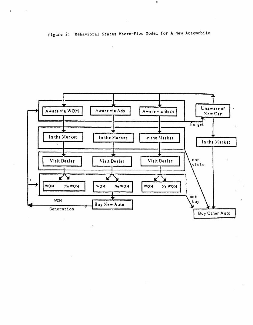
Figure 2: Behavioral States Macro-Flow Model for A New Automobile
(
03
H
owU4,-40)0
o
L:
00
u-ocd,4
cu
4ri
4ui0V:
0
Li
C:0,to
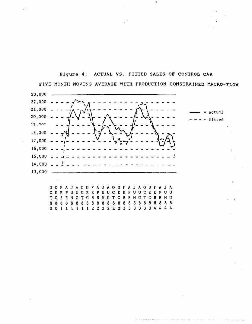
Figure 4: ACTUAL VS. FITTED SALES OF CONTROL CAR
FIVE MONTH MOVING AVERAGE WITH PRODUCTION CONSTRAINED MACRO-FLOW
23,000
·1 Fn --LZ, VVV - -
2 1,000 - -
20,000 - -
1 9 , '. _
18,000 - -
17,000- -
t I ---
- = actual
-- - = fitted
itU Q_- - ------------ -- - -
15,000 _ - - -
14,000 -
13,000
ODFAJAODFAJAODFAJAODF A J AC E E P U U C E E P U U C E E P UUC E E P U UT C B R N G T C B RN G T C B RN G T C 8 R N G88888888888888888888888800 1 1 1 1 1 1 22 22 2 23 3 33 3 3 4 4 4 4
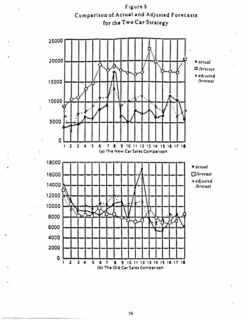
Figure 5
Comparison of Actual and Adjusted Forecasts
for the Two Car Strategy
1 2 3 4 5 6 7 8 9 10 11 12 14 IS 16 17 1(a) the New Car Sles Comparison
36
2500C
2000(
15000
10000
5000
.o
* actual
3O orecast
X adljIstedorecss t
18000
16000
14000
12000
10000
8000'
6000
4000
2000
0
* actual
Dfortcatx adjusted
forecat
1 2 3 4 5 6 7 8 9 10 11 12 13 14 IS is 17 18(b) The Old Car Sales Comparison