PRELIMINARY DEVELOPMENT OF A BIO-INSPIRED

HEXAPOD CLIMBING ROBOT RELYING ON DRY ADHESIVES

by

Yasong Li B. Eng., South China Agricultural University, 2006

THESIS SUBMITTED IN PARTIAL FULFILLMENT OF THE REQUIREMENTS FOR THE DEGREE OF

MASTER OF APPLIED SCIENCE

In the School of Engineering Science

© Yasong Li 2009

SIMON FRASER UNIVERSITY

Summer 2009

All rights reserved. However, in accordance with the Copyright Act of Canada, this work may be reproduced, without authorization, under the conditions for Fair Dealing. Therefore, limited reproduction of this work for the purposes of private

study, research, criticism, review and news reporting is likely to be in accordance with the law, particularly if cited appropriately.

Last revision: Spring 09

Declaration of Partial Copyright Licence The author, whose copyright is declared on the title page of this work, has granted to Simon Fraser University the right to lend this thesis, project or extended essay to users of the Simon Fraser University Library, and to make partial or single copies only for such users or in response to a request from the library of any other university, or other educational institution, on its own behalf or for one of its users.

The author has further granted permission to Simon Fraser University to keep or make a digital copy for use in its circulating collection (currently available to the public at the “Institutional Repository” link of the SFU Library website <www.lib.sfu.ca> at: <http://ir.lib.sfu.ca/handle/1892/112>) and, without changing the content, to translate the thesis/project or extended essays, if technically possible, to any medium or format for the purpose of preservation of the digital work.

The author has further agreed that permission for multiple copying of this work for scholarly purposes may be granted by either the author or the Dean of Graduate Studies.

It is understood that copying or publication of this work for financial gain shall not be allowed without the author’s written permission.

Permission for public performance, or limited permission for private scholarly use, of any multimedia materials forming part of this work, may have been granted by the author. This information may be found on the separately catalogued multimedia material and in the signed Partial Copyright Licence.

While licensing SFU to permit the above uses, the author retains copyright in the thesis, project or extended essays, including the right to change the work for subsequent purposes, including editing and publishing the work in whole or in part, and licensing other parties, as the author may desire.

The original Partial Copyright Licence attesting to these terms, and signed by this author, may be found in the original bound copy of this work, retained in the Simon Fraser University Archive.

Simon Fraser University Library Burnaby, BC, Canada

ABSTRACT

Biologists have recently discovered that dry adhesion on the feet of

geckos and hunting spiders provides remarkable adhesive forces generated by

van der Waals forces. Different researches have attempted to mimic the

adhesive used by geckos and spiders adhesives through novel manufacturing

processes. This thesis presents the preliminary analysis and development of

hexapod climbing robot prototypes designed to take advantage of the special

features that dry adhesion offers. A kinematic analysis was performed, which

was validated through an experimental procedure. The two robotic prototypes,

which were developed following engineering design procedures, are presented

and discussed in this thesis. Preliminary investigations on optimal trajectory and

joint torques for enhancing dry adhesive properties are introduced for a future in

depth analysis and use in climbing platforms.

Keywords: climbing robot; kinematics; hexapod; dry adhesion; bio-inspired

iii

DEDICATION

I dedicate this thesis to my family.

To mom and dad, for your unconditional love and support.

To grandma, the first teacher in my early days.

To grandpa, the respectable man forever.

iv

ACKNOWLEDGEMENTS

I would like to dedicate faithful thanks to my senior supervisor, Dr. Carlo

Menon, who provided such a great topic and helped me through the research,

and also for teaching me how to become a professional.

I also extend my acknowledgements to Dr. Ash Parameswaran and Dr.

Shahram Payandeh, for the inspiring lessons and advice you gave; Dr. Daniel

Sameoto, you are always my good example; Gary Houghton, for your help in

rapid prototyping machine; Gary Shum and Marius Haiducu, for helping in huge

amount of ordering forms; and all the faculty members, staffs and technicians

who run the school in good condition.

Here I also would like to thank my colleagues and friends (alphabetically):

Ausama Ahmed, Bastian Tietjen, Chris Martens, Claire Wu, Dr. Cormac

Sheridan, Dariush Sahebjavaher, David Tang, Doris Liu, Isacco Pretto, Jenny

Ma, Jyh-Yuan Yeh, Kaveh Kianfar, Menita Prasad, Nathan Cheng, Nathaniel

Seung, Nina Sauthoff, Simon Ruffieux, Ted Meredith, Wen Shi, Xiaochuan Sun,

Xingjie Jiang, and Zeeshan Khokhar. You all make Vancouver and SFU such a

nice place to stay.

Last, thank GOD there is such a discipline I enjoy with passion!

v

TABLE OF CONTENTS

Approval .............................................................................................................. ii Abstract .............................................................................................................. iii Dedication .......................................................................................................... iv Acknowledgements ............................................................................................ v Table of Contents .............................................................................................. vi List of Figures .................................................................................................. viii List of Tables ...................................................................................................... x Chapter 1  Introduction ................................................................................... 1 

1.1  Motivation ........................................................................................... 2 1.2  Objective .......................................................................................... 13 1.3  Thesis outline ................................................................................... 14 1.4  Thesis contributions ......................................................................... 15 

Chapter 2  Robot Design configurations and kinematic analysis ............. 17 2.1  Design configurations ....................................................................... 17 2.2  Introduction to kinematic analysis ..................................................... 19 2.3  First scenario: serial manipulator analysis ........................................ 19 

2.3.1  Direct kinematics ........................................................................... 20 2.3.2  Inverse kinematics ........................................................................ 24 2.3.3  Singularity ..................................................................................... 28 

2.4  Second scenario: parallel platform analysis ..................................... 31 2.5  Introduction to the local ground coordinate ...................................... 37 2.6  Chapter conclusion ........................................................................... 39 

Chapter 3  Mechanical and mechatronic design ........................................ 40 3.1  Manufacturing of robot construction part .......................................... 40 3.2  Prototype 1: hexapod using servo motor electronics ........................ 41 

3.2.1  Mechatronic system analysis ........................................................ 41 3.2.2  Mechanical structure of modified servo joint ................................. 44 3.2.3  Electronics features and adaption to the robot .............................. 47 3.2.4  Robot performance ....................................................................... 49 

3.3  Prototype 2: hexapod with motor driven joints .................................. 50 3.3.1  Mechatronic system analysis ........................................................ 51 3.3.2  Motor control signal ....................................................................... 53 3.3.3  Sensor selection and tests ............................................................ 54 3.3.4  Controller design and other electronics ......................................... 59 

vi

3.4  Discussion and conclusion ............................................................... 61 Chapter 4  Kinematic validation and development of control

strategies ..................................................................................... 63 4.1  Serial manipulator kinematics........................................................... 63 

4.1.1  MATLAB simulation ...................................................................... 63 4.1.2  Position control test based on Prototype 2 .................................... 67 

4.2  Parallel manipulator kinematics ........................................................ 70 4.2.1  Data generated in MATLAB .......................................................... 70 4.2.2  Simulation with WebotsTM ............................................................. 72 

4.3  Robot test in full step sequence ....................................................... 73 4.3.2  Robot climbing on a vertical wall ................................................... 76 

4.4  Trajectory selection for releasing the dry adhesive .......................... 79 4.4.1  Theory of peeling an elastic thin film ............................................. 79 4.4.2  Power consumption test for various peeling angles ...................... 80 

4.5  Optimizing the adhesive force .......................................................... 84 4.5.1  Optimal leg angle for maximizing the adhesive force .................... 84 4.5.2  Auto-preloading with optimized leg angle ..................................... 86 

4.6  Experimental validation of optimal joint torques for stable adhesion ........................................................................................... 88 

4.6.1  Experimental setup ....................................................................... 89 4.6.2  Test procedure and results ........................................................... 91 

4.7  Discussion and conclusion ............................................................... 94 Chapter 5  Towards a future design – tether actuated joint ...................... 96 Chapter 6  Conclusions and future work................................................... 101 

6.1  Conclusions .................................................................................... 101 6.2  Future work .................................................................................... 103 

6.2.1  Four joints in each leg ................................................................. 103 6.2.2  Joints with tether actuation ......................................................... 104 

Appendices ..................................................................................................... 105 Appendix A: Force distribution during walking ............................................... 105 Appendix B: Specification of servo motor HS-311 ......................................... 109 Appendix C: Specification of mini-motor GH6124S ....................................... 110 Appendix D: Specification of mini-motor GM15 ............................................. 113 Appendix E: Relationship between output voltage and rotary position of

HMC1512 ....................................................................................... 114 Appendix F: Calibration of Maxon RE25 motor ............................................. 115 

Bibliography .................................................................................................... 117 

vii

LIST OF FIGURES

Figure 1-1: Multi-scale adhesion mechanism in the spider Cupiennius salei. ...................................................................................................... 3 

Figure 1-2: Wheel climbing robots. ....................................................................... 6 Figure 1-3: Gecko-inspired robots. ....................................................................... 8 Figure 1-4: Spine embedded climbing robots. .................................................... 10 Figure 2-1: Anthropomorphic arm and its workspace. ........................................ 19 Figure 2-2: Coordinate assignment in configuration 1. ....................................... 20 Figure 2-3: Coordinates assignment in configuration 2. ..................................... 22 Figure 2-4: 2D graph for geometry analysis of configuration 2. .......................... 25 Figure 2-5: Two situations for the end effector reaching same position .............. 26 Figure 2-6: 2D graph for geometry analysis of configuration 1. .......................... 28 Figure 2-7: Robot model shown in parallel platform. .......................................... 32 Figure 2-8: Geometry representation of parallel robot situation .......................... 35 Figure 2-9: Local ground coordinate example .................................................... 39 Figure 3-1: Design of Prototype 1 ....................................................................... 42 Figure 3-2: Original structure of HS-311 Servo motor. ....................................... 43 Figure 3-3: Data flow of Prototype 1. .................................................................. 44 Figure 3-4: Assembly of one joint in Prototype 1 ................................................ 46 Figure 3-5: (a) SSC-32, batteries for servo controller and servo motors,

and the Bluetooth modem. (b) User interface of Visual Sequencer. .......................................................................................... 48 

Figure 3-6: Second prototype with electronics, connectors and feet .................. 51 Figure 3-7: Construction of one joint in Prototype 2 ............................................ 53 Figure 3-8: Potentiometer test result. ................................................................. 55 Figure 3-9: Application process of magneto-sensitive sensor ............................ 57 Figure 3-10: Magneto-sensitive sensor test result.. ............................................ 58 Figure 3-11: Block diagram of controller design in LabVIEW 8.2........................ 60 Figure 3-12: Control loop in one joint of Prototype 2. ......................................... 61 Figure 4-1: Single leg kinematic validation. ........................................................ 66 

viii

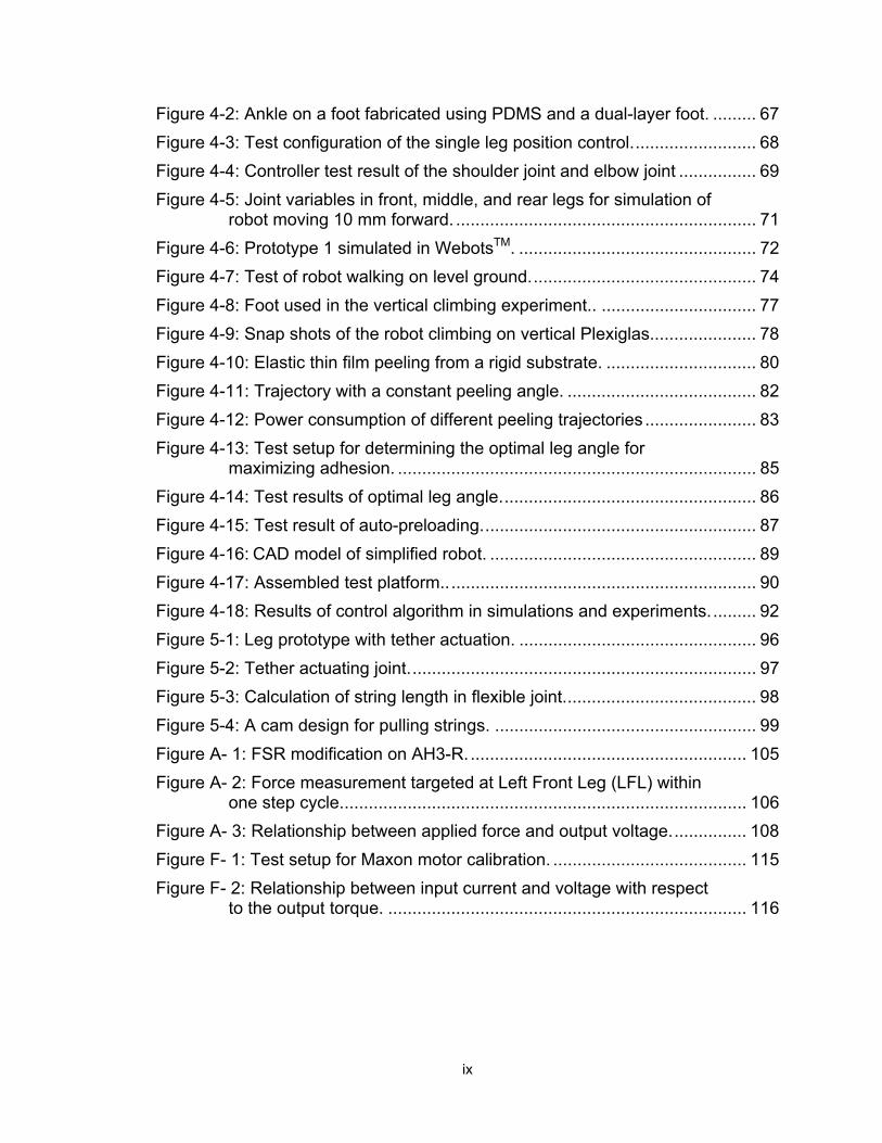
Figure 4-2: Ankle on a foot fabricated using PDMS and a dual-layer foot. ......... 67 Figure 4-3: Test configuration of the single leg position control. ......................... 68 Figure 4-4: Controller test result of the shoulder joint and elbow joint ................ 69 Figure 4-5: Joint variables in front, middle, and rear legs for simulation of

robot moving 10 mm forward. .............................................................. 71 Figure 4-6: Prototype 1 simulated in WebotsTM. ................................................. 72 Figure 4-7: Test of robot walking on level ground. .............................................. 74 Figure 4-8: Foot used in the vertical climbing experiment.. ................................ 77 Figure 4-9: Snap shots of the robot climbing on vertical Plexiglas.. .................... 78 Figure 4-10: Elastic thin film peeling from a rigid substrate. ............................... 80 Figure 4-11: Trajectory with a constant peeling angle. ....................................... 82 Figure 4-12: Power consumption of different peeling trajectories ....................... 83 Figure 4-13: Test setup for determining the optimal leg angle for

maximizing adhesion. .......................................................................... 85 Figure 4-14: Test results of optimal leg angle. .................................................... 86 Figure 4-15: Test result of auto-preloading. ........................................................ 87 Figure 4-16: CAD model of simplified robot. ....................................................... 89 Figure 4-17: Assembled test platform.. ............................................................... 90 Figure 4-18: Results of control algorithm in simulations and experiments. ......... 92 Figure 5-1: Leg prototype with tether actuation. ................................................. 96 Figure 5-2: Tether actuating joint. ....................................................................... 97 Figure 5-3: Calculation of string length in flexible joint. ....................................... 98 Figure 5-4: A cam design for pulling strings. ...................................................... 99 Figure A- 1: FSR modification on AH3-R. ......................................................... 105 Figure A- 2: Force measurement targeted at Left Front Leg (LFL) within

one step cycle. ................................................................................... 106 Figure A- 3: Relationship between applied force and output voltage. ............... 108 Figure F- 1: Test setup for Maxon motor calibration. ........................................ 115 Figure F- 2: Relationship between input current and voltage with respect

to the output torque. .......................................................................... 116 

ix

x

LIST OF TABLES

Table 1-1: Comparison among exsiting climbing robot utilized micro/nano adhesion structures ............................................................................. 12 

Table 2-1: DH parameters in serial manipulator for configuration 1. ................... 23 Table 2-2: DH parameters in serial manipulator for configuration 2. ................... 21 Table 3-1: Comparison of Prototype 1 and 2. ..................................................... 62 Table 4-1: Joint torques for model fitting ............................................................ 91 Table 4-2: Test result with Minimax control logic. ............................................... 93 Table B- 1: Specification of servo motor HS-311. ............................................. 109 Table C- 1: Mechanical details and specification of GH612 series 6mm

mini-motors ........................................................................................ 111 Table C- 2: Performance of GH612 series mini-motors at constant voltage

of 3 V. ................................................................................................ 112 Table D- 1: Specification of GM15 mini-motor. ................................................. 113 

CHAPTER 1 INTRODUCTION

Interest in studying climbing robots has grown rapidly in the recent

decade. Research can be categorized in four key areas of application: (1)

servicing (e.g., maintenance of skyscrapers, ships' hulls, nuclear plants, etc.); (2)

rescue (e.g., during fire, earthquakes, landslides, etc.); (3) security (e.g.,

surveillance, inspection, and military operations in buildings, extreme natural

environments, etc.); and (4) space (e.g., planetary exploration, Intra-Vehicular

Activities, Extra-Vehicular Activities, etc.) [1].

Among natural climbers, some creatures, such as geckos and spiders

stand out, as they can climb on almost all kinds of surfaces, even upside down.

Biologists have determined that their spectacular climbing ability is mainly due to

the nano-/micro-scale structures on their feet. These structures have been

named “dry adhesives”, as their adhesion relies on van der Waals forces rather

than tacky materials [2]. Biological dry adhesives are lightweight, self-cleaning

and have a high safety factor.1 The manufacture of synthetic dry adhesives has

been proven to be possible [3-7], and it is potentially suitable to enable the

development of climbing robots for different applications [8-15].

This thesis focuses on the design of a potentially robust and energy

efficient climbing mechanism utilizing dry adhesion. The proof-of-concept

prototypes were developed to show the ability of vertical climbing.

1 Safety factor is the relationship between body weight and the maximum adhesive force.

1

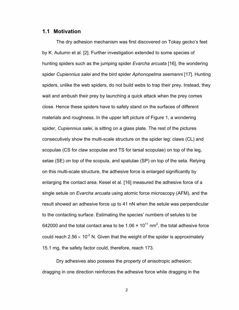
1.1 Motivation

The dry adhesion mechanism was first discovered on Tokay gecko’s feet

by K. Autumn et al. [2]. Further investigation extended to some species of

hunting spiders such as the jumping spider Evarcha arcuata [16], the wondering

spider Cupiennius salei and the bird spider Aphonopelma seemanni [17]. Hunting

spiders, unlike the web spiders, do not build webs to trap their prey. Instead, they

wait and ambush their prey by launching a quick attack when the prey comes

close. Hence these spiders have to safely stand on the surfaces of different

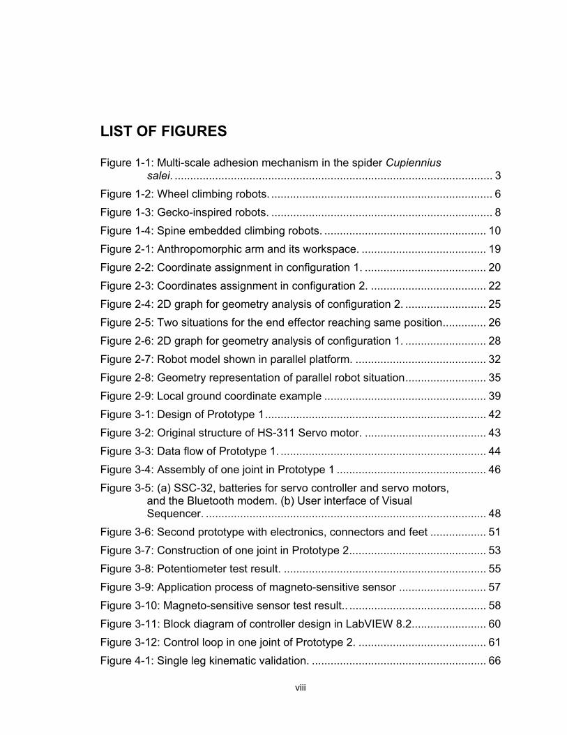
materials and roughness. In the upper left picture of Figure 1, a wondering

spider, Cupiennius salei, is sitting on a glass plate. The rest of the pictures

consecutively show the multi-scale structure on the spider leg: claws (CL) and

scopulae (CS for claw scopulae and TS for tarsal scopulae) on top of the leg,

setae (SE) on top of the scopula, and spatulae (SP) on top of the seta. Relying

on this multi-scale structure, the adhesive force is enlarged significantly by

enlarging the contact area. Kesel et al. [16] measured the adhesive force of a

single setule on Evarcha arcuata using atomic force microscopy (AFM), and the

result showed an adhesive force up to 41 nN when the setule was perpendicular

to the contacting surface. Estimating the species’ numbers of setules to be

642000 and the total contact area to be 1.06 × 1011 nm2, the total adhesive force

could reach 2.56 × 10-2 N. Given that the weight of the spider is approximately

15.1 mg, the safety factor could, therefore, reach 173.

Dry adhesives also possess the property of anisotropic adhesion;

dragging in one direction reinforces the adhesive force while dragging in the

2

opposite direction releases the adhesive force. Autumn et al. [18] proposed the

term programmable adhesive to describe the gecko’s ability to preload and drag

at angels smaller than 30 degrees to turn on the adhesive and increasing the

angle to easily turn off the adhesive. In the case of spiders, Niederegger et al.

[17] proposed that spiders push the tarsal to reinforce the adhesion and pull to

release the adhesion, due to the nano-hair arrangement on the spider legs.

Figure 1-1: Multi-scale adhesion mechanism in the spider Cupiennius salei. A) Spider resting on a tilted glass plate, B) Claws and scopula, C) Tip of single seta, D) Microtrichia with spatula at their tips. (Picture cited from Niederegger and Gorb, 2006. [17])

3

Several attempts have been made to replicate natural dry adhesion since

confirming the dry adhesion on gecko’s feet. The first attempts of manufacturing

synthetic dry adhesion were reported by Campolo et al. [19], Sitti and Fearing

[20], and Geim et al. [21] in 2003. These early attempts focused on replicating

the nano-structures, but the fibers (diameter of several hundred nanometers)

tended to be clump together, therefore, the samples were not sticky as expected.

Afterwards, fabrication of synthetic dry adhesion started to focus on a bigger

scale of fibers (with diameters varying from several microns to several hundred

microns) [22-24]. Those adhesive designs tried to replicate the anisotropic

property of natural dry adhesion by manufacturing fibers at a certain angle to the

substrate or by adding asymmetric structures on the fibers. Performance was

enhanced and, therefore, enabled a few successful climbing robots to employ

these adhesive designs.

Following this enhancement, dry adhesive development grew rapidly,

allowing climbing robots to use different shapes and functions of dry adhesives.

During early exploration of developing climbing robot utilizing dry adhesion, three

key criteria were identified in [13] for reliable climbing robot using dry adhesion:

(1) maximize the attachment area, (2) apply a preload between the vehicle and

the surface to increase the attachment force, (3) use a peeling mode to detach

the dry adhesion. Using these criteria, the design of a climbing robot should

maximize the adhesion efficiency by adapting unique characteristics of the dry

adhesives.

4

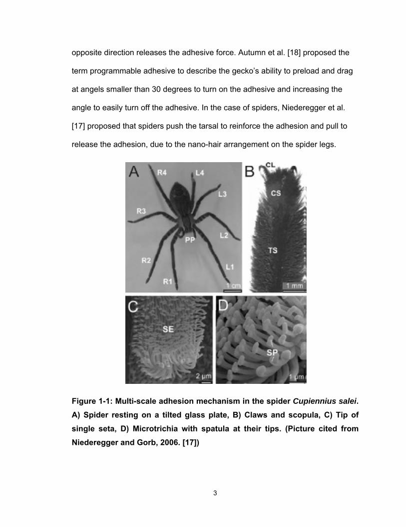
One of the first reported climbing robots successfully implemented with

synthetic dry adhesives was the Mini-WhegTM [9] (Figure 1-2 (a)). Later on, a

climbing robot, Waalbot, with a similar climbing strategy was reported by Murphy

[12] (Figure 1-2 (b)). Both of the robots use wheels with some adhesive pads

attached. The idea behind these climbing robots is to use a simple mechanism to

achieve preloading and peeling for attaching and detaching the adhesive. The

advantage of the wheel design is that the motors required for driving are small

and, therefore, the weight and size of the robot decrease significantly. However,

the disadvantages include: a) the need for a ‘tail’ to preload the adhesive, or else

the robot will flip over and fall down; b) steering difficulties, e.g. turning locally; c)

the wheels are only able to run on continuous trail (i.e., could not overcome

gaps); d) no active control of the direction of attaching and detaching adhesive as

they are predefined by the geometry of the wheel. Waalbot is reported to be able

to climb on vertical surfaces at a velocity of 6 mm/s, and is capable of turning and

transiting between vertical and horizontal surfaces, but the transition is not robust

as it can get stuck in corners.

5

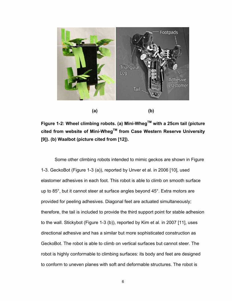
(a) (b)

Figure 1-2: Wheel climbing robots. (a) Mini-WhegTM with a 25cm tail (picture cited from website of Mini-WhegTM from Case Western Reserve University [9]). (b) Waalbot (picture cited from [12]).

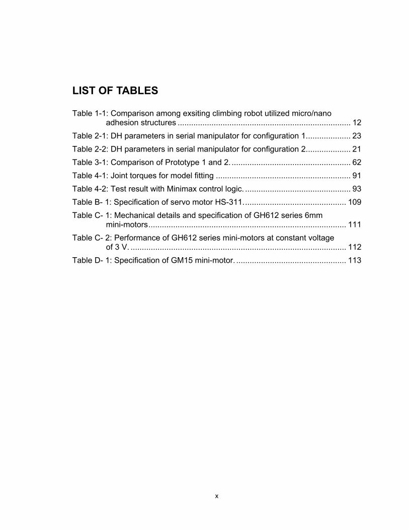
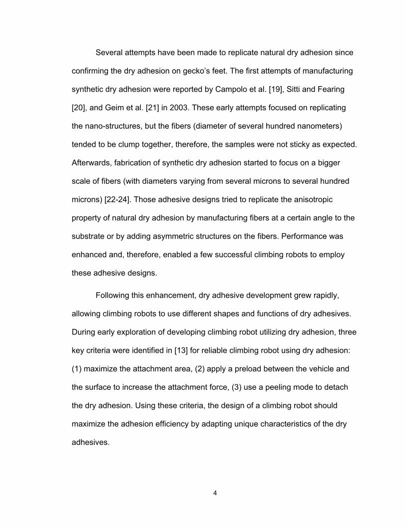
Some other climbing robots intended to mimic geckos are shown in Figure

1-3. GeckoBot (Figure 1-3 (a)), reported by Unver et al. in 2006 [10], used

elastomer adhesives in each foot. This robot is able to climb on smooth surface

up to 85°, but it cannot steer at surface angles beyond 45°. Extra motors are

provided for peeling adhesives. Diagonal feet are actuated simultaneously;

therefore, the tail is included to provide the third support point for stable adhesion

to the wall. Stickybot (Figure 1-3 (b)), reported by Kim et al. in 2007 [11], uses

directional adhesive and has a similar but more sophisticated construction as

GeckoBot. The robot is able to climb on vertical surfaces but cannot steer. The

robot is highly conformable to climbing surfaces: its body and feet are designed

to conform to uneven planes with soft and deformable structures. The robot is

6

under-actuated, having 38 degrees of freedom (DOF) but only actively controlled

by 12 servo motors. Each toe is embedded with a steel string, which is pulled by

an extra servo motor, causing a peeling movement. However, the adhesive

constrained its ability on climbing smooth surfaces. Its ability to steer and transit

is also limited by its design.

7

(a)

(b)

Figure 1-3: Gecko-inspired robots. (a) GeckoBot (picture cited from [10]). (b) StickyBot (picture cited from [11]).

8

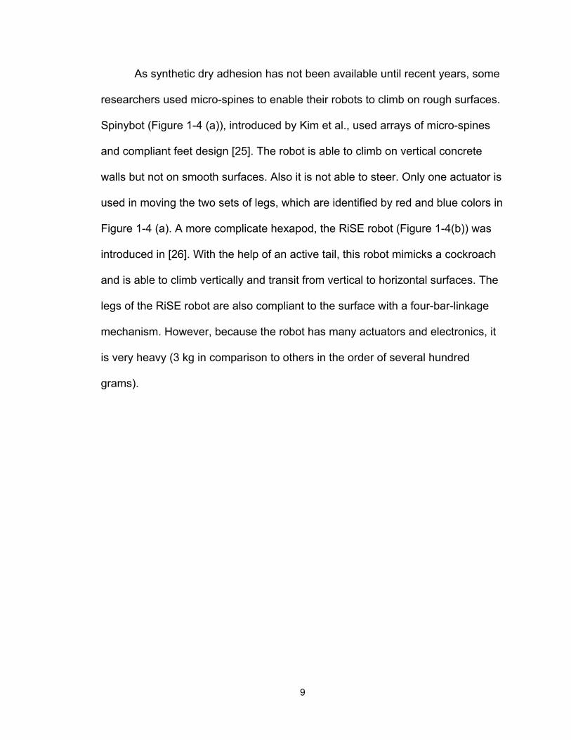
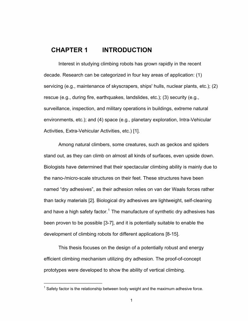
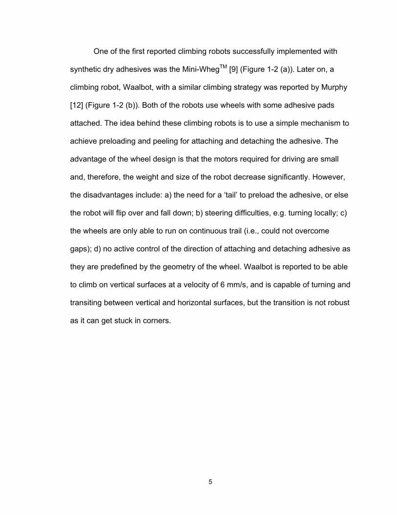
As synthetic dry adhesion has not been available until recent years, some

researchers used micro-spines to enable their robots to climb on rough surfaces.

Spinybot (Figure 1-4 (a)), introduced by Kim et al., used arrays of micro-spines

and compliant feet design [25]. The robot is able to climb on vertical concrete

walls but not on smooth surfaces. Also it is not able to steer. Only one actuator is

used in moving the two sets of legs, which are identified by red and blue colors in

Figure 1-4 (a). A more complicate hexapod, the RiSE robot (Figure 1-4(b)) was

introduced in [26]. With the help of an active tail, this robot mimicks a cockroach

and is able to climb vertically and transit from vertical to horizontal surfaces. The

legs of the RiSE robot are also compliant to the surface with a four-bar-linkage

mechanism. However, because the robot has many actuators and electronics, it

is very heavy (3 kg in comparison to others in the order of several hundred

grams).

9

(a)

(b)

Figure 1-4: Spine embedded climbing robots. (a) SpinyBot and a close-up of the foot (Pictures cited from [25]). (b) the RiSE robot climbing on a tree (upper-left), close-up of foot (upper-right) and compliant foot design (lower). (Picture cited from [26]).

10

11

By investigating most of the existing climbing robots, including those

introduced above, no existing general climbing machine can achieve versatile

tasks. Successful climbing robots are designed for specific tasks, e.g., cleaning

windows, climbing on ferrous flat surfaces, climbing inside or outside of tubes for

inspection. The existing robots are unable to climb on other surfaces than those

they were originally designed for. Upon encountering unexpected surfaces, (e.g.,

convex, gaps, or obstacles) the robot will fail to stick to the wall which may result

in fatal damage. The performance of the robots previously introduced

summarized in Table 1-1. The research in this thesis is to develop a climbing

robot that can potentially overcome the limitation of existing robots.

Table 1-1: Comparison among exsiting climbing robot that use micro/nano adhesion structures

Leg/ wheel

DOF (motor) Tail Weight (g) Size (mm) Surface Steering Transfer Speed

Mini-WhegTM

(PSA2 and dry

adhsion)

Wheel N/A (1) yes

(PSA: no)

76 g (PSA) 110 g/132 g

(dry adhesion, 6.6 cm/25 cm

tail)

54×89 (thickness not

given)

Smooth, 6.6 cm tail – 60°, 25 cm tail – 90°

yes yes

5.8 cm/s (PSA vertical sruface)

8.6 cm/s (dry adhesion 60

deg surface)

Waalbot Wheel N/A (2) yes 69 g 130×50×123 Smooth, up to 110° surface yes

yes, not reliable (stuck in corners)

6 mm/s (straight) 37°/s (steering)

Geckobot Leg 1 (7) yes (100 mm)

100 g 190×110

(exclude tail, thickness not

given)

Smooth, up to 85° surface

yes (no in surface angle 45° )

no 5 cm/s (ground),

4 cm/s (tilt surface)

Stickybot Leg 38 (12) yes 370 g 600×200×60 Smooth, up to 110° surface no no

24 cm/s (ground), 4 cm/s (tilt surface),

Spinybot Leg

(micro-spine)

1 (7) yes 400 g 580×300 (COM to wall: 10 mm) Rough no no 2.3 cm/s (vertical

surface)

RiSE robot Leg

(micro-spine)

12 (12) yes 3000 g 2500 (body

length, others not given)

Rough, 90° on carpet,

55°on wood yes yes

17 cm/s (vertical carpet), 24cm/s (asphalt ground)

2 PSA stands for pressure sensitive adhesion, such as Scotch® tape.

12

1.2 Objective

A successful climbing robot should be able to handle various tasks which

conventional mobile robots cannot achieve. Compared to wheeled robots, legged

robots possess greater mobility, e.g., turning locally and versatility locomoting in

different terrains. By considering the use of dry adhesion for climbing, a legged

robot may be considered to be a preferable solution because of its flexibility of

movement, which could allow changing orientation and direction of the feet to

comply with the anisotropic property of the synthetic dry adhesive.

Randall [27] specified several properties a robot should have to agilely

walk: (1) highly adaptive to environment, (2) lightweight, (3) reliable and robust,

(4) high force to weight ratio, (5) navigate using 3D path planning, (6) possibility

to ‘learn from experience’, (7) have reliable and robust control system to drive

various actuators, (8) be able to sense its environment to achieve tasks

efficiently, and (9) design functions in module in order to ‘plug and play’ in

specific tasks. For a wall-climbing robot, additional requirements are emphasized

to achieve the particular climbing feature. The robot should be able to: (1) transit

between horizontal and vertical surfaces in all directions, (2) negotiate obstacles

and ledges, (3) prevent falling due to occasional adhesion failure, and (4)

maximize adhesion efficiency.

For a climbing machine, the weight and, therefore, miniaturization should

have higher priority than a usual walking machine. Miniaturized robots can also

take advantage of their reduced size to go through narrow spaces for tasks not

13

suitable for bigger robots. The climbing robot, therefore, should be designed to

have compact structures to maintain low body weight and small size.

With millions of years of evolution, spiders, specifically hunting spiders,

survive and thrive with their hunting skills. Compared to geckos, they have a rigid

body and legs instead of flexible muscles and skin; this property is much easier

to mimick in engineering design. The spider adhesion mechanism, which relies

on multi-scale hairs, is compliant to surfaces and can be replicated by synthetic

dry adhesion fabrication technology. With these special properties, spiders are a

preferable bio-mimetic subject for the design of engineering climbing robots.

To summarize, the robot designed in this thesis was designed to: 1) be

miniaturized and lightweight; 2) rely on dry adhesives; and 3) have a legged

configuration. Using solutions found in spiders, the robot in this thesis should be

able to adapt to different surfaces, shapes and materials.

1.3 Thesis outline

The layout of the remaining parts of this thesis is arranged as follows:

Chapter 2 first presents the basic configurations of size, weight, and construction

according to the objective of the research. Thereafter, analyses of the kinematic

properties are performed. Equations are developed to calculate the direct

kinematics and inverse kinematics for legs in swing phase, which is the instant

while the legs are moving in air without touching a fixed base. Inverse kinematic

equations are also used to control the robot body movement. Lastly the local

14

ground coordinate is introduced to further implementation of kinematic equations

while the robot is moving in sequential steps.

Chapter 3 introduces two prototypes developed during this research and

presents their mechatronic design. A comparison between the two prototypes is

discussed.

Chapter 4 demonstrates the validation of the kinematic equations and the

development of simplified control strategies. Tests are performed to determine

the power saving trajectories for the feet to release adhesion in order to make

reliable contact position for reinforced adhesion. Validation of an algorithm, which

was developed in MENRVA Group to reduce reaction force between adhesive

feet and the wall, is performed. Test results are discussed that show actively

controlled joint torques of the robot can reduce significantly the adhesive

requirement.

Chapter 5 proposes future development of an under-actuated system.

Preliminary joint design is introduced and the robotic concept design is

explained. The advantage of an under-actuated system is that it could reduce

robot weight and cost of future platforms.

Chapter 6 presents the conclusion of all the preliminary results and points

out future work towards a fully reliable bio-mimetic climbing robot.

1.4 Thesis contributions

The use of dry adhesion relying on van der Waals forces that are not

constrained by surface materials and shapes opens a new area of research for

15

climbing robot development. The contribution of this thesis is utilizing the

advantages of synthetic dry adhesion to investigate the development of a spider-

inspired robot which possesses the ability to maneuver in different terrains.

Firstly, by considering the different terrains the robot might encounter, a

basic configuration for a climbing robot is proposed. Secondly, kinematic

equations set for the climbing robot are proposed. Assigning coordinates to

control the robot in successive steps is introduced based on kinematic analysis.

Furthermore, with specific application to the climbing robot, the theory of peeling

the thin film is revisited and applied in releasing adhesion. A power saving

trajectory is proposed and proved in a power consumption test. Finally, a robot

prototype is developed that is able to climb a vertical smooth surface with a

synthetic dry adhesive attached. The robot design is validated and the potential

better climbing mechanism is shown as planned.

Overall, the contribution of this work is developing a climbing robot which

has the potential to possess high mobility and the ability to fully utilize the

advantage of dry adhesion.

16

CHAPTER 2 ROBOT DESIGN CONFIGURATIONS AND KINEMATIC ANALYSIS

2.1 Design configurations

In the early design phase, different configurations for the robot design

were analyzed according to the objectives of this research. The synthetic dry

adhesion we had recently fabricated could produce a maximum adhesive force of

around 0.9 kg/cm2 when manually preloaded [28]. Usually, without active

preloading (e.g. pushing the adhesive area by hand), the effective contact area of

the adhesive lowers to 10-20% of the total area. Therefore, the generated

adhesive force was reduced to 100-200 g/cm2. In order to keep the safety factor

of the climbing robot on a reasonable level, we set the maximum weight of the

robot at around 200g and the total adhesive area at around 20 cm2 (a safety

factor at more than 10).

Similarly to spiders, the robot was designed to have multiple legs, which

provide high flexibility to potentially avoid obstacles and walk on rough terrains.

Instead of using eight legs as in spiders, the proposed robot was designed with

six legs in order to reduce its complexity and weight.

In order to enlarge the work-space of each leg and provide high potential

dexterity3 to the robot, a specific configuration was chosen as proposed in Figure

2-1. Three joints were used in each leg. Two of them located at the edge of the

3 Dexterity is the ability of performing tasks.

17

robot platform with cross axes, while the joint in the middle of the leg has a

parallel axis with the second joint. This mechanism is known as an

anthropomorphic arm. The work-space of the anthropomorphic arm is within the

sphere of the full leg length, which means the tip of the leg can reach every point

within a sphere of that size. For the sake of clarity, from the inside out, the three

joints are named the hip, shoulder and elbow joints. Similarly, the second link

(from the shoulder to the elbow joint) is called the femur and the third link (from

the elbow to the end tip of the leg) is called the tibia. The six legs are arranged

60 degrees apart in a circle to better mimick the spider instead of placing them in

two rows as in most engineering hexapods developed so far. The hexagonal

arrangement allows for more gaits and is easier to achieve the desired direction

than the rectangular platform [29]; this configuration could facilitate transition

among perpendicular surfaces. All joints in the six legs were controlled

separately, which guarantees the robot’s dexterity. Based on previous

considerations, the basic configuration of the mechanical design was a 200 g

hexapod having three actuators per leg, with all legs arranged symmetrically

around a circular platform.

18

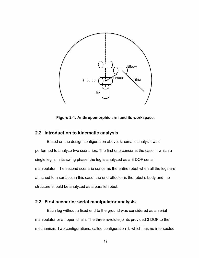
Figure 2-1: Anthropomorphic arm and its workspace.

2.2 Introduction to kinematic analysis

Based on the design configuration above, kinematic analysis was

performed to analyze two scenarios. The first one concerns the case in which a

single leg is in its swing phase; the leg is analyzed as a 3 DOF serial

manipulator. The second scenario concerns the entire robot when all the legs are

attached to a surface; in this case, the end-effector is the robot’s body and the

structure should be analyzed as a parallel robot.

2.3 First scenario: serial manipulator analysis

Each leg without a fixed end to the ground was considered as a serial

manipulator or an open chain. The three revolute joints provided 3 DOF to the

mechanism. Two configurations, called configuration 1, which has no intersected

19

joints axes in the hip and shoulder joints, and configuration 2, which has

intersected joints axes in the hip and shoulder joints, were considered as

presented in the following sections.

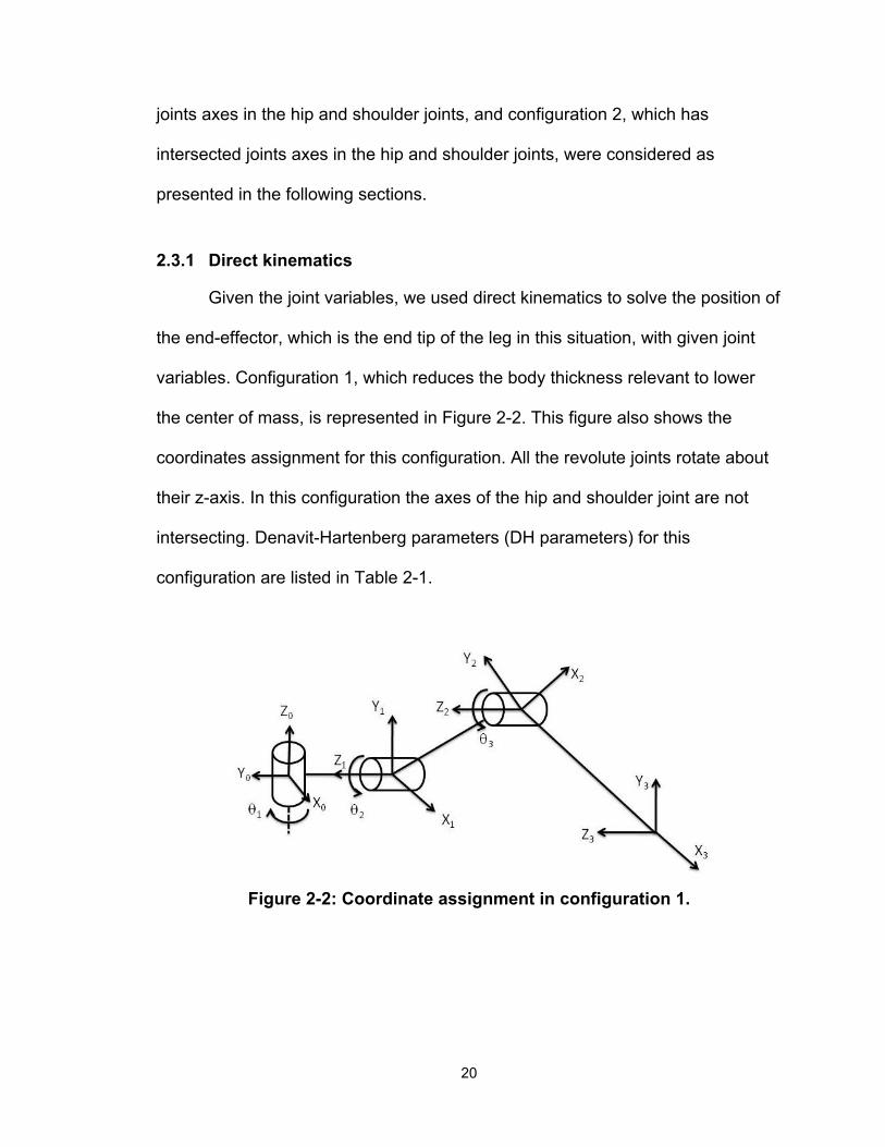
2.3.1 Direct kinematics

Given the joint variables, we used direct kinematics to solve the position of

the end-effector, which is the end tip of the leg in this situation, with given joint

variables. Configuration 1, which reduces the body thickness relevant to lower

the center of mass, is represented in Figure 2-2. This figure also shows the

coordinates assignment for this configuration. All the revolute joints rotate about

their z-axis. In this configuration the axes of the hip and shoulder joint are not

intersecting. Denavit-Hartenberg parameters (DH parameters) for this

configuration are listed in Table 2-1.

Figure 2-2: Coordinate assignment in configuration 1.

20

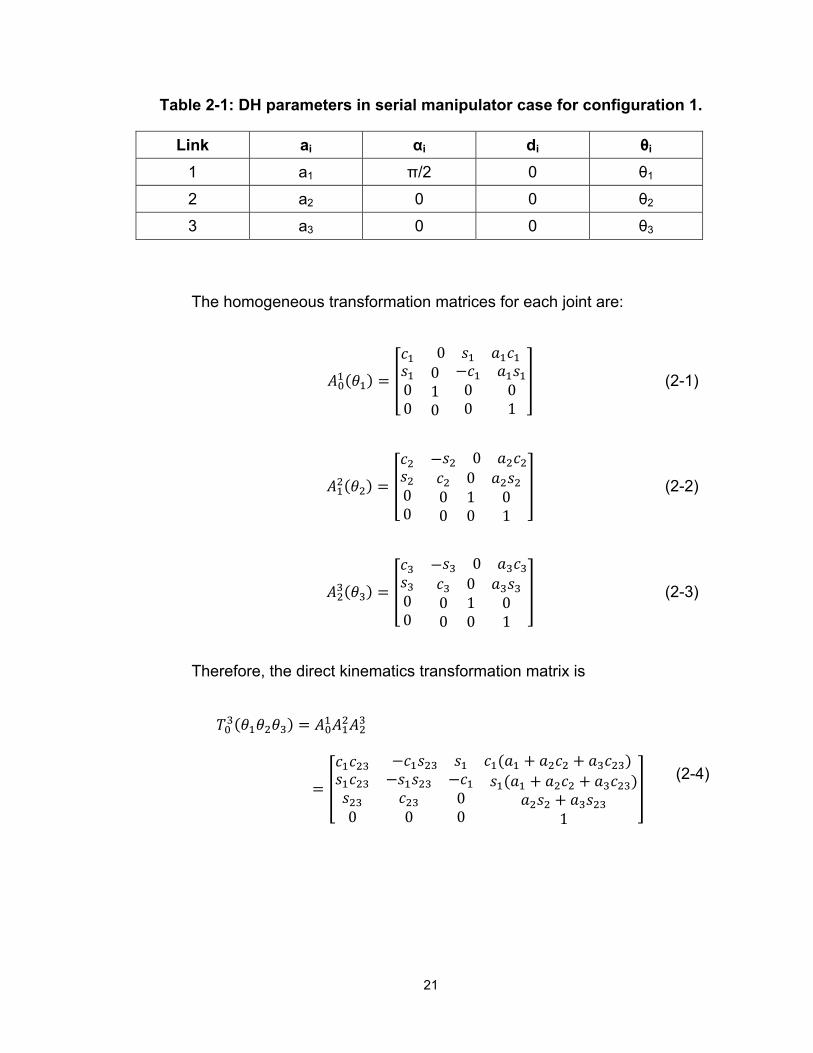
Table 2-1: DH parameters in serial manipulator case for configuration 1.

Link ai αi di θi 1 a1 π/2 0 θ1

2 a2 0 0 θ2

3 a3 0 0 θ3

The homogeneous transformation matrices for each joint are:

0

00

010

00

01

(2-1)

0

00

00 1 00 0 1

(2-2)

0

00

00 1 00 0 1

(2-3)

Therefore, the direct kinematics transformation matrix is

0 000 1

(2-4)

21

With a given set of joint variables, the position of the end-effector is

calculated as a vector with respect to the robot base

, , , ,

(2-5)

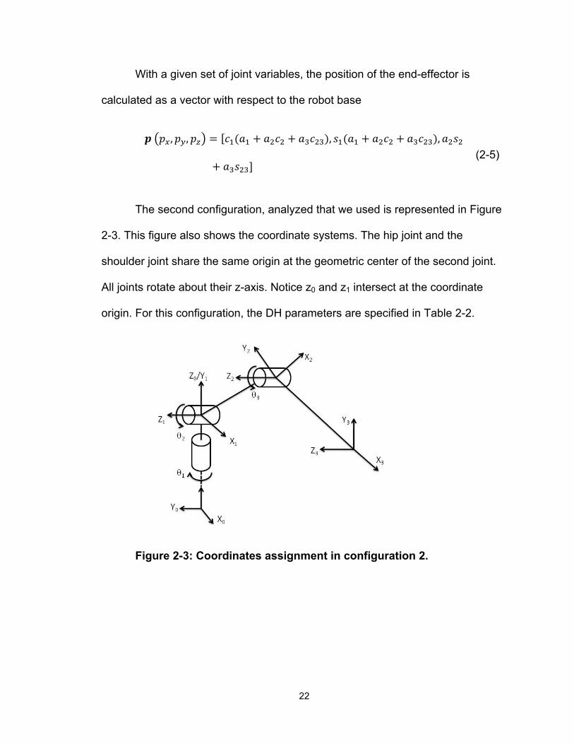
The second configuration, analyzed that we used is represented in Figure

2-3. This figure also shows the coordinate systems. The hip joint and the

shoulder joint share the same origin at the geometric center of the second joint.

All joints rotate about their z-axis. Notice z0 and z1 intersect at the coordinate

origin. For this configuration, the DH parameters are specified in Table 2-2.

Figure 2-3: Coordinates assignment in configuration 2.

22

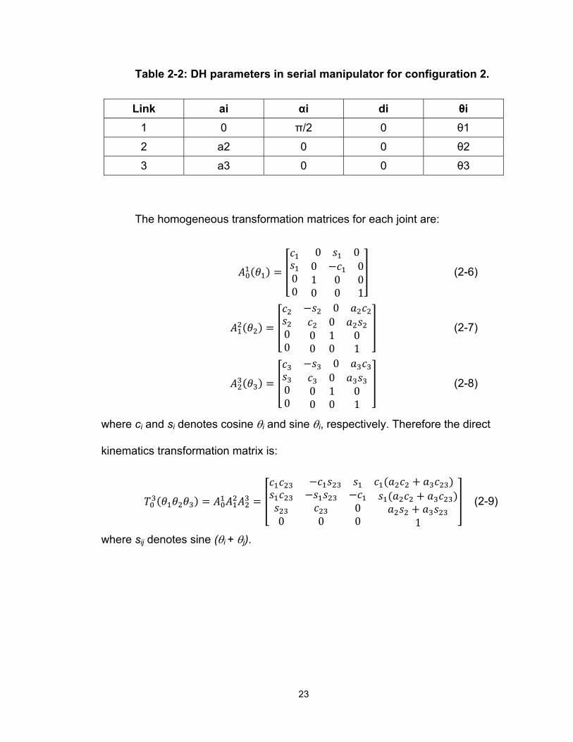
Table 2-2: DH parameters in serial manipulator for configuration 2.

Link ai αi di θi 1 0 π/2 0 θ1

2 a2 0 0 θ2

3 a3 0 0 θ3

The homogeneous transformation matrices for each joint are:

0 0

00

0 0 1 0 00 0 1

(2-6)

00 0

00 1 00 0 1

(2-7)

0

00

00 1 00 0 1

(2-8)

where ci and si denotes cosine θi and sine θi, respectively. Therefore the direct

kinematics transformation matrix i :s

0 000 1

(2-9)

where sij denotes sine (θi + θj).

23

With a given set of joint variables, the position of end-effector is calculated

as a vector with respect to the robot base.

, , , ,

(2-10)

2.3.2 Inverse kinematics

Inverse kinematics is used to solve the set of joint variables when given

the position of the end-effector. In this thesis, the inverse kinematic problem was

solved by geometrical analysis.

Given the end-effector position, vector p (px, py, pz), with respect to the

robot base frame, the hip joint angle was solved directly from vector p, in both

configurations:

(2-11)

Configuration 2 is first discussed for its simplicity. The 2D graph shown in

Figure 2-4 was used for analyzing. The second and third link length is known, as

is the magnitude of the vector p. It should be noticed that there are two

configurations for the same end-effector position (Figure 2-5). According to the

law of cosines, θ3 can be calculated in

2 (2-12)

24

where the negative value physically refers to the elbow up configuration and the

positive value refers to the elbow down configuration.

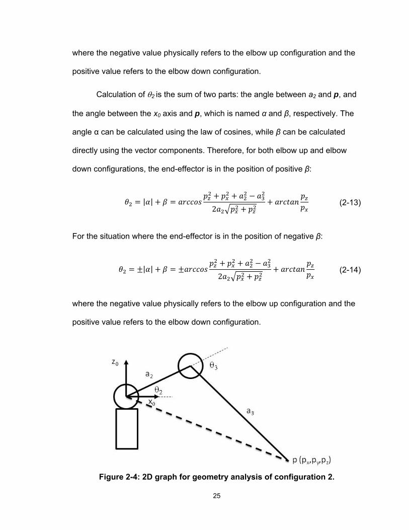
Calculation of θ2 is the sum of two parts: the angle between a2 and p, and

the angle between the x0 axis and p, which is named α and β, respectively. The

angle α can be calculated using the law of cosines, while β can be calculated

directly using the vector components. Therefore, for both elbow up and elbow

down configurations, the end-effector is in the position of positive β:

| |2

(2-13)

For the situation where the end-effector is in the position of negative β:

| |2

(2-14)

where the negative value physically refers to the elbow up configuration and the

positive value refers to the elbow down configuration.

Figure 2-4: 2D graph for geometry analysis of configuration 2.

25

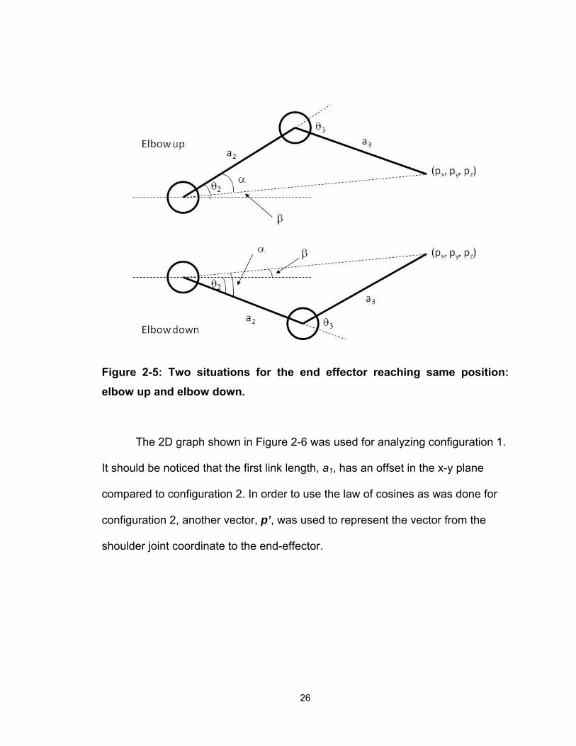
Figure 2-5: Two situations for the end effector reaching same position: elbow up and elbow down.

The 2D graph shown in Figure 2-6 was used for analyzing configuration 1.

It should be noticed that the first link length, a1, has an offset in the x-y plane

compared to configuration 2. In order to use the law of cosines as was done for

configuration 2, another vector, p’, was used to represent the vector from the

shoulder joint coordinate to the end-effector.

26

The relationship between p and p’ is

(2-15)

(2-16)

(2-17)

By using the same approach for configuration 2,

2

(2-18)

where the negative value physically refers to the elbow up configuration and the

positive value refers to the elbow down configuration.

2 (2-19)

The negative value refers elbow up position whereas positive value refers to the

elbow down position.

27

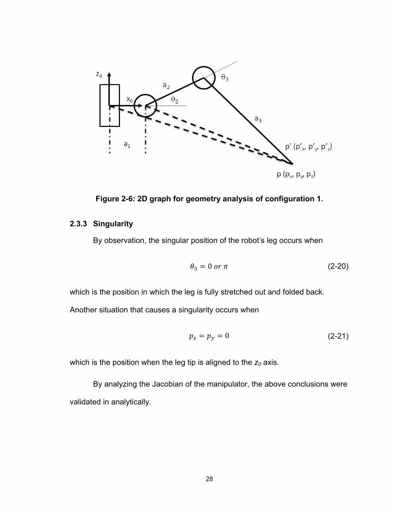
Figure 2-6: 2D graph for geometry analysis of configuration 1.

2.3.3 Singularity

By observation, the singular position of the robot’s leg occurs when

0 (2-20)

which is the position in which the leg is fully stretched out and folded back.

Another situation that causes a singularity occurs when

0 (2-21)

which is the position when the leg tip is aligned to the z0 axis.

By analyzing the Jacobian of the manipulator, the above conclusions were

validated in analytically.

28

The Jacobian is calculated by:

(2-22)

In configuration 1, the position vector of each joint is:

000

(2-23)

0

(2-24)

(2-25)

(2-26)

In configuration 2, the position vector of each joint is:

00 0

(2-27)

(2-28)

(2-29)

29

The unit vector of the revolute axis in each joint, in both prototypes, can be

computed as:

(2-30)

0

(2-31)

For both configurations:

0001 0 0

(2-32)

Only the first three rows are linearly independent, which denotes the

relationship between joint velocity and end-effector linear velocity. Let Jp

represent the first three rows of J. The manipulator does not allow arbitrary

angular velocity because the last three rows of the Jacobian, which represent

angular velocity of the end-effector, are not linearly independent.

30

The determinant of Jp is

det

0

(2-33)

When s3 = 0 or a2c2 + a3c23 = 0, det[Jp] = 0, reaching the singular position. These

are the conditions previously obtained by geometrical inspection.

2.4 Second scenario: parallel platform analysis

For the hexapod robot, the basic requirement for holding the robotic

platform statically stable is having at least three legs contacting the ground (the

robotic ankles are modeled as spherical joints). The attached legs and the robotic

platform then form a parallel manipulator or closed chain mechanism. The body

of the robot becomes the end-effector and it is the object to be controlled.

Therefore, the following analysis focuses on the inverse kinematics of the parallel

configuration presented in Figure 2-7.

31

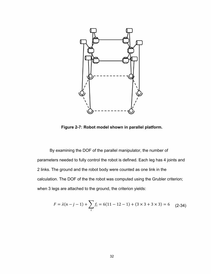
Figure 2-7: Robot model shown in parallel platform.

By examining the DOF of the parallel manipulator, the number of

parameters needed to fully control the robot is defined. Each leg has 4 joints and

2 links. The ground and the robot body were counted as one link in the

calculation. The DOF of the the robot was computed using the Grubler criterion;

when 3 legs are attached to the ground, the criterion yields:

1 6 11 12 1 3 3 3 3 6 (2-34)

32

When 4 legs attach to the ground, the criterion yields:

1 6 14 16 1 4 3 3 4 6 (2-35)

When 5 legs attach to the ground, the criterion yields:

1 6 17 20 1 5 3 3 5 6 (2-36)

And, when 6 legs attach to the ground, the criterion yields:

1 6 20 24 1 6 3 3 6 6 (2-37)

where n denotes the number of links, j denotes the number of joints, λ denotes

dimensions of the moving mechanism. Notice that the calculations always yield

six DOF in all cases.

Above calculation proved that when at least 3 legs are attached to the

ground, the parallel manipulator will always have 6 DOF, which means 6

independent parameters are required as input to control its position. The six

parameters representing six DOF were designed to be (px, py, pz, α, β, γ), where

(px, py, pz) denote the three coordinates of vector p, while α, β, γ denote the Euler

angle controlling the orientation of the robotic platform with respect to the ground.

In order to investigate the inverse kinematics of the platform, the robot

was simplified by replacing the elbow joint by a prismatic joint. The variable

associated with the prismatic joint is presented as di (i=1, 2, 3, 4, 5, 6). By

33

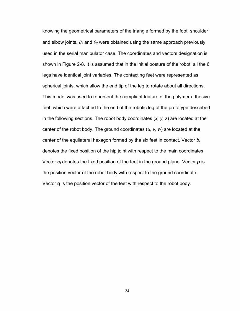
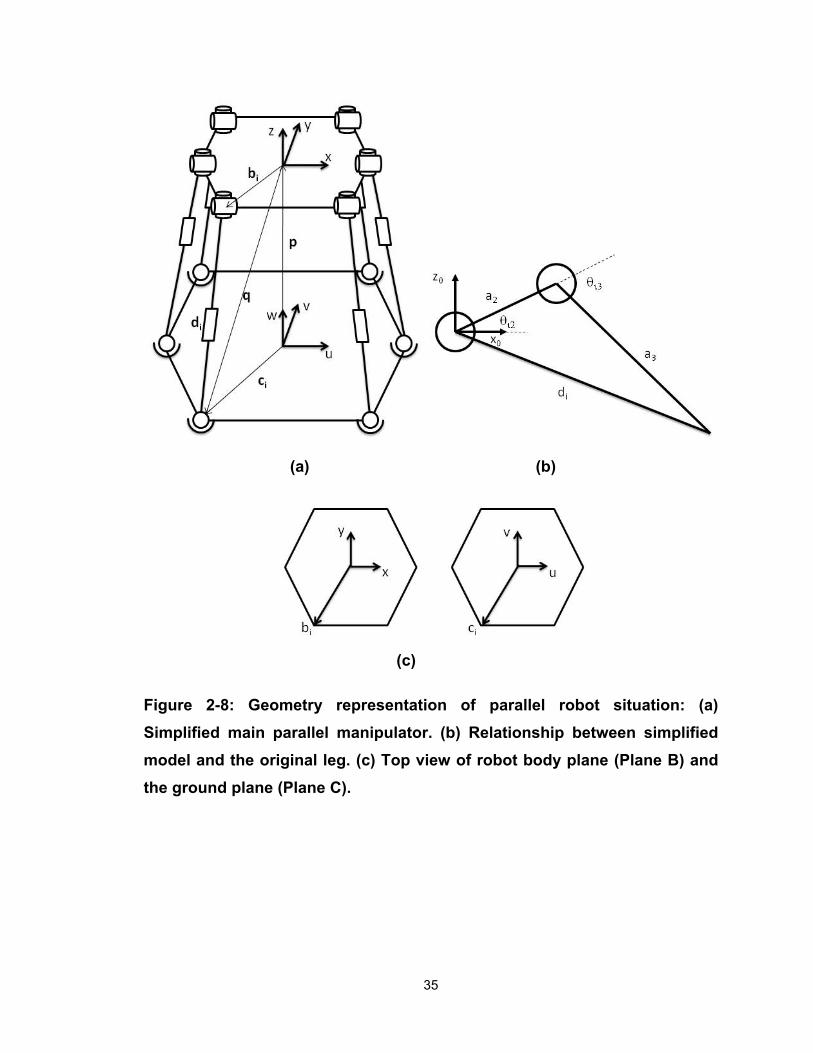
knowing the geometrical parameters of the triangle formed by the foot, shoulder

and elbow joints, θ3 and θ2 were obtained using the same approach previously

used in the serial manipulator case. The coordinates and vectors designation is

shown in Figure 2-8. It is assumed that in the initial posture of the robot, all the 6

legs have identical joint variables. The contacting feet were represented as

spherical joints, which allow the end tip of the leg to rotate about all directions.

This model was used to represent the compliant feature of the polymer adhesive

feet, which were attached to the end of the robotic leg of the prototype described

in the following sections. The robot body coordinates (x, y, z) are located at the

center of the robot body. The ground coordinates (u, v, w) are located at the

center of the equilateral hexagon formed by the six feet in contact. Vector bi

denotes the fixed position of the hip joint with respect to the main coordinates.

Vector ci denotes the fixed position of the feet in the ground plane. Vector p is

the position vector of the robot body with respect to the ground coordinate.

Vector q is the position vector of the feet with respect to the robot body.

34

(a) (b)

(c)

Figure 2-8: Geometry representation of parallel robot situation: (a) Simplified main parallel manipulator. (b) Relationship between simplified model and the original leg. (c) Top view of robot body plane (Plane B) and the ground plane (Plane C).

35

The rotation matrix of the robot’s body coordinates with respect to the

ground coordinates is

(2-38)

Vector qi is calculated by

(2-39)

Then vector di is known by

(2-40)

The magnitude of di is

| | (2-41)

The first variable is given by

arctandd arctan

bb (2-42)

where diy and dix denote the second and first number representing the y and x

axes in vector di, respectively.

36

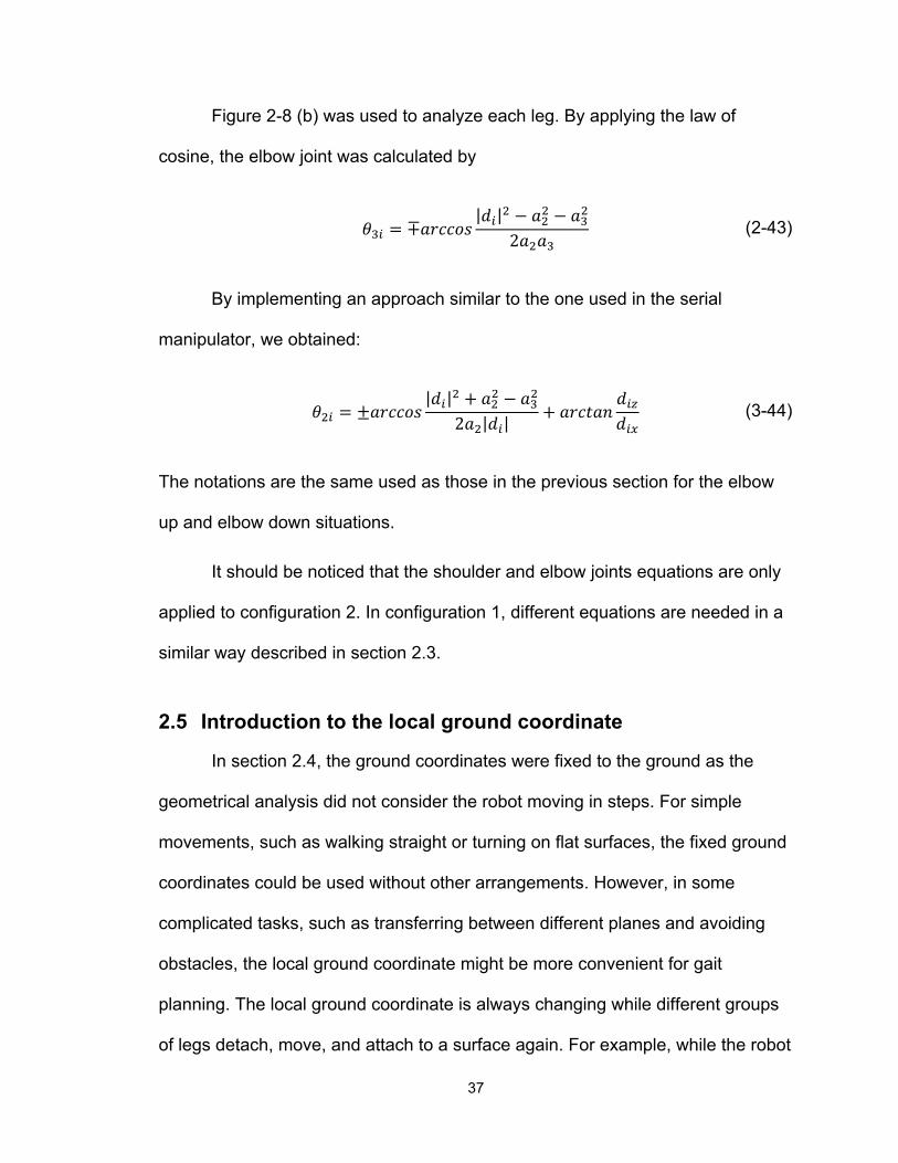
Figure 2-8 (b) was used to analyze each leg. By applying the law of

cosine, the elbow joint was calculated by

| |

2 (2-43)

By implementing an approach similar to the one used in the serial

manipulator, we obtained:

| |

2 | | (3-44)

The notations are the same used as those in the previous section for the elbow

up and elbow down situations.

It should be noticed that the shoulder and elbow joints equations are only

applied to configuration 2. In configuration 1, different equations are needed in a

similar way described in section 2.3.

2.5 Introduction to the local ground coordinate

In section 2.4, the ground coordinates were fixed to the ground as the

geometrical analysis did not consider the robot moving in steps. For simple

movements, such as walking straight or turning on flat surfaces, the fixed ground

coordinates could be used without other arrangements. However, in some

complicated tasks, such as transferring between different planes and avoiding

obstacles, the local ground coordinate might be more convenient for gait

planning. The local ground coordinate is always changing while different groups

of legs detach, move, and attach to a surface again. For example, while the robot

37

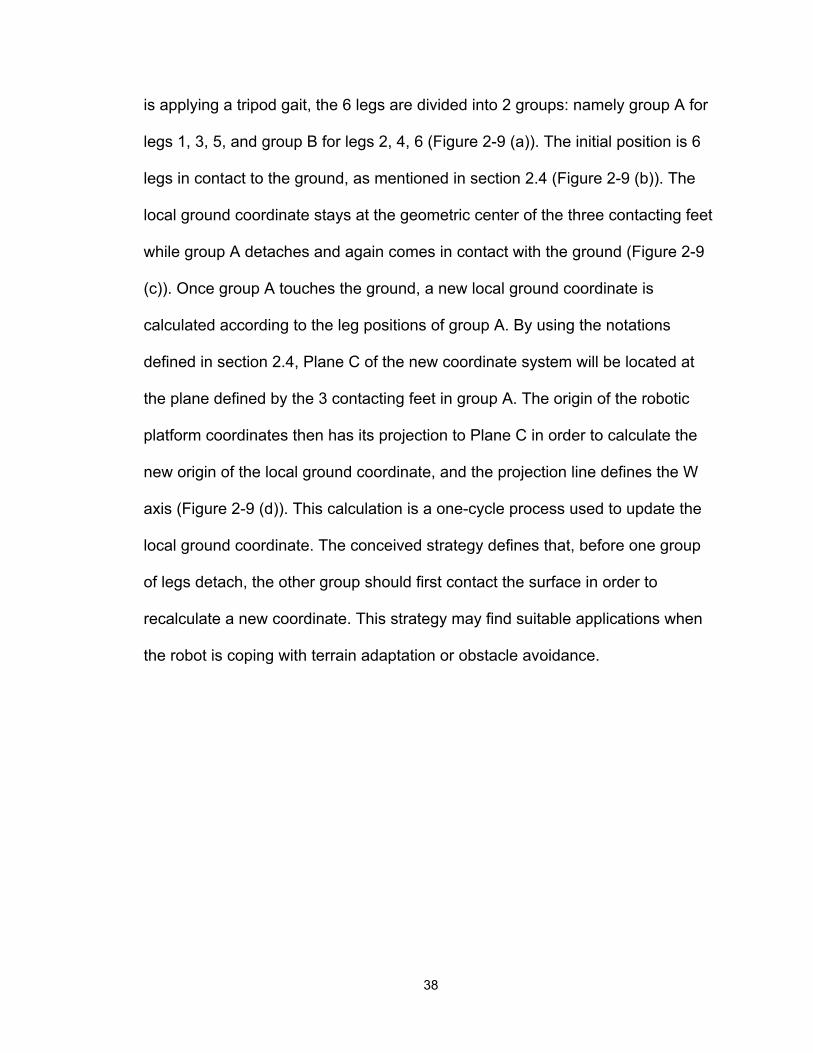
is applying a tripod gait, the 6 legs are divided into 2 groups: namely group A for

legs 1, 3, 5, and group B for legs 2, 4, 6 (Figure 2-9 (a)). The initial position is 6

legs in contact to the ground, as mentioned in section 2.4 (Figure 2-9 (b)). The

local ground coordinate stays at the geometric center of the three contacting feet

while group A detaches and again comes in contact with the ground (Figure 2-9

(c)). Once group A touches the ground, a new local ground coordinate is

calculated according to the leg positions of group A. By using the notations

defined in section 2.4, Plane C of the new coordinate system will be located at

the plane defined by the 3 contacting feet in group A. The origin of the robotic

platform coordinates then has its projection to Plane C in order to calculate the

new origin of the local ground coordinate, and the projection line defines the W

axis (Figure 2-9 (d)). This calculation is a one-cycle process used to update the

local ground coordinate. The conceived strategy defines that, before one group

of legs detach, the other group should first contact the surface in order to

recalculate a new coordinate. This strategy may find suitable applications when

the robot is coping with terrain adaptation or obstacle avoidance.

38

Figure 2-9: Local ground coordinate example: (a) Leg grouping in tripod gait. (b)-(d) Side view interpretation for one cycle of changing the local ground coordinate (consider only group A in this step).

2.6 Chapter conclusion

In this chapter, the basic configuration of the robot was proposed. A

kinematic analysis was, thereafter, performed by considering two configurations

for the position of the leg’s joints. By applying direct kinematic equations for each

leg, the position of the feet was mapped and used for calculating the robot

position with respect to the ground coordinate. By utilizing inverse kinematic

equations, it is possible to plan the motion of the robot to walk, climb and cope

with obstacles. In the following chapter, these equations are used to generate

position data for the robot walking in a pentapedal gait.

39

CHAPTER 3 MECHANICAL AND MECHATRONIC DESIGN

Based on the analysis presented in Chapter 2, two prototypes were

developed by considering the two configurations of the position of the leg’s joints,

which affect the thickness of the robot’s body. A smaller body thickness is

assumed to be better because the center of mass (COM) of the robot’s body,

which houses most of the electronics and has most of the robot weight, can be

placed closer to the contacting wall. With the COM closer to the wall, the torque

generated by body weight with respect to the adhesive feet is reduced, avoiding

twisting on the synthetic dry adhesive, which can cause adhesion failure. On the

other side, the configuration 1, in which the shoulder and the elbow joints are

yields a more compact robot.

In this chapter, the mechatronic design of two prototypes, respectively

having configuration 1 and 2, are introduced. Discussion about their performance

is given in Chapter 4.

3.1 Manufacturing of robot construction part

A rapid prototyping machine, InVisionTM HR Si2 3-D Printer, was used in

all the prototype manufacturing. Parts were designed in SolidWorks and sent to

the printer for fabrication. The machine allows new prototype fabrication within

one day and achieves relatively good accuracy, which is important for a

miniaturized robot. From a test of gap printing, the minimum clearance the

40

machine achieves is 0.25 mm. The disadvantage of this machine is the part

material, VisiJet® SR-200, is made from triethylene glycol dimethacrylate ester

and urethane acrylate polymer, which is brittle and can be easily broken by

applying large forces. The material properties require that the mechanical design

should avoid large forces acting on the weak parts. Specification of the part

material is given in [49].

3.2 Prototype 1: hexapod using servo motor electronics

3.2.1 Mechatronic system analysis

Prototype 1 was designed according to configuration 1, which confers the

prototype a smaller body thickness (Figure 3-1). To control a robot walking as

planned, a position control was implemented, using a position sensor, an

actuator, and a controller. Towards this objective, a servo motor was used, as it

contains all these components.

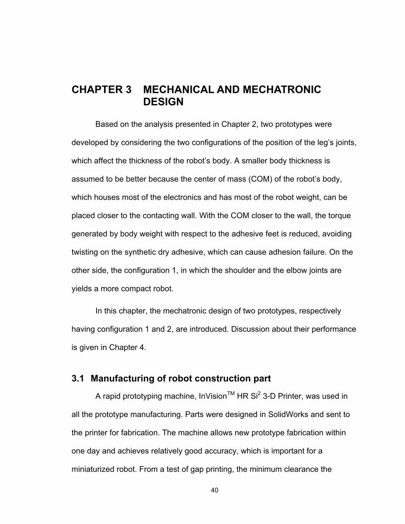
Some parts from the servo motors, Hitec HS-311, were used in this first

prototype (Appendix B). A typical servo motor contains a gearbox, a DC motor, a

potentiometer, and a preprogrammed Printed Circuit Board (PCB), which form

the closed loop control of a joint (Figure 3-2). The preprogrammed PCB consists

of the electronics for controlling the position of the servo motor. From the servo

controller, the position signal (in angles) is sent to the preprogrammed PCB to

run the motor until the potentiometer reaches the set point value. Three wires

attach to the servo motor: a signal line and two power lines. The signal line is

41

receiving signals in pulses, while the power lines provide power to the motor in a

constant voltage level.

(a) (b)

(c)

Figure 3-1: Design of Prototype 1. (a) CAD model of one leg in Prototype 1. (b) CAD model of Prototype 1. Blue part represents the motor, green part denotes the preprogrammed PCB and grey part is the robot construction part manufactured by the 3D printer. (c) Prototype 1 without servo controller.

42

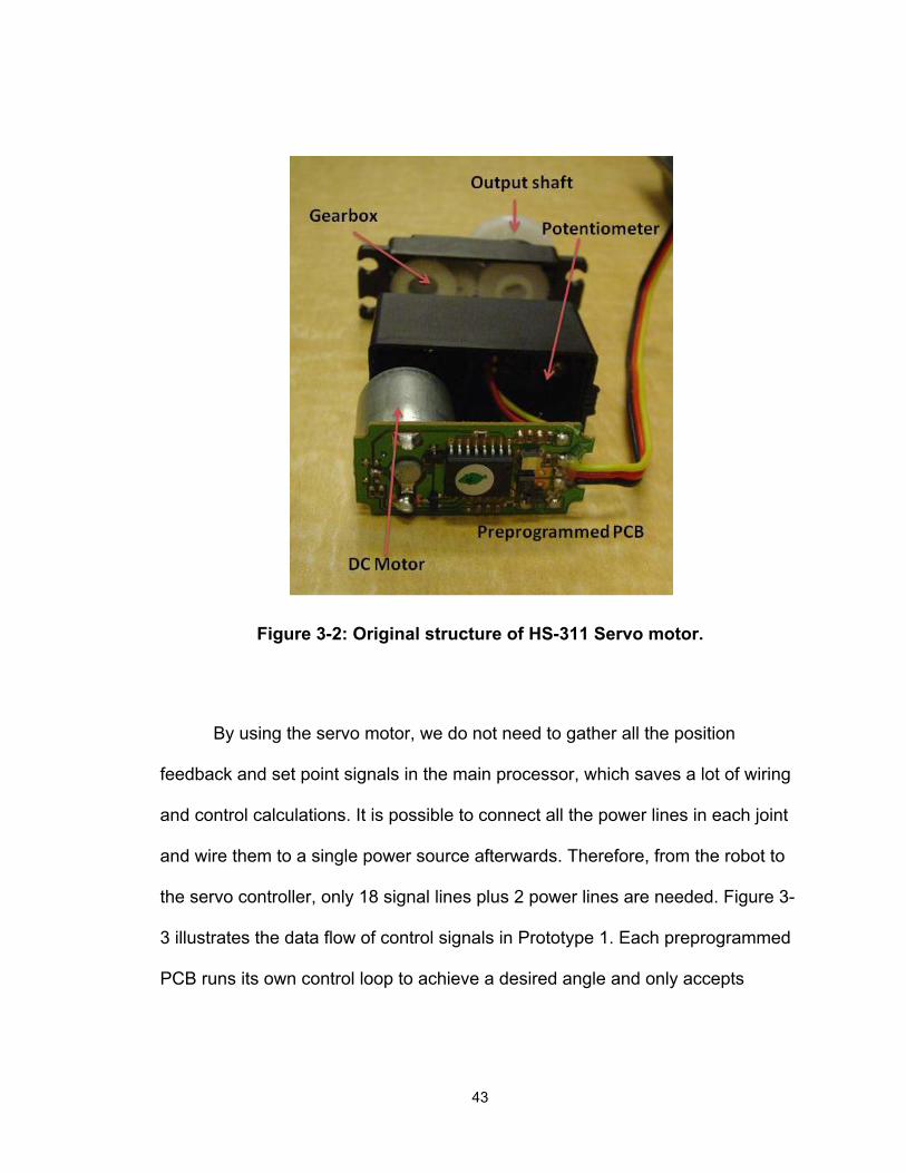
Figure 3-2: Original structure of HS-311 Servo motor.

By using the servo motor, we do not need to gather all the position

feedback and set point signals in the main processor, which saves a lot of wiring

and control calculations. It is possible to connect all the power lines in each joint

and wire them to a single power source afterwards. Therefore, from the robot to

the servo controller, only 18 signal lines plus 2 power lines are needed. Figure 3-

3 illustrates the data flow of control signals in Prototype 1. Each preprogrammed

PCB runs its own control loop to achieve a desired angle and only accepts

43

position signals from the servo controller. Position signals are stored in the

computer and sent to the servo controller by controlling software.

Figure 3-3: Data flow of Prototype 1.

3.2.2 Mechanical structure of modified servo joint

In order to take advantage of the servo motor’s electronics while still

maintaining the miniature feature of the robot, a 6 mm DC motor attached with a

mini gearbox from Gizmo’s Zone (GH6124S, Appendix C) replaced the original

gear box and motor. The gear ratio of the attached gearbox is 1:699.55. Figure 3-

1 (a) and (b) shows the CAD model of a leg and the robot prototype; (c) shows

the final prototype without the servo controller board. The potentiometer

constituted the joint and the PCB was integrated as part of the leg stem. Figure

44

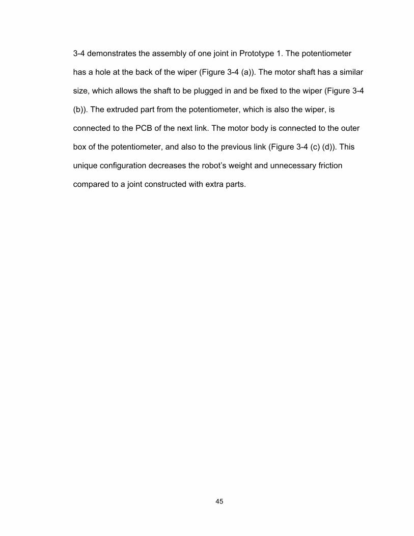
3-4 demonstrates the assembly of one joint in Prototype 1. The potentiometer

has a hole at the back of the wiper (Figure 3-4 (a)). The motor shaft has a similar

size, which allows the shaft to be plugged in and be fixed to the wiper (Figure 3-4

(b)). The extruded part from the potentiometer, which is also the wiper, is

connected to the PCB of the next link. The motor body is connected to the outer

box of the potentiometer, and also to the previous link (Figure 3-4 (c) (d)). This

unique configuration decreases the robot’s weight and unnecessary friction

compared to a joint constructed with extra parts.

45

(a) (b) (c)

(d)

Figure 3-4: Assembly of one joint in Prototype 1. (a) Back of the potentiometer. (b) Motor shaft plugged in the rotor of the potentiometer. White part is the gearbox. (c) A joint assembly on Prototype 1. (d) Assembly structure of one joint.

46

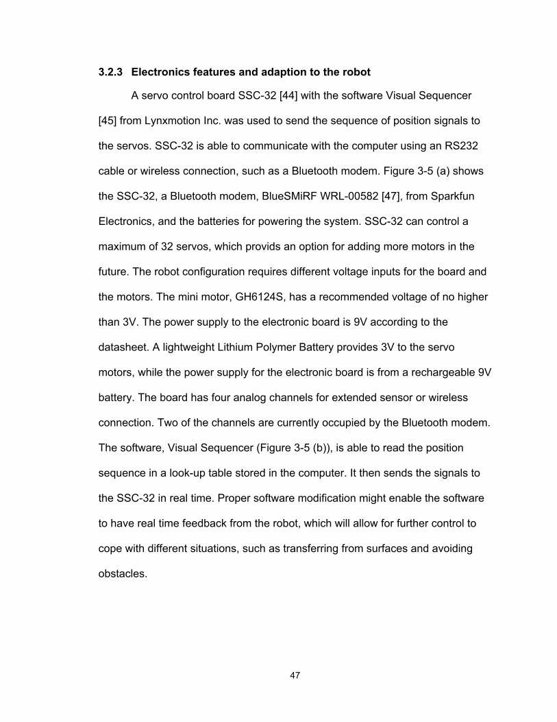
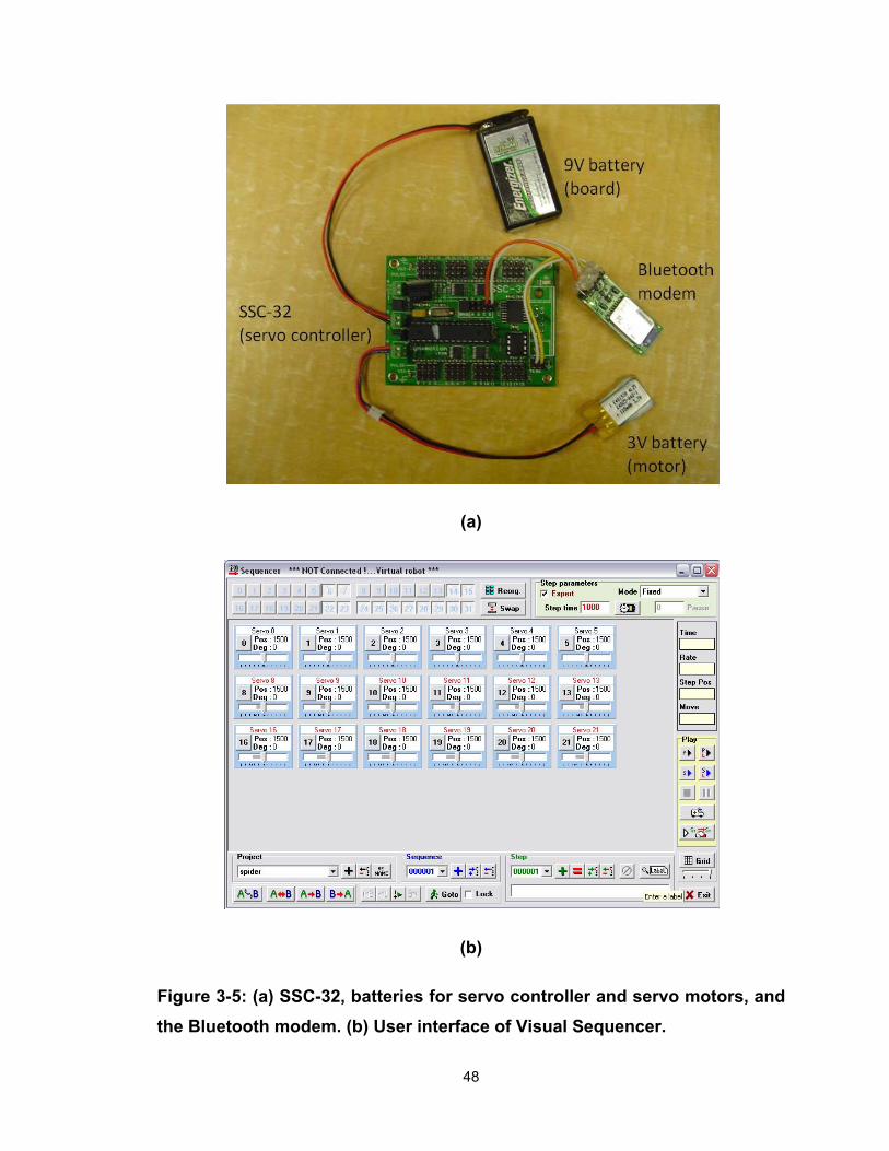
3.2.3 Electronics features and adaption to the robot

A servo control board SSC-32 [44] with the software Visual Sequencer

[45] from Lynxmotion Inc. was used to send the sequence of position signals to

the servos. SSC-32 is able to communicate with the computer using an RS232

cable or wireless connection, such as a Bluetooth modem. Figure 3-5 (a) shows

the SSC-32, a Bluetooth modem, BlueSMiRF WRL-00582 [47], from Sparkfun

Electronics, and the batteries for powering the system. SSC-32 can control a

maximum of 32 servos, which provids an option for adding more motors in the

future. The robot configuration requires different voltage inputs for the board and

the motors. The mini motor, GH6124S, has a recommended voltage of no higher

than 3V. The power supply to the electronic board is 9V according to the

datasheet. A lightweight Lithium Polymer Battery provides 3V to the servo

motors, while the power supply for the electronic board is from a rechargeable 9V

battery. The board has four analog channels for extended sensor or wireless

connection. Two of the channels are currently occupied by the Bluetooth modem.

The software, Visual Sequencer (Figure 3-5 (b)), is able to read the position

sequence in a look-up table stored in the computer. It then sends the signals to

the SSC-32 in real time. Proper software modification might enable the software

to have real time feedback from the robot, which will allow for further control to

cope with different situations, such as transferring from surfaces and avoiding

obstacles.

47

(a)

(b)

Figure 3-5: (a) SSC-32, batteries for servo controller and servo motors, and the Bluetooth modem. (b) User interface of Visual Sequencer.

48

3.2.4 Robot performance

Prototype 1 was able to synchronize all 18 joints to follow the position

sequences in order to achieve the designed movements. The total robot weight

was around 260 grams, including all the batteries, electronics and

communication parts. The length of the robot body was 90 mm and leg length

was 100 mm. Maximum output torque from each joint is 2×10-2 N·m by using a

3V power supply which powers the motors. The robot was able to walk straight

and turn with different gaits on horizontal surfaces, and it was also able to climb

on smooth surfaces up to 90 degrees (i.e., vertical wall) with adhesives attached.

Several issues observed during the tests, should be addressed: (1) due to

clearances among gears in the motor gearbox, the joint have approximately three

to five degrees of error. Both the gears and the motor shaft are fabricated with

Glass Fiber Reinforced Engineering Plastic; with increasing load, especially

when the robot climbs and uses adhesives, the clearance increases and

eventually strips the teeth of the gears, sometimes even breaking the motor

shaft. No substitute product has been found to date. (2) A lack of documentation

about the preprogrammed PCB from the servo motor resulted in difficulties in

accurately positioning the motor. From our observations, the controller on the

PCB might be a simple Proportional-Integral-Derivative (PID) controller which

has parameters that are not specified in the datasheet. The PIC manufactured by

Hitec has no part numbers, and the controller parameters are neither accessible

nor changeable. A digital servo, HS-5475HB, from Hitec, which is programmable

by a digital servo programmer (Hitec HFP-20), was also tested with different

49

dead-band widths. No distinct enhancement of accuracy was observed in

comparison to the analog servo HS-311. (3) The movement of the robot was not

very smooth, especially when the leg is in its swing phase. This problem is not

major, but it might be one of the reasons causing unstable movement. (4) The

large number of wires from the servo-motors accounts for more than 20% of the

robot weight. By examining the weight of one joint, the signal and power wires

are 3.1 g and all other parts including the PCB, motor, and potentiometer weight,

only weigh 5.0 g. A solution to this problem was found by substituting the existing

thick wires with thin silver wires (0.0762 mm bare Teflon coated silver wire from

A-M Systems); the modified servo motor in fact performed as good as the original

one with respect to both reaction speed and output torque.

3.3 Prototype 2: hexapod with motor driven joints

Prototype 2 was designed to have fully customized electronics and

mechanical structure (Figure 3-6). The prototype was designed using

configuration 2 in the kinematic analysis. Compared to Prototype 1, this prototype

was designed with all parts specifically selected, resulting in a more compact

structure. The weight of Prototype 2 was around 130 g without a battery, nearly

half of the mass of Prototype 1 which was 260 g. Electronic boards were stacked

in three layers in the middle of the robot body. In this prototype, the joint was

fabricated from the 3D printer material, instead of using the rotation mechanism

of the potentiometer as in Prototype 1. Magneto-sensitive sensors were used as

position feedback and placed beside the joints without touching the motor.

Actuators and sensors located at the joint formed a compact and clean structure

50

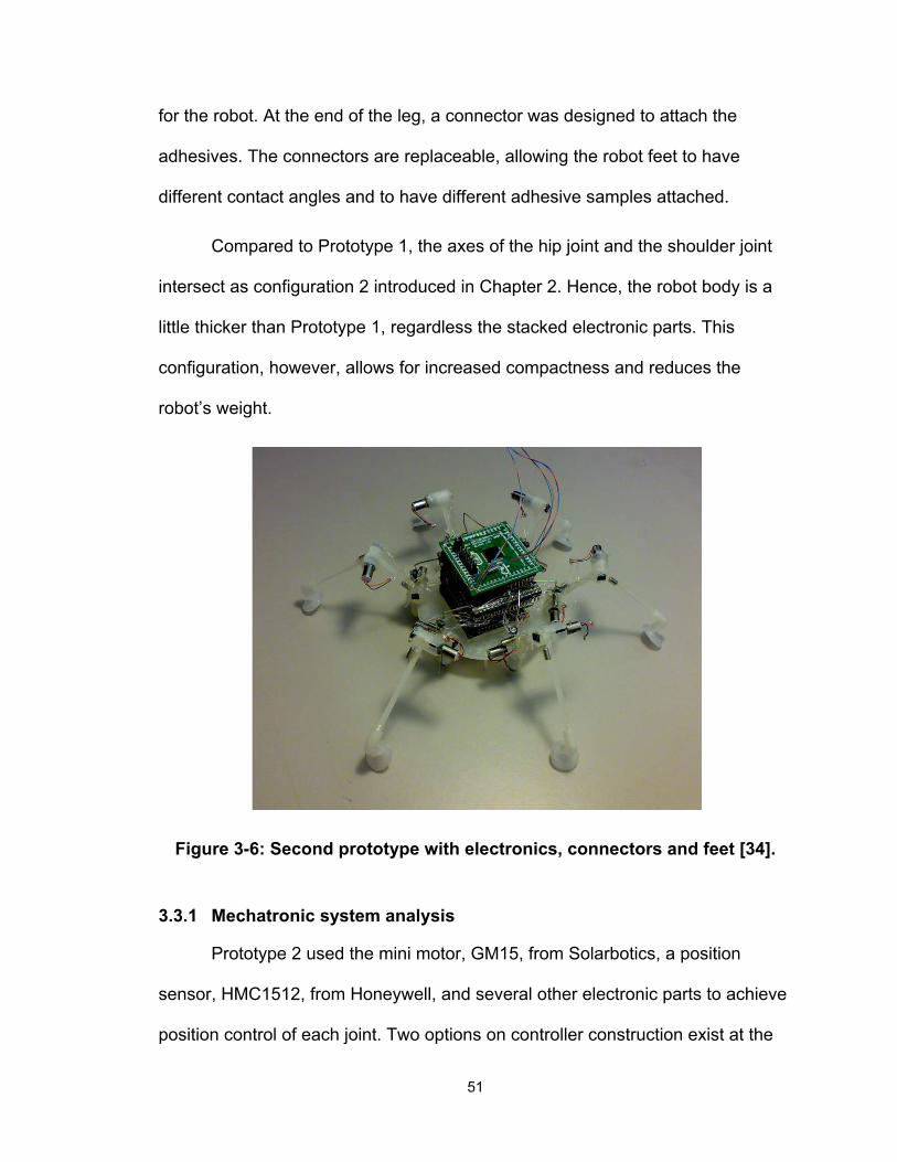
for the robot. At the end of the leg, a connector was designed to attach the

adhesives. The connectors are replaceable, allowing the robot feet to have

different contact angles and to have different adhesive samples attached.

Compared to Prototype 1, the axes of the hip joint and the shoulder joint

intersect as configuration 2 introduced in Chapter 2. Hence, the robot body is a

little thicker than Prototype 1, regardless the stacked electronic parts. This

configuration, however, allows for increased compactness and reduces the

robot’s weight.

Figure 3-6: Second prototype with electronics, connectors and feet [34].

3.3.1 Mechatronic system analysis

Prototype 2 used the mini motor, GM15, from Solarbotics, a position

sensor, HMC1512, from Honeywell, and several other electronic parts to achieve

position control of each joint. Two options on controller construction exist at the

51

beginning of electronic design: an onboard micro controller or an off-line

computer transferring signals via wireless connection to the onboard electronics.

This thesis will only discusses the off-line computer controller designed using

LabVIEW from National Instruments (NI).

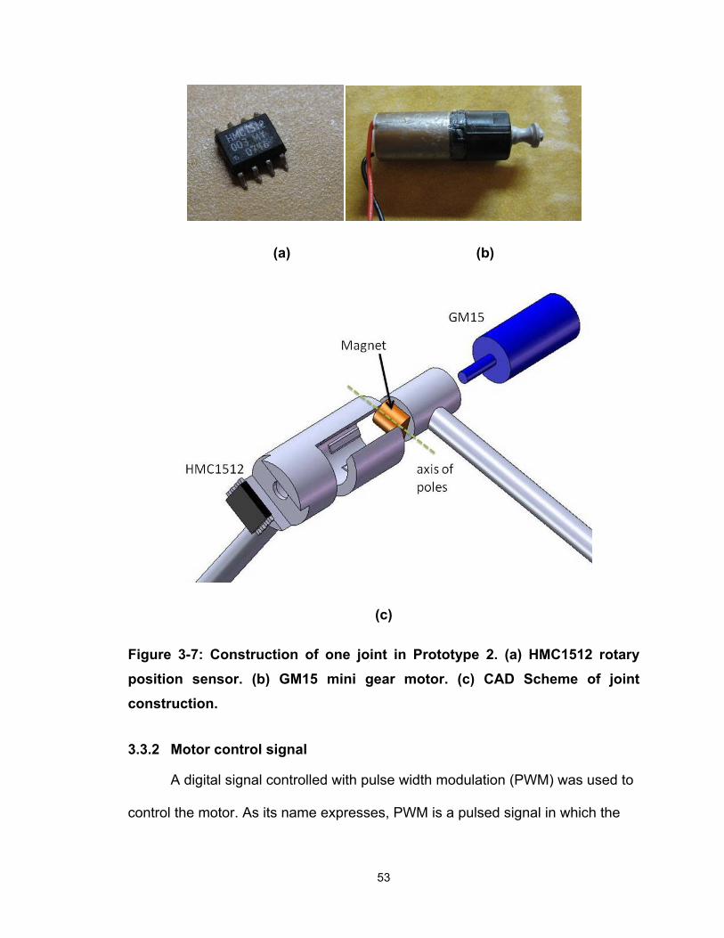
The position sensor HMC1512 (see Figure 3-7 (a)) was selected because

it is frictionless compared to a typical position sensor such as potentiometers.

The size of the chip is 5 mm × 5 mm ×1 mm and each weighs 5 g. The resolution

of the sensor is approximately 0.05 degree [39]. It has 8 pins: 4 power pins and 4

signal pins from 2 Wheatstone Bridges. Differentiations of the 4 signal outputs

form the 2 signals from each bridge, which are used in angular position

calculations. GM15 (see Figure 3-7 (b)) was chosen because of its miniaturized

features (6 mm diameter) and because it includes a gearbox (gear ratio 1:25,

Appendix D). The H-bridge chip SN754410 is one of the most common PICs

used for controlling small robots. This chip can control two motors rotating

clockwise (CW) or counter-clockwise (CCW) at the same time. According to the

datasheet, the chip requires only 1 input line for each motor with the simple

circuit with a converter. The input signal to the motors and output signal from the

sensors are analyzed by using a Data Acquisition Card (DAQ) USB-6259 - a

simple PID controller was designed and tested in LabVIEW 8.2. Joint design is

shown in Figure 3-7 (c).

52

(a) (b)

(c)

Figure 3-7: Construction of one joint in Prototype 2. (a) HMC1512 rotary position sensor. (b) GM15 mini gear motor. (c) CAD Scheme of joint construction.

3.3.2 Motor control signal

A digital signal controlled with pulse width modulation (PWM) was used to

control the motor. As its name expresses, PWM is a pulsed signal in which the

53

percentage of the high voltage (5V) in one period, which is called duty cycle,

decides the information in the signal. PWM can also be thought as an average

voltage level, as in an analog signal. To apply PWM to the DC motor, an H-

bridge and converter circuit is usually added between the signal source and the

motor. By applying a 50% duty cycle, the motor receives an ‘average voltage’ of

0V, while a 100% and 0% duty cycle will run the motor in full speed rotating CW

and CCW, respectively. This method solves the problem of the dead-band

caused by the excitation voltage of the motor in the case of an analog signal. The

pulse rotates the motor in two directions with a certain frequency, which

decreases the heat otherwise caused when an analog signal is used in holding

high torque. Test results showed that the minimum frequency of PWM that

should be applied to the circuit is 50 Hz. Frequencies lower than 50 Hz will cause

the motor to oscillate. Usually a 500 Hz PWM is applied to the circuit for smooth

movement.

3.3.3 Sensor selection and tests

For position feedback, the potentiometer is one of the most common

angular sensor used in miniaturized robots. It has the advantage of being

lightweight, having a simple signal output (one line analog signal), and it is

available in a large variety of different shapes and resistances. One main

disadvantage of potentiometers is the friction inside the sensor. While the wiper

and the fixed part have good contact, the friction between them is usually high,

and this characteristic is not desirable in a power conserving robot. If the friction

is low, the wiper and fixed part will have weak contact, which causes an

54

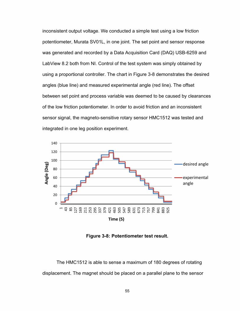
inconsistent output voltage. We conducted a simple test using a low friction

potentiometer, Murata SV01L, in one joint. The set point and sensor response

was generated and recorded by a Data Acquisition Card (DAQ) USB-6259 and

LabView 8.2 both from NI. Control of the test system was simply obtained by

using a proportional controller. The chart in Figure 3-8 demonstrates the desired

angles (blue line) and measured experimental angle (red line). The offset

between set point and process variable was deemed to be caused by clearances

of the low friction potentiometer. In order to avoid friction and an inconsistent

sensor signal, the magneto-sensitive rotary sensor HMC1512 was tested and

integrated in one leg position experiment.

0

20

40

60

80

100

120

140

1 43 85 127

169

211

253

295

337

379

421

463

505

547

589

631

673

715

757

799

841

883

925

Angle (D

eg)

Time (S)

desired angle

experimental angle

Figure 3-8: Potentiometer test result.

The HMC1512 is able to sense a maximum of 180 degrees of rotating

displacement. The magnet should be placed on a parallel plane to the sensor

55

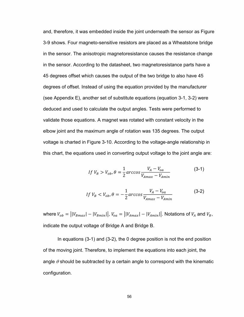
and, therefore, it was embedded inside the joint underneath the sensor as Figure

3-9 shows. Four magneto-sensitive resistors are placed as a Wheatstone bridge

in the sensor. The anisotropic magnetoresistance causes the resistance change

in the sensor. According to the datasheet, two magnetoresistance parts have a

45 degrees offset which causes the output of the two bridge to also have 45

degrees of offset. Instead of using the equation provided by the manufacturer

(see Appendix E), another set of substitute equations (equation 3-1, 3-2) were

deduced and used to calculate the output angles. Tests were performed to

validate those equations. A magnet was rotated with constant velocity in the

elbow joint and the maximum angle of rotation was 135 degrees. The output

voltage is charted in Figure 3-10. According to the voltage-angle relationship in

this chart, the equations used in converting output voltage to the joint angle are:

,12 (3-1)

,12 (3-2)

where | | | | , | | | | . Notations of and ,

indicate the output voltage of Bridge A and Bridge B.

In equations (3-1) and (3-2), the 0 degree position is not the end position

of the moving joint. Therefore, to implement the equations into each joint, the

angle θ should be subtracted by a certain angle to correspond with the kinematic

configuration.

56

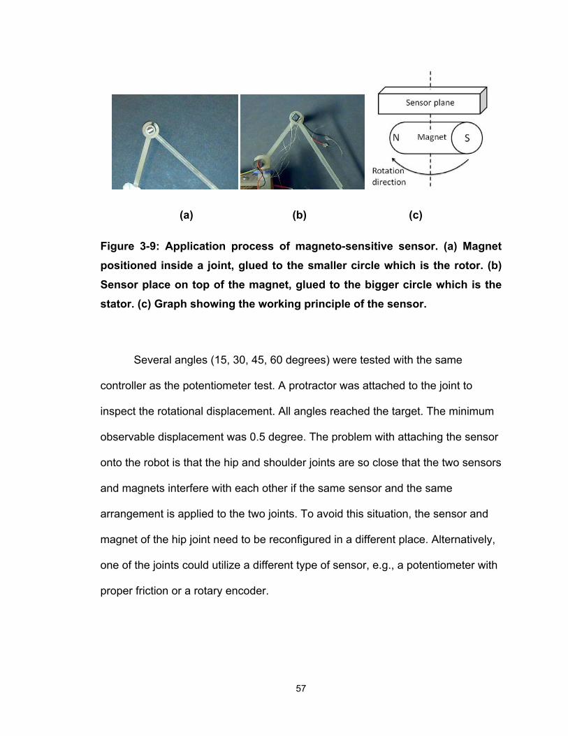
(a) (b) (c)

Figure 3-9: Application process of magneto-sensitive sensor. (a) Magnet positioned inside a joint, glued to the smaller circle which is the rotor. (b) Sensor place on top of the magnet, glued to the bigger circle which is the stator. (c) Graph showing the working principle of the sensor.

Several angles (15, 30, 45, 60 degrees) were tested with the same

controller as the potentiometer test. A protractor was attached to the joint to

inspect the rotational displacement. All angles reached the target. The minimum

observable displacement was 0.5 degree. The problem with attaching the sensor

onto the robot is that the hip and shoulder joints are so close that the two sensors

and magnets interfere with each other if the same sensor and the same

arrangement is applied to the two joints. To avoid this situation, the sensor and

magnet of the hip joint need to be reconfigured in a different place. Alternatively,

one of the joints could utilize a different type of sensor, e.g., a potentiometer with

proper friction or a rotary encoder.

57

‐80

‐60

‐40

‐20

0

20

40

60

80

1 13 25 37 49 61 73 85 97 109

121

133

145

157

169

181

193

205

217

229

241

253

Outpu

t Voltage (m

V)

Time (S)

Bridge A

Bridge B

Figure 3-10: Magneto-sensitive sensor test result. The magnet was rotating 135 degrees with constant velocity.

Compared to the potentiometer, four lines of signal output from each

sensor complicate the wiring and displacement calculation. Though the four lines

could be differentiated before connecting to the processor, each sensor will have

two signals, which results in a total of 36 wires from the sensors to the processor

for the entire robot. The two signals need to be calculated with the set of

equations to convert into angular position. For these reasons, and despite the

difficulties encountered while trying to embed all joints with the HMC1512 rotary

sensor, implements the magneto-sensitive sensor into the robot is a feasible

solution.

58

59

3.3.4 Controller design and other electronics

A PID controller was built in LabVIEW after we decided on the final

actuators and sensors (Figure 3-11). The DAQ USB-6259 receives and transfers

signals between the hardware, which are the sensor and motor, and the PC,

where the controller, implemented in LabVIEW, is running. In each joint, the DAQ

sends a one-line PWM signal to the converter with a set duty cycle and

frequency. Afterwards, the converter outputs two lines of signals to the H-bridge,

one of them is the same as the original PWM and the other is reversed. The H-

bridge links the two poles of the motor, driving it to rotate with desired speed and

direction.

The sensor outputs four signals from two bridges, which are differentiated

in the DAQ to provide two output signals to the controller. The two signals are

converted into angular position with the equations (3-1) and (3-2) in the LabVIEW

controller. The DAQ is connected to the PC by a USB port. The scheme of the

control loop is shown in Figure 3-12. Validation is given in a test of one leg

position control, which is going to be described in Chapter 4. Unfortunately,

current DAQ manufactured by NI could only generate PWM in maximum of eight

individual digital channels. Prototype 2, however, requires 18 signals for

controlling all the motors. If LabVIEW and the DAQ are used to control the entire

system, additional electronics, such as a multiplexer and Field-Programmable

Gate Array (FPGA), should be added in a proper circuit to arrange the high

number of input and output wires.

Figure 3-11: Block diagram of controller design in LabVIEW 8.2.

60

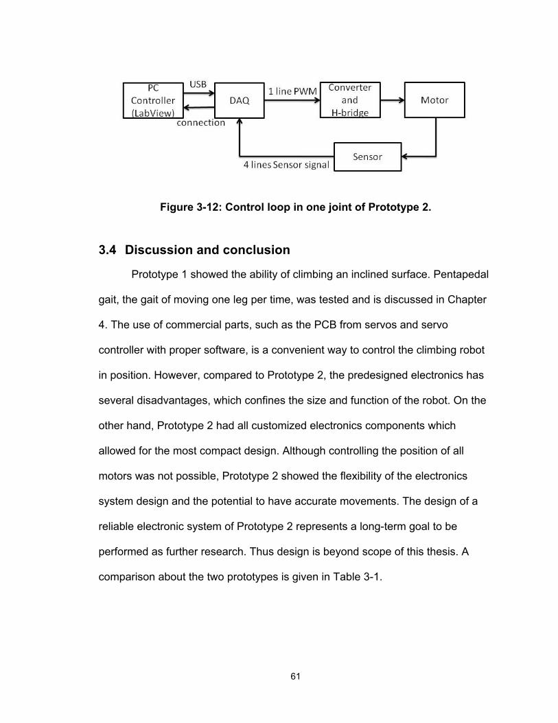
Figure 3-12: Control loop in one joint of Prototype 2.

3.4 Discussion and conclusion

Prototype 1 showed the ability of climbing an inclined surface. Pentapedal

gait, the gait of moving one leg per time, was tested and is discussed in Chapter

4. The use of commercial parts, such as the PCB from servos and servo

controller with proper software, is a convenient way to control the climbing robot

in position. However, compared to Prototype 2, the predesigned electronics has

several disadvantages, which confines the size and function of the robot. On the

other hand, Prototype 2 had all customized electronics components which

allowed for the most compact design. Although controlling the position of all

motors was not possible, Prototype 2 showed the flexibility of the electronics

system design and the potential to have accurate movements. The design of a

reliable electronic system of Prototype 2 represents a long-term goal to be

performed as further research. Thus design is beyond scope of this thesis. A

comparison about the two prototypes is given in Table 3-1.

61

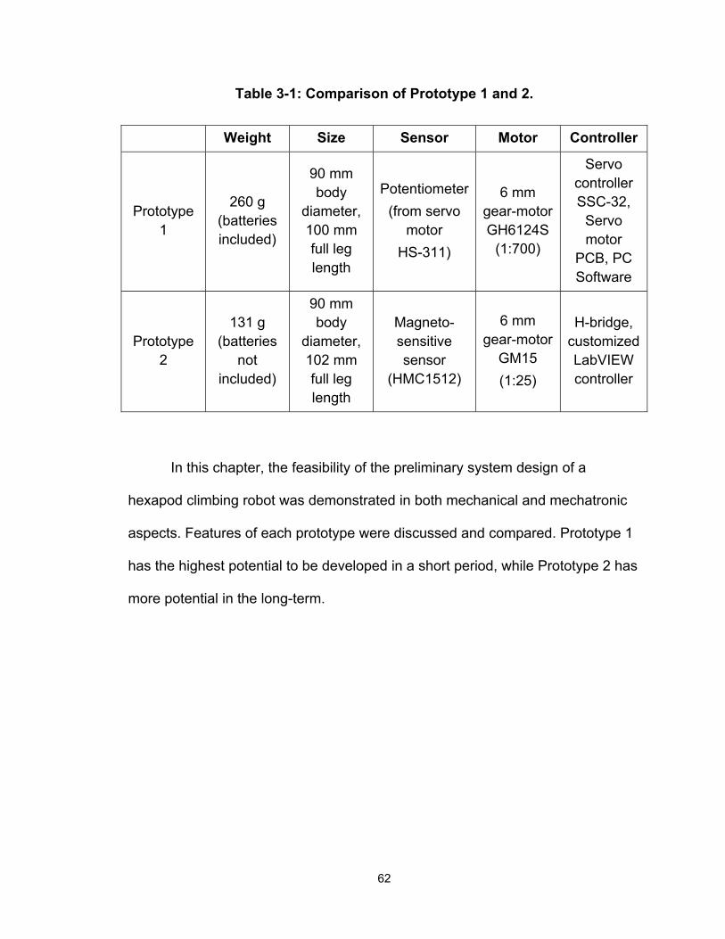
Table 3-1: Comparison of Prototype 1 and 2.

Weight Size Sensor Motor Controller

Prototype 1

260 g (batteries included)

90 mm body

diameter, 100 mm full leg length

Potentiometer(from servo

motor HS-311)

6 mm gear-motor GH6124S

(1:700)

Servo controller SSC-32,

Servo motor

PCB, PC Software

Prototype 2

131 g (batteries

not included)

90 mm body

diameter, 102 mm full leg length

Magneto-sensitive sensor

(HMC1512)

6 mm gear-motor

GM15 (1:25)

H-bridge, customized LabVIEW controller

In this chapter, the feasibility of the preliminary system design of a

hexapod climbing robot was demonstrated in both mechanical and mechatronic

aspects. Features of each prototype were discussed and compared. Prototype 1

has the highest potential to be developed in a short period, while Prototype 2 has

more potential in the long-term.

62

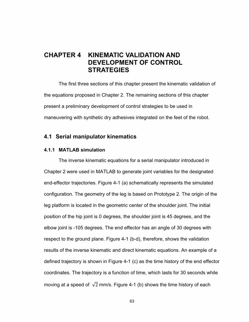
CHAPTER 4 KINEMATIC VALIDATION AND DEVELOPMENT OF CONTROL STRATEGIES

The first three sections of this chapter present the kinematic validation of

the equations proposed in Chapter 2. The remaining sections of this chapter

present a preliminary development of control strategies to be used in

maneuvering with synthetic dry adhesives integrated on the feet of the robot.

4.1 Serial manipulator kinematics

63

4.1.1 MATLAB simulation

The inverse kinematic equations for a serial manipulator introduced in

Chapter 2 were used in MATLAB to generate joint variables for the designated

end-effector trajectories. Figure 4-1 (a) schematically represents the simulated

configuration. The geometry of the leg is based on Prototype 2. The origin of the

leg platform is located in the geometric center of the shoulder joint. The initial

position of the hip joint is 0 degrees, the shoulder joint is 45 degrees, and the

elbow joint is -105 degrees. The end effector has an angle of 30 degrees with

respect to the ground plane. Figure 4-1 (b-d), therefore, shows the validation

results of the inverse kinematic and direct kinematic equations. An example of a

defined trajectory is shown in Figure 4-1 (c) as the time history of the end effector

coordinates. The trajectory is a function of time, which lasts for 30 seconds while

moving at a speed of √2 mm/s. Figure 4-1 (b) shows the time history of each

joint while the end effector was moving as Figure 4-1 (c) defines; joint rotation

angles were generated by utilizing inverse kinematic equations (2-11) - (2-14).

Figure 4-1 (d) shows the time history of the end effector coordinates generated

by direct kinematic equation (2) – (5) using the result of the joint variables

generated in the inverse kinematics shown in Figure 4-1 (b). Figure (c) and (d)

are identical, which means the direct kinematic and inverse kinematic equations

are consistent with each other, proving the equations are correct and ready for

application.

For a fixed end-effector position, only one set of joint variables achieves

the goal in a continuous trajectory. In other words, the orientation of the end

effector in a designated position is fixed, which means that, if we need to control

the end tip of the leg in both position and orientation, the current design will not

be sufficient. As the direction of the leg tip does not really matter while it is in the

swing phase, the main concern of the leg tip direction is the approaching and

detaching angle for controlling the properties of the synthetic dry adhesion.

Another degree of freedom, or an extra joint, needs to be added for controlling

the feet direction.

In the most recent foot design, the extra joint was designed to be passive

and was fabricated using Polydimethylsiloxane (PDMS) as an ankle (Figure 4-2

(a)). As the material is soft, it allows the end tip of the leg to have three more

degrees of freedom, allowing for rotation in all directions when the feet are

attached to a surface. The three extra passive DOFs are modeled as a spherical

joint in Chapter 2. Another potential design of the passive joint is the dual layer

64

65

foot (Figure 4-2 (b)), which may be used in future designs. The dual layers

include the upper layer, which consists of spaced macro pillars attached to a

one-piece PDMS foot, and the lower layer, which is fabricated out of micro

adhesive pads attached to each pillar of the upper layer. This design is more

compliant to the contacting surface due to its multi-scale structure.

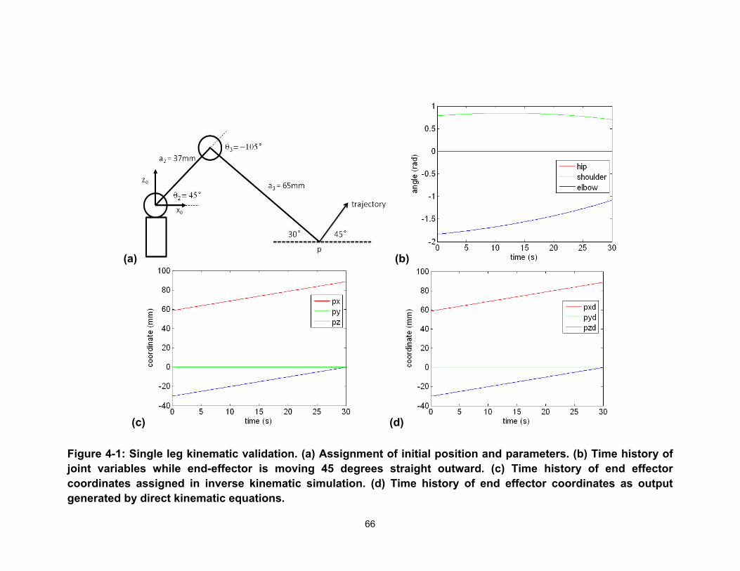
(a) (b)

(c) (d)

Figure 4-1: Single leg kinematic validation. (a) Assignment of initial position and parameters. (b) Time history of joint variables while end-effector is moving 45 degrees straight outward. (c) Time history of end effector coordinates assigned in inverse kinematic simulation. (d) Time history of end effector coordinates as output generated by direct kinematic equations.

66

(a) (b)

Figure 4-2: Ankle on a foot fabricated using PDMS (a) and a dual-layer foot (b).

4.1.2 Position control test based on Prototype 2

In order to test the PID controller designed in LabVIEW and to validate the

one leg open chain kinematics, a position control test based on Prototype 2 was

performed with the setup as shown in Figure 4-3. Wires at the back were linked

to the DAQ PCI-6071E. The motor signals were provided by the digital ports in

PWM and the sensor signals were feedback into DAQ’s analog channels. As

Chapter 3 described, PID control is provided by LabVIEW. A MATLAB script was

written in a node in the controller. By using MATLAB results, three motors were

given the data and the end-effector was monitored to verify if it achieved the

expected trajectory, which was a 45 degree straight line outward. To avoid

overshoot, the joints were moved in very small steps at a relatively slow speed

(√2 mm/s). Measuring with a protractor, the end effector was observed to follow

the predefined trajectory.

Test results of the control loop are shown in Figure 4-4. The set point

denotes the data generated by MATLAB simulation and sensor 2 and sensor 3

denote the sensor feedback signals in the shoulder and elbow joints,

67

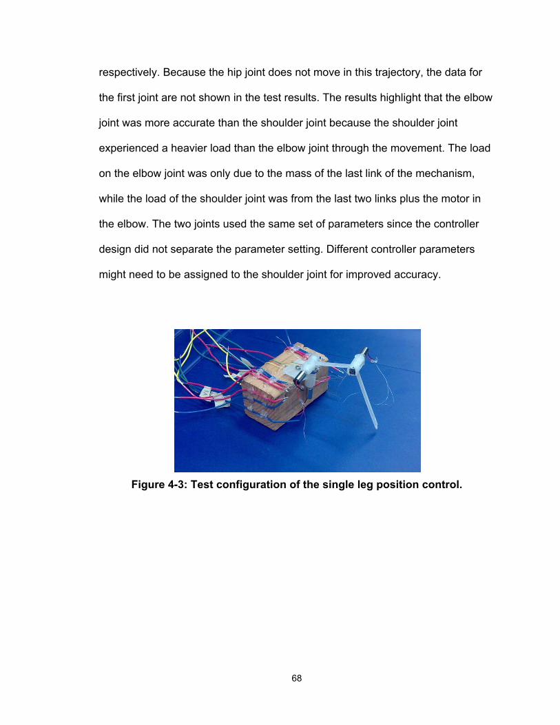
respectively. Because the hip joint does not move in this trajectory, the data for

the first joint are not shown in the test results. The results highlight that the elbow

joint was more accurate than the shoulder joint because the shoulder joint

experienced a heavier load than the elbow joint through the movement. The load

on the elbow joint was only due to the mass of the last link of the mechanism,

while the load of the shoulder joint was from the last two links plus the motor in

the elbow. The two joints used the same set of parameters since the controller

design did not separate the parameter setting. Different controller parameters

might need to be assigned to the shoulder joint for improved accuracy.

Figure 4-3: Test configuration of the single leg position control.

68

0.6

0.65

0.7

0.75

0.8

0.85

0.9

1 3 5 7 9 11 13 15 17 19 21 23 25 27 29

joint a

ngle (rad

ian)

Time (s)

Shoulder joint

set point 2

sensor 2

‐1.9

‐1.8

‐1.7

‐1.6

‐1.5

‐1.4

‐1.3

‐1.2

‐1.1

‐1

1 3 5 7 9 11 13 15 17 19 21 23 25 27 29

joint a

ngle (rad

ian)

Time (s)

Elbow joint

set point 3

sensor 3

Figure 4-4: Controller test result of the shoulder joint (sensor 2) and elbow joint (sensor 3).

69

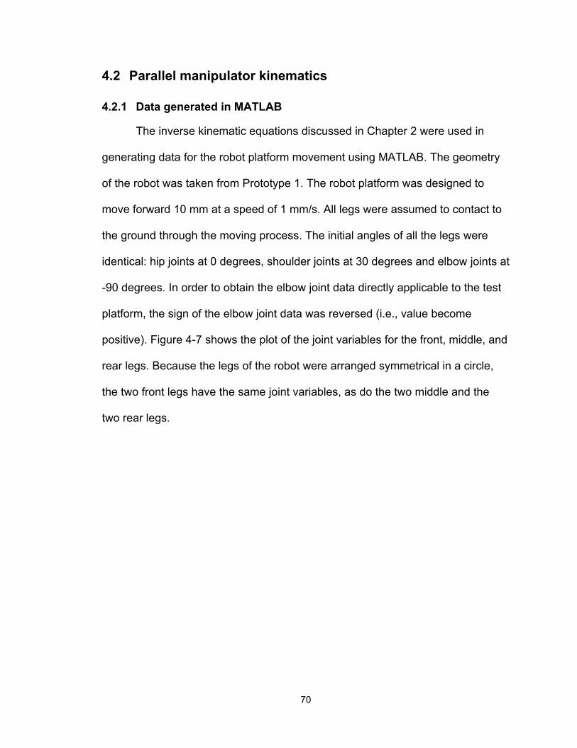
4.2 Parallel manipulator kinematics

4.2.1 Data generated in MATLAB

The inverse kinematic equations discussed in Chapter 2 were used in

generating data for the robot platform movement using MATLAB. The geometry

of the robot was taken from Prototype 1. The robot platform was designed to

move forward 10 mm at a speed of 1 mm/s. All legs were assumed to contact to

the ground through the moving process. The initial angles of all the legs were

identical: hip joints at 0 degrees, shoulder joints at 30 degrees and elbow joints at

-90 degrees. In order to obtain the elbow joint data directly applicable to the test

platform, the sign of the elbow joint data was reversed (i.e., value become

positive). Figure 4-7 shows the plot of the joint variables for the front, middle, and

rear legs. Because the legs of the robot were arranged symmetrical in a circle,

the two front legs have the same joint variables, as do the two middle and the

two rear legs.

70

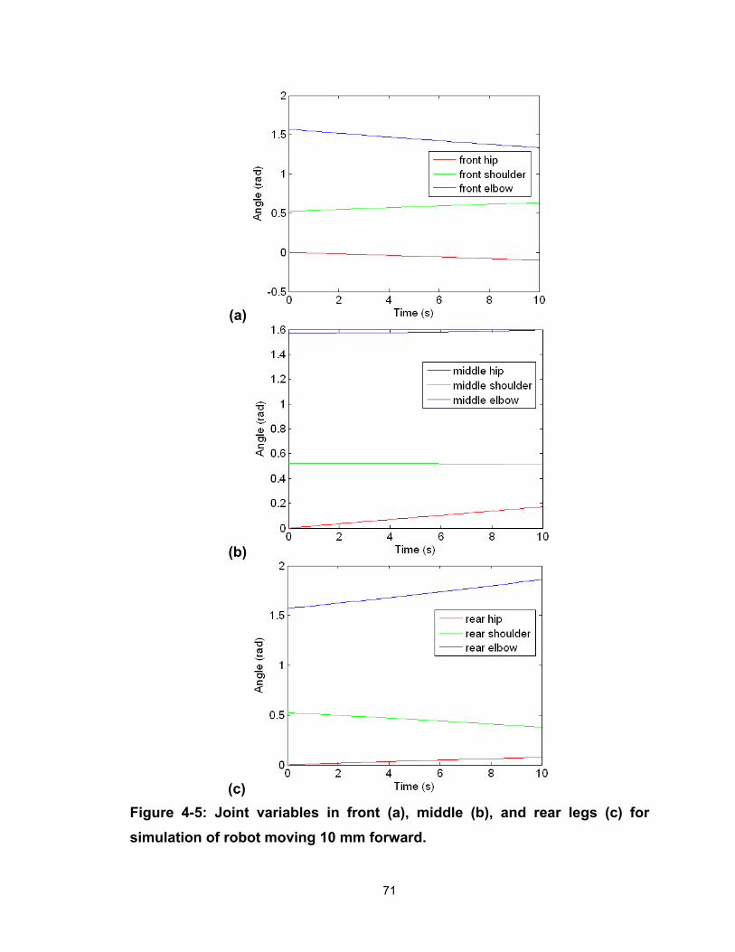
(a)

(b)

(c) Figure 4-5: Joint variables in front (a), middle (b), and rear legs (c) for simulation of robot moving 10 mm forward.

71

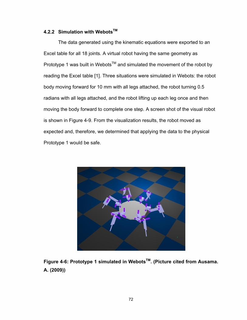
4.2.2 Simulation with WebotsTM

The data generated using the kinematic equations were exported to an

Excel table for all 18 joints. A virtual robot having the same geometry as

Prototype 1 was built in WebotsTM and simulated the movement of the robot by

reading the Excel table [1]. Three situations were simulated in Webots: the robot

body moving forward for 10 mm with all legs attached, the robot turning 0.5

radians with all legs attached, and the robot lifting up each leg once and then

moving the body forward to complete one step. A screen shot of the visual robot

is shown in Figure 4-9. From the visualization results, the robot moved as

expected and, therefore, we determined that applying the data to the physical

Prototype 1 would be safe.

Figure 4-6: Prototype 1 simulated in WebotsTM. (Picture cited from Ausama. A. (2009))

72

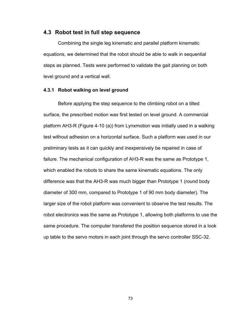
4.3 Robot test in full step sequence

Combining the single leg kinematic and parallel platform kinematic

equations, we determined that the robot should be able to walk in sequential

steps as planned. Tests were performed to validate the gait planning on both

level ground and a vertical wall.

4.3.1 Robot walking on level ground

Before applying the step sequence to the climbing robot on a tilted

surface, the prescribed motion was first tested on level ground. A commercial

platform AH3-R (Figure 4-10 (a)) from Lynxmotion was initially used in a walking

test without adhesion on a horizontal surface. Such a platform was used in our

preliminary tests as it can quickly and inexpensively be repaired in case of

failure. The mechanical configuration of AH3-R was the same as Prototype 1,

which enabled the robots to share the same kinematic equations. The only

difference was that the AH3-R was much bigger than Prototype 1 (round body

diameter of 300 mm, compared to Prototype 1 of 90 mm body diameter). The

larger size of the robot platform was convenient to observe the test results. The

robot electronics was the same as Prototype 1, allowing both platforms to use the

same procedure. The computer transfered the position sequence stored in a look

up table to the servo motors in each joint through the servo controller SSC-32.

73

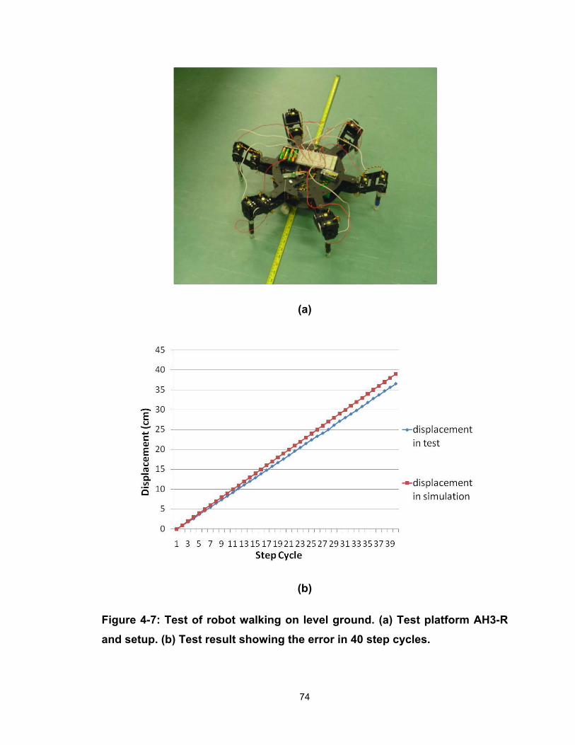
(a)

(b)

Figure 4-7: Test of robot walking on level ground. (a) Test platform AH3-R and setup. (b) Test result showing the error in 40 step cycles.

74

The motion of the robotic legs was designed to move the robot 10 mm

forward for each step in a pentapedal gait, which moved one leg at a time. Each

step was planned as follows: beginning with the Left Front Leg (LFL) and

proceeding in counter clockwise, each leg was lifted, moved, and lowered one at

a time, followed by the forward motion of the robot body. The tip of the leg was

detached following a 45-degree trajectory to minimize the robot’s power

consumption (a detailed discussion is presented in the next section). The legs

attached to the ground at 10 mm forward from the initial position. The initial and

end positions with respect to the joint variables were identical in order to form a

repeatable step cycle. The initial angles of the leg had the shoulder joint at 30

degrees, the elbow joint at -120 degrees, and the hip joint at 0 degrees (Figure 4-

7 (a)), which poses the tibia perpendicular to the ground. Different initial positions

were also tested, but the motors of the AH3-R have limited torque and this

prevents exploring a wide range of feasible trajectories. For instance, with the

tibia forming certain angles to the ground, e.g. 60 degrees, the robot body

collapses due to gravity acting on the body weight. With a perpendicular tibia to

the ground, however, this problem is avoided.

With the above configuration, the robot was set to walk in the same gait

repeatedly for 40 step cycles. Test results are shown in Figure 4-7 (b). The robot

was supposed to have a final displacement of 400 mm (40 cm), but it only

reached 36.5 cm due to a 1 mm error in almost every step. The error was

probably due to the mechanical clearances of the 18 revolute joints of the robot.

However, the test still validated the kinematic equations and the planned gait.

75

4.3.2 Robot climbing on a vertical wall

Prototype 1 was tested on a tilted surface with pentapedal gait and,

eventually, on a vertical Plexiglas surface (Figure 4-9). The tip of the leg was

attached to a piece of single-layer adhesive through a silicone interface. This

silicone interface formed the ankle mechanism (Figure 4-8) instead of the PDMS

ankle mentioned in section 4.1.1. Different postures were tested for vertical

climbing, including the one tested on the horizontal ground. The clearance of

each joint caused the robot’s body to drop a few millimeters in the direction of

gravity. To minimize the gravitational effects on the robot’s movement, the center

of mass (COM), which is located at the geometric center of the robot body, was

placed as close to the wall as possible. The middle legs were positioned upward,

close to the front legs, because the robot tends to fall off the wall when the front

legs detach first. By taking into account the results obtained during the force

distribution tests (Appendix A), the middle legs, which were positioned closer to

the front legs, were used to reinforce the front legs’ adhesion.

The initial position of the legs when the robot climbs on a vertical wall

were as follows: the shoulder joints were at 20 degrees, the elbow joints were at -

50 degrees, and the hip joints were at 0 degrees for the front and rear legs and ±

45 degrees for the middle legs.

The gait was slightly different than previous conditions: first, the body was

moved upward by 5 mm (Figure 4-9 (a-b)), then each leg was moved upwards by

5 mm from the LFL to LML in CCW sequence to form the full step cycle (Figure

4-9 (c-d)). Before starting the step, each foot was preloaded manually. From

76

77

observation, the displacement error should be bigger than the level ground test.

The robot was not able to finish the second step cycle due to insufficient

preloading on the adhesive to hold the robot in position for the next step cycle.

Figure 4-8: Foot used in the vertical climbing experiment. Single layer adhesive was glued to the leg tip with silicone sealant.

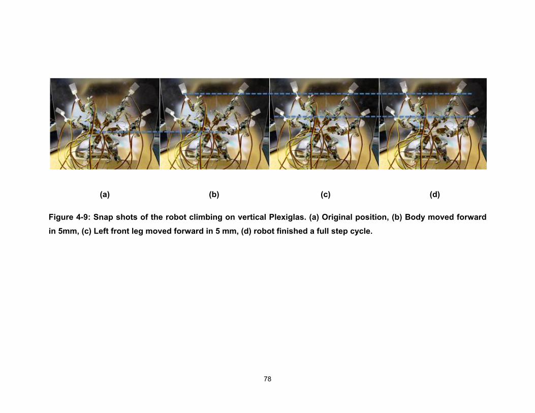
(a) (b) (c) (d)

Figure 4-9: Snap shots of the robot climbing on vertical Plexiglas. (a) Original position, (b) Body moved forward in 5mm, (c) Left front leg moved forward in 5 mm, (d) robot finished a full step cycle.

78

4.4 Trajectory selection for releasing the dry adhesive

The trajectory of the tip of each leg was at 45 degrees with respect to the

surface for all the tests presented in the previous section. In this section, the

motivation for selecting this particular trajectory is provided.

4.4.1 Theory of peeling an elastic thin film

The robot’s foot was fabricated with thin layer of PDMS using the most

recent adhesive design. The design is considered as an elastic thin film with dry

adhesion attached at the bottom. As mentioned in Chapter 1, dry adhesives are

easier to release when they are peeled from the surface. Several studies have

investigated the efficiency of peeling elastic thin films and micro-fibrila, such as

the gecko seta, in a certain direction [16-18][30-33]. Kendall [35] proposed a

theory of peeling elastic thin films from a rigid substrate that indicated the

relationship between peeling force and peeling angle (Figure 4-10:

1

2 1 0 (4-1)

where b, d, and E denote the width, thickness, and Young’s modulus of the

elastic thin film. θ denotes the peeling angle between thin film and substrate. F

represents the peeling force in the same angle θ with respect to the substrate. R

denotes the adhesive energy, which is the experimental energy required to

fracture a unit area of the interface. In equation (4-1), the first term is called the

elastic term, the second is called the potential term, and the last term represents

the surface term. Usually the elastic term may be neglected unless the material is

79

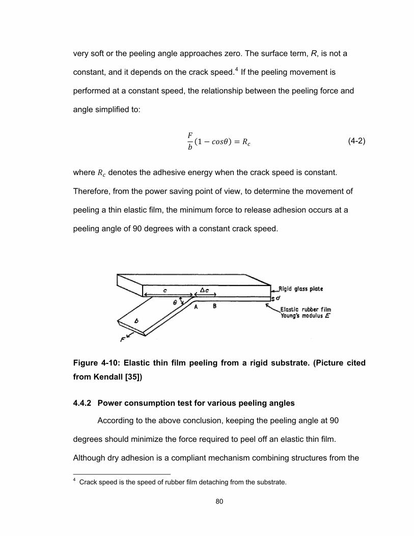
very soft or the peeling angle approaches zero. The surface term, R, is not a

constant, and it depends on the crack speed.4 If the peeling movement is

performed at a constant speed, the relationship between the peeling force and

angle simplified to:

1 (4-2)

where denotes the adhesive energy when the crack speed is constant.

Therefore, from the power saving point of view, to determine the movement of

peeling a thin elastic film, the minimum force to release adhesion occurs at a

peeling angle of 90 degrees with a constant crack speed.

Figure 4-10: Elastic thin film peeling from a rigid substrate. (Picture cited from Kendall [35])

4.4.2 Power consumption test for various peeling angles

According to the above conclusion, keeping the peeling angle at 90

degrees should minimize the force required to peel off an elastic thin film.

Although dry adhesion is a compliant mechanism combining structures from the

4 Crack speed is the speed of rubber film detaching from the substrate.

80

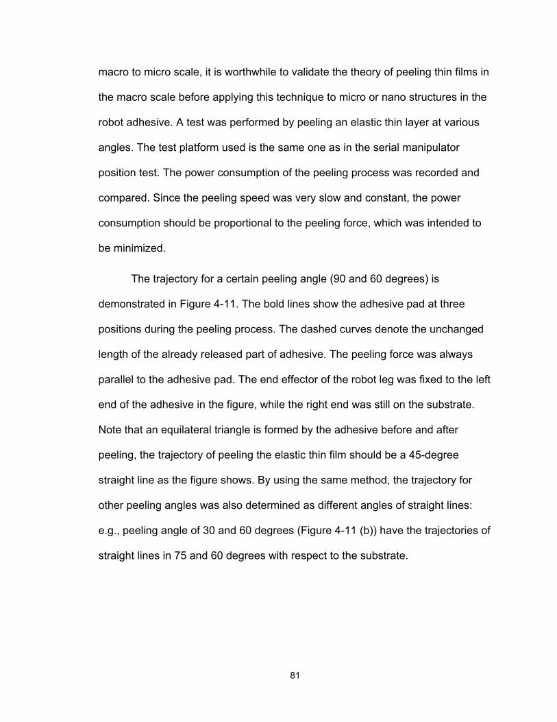
macro to micro scale, it is worthwhile to validate the theory of peeling thin films in

the macro scale before applying this technique to micro or nano structures in the

robot adhesive. A test was performed by peeling an elastic thin layer at various

angles. The test platform used is the same one as in the serial manipulator

position test. The power consumption of the peeling process was recorded and

compared. Since the peeling speed was very slow and constant, the power

consumption should be proportional to the peeling force, which was intended to

be minimized.

The trajectory for a certain peeling angle (90 and 60 degrees) is

demonstrated in Figure 4-11. The bold lines show the adhesive pad at three

positions during the peeling process. The dashed curves denote the unchanged

length of the already released part of adhesive. The peeling force was always

parallel to the adhesive pad. The end effector of the robot leg was fixed to the left

end of the adhesive in the figure, while the right end was still on the substrate.

Note that an equilateral triangle is formed by the adhesive before and after

peeling, the trajectory of peeling the elastic thin film should be a 45-degree

straight line as the figure shows. By using the same method, the trajectory for

other peeling angles was also determined as different angles of straight lines:

e.g., peeling angle of 30 and 60 degrees (Figure 4-11 (b)) have the trajectories of

straight lines in 75 and 60 degrees with respect to the substrate.

81

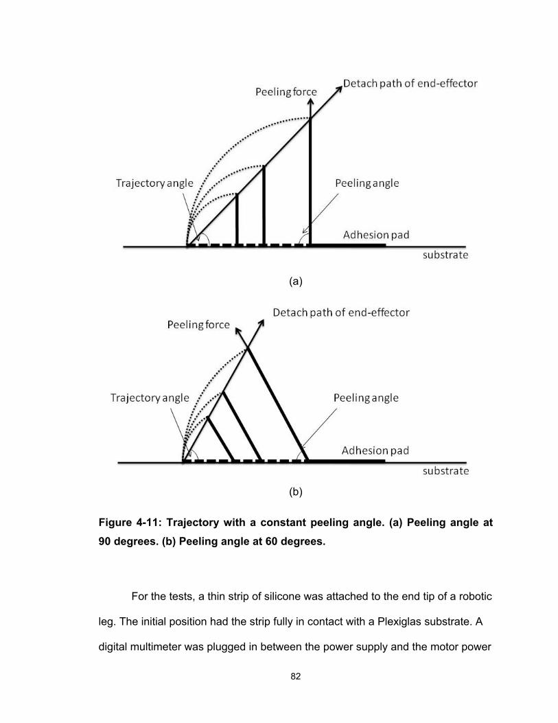
(a)

(b)

Figure 4-11: Trajectory with a constant peeling angle. (a) Peeling angle at 90 degrees. (b) Peeling angle at 60 degrees.

For the tests, a thin strip of silicone was attached to the end tip of a robotic

leg. The initial position had the strip fully in contact with a Plexiglas substrate. A

digital multimeter was plugged in between the power supply and the motor power

82

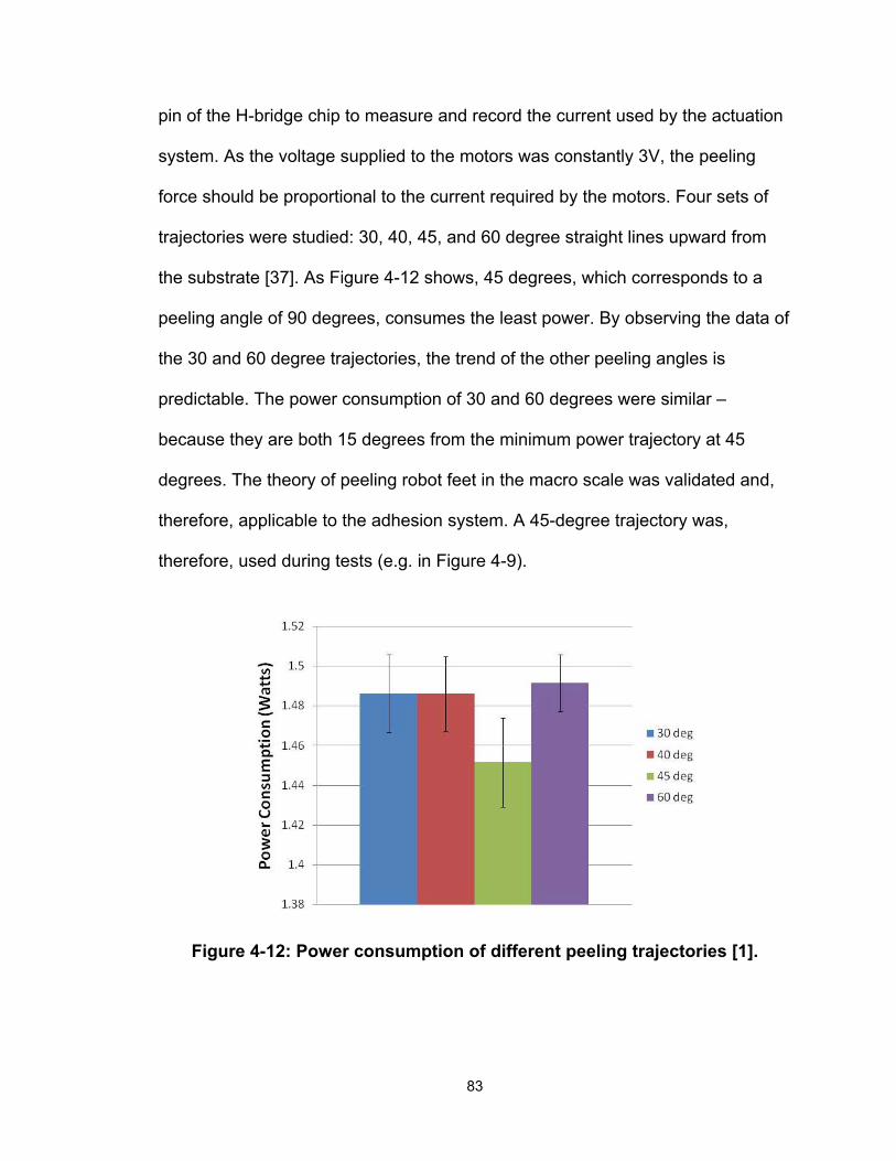
pin of the H-bridge chip to measure and record the current used by the actuation

system. As the voltage supplied to the motors was constantly 3V, the peeling

force should be proportional to the current required by the motors. Four sets of

trajectories were studied: 30, 40, 45, and 60 degree straight lines upward from

the substrate [37]. As Figure 4-12 shows, 45 degrees, which corresponds to a

peeling angle of 90 degrees, consumes the least power. By observing the data of

the 30 and 60 degree trajectories, the trend of the other peeling angles is

predictable. The power consumption of 30 and 60 degrees were similar –

because they are both 15 degrees from the minimum power trajectory at 45

degrees. The theory of peeling robot feet in the macro scale was validated and,

therefore, applicable to the adhesion system. A 45-degree trajectory was,

therefore, used during tests (e.g. in Figure 4-9).

Figure 4-12: Power consumption of different peeling trajectories [1].

83

4.5 Optimizing the adhesive force

Different tests based on Prototype 2 were performed to investigate the

optimal position that fully utilizes the unique properties of dry adhesion.

4.5.1 Optimal leg angle for maximizing the adhesive force

In order to determine the most power efficient joint torques for reliable

adhesion, experiments were performed by measuring power consumption while

the robot was attached to a wall. A simple test was initially performed to identify

the optimal angle that the legs should assume to maximize the adhesive force.

Tests were completed with a prototype having embedded PDMS feet. Each time

after a measurement, the PDMS feet were cleaned by Scotch® tape to remove

dust and allow them to have the same adhesion property, thus enabling

repeatable measurements. A simple robot having three symmetric legs, each one

controlled by a single motor, was used for this experiment. The tripod, and the

angle α which was investigated in this preliminary analysis, are shown in Figure

4-13.

84

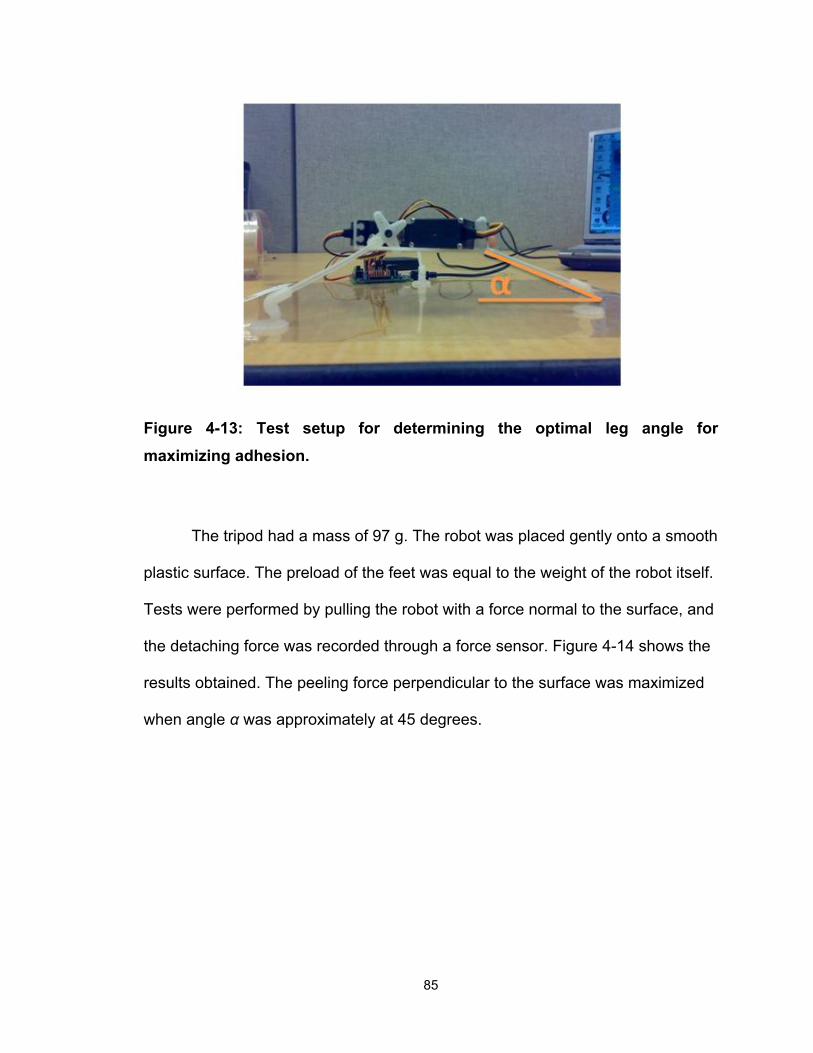
Figure 4-13: Test setup for determining the optimal leg angle for maximizing adhesion.

The tripod had a mass of 97 g. The robot was placed gently onto a smooth

plastic surface. The preload of the feet was equal to the weight of the robot itself.

Tests were performed by pulling the robot with a force normal to the surface, and

the detaching force was recorded through a force sensor. Figure 4-14 shows the

results obtained. The peeling force perpendicular to the surface was maximized

when angle α was approximately at 45 degrees.

85

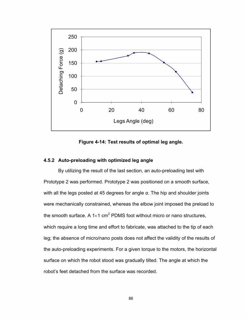
0

50

100

150

200

250

0 20 40 60 8

Det

achi

ng F

orce

(g)

Legs Angle (deg)

0

Figure 4-14: Test results of optimal leg angle.

4.5.2 Auto-preloading with optimized leg angle

By utilizing the result of the last section, an auto-preloading test with

Prototype 2 was performed. Prototype 2 was positioned on a smooth surface,

with all the legs posted at 45 degrees for angle α. The hip and shoulder joints

were mechanically constrained, whereas the elbow joint imposed the preload to

the smooth surface. A 1×1 cm2 PDMS foot without micro or nano structures,

which require a long time and effort to fabricate, was attached to the tip of each

leg; the absence of micro/nano posts does not affect the validity of the results of

the auto-preloading experiments. For a given torque to the motors, the horizontal

surface on which the robot stood was gradually tilted. The angle at which the

robot’s feet detached from the surface was recorded.

86

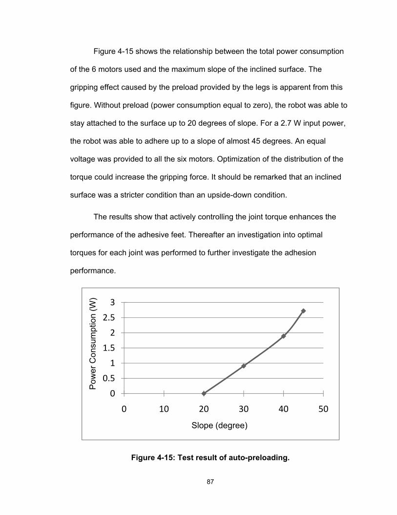
Figure 4-15 shows the relationship between the total power consumption

of the 6 motors used and the maximum slope of the inclined surface. The

gripping effect caused by the preload provided by the legs is apparent from this

figure. Without preload (power consumption equal to zero), the robot was able to

stay attached to the surface up to 20 degrees of slope. For a 2.7 W input power,

the robot was able to adhere up to a slope of almost 45 degrees. An equal

voltage was provided to all the six motors. Optimization of the distribution of the

torque could increase the gripping force. It should be remarked that an inclined

surface was a stricter condition than an upside-down condition.

The results show that actively controlling the joint torque enhances the

performance of the adhesive feet. Thereafter an investigation into optimal

torques for each joint was performed to further investigate the adhesion

performance.

0

0.5

1

1.5

2

2.5

3

0 10 20 30 40 5

Pow

er C

onsu

mpt

ion

(W)

Slope (degree)

0

Figure 4-15: Test result of auto-preloading.

87

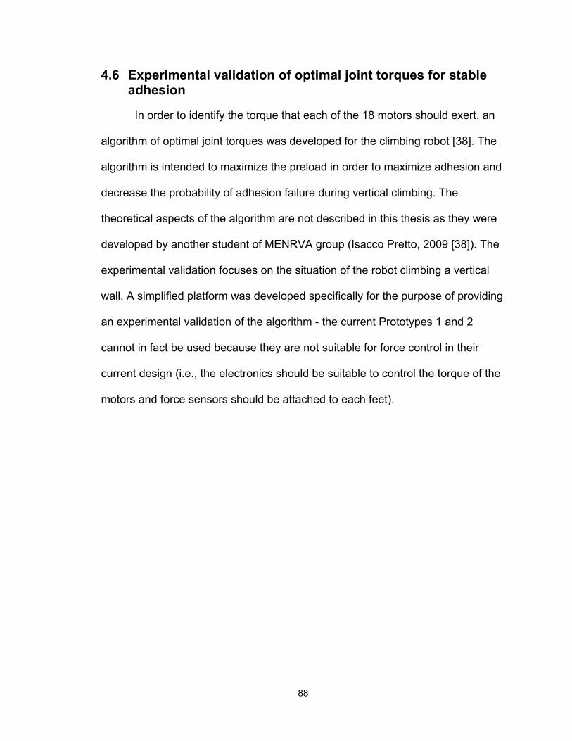
4.6 Experimental validation of optimal joint torques for stable adhesion

In order to identify the torque that each of the 18 motors should exert, an

algorithm of optimal joint torques was developed for the climbing robot [38]. The

algorithm is intended to maximize the preload in order to maximize adhesion and

decrease the probability of adhesion failure during vertical climbing. The

theoretical aspects of the algorithm are not described in this thesis as they were

developed by another student of MENRVA group (Isacco Pretto, 2009 [38]). The

experimental validation focuses on the situation of the robot climbing a vertical

wall. A simplified platform was developed specifically for the purpose of providing

an experimental validation of the algorithm - the current Prototypes 1 and 2

cannot in fact be used because they are not suitable for force control in their

current design (i.e., the electronics should be suitable to control the torque of the

motors and force sensors should be attached to each feet).

88

Figure 4-16: CAD model of simplified robot.

4.6.1 Experimental setup

The simplified platform includes two parts: the robot and the contact point

sensing mechanism. The robot has three legs with equal length (Figure 4-16).

The motors are arranged in a line with the motor shafts 50 mm apart. The leg

length is also 50 mm. At the end of each leg, a revolute joint was designed to

connect the sensor with a proper interface. Each sensor was fixed to a flat plate

which was aligned and glued to a vertical surface. Because each contacting point

was fixed to the wall, the robot was over constrained and could not move even

when the motors were activated. The test platform with both parts assembled is

shown in Figure 4-17.

89

(a) (b)

Figure 4-17: Assembled test platform. (a) Front view. (b) Side view with coordinates used in the algorithm.

The motors (Maxon RE25) were able to provide relatively stable torques

with a fixed current input. The maximum stall torque was 240 mNm according to

the datasheet. Each motor was connected to a separate channel of the power

supplies. The three sensors, from the bottom up, are a 6-axis Force/Torque

sensor Gamma from ATI Industrial Automation, load cells LSM 300 and LCM 300

from Futek. A controller also from ATI was connected to the Gamma and a demo

program was used to monitor the contacting force of the lower joint. For the load

cells, a customized amplifier with a gain of 430 was used in to output the force

reading of the upper two joints. A digital multimeter was connected to the

90

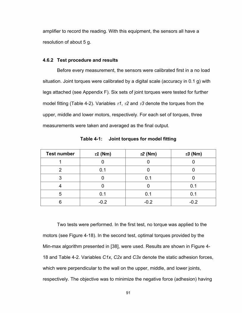
amplifier to record the reading. With this equipment, the sensors all have a

resolution of about 5 g.

4.6.2 Test procedure and results

Before every measurement, the sensors were calibrated first in a no load

situation. Joint torques were calibrated by a digital scale (accuracy in 0.1 g) with

legs attached (see Appendix F). Six sets of joint torques were tested for further

model fitting (Table 4-2). Variables τ1, τ2 and τ3 denote the torques from the

upper, middle and lower motors, respectively. For each set of torques, three

measurements were taken and averaged as the final output.

Table 4-1: Joint torques for model fitting

Test number τ1 (Nm) τ2 (Nm) τ3 (Nm) 1 0 0 0

2 0.1 0 0

3 0 0.1 0

4 0 0 0.1

5 0.1 0.1 0.1

6 -0.2 -0.2 -0.2

Two tests were performed. In the first test, no torque was applied to the

motors (see Figure 4-18). In the second test, optimal torques provided by the

Min-max algorithm presented in [38], were used. Results are shown in Figure 4-

18 and Table 4-2. Variables C1x, C2x and C3x denote the static adhesion forces,

which were perpendicular to the wall on the upper, middle, and lower joints,

respectively. The objective was to minimize the negative force (adhesion) having

91

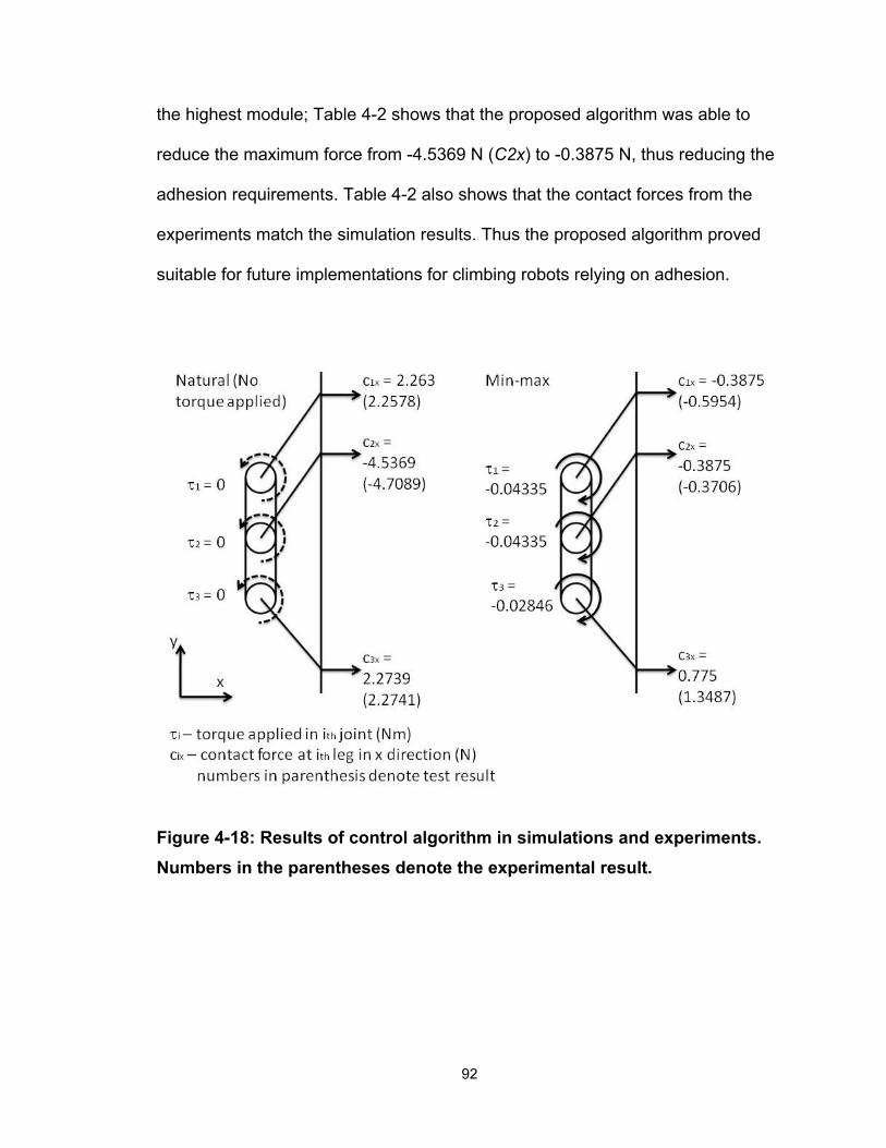
92

the highest module; Table 4-2 shows that the proposed algorithm was able to

reduce the maximum force from -4.5369 N (C2x) to -0.3875 N, thus reducing the

adhesion requirements. Table 4-2 also shows that the contact forces from the

experiments match the simulation results. Thus the proposed algorithm proved

suitable for future implementations for climbing robots relying on adhesion.

Figure 4-18: Results of control algorithm in simulations and experiments. Numbers in the parentheses denote the experimental result.

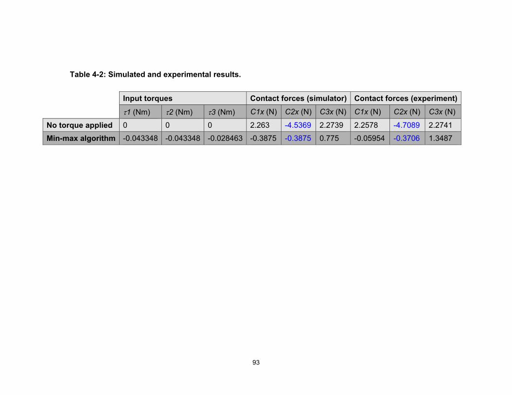
Table 4-2: Simulated and experimental results.

Input torques Contact forces (simulator) Contact forces (experiment)

τ1 (Nm) τ2 (Nm) τ3 (Nm) C1x (N) C2x (N) C3x (N) C1x (N) C2x (N) C3x (N)

No torque applied 0 0 0 2.263 -4.5369 2.2739 2.2578 -4.7089 2.2741

Min-max algorithm -0.043348 -0.043348 -0.028463 -0.3875 -0.3875 0.775 -0.05954 -0.3706 1.3487

93

4.7 Discussion and conclusion

This chapter presented the validation of kinematic analysis and a

preliminary result of controlling adhesion force. Inverse kinematic equations were

used to control the robot’s movement in both simulations and physical robot

tests. The simulation results proved that the equations are correct in the

application so far. Trajectories for a single leg manipulation were validated in

straight-line movements. Robot body manipulation was only tested in a moving

robot platform parallel to a flat surface. Combining these test results led to the

feasibility of the robot walking on level ground and climbing vertical surfaces.

Passive mechanisms should be further investigated to compensate for the error

introduced by manufacturing tolerances of various components.

A power consumption test for optimal release of dry adhesion was

performed. A platform was designed to validate the adhesive’s properties. In

order to keep the supporting feet on the wall, the reaction force between wall and

the peeling foot should be as small as possible. Test results validated the

assumption in a macro-scale thin film adhesive. The test platform proposed here

could be used with modification (e.g., adding another joint to control the

approaching angle) in future foot designs before applying to the climbing robot

and robot posture investigation.

Based on the two preliminary tests, the optimal angle between the leg and

surface was obtained, and it was also proved that the adhesion forces can be

increased by actively controlling the torque of the motors. Tests performed by

using the Min-max algorithm showed that optimal joint torques can maximize

94

preload and minimize contact forces, thus enabling us to take full advantage of

the adhesion properties.

95

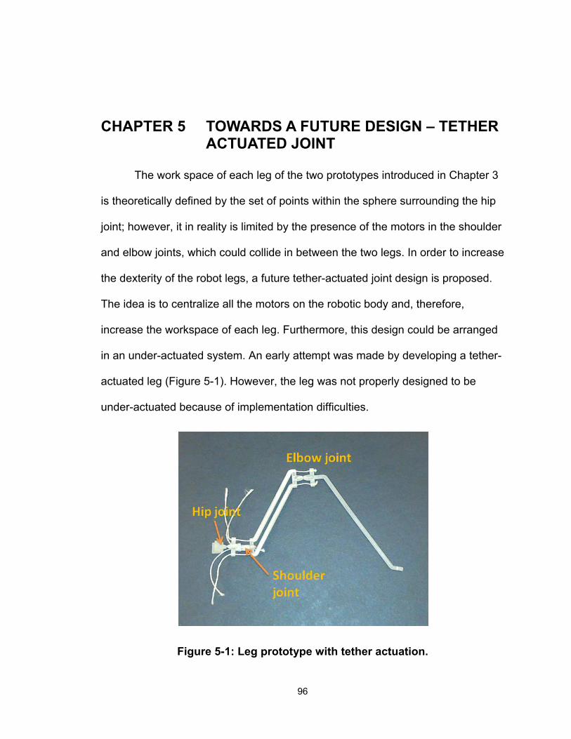
CHAPTER 5 TOWARDS A FUTURE DESIGN – TETHER ACTUATED JOINT

The work space of each leg of the two prototypes introduced in Chapter 3

is theoretically defined by the set of points within the sphere surrounding the hip

joint; however, it in reality is limited by the presence of the motors in the shoulder

and elbow joints, which could collide in between the two legs. In order to increase

the dexterity of the robot legs, a future tether-actuated joint design is proposed.

The idea is to centralize all the motors on the robotic body and, therefore,

increase the workspace of each leg. Furthermore, this design could be arranged

in an under-actuated system. An early attempt was made by developing a tether-

actuated leg (Figure 5-1). However, the leg was not properly designed to be

under-actuated because of implementation difficulties.

Figure 5-1: Leg prototype with tether actuation.

96

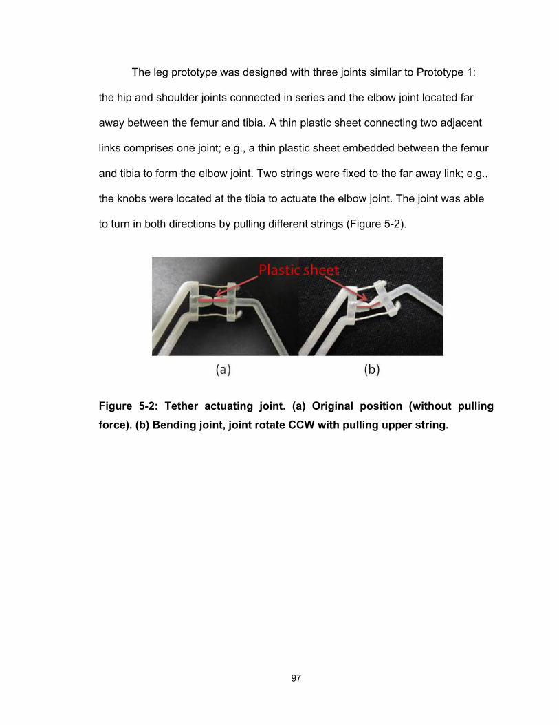
The leg prototype was designed with three joints similar to Prototype 1:

the hip and shoulder joints connected in series and the elbow joint located far

away between the femur and tibia. A thin plastic sheet connecting two adjacent

links comprises one joint; e.g., a thin plastic sheet embedded between the femur

and tibia to form the elbow joint. Two strings were fixed to the far away link; e.g.,

the knobs were located at the tibia to actuate the elbow joint. The joint was able

to turn in both directions by pulling different strings (Figure 5-2).

Figure 5-2: Tether actuating joint. (a) Original position (without pulling force). (b) Bending joint, joint rotate CCW with pulling upper string.

97

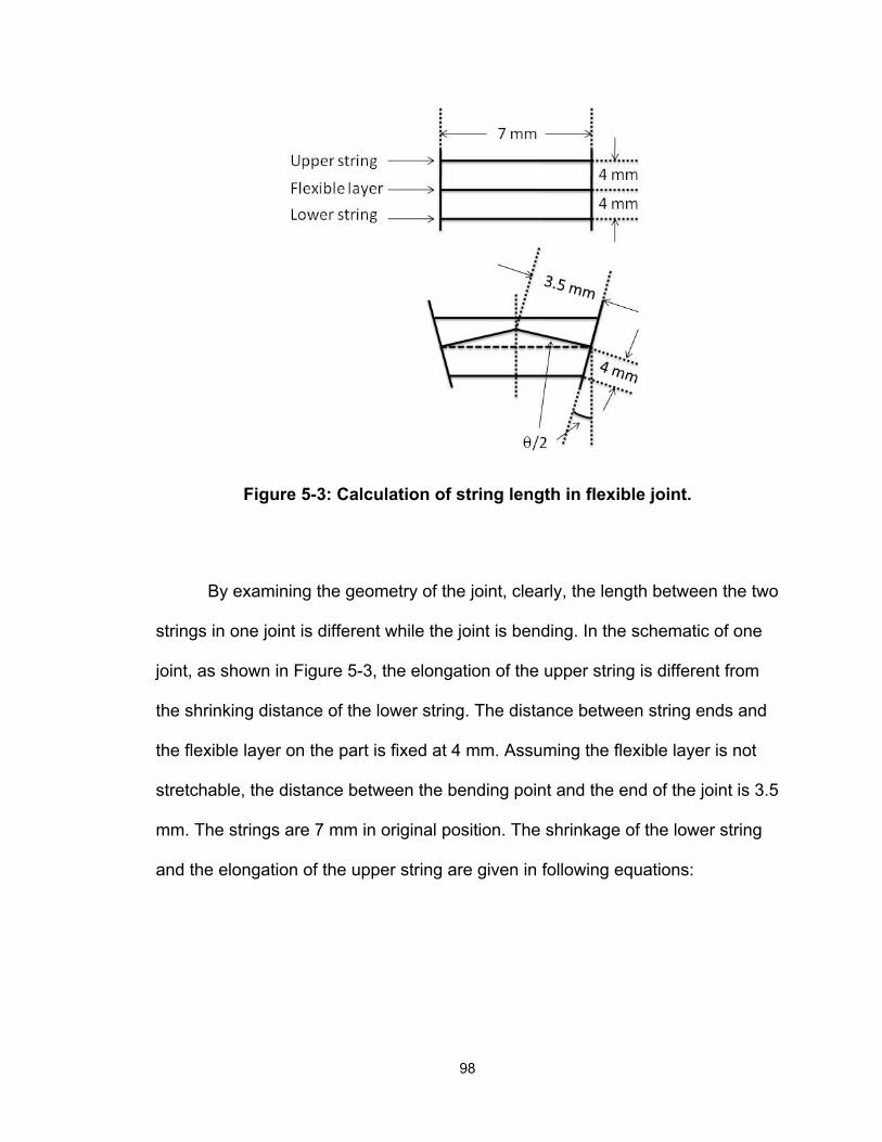
Figure 5-3: Calculation of string length in flexible joint.

By examining the geometry of the joint, clearly, the length between the two

strings in one joint is different while the joint is bending. In the schematic of one

joint, as shown in Figure 5-3, the elongation of the upper string is different from

the shrinking distance of the lower string. The distance between string ends and

the flexible layer on the part is fixed at 4 mm. Assuming the flexible layer is not

stretchable, the distance between the bending point and the end of the joint is 3.5

mm. The strings are 7 mm in original position. The shrinkage of the lower string

and the elongation of the upper string are given in following equations:

98

7 2 3.5 2 4 2 7 7 2 8 2 (5-1)

2 3.5 2 4 2 7 7 2 8 2 7 (5-2)

where θ denotes the angular change in the joint.

(a)

(b)

Figure 5-4: A cam design for pulling strings. (a) Contour of the cam for elongation and shrinkage. (b) A cam used to activate the elbow joint.

99

According to the above equations, a cam was designed to attach to the

rotary motor in order to actuate this specific joint (Figure 5-4). The contour of the

cam was designed to be symmetric to actuate the joint by rotating in both

directions. The hole was attached to the motor shaft, which is housed at the robot

body. Each joint needs a motor to actuate; therefore, the leg needs three cams

attached to the motors. Considering the robot is mounted with six legs in this

configuration, there will be eighteen cams and motors centralized at the body.

The wiring path should be properly designed as it will be difficult to find space for

mounting electronics. However, this design will centralize most of the body mass

(mainly from the motors) at the body. The COM will always be inside the body

volume and, therefore, will be easier to control compared to current prototypes.

Further development of this under-actuated system will decrease the number of

actuators and keep the advantage of a stable COM.

100

CHAPTER 6 CONCLUSIONS AND FUTURE WORK

6.1 Conclusions

Inspired by spiders, the development of a hexapod climbing robot was

introduced in this thesis. Background studies on dry adhesion and climbing

robots were provided. Existing climbing robots using dry adhesion encounter

several problems in mobility, such as turning and transiting different angled

surfaces. The proposed hexapod climbing robot in this research was designed to

solve these problems. Although synthetic dry adhesion at the present stage was

not able to adhere well to rough surfaces, the robot under development was

developed with the potential to climb on various surfaces under different

circumstance.

Motivated by designing such a robot, the mechanical design was inspired

by spiders. The basic configuration of the climbing robot had six legs arranged in

a circular platform, with three revolute actuators in each joint. In order to control

the robot movement as planned, kinematics were studied in order to generate the

joint variables following certain trajectories. Single leg kinematics and robot

platform kinematics were considered in separate cases and afterwards were

combined considering controlling the whole robot. The local ground coordinates

were proposed because the original world coordinates which is fixed to the

ground will become far away from the robot’s coordinates while the robot keeps

101

walking. The introduction of the local ground coordinate provided an alternative

approach for the robot to better cope with nearby terrain changes.

Two prototypes were developed based on the two configurations in

different design approaches. Mechanical and mechatronic design aimed at

developing a miniaturized and robust climbing system were presented. Prototype

1 utilized parts from commercially available servo motors. The electronic boards

of the motors served also as structural components for the robot legs and body,

in order to reduce the robot’s weight. Prototype 2 used all customized electronics

which were selected for their power saving potential. Sensors that produce no

friction and actuators that provide relatively strong torque with a mini gearbox

were used. All the components were small and lightweight, compared to existing

climbing robots. The control strategies were different in both prototypes, while

Prototype 2 required the consideration of much more sophisticated electronic

design.

Based on the kinematic analysis, tests were performed to validate the

equations. Experiments successfully proved the equations were applicable for

the defined tasks, and those test platforms were further utilized to investigate

adhesion and movement. The result of optimized trajectory for peeling the

adhesive was applied to the climbing test. Prototype 1, with attached adhesive,

achieves the goal of climbing a smooth vertical wall.

Several assumptions and considerations were considered during the

investigation of the climbing and adhesion mechanism in order to finally develop

a climbing robot integrated with a synthetic dry adhesive. Our preliminary result

102

shows the potential of achieving the goal of the proposed research. Future work

will focus on improving the performance of the climbing robot from adhesion and

power saving perspectives.

6.2 Future work

6.2.1 Four joints in each leg

While testing the robot climbing a vertical wall, the direction of the

adhesive, which is the angle between adhesive film and the leg stem, changed

every time when a different robot posture was used. Although the silicone glue

provided flexibility for the rotation while the leg attached to the surface, the

approaching angle was fixed and affects the preload and adhesion quality

(attached area). A fourth joint, placed parallel to the shoulder and elbow joints,

might be able to solve this problem. The kinematic configuration, therefore, will

change, and each leg of the robot will become a redundant serial manipulator for

end-effector position control. Joint angles will not be a single solution for a fixed

end effector position. Trajectory planning should be analyzed carefully; by

actively controlling the position of the end effector, the robot might perform better

with the adhesive attached. Considering Prototype 1, the servo controller is able

to connect to a maximum of 32 motors. With the same construction as the

shoulder and elbow joint, the fourth joint can to be added without extra designs.

However, this joint will increase six sets of sensors and actuators, which will

increase both the complexity and weight of the climbing robot. The electronics

will also become more complicated by significantly increasing the number of

components, especially in Prototype 2. On the other hand, reducing actuators by

103

introducing an under-actuated system might compensate for this extra

complexity.

6.2.2 Joints with tether actuation

As described in Chapter 5, an under-actuated system may be useful for

future variations on this climbing robot. There are existing robot hands and tether

actuated robotic systems for reference, e.g. the famous Utah/MIT dexterous

hand, Stanford/JPL finger et al. The tether actuated system, or tendon driven

system in bio-mimetic terms, is also inspired by nature. Spiders use both tendon

and hydraulic tubes to actuate the joints in their legs [36]. By further investigating

the spider actuation system, the design of future climbing robots might be able to

reduce the number of actuators and, therefore, reduce the robot weight and

improve climbing capabilities.

104

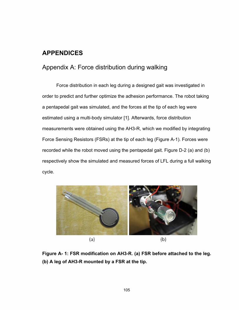
APPENDICES

Appendix A: Force distribution during walking

Force distribution in each leg during a designed gait was investigated in

order to predict and further optimize the adhesion performance. The robot taking

a pentapedal gait was simulated, and the forces at the tip of each leg were

estimated using a multi-body simulator [1]. Afterwards, force distribution

measurements were obtained using the AH3-R, which we modified by integrating

Force Sensing Resistors (FSRs) at the tip of each leg (Figure A-1). Forces were

recorded while the robot moved using the pentapedal gait. Figure D-2 (a) and (b)

respectively show the simulated and measured forces of LFL during a full walking

cycle.

Figure A- 1: FSR modification on AH3-R. (a) FSR before attached to the leg. (b) A leg of AH3-R mounted by a FSR at the tip.

105

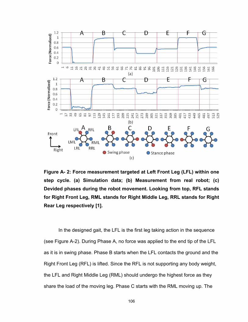
Figure A- 2: Force measurement targeted at Left Front Leg (LFL) within one step cycle. (a) Simulation data; (b) Measurement from real robot; (c) Devided phases during the robot movement. Looking from top, RFL stands for Right Front Leg, RML stands for Right Middle Leg, RRL stands for Right Rear Leg respectively [1].

In the designed gait, the LFL is the first leg taking action in the sequence

(see Figure A-2). During Phase A, no force was applied to the end tip of the LFL

as it is in swing phase. Phase B starts when the LFL contacts the ground and the

Right Front Leg (RFL) is lifted. Since the RFL is not supporting any body weight,

the LFL and Right Middle Leg (RML) should undergo the highest force as they

share the load of the moving leg. Phase C starts with the RML moving up. The

106

LFL was not adjacent or opposite to the moving leg (RML) and has the same

load as all legs are in contact to the ground. Data in Phase D shows that the

force decreased when the opposite leg was in the swing phase. Phase E and F

had a similar effect on Phase C and B. Phase G represents the robot body

moving forward with all legs attached to the ground. Since the FSRs are not

suitable to show the absolute value of the force, both the simulated and

experimental data were normalized to better compare the trends of interested

forces. We observed that (a) the moving leg bears no force and its opposite leg

bears minor force, (b) two adjacent legs undergo the highest load during the

movement, (c) forces at the non-adjacent and non-opposite legs were identical to

the stance phase. Test results showed that the simulation was consistent to the

realistic force distribution of the robot; therefore, future analyses predicting loads

during vertical climbing or upside-down locomotion could accurately be

performed.

The FSRs (Figure A-1 (a)) we used was manufactured by Interlink

electronics [40]. Relationship between applied force and output voltage is not

linear according to datasheet. A circuit for integrating the FSRs proposed by

Lynxmotion [41] is utilized in force distributing test. Output voltage and the

applied force was calibrated using a customized test. The relationship between

force and voltage is shown in Figure A-3. Weights were put on the FSR and the

corresponding output voltage was recorded.

107

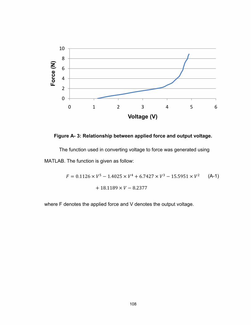
0

2

4

6

8

10

0 1 2 3 4 5 6

Forc

e (N

)

Voltage (V)

Figure A- 3: Relationship between applied force and output voltage.

The function used in converting voltage to force was generated using

MATLAB. The function is given as follow:

0.1126 1.4025 6.7427 15.5951

18.1189 8.2377

(A-1)

where F denotes the applied force and V denotes the output voltage.

108

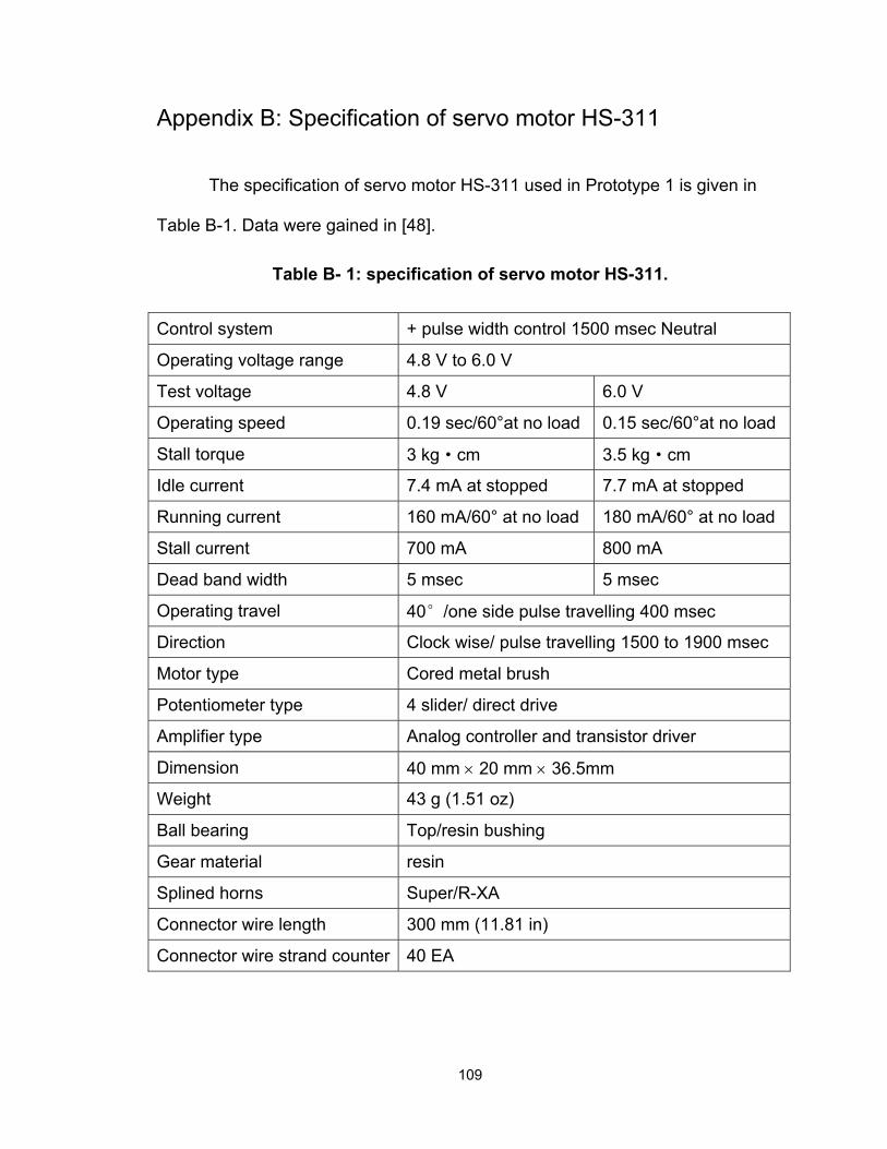
109

Appendix B: Specification of servo motor HS-311

The specification of servo motor HS-311 used in Prototype 1 is given in

Table B-1. Data were gained in [48].

Table B- 1: specification of servo motor HS-311.

Control system + pulse width control 1500 msec Neutral

Operating voltage range 4.8 V to 6.0 V

Test voltage 4.8 V 6.0 V

Operating speed 0.19 sec/60°at no load 0.15 sec/60°at no load

Stall torque 3 kg·cm 3.5 kg·cm

Idle current 7.4 mA at stopped 7.7 mA at stopped

Running current 160 mA/60° at no load 180 mA/60° at no load

Stall current 700 mA 800 mA

Dead band width 5 msec 5 msec

Operating travel 40°/one side pulse travelling 400 msec

Direction Clock wise/ pulse travelling 1500 to 1900 msec

Motor type Cored metal brush

Potentiometer type 4 slider/ direct drive

Amplifier type Analog controller and transistor driver

Dimension 40 mm × 20 mm × 36.5mm

Weight 43 g (1.51 oz)

Ball bearing Top/resin bushing

Gear material resin

Splined horns Super/R-XA

Connector wire length 300 mm (11.81 in)

Connector wire strand counter 40 EA

Appendix C: Specification of mini-motor GH6124S

The mini-motor GH6124S used in Prototype 1 is manufactured by Gizmo’s

zone [43]. In the same series, GH612, from the same manufacturer, the

GH6124S has the highest gear ratio in the gearbox. The diameter of the motors

in this series is 6 mm. Mechanical details and general specification of GH612

series are given in Table C-1 for comparison. The technical detail of GH612

series motor is given in Table C-2. Data in both tables are gained from the

manufacturer [42].

110

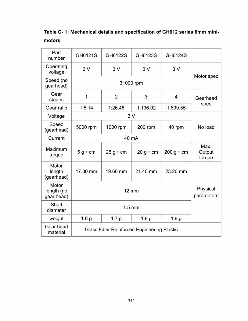
Table C- 1: Mechanical details and specification of GH612 series 6mm mini-motors

Part number GH6121S GH6122S GH6123S GH6124S

Operating voltage 3 V 3 V 3 V 3 V

Motor spec Speed (no gearhead) 31000 rpm

Gear stages 1 2 3 4 Gearhead

spec Gear ratio 1:5.14 1:26.45 1:136.02 1:699.55

Voltage 3 V

No load Speed (gearhead) 5000 rpm 1000 rpm 200 rpm 40 rpm

Current 40 mA

Maximum torque 5 g·cm 25 g·cm 120 g·cm 200 g·cm

Max. Output torque

Motor length

(gearhead) 17.80 mm 19.60 mm 21.40 mm 23.20 mm

Physical parameters

Motor length (no gear head)

12 mm

Shaft diameter 1.5 mm

weight 1.6 g 1.7 g 1.8 g 1.9 g

Gear head material Glass Fiber Reinforced Engineering Plastic

111

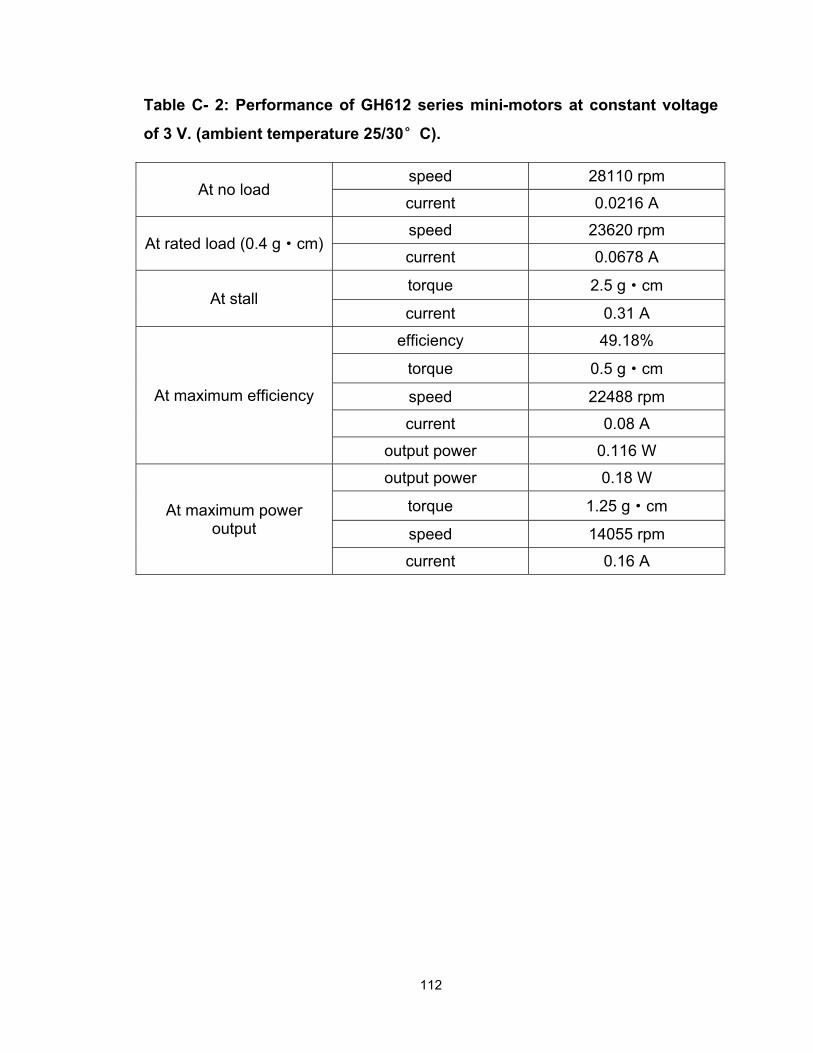
112

Table C- 2: Performance of GH612 series mini-motors at constant voltage

of 3 V. (ambient temperature 25/30°C).

At no load speed 28110 rpm

current 0.0216 A

At rated load (0.4 g·cm) speed 23620 rpm

current 0.0678 A

At stall torque 2.5 g·cm

current 0.31 A

At maximum efficiency

efficiency 49.18%

torque 0.5 g·cm

speed 22488 rpm

current 0.08 A

output power 0.116 W

At maximum power output

output power 0.18 W

torque 1.25 g·cm

speed 14055 rpm

current 0.16 A

Appendix D: Specification of mini-motor GM15

The mini-motor GM15 used in Prototype 2 is manufactured by Solarbotics

[47]. Specification of GM15 is summarized in Table D-1.

Table D- 1: Specification of GM15 mini-motor [47].

Gear ratio 1:25

Dimensions 20.1 mm × 6 mm × 6 mm (wire length 25 mm)

Weight 1.3 g

Test voltage 3 V 6 V

Unloaded speed 920 rpm 1550 rpm

Unloaded current 100 mA 200 mA

Stall current 210 mA 350 mA

Stall torque 35.28 g·cm 69.33 g·cm

113

Appendix E: Relationship between output voltage and rotary

position of HMC1512

From an application note from Honey well [39], the HMC1512 is able to

sense 180 degrees of rotary displacement using the following set of equations:

∆ ∆ 2 ∆ (E-1)

∆ 2

∆ 2

(E-2)

(E-3)

where Vs is supplied voltage to the chip, S is the material constant which

is set to 12 mV/V, θ is the reference of the magnetic field angle. The first

equation denotes the relationship between the differentiated output voltage and

magnetic angle, while the two equations below represent the individual bridge

output with respect to the magnetic field angle.

Sensor test result in Figure 3-10 match the waveform graph the

manufacturer provided in 135 degrees of displacement. Instead of equations (E-

1) to (E-3), equations (3-1) and (3-2) were used to transform between output

voltage and angular displacement. The modified equations in Chapter 3 are

convenient to utilize and simplified in two situations, for they are easily integrated

in the control node in LabVIEW.

114

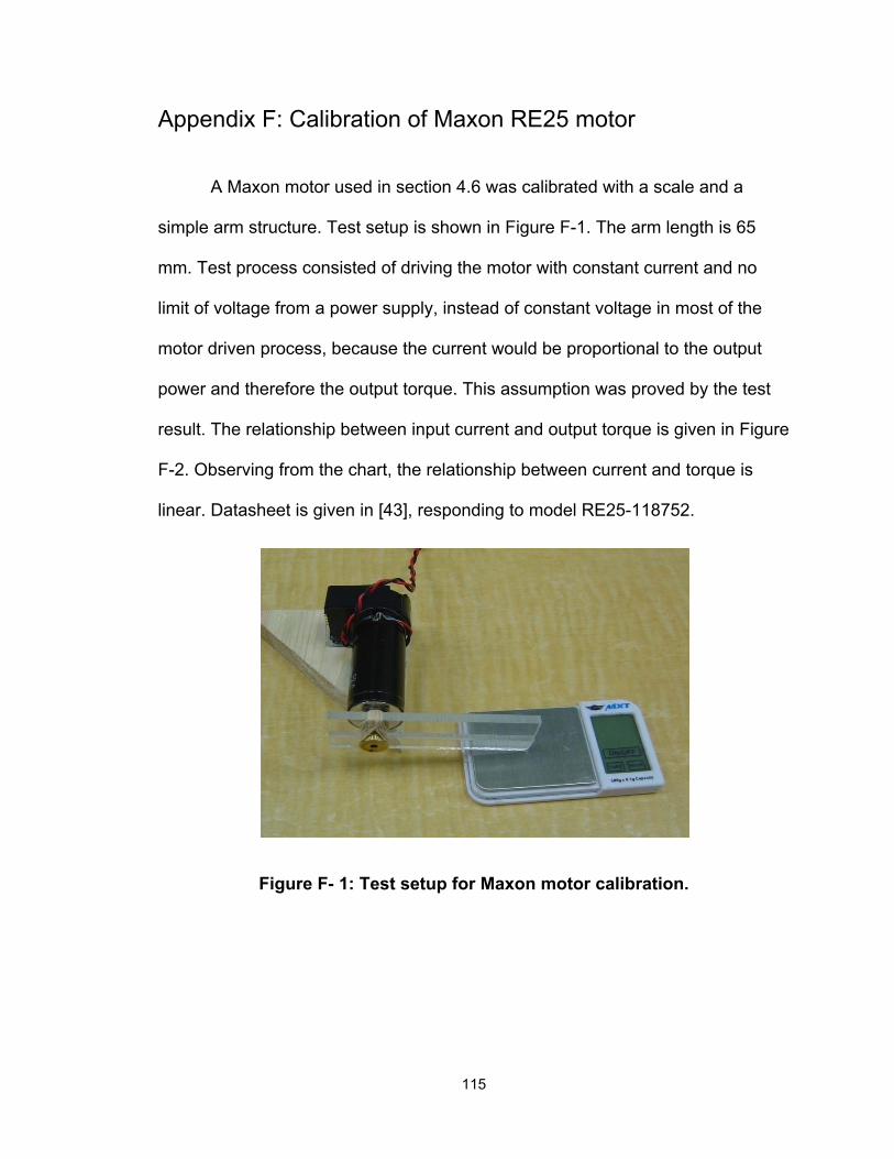
Appendix F: Calibration of Maxon RE25 motor

A Maxon motor used in section 4.6 was calibrated with a scale and a

simple arm structure. Test setup is shown in Figure F-1. The arm length is 65

mm. Test process consisted of driving the motor with constant current and no

limit of voltage from a power supply, instead of constant voltage in most of the

motor driven process, because the current would be proportional to the output

power and therefore the output torque. This assumption was proved by the test

result. The relationship between input current and output torque is given in Figure

F-2. Observing from the chart, the relationship between current and torque is

linear. Datasheet is given in [43], responding to model RE25-118752.

Figure F- 1: Test setup for Maxon motor calibration.

115

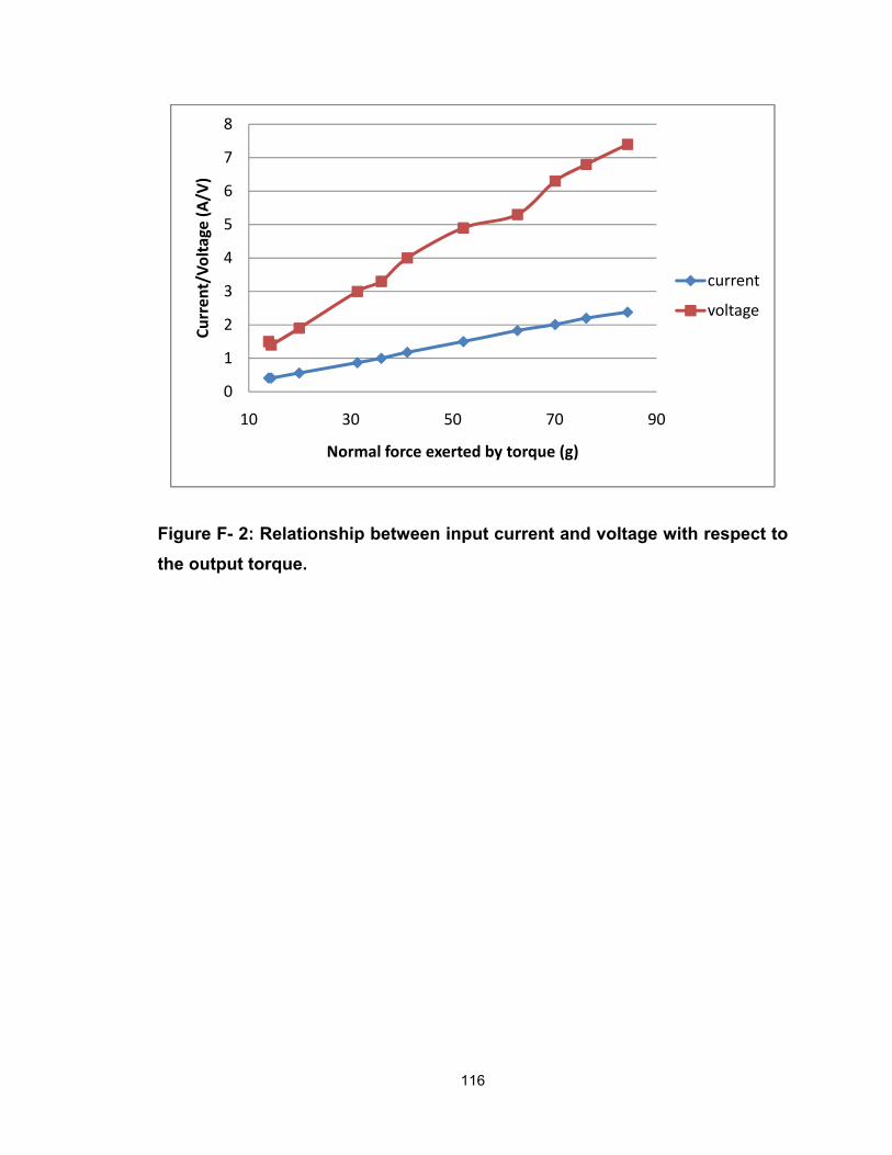
0

1

2

3

4

5

6

7

8

10 30 50 70 90

Curren

t/Vo

ltage (A/V

)

Normal force exerted by torque (g)

current

voltage

Figure F- 2: Relationship between input current and voltage with respect to the output torque.

116

BIBLIOGRAPHY5

[1] Y. Li, A. Ahmed, C. Wu, C. Menon, “Preliminary Analysis of a Legged Robot Designed to Climb Vertical Surfaces”, 2009 IEEE Toronto International Conference - Science and Technology for Humanity, Toronto, Canada, 2009.

[2] K. Autumn, M. Sitti, Y. A. Liang, A. M. Peattle, W. R. Hansen, S. Sponberg, T. W. Kenny, R. Fearing, J. N. Israelachvili, and R. J. Full, "Evidence for van der waals adhesion in gecko setae," PNAS, vol. 99, pp. 12252-12256, 2002.

[3] S. Kim and M. Sitti, "Biologically inspired polymer microfibers with spatulate tips as repeatable fibrillar adhesives," Applied Physics Letters, vol. 89, pp. 261911 1-3, 2006.

[4] H. Yao, H, Gao, “Mechanics of robust and releasable adhesion in biology: Bottom-up designed hierarchical structures of gecko,” Journal of the Mechanics and Physics of Solids, vol 54 (6), pp. 1120-1146, 2006.

[5] C. Menon, N. Lan, D. Sameoto, “Towards a methodical approach to implement biomimetic paradigms in the design of robotic systems for space applications”, Applied Bionics and Biomechanics, pp.1–13, 2009.

[6] D. Sameoto, Y. Li, C. Menon, “Multi-scale compliant foot designs and fabrication for use with a spider-inspired climbing robot”, Journal of Bionic Engineering, Vol. 05, No. 03, pp. 189-19, 2008.

[7] D. Sameoto, Y. Li, C. Menon, “Micromask Generation for Polymer Morphology Control: Nanohair Fabrication for Synthetic Dry Adhesives”, Advances in Science and Technology, Trans Tech Publications, Vol. 54 pp 439-444, 2008.

[8] M. Greuter, G. Shah, G. Caprari, F. Tache, R. Siegwart, and M. Sitti, "Toward micro wall-climbing robots using biomimetic fibrillar adhesives," presented at Proceedings of the 3rd International Symposium on Autonomous Mini Robots for Research and Edutainment, Awara-Spa, Fukui, 2005.

5 Publications highlighted throughout are results of this thesis work.

117

[9] K. A. Daltorio, S. Gorb, A. Peressadko, A. D. Horchler, R. E. Ritzmann, and R. D. Quinn, "A robot that climbs walls using microstructured polymer feet," Proceedings of the Eighth International Conference on Climbing and Walking Robots and the Support Technologies for Mobile Machines, pp. 131-138, 2005.

[10] O. Unver, A. Uneri, A. Aydemir, and M. Sitti, "Geckobot: a gecko inspired climbing robot using elastomer adhesives," Proceedings of the International Conference on Robotics and Automation, pp. 2329-2335, 2006.

[11] S. Kim, M. Spenko, S. Trujillo, B. Heyneman, M. V, and M. Cutkosky, "Whole body adhesion: heirarchical, directional and distributed control of adhesion forces for a climbing robot," IEEE Conference on Robotics and Automation, pp. 1268-1273, 2007.

[12] M. Murphy, M. Sitti, “Waalbot: an agile small-scale wall climbing robot ustilizing dry elastomer adhesives”, IEEE/ASME transactions on Mechatronics, vol. 12 (3), pp. 330-338, 2007.

[13] C. Menon, M. Murphy, and M. Sitti, "Gecko inspired surface climbing robots," IEEE International Conference on Robotics and Biomimetics, Shenyang, China, 2004.

[14] C. Menon, M. Murphy, M. Sitti, N. Lan, “Space exploration - towards new advanced bioinspired climbing robots, in (M.K. Habib Ed.) Bioinspiration and Robotics - Walking and Climbing Robots”, Advanced Robotic Systems International and I-Tech, pp544, 2007.

[15] C. Menon, M. Sitti, “A Biomimetic Climbing Robot Based on the Gecko”, Journal of Bionic Engineering, Elsevier, Vol. 3, No. 03, pp. 115-125. 2006.

[16] A. B. Kesel, A. Martin and T. Seidl, “Getting a grip on spider attachement: an AFM approach to microstructure adhesion in arthropods”, Smart Materials and Structures, vol 13, pp 512-518, 2004.

[17] S. Niederegger, S. N. Gorb, “Friction and adhesion in the tarsal and metatarsal scopulae”, J Comp Physiol A (2006) 192: 1223-1232.

[18] K. Autumn, Y. A. Liang, S. T. Hsieh, W. Zesch, W. P. Chan, T. W. Kenny, R. Fearing, and R. J. Full, "Adhesive force of a single gecko hair," Nature, vol. 405, pp. 681-685, 2000.

[19] D. Campolo, S. Jones, and R. S. Fearing, "Fabrication of gecko foot-hair like nano structures and adhesion to random rough surfaces," presented at Nanotechnology 2003, San Fransisco, CA, 2003.

[20] M. Sitti and R. S. Fearing, "Synthetic gecko foo-hair micro/nano-structures as dry adhesives," Journal of Adhesion Science and Technology, vol. 18, pp. 1055-1074, 2003.

118

[21] A. K. Geim, S. V. Dubonos, I. V. Grigorieva, K. S. Novoselov, A. A. Zhukov, and S. Y. Shapoval, "Microfabricated adhesive mimicking gecko foot-hair," Nature Materials, vol. 2, pp. 461-463, 2003.

[22] D. Santos, S. Kim, M. Spenko, A. Parness, M. Cutkosky, “Directional Adhesive Sturctures for Controlled Climbing on Smooth Vertical Surfaces”, 2007 IEEE International Conference on Robotics and Automation, pp1262-1267, 2007.

[23] B. Aksak, M. P. Murphy and M. Sitti, “Gecko Inspired Micro-Fibrillar Adhesives for Wall Climbing Robots on Micro/Nanoscale Rough Surfaces”, 2008 IEEE International Conference on Robotics and Automation, pp3058-3063, 2008.

[24] D. Sameoto, C. Menon, “Direct molding of dry adhesives with anisotropic peel strength,” Journal of Micromechanics and Microengineering, 2009.

[25] S. Kim, A. T. Asbeck, M. Cutkosky, and W. R. Provancher, "Spinybot II: climbing hard walls with compliant microspines," Proc. of 12th Int. Conf. on Advanced Robotics, pp. 601-606, 2005.

[26] A. Saundersa, D.I. Goldmanb, R.J. Fullb, M. Buehlera, “The RiSE Climbing Robot: Body and Leg Design,” Proc. of SPIE Vol. 6230, 623017, 2006.

[27] M. J. Randall, “Adaptive neural control of walking robots,” London: Professional Engineering, 2001, pp.2.

[28] Y. Li, D. Sameoto, C. Menon, “Properties Validation of an Anisotropic Dry Adhesion Designed for Legged Climbing Robots”, 2009 IEEE International Conference on Robotics and Biomimetics, 2009.

[29] Z. Wang, X. Ding, A. Rovetta, “Structure Design and Locomotion Analysis of a Novel Robot for Lunar Exploration”, 12th IFToMM World Congress, Besançon , France, June18-21, 2007.

[30] S. Kim and M. Sitti, "Biologically inspired polymer microfibers with spatulate tips as repeatable fibrillar adhesives," Applied Physics Letters, vol. 89, pp. 261911 1-3, 2006.

[31] H. Yao, H, Gao, “Mechanics of robust and releasable adhesion in biology: Bottom-up designed hierarchical structures of gecko,” Journal of the Mechanics and Physics of Solids, vol 54 (6), pp. 1120-1146, 2006.

[32] D. Sameoto, Y. Li, C. Menon, “Multi-scale compliant foot designs and fabrication for use with a spider-inspired climbing robot”, Journal of Bionic Engineering, Vol. 05, No. 03, pp. 189-19, 2008.

119

[33] D. Sameoto, Y. Li, C. Menon, “Micromask Generation for Polymer Morphology Control: Nanohair Fabrication for Synthetic Dry Adhesives”, Advances in Science and Technology, Trans Tech Publications, Vol. 54 (2008) pp 439-444.

[34] C. Menon, Y. Li, D. Sameoto, C. Martens, “Abigaille-I: towards the development of a spider-inspired climbing robot for space use,” 2008 2nd IEEE RAS & EMBS International Conference on Biomedical Robotics and Biomechatronics. BioRob 2008, pp. 384-9, 2008.

[35] K. Kendall, “Thin-film peeling – the elastic term,” Journal of Physics D (Applied Physics), pp. 1449-1452, 1975.

[36] R. F. Foelix, “Biology of Spiders,” New York: Oxford University Press; 1996.

[37] Claire W., Spider robot system design, Report for ENSC494 Special Project, School of Engineering Science, SFU, 2008.

[38] I. Pretto, Y. Li, C. Menon, S. Cocuzza (in preparation) Strategies for optimizing adhesion force during robotic vertical climbing. To be submitted to IEEE Transaction on Robotics.

[39] Magnetic Displacement Sensors HMC1501/1512, URL: http://www.magneticsensors.com/datasheets/hmc1501-1512.pdf.

[40] Interlink electronics, Force sensing resistor (FSR), URL: http://www.interlinkelectronics.com/force_sensors/technologies/fsr.html.

[41] James Frye, Hexapod Foot Sensor Assembly Guide, Lynxmotion Inc., URL: http://www.lynxmotion.com/images/html/build127.htm.

[42] Spec sheet of GH612 series 6mm mini motor, URL: http://www.gizmoszone.com/shopping/storepro5/html/pages/612metaldatasheet.pdf

[43] Maxon precision motors, URL: http://shop.maxonmotor.com/ishop/article/article/118752.xml.

[44] Manual of SSC-32, URL: http://www.lynxmotion.com/images/html/build136.htm.

[45] Specification of Visual Sequencer, URL: http://www.lynxmotion.com/Product.aspx?productID=443&CategoryID=15.

[46] Schematic of BlueSMiRF, URL: http://www.sparkfun.com/datasheets/RF/BlueSMiRF-Gold-ChipAnt-v1.pdf.

120

121

[47] Resource of GM15, URL: http://www.solarbotics.com/products/gm15/resources/.

[48] Specification of servo motor HS311, URL: http://www.hitecrcd.com/product_file/file/45/HS311.pdf.

[49] Specification of plastic material of 3D printer VisiJet® SR-200, URL: http://www.simt.com/rpc/pdf/23100-S02-02_A_MSDS_US_English_SR200.pdf