preliminary analysis of forest stand disturbances in

FORMATH Vol. 18 (2019), DOI:10.15684/formath.18.001

c⃝2019 FORMATH Research Group

Scientific Category

Preliminary Analysis of Forest Stand Disturbances in CoastalGeorgia (USA) Using Landsat Time Series Stacked Imagery

Shingo Obata1∗, Chris J. Cieszewski1, Pete Bettinger1, Roger C. Lowe III1, SergioBernardes2

Abstract: A determination of forest characteristics across broad areas is of great concern to the forest industryin the southern United States, as timber supply decisions can be based on opportunities, or lack ofthereof, across all wood procurement areas. This is important in areas such as the southern UnitedStates, where the land ownership distribution is highly fragmented and where no general comprehensivesource of forest data exists other than the low-intensity USDA Forest Service FIA surveys. In an effortto describe forest characteristics along the lower Coastal Plain of the State of Georgia (USA), weutilized a time series of Landsat data and an algorithm that assesses an integrated forest Z score.The methodology was used to create disturbance maps for over 30 years that represent the year ofdisturbance for specific locations. The overall accuracy was 52% when all years were considered, andapproximately 70% from 1991 forward. Preliminary findings showed moderate levels of accuracy whendetermining ages for current forests, most of which are even-aged nature stands. Further modificationsto the process were necessary to adapt to the unique conditions of study region. The modeling processalso prompted several areas for future refinement, including improvement of the temporal resolution ofthe analysis by using all the available Landsat imagery and detection of the regeneration that normallyoccurs several years after disturbances.

Keywords: forest planning, forest resource management, land cover change analysis, mathematical modeling,remote sensing

1. Introduction

Acquisition of information regarding the state of natural resource availability and their charac-teristics can be one of the most expensive components of forest management (Bettinger et al. 2017).Satellite technology can provide a cost-effective source of spatial information and can facilitate pro-cesses that allow one to estimate various natural resource characteristics needed for the planningand management of forests, sustainability analysis (Cieszewski et al. 2004; Liu and Cieszewski 2009)and biomass supply assessment (Cieszewski et al. 2011). Of the many satellites currently in oper-ation, those belonging to the Landsat series are frequently used for terrestrial resource assessments/ monitoring due to the long life of the program (first launched in 1972) do not change the char-acteristics of the platform: orbit, sensors, temporal resolution, consistent footprint, and moderatespatial resolution (Roy et al. 2014). Along with the growing power and availability of computingand software technology, the evolving body of scientific research is continuously revealing growingpotential to estimate more detailed forest information using satellite imagery. This progressionin applied science has evolved beyond static analyses of single satellite images to spatiotemporalanalyses of series (stacks) of images captured at different points in time. Time series analysis ofremotely-sensed data can help identify forest disturbance, which is one critically important processin an assessment of the current state of forest resources across broad landscapes. Dating disturbanceevents by using remote sensing can facilitate the determination of forest age and of current stage offorest development. In this paper, the term “disturbance” is used to refer to abrupt loss of forestcover in an area. This includes any types of the causes that lead the change. Disturbance is causedby two types of events. The first one is natural disturbance such as forest fire and windthrow. Theother is anthropogenic disturbance including major harvesting that clears all the foreststand andminor harvesting that leaves majority of the forest cover.

With temporal trajectory-based image analysis (change detection), changes in land use can bedetected with a help of an algorithm that assesses a time series of satellite images to locate changesin the spectral signatures of arbitrary locations within a landscape (Brooks et al. 2014). TheVegetation Change Tracker (VCT), for example, uses an integrated forest score (IFZ) as a metric to

Received July 24, 2018; Accepted Oct. 2, 20181Warnell School of Forestry and Natural Resources, University of Georgia, USA2Center for Geospatial Research, University of Georgia, USA∗Corresponding Author: [email protected]

1

Obata et al.

distinguish forested areas from others areas at the resolution of a single pixel (Huang et al. 2009).Application of these types of algorithms enables the development of a map, which specifies theyears of stand disturbances. LandTrendr is another example algorithm for automatic detection ofchanges in land use (Kennedy et al. 2010). Other models (e.g., Vogelmann et al. 2012; Jin et al.2013) share common characteristics: stacking annual images captured during a specific season ofthe year, using one or more indices for detection of changes, and comparing results with adjacentyears to verify the changes. The novelty of this kind of research is of great relevance to forestmanagement. For example, Brooks et al. (2014) used statistical process control tools to detectnot only major disturbances (final harvests) but also minor disturbances, such as thinnings. AndZhu et al. (2015) developed an algorithm to remove seasonal effects from the analysis of satelliteimagery. Further, the North American Carbon Program created North American Forest Dynamics(NAFD) products which are a spatially explicit disturbance detection maps for conterminous UnitedStates between 1986 and 2010. NAFD product is comprised of 25 annual and two-time integratedforest disturbance map that shows the specific year of disturbance with 30-meter spatial resolution(Goward et al. 2015).

The objective of this research was to describe the current age class distribution of forests in thelower Coastal Plain of the State of Georgia, an area where forests are managed mainly througheven-aged methods, and where forests are intermixed with other land uses. In this paper we presentthe comprehensive explanation of the work that was briefly summarized in Obata (2018). A long(33 year) time series of Landsat imagery was used to determine the date of the most recent majorforest disturbance (final harvest). The forested and agricultural settings in this region include acomplex interspersion of croplands (e.g., onions), pasture, conifer plantations, deciduous bottom-lands, cypress (Taxodium) forests, and mixed species stands of trees that are managed by publicagencies, private landowners, and the U.S. military. This landscape heterogeneity, along with thevariety of land management objectives that follow, present both challenge and opportunity to thosewho seek to describe the current state of forests. While previous research has illustrated sophisti-cated algorithms for estimating disturbance years, most do not utilize Landsat 8 OLI imagery, whichstarted acquiring images in 2013. Landsat 8 OLI shares common characteristics with Landsat 5 TMin most aspects, yet there is a difference in band centers, where wavelengths located at the centerof the each band in Landsat 8 are different than those of Landsat 5. This difference may result ininconsistencies of the disturbance / regeneration map derived from the imagery. Therefore, it is achallenge to the current research to develop an up-to-date disturbance map for our Coastal Plainstudy site by combining multiple years of Landsat 5 TM and Landsat 8 OLI satellite imagery.

2. Methodology

2.1. Study area

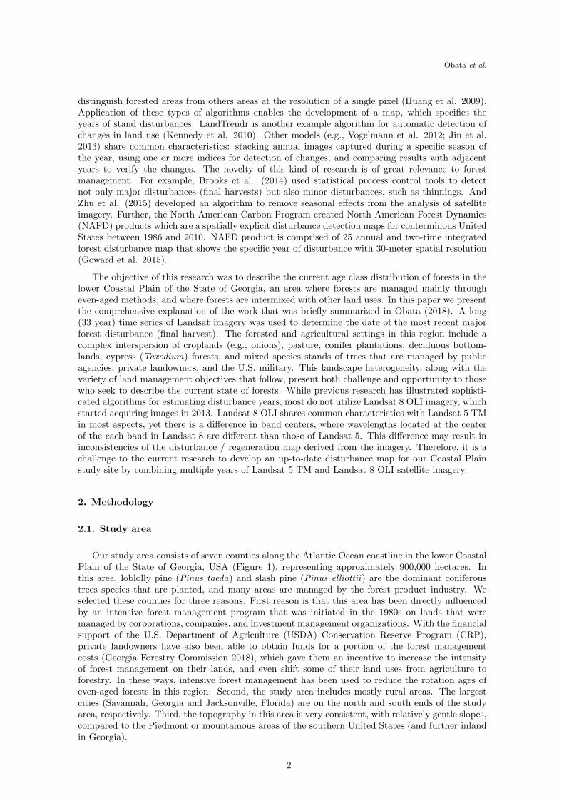
Our study area consists of seven counties along the Atlantic Ocean coastline in the lower CoastalPlain of the State of Georgia, USA (Figure 1), representing approximately 900,000 hectares. Inthis area, loblolly pine (Pinus taeda) and slash pine (Pinus elliottii) are the dominant coniferoustrees species that are planted, and many areas are managed by the forest product industry. Weselected these counties for three reasons. First reason is that this area has been directly influencedby an intensive forest management program that was initiated in the 1980s on lands that weremanaged by corporations, companies, and investment management organizations. With the financialsupport of the U.S. Department of Agriculture (USDA) Conservation Reserve Program (CRP),private landowners have also been able to obtain funds for a portion of the forest managementcosts (Georgia Forestry Commission 2018), which gave them an incentive to increase the intensityof forest management on their lands, and even shift some of their land uses from agriculture toforestry. In these ways, intensive forest management has been used to reduce the rotation ages ofeven-aged forests in this region. Second, the study area includes mostly rural areas. The largestcities (Savannah, Georgia and Jacksonville, Florida) are on the north and south ends of the studyarea, respectively. Third, the topography in this area is very consistent, with relatively gentle slopes,compared to the Piedmont or mountainous areas of the southern United States (and further inlandin Georgia).

2

Forest Stand Disturbances in Coastal Georgia (USA)

Figure 1. Study area.

2.2. Training data

We used the Landsat 5 TM and Landsat 8 OLI imagery to develop the training data set forthe classification process as described below. The development was subject to two conditions: (i)the imagery needed to be captured during the heart of the growing season, which we assumed tobe from the beginning of June to the end of August; and (ii) the imagery needed to be capturedbetween 1984 and 2016. Imagery from 2012 was lacking because neither Landsat 5 nor Landsat 8was in operation during this year. Landsat 7 data could have been used for 2012, however, due tothe failure of the scan line corrector, Landsat 7 data suffer from significant data gaps (Chen et al.2011).

The images were downloaded via EarthExplorer (U.S. Geological Survey 2017); for each yeara single image with the least cloud cover was selected to represent it. We used the C functionof the mask (CFMask) band to remove the effect of clouds (presence and shadows). For pixelsrepresenting water, we applied criteria to mask a pixel when its normalized difference vegetationindex (NDVI) was less than 0.5 and when the surface reflectance value from the near infraredband was less than 0.15. After performing these processes, we visually inspected the quality of theresulting imagery, and decided to exclude the 1993 scene, as the processes failed to eliminate thin,cirrus clouds correctly.

2.3. Reference data

To verify the accuracy of the created forest age map, we used as reference images from GoogleEarth, Landsat 5 TM and Landsat 8 OLI imagery. Google Earth was the primary source of referencedata for the accuracy assessment for more recent years, as the frequency and quality of high-resolution imagery is greater in the last 15 years than before that. We used Landsat imagery forverification of disturbances for earlier years in our time frame (2000 and before). Annual mosaicsof Landsat imagery were created using Google Earth Engine in an effort to acquire cloud-freerepresentations of the landscape. To create annual mosaics, imagery selected to conduct classificationwere not used so that training data and reference data are not mixed each other. These mosaics wereused to verify whether disturbances had occurred during the accuracy assessment process (describedbelow).

2.4. Forest disturbance detection method

The algorithm we developed computed the Integrated Forest Z-score (IFZ value) to detect majorforest disturbances. The IFZ value is a common index (Huang et al. 2010) for this purpose and canbe interpreted as the normalized distance between a pixel value of multi-spectral satellite imagery

3

Obata et al.

and the value of a previously identified, reference forest pixel. When a small IFZ value is producedfor a given year, this suggests an area of relatively stable mature forest. Large IFZ values, onthe other hand, indicate areas where major disturbances have recently occurred. The IFZ valueis computed using the mean and standard deviation of identified forest regions within the satelliteimagery. An identified forest region is a group of pixels which were manually selected to representforest areas. Calculation of the IFZ value for each pixel within an image begins with the calculationsof stand Z-score (FZjik) for each pixel j in each band i for each year k.

[1] FZjik =bjik − bikSDik

∀i, j, k

where:bjik= surface reflectance value of pixel j in band i during year kbik= the mean surface reflectance of forest regions of training areas in band i during year kSDik= the standard deviation of surface reflectance for forest regions of training areas in band iduring year k

Each FZjik is then integrated into a single scalar value for each pixel j during each year k,IFZik, using the following formula:

[2] IFZjk =

√∑NBi=1(FZjik)2

NB∀j, k

Where: NB = the number of bands used

Three bands (red, shortwave infrared-1, and shortwave infrared-2) were used to determine theIFZ value. The actual band numbers used in this computation were bands 3, 5 and 7 (Landsat 5)and bands 4, 6 and 7 (Landsat 8). In calculating the mean and standard deviation values for forestregions, 15 training areas were selected to represent coniferous forests and another 15 training areaswere selected to represent broadleaf forests. The area of each individual training region was about100 ha.

2.5. Image classification

The classification algorithm was created to detect the most recent disturbance year of forests inour study area. The algorithm computed the IFZ value for each pixel and each year of the timeseries. The resulting series of IFZ images was then used to compute the difference in IFZ valuesbetween two consecutive images along the series. This allowed a determination of whether a pixelshould be categorized as either disturbed or undisturbed. A large difference in IFZ values betweenconsecutive scenes in the series indicated the occurrence of a major disturbance. Non-disturbancerelated features are represented by minor variations in IFZ values. The chronological order of theapplication of the algorithm was from the most distant year (1984) to the most current year (2016).For each pixel in year k, when all the following conditions were met, the pixel was updated in yeark + 1 as having been disturbed.

(a) In year k, the IFZ value is lower than x.

(b) The difference in IFZ values between year k and k + 1 is greater than x.

(c) Through year k + 1 to k + y, the IFZ value is larger than x.

Here, x is set to 3 for two reasons. First, Huang et al. (2009) used x = 3 in their analysis.Second, we confirm through the comparison between IFZ value and satellite imagery that pixels ofIFZ < 3 are forest. Also, y is set to 3 years in the algorithm since IFZ value of the most of thepixels disturbed was greater than 3 for two more years since the year of disturbance. If any of theconditions noted above are not met, the pixel was considered not disturbed in year k + 1. If thesethree conditions are met in more than one year in the time horizon (1984 to 2016), the pixel was

4


noted as being last disturbed in the most recent year to 2016. This allowed a determination of thecurrent age of the forest represented by the pixel. As the algorithm requires IFZ value for the yearbefore disturbance, the algorithm began detecting disturbances in 1985. For years 2015 and 2016,x was assumed to be 2 and 1 years, respectively. Due to the unavailability of the imagery in 1993and 2012, the algorithm used a slightly different process for years k − 3 to k − 1 when k = 1993 or2012. For k − 3, x was assumed to be to 2 years. For k − 2, condition (c) was modified:

(c’) In year k + 1 and k + 3, the IFZ value is larger than 3.

For k − 1, conditions (b) and (c) were modified:

(b’) The difference in IFZ values between year k and k + 2 is greater than 3.

(c”) In year k + 2 and k + 3, the IFZ value is larger than 3.

For year k (1993 or 2012), the algorithm does not evaluate each pixel. The algorithm wasimplemented in the R programming language.

2.6. Accuracy assessment

An accuracy assessment of the classification process was conducted in an attempt to validate thequality of the age class prediction through the forest disturbance maps. One hundred sampling pointsper year (1984-2016) were randomly selected across the landscape applying a stratified samplingmethod to generate the points. The total number of sampling points for this purpose was 3,100.For each sampling point, the specific year of the last disturbance was recorded, as evidenced usingthe reference data noted above. The land use for each point in each year was also visually inspectedby using reference data. Two types of classification accuracy were determined, the first using user’sand producer’s accuracy values reflecting exact (to the year) coincidence of the classified maps andthe reference data. The second allows a ±1-year deviation from the reference data, as a ±1-yeardeviation from the reference data was frequently observed due to cloud coverage and other temporalmisalignments of implemented practices and the satellite imagery.

3. Results

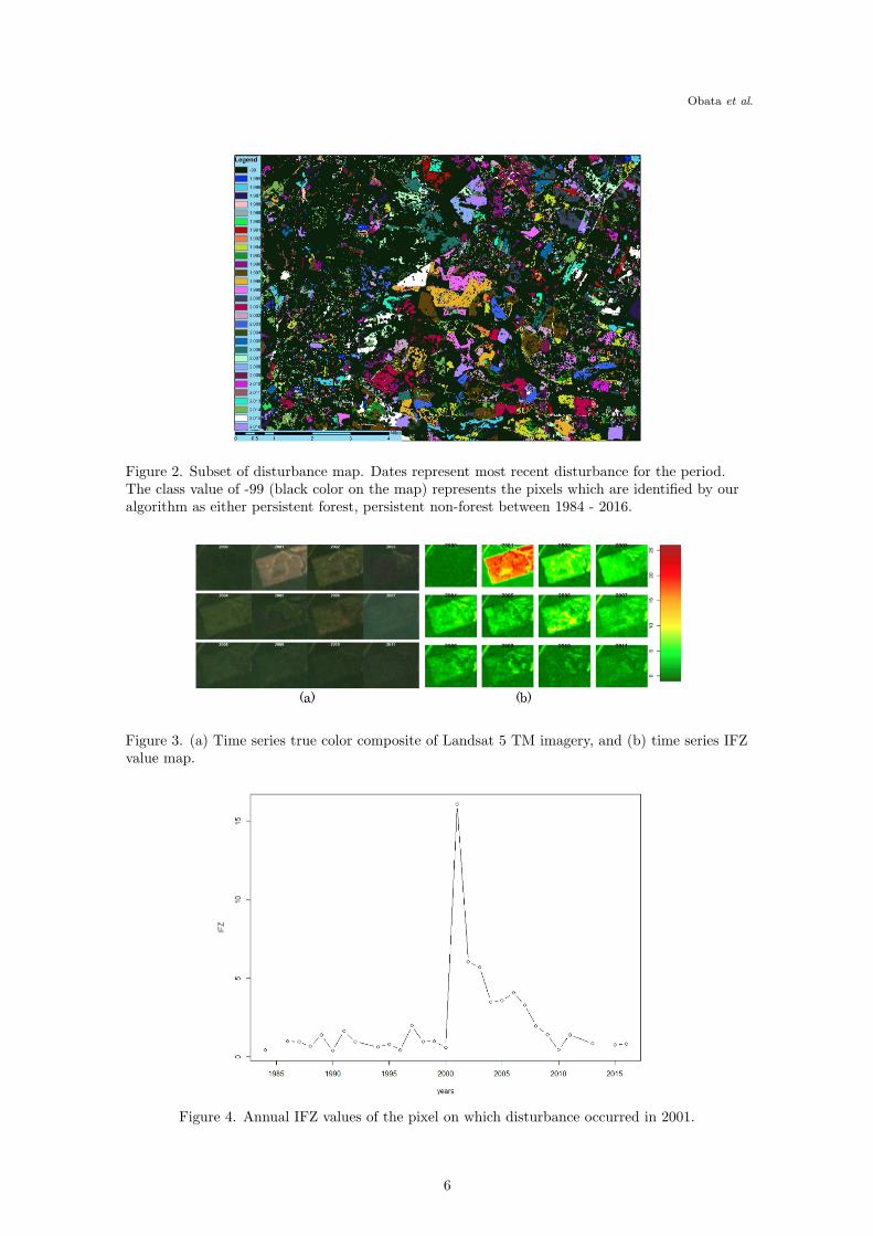
The process employed in this study produced a disturbance map (Figure 2) that illustrates theyears of the most recent major disturbances. Our assumption is that these years correlate directlywith the initiations of a new stands assuming that forestry will continue to be the designated landuse after occurrence of the major disturbance, such as final harvest and that the landowner or landmanager will begin preparation of the new forest soon after the disturbance.

A typical final harvest produces a significant change in the IFZ value, and over time, the IFZvalue will return to a range of normal values for these forests. Figure 3 illustrates through true colorcomposite (images on the left) and through IFZ value images (to the right) how the landscape wouldbe perceived when a major disturbance occurred in 2001. As time progresses and assuming forestryremains the dominant use of the land area, the imprint of the final harvest gradually diminishesin both true color and IFZ value representations. The change, or difference, that is noted betweenyears 2000 and 2001, if significant enough, would prompt the algorithm to conclude that a majordisturbance had occurred. When IFZ values for the land area are plotted over time (Figure 4), thechange in IFZ value is more dramatic between 2000 and 2001. The minor variation in IFZ valueamongst the earlier years is likely a function of local weather conditions and date of acquisition;therefore, the threshold change in IFZ amongst adjacent years (noted earlier) would have preventedthe algorithm from concluding a disturbance had occurred in other years when differences amongsubsequent years were observed.

The result of the accuracy assessment for the 3,100 reference points suggests that the overallaccuracy of the classification process was 52% (Table 1). If a ±1 year of error is allowed, therelaxed overall accuracy rises to 71%. Concerning this accuracy assessment, it is worth noting thatimagery from Google Earth generally has a higher spatial resolution than Landsat imagery. Thehistorical image tool in Google Earth automatically provides the imagery which has the highestspatial resolution of all the imagery that Google can serve. Imagery captured after 2005 has higher

5

Obata et al.

Figure 2. Subset of disturbance map. Dates represent most recent disturbance for the period.The class value of -99 (black color on the map) represents the pixels which are identified by ouralgorithm as either persistent forest, persistent non-forest between 1984 - 2016.

Figure 3. (a) Time series true color composite of Landsat 5 TM imagery, and (b) time series IFZvalue map.

Figure 4. Annual IFZ values of the pixel on which disturbance occurred in 2001.

6


spatial resolution than that of Landsat 5 TM imagery, which is 27.5 meters. Thus, Google Earthallows one to detect the subtle changes in forest character that may not be detectable with Landsat5 and 8 imagery.

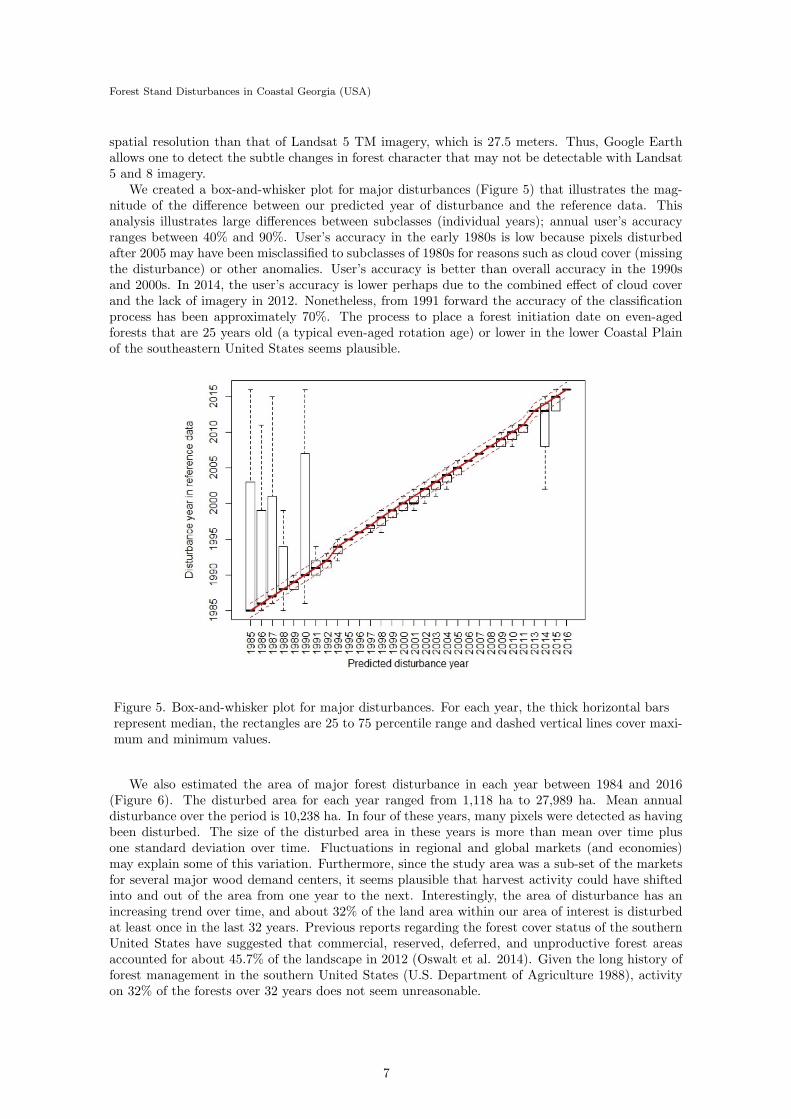
We created a box-and-whisker plot for major disturbances (Figure 5) that illustrates the mag-nitude of the difference between our predicted year of disturbance and the reference data. Thisanalysis illustrates large differences between subclasses (individual years); annual user’s accuracyranges between 40% and 90%. User’s accuracy in the early 1980s is low because pixels disturbedafter 2005 may have been misclassified to subclasses of 1980s for reasons such as cloud cover (missingthe disturbance) or other anomalies. User’s accuracy is better than overall accuracy in the 1990sand 2000s. In 2014, the user’s accuracy is lower perhaps due to the combined effect of cloud coverand the lack of imagery in 2012. Nonetheless, from 1991 forward the accuracy of the classificationprocess has been approximately 70%. The process to place a forest initiation date on even-agedforests that are 25 years old (a typical even-aged rotation age) or lower in the lower Coastal Plainof the southeastern United States seems plausible.

Figure 5. Box-and-whisker plot for major disturbances. For each year, the thick horizontal barsrepresent median, the rectangles are 25 to 75 percentile range and dashed vertical lines cover maxi-mum and minimum values.

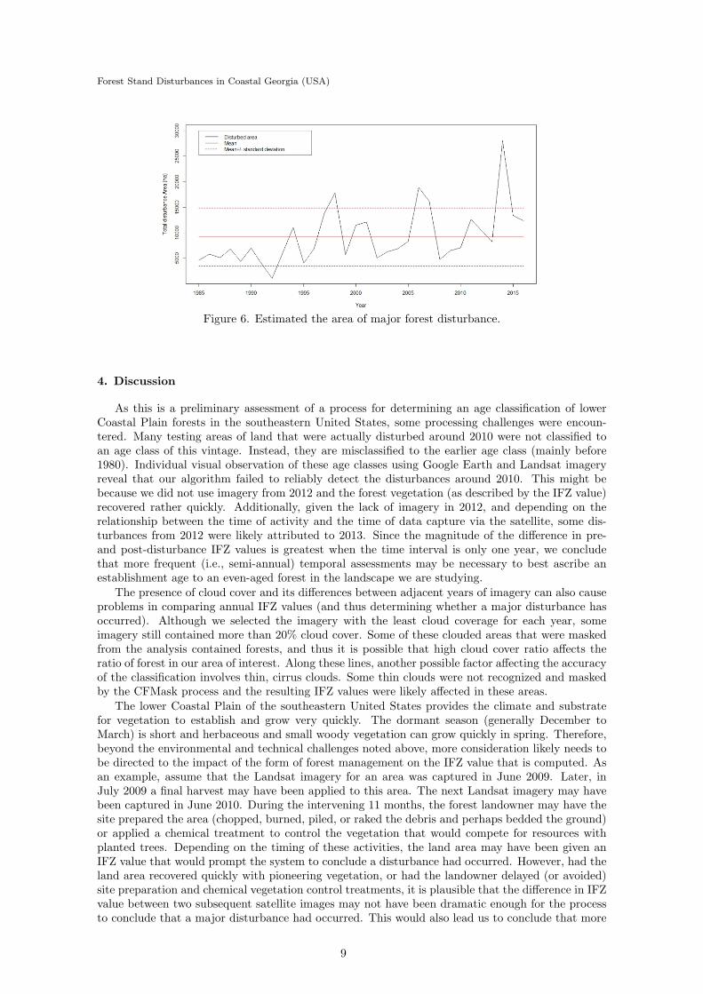
We also estimated the area of major forest disturbance in each year between 1984 and 2016(Figure 6). The disturbed area for each year ranged from 1,118 ha to 27,989 ha. Mean annualdisturbance over the period is 10,238 ha. In four of these years, many pixels were detected as havingbeen disturbed. The size of the disturbed area in these years is more than mean over time plusone standard deviation over time. Fluctuations in regional and global markets (and economies)may explain some of this variation. Furthermore, since the study area was a sub-set of the marketsfor several major wood demand centers, it seems plausible that harvest activity could have shiftedinto and out of the area from one year to the next. Interestingly, the area of disturbance has anincreasing trend over time, and about 32% of the land area within our area of interest is disturbedat least once in the last 32 years. Previous reports regarding the forest cover status of the southernUnited States have suggested that commercial, reserved, deferred, and unproductive forest areasaccounted for about 45.7% of the landscape in 2012 (Oswalt et al. 2014). Given the long history offorest management in the southern United States (U.S. Department of Agriculture 1988), activityon 32% of the forests over 32 years does not seem unreasonable.

7

Obata et al.

Tab

le1.

Error

matrixof

accu

racy

assessment.

Reference

-99

1985

1986

1987

1988

1989

1990

1991

1992

1994

1995

1996

1997

1998

1999

2000

2001

2002

2003

2004

2005

2006

2007

2008

2009

2010

2011

2013

2014

2015

2016

RT

UA

RUA

Projection

-99

682

11

21

11

21

13

31

21

12

21

12

100

68%

68%

1985

2539

94

12

11

21

21

81

12

100

39%

48%

1986

1812

329

42

21

32

23

24

11

2100

32%

53%

1987

812

504

11

12

13

32

64

2100

50%

66%

1988

211

1342

31

12

11

13

61

12

100

42%

55%

1989

1231

361

21

22

11

11

23

31

100

36%

68%

1990

281

24

231

53

11

11

11

13

45

23

100

31%

38%

1991

525

444

31

11

11

11

11

41

5100

44%

73%

1992

1427

424

11

11

13

21

2100

42%

73%

1994

161

11

701

13

11

13

100

70%

72%

1995

61

11

575

11

14

4100

75%

81%

1996

131

32

711

11

11

31

1100

71%

74%

1997

132

2050

22

11

21

6100

50%

72%

1998

232

12

11

1837

51

21

11

11

11

100

37%

60%

1999

61

11

2762

11

100

62%

89%

2000

151

21

123

431

11

11

42

12

100

43%

67%

2001

181

145

322

1100

32%

79%

2002

163

2448

22

21

11

100

48%

74%

2003

181

13

2247

11

11

12

1100

47%

70%

2004

131

141

381

11

12

100

38%

80%

2005

121

3147

21

14

1100

47%

80%

2006

201

21

110

552

11

41

1100

55%

67%

2007

271

11

11

34

556

100

55%

65%

2008

52

11

15

766

11

1100

76%

87%

2009

61

11

11

21

124

583

100

58%

85%

2010

41

12

11

118

701

100

70%

89%

2011

181

11

21

12

2249

2100

49%

73%

2013

110

881

100

88%

99%

2014

281

11

21

11

22

11

32

42

112

331

100

33%

46%

2015

181

11

21

45

12

13

1047

299

47%

60%

2016

62

13

14

21

674

100

74%

80%

CT

501

5562

9187

4471

8654

100

91102

7480

101

115

7483

9680

7176

66123

100

116

79164

7474

109

3099

PA

14%

71%

52%

55%

48%

82%

44%

51%

78%

70%

82%

70%

68%

46%

61%

37%

43%

58%

49%

48%

66%

72%

83%

62%

58%

60%

62%

54%

45%

64%

68%

52%

RPA

14%

93%

85%

79%

89%

86%

80%

88%

87%

79%

86%

90%

93%

82%

89%

77%

77%

87%

94%

88%

82%

80%

94%

86%

82%

82%

76%

62%

59%

73%

70%

71%

RT:Row

total,UA:User’saccuracy,RUA:Relaxed

User’saccuracy,CT:Columntotal,PA:Producer’saccuracy,RPA:Relaxed

Producer’saccuracy.

8


Figure 6. Estimated the area of major forest disturbance.

4. Discussion

As this is a preliminary assessment of a process for determining an age classification of lowerCoastal Plain forests in the southeastern United States, some processing challenges were encoun-tered. Many testing areas of land that were actually disturbed around 2010 were not classified toan age class of this vintage. Instead, they are misclassified to the earlier age class (mainly before1980). Individual visual observation of these age classes using Google Earth and Landsat imageryreveal that our algorithm failed to reliably detect the disturbances around 2010. This might bebecause we did not use imagery from 2012 and the forest vegetation (as described by the IFZ value)recovered rather quickly. Additionally, given the lack of imagery in 2012, and depending on therelationship between the time of activity and the time of data capture via the satellite, some dis-turbances from 2012 were likely attributed to 2013. Since the magnitude of the difference in pre-and post-disturbance IFZ values is greatest when the time interval is only one year, we concludethat more frequent (i.e., semi-annual) temporal assessments may be necessary to best ascribe anestablishment age to an even-aged forest in the landscape we are studying.

The presence of cloud cover and its differences between adjacent years of imagery can also causeproblems in comparing annual IFZ values (and thus determining whether a major disturbance hasoccurred). Although we selected the imagery with the least cloud coverage for each year, someimagery still contained more than 20% cloud cover. Some of these clouded areas that were maskedfrom the analysis contained forests, and thus it is possible that high cloud cover ratio affects theratio of forest in our area of interest. Along these lines, another possible factor affecting the accuracyof the classification involves thin, cirrus clouds. Some thin clouds were not recognized and maskedby the CFMask process and the resulting IFZ values were likely affected in these areas.

The lower Coastal Plain of the southeastern United States provides the climate and substratefor vegetation to establish and grow very quickly. The dormant season (generally December toMarch) is short and herbaceous and small woody vegetation can grow quickly in spring. Therefore,beyond the environmental and technical challenges noted above, more consideration likely needs tobe directed to the impact of the form of forest management on the IFZ value that is computed. Asan example, assume that the Landsat imagery for an area was captured in June 2009. Later, inJuly 2009 a final harvest may have been applied to this area. The next Landsat imagery may havebeen captured in June 2010. During the intervening 11 months, the forest landowner may have thesite prepared the area (chopped, burned, piled, or raked the debris and perhaps bedded the ground)or applied a chemical treatment to control the vegetation that would compete for resources withplanted trees. Depending on the timing of these activities, the land area may have been given anIFZ value that would prompt the system to conclude a disturbance had occurred. However, had theland area recovered quickly with pioneering vegetation, or had the landowner delayed (or avoided)site preparation and chemical vegetation control treatments, it is plausible that the difference in IFZvalue between two subsequent satellite images may not have been dramatic enough for the processto conclude that a major disturbance had occurred. This would also lead us to conclude that more

9

Obata et al.

frequent (i.e., semi-annual) temporal assessments may be necessary to best ascribe an establishmentage to an even-aged forest in the landscape we are studying.

4. Conclusions

The algorithm presented here, which is similar to the Vegetation Change Tracker and othermethods for automatic detection of changes in land use, was developed to help understand the ageclass distribution of current forests in the lower Coastal Plain of the State of Georgia (USA). Thealgorithm relied on three bands (visible and infrared regions) within Landsat data and a long timeseries of growing season images to determine when major forest disturbance events occurred. It wasmoderately successful in determining the years of disturbances and current age classes of forestsin this region, given that many of them are managed as even-aged stands. The development andits testing met some technological challenges. The lack of suitable imagery for two years requiredmodifications to the mathematical assessment of the integrated forest Z score (IFZ value), andthe presence of cloud cover, ubiquitous to the area during the growing season, may have led tosome classification errors. More specifically, cloud cover, when masked from the analysis, couldhave required examining non-adjacent years for evidence of disturbance, which may have added toclassification error.

Acknowledgement

This graduate research is funded by Japan Student Service Organization. This work was alsosupported by the U.S. Department of Agriculture, National Institute of Food and Agriculture,McIntire-Stennis project 1012166, administered by the University of Georgia. We thank our col-leagues from the University of Georgia Warnell School of Forestry and Natural Resources whoprovided valuable advice and expertise that greatly assisted the research.

References

Bettinger, P., Boston, K., Siry, J.P., Grebner, D.L. (2017) Forest Management and Planning, 2ndedition. Academic Press, New York.

Brooks, E.B., Wynne, R.H., Thomas, V.A., Blinn, C.E., Coulston, J.W. (2014) On-the-fly massivelymultitemporal change detection using statistical quality control charts and Landsat data, IEEET, Geosci. Remote. 52: 3316–3332.

Cieszewski, C.J., Zasada, M., Borders, B.E., Lowe, R.C., Zawadzki, J., Clutter M.L., Daniels R.F.(2004) Spatially explicit sustainability analysis of long-term fiber supply in Georgia, USA, ForestEcol. Manag. 187(2-3): 349–359.

Cieszewski, C.J., Liu, S., Lowe, R.C., Zasada M. (2011) Spatially explicit biomass supply sustain-ability analysis for bioenergy mill siting in Georgia, USA, The Open Forest Sci. J. 4: 2–14.

Chen, J., Zhu, X., Vogelmann, J.E., Gao, F., Jin, S. (2011) A simple and effective method for fillinggaps in Landsat ETM+ SLC-off images, Remote Sens. Environ. 115: 1053–1064.

Georgia Forestry Commission (2018) Conservation Reserve Program (CRP), <http://www.gfc.state.ga.us/forest-management/private-forest-management/landowner-programs/other-landowner-programs/> (Accessed 12 February 2018).

Goward, S.N., Huang, C., Zhao, F., Schleeweis, K., Rishmawi, K., Lindsey, M., Dungan, J.L.,Michaelis, A. (2015) NACP NAFD project: Forest disturbance history from Landsat, 1986-2010,ORNL DAAC, Oak Ridge, TN.

Huang, C., Goward, S.N., Schleeweis, K., Thomas, N., Masek, J.G., Zhu, Z. (2009) Dynamics ofnational forests assessed using the Landsat record: Case studies in eastern United States, RemoteSens. Environ. 113: 1430–1442.

10


Huang, C., Goward, S.N., Masek, J.G., Thomas, N., Zhu, Z., Vogelmann, J.E. (2010) An automatedapproach for reconstructing recent forest disturbance history using dense Landsat time seriesstacks, Remote Sens. Environ. 114: 183–198.

Jin, S., Yang, L., Danielson, P., Homer, C., Fry, J., Xian, G. (2013) A comprehensive changedetection method for updating the National Land Cover Database to circa 2011, Remote Sens.Environ. 132: 159–175.

Kennedy, R.E., Yang, Z., Cohen, W.B. (2010) Detecting trends in forest disturbance and recoveryusing yearly Landsat time series: 1. LandTrendr – Temporal segmentation algorithms, RemoteSens. Environ. 114: 2897–2910.

Liu, S., Cieszewski, C. (2009) Impacts of management intensity and harvesting practices on long-term forest resource sustainability in Georgia, Math. Comput. Forestry Nat.-Res. Sci. 1(2):52–66.

Obata, S. (2018) Estimation of forest stand disturbance through implementation of vegetationchange tracker algorithm using Landsat time series stacked imagery in coastal Georgia, Math.Comput. Forestry Nat.-Res. Sci. 10(1): 32.

Oswalt, S.N., Smith, W.B., Miles, P.D., Pugh, S.A. (2014) Forest resources of the United States,2012: A technical document supporting the Forest Service update of the 2010 RPA Assessment,USDA Forest Service, Washington, D.C. General Technical Report WO-91.

Roy, D.P., Wulder, M.A., Loveland, T.R., Woodcock, C.E., Allen, R.G., Anderson, M.C., ..., Scam-bos, T.A. (2014) Landsat-8: Science and product vision for terrestrial global change research,Remote Sens. Environ. 145: 154–172.

U.S. Department of Agriculture (1988) The South’s Fourth Forest: Alternatives for the Future,USDA Forest Service, Washington, D.C. Forest Resource Report No. 24.

U.S. Geological Survey (2017) EarthExplorer, <https://earthexplorer.usgs.gov/> (Accessed 21 June2017).

Vogelmann, J.E., Xian, G., Homer, C., Tolk, B. (2012) Monitoring gradual ecosystem change usingLandsat time series analyses: Case studies in selected forest and rangeland ecosystems, RemoteSens. Environ. 122: 92–105.

Zhu, Z., Woodcock, C.E., Holden, C., Yang, Z. (2015) Generating synthetic Landsat images basedon all available Landsat data: Predicting Landsat surface reflectance at any given time, RemoteSens. Environ. 162: 67–83.

11

preliminary analysis of forest stand disturbances in

Documents