Preliminary Design of an 18MVA Industrial

System A Major Qualifying Project submitted to the faculty of

WORCESTER POLYTECHNIC INSTITUTE

In partial fulfillment of the requirements for the

Degree of Bachelor of Science

An MQP by:

Alex Legere, amlegere@wpi.edu

Submitted to:

Professor Alexander Emanuel, ECE

Submitted on:

4/24/2018

This Major Qualifying Project is submitted in partial fulfillment of the degree requirements of

Worcester Polytechnic Institute. The views and opinions expressed herein are those of the author

and do not necessarily reflect the positions or opinions of Worcester Polytechnic Institute.

Abstract

The purpose of this project was to explore power factor correction in an industrial setting.

A theoretical factory is looking to expand its operation. In order to do so, they are opening up a

new wing in the factory. In designing the new wing, they need to supply power to the lights and

to the various induction motors required to run the machinery. These motors operate with a

certain power factor. They manufacturer wants to correct this lower-than-desired power factor so

that the motors draw less current, ultimately decreasing losses in conductors and saving them

money on their operation.

Acknowledgements

I would like to thank my advisor Professor Emanuel for taking me under his wing when I

desperately needed another project, for his guidance and encouragement along the way, and for

his patience at times when the project may not have been going as smoothly as we would have

liked. Without him, this project would not have been possible.

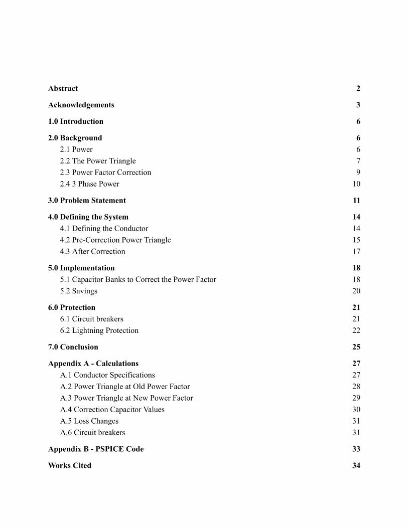
Abstract 2

Acknowledgements 3

1.0 Introduction 6

2.0 Background 6 2.1 Power 6 2.2 The Power Triangle 7 2.3 Power Factor Correction 9 2.4 3 Phase Power 10

3.0 Problem Statement 11

4.0 Defining the System 14 4.1 Defining the Conductor 14 4.2 Pre-Correction Power Triangle 15 4.3 After Correction 17

5.0 Implementation 18 5.1 Capacitor Banks to Correct the Power Factor 18 5.2 Savings 20

6.0 Protection 21 6.1 Circuit breakers 21 6.2 Lightning Protection 22

7.0 Conclusion 25

Appendix A - Calculations 27 A.1 Conductor Specifications 27 A.2 Power Triangle at Old Power Factor 28 A.3 Power Triangle at New Power Factor 29 A.4 Correction Capacitor Values 30 A.5 Loss Changes 31 A.6 Circuit breakers 31

Appendix B - PSPICE Code 33

Works Cited 34

Table of Figures

Figure 1 7

Figure 2 8

Figure 3 9

Figure 4 10

Figure 5 12

Figure 6 14

Figure 7 17

Figure 8 18

Figure 9 21

Figure 10 21

Figure 11 22

Figure 12 22

Figure 13 23

Figure 14 23

Figure 15 24

1.0 Introduction

Especially in an industrial setting, efficiency is key. It can mean the difference between

facing heavy fines and meeting government standards, between being on budget versus being

over budget, between on time and past the deadline. An inefficient factory will face problems

with costs that could force them to close. One way to reduce inefficiencies in their system and

reduce costs, at least for power, is through power factor correction.

Power factor is essentially a measure of how much of the power consumed is actually

useable by the equipment. The factory is drawing drawing current for all the power consumed,

not just what is used by the equipment. By correcting this power factor, you keep the power

actually used by the equipment the same, but decrease the total consumed, reducing the current

necessary to get the power to the equipment. In doing so, you decrease the losses in the

transmission system and reduce the costs of building because you can build to a lower current.

2.0 Background

2.1 Power

Power is a measure of energy consumed over time. Generally measured in Watts, it

represents Joules per second. Power can be mechanical, it can be magnetic, or it can be electric.

Motors, for example, convert electric power into mechanical power plus heat losses, such that

Figure 1 is an accurate representation of the input and output powers of a motor.

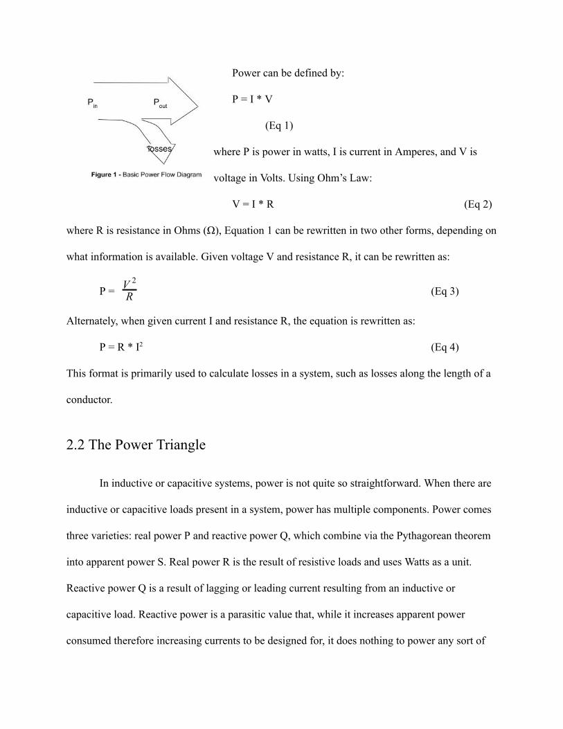
Power can be defined by:

P = I * V

(Eq 1)

where P is power in watts, I is current in Amperes, and V is

voltage in Volts. Using Ohm’s Law:

V = I * R (Eq 2)

where R is resistance in Ohms (Ω), Equation 1 can be rewritten in two other forms, depending on

what information is available. Given voltage V and resistance R, it can be rewritten as:

P = RV 2

(Eq 3)

Alternately, when given current I and resistance R, the equation is rewritten as:

P = R * I 2 (Eq 4)

This format is primarily used to calculate losses in a system, such as losses along the length of a

conductor.

2.2 The Power Triangle

In inductive or capacitive systems, power is not quite so straightforward. When there are

inductive or capacitive loads present in a system, power has multiple components. Power comes

three varieties: real power P and reactive power Q, which combine via the Pythagorean theorem

into apparent power S. Real power R is the result of resistive loads and uses Watts as a unit.

Reactive power Q is a result of lagging or leading current resulting from an inductive or

capacitive load. Reactive power is a parasitic value that, while it increases apparent power

consumed therefore increasing currents to be designed for, it does nothing to power any sort of

machinery or electronics on the system.

Capacitors result in a current waveform that

“leads” the voltage waveform, meaning that

the current waveform is out of phase with

the voltage waveform, being ahead by some

angle as in Figure 2a . Inductors result in a “lagging” current waveform, meaning the current

waveform is some angle behind the voltage waveform, as seen in Figure 2b . In a system with

capacitors, inductors, and resistors, the net lag or lead in the system can be modeled as a literal

triangle, aka the Power Triangle, as seen in Figure 2c . The angle φ in the triangle is the same the

angle by which the current lags or leads the voltage. By taking cos(φ), a relationship between P,

Q, and S is formed called the “Power Factor”. The Power Factor is essentially a measure of how

much of that power is usable, i.e. real power, relative to the apparent power S that gets consumed

by the system.

2.3 Power Factor Correction

In order to decrease the value of Q and correct the power factor, an additional inductive

or capacitive load is needed. If the original power factor is due to an inductive loads, the power

factor can be corrected with the proper capacitance. If the power factor is due to a capacitive

load, it can be corrected using the correct size inductor.

The use of inductive loads to correct capacitive loads, and vice versa, is due to the

lagging of the current in inductive loads and the leading of current in capacitive loads. If the

current is lagging, it can be corrected by adding a capacitive load, cancelling out the lag in the

current waveform by adding a lead, in a sense. The same happens when an inductor is used to

correct a leading current waveform from a capacitor.

An alternate explanation comes from drawing them as arrows. Figure 3 shows the

current and voltages. Figure 3a shows what happens when

the power factor is 1, or “unity”, meaning there is no phase

shift in the current waveform. Figure 3b shows a capacitive

load. Figure 3c shows an inductive load. Note that one is

pointing up, and the other is pointing down. This shows that

inductors can be used to correct a capacitive load’s power

factor, and that capacitors can be used to correct an inductive

load’s power factor.

In order to correct the power factor, the capacitances and inductances need to be the

correct size. They must match so that the reactive power through each is equal and opposite to

the original reactive power (assuming a correction to unity, or to a power factor of 1). In order to

find the value of a capacitor given an inductive load, use the equation:

C = Q2πf V*

2LL

(Eq 5)

where Q is the reactive power, f is the frequency (typically 60 Hz in power systems), and V LL is

the line-to-line voltage. Likewise, if the load is capacitive, and the the value of a corrective

inductor is needed, use the equation:

L = V 2LL

2πf Q*(Eq 6)

Equations 5 and 6 are the necessary equations to calculate the capacitance and inductance needed

to correct inductive and capacitive power factors respectively. All that is needed is the

uncorrected power factor.

2.4 3 Phase Power

Power is often delivered as what is called “Three Phase Power”. Three Phase Power is

power delivered as three separate current waveforms of equal magnitude, each 120° out of phase

from each other. This ensures that there is constant power

delivery, rather than the on-and-off delivery from single

phase. The Three Phase current waveforms can be seen

in Figure 4 .

Notation in Three Phase Power is less straightforward

that in single phase. The three phases are labelled I a , I b ,

and I c . These correspond to voltages V a , V b , and V c . However, whenever voltages are needed for

calculations, they are measured in V LL and V LN . V LL is voltage line-to-line. This is the voltage of

the phases relative to each other. Likewise, V LN stands for voltage line-to-neutral, or the voltage

of one line relative to the neutral wire. The conversion process is quite simple:

V LN = V LL /√3 (Eq 7)

This equation is used quite frequently, so it is an important one to memorize.

One last important thing to note is that in calculations involving three phase systems, it is

often the case that equations must take into account that there are multiple lines involved, so

there needs to be a scaling factor of 3. One such notable equation is calculating line losses, such

that equation 4 is changed to:

P = 3 * R * I 2 (Eq 8)

The new coefficient of 3 is because there are three lines, and therefore three times the resistance.

3.0 Problem Statement

A theoretical factory is looking to expand their production a bit by opening a new wing of

the factory. The new wing requires power for lights and for induction motors that will run the

machines necessary for production. The wing of the factory is supplied by a 3-phase voltage of

14kV RMS, line-to-line at 60 Hz. It runs into a step-down transformer that steps it down to 440

V RMS, line-to-line. Out of that transformer, it runs along a line for 50 meters before it splits

into two branches: one running to the factory’s induction motors, and one running to the lights.

The entire system can be seen in Figure 5 .

The induction motors run on 440 V RMS , with an efficiency of 90%, and an inductive

power factor of 85%. The max power drawn by the motors is 18 MVA, but the load varies in

time. It follows a sine wave that runs from 60% load to 100% load (10.8 MVA to 18 MVA) over

the period of 24 hours. The lights draw 0.5 MVA, and have a total harmonic distortion of 28%.

The goal of the project is to correct the power factor of the induction motors to 98%. In

order to do this, one must calculate and determine:

● The size of the Circuit Breakers and Fuses

● Transformer ratings

● Capacitors needed to correct the power factor

● Conductor size and material

● Surge and overload protection

● Power lost

4.0 Defining the System

All calculations are compiled for easy checking in Appendix A.

4.1 Defining the Conductor

In order to determine the details of the conductor, the current out of the transformer

secondary must be found. Given a total of 18.5 MVA that needs to be carried to the lights and to

the motors, and given a voltage of 440 V LL , or 254 V LN , the total current carried by the 50 meter

conductor running from transformer outside all the way to the new wing of the factory is:

I = = 24278 A S3 V * LN

= 3 254 V*18.5x10 V A6

(Eq 9)

This is the maximum current to run through each of the conductors, which is the bar minimum

that they musteach be able to bear. Note the 3 in the denominator, meaning the power needs to be

divided amongst the three conductors of the system. In order to find the necessary cross-sectional

area, both the current and current density are needed. The equation for current Density (J) is:

J = I / A (Eq 10)

where A is the cross-sectional area. The given minimum current density is 3 A/mm 2 , i.e. J ≥ 3

A/mm 2 . Using this value and rearranging Equation 10, the cross-sectional area can be found:

A = = 8093 mm 2 IJ = 24278 A

3 A mm/ 2

Bear in mind, this cross-sectional area is meant to be the area of only one single conductor, all of

which should be the same size. To make for easier routing throughout the facility, a rectangular

cross-section would be ideal for the conductor, as it could be made thinner along one axis, and

therefore easier to bend whenever necessary. A good idea for the dimensions may be something

along the lines of 130 x 62 mm, making it not too thin in any one direction, but not so thick it

would be impossible to bend and route throughout the building. Compare this value to a diameter

of roughly 100 mm should a circular conductor be chosen. It would make it significantly more

difficult to route this conductor throughout the facility.

The wire, as with all materials, would have some level of resistance along its length. The

equation for resistance along the length of a conductor is:

R = ρ lA

(Eq 11)

The length l is given as 50 meters, and the cross-sectional area A was found to be 8093 mm 2 , or

0.008903 m 2 , so all that is needed is ⍴, or the resistivity of whatever material is chosen for the

conductor. A common material for the conductor is copper, which has a resistivity ρ Cu of

1.72x10 -8 Ω*m. Given this material’s resistivity and equation 11, the resistance is:

R = = 1.06x10 -4 Ω.72x10 Ω 1 8−* m * 50 m

0.008903 m2

Lastly, given this resistance, the losses along the conductor can be calculated. In a three phase

system, the losses along the conductor can be calculated using a variation of equation 4 which,

similar to equation 9, takes into account that there are three separate but identical conductors.

The equation for losses along the three conductors is:

P = 3 * I 2 * R

Given the calculated current of 24278 A and resistance of 1.06x10 -4 Ω, the losses along the

conductor are:

P = 3 * (24278 A) 2 * 1.06x10 -4 Ω = 187436 W

In summary, the conductor creates huge losses in the uncorrected system. Unfortunately, the

conductor dimensions must remain the same after correcting the power factor.

4.2 Pre-Correction Power Triangle

Given the graph of the level of operation

throughout the day in Figure 6 , the maximum

power draw of the motors is 18 MVA. The

original power factor for these motors is also

given as 0.85. Using these values, the sides of the

power triangle (S, P, Q) can be calculated for

various times throughout the day. In order to

correct the power factor of the system, the

original S, P and Q must be known at multiple times throughout the day, otherwise the power

factor may only be corrected for one single point in the day, which wouldn’t make much sense.

For simplicity of calculation, the percentages are chosen at the daily minimum capacity the daily

average capacity, and the daily maximum capacity, or 60%, 80% and 100% respectively.

At the maximum capacity, it is given that the apparent power S max = 18 MVA. In order to

find the real power, 2 of 3 values must be known: S, Power Factor (PF), and Q. S and PF are

known, so the equation:

P = S * PF (Eq 12)

is usable. Given S max = 18 MVA and PF = 0.85, equation 12 yields the result:

P max = 18 MVA * 0.85 = 15.3 MW

Which is what drives the motors at their peak levels of operation. This value will stay here even

after correcting the power factor, otherwise the motors would not function at the levels necessary

for peak operations. Lastly, the value that will be corrected, Q, must be calculated. This can be

found simply using the Pythagorean theorem, as it is the last leg of the power triangle, which is a

right triangle. The equation to find it given P and S is:

Q = √S2 − P 2 (Eq 13)

Knowing S max and P max , Q max can be found as:

Q max = = 9.5 MVar √18 15.32 − 2

Q max is the maximum value that will be corrected.

At the average operation levels for the motors, or at 80%, the apparent power S ave = 14.4

MVA. Given the power factor of 0.85 and equation 12, the real power P ave can be found as:

P ave = 0.85 * 14.4 MVA = 12.24 MW

Which will remain after correction. Lastly, the reactive power is:

Q ave = = 7.6 MVar √14.42 − 12.242

Again, this is the value to be corrected.

Lastly, the motors will be operating at 60% at the bare minimum, such as in the middle of

the night. This means that the apparent power S min = 10.8 MVA. Given this and equation 12:

P min = 0.85 * 10.8 MVA = 9.18 MW

Yet again, this value will remain the same after correction. Lastly, given S min and P min :

Q min = = 5.7 MVar √10.82 − 9.182

Just a reminder that these values are before power factor correction.

4.3 After Correction

The desired corrected power factor is 0.98. The induction motors at 100%, 80%, and 60%

require the input of real power P of 15.3, 12.24, and 9.18 MW respectively. Given the power P

and the new power factor, the equation to find the new apparent power S is a variation of

equation 12:

S = P/PF (Eq 14)

Once S is found, the equation to find Q stays the same as in Equation 13.

At max, the new S is:

S max = 15.3 / 0.98 = 15.6 MVA

Note how much closer the new value to the real power. This means Q max is expected to be much

smaller. Now, applying equation 13:

Q max = = 3 MVar √15.62 − 15.32

At the average of 80%, the real power P ave is a constant 12.24 MW. Applying equation 14

again yields:

S ave = 12.24 / 0.98 = 12.5 MVA

Again, not too much larger than P ave , so Q ave can be expected to be even smaller. Applying

equation 13 again yields:

Q ave = = 2.5 MVar √12.52 − 12.242

Lastly, at the minimum operation level of 60%, the real power P min is 9.18 MW. Applying

equation 14 one last time, the apparent power at the minimum is:

S min = 9.18 / 0.98 = 9.36 MVA

That, like the last two times, shows that Q min can be expected to be even smaller. Applying

equation 13 one final time yields:

Q min = = 1.8 MVar √9.362 − 9.182

At all these levels, the apparent and reactive power are significantly smaller than before. This

will, in the long run, save the facility lots of money on power costs, and less of a burden on the

system means less maintenance costs.

5.0 Implementation

5.1 Capacitor Banks to Correct the Power Factor

The motors in the facility are inductive motors. This means that the power factor and the

reactive powers are all inductive, and require the use of capacitors in order to correct them. In

order to determine the proper capacitor size, the difference in the reactive power at each level

must be known. The values are shown in Table 1 to compare them at the old and new power

factor, as well as the difference between the two.

Table 1 - Reactive Powers and Corresponding Capacitances

% Q Old (MVar)

Q New (MVar)

ΔQ = Q Old -Q New (MVar)

Total Capacitance

Capacitance for Step

100% 9.5 3 6.5 89 mF 17.8 mF

80% 7.6 2.5 5.1 71.2 mF 17.8 mF

60% 5.7 1.8 3.9 53.4 mF 53.4 mF

Using the ΔQ values from Table 1 , it is possible to know what correction

capacitors to use based on the desired change

change in Q. In order to correct the power factor at

all the chosen points throughout the day, one single

capacitor is not enough, otherwise the power factor

will be corrected only at that point in the day. As

the level of operation increases, so does the change

in Q, and therefore so does the capacitance needed.

As such, a possible implementation is a capacitor

bank, as seen in Figure 7 . This capacitor bank contains however many capacitors needed for

however many points were chosen. In this case,

three capacitors were chosen because only three

levels were chosen. The capacitors are connected

in parallel, with switches on all but the base

capacitor, the minimum capacitance, which

corresponds to 60% capacity, the lowest the

motors go over the course of the day. The other

capacitors are each in series with their own

switch, such that they are switched on around the time

when the system typically reaches that point. They are in parallel because capacitors in parallel

add due to capacitance being a function of the surface area between the plates of a capacitor, and

putting them in parallel effectively adds the surface areas. These capacitor banks are

implemented in parallel to the motor, with one on each phase, as seen in Figure 8 .

In order to find the size of the total capacitances at each level, equation 5 is used, subbing

in ΔQ for Q, so that the desired Q is reached. At max, the total capacitance is:

C max = = 89 mF6.5x10 MV ar6

2π 60 Hz 440V* *2

At the average:

C ave = = 71.2 mF6.5x10 MV ar6

2π 60 Hz 440V* *2

And the minimum:

C min = = 53.4 mF6.5x10 MV ar6

2π 60 Hz 440V* *2

These capacitances, as mentioned, are the total capacitances need to correct the power factor at

the given points, assuming a frequency of 60 Hz (f = 60 Hz) and a line-to-line voltage of 440 V

(V LL = 440 V). However, the actual values of capacitances need to be found. This is simply done

by subtracting them from one another, such that:

C 1 = C min = 53.4 mF

C 2 = C ave - C min = 71.2 - 53.4 = 17.8 mF

C 3 = C max - C ave = 89 - 71.2 = 17.8 mF

These are the values of the capacitors in each capacitor bank. Again, these values assume 60 Hz

and 440 Volts line-to-line. Should neither of those be the case, these capacitor values would be

wrong.

5.2 Savings

With the new power factor and new Q and S values, various things change. Most notably

is the current draw on the conductor from before is lower. The length, resistance, and

cross-sectional area remain the same because not only would that incur significant installation

costs, but it would spell disaster for the system should the capacitor banks fail. Given the new

new maximum apparent power for the motors of 15.6 MVA, and the unchanged apparent power

draw of the lights being 0.5 MVA, the total apparent power carried by the conductor is 16.1

MVA. In order to calculate the reduction in losses, using equation 9, the maximum current

carried by the conductor is:

I = = 21128 A3 254V*16.1x10 V A6

This reduction in current leads to fewer losses from the conductor’s resistance. Given that it stays

the same (due to the dimensions and the resistivity of the material remaining constant) at a value

of 1.06x10 -4 Ω, using equation 8, which was losses in a three phase system:

P = 3 * (21128 A) 2 * 1.06x10 -4 Ω = 141953 W = 141.953 kW

Remember that the losses before the power factor correction were 187.44 kW. That

means that the power saved, the difference between the two values, is:

ΔP = P old - P new = 187436 - 141953 = 45483 Watts = 45.5 kW

Using the power saved from losses alone, the money saved from losses alone can now be

determined. Given a price tag of $0.14 per kiloWatt-hour (Cost = 0.14 $/kWh), the money saved

is:

Savings/day = ΔP * time * Cost = 45.5 kW * 24h/day * $0.14/kWh = $152.81/day

Assuming the motors were running at their maximum all day, the facility would save $152.81

every day just from losses in the conductor.

6.0 Protection

6.1 Circuit breakers

One simple way to protect against excessive currents, translating to overvoltage

protection thanks to Ohm’s law, is through the use of basic circuit breakers. For simplicity’s sake,

a good possible choice for circuit breaker size is 125% of the maximum possible current in that

wire. In the 50 meter long conductor, the maximum possible current is roughly 24278 A. The

circuit breaker that is roughly 125% the maximum possible current there is 30 kA.

On the primary of the initial transformer, the 14000 V:440 V step down transformer, the

current is found with an equivalency given in equation 15:

V 2

V 1 = I1

I2 (Eq 15)

This equivalence can be used to find the current on the primary side of the transformer. That

current is:

I 1 = = = 763 AmpsV 1

I V2 * 214000V

24278A 440V*

Given this current, a circuit breaker placed before the transformer should have a value of 953

Amps.

The transformer leading to the lights is a 440V:120V step down transformer, because

lights typically run on 120 Volts RMS. Given that the lights consume 0.5 MVA, applying a

rearrangement of equation 1 gives the current on both the secondary and the primary. On the

primary side, along side a scaling factor of 3 to account for the three phases, the current is:

I = = 379 A S3 V*

= 3 440*0.5x106

This current means a circuit breaker on the primary of the lights’ transformer would need to be

rated for 473 A. Meanwhile, the current on the secondary, where the voltage is 120 V:

I = = 1.39 kA S3 V*

= 3 120*0.5x106

The required circuit breaker would need to be rated for 1740 A.

Lastly, the current flowing the conductor directly to the motors needs to be calculated.

Given the main conductor’s current of 24278 A, the current into the lights’ transformer primary

of 379 A, and Kirchoff’s Current Law (total current into a node equals total current out of the

node), the current running in that wire is:

I motor = I conductor - I lights = 24278 - 379 = 23899 A

That means the circuit breaker in that section needs to be rated for 29.9 kA. It is important to

note that, much like nearly everything in the calculations, these circuit breakers are meant to go

on each phase, such that each point has three circuit breakers in total.

6.2 Lightning Protection

In the event of a lightning strike, the total current and voltage in the system briefly

becomes vastly larger than the system is capable of handling, even with

the circuit breakers. This is because the spike in current is over far too

quickly for the circuit breakers to trip. The key to protecting against

this rapid spike is called a lighting arrester. A lightning arrester, as

seen in Figure 9 , is simply two zener diodes placed anode to anode (negative to negative).

A zener diode is a type of diode.

Like standard diodes, they let current

pass through in one direction with

relatively little difficulty. However,

zener diodes have a “breakdown

voltage”, or BV, at which they “break down”, or rather the voltage difference between cathode

and anode at which they start to let current through the wrong way. By placing two of the anode

to anode, if one of them breaks down and lets the lightning’s current through, the other lets it

pass. By placing the arrester between the line and ground, as seen in the test circuit in Figure 10 .

This is a basic uncorrected, single phase representation of the circuit, without factoring in the

lights, that was simulated in PSPICE. The purpose of simulating this circuit was to show that the

lightning arrester did the job and allowed for

continued normal operation by routing all the

lightning away from the transformer, sending

it directly to ground. The PSPICE code is

shown in Appendix B .

The voltage out of the source is shown in

Figure 11 . The blue line is the voltage while

the red is the current across a resistor and

inductor representing part of the source,

multiplied by a factor of 10 to make it easier to read the graph. This graph also shows the lag in

current thanks to the inductance. This is before any lightning strikes.

Next, the current and voltage going into the motor are shown in Figure 12 . The current is

in blue, and the voltage is in red. The current starts higher as the inductors charge and the motor

picks up. This is, yet again, without lightning.

When lightning strikes, the current in Figure 13 is injected into the system. The lightning

strike starts at 0 A. It nearly instantaneously jumps to 20 kA. The rise time is only a mere 1

microsecond. It then decreases at a rate of 1 kiloAmp every 5 microseconds, reaching zero Amps

at 100

microseconds and

staying there

indefinitely.

The current on the

primary of the

transformer and

through the motor

are shown in

Figure 14 . The blue line is through the motor, while the

purple line is through the transformer primary. Note that

there is a massive spike in current at the beginning. That spike is caused by the lightning when

there is a lack of protection on the system. Despite being such a small spike as far as duration is

concerned, it can result in serious damage to the system because of the drastic increase in power

in the system. Overheating will be a major cause for concern, and various circuits could

theoretically explode, much like older electronics during power surges. It is spikes like that

which the lightning arrester is meant to protect against.

When the lightning strikes, the current in the system increases exponentially for a short

period of time. As a result of the resistivity of just about every object conceivable, this also

translates into an absolutely massive voltage drop between the source node and ground. Again,

this can be protected against using two zener diodes placed anode-to-anode, such that no normal

current can get through the diodes, but a very large current, exceeding the breakdown voltage of

the diodes can force its way through. This means the lightning can run straight to ground and

avoid hitting anything. Figure 15 shows the transformer primary and the motor with the

protection. The motor current is blue and the transformer primary current is in red. Note that the

spike is now missing. This is because the lightning arrester did the trick and redirected the

lightning straight to ground.

7.0 Conclusion

The preliminary design for the facility started with the total apparent power S drawn to

run induction motors. The apparent power for the motors at peak was 18 MVA, and the graph of

the operation levels throughout the day is a sinusoidal waveform going from 60% capacity up to

100%. Using this info, and the given power factor of 0.85, the current in the original conductor

was found to be 24278 Amps. When corrected to a power factor of 0.98, that current turns out to

be 21128 A. However, the resistance and cross-sectional area remain the same because those

properties are not dependent on other properties. This correction is done using a capacitor bank

made up of switched capacitors. As the operation levels increase and decrease, more and more

capacitors will gradually switch on and off, raising and lower the total capacitance as needed

based off the reactive power draw expected at that time. These capacitor banks will parallel to

the motor, with one on each phase to compensate for each individual line’s current. Using this,

the power saved in losses decreased, resulting in saving of about $150 per day at the maximum.

To protect the system, circuit breakers should be put in place at various points in the system, and

should be rated for roughly 125% the maximum possible current. Lastly, a lightning arrester

should be put in place across the primary side of the transformer in order to protect the

transformer and the motors from potential damage in the event of a lightning strike. By

implementing this design, the new wing of the facility will not only expand the manufacturing

capabilities, but will will be much more cost efficient

Appendix A - Calculations

A.1 Conductor Specifications

Given:

S lights = 0.5 MVA S motors = 18 MVA V LL,RMS = 440 V

l = 50 meters ρ Cu = resistivity of copper = 1.72x10 -8 Ω/m

J = current density ≥ 3 A/mm 2

V LN = V = V LL,RMS / √3 = = 254 V √3440

S = S lights + S motors = 0.5 MVA + 18 MVA = 18.5 MVA

I = 24278 A S3 V*

= 3 254 V*18.5x10 V A 6

=

A = 1 / J = = 8093 mm 2 = 0.008093 m 224278 A

3 A mm/ 2

R wire = 1.06x10 -4 Ω .72x10 Ω ρ lA = 1 8− · m * 50 m

0.008093 m2 =

ΔP = 3RI 2 = 3*(1.06x10 -4 Ω)*(24278 A) 2 = 187435 W

A.2 Power Triangle at Old Power Factor

Given:

S motors = 18 MVA PF = cosθ = 0.85

B max = 100% capacity = 1.0

B ave = 80% capacity = 0.8

B min = 60% capacity = 0.6

At minimum:

S min = S motors * B min = 18 MVA * 0.6 = 10.8 MVA

P min = PF * S min = 0.85 * 10.8 MVA = 9.18 MW

Q min = = = 5.7 Mvar √S P2min − 2

min √10.8 9.182 − 2

At average

S ave = S motors * B ave = 18 MVA * 0.8 = 14.4 MVA

P ave = PF * S ave = 0.85 * 14.4 MVA = 12.24 MW

Q ave = = = 7.6 Mvar √S P2ave − 2

ave √14.4 12.242 − 2

At max

S max = S motors * B max = 18 MVA * 1.0 = 18 MVA

P max = PF * S max = 0.85 * 18 MVA = 15.3 MW

Q max = = = 9.5 Mvar √S P2max − 2

max √18 15.32 − 2

A.3 Power Triangle at New Power Factor

Given:

PF = 0.98

P min = 9.18 MW P ave = 12.24 MW P max = 15.3 MW

At Minimum

S min = P min / PF = 9.18 MW / 0.98 = 9.36 MVA

Q min = = = 1.8 Mvar √S2min − P 2

min √9.37 9.182 − 2

At average

S ave = P ave / PF = 12.24 MW / 0.98 = 12.5 MVA

Q ave = = = 2.5 Mvar √S2ave − P 2

ave √12.5 12.242 − 2

At maximum

S max = P max / PF = 15.3 MW / 0.98 = 15.6 MVA

Q max = = = 3 Mvar √S2max − P 2

max √15.6 15.32 − 2

A.4 Correction Capacitor Values

Given:

V LL = V = 440 V f = 60 Hz w = 2𝜋f = 120𝜋

Q 0,min = 5.7 Mvar Q 1,min = 1.8 Mvar

Q 0,ave = 7.6 Mvar Q 1,ave = 2.5 Mvar

Q 0,max = 9.5 Mvar Q 1,max = 3 Mvar

ΔQ min = Q 0,min - Q 1,min = 5.7 Mvar - 1.8 Mvar = 3.9 Mvar

C min = = 53.4 mFΔQmin

w V LL2 = 120π(440 V )2

3.9x10 Mvar6

ΔQ ave = Q 0,ave - Q 1,ave = 7.6 Mvar - 2.5 Mvar = 5.1 Mvar

C ave = = 71.2 mFΔQmin

w V LL2 = 120π(440 V )2

1.91x10 Mvar6

ΔQ max = Q 0,max - Q 1,max = 9.5 Mvar - 3 Mvar = 6.5 Mvar

C max = = 89 mFΔQmin

w V LL2 = 120π(440 V )2

6.5x10 Mvar6

A.5 Loss Changes

Given:

S max = 15.6 MVA S lights = 0.5 MVA

R wire = 1.06x10 -4 Ω V LN = 254 V η = 0.9

ΔP old = 187435 W Cost = $0.14/kWh

S new = S lights + S max = 0.5 MVA + 15.6 MVA = 16.1 MVA

I = = 21128 A Snew3 V* LN

= 3 (254 V )*16.1x10 V A6

ΔP new = 3 * R * I 2 = 3 * (1.06x10 -4 Ω) * (21128 A) 2 = 141953W

ΔP saved = ΔP old - ΔP new = 187435 A - 141953 A = 45482 W = 45.48 kW

Savings = ΔP saved * 24h * Cost = 45.48 kW * 24h * $0.14/kWh = $152.81/day

A.6 Circuit breakers

Given:

I 2 = 24278 A V 1 = 14000V V 2 = 440V V light,1 = 440V

V light,2 =120V S light = 0.5MVA

I 1 = = = 763 AV 1

I V2 * 214000V

24278A 440V*

I 1,CB = 1.25 * I 1 = 1.25 * 763 A = 953.75 A

I 2,CB = 1.25 * I 2 = 1.25 * 24278 A = 30.35 kA

I light,1 = = 379 A S3 V*

= 3 440*0.5x106

I light,1,CB = 1.25 * I light,1 = 1.25 * 379 A = 473 A

I light,2 = = 1.39 kA S3 V*

= 3 120*0.5x106

I light,2,CB = 1.25 * I light,2 = 1.25 * 1.39 kA = 1.74 kA

I motor = I 2 - I light,1 = 24278 - 379 = 23899 A

I motor,CB = 1.25 * I motor = 1.25 * 23899 = 29.9 kA

Appendix B - PSPICE Code

This code was used to test the lightning arresters. In order to test before the lightning strike, lines

12 through 14 were commented out. In order to test the unprotected system, the lightning strike

in line 12 was uncommented back in. Then in order to protect the system, the diodes in lines 13

and 14 were also uncommented back in.

Works Cited

Fitzgerald, A. E., Kingsley, C., & Umans, S. D. (2014). Fitzgerald & Kingsleys electric

machinery . New York: McGraw-Hill.

Hart, D. W. (2011). Power electronics. New York: McGraw-Hill.

Pictures Used

Figure 2 - https://www.electricaleasy.com/2015/11/understanding-power-factor.html

Figure 4 - https://commons.wikimedia.org/wiki/File:3_phase_AC_waveform.svg

All other pictures were created by hand through Google Draw, NI Multisim, or were

taken from PSPICE simulations.