Preliminary ProceedingsFirst International Workshop onFormal Methods for WirelessSystems

FMWS’08Toronto, Canada23 August 2008

Jens Chr. Godskesen (IT University of Copenhagen)Massimo Merro (University of Verona)editors

IT University Technical Report Series TR-2008-109

ISSN 1600–6100 August 2008

Copyright c© 2008, Jens Chr. Godskesen (IT University of Copenhagen)Massimo Merro (University of Verona)editors

IT University of CopenhagenAll rights reserved.

Reproduction of all or part of this workis permitted for educational or research useon condition that this copyright notice isincluded in any copy.

ISSN 1600–6100

ISBN 978-87-7949-183-0

Copies may be obtained by contacting:

IT University of CopenhagenRued Langgaards Vej 7DK-2300 Copenhagen SDenmark

Telephone: +45 72 18 50 00Telefax: +45 72 18 50 01Web www.itu.dk

Contents

Preface ii

Program Committee iii

A. Fehnker (invited talk)Formal Methods in the Wireless Network Domain . . . . . . . . . . . . . . . . . . . . . . . . . . . . . . . . . . . . . . . 1

O. Hasan and S. TaharProbabilistic Analysis of Wireless Systems using Theorem Proving . . . . . . . . . . . . . . . . . . . . . . 3

A. Masri, T. Bourdeaud’huy and A. ToguyeniPerformance Analysis of IEEE 802.11b Wireless Networks with Object Oriented Petri Nets 19

H. Ehrig, K. Hoffmann, K. Gabriel, and J. PadbergComposition and Independence of High-Level Net Processes . . . . . . . . . . . . . . . . . . . . . . . . . . . . 31

A.N.M. Abdullah, B. Akbarpour, and S. TaharError Analysis and Verification of an IEEE 802.11 OFDM Modem using Theorem Proving 43

H. HermannsThe Impact of Drifting Clocks on ZigBee’s Energy Efficiency – and why formal methodsare pivotal to assess that . . . . . . . . . . . . . . . . . . . . . . . . . . . . . . . . . . . . . . . . . . . . . . . . . . . . . . . . . . . . . . . 64

M. A. Azgomi and A. KhaliliPerformance Evaluation of Sensor Medium Access Control Protocol Using Coloured PetriNets . . . . . . . . . . . . . . . . . . . . . . . . . . . . . . . . . . . . . . . . . . . . . . . . . . . . . . . . . . . . . . . . . . . . . . . . . . . . . . . . . . . . 66

J. Bendisposto, M. Jastram, M. Leuschel, C. Lochert, B. Scheuermann, I.WeigeltValidating Wireless Congestion Control and Reliability Protocols using ProB and Rodin 77

i

Preface

The FMWS workshops aim at bringing together researchers interested in formal methods forwireless systems, more specifically in theories for semantics, logics, and verification techniques forwireless systems. Wireless systems are rapidly increasing their success in real-world applicationswhile formal methods for modelling, analysing, and verifying the systems are lacking behind.Recently however much attention has been carried out to model, analyse and verify Sensor Networksand, more generally, Ad Hoc Networks.

This very first FMWS workshop is co-located with CONCUR ’08, held in Toronto. The work-shop contains two invited presentations, by Ansgar Fehnker and Holger Hermanns, five regularpapers, and one short paper. The selected papers and abstracts for the invited talks appear inthese preliminary proceedings.

We would like to thank the authors of the submitted papers, the invited speakers, the membersof the program committee, and their subreferees for their contribution to both the meeting andthis volume. Also we thank the CONCUR organising committee for hosting FMWS ’08, andRichard Trefler for the local organization of the workshops. The final proceedings will becomeavailable electronically at Elsevier’s web site http://www.elsevier.com/locate/entcs.

The editors

Jens Chr. Godskesen (IT University of Copenhagen)Massimo Merro (University of Verona)

ii

FMWS 2008 Program Committee

Jens Chr. Godskesen (co-chair), DenmarkAndrew D. Gordon, Cambridge, UKRadha Jagadeesan, Chicago, USAKim G. Larsen, Aalborg, DenmarkMassimo Merro (co-chair), Verona, Italy

Sebastian Nanz, DenmarkCatuscia Palamidessi, FranceDavide Sangiorgi, Bologna, ItalyScott A. Smolka, USALuca Vigan, Verona, Italy

iii

Replace this file with prentcsmacro.sty for your meeting,or with entcsmacro.sty for your meeting. Both can befound at the ENTCS Macro Home Page.

Formal Methods in the Wireless NetworkDomain

Ansgar Fehnker

National ICT Australia1

Locked Bag 6016The University of NSW

Sydney NSW 1466Australia

Formal Methods have a long track record of developing tools, methods andtechniques, to verify protocols, software and hardware systems. Wireless Networkscombine these areas in a characteristic way. Due to the nature of the network nodes,hardware is comparatively small as is the software running on it. Due to the natureof the network algorithms and protocols should be distributed and concurrent. Animportant aspect of a wireless networks is that nodes use multi-hop communicationon an unreliable medium, and that the network is subject to dynamic changes andenvironmental interference. This talk presents experience from a research projecton Formal Methods in the wireless network domain, and in particular how modelchecking can help with the design of the different aspects of wireless networks, andhow they can position themselves with respect to network simulators, the main toolfor developers other than testing in this realm.

The project Formal Methods of Performance Analysis of Wireless Network Ap-plications (PEWNA) was a small-scale three year project within the Formal Meth-ods program of National ICT Australia. The PEWNA project demonstrated theuse of formal methods, in particular model checking, for wireless applications, andit applied them successfully to time-synchronization protocol, gossiping protocols,and power management protocols.

The purpose of model checking however differed for the different applications.Model checking was of course used to show correctness [4]. But for protocols thatare known to fail for some problematic configurations, it can be also used to iden-tify all problematic scenarios [5]. The counterexamples then help to address some ofthe problematic scenarios, even though complete correctness will not be achieved.Another use of model checking it to use for optimization to compute optimal op-

1 National ICT Australia is funded through the Australian Government’s Backing Australia’s Ability ini-tiative, in part through the Australian Research Council.

c©2008 Published by Elsevier Science B. V.

Fehnker

eration schedules [6]. Finally, we used model checking tool to obtain performanceand network measures, such a reception rates, for given protocols [1,2,3].

Given the different purposes, there are roughly speaking two use cases for for-mal methods. The most traditional and most common use case is to use them tothoroughly analyze a protocol or system [3,4,5,6]. For this it is necessary to developdetailed models, and use the full range of tools and techniques to tackle the prob-lem. This use case assumes an expert user. Any improvements can be leveraged toany implementation of the protocol, which justifies the effort. On the other handthere is the case when model checking is used in the design process to compute per-formance measures for many iterations of a wireless network design [1,2]. Each timethe designer makes a change to the topology or the network parameters, the anal-ysis has to be repeated. To become feasible, we need abstract modelling templatessuch that the response time of the model checker remain acceptable. The aim isthat model checking will become transparent to the user, and just one tool amongothers to assess the quality of the current network design. This use case targetsnon-experts in formal methods, with a background in wireless network design.

The main motivation at the beginning of the PEWNA project was the observa-tion that simulation, the main tool used in the wireless network domain, is fraughtwith problems. It has for example been observed in that different simulators canproduce vastly different results, even for very simple protocols. The size of networksthat can be simulated are typically several orders of magnitude higher than the sizeof networks that can be model checked. However, this is a skewed comparison, sincesimulation, especially in the presence of probabilistic protocols and a probabilisticenvironment, cannot provide complete coverage. The strength of simulation to pro-vide very detailed illustrative traces for debugging. Furthermore, model checkingcan be used to provide performance measures that are difficult if not impossible toobtain by simulation. The project showed that for formal methods to be successfulin the wireless network domain, it is not necessary to compete with simulation tools,but that they can position themselves as valuable tools in their own right.

References

[1] Boulis, A., A. Fehnker, M. Fruth and A. McIver, Cavi – simulation and model checking for wirelesssensor networks, in: Quantitative Evaluation of Systems (QEST 2008) (2008).

[2] Fehnker, A., M. Fruth and A. McIver, Graphical modelling for simulation and formalanalysis of wirelessnetwork protocols, in: Proc. Workshop on Methods, Models and Tools for Fault-Tolerance (MeMoT’07)at the 7th International Conference on Integrated Formal Methods (IFM’07), 2007.

[3] Fehnker, A. and P. Gao, Formal verification and simulation for performance analysis for probabilisticbroadcast protocols, in: Ad-Hoc, Mobile, and Wireless Networks, 5th International Conference, ADHOC-NOW 2006, Ottawa, Canada, August 17-19, 2006, Lecture Notes in Computer Science 4104 (2006), pp.128–141.

[4] Fehnker, A. and A. McIver, Formal techniques for the analysis of wireless networks., in: T. Margaria,A. Philippou and B. Steffen, editors, S2nd International Symposium on Leveraging of Formal Maethods,Verification and Validation (IEEE-ISOLA), IEEE proceedings, 2006.

[5] Fehnker, A., L. van Hoesel and A. Mader, Modelling and verification of the lmac protocol for wirelesssensor networks, in: J. Davis and J. Gibbons, editors, Proceedings of the 6th International Conferenceon Integrated Formal Methods, IFM 2007, Oxford, Britain, Lecture Notes in Computer Science (2007),pp. 253–272.

[6] McIver, A., Quantitative mu-calculus analysis of power management in wireless networks, in:International Colloquium of Theoretical Aspects of Computing (ICTAC 2006), Lecture Notes inComputer Science (2006).

2

Probabilistic Analysis of Wireless Systemsusing Theorem Proving

Osman Hasan1

ECE DepartmentConcordia UniversityMontreal, Canada

Sofiene Tahar2

ECE DepartmentConcordia UniversityMontreal, Canada

Abstract

Probabilistic techniques play a major role in the design and analysis of wireless systems as they contain asignificant amount of random or unpredictable components. Traditionally, computer simulation techniquesare used to perform probabilistic analysis of wireless systems but they provide inaccurate results and usuallyrequire enormous amount of CPU time in order to attain reasonable estimates. To overcome these limi-tations, we propose to use a higher-order-logic theorem prover (HOL) for the analysis of wireless systems.The paper presents a concise description of the formal foundations required to conduct the analysis of awireless system in a theorem prover, such as, the higher-order-logic modeling of random variables and theverification of their corresponding probabilistic and statistical properties in a theorem prover. In orderto illustrate the utilization and effectiveness of the proposed idea for handling real-world wireless systemanalysis problems, we present an analysis of the automated repeat request (ARQ) mechanism at the logiclink control (LLC) layer of the General Packet Radio Service (GPRS), which is a packet oriented mobiledata service available to the users of Global System for Mobile Communications (GSM).

Keywords: Formal Methods, GPRS, Higher-Order-Logic, Mechanization of Proofs, Probabilistic Analysis,Theorem Proving, Wireless Networks.

1 Introduction

Wireless communication systems are increasingly being used these days in applica-tions ranging from ubiquitous consumer electronic devices, such as cell phones andcomputers, to not so commonly used but safety critical domains, such as automatedhighways and factories, remote tele-medicine and wireless sensor networks. The cor-rectness of operation for these wireless systems is very important due to financialor safety critical nature of their applications. Therefore, quite a significant portion

1 Email: o hasan@ece.concordia.ca2 Email: tahar@ece.concordia.ca

of the design time of a wireless system is spent on analyzing the designs so thatfunctionality errors can be caught and reliability and performance metrics can beevaluated prior to production. Probabilistic considerations play a significant role insuch analysis since wireless systems usually exhibit some random or unpredictableelements. For example, wireless channel parameters are often described in terms oftheir Probability Mass Functions (PMF) instead of the actual mathematical modelsfor all reflection, diffraction and scattering processes that determine the differentmulti-path components of a wireless channel. Similarly, probabilistic models areused to describe the mobility of communicating stations. Randomized algorithmsand probabilistic analysis are also extensively used in the area of wireless networks.A comprehensive survey in this regard is presented in [41].

Today, simulation is the most commonly used computer based probabilistic anal-ysis technique for wireless systems, e.g., see [39,4,15,25]. Most simulation basedwireless system analysis softwares provide a programming environment for defin-ing functions that approximate random variables for probability distributions. Therandom elements in a given wireless system are modeled by these functions and thesystem is analyzed using computer simulation techniques [11], such as the MonteCarlo Method [31], where the main idea is to approximately answer a query on aprobability distribution by analyzing a large number of samples. Statistical quan-tities, such as expectation and variance, may then be calculated, based on the datacollected during the sampling process, using their mathematical relations in a com-puter. Due to the inherent nature of simulation coupled with the usage of computerarithmetic, the probabilistic analysis results attained by the simulation approachcan never be termed as 100% accurate. Thus, simulation should not be relied uponfor the analysis of wireless systems, especially when they are used in safety criti-cal areas, such as, medicine, transportation and military, where inaccuracies in theanalysis may even result in the loss of human lives.

In the past couple of decades, formal methods [16] have been successfully usedfor the precise analysis of a verity of hardware and software systems. The rigorousexercise of developing a mathematical model for the given system and analyzingthis model using mathematical reasoning usually increases the chances for catchingsubtle but critical design errors that are often ignored by traditional techniques likesimulation. Given the sophistication of the present age wireless systems and theirextensive usage in safety critical applications there is a dire need of using formalmethods in this domain. However, due to the random and unpredictable natureof wireless systems, the usage of formal methods has been quite restricted so far.Some major reasons for this include the restriction to handle random behaviors thatcan be modeled as a Markov chain only and the inability to precisely reason aboutstatistical properties, such as expectation and variance, in the case of state-basedapproaches and the fear of huge proof efforts involved in reasoning about randomcomponents of a wireless system in the case of theorem proving.

We believe that due to the recent developments in the formalization of proba-bility theory concepts in higher-order-logic [24,19,21,18], we are now at the stagewhere we can handle the analysis of a variety of wireless systems with randomcomponents in a higher-order-logic theorem prover [13] with reasonable amount ofmodeling and verification efforts. The main motivation of using a higher-order-logic

2

theorem prover for this purpose is the ability to formally analyze a broader range ofwireless systems by leveraging upon the high expressiveness of the underlying logic.

The foremost requirement for conducting the probabilistic analysis of wirelesssystems in a higher-order-logic theorem prover is the ability to formalize commonlyused random variables in higher-order logic and reason about their correspondingprobabilistic and statistical properties in a theorem prover. In this paper, we presenta framework illustrating the use of the existing probability theory related higher-order-logic formalizations for fulfilling this requirement and thus in turn analyzingwireless systems. The fact that we are building upon existing formalization tends tominimize the modeling and verification efforts associated with the higher-order-logictheorem proving approach.

In order to illustrate the utilization and effectiveness of theorem proving forhandling real-world wireless system analysis problems, we present an analysis ofthe automated repeat request (ARQ) mechanism at the logic link control (LLC)layer of the General Packet Radio Service (GPRS) standard for Global Systemfor Mobile Communications (GSM) [10]. This analysis is a good representation ofa typical wireless system analysis problem that cannot be modeled as a Markovchain and thus cannot be handled by the state based formal analysis approaches.Therefore, the successful handling of this analysis problem clearly indicates theusefulness of the proposed idea. The paper provides a formalization of the ARQmechanism at the LLC layer of the GPRS standard in higher-order-logic and theformal verification of a couple of probabilistic properties related to the number ofLLC frame retransmissions required to successfully transmit a single LLC frame.

The work described in this paper is done using the HOL theorem prover [14],which is based on higher-order logic. The main motivation behind this choice is thefact that most of the work that we build upon is developed in HOL. It is importantto note here that the ideas presented in this paper are not specific to the HOLtheorem prover and can be adapted to any other higher-order-logic theorem proveras well, such as Isabelle [35], Coq [8] or PVS [36].

The rest of the paper is organized as follows: Section 2 provides a review ofthe related work. In Section 3, we present a methodology based on existing HOLformalizations of probability theory to the analysis of wireless systems. The ARQanalysis of the LLC layer of the GPRS standard is given in Section 4. Finally,Section 5 concludes the paper.

2 Related Work

Probabilistic model checking [2,38] is the most commonly used formal method in thearea of probabilistic analysis of wireless systems. For example, the PRISM modelchecker [26] has been used to analyze a sub protocol of the IEEE 802.11 standardfor wireless local area networks (WLANs) in [27], the IEEE 802.15.4 networkingstandard in [12] and the Medium Access Control (MAC) protocol SMAC in [3].Similarly, the ETMCC model checker [23] has been used for the dependability anal-ysis of a variant of the central access protocol of the IEEE 802.11 standard [32].Just like the traditional model checking, probabilistic model checking involves theconstruction of a precise state-based mathematical model of the given probabilistic

3

system, which is then subjected to exhaustive analysis to verify if it satisfies a setof formally represented probabilistic properties. Besides the accuracy of the results,the most promising feature of probabilistic model checking is the ability to performthe analysis automatically. On the other hand, it is limited to systems that can onlybe expressed as probabilistic finite state machines or Markov chains. Another ma-jor limitation of the probabilistic model checking approach is state space explosion[7] as has been indicated in [27,12] that increasing the number of communicatingstations is not feasible in their analysis due to this problem. Similarly, to the best ofour knowledge, it has not been possible to precisely reason about statistical quan-tities, such as expectation and variance, using probabilistic model checking so far.The most that has been reported in this domain is the approximate evaluation ofexpected values in a couple of model checkers, such as PRISM [26] and VESTA [40].For example, in the PRISM model checker, the basic idea is to augment probabilisticmodels with costs or rewards: real values associated with certain states or transi-tions of the model. The expectation properties can thus be analyzed in terms ofthese reward or cost values by PRISM. These expectation properties are expressedand evaluated using computer arithmetic, which introduces some degree of approx-imation in the results. Similarly, the meaning ascribed to expectation propertiesis, of course, dependent on the definitions of the costs and rewards themselves andthus there is always some risk of verifying false properties.

Besides probabilistic model checking, rewriting logic based formal tools havealso been used for the probabilistic analysis of wireless systems. For example, Real-Time Maude [33], which is a language and tool supporting the formal specificationand analysis of real-time and hybrid systems, has been used for the analysis of thewireless sensor network algorithm OGDC in [34]. But the probabilistic behaviors ofthe wireless system under analysis are not modeled in formal terms here. Instead,they are analyzed using simulation based methods. Though, formal reasoning aboutprobabilistic specifications is listed as a potential future direction. A possible so-lution to this aspect would be to explore a combined approach using Real-TimeMaude with methods and tools for probabilistic systems, such as PMaude [1].

The proposed higher-order-logic theorem proving based approach tends to over-come the above mentioned limitations of state based formal probabilistic analysistechniques. Due to the high expressibility of higher-order logic, it allows us to ana-lyze a wider range of wireless systems without any modeling limitations, such as therestrictiveness to Markovian models or the state-space explosion problem, and for-mally verify analytically complex properties, such as expectation and variance. Onthe other hand, higher-order-logic is an interactive approach and thus requires morehuman involvement and effort than the state based probabilistic analysis techniques.

To the best of our knowledge, higher-order-logic theorem proving has never beenused for the probabilistic analysis of any wireless system so far. Though, some usefulresearch related to the foundations of probabilistic analysis is available in the openliterature. The foremost criteria for implementing a theorem proving based prob-abilistic analysis framework is to be able to formalize and verify random variablesin higher-order logic. Hurd’s PhD thesis [24] can be considered a pioneering workin this regard as it presents a methodology for the formalization and verification ofprobabilistic algorithms in the HOL theorem prover. Random variables are basi-

4

cally probabilistic algorithms and thus can be formalized and verified, based on theirprobability distribution properties, using the methodology proposed in [24]. In fact,[24] presents the formalization of some discrete random variables along with theirverification, based on the corresponding PMF properties. Building upon Hurd’sformalization framework [24], we have been able to successfully verify the samplingalgorithms of a few continuous random variables [19] based on their CumulativeDistribution Function (CDF) properties as well. For comparison purposes, it is fre-quently desirable to summarize the characteristic of the distribution of a randomvariable by a single number, such as its expectation or variance, rather than anentire function. For example, it is easier to compare the performance of two wire-less communication protocols based on the expected values rather than the CDFsof their message transmission delays. In [21,22], we extended Hurd’s formalizationframework with a formal definition of expectation. This definition is then utilizedto formalize and verify the expectation and variance characteristics associated withdiscrete random variables that attain values in positive integers only.

3 Probabilistic Analysis Framework

The framework, given in Fig. 1, outlines the main idea behind the theorem provingbased probabilistic analysis approach. The shaded boxes in this figure representthe fundamental requirements of conducting probabilistic analysis in a theoremprover. Like all system analysis tools, the input to this framework, depicted bysolid rectangles with curved edges, is a description about the wireless system thatneeds to be analyzed and a set of properties that are required to be checked forthe given system. For simplicity, we have divided the system properties into twocategories, i.e., system properties related to discrete random variables and systemproperties related to continuous random variables.

Fig. 1. Theorem Proving based Probabilistic Analysis Framework for Wireless Systems

The first step in conducting probabilistic analysis of a wireless system using atheorem prover is to construct a model of the system in higher-order-logic. For this

5

purpose, the foremost requirement is the availability of infrastructures that allow usto formalize all kinds of discrete and continuous random variables as higher-order-logic functions, which in turn can be used to represent random components of thegiven wireless system in its higher-order-logic model. The second step in theoremproving based probabilistic analysis is to utilize the formal model of the wireless sys-tem to express system properties as higher-order-logic theorems. The prerequisitefor this step is the ability to express probabilistic and statistical properties relatedto both discrete and continuous random variables in higher-order-logic. All prob-abilistic properties of discrete and continuous random variables can be expressedin terms of their PMFs and CDFs, respectively. Similarly, most of the commonlyused statistical properties can be expressed in terms of the expectation and vari-ance characteristics of the corresponding random variable. Thus, we require theformalization of mathematical definitions of PMF, CDF, expectation and variancefor both discrete and continuous random variables in order to be able to express thegiven wireless system’s probabilistic and statistical properties as higher-order-logictheorems. The third step for conducting probabilistic analysis in a theorem proveris to formally verify the higher-order-logic theorems developed in the previous stepusing a theorem prover. For this verification, it would be quite handy to have accessto a library of some pre-verified theorems corresponding to some commonly usedproperties regarding probability distribution functions, expectation and variance.Since, we can build upon such a library of theorems and thus speed up the verifica-tion process. Finally the output of the theorem proving based probabilistic analysisframework, depicted by the rectangle with dashed edges, is the formal proofs ofsystem properties that ascertains that the given system properties are valid for thegiven wireless system.

In order to illustrate the construction details of the framework described above,we now describe the methodologies to fulfill its fundamental requirements.

3.1 Formalization of Discrete Random Variables and Verification of their PMF

A random variable is called discrete if its range, i.e., the set of values that it canattain, is finite or at most countably infinite [43]. Discrete random variables can becompletely characterized by their PMFs that returns the probability that a randomvariable X is exactly equal to some value x, i.e., Pr(X = x).

Discrete random variables are quite frequently used to model random phe-nomenon in the analysis of wireless systems. For example, the Bernoulli randomvariable is widely used to model the channel noise behavior [29], the Geometric ran-dom variable is often used to model the number of retransmission required to pass amessage through a noisy wireless channel [42] and Poisson distribution is typicallyadopted to model message arrival patterns in wireless network analysis [44].

Discrete random variables can be formalized in higher-order-logic as determin-istic functions with access to an infinite Boolean sequence B∞; source of an infiniterandom bits with data type (num → bool) [24]. These deterministic functionsmake random choices based on the result of popping the top most bit in the infi-nite Boolean sequence and may pop as many random bits as they need for theircomputation. When the functions terminate, they return the result along with theremaining portion of the infinite Boolean sequence to be used by other functions.

6

Thus, a random variable that takes a parameter of type α and ranges over valuesof type β can be represented in HOL by the function

F : α → B∞ → β ×B∞

For example, a Bernoulli(12) random variable that returns 1 or 0 with equal

probability 12 can be modeled as follows

` bit = λs. (if shd s then 1 else 0, stl s)

where the variable s represents the infinite Boolean sequence and the functions shdand stl are the sequence equivalents of the list operation ’head’ and ’tail’. Thefunction bit accepts the infinite Boolean sequence and returns a pair with the firstelement equal to either 0 or 1 and the second element equal to the unused portionof the infinite Boolean sequence, which in this case is the tail of the sequence.

Random variables can also be expressed in a more compact form using the gen-eral state-transforming monad where the states are the infinite Boolean sequences.

` ∀ a,s. unit a s = (a,s)` ∀ f,g,s. bind f g s = g (fst (f s)) (snd (f s))

The HOL functions fst and snd above return the first and second components ofa pair, respectively. The unit operator is used to lift values to the monad, andthe bind is the monadic analogue of function application. All monad laws holdfor this definition, and the notation allows us to write functions without explicitlymentioning the sequence that is passed around, e.g., function bit can be defined as

` bit monad = bind sdest (λb. if b then unit 1 else unit 0)

where, sdest gives the head and tail of a sequence s as a pair (shd s, stl s).In order to be able to formally reason about probabilistic properties of random

variables, formalized according to the above methodology, we need to formalize ameasure space of infinite Boolean sequences. Such a measure space can be usedto define a probability function P from sets of infinite Boolean sequences to real

numbers between 0 and 1 [24]. Thus, the domain of P is the set E of events of theprobability. Both P and E can be defined using the Caratheodory’s Extension theo-rem, which ensures that E is a σ-algebra: closed under complements and countableunions. Now, the formalized P and E can be used to prove probabilistic propertiesfor random variables such as

` P {s | fst (bit s) = 1} = 12

where {x|C(x)} represents a set of all elements x that satisfy the condition C.The methodology described in this section is quite general and can be utilized

to formalize most of the commonly used discrete random variables and formallyverify their corresponding PMF relations in a theorem prover. For example, HOLdefinitions and PMF theorems for the Bernoulli, Uniform, Binomial and Geometricrandom variables can be found in [24,21,18].

3.2 Formalization of Continuous Random Variables and Verification of their CDF

A random variable is called continuous if it ranges over a continuous set of numbers[43]. A continuous set of numbers, sometimes referred to as an interval, contains all

7

real numbers between two limits. Continuous random variables can be completelycharacterized by their CDFs that return the probability that a random variable Xis exactly less than or equal to some value x, i.e., Pr(X ≤ x).

Many wireless system models can only be constructed using continuous randomvariables. Examples include the modeling of inter-arrival delays between requeststo a wireless host using the Exponential random variable [43] and the modeling ofmobile nodes displacement by the Uniform random variable [39].

The sampling algorithms for continuous random variables are non-terminatingand hence require a different formalization approach than discrete random variables,for which the sampling algorithms are either guaranteed to terminate or satisfy prob-abilistic termination, meaning that the probability that the algorithm terminatesis 1. One approach to address this issue is to utilize the concept of the nonuni-form random number generation [11], which is the process of obtaining arbitrarycontinuous random numbers using a Standard Uniform random number generator.The main advantage of this approach is that we only need to formalize one con-tinuous random variable from scratch, i.e., the Standard Uniform random variable,which can be used to model other continuous random variables by formalizing thecorresponding nonuniform random number generation method.

Based on the above approach, [19] presents a methodology, illustrated in Fig.2, for the formalization of all continuous random variables for which the inverseof the CDF can be represented in a closed mathematical form. The first stepin this methodology is the formal specification of the Standard Uniform randomvariable and the formal verification of this definition by proving the correspondingCDF property. The Standard Uniform random variable can be formalized using themethodology for the formalization of discrete random variables, described in thelast section, and the formalization of the mathematical concept of limit of a realsequence [17] as the following sampling algorithm

∞∑

k=0

(12)k+1Xk(1)

where Xk denotes the outcome of the kth random bit; True or False represented as1 or 0 respectively. The formalization and verification details are outlined in [20].

Fig. 2. Methodology for the Formalization of Continuous Random Variables

The second step in the methodology for the formalization of continuous prob-ability distributions, given in Fig. 2, is the formalization of the CDF and theverification of its classical properties. This is followed by the formal specification ofthe mathematical concept of the inverse function of a CDF. This formal specifica-

8

tion, along with the formalization of the Standard Uniform random variable and theCDF properties, can be used to formally verify the correctness of the Inverse Trans-form Method (ITM) [11]. The ITM is a well known nonuniform random generationtechnique for generating nonuniform random variates for continuous probabilitydistributions for which the inverse of the CDF can be represented in a closed math-ematical form. Mathematically, it can be expressed for a random variable X withCDF F using the Standard Uniform random variable U as follows

Pr(F−1(U) ≤ x) = F (x)(2)

and its formal proof can be found [20].Based on the methodology of Fig. 2, the formalized Standard Uniform random

variable can now be used to formally specify any continuous random variable forwhich the inverse of the CDF can be expressed in a closed mathematical form asX = F−1(U). Whereas, the CDF of this formally specified continuous randomvariable, X, can be verified, based on simple arithmetic reasoning, using the formalproof of the ITM. Using the above mentioned methodology, [19] presents the for-mal specification of four commonly used continuous random variables; Exponential,Uniform, Rayleigh and Triangular. The correctness of these random variables isalso verified in [19] by proving their corresponding CDF properties in HOL.

3.3 Formalization and Verification of Statistical Properties

The third fundamental component of the wireless system analysis framework, givenin Fig. 1, is the ability to formalize and verify statistical properties for random vari-ables. Statistical characteristics, like expectation, play a major role in performanceanalysis of wireless systems as they tend to summarize the probability distributioncharacteristics of a random variable in a single number that are easy to compare.

The first and the foremost step towards the ability to reason about statisticalproperties in a theorem prover is the formalization of an expression for expectation inhigher-order logic. Expectation basically provides the average of a random variable,where each of the possible outcomes of this random variable is weighted accordingto its probability [6]. The expectation for a function of a discrete random variable,which attains values in the positive integers only, is defined as follows [30].

Ex fn[f(X)] =∞∑

n=0

f(n)Pr(X = n)(3)

where X is a discrete random variable and f represents a function of the randomvariable X. The expression of expectation, given in Equation (3), has been formal-ized in [22] as a higher-order-logic function using the formalization of the probabilityfunction, explained in Section 3.1 of this paper, and the higher-order-logic formal-ization of the summation of a real sequence, given in [17]. The expected value of adiscrete random variable that attains values in positive integers can now be definedas a special case of Equation (3) when f is an identity function.

Ex[X] = Ex fn[(λn.n)(X)](4)

Similarly, a variance function for discrete random variables can be defined inHOL using the expectation definitions given above as follows.

V ar[X] = Ex fn[(λn.(n−Ex[X])2)X](5)

9

The above definitions can now be used to formally verify the classical propertiesof expectation and variance, given in Appendix A. The formal proofs of these prop-erties using the HOL theorem prover can be found in [22,18]. The formal verificationof these classical properties not only prove the correctness of the above definitionsof expectation and variance but also facilitate the verification of expectation andvariance characteristics of discrete random variables in HOL. For illustration pur-poses, [18] presents the formal verification of the expectation and variance relationsfor four discrete random variables: Bernoulli, Uniform, Binomial and Geometric.

For formally expressing and verifying statistical characteristics about continuousrandom variables, we require a higher-order-logic formalization of an integrationfunction that can also handle functions with domains other than real numbers. Tothe best of our knowledge, a mature formalization for such an integral does notexist in the open literature so far. Thus, reasoning about statistical characteristicsregarding continuous random components of a wireless system is not possible as ofnow. Though, the higher-order-logic formalization of some portions of the Lebesgueintegration theory [37] may be extended to tackle such analysis problems.

4 Analysis of ARQ at the LLC Layer of GPRS

Due to the rapid development in mobile computing devices and emerging marketof multimedia communications, the data-bearer service standard GPRS [5], whichoperates in packet-switched mode, was introduced as part of GSM phase 2+. GPRSuses the existing GSM infrastructure to provide high-speed (up to 270 kb/s) datacommunications, which is ideal for Multimedia Messaging Service (MMS) and forInternet communication services such as email and World Wide Web access. Thebiggest challenge in the design of GPRS is to maintain reliable data transfers with-out incurring too much delays under the erroneous nature of a wireless channel(due to distance losses, shadowing, and multipath fading). Higher layer protocols,such as the Transmission Control Protocol (TCP), are usually designed for wiredchannels that exhibit very low error rates and thus perform poorly if they are maderesponsible for the reliability of data transfers using a wireless channel [28]. Hence,the lower layers in GPRS stacks, e.g., the LLC and radio link control/medium ac-cess control (RLC/MAC), must be designed to address these issues of high errorrates and higher layer-performance concerns.

The GPRS data transfer reliability model is as follows. A stop-and-wait ARQ[29] mechanism is implemented at the LLC to retransmit the erroneous LLC framesin order to ensure reliable transfers at the LLC peer-to-peer link. The LLC framesare passed to the RLC/MAC layer first, where they are segmented into RLC/MACblocks of fixed size. These blocks are then transmitted through the radio channel oneby one. The RLC/MAC layer also provides an ARQ mechanism and thus providesfurther error recovery over the radio channel. Our focus in this paper is to formallyprove, using the theorem proving based probabilistic analysis approach describedin Section 3, a probabilistic relation for the number of LLC frame retransmissionsrequired for successfully transmitting a single LLC frame in terms of the probabilityof successful transmission of a single RLC/MAC block, say p, through the radiochannel and the LLC frame size in RLC/MAC blocks, say n. Such an expression

10

plays a vital role in estimating the LLC frame size of the GPRS, for a given channel,to maximize performance. We also formally verify that the GPRS data reliabilitymodel ensures successful transmission of every LLC frame with probability 1. Ouranalysis approach is mainly inspired by a paper-and-pencil based analytical analysisof a similar problem presented in [10].

The first step according to the probabilistic analysis framework, given in Fig 1,is to describe the given system as a higher-order-logic function while representingits random components as random variables. In case of the above mentioned GPRSanalysis problem, we need to develop a higher-order-logic function that describesthe LLC frame transmission behavior in terms of the parameters p and n. Therandom component in this system is the behavior of the wireless channel, whichallows data blocks to pass through with probability p. We formalized the LLC frametransmission behavior as a higher-order-logic predicate, i.e., a function that returnsa Boolean value. Our predicate accepts three parameters: n, p and k, where k

represents the number of transmission attempts. It returns True if all n RLC/MACblocks are successfully transmitted within k attempts and False otherwise. Thepredicate can be expressed recursively in HOL as follows

Definition 1: LLC Frame Transmission Behavior` ∀ k p. (llc trans 0 k p = unit (True)) ∧∀ n k p. (llc trans (n + 1) k p =bind (llc trans n k p) (λa. bind (prob bino k p)(λb. unit (if (b = 0) then False else a))))

where the function prob bino represents the formalized Binomial random variable,given in [18]. A Binomial(k, p) random variable models an experiment that countsthe number of successes in k independent Bernoulli(p) trials [9]. Thus, it is used inthe above predicate to estimate the number of successful transmissions in k trans-mission attempts of an RLC/MAC block, as the behavior of a noisy wireless channelwith successful transmission probability p can be modeled by a Bernoulli(p) ran-dom variable. The predicate llc trans recursively checks the number of successfultransmissions for each one of the n RLC/MAC blocks and returns False if one ormore of these blocks have no successful transmission in the k transmission attempts.

The second step according to the framework, given in Fig 1, is to utilize theformal model of the system to express the properties of interest as higher-order-logictheorems. In our case, we are interested in the probability that a single LLC frameconsisting of n blocks is transmitted within k transmission attempts. The HOLtheorem corresponding to this property can be expressed based on the predicatellc trans, given in Definition 1, as follows

Theorem 1:` ∀ n k p k. (0 ≤ p) ∧ (p ≤ 1) ⇒

(P {s | (fst (llc trans n k p s))} = (1 - (1-p)k)n)

where P represents the formalization of the probability function, explained in Section3. We verified the above theorem in HOL and the proof is primarily based on thePMF theorem of the Binomial random variable, verified in [18], and some arithmeticand probabilistic reasoning. For illustration purposes the proof sketch is providedin Appendix B.

11

Next, we formally prove the correctness of the GPRS data reliability model byverifying that the probability of successfully transmitting an LLC frame approaches1 as the number of transmission trials becomes very very large. This property canbe expressed in HOL, based on the predicate llc trans, as follows

Theorem 2:` ∀ n k p k. (0 ≤ p) ∧ (p ≤ 1) ⇒

limk→∞ (P {s | (fst (llc trans n k p s))}) = 1

using the HOL formalization of limit of a real sequence, given in [17]. The HOLproof of Theorem 2 is based on Theorem 1 and some classical properties of limit ofa real sequence, verified in [17].

The above example clearly demonstrates the effectiveness of the theorem provingbased wireless system analysis approach. Due to the formal nature of the modeland inherent soundness of theorem proving, we have been able to verify probabilisticproperties of the given system with 100% precision; a novelty which is not availablein simulation. Similarly, due to the high expressibility of higher-order logic we havebeen able to formally reason about a problem that cannot be described as a Markovchain and thus cannot be analyzed using a probabilistic model checker. Theseadditional benefits come at the cost of the time and effort spent, while formalizingthe system and formally reasoning about its properties, by the user. But, the factthat we were building on top of already verified results in the theorem prover helpedsignificantly in this regard as the analysis, described in this section, only consumedapproximately 40 man-hours by an expert HOL user.

5 Conclusions

This paper advocates the usage of higher-order-logic theorem proving for the prob-abilistic analysis of wireless systems in order to be able to precisely analyze a widerange of problems. This approach can thus be of great benefit for the analysis ofwireless systems used in safety critical applications, such as medicine and trans-portation. The paper provides a theorem proving based generic methodology forthe probabilistic analysis of wireless systems. For illustration purposes, we presentan analysis of ARQ mechanism at the LLC layer of the GPRS. To the best of ourknowledge, this is the first time that a theorem prover has been used to conductthe probabilistic analysis of a wireless system.

There are many research directions in the field of using theorem provers for theprobabilistic analysis of wireless systems that need to be explored. A couple ofinteresting ones include the ability to formalize and reason about statistical prop-erties about continuous random variables and the ability to model Markov chainsin higher-order-logic and reason about their probabilistic and statistical propertiesin a higher-order-logic theorem prover.

12

References

[1] G. Agha, J. Meseguer, and K. Sen. PMaude: Rewrite-based Specification Language for ProbabilisticObject Systems. Electronic Notes in Theoretical Computer Science, 153(2):213–239, 2006.

[2] C. Baier, B. Haverkort, H. Hermanns, and J.P. Katoen. Model Checking Algorithms for Continuoustime Markov Chains. IEEE Transactions on Software Engineering, 29(4):524–541, 2003.

[3] P. Ballarini and A. Miller. Model Checking Medium Access Control for Sensor Networks. InInternational Symposium on Leveraging Applications of Formal Methods, Verification and Validation,pages 255–262. IEEE, 2006.

[4] P. Barker, V. Vitsas, and A.C. Boucouvalas. Simulation Analysis of Advanced Infrared (alr) MACWireless Communications Protocol. Circuits, Devices and Systems, 149(3):193–197, 2002.

[5] C. Bettstetter, H. Vogel, and J. Eberspacher. GSM Phase 2+ General Packet Radio Service GPRS:Architecture, Protocols, and Air Interface. IEEE Communication Surveys, 2(3), 1999.

[6] P. Billingsley. Probability and Measure. John Wiley, 1995.

[7] E.M. Clarke, O. Grumberg, and D.A. Peled. Model Checking. The MIT Press, 2000.

[8] COQ. http://pauillac.inria.fr/coq/, 2008.

[9] M. DeGroot. Probability and Statistics. Addison-Wesley, 1989.

[10] C. Demetrescu. LLC-MAC Analysis of General Packet Radio Service in GSM. Bell Labs TechnicalJournal, 4(3):37–50, 1999.

[11] L. Devroye. Non-Uniform Random Variate Generation. Springer-Verlag, 1986.

[12] M. Fruth. Probabilistic Model Checking of Contention Resolution in the IEEE 802.15.4 Low-RateWireless Personal Area Network Protocol. In International Symposium on Leveraging Applications ofFormal Methods, Verification and Validation, pages 290–297. IEEE, 2006.

[13] M.J.C. Gordon. Mechanizing Programming Logics in Higher-0rder Logic. In Current Trends inHardware Verification and Automated Theorem Proving, pages 387–439. Springer, 1989.

[14] M.J.C. Gordon and T.F. Melham. Introduction to HOL: A Theorem Proving Environment for Higher-Order Logic. Cambridge University Press, 1993.

[15] R. Gowaikar, B. Hochwald, and B. Hassibi. Communication over a Wireless Network with RandomConnections. IEEE Transactions on Information Theory, 52(7):2857–2871, July 2006.

[16] A. Gupta. Formal Hardware Verification Methods: A Survey. Formal Methods in System Design,1(2-3):151–238, 1992.

[17] J. Harrison. Theorem Proving with the Real Numbers. Springer, 1998.

[18] O. Hasan and S. Tahar. Formal Verification of Tail Distribution Bounds in the HOL Theorem Prover.Mathematical Methods in the Applied Sciences. In-print.

[19] O. Hasan and S. Tahar. Formalization of the Continuous Probability Distributions. In AutomatedDeduction, volume 4603 of LNAI, pages 3–18. Springer, 2007.

[20] O. Hasan and S. Tahar. Formalization of the Standard Uniform Random Variable. TheoreticalComputer Science, 382(1):71–83, 2007.

[21] O. Hasan and S. Tahar. Verification of Expectation Properties for Discrete Random Variables in HOL.In Theorem Proving in Higher-Order Logics, volume 4732 of LNCS, pages 119–134. Springer, 2007.

[22] O. Hasan and S. Tahar. Formal Verification of Expectation and Variance for DiscreteRandom Variables. Technical Report, Concordia University, Montreal, Canada, June 2007;http://hvg.ece.concordia.ca/Publications/TECH REP/FVEVDR TR07.

[23] H. Hermanns, J-P. Katoen, J. Meyer-Kayser, and M. Siegle. A Tool for Model-Checking MarkovChains. Software Tools for Tech. Transfer, 4(2):153–172, 2003.

[24] J. Hurd. Formal Verification of Probabilistic Algorithms. PhD Thesis, University of Cambridge,Cambridge, UK, 2002.

[25] A. Jain, S.S. Pawar, R. Upadhyay, and S.V. Charhate. Monte Carlo Simulation Based ErrorPerformance Analysis of DS-CDMA System. In Asia International Conference on Modelling andSimulation, pages 230–233. IEEE Computer Society, 2008.

13

[26] M. Kwiatkowska, G. Norman, and D. Parker. Quantitative Analysis with the Probabilistic ModelChecker PRISM. Electronic Notes in Theoretical Computer Science, 153(2):5–31, 2005. Elsevier.

[27] M(.) Kwiatkowska, G. Norman, and J. Sproston. Probabilistic Model Checking of the IEEE 802.11Wireless Local Area Network Protocol. In Joint International Workshop on Process Algebra andProbabilistic Methods, Performance Modeling and Verification, volume 2399 of LNCS, pages 169–187.Springer, 2002.

[28] T.V. Lakshman and U. Madhow. The Performance of TCP/IP for Networks with High Bandwidth-delay Products and Random Loss. IEEE/ACM Transactons on Networking, 5(3):336–350, 1997.

[29] A. Leon Garcia and I. Widjaja. Communication Networks: Fundamental Concepts and KeyArchitectures. McGraw-Hill, 2004.

[30] A. Levine. Theory of Probability. Addison-Wesley series in Behavioral Science, Quantitative Methods,1971.

[31] D.J.C. MacKay. Introduction to Monte Carlo Methods. In Learning in Graphical Models, NATOScience Series, pages 175–204. Kluwer Academic Press, 1998.

[32] M. Massink, D. Latella, and J-P. Katoen. Model Checking Dependability Attributes of Wireless GroupCommunication. In Dependable Systems and Networks, pages 711–720. IEEE, 2004.

[33] P.C. Olveczky and J. Meseguer1. Specification and Analysis of Real-Time Systems Using Real-TimeMaude. In Fundamental Approaches to Software Engineering, volume 2984 of LNCS, pages 354–358.Springer, 2004.

[34] P.C. Olveczky and S. Thorvaldsen. Formal Modeling and Analysis of the OGDC Wireless SensorNetwork Algorithm in Real-Time Maude. In Formal Methods for Open Object-based DistributedSystems, volume 4468 of LNCS, pages 122–140, 2007.

[35] L.C. Paulson. Isabelle: A Generic Theroem Prover, volume 828 of LNCS. Springer, 1994.

[36] PVS. http://pvs.csl.sri.com, 2008.

[37] S. Richter. Formalizing Integration Theory, with an Application to Probabilistic Algorithms. DiplomaThesis, Technische Universitat Munchen, Department of Informatics, Germany, 2003.

[38] J. Rutten, M. Kwaiatkowska, G. Normal, and D. Parker. Mathematical Techniques for AnalyzingConcurrent and Probabilisitc Systems, volume 23 of CRM Monograph Series. American MathematicalSociety, 2004.

[39] P. Santi, D.M. Blough, and F. Vainstein. A Probabilistic Analysis for the Range Assignment Problemin Ad Hoc Networks. In Proceedings of the 2nd ACM International Symposium on Mobile Ad HocNetworking & Computing, pages 212–220. ACM, 2001.

[40] K. Sen, M. Viswanathan, and G. Agha. VESTA: A Statistical Model-Checker and Analyzer forProbabilistic Systems. In Proc. IEEE International Conference on the Quantitative Evaluation ofSystems, pages 251–252, 2005.

[41] A. Srinivasan. Randomized Algorithms and Probabilistic Analysis in Wireless Networking. InStochastic Algorithms, Foundations, and Applications, volume 4665 of LNCS, pages 54–57. Springer,2007.

[42] P. Tran-Gia and K. Leibnitz. Teletraffic Models and Planning in Wireless IP Networks. In WirelessCommunications and Networking Conference, volume 2, pages 598–602. IEEE, 1999.

[43] R.D. Yates and D.J. Goodman. Probability and Stochastic Processes: A Friendly Introduction forElectrical and Computer Engineers. Wiley, 2005.

[44] J. Zheng and M. J. Lee. A Comprehensive Performance Study of IEEE 802.15.4. IEEE Press, 2004.

14

Appendix A: Expectation and Variance Properties

No. Property Mathematical Representation

1 Linearity of Expectation 1 Ex[∑n

i=1 Ri] =∑n

i=1 Ex[Ri]

2 Linearity of Expectation 2 Ex[a + bR] = a + bEx[R]

3 Markov’s Inequality Pr(X ≥ a) ≤ Ex[X]a

4 Alternate Definition of Variance V ar[R] = Ex[R2]− (Ex[R])2

5 Linearity of Variance V ar[∑n

i=1 Ri] =∑n

i=1 V ar[Ri]

6 Chebyshev’s Inequality Pr(|X −Ex[X]| ≥ a) ≤ V ar[X]a2

Table 1Expectation and Variance Properties

Appendix B: HOL Proof for Theorem 1

We proceed to verify Theorem 1 by performing inductance on the variable n,which generates the following two subgoals.

P{s | fst (llc trans 0 k p s) } = (1 − (1 − p)k)0

P{s | fst (llc trans n k p s)} = (1 − (1 − p)k)n ⇒P{s | fst (llc trans (n + 1) k p s) } = (1 − (1 − p)k)(n + 1)

The base case, i.e., the first subgoal above, can be simply proved using the definitionof the function llc trans, given in Definition 1, the probability law P (

⋃) = 1 and

some arithmetic reasoning. Whereas, we proceed with the proof of the step case,i.e., the second subgoal above, by rewriting it using the definition of the functionllc trans and simplifying it using some arithmetic reasoning as follows.

P{s | fst (llc trans n k p s)} = (1 − (1 − p)k)n ⇒P{s | (fst (llc trans n k p s) ∧

¬(fst (prob bino k p (snd (llc trans n k p s))) = 0)}= (1 − (1 − p)k)n(1 − (1 − p)k)

Now, using the statistical independence between the two events in the set on theLHS of the conclusion of the above implication and the probability law P (A∩B) =P (A)P (B), the above subgoal can be simplified as follows.

P{s | fst (llc trans n k p s)} = (1 − (1 − p)k)n ⇒P{s | (fst (llc trans n k p s)}

P{s | ¬(fst (prob bino k p (snd (llc trans n k p s))) = 0)}= (1 − (1 − p)k)n(1 − (1 − p)k)

15

Using the assumption in the above subgoal along with some arithmetic reasoningwe get the following subgoal

P{s | ¬(fst (prob bino k p (snd (llc trans n k p s))) = 0)}= (1 − (1 − p)k)

which can be rewritten using the complement law of the probability P (A) = 1−P (A)as follows

P{s | (fst (prob bino k p (snd (llc trans n k p s))) = 0)} = (1 − p)k)

This subgoal can now be verified using the PMF relation of the Binomial randomvariable (prob bino), given in [18], along with some arithmetic reasoning. This alsoconcludes the proof of Theorem 1 in HOL.

16

Replace this file with prentcsmacro.sty for your meeting,or with entcsmacro.sty for your meeting. Both can befound at the ENTCS Macro Home Page.

Performance Analysis of IEEE 802.11b Wireless

Networks with Object Oriented Petri Nets

Aladdin Masri1 Thomas Bourdeaud’huy2 Armand Toguyeni3

LAGIS - CNRS UMR 8146Ecole Centrale de Lille - Cit Scientifique BP 48

59651 Villeneuve d’ASCQ, France

Abstract

Communication protocols are often investigated using simulation. This paper presents a performance studyof the distributed coordination function of 802.11 networks. Firstly, our study illustrates the differentclasses of Petri Nets used for modeling network protocols and their robustness in modeling based on formalmethods. Next we propose a detailed 802.11b model based on Object-oriented Petri Nets that precisesbackoff procedure and time synchronization. Then, performance analyses are evaluated by simulation for adense wireless network and compared with other measurements approaches. Our main goal is to proposea modular model that will enable to evaluate the impact of network performances on the performances ofdistributed discrete event systems.

Keywords: LAN protocols modeling, Petri Nets, Performance Analysis, 802.11b Standard, Simulation.

1 Introduction

Wireless technology has become popular to access to the internet and communica-tion networks. The IEEE 802.11 offers the possibility to assign part of the radiochannel bandwidth to be used in wireless networks. IEEE 802.11 has two ways toaccess the channel: Point Coordination Function PCF and Distributed Coordina-tion Function DCF that uses CSMA/CA which allows sharing the channel fairlybased on best effort. The characteristic of wireless networks vary from the wirednetworks. The method to access the channel, in DCF mode, requires checking ifthe channel is idle for more than a DIFS (Distributed Inter Frame Space). Then, itbegins its transmission after a random backoff based on the value of the contentionwindow CW. It must receive an acknowledgment from the destination, after a SIFS(Short IFS) time, to guarantee a successful transmission, otherwise it will assumethat the frame is in collision and retransmit it as above.

1 Email: aladdin.masri@ec-lille.fr2 Email: thomas.bourdeaud huy@ec-lille.fr3 Email: armand.toguyeni@ec-lille.fr

c©2008 Published by Elsevier Science B. V.

MASRI et Al

In this paper we propose an Object-Oriented Petri Nets modeling approach thatis a brick to model the impact of networks’ protocols on the performances of dis-tributed discrete event systems. We develop a model that fulfills all the constraintsof communication protocols. The main constraints are timing and synchroniza-tion of workstations especially for distributed systems. We also take the stochasticrequirement into consideration for the bit rate errors and for the transmission de-pending on the services. Another constraint is the ability to analyze the impactof others traffics on a specific one between two workstations. The approach alsoproposes in addition the modeling of backoff, collision procedure and a dynamiclength of data frames.

The paper is organized as follows. Section 2 gives a mathematical definitionand a comparison of the different classes of Petri Nets. We discuss the benefits andweakness points for each class in the modeling of communication protocols. Section3 gives a brief introduction to IEEE 802.11b DCF and presents our model. At theend, performance analysis is validated by means of simulation.

2 Petri Nets For Modeling Network Protocols

Petri nets have been proposed by C. A. Petri in 1962 [1]. Petri nets are a powerfulmodeling formalism in computer science, system engineering and many other disci-plines. They are used to study and describe different types of systems: distributed,parallel, and stochastic; mainly discrete event systems. Petri nets are in two forms:mathematical and graphical.

2.1 Modeling with Ordinary Petri Nets

An ordinary Petri net N=(P, T, A, m0) can be defined as a bipartite directedgraph, where:

• P and T are the sets of nodes respectively called places and transitions (|P | =m, |T | = n);

• A: P×T ∪ T×P → N is the weighted flow relation representing the arcs;• m0: P → N is a mapping associating to each place p∈P, an integer m0(p) called

the initial marking of the place p.

The marking of a Petri net can be modified by the firing of transitions. Atransition t is fireable from a marking ma (denoted by ma[t〉), when ∀p∈ot withot={p∈P such as A(p, t)>0}, ma(p)≥A(p, t). If this condition is satisfied, a newmarking mk is produced from the marking ma(denoted by ma[t〉mk): ∀p∈P, mk(p)=ma(p) + A(p, t) + A(t, p).

Fig. 2.1 Example of an Ordinary Petri Net

2

MASRI et Al

Fig. 2.1 shows an example of an ordinary Petri net. In this figure one cansee some characteristics of a Petri net. The transition T2 cannot be fired beforethe firing of T1. This characteristic is called the sequential execution. T3 is asynchronisation transition since it is enabled as soon as P2 and P3 have tokens.Transition T4 and T5 are in conflict since only one of them can be fired when P4receives a token. However, there are some problems to model computer protocolswith ordinary Petri nets:

(i) Time modeling. Ordinary Petri nets do not handle time. This makes it difficultor even impossible to model communication protocols with such Petri netsbecause time is one of the main features of network protocols.

(ii) Priority and stochastic modeling. These characteristics do not exist in ordi-nary Petri nets. This does not solve the conflict problem or cannot define aprobability to fire such transitions.

2.2 Modeling with Timed Petri Nets

Timed Petri nets are a class of Petri nets. It was introduced by C. Ramchandani in1974 [2]. It is seen as N= (P, T, A, m0, τ) where (P, T, A, m0) is an ordinaryPetri net, and τ : T→R+ is a function that associates time delays to transitions.

In a timed Petri net, it is not necessary that a clock is associated to every tran-sition. However, the time delays associated to the transitions modify the markingvalidity conditions. When a transition is fired, the token(s) in the input place(s)seems as it disappears and then it reappears after a period equals to delay associatedto that transition. As a result, the beginning and end moments of transitions firingplay a fundamental rule in the behavior of the timed Petri net which means onemust take care of the delays desired to fire transitions.

Fig 2.2 A Timed Petri Net

One can see in Fig. 2.2 that T0 is an immediate transition while T1, T2, T3 andT4 are timed transitions. So, after firing T0, both T1 and T2 are enabled. T1 canbe fired after 5 units of time, and T2 can be fired after 7 units of time. T3 is nowenabled but it has to wait 3 units of time before firing. Suppose that S1 (anotherworkstation sending data) had a token before, T4 is now enabled. The choice of T3or T4 determines to which place the token in P4 will go and after what time.

This may help in solving the conflict problem since both transitions are con-trolled by time, but still not for immediate transitions. However, this does notsolve the stochastic problem. Suppose 90% of the packets of P4 may go to P6 and10% may go to P7 (the bit rate error modeling in communication protocols), thetimed Petri nets does not answer this characteristics. Another problem that onecannot model with this class is the time variation or intervals. As the time delays

3

MASRI et Al

associated to transitions is constant, the occurrence possibility in an interval of timecannot be modeled. As an example, the length of a packet sent on a network variesfrom˜60 to 1514 bytes. The time needed to send such packets depends on the lengthof that packet. With constant timing values, this action cannot be modeled easilyor one must complexify the model.

2.3 Modeling with Time Petri Nets

Time Petri nets [3] [4] is a more powerful formalism used to model systems wheretime is the main constraint such as communication protocols and real-time systems.A TPN is a five-tuple N=(P, T, A, m0, τs) where τs: T → R+ × R+∪{+∞}is a function called Static Interval function. Time is represented in intervals withlower min and upper max limits which make it easy to model events with unknownoccurring time. The two limits min and max (with 0 ≤ min ≤ max, min∈R+ andmax∈R+∪{+∞}) are associated to each transition. These limits are related to thedate when ti was enabled for the last time. Let θ be the date when ti becomesenabled; then ti cannot be fired before θ+min and must fire no later than θ+max(if max is finite), except if the fire of another transition tj un-enables ti before it isfired. Transition firings have no durations.

The transition firing in a Time Petri Net has two firing semantics. The firstsemantics is called the strong firing semantics, which impose that any enabled tran-sition must be fired at its latest firing time at most. On the contrary, when usingthe weak firing semantics, the firing time of a transition is not constrained by firingconditions over other transitions. In this paper, we will use the strong firing seman-tics for the watchdog needs. In Fig. 2.3, in strong firing semantics, the transitionT1 cannot be fired after 9 units of time since T0 must be fired before 9 units oftime. T2 is an immediate transition.

Fig. 2.3 A Time Petri Net

In some new tools, the TPN was improved with priority selection. In Fig. 2.4,transition T1 is fireable between 3 and 11 units of time. However, T0 has priorityover T1, so T1 can be fired between 3 and 5 units of time but not later since T0has priority at that time.

Fig. 2.4 Priority in TPN

Problems are not still all solved. The priority may be now solved but whatabout modeling complexity, percentage distribution or data addressing. In wirelessnetworks, a workstation trying to send a packet must wait for a backoff delay beforesending its packet. The backoff value is a random value between 0 and CW multi-plied by the slot time. Fig. 2.5 shows how to model such action. This is just forrandom number, but what about data addressing or percentage distribution? TPNdoes not answer these questions now since it has no token identification or probabil-ity functions. In addition, if one insists, the complexity of the model prevents any

4

MASRI et Al

analysis or what is known as the combinatorial explosion problem. For each work-station, the value of CW is at first 16, but after each collision (no acknowledgementreceived) the current CW value is multiplied by two, until it reaches 1024. So ifone tries to get the state classes, it would be impossible since one have this hugenumber of tokens in just one place.

Fig 2.5 Random Backoff modeled with TPN

2.4 Modeling with Stochastic Petri Net

Stochastic Petri Nets [5] were proposed to integrate formal description, proof ofcorrectness, and performance evaluation. They are Petri nets in which stochasticfiring times are associated with transitions.

A Stochastic Petri Net is a tuple N=(P, T, A, m0, Γ) where Γ: T→pdf isa set of firing rates, and pdf is the probability density function. The entry δi∈Γ isan exponential distributed random variable, whose pdf is a negative exponential,associated with transition ti. The firing rate of any transition ti may be marking-dependent, so it is necessary to be written as δi(Mj). Thus, the average firing delayof transition ti in marking Mj is [δi(Mj)]−1. Since the rate is marking-dependent,when entering a marking, the transition with the minimum firing delay will be fired.Knowing that all the firing delays have exponential pdf, this allows saying that theprobability for a given transition ti with the minimum delay as:

P(ti,Mj)=δi(Mj)∑

k:tk∈X(Mj) δk(Mj)

Where X(Mj) is the set of all enabled transitions in the marking Mj .So suppose there are three enabled transitions with firing rate α1, α2, α3 with

minimum delay for t1, and then the probability of firing t1 is:

P(t1)= α1α1+α2+α3

The Generalized SPN, Fig. 2.6, is a subclass of the stochastic Petri nets, whichallows immediate transitions in the net (which is not the case for SPN). A priorityzero is given to timed transition while the immediate transitions own a priorityhigher or equal to 1.

Fig. 2.6 A Generalized SPN

Stochastic Petri nets can now answer some problems and find solutions to them.But still not all the modeling problems are solved yet. Consider the communicationbetween different workstations on the net, a workstation trying to communicate with

5

MASRI et Al

another workstation must give the destination address so that the other workstationseither forward the request or if it is the destination it will pick it up and stopforwarding the packet. In nearly all situations, the destination workstation sends anacknowledgement to the source workstation informing the reception of the message,otherwise it will repeat the transmission, as the wireless protocols [6] for example.

Fig. 2.7 Wireless Protocol message exchange process

This process needs to “label” the token with the name of the source, destinationand the message an in Fig. 2.7. The stochastic Petri nets do not have the capacityto do this since tokens are all of the same type and have no modifiers.

2.5 Modeling with Colored Petri Nets

Colored Petri nets [7] have different characteristics from other classes, where to-ken(s) and places are attached with a color identifying the type of that token andplace. A CPN is a tuple N=(P, T, A, m0, Σ, Λ, G, E, I) where:

• Σ is a finite set of non-empty color sets.• Λ is a color function, Λ: P → Σ.• G is a guard function, G: T → Boolean expression, where:∀t∈T: [Type(G(t)) = Bexp ∧ Type(Var(G(t))) ⊆ Σ]

• E is an arc expression function, E: A → E(a), where:∀a∈A: [Type(E(a))= Λ(p(a))∧Type(Var(E(a)))⊆Σ]], p(a) is the place of arc a.

• I is an initialization function, I: P→a closed expression I(p) (without variables)where: ∀p∈P: [Type(I(p)) = Λ(p)]

From the above definition one can say that the color function defines the type(called multi-set type) of values in each place. Arcs’ inscriptions must be a non-empty expression type that matches the color of the place to where it is connected (tofire a transition). The initial marking m0 is obtained by evaluating the initializationexpressions: ∀p∈P: m0(p)= I(p) where m0(p)∈Λ(p).

The firing of a transition in a CPN must satisfy some conditions:

(i) Input places of a transition ti must contain the number of tokens enablingthat transition: ∀p∈ot with ot= ∀p∈P such as A(p,t)>0, mj(p) ≥ A(p, t) andType(E(a))= Λ(p(a))

(ii) The guard function associated with that transition must be true to enable thetransition: G(ti) = True

(iii) The output tokens (tokens in output places) submit to the output arc’s inscrip-tion (color and number). Note, in some tools this inscription can be an emptyfunction if condition is not satisfied; i.e. no tokens is produced {φ}.

(iv) The new marking is defined as: mk = mj - E(A(p, t)) + (E(A(t, p)).

6

MASRI et Al

From the previous definitions one can see the modeling power of such formalism.The idea of defining tokens as color sets or structures means that the token is nowidentified since it contains data allowing differentiating it from the other tokens andit is just as any other one.

Fig 2.8 shows a simple CPN [8]. All the places are of the same color type INT.Places R and S1 each contain one token of the same type. The transition T1 isfireable after 50 units of time and has no guard function, while T2 is immediateand has a guard function: token m coming from place S2 must be grater than 10.Since S2 contains no tokens, a token with the value of 5 is put in place O1 after 50units of time.

Fig. 2.8 A CPN example

Many works [9] [10] [11] were done on this formalism. However some of existingtools fall in simulation phase when the time is a main constraint. Returning to Fig.2.8, if a token is put in place S2 with a value greater than 10 and before the firingof T1 (during the 50 units of time), normally as the TPN definition, the transitionmust be fired since it is immediate. However, this is not always correct with suchtool. During the simulation, both transitions can be fired which is not conform tothe TPN definition.

2.6 Modeling with Object-Oriented Petri Nets

Not far from the colored Petri nets, the object-oriented Petri nets [12] [13] OOPNcan be considered as a special kind of high level Petri nets which allow the represen-tation and manipulation of objects. In OOPN, tokens are considered as tuples ofinstances of object classes which are defined as lists of attributes. It can representall parts of complex systems, increasing the flexibility of the model. It is a collectionof elements comprising constants, variables, net elements, class elements, classes,object identifiers, and method net instance identifiers.

Based on high level object oriented programming language mainly Java or C++,OOPN takes all the meanings of object programming and the characteristics of Petrinets. From this perspective, an OOPN system is composed of mutually communi-cating physical objects and their interconnection relations. From mathematicalpoint of view an OOPN is defined as: N=(O, W) where:

• O is a set of physical objects in the system.• W is a set of message passing relations among distinct objects in the system.

A physical object can be defined as Oi= (Pi, Ti, Ai, Mi, Σi, Gi, Λi, Ei)

where Mi the input and output relationships between transitions and places for thephysical object Oi. From the above definition one can find the direct relationshipbetween the colored Petri nets and object-oriented Petri nets. If one tries to look

7

MASRI et Al

at the OOPN we find that nearly all the characteristics of Petri nets classes are init:

(i) Since it is a Petri net, then it inherits the ordinary Petri nets.

(ii) The timing of a transition is as the definition of a TPN.

(iii) The use of a high-level programming language enforces it with all the mathe-matical function found in that language, especially when talking about stochas-tic and random expressions.

(iv) The structured tokens makes easier the modeling of complex systems like thediscrete-event systems and communication protocols.

In section 3, we will illustrate different use examples of OOPN through protocols’modules modeled with OOPN.

3 Protocol Modeling with OOPN

802.11 [14] is a wireless MAC protocol, IEEE standard, for Wireless Local AreaNetwork WLAN. It is widely used in the wireless mobile internet. In 802.11, thereare two mechanisms to access the medium in a fair way. The basic mechanism isthe Distributed Coordination Function DCF [15]. It is a random access techniquebased on the carrier sense multiple accesses with collision avoidance (CSMA/CA)mechanism. The second mechanism to access the medium in 802.11 is the PointCoordination Function PCF [16] or Priority-based access which is a centralizedMAC protocol.

When a workstation wants to transmit over 802.11 it must first sense if thechannel is idle for more than a period of time called Distributed Inter-Frame SpaceDIFS. If so, it starts a random backoff. During the backoff time, it continuessensing the channel. If the channel stays free during the backoff, it can send itspacket. However, if the channel becomes busy, it stops decrementing the back-off, but it keeps its remaining value. Then, it repeats the first step in sens-ing the channel to be free for more than DIFS. The last value of the backoff isrestarted and decremented. Fig. 3.1 shows the access method to the channel.

Fig. 3.1 DCF access to channel

In 802.11b, a slot time equals to 20µs. SIFS or Short Inter-Frame Space equals to10µs, and DIFS = SIFS + 2 * slot time = 10µs + 2*20µs = 50µs.

3.1 Contention Window

The value of the backoff depends on the contention window CW value. The work-station picks a number between zero and CW. The picked value is multipliedby the slot time to have the backoff. To decrement the backoff, the worksta-tion continues checking the channel and each time the channel is free for a time

8

MASRI et Al

slot, it decrements one of the picked value. However, if a collision occurs (de-tected by using a watchdog technique associated with the receipt of an ACK sentback by the recipient workstation) the value of CW is doubled. The minimumvalue of CW or CWmin equals to 16 and the maximum value or CWmax equals to1024. Once a successful reception is done, the value of CW returns to CWmin.

Fig. 3.2 Backoff Decrementation with OOPN

Fig. 3.2 proposes an OOPN modeling of the backoff mechanism. At the beginningthe token in place N (number of transmissions) is initialized to 1. In case of collisionits value is doubled. The value of N is multiplied by 16 to determine the value ofCWnew. The normally distributed function Math.random() is used to pick a realrandom value between 0 and n*17 (17 is not included, and the function “int” returnsan integer value between 0 and n*16). The transition T1 and T3 have no guardsbut T2 has a guard that must be true to be enabled which is the value of r must begreater than zero (the value of r is decremented each slot of time and the channel isalways idle). Once r equals to zero which is a condition on the arc, T3 is enabled.

3.2 Receiving Data and Sending ACK

Once the workstation sends its packet, it waits for a time equals to SIFS andchecks if it receives an acknowledgement or not. If it does not receive an ac-knowledgement after SIFS or 10µs, it doubles the backoff and restarts the trans-mission process. Fig 3.3 shows the receiving process. Since the workstation hasone receive antenna, the workstation receives both ACK and data packets. Itchecks first if the packet belongs to it or not. The guard condition associatedwith transition T15 checks if the received frame is for the considered worksta-tion. Next the guard condition of transition T10 checks if the received packetis an ACK. If it is not an ACK frame, then the T11 is fired. Hence, T10 andT11 are never in conflict and T10 is not fireable if the workstation is not thetransmitter because a token must be put in place “ACK?” from the firing of T12.

Fig. 3.3 Receiving Data

The transition T13 models a watchdog mechanism to check if the ACK is notreceived after a period depending on the length of the sent frame. “L+11 ” representsthe time needed to transmit the data frame and a wait greater than SIFS. As in an

9

MASRI et Al

OOPN, the token belongs to an object class, one can define as many n-tuple basedon the token attributes. As an example, the arc between place “Transmission” andtransition T12 is labeled by [S, D, data, L]. This n-tuple is useful to characterizethe source address of the frame (attribute S), the address of the receiver (D), thedata of the frame and also the transmission time of the frame that is equivalentto its length L. From figures 3.2 and 3.3, one can see that OOPN have a modelingpower comparable with TPN, SPN and CPN together.

Our approach considers two basic modules to model IEEE 802.11 network: work-station based module and medium based module. Fig.3.4 shows a detailed OOPNof a wireless workstation, modeled with “Renew 2.1 ” [17], and Fig. 3.5 for wire-less medium. To design the medium module, one assumes that all workstationsas potentially a bandwidth of 11 Mbps (Without considering the bandwidth at-tenuation which depends on the distance between two stations). The gray placesand transitions in Fig. 3.5 are part of the workstations connected to the medium.

Fig. 3.4 A detailed OOPN of a Wireless Workstation

Fig. 3.5 A detailed OOPN of a Wireless Medium

3.3 Simulation and Results

Let us recall, our main objective in this study is to build protocols’ bricks to be ableto evaluate DES distributed architecture. So our first goal here is to evaluate thecorrectness of our models of IEEE 802.11b protocols. To achieve this evaluation,we have done different simulations of adhoc architectures. The obtained results

10

MASRI et Al

were first compared with NS2 simulations’ results that we have done, Fig. 3.7. Wehave also compared our results with others studies’ results about 802.11b adhocarchitectures, see [18] and [19]. We have verified that we obtain the same results.This proves the correctness and the quality of our OOPN modeling.

Our simulations are based on dense networks with different numbers of worksta-tions. The simulation assumes that all nodes transmit at 11Mbps and all nodes tryto send data as soon as possible. Each host has 1000 packets with average lengthof 1150 bytes.

Table 3.1 show the simulation results:

Table 3.1 Collision rate, Total Bandwidth and time per packet

Fig 3.6 (a) collisions rate percentage Fig 3.6 (b) time needed to transmit a packet in msec

Fig 3.6(a) shows how the collision rate increases when the number of worksta-tions increases, while Fig. 3.6(b) shows the time needed to transmit one packetdepending on the nodes on the network. Fig. 3.7 shows the throughput of 802.11bnodes sharing the 11Mbps.

Fig. 3.7 Bit rate variation with number of nodes

4 Conclusion

In this paper we have proposed a modular OOPN approach that allows modelingin the same formalism a network protocol and the services of a DES distributedapplication in the future work. Let us recall here that our final goal is to be able

11

MASRI et Al

to analyze the impact of network performances on a distributed application.In this paper we have proved that Object-Oriented Petri Nets are well adapted

to deal with all the constraints that must verify the model particularly with thepossibilities to model stochastic or temporal behaviors and also to identify specifictraffic. In this study, we have illustrated the capability of our approach by the sim-ulations of IEEE 802.11b protocol and the comparisons of our results that are veryclosed to the values given by other studies. The modular feature of our approachallows proposing different models of same part of a system depending on the userrequirement. As an example, we have shown that the medium model given here canbe refined to consider the relative position of the different communicating stations.In the future, we want to propose a complete modeling framework that will allow adesigner to build a model depending on the user specifications, and just by selectingthe most appropriate basic models in given libraries.

References

[1] T. Murata. “Petri nets: Properties, Analysis and Applications.” Proc. of the IEEE, VOL 77(4), 1989.

[2] C. Ramchandani. “Analysis of Asynchronous Concurrent Systems by Timed Petri Nets.” Project MAC,TR120, M.I.T., 1974.

[3] P. Merlin and D. Farber. “Recoverability of communication protocols: Implications of a theoreticalstudy.” IEEE Tr. Comm., VOL 24(9), 1976.

[4] B. Berthomieu, F. Peres, F. Vernadat. “Model-checking Bounded Prioritized Time Petri Nets.” ATVA2007. Springer Verlag, LNCS 4762, 2007.

[5] S. Natkin. “Les Rseaux de Petri Stochastiques et Leur Application l’valuation des SystmesInformatiques.” PhD thesis, Cnam, France, 1980.

[6] X. Wang, L. Wang. “WLAN System Performance Evaluate Based on SPN.” IEEE, ICCA, 2007.

[7] K. Jensen. “Colored Petri Nets and the Invariant-Method.” Theoretical Computer Science, Vol. 14,1981.

[8] http://wiki.daimi.au.dk/cpntools/ home.wiki.

[9] R. Kodikara, S. Ling, A. Zaslavsky. “Evaluating Cross-layer Context Exchange in Mobile Ad-hocNetworks with Colored Petri Nets.” IEEE, ICPS, 2007.

[10] W. Mata, A. Gonz?lez, R. Aquino, A. Crespo, I. Ripoll, M. Capel. “A Wireless Networked EmbeddedSystem with a New Real-Time Kernel - PaRTiKle.” IEEE, CERMA, 2007.

[11] L. Liu, J. Billington. “Verification of the Capability Exchange Signalling protocol.” STTT,VOL p (3),2007.

[12] C. Lakos. “From Coloured Petri Nets to Object Petri Nets.” Lecture Notes in Computer Science, VOL935, PATPN, 1995.

[13] Z. YU, Y. CAI. “Object-Oriented Petri nets Based Architecture Description Language for Multi-agentSystems.” IJCSNS, VOL 6(1), 2006.

[14] IEEE Computer Society. “Wireless LAN Medium Access Control (MAC) and Physical Layer (PHY)Specifications.” IEEE Std. 802.11-2007.

[15] G. Bianchi. “Performance Analysis of the IEEE 802.11 Distributed Coordination Function.” IEEEJournal on Selected Areas in Communications, VOL 18(3), 2000.

[16] T. Suzuki, S. Tasaka. “Performance evaluation of priority-based multimedia transmission with the PCFin an IEEE 802.11 standard wireless LAN.” IEEE, PIMRC, 2007.

[17] http://www.informatik.uni-hamburg.de/TGI/renew/.

[18] G. Anastasi, E. Borgia, M. Conti, E. Gregori. “IEEE 802.11b Ad Hoc Networks: PerformanceMeasurements.” Cluster Computing VOL 8(2-3), 2005.

[19] M. Heusse, F. Rousseau, G. Berger-Sabbatel, A. Duda. “Performance anomaly of 802.11b.” INFOCOM,2003.

12

Replace this file with prentcsmacro.sty for your meeting,or with entcsmacro.sty for your meeting. Both can befound at the ENTCS Macro Home Page.

Composition and Independence ofHigh-Level Net Processes 1

H. Ehrig, K. Hoffmann, K. Gabriel, J. Padberg

Institut fur Softwaretechnik und Theoretische InformatikTechnische Universitat Berlin

Germany

Abstract

Mobile ad-hoc networks (manets) are networks of mobile devices that communicate with each other viawireless links without relying on an underlying infrastructure. To model workflows in manets adequatelya formal technique is given by algebraic higher-order nets. For this modeling technique we here presenta high-level net process semantics and results concerning composition and independence. Based on thenotion of processes for low-level Petri nets we analyse in this paper high-level net processes defining thenon-sequential behaviour of high-level nets. In contrast to taking low-level processes of the well knownflattening construction for high-level nets our concept of high-level net processes preserves the high-levelstructure. The main results are the composition, equivalence and independence of high-level net processesunder suitable conditions. Independence means that they can be composed in any order leading to equivalenthigh-level net processes which especially have the same input/output behaviour. All concepts and resultsare explained with a running example of a mobile ad-hoc network in the area of a university campus.

Keywords: Algebraic models, algebraic high-level nets, behavioural semantics, high-level net processes,mobility, analysis of nets, composition of processes, equivalence and independence of processes.

1 Introduction

From an abstract point of view mobile ad-hoc networks (manets) consist of mobilenodes which communicate with each other independently from a stable infrastruc-ture, while the topology of the network constantly changes depending on the currentposition of the nodes and their availability. In our research project Formal Modelingand Analysis of Flexible Processes in Mobile Ad-hoc Networks we develop the mod-eling technique of algebraic higher-order nets. This enables the modeling of flexibleworkflows in manets and supports changes of the network topology and the sub-sequent transformation of workflows. Algebraic higher-order (AHO) nets are Petrinets with complex tokens, especially reconfigurable place/transition (P/T) nets in[6]. AHO-nets can be considered as a special case of algebraic high-level (AHL)nets. The main topic of this paper is to present a high-level process semantics for

1 This work has been partly funded by the research project forMAlNET (see http://tfs.cs.tu-berlin.de/formalnet/) of the German Research Council.

c©2008 Published by Elsevier Science B. V.

Ehrig, Hoffmann, Gabriel, Padberg

AHL-nets in general, where the example in Section 2 is given as a manet and ismodeled by an AHO-net.

For low-level Petri nets it is well known that processes are essential to capturetheir non-sequential truly concurrent behaviour (see e.g. [9,14,1,7,13]). Processes forhigh-level nets are often defined as processes of the low-level net which is obtainedfrom flatting the high-level net. In [2,5] we have defined high-level net processes forhigh-level nets based on a suitable notion of high-level occurrence nets which aredefined independently of the flattening construction. The flattening of a high-leveloccurrence net is in general not a low-level occurrence net due to so called assign-ment conflicts in the high-level net. The essential idea is to generalise the conceptof occurrence nets from the low-level to the high-level case. This means that the netstructure of a high-level occurrence net has similar properties like a low-level occur-rence net, i.e. unitarity, conflict freeness, and acyclicity. But we have to abandonthe idea that an occurrence net captures essentially one concurrent computation.Instead, a high-level occurrence net and a high-level process are intended to capturea set of different concurrent computations corresponding to different input param-eters of the process. In fact, high-level processes can be considered to have a set ofinitial markings for the input places of the corresponding occurrence net, whereasthere is only one implicit initial marking of the input places for low-level occurrencenets.

In this paper we extend the notion of high-level net processes with initial mark-ings by a set of corresponding instantiations. An instantiation is a subnet of theflattening defining one concurrent computation of the process. The advantage isthat we fix for a given initial marking a complete firing sequence where each tran-sition fires exactly once. The main ideas and results in this paper concern thecomposition of high-level net processes. In general the composition of high-levelnet processes is not a high-level net process, because the composition may containforward and/or backward conflicts and also the partial order might be violated.Thus we state suitable conditions, so that the composition of high-level processesleads to a high-level process. We introduce the concept of equivalence of high-levelnet processes, where the net structures of these high-level net processes might bedifferent, but they have especially the same input/output behaviour. Hence theirconcurrent computations are compared in the sense that they start and end up withthe same marking, but even corresponding dependent transitions may be fired in adifferent order. In this context the main problem solved in this paper is to analysethe independence of high-level net processes, i.e. under which condition high-levelprocesses can be composed in any order leading to equivalent processes.

The paper is organised as follows. In Section 2 we exemplarily explain theconcepts and results of this paper using a mobile ad-hoc network in the area of auniversity campus. In Section 3 on the one hand we review the notions for high-levelnet processes and on the other hand we introduce the new notion of high-level netprocesses with instantiations. In Section 4 we present our main results concerningthe composition, equivalence and independence of high-level net processes. Due tospace limitation the definitions and theorems are given on an informal level, whilethe details can be found in [4]. Finally we conclude with related work and someinteresting aspects of future work in Section 5.

2

Ehrig, Hoffmann, Gabriel, Padberg

stud1

stud2

outside : System

net1

access point: System

cRule

dRule

rules : Rule

enter

∅

n1

n2

union(n1, n2)

leave

isomorphic(n1, student) = tt

union(n1, n2)

n1

n2

connect/disconnect

m : Morcod(m) = napplicable(r, m) = tt

r

n

transform(r,m)

communicate

t : Transitionsenabled(n, t) = tt

n

fire(n,t)

Fig. 1. AHO-net ANCampus

2 Mobile Ad-Hoc Network on University Campus

In this section we introduce a simple example of a wireless network on a universitycampus and illustrate thereby the concepts in the following sections. As modelingtechnique we use algebraic higher-order (AHO) nets. AHO-nets are Petri nets withcomplex tokens, namely place/transition (P/T) nets and rules to support changesof the network topology. With the specific data type part in [10] they can beconsidered as a special case of algebraic high-level nets.

The example models a network, where students can exchange their messages. Forthis reason two different locations are represented by the places outside and accesspoint in the AHO-net ANCampus in Fig. 1. The marking of the AHO-net showsthe distribution of the students at different places. Initially there are two studentsoutside the campus and three additional students are on the campus represented bythe tokens stud1, stud2 and net1 in Fig. 1. The mobility aspect of the students ismodeled by transitions termed enter and leave in Fig. 1, while the static structureof the wireless network is changed by rule-based transformations using the rulescRule and dRule. Moreover the transition communicate realises the well knowntoken game.

Subsequently we concentrate on the behaviour of the transitions communicateand connect/disconnect. On the left hand side of Fig. 2 the P/T-net net1 of thecurrent network is depicted, where two students, represented by the places p3 andp4, respectively, had established a communication structure to exchange messages,while student p5 is disconnected. The P/T-net net1 is the token on the place accesspoint in Fig. 1. To start the communication we use the transition communicate ofthe AHO-net in Fig. 1. First we give an assignment v1 of the variables n and t inthe environment of this transition and assign the network net1 to the variable n and

3

Ehrig, Hoffmann, Gabriel, Padberg

p3

•p4 p5

t1

t2

(a) net1

•p3

•p4 p5

t1

t2

(b) net′1

Fig. 2. Net tokens

L

p p′K

p p′R

p p′t

t′

Fig. 3. Rule token cRule

the transition t2 to the variable t. The firing condition checks that the student p4

is able to send a message. This is modeled by an abstract black token on the placep4. The evaluation of the net inscription fire(n, t) realises the well-known tokengame by computing the follower marking of the P/T-net and so we obtain the newP/T-net net′1 depicted on the right hand side of Fig. 2, where the student p3 hasreceived the message.

Assume the student p5 wants to enter the network in order to communicatewith the other students. Formally, we apply the rule cRule in Fig. 3 that is atoken on place rules in Fig. 1. In general a rule r = (L ← K → R) is givenby three P/T-nets called left-hand side, interface, and right-hand side respectivelyand the application of a rule describes the replacement of the left-hand side by theright-hand side preserving the interface. The connection between the student p4

and p5 is established by firing the transition connect/disconnect in the AHO-net inFig. 1 using the following assignment of the variables n, r and m given in the netinscriptions of this transition: v′2(n) = net′1, v′2(r) = cRule and v′2(m) = g, whereg is a P/T-net morphism which identifies the left hand side of the rule cRule inthe network net1′. In our case the match g maps p to p4 and p′ to p5. The firingconditions of the transition connect/disconnect makes sure that on the one hand therule is applied to the P/T-net net′1 and on the other hand the rule is applicable withmatch g to this P/T-net. Finally we evaluate the term transform(r,m) yielding thedirect transformation leading to the P/T-net net′2 on the right hand side in Fig. 4.The effect of firing the transition connect/disconnect in the AHO-net in Fig. 1 withassignments of variables as discussed above is the removal of the P/T-net net′1 fromplace access point and adding the P/T-net net′2 to the place access point.

Vice versa student p5 can enter the network net1 by the application of the rulecRule to the network net1 resulting in the network net2 on the left hand side of Fig.4 and afterwards students p3 and p4 start their communication leading to net net′2in Fig. 4. Formally this is achieved by firing the corresponding transitions in the

4

Ehrig, Hoffmann, Gabriel, Padberg

p3

•p4 p5

t1

t2

t3

t3

(a) net2

•p3

•p4 p5

t1

t2

t3

t3

(b) net′2

Fig. 4. Net tokens after rule application

AHO-net in Fig. 1 in opposite order with suitable variable assignments v2 and v′1.Summarising, we have explained two different firing sequences of the AHO-net

in Fig. 1. The first one starts with the token firing of net1 leading to the P/T-netnet′1 (see Fig. 2) before student p5 enters the network (see right hand side of Fig. 4).The second one begins by introducing student p5 into the network net1 resulting inthe network net2 (see left hand side of Fig. 4) before students p3 and p4 exchangethe message (see right hand side of Fig. 4).

Similar to processes for low-level nets we want to consider now processes forAHL-nets of which AHO-nets are a special case. These AHL-processes are based onAHL-occurrence nets. In fact the two firing sequences considered above correspondto different AHL-occurrence nets. An AHL-occurrence net is similar to a low-leveloccurrence net concerning unitarity, conflict freeness, and acyclicity. However, incontrast to a low-level occurrence net an AHL-occurrence net realises more thanone concurrent computation depending on different initial markings and variableassignments. So we consider AHL-occurrence nets with a set of initial markings ofthe input places and corresponding instantiations of places and transitions by dataand consistent variable assignments, respectively. For details see Section 3.

In our example we get the two AHL-occurrence nets K and K ′ on the left handsides of Fig. 5 and Fig. 6 where the initial marking of the input places is givenby the P/T-net net1 and the rule cRule. The corresponding instantiations Linit

and Linit′ on the right hand sides of Fig. 5 and Fig. 6 fix the two different firingsequences described above. Note that the AHL-occurrence nets K and K ′ have thesame input and output places. But due to the firing of the transitions communicateand connect/disconnect in opposite order we use the different variable evaluationsv1 and v′2 in Linit and v2 and v′1 in Linit′ . Nevertheless the two different firingsequences end up with the same marking of the output places where the studentp5 is connected to the other students and the student p3 received the message fromstudent p4 as depicted in the P/T-net net′2 on the left hand side of Fig. 4. Weshow in Section 4 that there are basic AHL-occurrence nets K1 and K2, such thatK and K ′ can be obtained as composition in different order of K1 and K2. Thisallows considering the corresponding processes of K and K ′ with instantiations asequivalent processes of the AHO-net ANCampus in Fig. 1.

3 Algebraic High-Level Net Processes

In this section we review algebraic high-level nets and give a definition of high-level processes [2,5] based on high-level occurrence nets. Moreover we extend this

5

Ehrig, Hoffmann, Gabriel, Padberg

access point1 : System

access point23: System

access point4 : System

rules1 : Rule

rules2 : Rule

communicate

t : Transitionsenabled(n, t) = tt

n

fire(n,t)

connect/disconnect

m : Morcod(m) = napplicable(r, m) = tt

n1 r

n2 r

(net1, access point1)

(net′1,accesspoint23)

(net′2,access point4)

(cRule, rules1)

(cRule,rules2)

(communicate, v1)

(connect/disconnect, v′

2)

Fig. 5. AHL-occurrence net K with instantiation Linit

access point3 : System

access point41: System

access point2 : System

rules1 : Rule

rules2 : Rule

communicate

t : Transitionsenabled(n, t) = tt

n

fire(n,t)

connect/disconnect

m : Morcod(m) = napplicable(r, m) = tt

n1 r

n2 r

(net1, access point3)

(net2,accesspoint41)

(net′2, access point2)

(cRule, rules1)

(cRule, rules2)

(communicate, v′1)

(connect/disconnect, v2)

Fig. 6. AHL-occurrence net K′ with instantiation Linit′

definition by a suitable notation of instantiations for each initial marking.We use the algebraic notion of place/transition nets as in [12]. A place/transition

(P/T) net N = (P, T, pre, post) is given by the set of places P , the set of transitionsT , and two mappings pre, post : T → P⊕, the pre-domain and the post-domain,where P⊕ is the free commutative monoid over P that can also be consideredas the set of finite multisets over P . Then we use simple homomorphisms thatare generated over the set of places. These morphisms map places to places andtransitions to transitions. A P/T-net morphism f : N1 → N2 between two P/T-netsN1 and N2 is given by f = (fP , fT ) with functions fP : P1 → P2 and fT : T1 → T2

6

Ehrig, Hoffmann, Gabriel, Padberg

access point1 : System

access point2 : System

communicate

t : Transitionsenabled(n, t) = tt

n

fire(n,t)

(net1, access point1)

(net′1, access point2)

(communicate, v1)

(net2, access point1)

(net′2, access point2)

(communicate, v′1)

Fig. 7. AHL-occurrence net K1 with instantiations Linit1 and Linit′1

preserving the pre-domain as well as the post-domain of a transition. Examples ofP/T nets with markings are given in Fig. 2 and Fig. 4.

An algebraic high-level (AHL) net [2,5] is essentially a P/T-net together with asuitable data type part given by an an algebraic specification and a correspondingalgebra. An AHL-net morphism f : AN1 → AN2 between two AHL-nets AN1 andAN2 is more or less analogously defined as a P/T-net morphism but in addition thearc inscriptions and firing conditions have to be preserved. An example of an AHL-net is given in Fig. 1. The AHO-net ANCampus is a special case of an AHL-net withspecific data type part defining P/T-nets and rules. For details on the signatureHLRN-System-SIG and algebra A we refer to [10].

Now we introduce high-level occurrence nets and high-level net processes ac-cording to [2,5], called AHL-occurrence net and AHL-process respectively. The netstructure of a high-level occurrence net has similar properties like a low-level oc-currence net. An AHL-occurrence net K is an AHL-net such that the pre- andpost domain of its transitions are sets rather than multisets and the arc-inscriptionsare unary. Moreover there are no forward and backward conflicts, the partial ordergiven by the flow relation is irreflexive and for each element in the partial order theset of its predecessors is finite.

In contrast to low-level occurrence nets a high-level occurrence net captures a setof different concurrent computations due to different initial markings. In fact, high-level occurrence nets have a set of initial markings for the input places, whereas thereis only one implicit initial marking of the input places for low-level occurrence nets.The notion of high-level net processes generalises the one of low-level net processes.An AHL-process of an AHL-net AN is an AHL-net morphism p : K → AN whereK is an AHL-occurrence net described above. Examples of high-level and low-leveloccurrence nets are given by K and K ′ (resp. Linit and Linit′) in Fig. 5 and Fig. 6.

Because in general there exist different meaningful markings of an AHL-oc-currence net K, we extend this notion by a set of initial markings INIT of theinput places of K and a set of corresponding instantiations INS for each initialmarking. An instantiation defines one concurrent execution of a marked high-leveloccurrence net. In more detail an instantiation is a subnet of the flattening of theAHL-occurrence net corresponding to the initial marking. The flattening Flat(AN)of an AHL-net AN results in a corresponding low-level net N , where the data typepart (SIG, A) and the firing behaviour of the AHL-net AN is encoded in the sets

7

Ehrig, Hoffmann, Gabriel, Padberg

access point3: System

access point4: System

rules1: Rule

rules2: Rule

connect/disconnect

m : Morcod(m) = napplicable(r, m) = tt

n1 r

n2 r

(net1,access point3)

(net2,access point4)

(cRule,rules1)

(cRule,rules2)

(connect/disconnect, v2)

(net′1,access point3)

(net′2,access point4)

(cRule,rules1)

(cRule,rules2)

(connect/disconnect, v′

2)

Fig. 8. AHL-occurrence net K2 with instantiations Linit2 and Linit′2

of places and transitions of N . Thus the flattening Flat(AN) leads to an infiniteP/T-net N if the algebra A is infinite. In contrast the skeleton Skel(AN) of anAHL-net AN is a low-level net N ′ preserving the net structure of the AHL-net butdropping the net inscriptions. While there is a bijective correspondence betweenfiring sequences of the AHL-net and firing sequences of its flattening, each firing ofthe AHL-net implies a firing of the skeleton, but not vice versa. In [2,5] it is shownthat for a marked AHL-occurrence net there exists a complete firing sequence ifand only if there exists an instantiation which net structure is isomorphic to theAHL-occurrence net and has the initial marking of the AHL-occurrence net as inputplaces.

Note that in general for a given initial marking of an AHL-occurrence net thereexists more than one instantiation. Thus different firing sequences result in dif-ferent markings of the output places of the AHL-occurrence net. For this reasonwe fix exactly one instantiation for a given initial marking, i.e. one concurrentexecution of the marked AHL-occurrence net. Thus an AHL-occurrence net withinstantiations KI = (K, INIT, INS) is given by an AHL-occurrence net K, a set ofinitial markings INIT and a set of corresponding instantiations INS. An instanti-ated AHL-process of an AHL-net AN is defined by KI together with an AHL-netmorphism mp : K → AN .

As an example the AHL-occurrence net with instantiations KI1 =(K1, INIT1, INS1) is depicted in Fig. 7 according to the discussion in Section2. The AHL-occurrence net K1 is the AHL-net on the left hand side of Fig. 7.There are two different initial markings, i.e the set of initial markings is definedby INIT1 = {(net1, access point1), (net2, access point1)} and the set of the two in-stantiations on the right hand side of Fig. 7 by INS1 = {Linit1 , Linit′1

}. The in-stantiated AHL-process is the AHL-occurrence net with instantiations KI1 togetherwith the AHL-net morphism mp1 : K1 → ANCampus. The morphism mp1 consistsof the inclusion of the transition communicate, while the places access point1 andaccess point2 are mapped to the place access point of the AHL-net ANCampus inFig. 1. Further examples are given in Fig. 5 and Fig. 6, where we have theAHL-occurrence net K with one instantiation KI = (K, {init}, {Linit}) and theAHL-occurrence net K ′ with instantiation KI ′ together with corresponding mor-phisms mp : K → ANCampus and mp′ : K ′ → ANCampus.

8

Ehrig, Hoffmann, Gabriel, Padberg

4 Composition, Equivalence and Independence of Al-gebraic High-Level Net Processes

In this section we define the composition of AHL-occurrence nets and AHL-processeswith instantiations and introduce the concept of equivalence and independence ofhigh-level net processes. The main result states that two independent high-levelnet processes can be composed in any order leading to equivalent high-level netprocesses which especially have the same input/output behaviour. For the detailedtheorems and corresponding proofs we refer to [4].

The composition of two AHL-occurrence nets K1 and K2 is defined by mergingsome of the output places of K1 with some of the input places of K2, so that theresult of the composition is an AHL-occurrence net. In general this is not necessarilytrue, because the result of gluing two high-level occurrence nets arbitrarily maycontain forward and/or backward conflicts and may violate the partial order.

Result 1 (Composition of AHL-Occurrence Nets) The composition of twoAHL-occurrence nets K1 and K2 given by merging some of the output places of K1

with some of the input places of K2 results in an AHL-occurrence net K.

As mentioned above instantiations define one concurrent execution of a markedAHL-occurrence net. To generalise the composition given above to the compositionof instantiations we have to check that the data elements of the merged output placesof K1 and input places of K2 are coincident in the corresponding instantiations. Inthis case the composition of some of the instantiations of KI1 with some of theinstantiations of KI2 leads to suitable instantiations of the AHL-occurrence net K

that is the result of the composition of the two AHL-occurrence nets K1 and K2.The AHL-occurrence net with instantiations KI2 = (K2, INIT2, INS2) is given

in Fig. 8. The sequential composition of K1 (see Fig. 7) and K2 is defined bymerging the output place access point2 of K1 and the input place access point3 of K2

leading to the AHL-occurrence net K (see Fig. 5). The corresponding instantiationsLinit1 in Fig. 7 and Linit′2

in Fig. 8 can be composed analogously to the instantiationLinit in Fig. 5. Note that Linit1 and Linit′2

are composable, because they have thesame data element net′1 in the output and input place, respectively.

Result 2 (Composition of AHL-Occurrence Nets with Instantia-tions) The composition of two AHL-occurrence nets with instantiationsKI1 = (K1, INIT1, INS1) and KI2 = (K2, INIT2, INS2) with composableK1,K2 and INS1, INS2, respectively, is an AHL-occurrence net with instantia-tions KI = (K, INIT, INS), where K is the composition of K1 and K2 and INS

is the corresponding composition of INS1 and INS2. The set of initial markingsINIT is derived by the input places of the instantiations in INS.

Given the two basic AHL-occurrence nets with instantiations KI1 and KI2,the composition of KI1 and KI2 results in the AHL-occurrence net with instan-tiation KI (see Fig. 5), while the opposite composition of KI2 and KI1 is theAHL-occurrence net with instantiation KI ′ (see Fig. 6).

9

Ehrig, Hoffmann, Gabriel, Padberg

The following result generalizes the composition to AHL-processes with instan-tiations where in addition the AHL-net morphisms have to be taken into account.

Result 3 (Composition of AHL-Processes with Instantiations) LetKI1 = (K1, INIT1, INS1) and KI2 = (K2, INIT2, INS2) be two AHL-occurrencenets, such that KI = (K, INIT, INS) is the result of their composition. Let KI1

together with the AHL-net morphism mp1 : K1 → AN and KI2 together with theAHL-net morphism mp2 : K2 → AN be two instantiated AHL-processes of theAHL-net AN . If the merged output places of K1 and input places of K2 are mappedby mp1 and mp2 to the same places in AN then there is one and only one AHL-netmorphism mp : K → AN , and KI together with the AHL-net morphism mp is aninstantiated AHL-process of the AHL-net AN .

Because for low-level occurrence nets the input/output behaviour is fixed bythe net structure, two low-level occurrence nets are considered to be equivalent ifthey are isormorphic. For high-level occurrence nets the input/output behaviouradditionally depends on the marking of their input places and on correspondingvariable assignments. Hence we introduce the equivalence of two AHL-processeswith instantiations, where the net structures of equivalent AHL-processes may bedifferent, but they have the same input/output behaviour.

In more detail the AHL-occurrence nets have (up to renaming) the same setsof transitions and places and their instantiations are equivalent, i.e. there existcorresponding instantiations with the same input/output behaviour. In this casespecific firing sequences of equivalent AHL-processes are comparable in the sensethat they start and end up with the same data elements as marking of their inputplaces and output places, respectively, but in general the corresponding transitionsmay be fired in a different order.

The AHL-processes with instantiations KI = (K, {init}, {Linit}) in Fig. 5 andKI ′ = (K, {init′}, {Linit′}) in Fig. 6 together with the AHL-net morphisms mp :K → ANCampus and mp′ : K → ANCampus are equivalent. There are bijectionsbetween their transitions and places, respectively, which are not isomorphisms. Thebijection of places is defined by mapping the input places of K to the input placesof K ′ (and analogously the output places) and the place access point23 of KI tothe place access point41 of K. Moreover the instantiations Linit in Fig. 5 and Linit′

in Fig. 6 are equivalent, because they have the same input and output places up torenaming.

The main result in this context are suitable conditions s.t. AHL-net processeswith instantiation can be composed in any order leading to equivalent high-level netprocesses. Here we use especially the assumption that the instantiations are consis-tent, i.e. there is a close relation between their input and output places. Given theAHL-process with instantiations KI together with mp : K → AN and KI ′ togetherwith mp′ : K ′ → AN as results of the composition and opposite composition of KI1

with mp1 : K1 → AN and KI2 with mp2 : K2 → AN . Now the question arises ifKI with mp and KI ′ with mp′ are equivalent processes.

In order to obtain equivalent processes we check that the instantiations INS1

and INS2 are consistent, i.e. they can be composed in any order leading to instan-tiations with the same input/output behaviour. Thus equivalence of KI and KI ′

10

Ehrig, Hoffmann, Gabriel, Padberg

intuitively means that the AHL-processes KI1 and KI2 with consistent instantia-tions can be considered to be independent, because the composition in each orderleads to equivalent processes.

As an example let KI1 and KI2 be the two instantiated AHL-processes as de-scribed above. Their sets of instantiations INS1 and INS2 are consistent, becausethe composition of the instantiations Linit1 (see Fig. 7) and Linit′2

(see Fig. 8) leadsto the instantiation Linit (see Fig. 5) and the composition of the instantiationsLinit2 and Linit′1

leads to the instantiation Linit′ (see Fig. 6). Thus, we state thefollowing main result.

Main Result (Equivalence and Independence of AHL-Processes)Given an AHL-net AN and AHL-occurrence nets KI1 = (K1, INIT1, INS1)and KI2 = (K2, INIT2, INS2), which are composable in both directions,with consistent instantiations and AHL-net morphisms mp1 : K1 → AN andmp2 : K2 → AN . Then we have instantiated AHL-processes KI = (K, INIT, INS)with mp : K → AN and KI ′ = (K ′, INIT ′, INS′) with mp′ : K ′ → AN defined bythe composition of KI1 and KI2 in both directions. Moreover both are equivalentprocesses of AN , provided that mp1 and mp2 are compatible with the compositions.Under these conditions KI1 and KI2 are called independent w.r.t. the givencomposition in both directions.

Applying this main result to the AHL-net ANCampus in Fig. 1 we have: Thetwo basic instantiated processes defined by KI1 in Fig. 7 and KI2 in Fig. 8 arecomposable with consistent instantiations and the composition in both directionsleads to equivalent instantiated processes defined by KI in Fig. 5 and KI ′ in Fig.6. Hence the processes defined by KI1 and KI2 are independent.

5 Conclusion and Related Work

In this paper we have presented main results of a line of research concerning themodeling and analysis of high-level net processes. Based on the notions of high-level net processes with initial markings in [2,5] we have introduced high-level netprocesses with instantiations. As main results we have presented conditions for thecomposition and independence of high-level net processes. Under these conditionsthe composition of two high-level net processes leads again to a high-level net processand they can be composed in any order leading to equivalent processes. In this casethe two high-level net processes are called independent.

In [8,11] the semantics of object Petri nets is defined by a suitable extensionof low-level processes. Object Petri nets are high-level nets with P/T-systems astokens. A process of an object Petri net is given by a pair of processes, a high-levelnet process containing low-level processes of the corresponding P/T-systems. Incontrast the approach presented in this paper extends the notion of high-level netprocesses for algebraic high-level nets. The token structure of an algebraic high-level net is defined in its data type part that is not restricted to P/T-systems butwe also use rules as tokens. Thus low-level processes of P/T-systems as tokens arenot considered.

11

Ehrig, Hoffmann, Gabriel, Padberg

In the example of a wireless network on a university campus (see Section 2) thedynamicity of the communication structure is captured by net transformations, i.e.changes of the network topology are modeled by the application of correspondingrules. While these rules focus on modifications of the net structure, an interestingaspect of future work will be to investigate the concept of broad- and multicastingusing rule-based transformations. For this reason rules to modify the marking ofan AHO-net have to be introduced, so that a message can simultaneously be sentto a specific number of receivers.

Our main result of independence of high-level net processes is inspired by theresults of local Church-Rosser for graph resp. net transformation [15,3], where undersuitable conditions transformation steps can be performed in any order leading tothe same result. In [6] we have transferred these results, so that net transformationsand token firing can be executed in arbitrary order provided that certain conditionsare satisfied. Further ongoing work concerns the correspondence between thesedifferent concepts of independence in more detail and transfer these results to high-level net processes.

References

[1] Degano, P., J. Meseguer and U. Montanari, Axiomatizing Net Computations and Processes, in: Proc.on Logic in Computer Science (LICS) (1989), pp. 175–185.

[2] Ehrig, H., Behaviour and Instantiation of High-Level Petri Net Processes, Fundamenta Informaticae65 (2005), pp. 211–247.

[3] Ehrig, H., K. Ehrig, U. Prange and G. Taentzer, “Fundamentals of Algebraic Graph Transformation,”EATCS Monographs in TCS, Springer, 2006.

[4] Ehrig, H., K. Gabriel, J. Padberg and K. Hoffmann, Composition and Independence of High-Level NetProcesses, Technical report, TU Berlin, Fak. IV (2008), (see http://tfs.cs.tu-berlin.de/formalnet/results.html).

[5] Ehrig, H., K. Hoffmann, J. Padberg, P. Baldan and R. Heckel, High-level net processes, in: Formal andNatural Computing, LNCS 2300 (2002), pp. 191–219.

[6] Ehrig, H., K. Hoffmann, J. Padberg, U. Prange and C. Ermel, Independence of net transformationsand token firing in reconfigurable place/transition systems, in: Proc. Application and Theory of PetriNets (ATPN), LNCS 4546 (2007), pp. 104–123.

[7] Engelfriet, J., Branching Processes of Petri Nets, Acta Informatica 28 (1991), pp. 575–591.

[8] Farwer, B. and M. Kohler, Mobile Object-Net Systems and their Processes, Fundam. Inform. 60 (2004),pp. 113–129.

[9] Goltz, U. and W. Reisig, The Non-sequential Behavior of Petri Nets, Information and Control 57(1983), pp. 125–147.

[10] Hoffmann, K., T. Mossakowski and H. Ehrig, High-Level Nets with Nets and Rules as Tokens, in: Proc.Application and Theory of Petri Nets (ATPN), LNCS 3536, Springer, 2005 pp. 268–288.

[11] Kohler, M. and H. Rolke, Reference and Value Semantics Are Equivalent for Ordinary Object PetriNets, in: Proc. Application and Theory of Petri Nets (ATPN), LNCS 3536 (2005), pp. 309–328.

[12] Meseguer, J. and U. Montanari, Petri Nets Are Monoids, Information and Computation 88 (1990),pp. 105–155.

[13] Meseguer, J., U. Montanari and V. Sassone, On the Semantics of Place/Transition Petri Nets,Mathematical Structures in Computer Science 7 (1997), pp. 359–397.

[14] Rozenberg, G., Behaviour of Elementary Net Systems, in: Petri Nets: Central Models and TheirProperties, Advances in Petri Nets, LNCS 254 (1987), pp. 60–94.

[15] Rozenberg, G., “Handbook of Graph Grammars and Computing by Graph Transformations, Volume1: Foundations,” World Scientific, 1997.

12

Error Analysis and Verification of an IEEE 802.11OFDM Modem using Theorem Proving 1

Abu Nasser Mohammed Abdullaha,3 , Behzad Akbarpourb,4 andSofiene Taharc,5

a Cadence Design Systems, Chelmsford, Massachusetts, USA 2

b Computer Laboratory, University of Cambridge, Englandc Electrical and Computer Engineering Department, Concordia University, Montreal, Quebec, Canada

Abstract

IEEE 802.11 is a widely used technology which powers many of the digital wireless communication revolutions currentlytaking place. It uses OFDM (Orthogonal Frequency Division Multiplexing) in its physical layer which is an efficient wayto deal with multipath, good for relatively slow time-varying channels, and robust against narrowband interference. Inthis paper, we formally specify and verify an implementation of the IEEE 802.11 standard physical layer based OFDMmodem using the HOL (Higher Order Logic) theorem prover. The versatile expressive power of HOL helped us model theoriginal design at all abstraction levels starting from a floating-point model to the fixed-point design and then synthesizedand implemented in FPGA technology. We have been able to find a bug in one of the blocks of the design that is responsiblefor modulation which implementation diverts from the constellation provided in the IEEE standard specification. The paperalso derives new expressions for the rounding error accumulated during ideal real to floating-point and fixed-point transitionsat the algorithmic level and performs a formal error analysis for the OFDM modem in HOL.

Keywords: Formal Verification, Theorem Proving, Error Analysis, OFDM, Wireless Communication.

1 Introduction

IEEE 802.11 [14] refers to a family of IEEE standards about local area and metropolitanarea wireless networks. The services and protocols specified in IEEE 802.11 map to thelower two layers, namely Data Link layer (DLL) and Physical layer (PHY) of the seven-layer OSI (Open Systems Interconnection) networking reference model. DLL consists oftwo sub-layers named Logical Link Control (LLC) and Media Access Control (MAC). ThePHY of IEEE 802.11 is based on orthogonal frequency division multiplexing (OFDM) [23],

1 A two pages abstract preliminary version of this work has been published as a “short paper” at FMCAD 2006 [A. N.M. Abdullah, B. Akbarpour, and S. Tahar: Formal Analysis and Verification of an OFDM Modem Design using HOL, in:Proceedings IEEE International Conference on Formal Methods in Computer-Aided Design, IEEE Computer Society Press,San Jose, California, USA, November 2006, pp. 189-190].2 The work was done when this author was with Concordia University.3 Email: nasser@cadence.com4 Email: ba265@cl.cam.ac.uk5 Email: tahar@ece.concordia.ca

c©2008 Published by Elsevier Science B. V.

a modulation technique that uses multiple carriers to mitigate the effects of multipath.Usually, the analysis and functional verification of communications and other elec-

tronics designs, such as OFDM modems, are done using simulation. But, simulation isinadequate to check all possible inputs of a design even of moderate size and thus leavesthe design partially verified. Formal verification is a technique which has proved itself asa complement to simulation to achieve a rigorous verification. Among established formalverification techniques theorem proving is particularly powerful for verifying complex sys-tems at higher levels of abstraction.

In this paper, we use the general hierarchical methodology proposed by Akbarpour [2]for the formal modeling and verification of DSP (Digital Signal Processing) designs, toverify an implementation of the IEEE 802.11a physical layer OFDM modem [20] usingHOL theorem prover [7]. The verification is performed at all levels of abstraction startingfrom real, floating-point, and fixed-point number systems down to Register Transfer Level(RTL) hardware implementation. For the purpose of verification, both the design specifi-cation and implementation are modeled in formal logic and then mathematical theoremsare proved for correctness. We were able to find a bug in the modulation block where theconstellation used in the implementation did not follow the IEEE standard specification.Besides, we derive new expressions for the round-off error accumulation while convertingfrom one number domain to the other and carry out a formal error analysis of the OFDMmodem in HOL.

The rest of the paper is organized as follows. Section 2 reviews some related work.Section 3 describes details of the OFDM modem implementation to be verified and themethodology used for verification. Section 4 describes the verification of RTL blocks ofthe OFDM system. Section 5 describes the error analysis of the OFDM modem and its for-malization using HOL. The last section concludes the paper and provides hints for futurework directions.

2 Related Work

There exist a couple of works related to the application of formal methods for the IEEE802.11. The first one [18] models the two-way handshake mechanism of the IEEE 802.11standard with a fixed network topology using probabilistic timed automata. Then fromthe probabilistic timed automaton model a finite-state Markov decision process is obtainedwhich in turn is verified using PRISM [17], a probabilistic model checking tool. The secondwork [24], which identifies ways to increase the scope of application of probabilistic modelchecking to the 802.11 MAC (Media Access Control), presents a generalized probabilistictimed automata model optimized through an abstraction technique. Here also the resultswere verified using PRISM. In contrast to these related works, we focus on a completelydifferent direction. While the first work performs model checking on an IEEE 802.11 net-work setting and concentrates on the protocol issues, it is concerned more with the upperlayers of the OSI model than the physical layer; hence more related to software verifica-tion. The second work also uses model checking to verify the MAC protocol which residesjust above the physical layer. In this paper, we concentrate only on the physical layer andits hardware implementation. Moreover, instead of model checking we use more powerfultheorem proving techniques based on HOL. Besides, in the work we present here, we pro-pose a formal error analysis of the physical layer implementation, which is to the best of

2

our knowledge the first work of its kind to tackle this issue.Arithmetic errors in the implementation of digital filters and the FFT algorithm have

long been analysed using traditional mathematics and simulation. For instance, Tran-Thongand Liu [25] presented a detailed analysis of roundoff error in various versions of the FFTalgorithm using fixed-point arithmetic. Jackson [15] analysed the roundoff noise for thecascade and parallel realizations of fixed-point digital filters. Liu and Kaneko [19, 16] pre-sented a general approach to the error analysis problem of digital filters and FFT algorithmusing floating-point arithmetic and calculated the error at the output due to the roundoff ac-cumulation and input quantization. Error analysis is traditionally validated by comparingsuch theoretical results with experimental simulations. Akbarpour [2] developed a frame-work for the error analysis of DSP systems using the HOL theorem prover. He showedhow the error analysis above, particularly those of Liu and Kaneko [19, 16], can be veri-fied mechanically. He extended this analysis to cover floating-point and fixed-point digitalfilters and FFT algorithms. Akbarpour’s analysis of DSP algorithms follows Harrison’sverification [9] of the floating-point algorithm for the exponential function using the HOLLight theorem prover which is a prior example of formalized error analysis. In this paper,we intend to investigate error analysis in the same way as proposed by [2] but on a largercase study, here IEEE 802.11 OFDM modem. Our work proves that the approach in [2] isscalable. On the top of that, in contrast to [25, 16] which perform error analysis on singlestructures of FFT algorithm, we derive new expressions for the accumulation of roundofferror in IFFT-FFT combination as a computation model for the whole OFDM structure. Inideal case, the output signal of the modem should be equal to the input. But, we show thatin the real implementation this is never the case because of the finite precision effects.

3 IEEE 802.11 OFDM Modem and Verification Methodology

A standard block diagram implementation of the IEEE 802.11 physical layer OFDM mo-dem is shown in Figure 1. The first block is the random data generator, which is shownhere merely for completion purpose. The next block is a quadrature amplitude modulationblock (QAM). For our specific implementation, 64-QAM is used. The next block is a serialto parallel (S/P) block that can also be found in the receiver side of the block diagram. Thenext block is the IFFT block, one of the most important blocks of OFDM. The design usesa 64-point complex IFFT core from Xilinx Coregen Library [28]. The IFFT uses the sameIP core as FFT block that comes in the receiver. The parallel to serial (P/S) circuitry makesthe next block. The next block in the transmitter line is the guard interval insertion cir-cuitry. In the receiver side, the first block is guard interval removal block. We skip to QAMdemapper (DQAM) block since we discussed the other blocks before. From this block thedata is serialized again and the output is received sequentially.

The design flow chosen for the OFDM modem implementation under study starts fromthe floating-point modeling. For this OFDM modem design, the environment used forfloating-point modeling is the Signal Processing Worksystem (SPW) from Cadence [5].The second step in the design flow is fixed-point modeling and simulation. The environ-ment used for this purpose is the Hardware Design System (HDS), which is a set of librariesfrom SPW. Then VHDL codes are generated automatically for the whole system using HDSalso. But, for some blocks like FFT/IFFT there was no HDS counterpart and those wereimported from the Xilinx Coregen Library. Some of the VHDL codes were prepared man-

3

Random Data

Generator

Serialto

Parallel

ModulationBPSKQPSK

16-QAM64-QAM

IFFTParallel

toSerial

Guard Interval Insertion

Guard Interval

Removal

Serialto

ParallelFFT

Parallelto

Serial

DEModulationBPSKQPSK

16-QAM64-QAM

Channel Model

OFDM Transmitter

OFDM Receiver

DataOutput

Fig. 1. OFDM Block Diagram [20]

ually [20]. After VHDL code generation, these blocks are synthesized in Synopsys DesignCompiler targeting FPGA as the hardware for implementation. Finally, the synthesized cir-cuitry is mapped into FPGA using “Place and Route” techniques and a bit file is generated.

The formal specification, verification and error analysis used in this paper is adopted

( HOL )Embedding

LogicalImplication

(Synthesize)

RTLEmbedding ( HOL )

RTLShallow

(Convert)

(Convert)

FP

FXP

( HOL )FP

( HOL )

( HOL )FP Real Value

FP ErrorAnalysis

FP to FXP ErrorAnalysis

FXP FXP Real Value( HOL )

FXP ErrorAnalysis

Embedding

Embedding

Valuation

ValuationShallow

Shallow

ShallowREAL REAL

LogicalImplication

(Synthesize)

Embedding ( HOL )Shallow

Netlist Netlist

Fig. 2. DSP Specification and Verification Approach [2]

from DSP verification framework proposed by Akbarpour [2]. The commutating diagramshown in Figure 2 demonstrates the basic idea of the framework. The methodology pro-poses that the ideal real specification of the DSP algorithms and the corresponding floating-point (FP) and fixed-point (FXP) representations as well as the RTL (Register TransferLevel) and gate level implementations be modeled in higher order logic based on the ideaof shallow embedding [4] of languages using the HOL theorem proving environment.

For the transition from real to FP and FXP levels, an error analysis is used in whichthe real values of the floating-point and fixed-point outputs are compared with the corre-sponding output of the ideal real specification. The verification of the RTL is performedusing well-known classical hierarchical proof approaches in HOL. The verification can be

4

extended, following similar manner, down to gate level netlist either in HOL or using othercommercial verification tools as depicted in the figure. This analysis is not covered in thispaper.

4 Formal Functional Verification

In this section we describe the verification of the RTL blocks of OFDM using HOL ac-cording to the methodology described in Section 3. The whole design is segmented intodifferent blocks and then modeled using HOL. The resulting model is in turn set against anideal specification and the HOL tool is used interactively to prove its correctness. In thefollowing sections we will describe in details the verification of QAM and DQAM blocks.The details of the verification of serial to parallel (S/P) and parallel to serial (P/S) are de-scribed in Appendix A. For the blocks described below, the corresponding abstract models,HOL models and parts of the proof strategy are provided to explain the verification in itsentirety. For more details please refer to [1].

4.1 Verification of QAM and DQAM Block

For the OFDM design verified, 64-QAM constellation was chosen after simulating thefloating-point and fixed-point point models in Cadence SPW. The circuitry used for QAMmapping is implemented using combinational logic. It maps the input integer data into aconstellation point as shown in Figure A.1. The VHDL modeling is done using a look-uptable approach. The QAM block takes only 3 bits as inputs and maps to an output of 16bits as shown in Figure A.2a. The QAM block is instantiated two times and designed togenerate the real and imaginary components as two separated outputs. Each of them isformatted in 16-bit 2’s complement against a 3-bit input chosen from an input of six foreach block. These outputs are shown by out qam r and out qam i in Figure A.2b. Thecircuitry is fed by the input continuously, therefore out qam r and out qam i are generatedas continuous streams. The outputs are processed in groups of 48 symbols which are storedin two separated dual port RAMs called “Dual Port RAM image” and “Dual Port RAMreal”, respectively. Since, this type of RAM is generated automatically using the XilinxCoregen Library [29] it is not discussed further. The modeling of QAM is done in HOLusing different existing theories. An IF-THEN-ELSE construct is used to embed the VHDLcode as shown in Table Code A.1. This model is based on the wordTheory [27]. The datatypes of VHDL can be modeled using this theory. The VHDL type BIT can be modeledusing T and F where these represent 1 and 0, respectively. BIT VECTOR can be modeledusing WORD[...] where the dots can be replaced with any sequence of T or F separatedby “;”. As an example, bit vector “110” can be modeled as WORD[T;T;F]. The abovemodel is constrained using the condition WORDLEN input = 3 since the input is always3 bits and thus the model does not need to be generalized for n bits. Here, WORDLEN isa function that takes any WORD as input and returns the length of it. We instantiated thismodel two times to embed the port-mapped component in HOL as qam mod2.

Since the design is based on IEEE 802.11a we have used the standard [14] itself as aspecification in order to verify the QAM implementation. Accordingly, for every six bitsentering the qam mod2 block, the bits are divided into three bits each, which acts as an

5

input to the qam block. Then, as described above, the qam mod2 block outputs two vectorscontaining real and imaginary parts of the modulated input. Table A.1 shows the encod-ing of bits for I and Q. One point can be noticed from the two tables is the similarity ofbit encoding both for I and Q and this helps us to model only one specification for both.The modeling of a table in HOL is done by predicates as shown in Table Code A.2, whereI OUT is a triplet that accepts three bits similar to the left columns of Table A.1. For eachand every argument of I OUT, a unique number will be mapped as given in the tables and‘∧’ is used as a composition operator to construct all rows.

Having covered all the pertinent details about the implementation and a very reliablemeans to extract the specification, qam spec, in Table Code A.3, can be written in terms ofTABLES QAM. The specification qam spec is mirrored, in the same way as its implemen-tation qam imp is instantiated in qam mod2 imp.

Next we will discuss the verification in details and the proof strategies adopted to bolsterthe correctness of the RTL implementation. The general goal is to prove that for all inputs,outputs and constraints, the QAM implementation implies the QAM specification, whichcan be stated in HOL as shown in Table Code A.4, where the function TCOMP VAL is a sim-ple definition based on boolLibrary of HOL to convert a bool word into its real numberequivalent. We have used the existing theories of wordTheory and realTheory to build manyhelpful definitions and lemmas to prove the above goal and thus established the correctnessof the RTL block formally. We prove the theorem and name it as qam imp spec correct.Due to textual brevity, we do not include the whole proof procedure here line by line. Hav-ing proved this theorem it can be concluded that the QAM is formally verified. This meansthat the implementation conforms the specification given in the standard.

Following a similar approach we have proved the correctness of DQAM block. Thedetails can be found in [1].

4.2 Discussion

The modeling, specification and verification done above for the OFDM RTL blocks demon-strate a way to incorporate formal methods in the verification of digital systems. We havedescribed the implementation of the RTL blocks in HOL using formal logic. For the QAMblock, it was straightforward to embed the if-then-else HDL code in HOL and the speci-fication is obtained from the IEEE 802.11 specification. Although the demodulator blockhas a similar implementation and its formal description was similar to the QAM block, butfinding a specification to check the design could not be done using IEEE standard since thisblock resides in the receiver side and the designer has the freedom to choose any way toimplement it.

The main purpose for using formal verification was to find bugs in the design. We didnot find any serious bug in these blocks. But, some comments are in order. Namely, for theQAM block, it is given in the standard that the input for a 64-QAM modulation must followthe constellation diagram shown in Figure A.1. The constellation gives output between −7to 7 but the implementation used 16 bit 2’s complement number to represent these numberswhile 3 bits would have done the same job. If the standard is followed exactly, then thisissue might have resulted in a bug in the design. But, the standard gives some flexibility tothe designers in order to have more precise results from the IFFT block. As, we were awareabout it at the time of verification, we constrained the implementation using the propernumber of bits. The same comments are applied to the DQAM block. For the rest of the

6

blocks we did not find any issue like this.There are other blocks in the OFDM that we did not verify; namely, guard interval in-

sertion and guard interval removal. The reason is that the RTL codes for those blocks werenot available for the design at hand. The guard insertion block in the transmitter side has aportion of its behavioral code but the whole code mostly contains port-mapping [3] to theIP blocks. In general, the whole design contains many IP blocks and thus the verificationof the design in its entirety is not practical using any theorem-proving tool like HOL. Still,this section demonstrates the scope and feasibility of formal methods in a comprehensiveway in parts of the OFDM RTL blocks.

5 Formal Error Analysis

This section describes the error analysis of OFDM modem in a formal way. We first de-rive expressions for the accumulation of round-off error in the OFDM structure and thendescribe how we proved the corresponding theorems in HOL. Mainly we focus on the twocomputational blocks of the design—FFT and IFFT. Among all the blocks only FFT andIFFT are computational blocks doing arithmetic operation. Other blocks carry out merelymapping operations of bits from one domain to another. We take IFFT-FFT combination asthe model for the error analysis of the OFDM modem. Figure 3 shows the block diagram

CONJUGATION

FFT 1/N FFTCONJUGA

TION

x(n2,n1,n0) B(q2,q1,q0)A(p2,p1,p0)x* A3 A*

3

Fig. 3. Construction of IFFT-FFT

of the IFFT-FFT combination. We first derive the equations for this system as [1].

B(q2, q1, q0) =164

∑p

∑n

x(n2, n1, n0)(W64)(L−M) where,

∑p

=3∑

p0=0

3∑

p1=0

3∑

p2=0

∑n

=3∑

n0=0

3∑

n1=0

3∑

n2=0

L = 16q0n2 + (4q1 + q0)4p1 + (16q2 + 4q1 + q0)p0

M = 16p0n2 + (4p1 + p0)4n1 + (16p2 + 4p1 + p0)n0

(1)

Next we represent this mathematical model in real, floating-point and fixed-point domains.The signal x(n) and twiddle factor W64 are complex numbers and can be written in termsof their real and imaginary components. In Equation (1) these two functions are multipliedwith each other. We denote the real and imaginary parts of x(n), B(q), and W64 like C0,D0, C, D, U64, and V64 and rewrite the Equation (1) as following

7

C(q2, q1, q0) =164

∑p

∑n

C0(n2, n1, n0)(U64)(L−M) −D0(n2, n1, n0)(V64)(L−M)

(2)

D(q2, q1, q0) =164

∑p

∑n

C0(n2, n1, n0)(V64)(L−M) + D0(n2, n1, n0)(U64)(L−M)

(3)

Mimicking the analysis of real numbers we ought to define the equations for floating-point and fixed-point number and state fl(.) and fxp(.) as floating-point and fixed-point,respectively. The characters prime and double primes are used to point to floating-point andfixed-point numbers and we will stick to this convention in the analysis set forth. Usingthese notations we denote the floating-point and fixed-point conversions of C and D as C ′,C ′′, D′, D′′, respectively.

In analyzing the effects of floating-point roundoff, the effect of rounding is presentedmultiplicatively. Let ∗ denote any of the operations +, −, ×, ÷. It is known [26, 6] that ifp represents the precision of the FP format, then

fl(x ∗ y) = (x ∗ y)(1 + δ), where |δ| ≤ 2−p. (4)

While the rounding error for floating-point arithmetic enters into the system multiplica-tively, it is an additive component for fixed-point arithmetic. In this case, the fundamentalerror analysis theorem can be stated as

fxp(x ∗ y) = (x ∗ y) + ε, where |ε| ≤ 2−fracbits (X) (5)

and fracbits is the number of bits that are to the right of the binary point in the given FXPformat X.

The real part of floating-point, C ′ , can be written with all the errors due to floating-point round-off as follows

C′(q2, q1, q0) =

164

[∑p

∑n

((C′0(n2, n1, n0)(U64)(L−M)

(1 + δ1024p2+256p1+64p0+16n2+4n1+n0))−

(D′0(n2, n1, n0)(V64)(L−M)

(1 + ε1024p2+256p1+64p0+16n2+4n1+n0)))

(1 + ξ1024p2+256p1+64p0+16n2+4n1+n0)4095∏

i=1024p2+256p1+64p0+16n2

+4n1+n0

(1 + λi)

](1 + τ)(1 + ρ)

(6)

where δ accounts for the round-off error due to multiplication of C′0 and (U64)(L−M)

according to Equation (4). The function ε represents the error due to the round-off er-ror after the multiplication of D

′0 and (V64)(L−M). The error due to the subtraction of

[C′0(U64)(L−M) − D

′0(V64)(L−M)] is represented using ξ. Based on the errors due to one

8

single iteration, the error due to the two summations∑

p

∑n (which is actually an abbre-

viation for six summations∑3

p0=0

∑3p1=0

∑3p2=0

∑3n0=0

∑3n1=0

∑3n2=0 can be stated as

products of λ where the upper index is set as 4095 due to six iterations each ranging from 0to 3 giving 4×4×4×4×4×4−1 = 4095. It should have eclipsed all the rounding errorsin the whole system of equation, but still the fraction 1

64 incurs two round-off errors. Oneof them due to the division of 1 by 64, denoted as τ and the other is for the multiplicationthereafter with the rest of the equations, denoted as ρ. These errors can be generalized onthe same line of reasoning for the other equations.

The error related with the imaginary part D′

of the floating-point can be written as

D′(q2, q1, q0) =

164

[∑p

∑n

((C′0(n2, n1, n0)(V64)(L−M)

(1 + δ′′1024p2+256p1+64p0+16n2+4n1+n0

))−

(D′0(n2, n1, n0)(U64)(L−M)

(1 + ε′′1024p2+256p1+64p0+16n2+4n1+n0

)))

(1 + ξ′′1024p2+256p1+64p0+16n2+4n1+n0

)4095∏

i=1024p2+256p1+64p0+16n2

+4n1+n0

(1 + λ′′i )

](1 + τ

′)(1 + ρ

′)

(7)

where the previous function symbols used in Equation (6) are modified with double/singleprime, namely δ

′′, ε

′′, ξ

′′, λ

′′, τ

′, ρ

′; but the meaning remains the same. A point to em-

phasize is that all error functions are in multiplication relation with the variable and this iswhat makes the floating-point round-off error much complicated.

Similar formulas can be derived for the real and imaginary parts of fixed-point number,C′′

and D′′.

Adding the error parameters leaves us just one step away before we start to formalizethe analysis after deriving the error that occurred in the conversion from one domain toanother. We start with the real to floating-point conversion and the round-off error differ-ence between the complex floating-point implementation and complex real implementationof IFFT-FFT denoted as e(q2, q1, q0). We derive the following equation that expresses theround-off error accumulated due to real to floating-point conversion,

e(q2, q1, q0) =164

[∑p

∑n

e0(n2, n1, n0)(W64)(L−M) + f(n,p)

](8)

where we assume

e0(q2, q1, q0) = C′0(n2, n1, n0)− C0(n2, n1, n0) + j

(D′0(n2, n1, n0)−D0(n2, n1, n0)

)

(9)

9

and f(n,p) is written according to Equations (6) and (7)

f(n,p) = C′0(n2, n1, n0)(U64)(L−M)

[(1 + δ(p,n))(1 + ξ(p,n))

4095∏

i=(p,n)

(1 + λi)(1 + τ)− 1]

−D′0(n2, n1, n0)(V64)(L−M)

[(1 + ε(p,n))(1 + ξ(p,n))

4095∏

i=(p,n)

(1 + λi)(1 + τ)− 1]

+ j

[C′0(n2, n1, n0)(V64)(L−M)

[(1 + δ

′′(p,n))(1 + ξ

′′(p,n))

4095∏

i=(p,n)

(1 + λ′′i )(1 + τ

′)− 1

]

−D′0(n2, n1, n0)(U64)(L−M)

[(1 + ε

′′(p,n))(1 + ξ

′′(p,n))

4095∏

i=(p,n)

(1 + λ′′i )(1 + τ

′)− 1

]]

(10)

The two variables n and p are used for the function as a short-hand for n = n2, n1, n0 andp = p2, p1, p0.

The above analysis can be adopted similarly to come at the following error function,e′(q2, q1, q0), for the round-off error due to conversion from real to fixed-point domain

e′(q2, q1, q0) = C

′′(q2, q1, q0)− C(q2, q1, q0) + j

[D′′(q2, q1, q0)−D(q2, q1, q0)

](11)

Denoting the error as f ′(n,p), the final error can be written as

e′(q2, q1, q0) =

164

[∑p

∑n

e0(n2, n1, n0)(W64)(L−M) + f ′(n,p)

](12)

where f ′(n,p) is constructed as follows

f ′(n,p) =δ′(p,n) + ε

′(p,n) + ξ

′(p,n) +

4095∑

i=(p,n)

λ′i + τ

′

+ j

δ

′′′(p,n) + ε

′′′(p,n) + ξ

′′′(p,n) +

4095∑

i=(p,n)

λ′′′i + τ

′′′

(13)

Equation 13 is much simplified than its real to floating-point counterpart since this erroris additive but not multiplicative. To derive the errors due to floating-point to fixed-pointconversion, we do not resort to derive those mammoth equations as above, rather we usethe previous derivations. If the two error results derived previously are subtracted then theresult gives the error we are looking for. Denoting this error as e

′′(q2, q1, q0), it can be

written as

e′′(q2, q1, q0) = e

′(q2, q1, q0)− e(q2, q1, q0) (14)

10

Figure B.1 summarizes all the error analysis discussed so far in a flow-graph format.They refer to the errors incurred in the real parts of the floating-point and fixed-point model.

5.1 Formal Error Analysis in HOL

For implementing the above error analysis in HOL, we first construct complex numbers onreals similar to [10]. We define in HOL a new type for complex numbers, to be in bijec-tion with R × R. The bijections are written in HOL as complex : R2 → C and coords :C → R2. We use convenient abbreviations for the real (Re) and imaginary (Im) parts of acomplex number, and also define arithmetic operations such as addition, subtraction, andmultiplication on complex numbers. We overload the usual symbols (+,−,×) forC andR.Similarly, we construct complex numbers on floating- and fixed-point numbers. Then wedefine the principal N -roots on unity (e−j2π/N = cos (2πn/N)− j sin (2πn/N)), and itspowers (OMEGA) as a complex number using the sine and cosine functions available in thetranscendental theory of the HOL reals library [8]. We specify expressions in HOL for ex-pansion of a natural number into a binary form in normal and rearranged order. The aboveenables us to specify the IFFT-FFT combination algorithm in real (REAL IFFT FFT),floating- (FLOAT IFFT FFT), and fixed-point (FXP IFFT FFT) abstraction levels usingrecursive definitions in HOL as described in Equation (1). Then we define the real andimaginary parts of the IFFT-FFT algorithm (IFFT FFT RE, IFFT FFT IM) and powersof the principal N -roots on unity (OMEGA RE,OMEGA IM). Later, we prove in sep-arate lemmas that the real and imaginary parts of the FFT algorithm in real, floating-, and fixed-point levels can be expanded as in Equations (2) and (3). Then we provelemmas to introduce an error in each of the arithmetic steps in real and imaginary partsof the floating- and fixed-point IFFT-FFT algorithms according to the Equations (6) and(7). We prove these lemmas using the fundamental error analysis lemmas for basic arith-metic operations [2]. Then we define in HOL the error of the pth element of the floating-(REAL TO FLOAT IFFT FFT ERROR) and fixed-point (REAL TO FXP IFFT FFT ERROR)IFFT-FFT algorithms at step q, and the corresponding error in transition from floating- tofixed-point (FLOAT TO FXP IFFT FFT ERROR). Thereafter, we prove lemmas to rewritethe errors as complex numbers using the real and imaginary parts. Finally, we prove thefollowing lemmas (Table Codes B.1,B.2,B.3) to determine the accumulation of roundofferror in floating- and fixed-point IFFT-FFT combination algorithm by recursive equationsand initial conditions according to the Equations (8) to (14).

5.2 Discussion

The error analysis done above covers the OFDM rounding error analysis thoroughly be-tween different number domains. To establish the complete theory of error analysis weproved three main theorems with the help of formalized real and imaginary part of IFFT-FFT expansion and also the theorems related to the error for arithmetic operations. All def-initions were derived heavily from existing theories, e.g., realTheory, boolTheory, ieeeThe-ory, floatTheory, fxpTheory, wordTheory, etc. There is a very strong relationship betweenmathematical models and their formal counterparts which might have been observed above.The definitions built on top of established theories in turn helped to build the FFT and IFFTcomponents; which build the theory for the IFFT-FFT combinations. Then this theory isextended and the operators are overloaded for establishing the real, floating-point and fixed-

11

point counterparts of the design using the floatTheory and fxpTheory.Throughout the proof of the theories built-in tactics and tacticals were used. In many

of these proofs case analysis and induction were used. Our main approach to prove thetheorems was to have a rough paper and pencil sketch of the approach and then formalizeit using the techniques available in the HOL tool. Many times it happened that it was hardto prove the theorem as a whole in one shot and then we break the goal in manageablesize to prove the parts separately to combine later. To accomplish this in a different waysometimes theorems are assumed in the proof to concentrate in the core goal and later theassumed theorem is proved. Thus we prove the theorems till the final error analysis betweenfloating-point to fixed-point. Through the course of the modeling and proof, many lemmasare developed, some are trivial but essential and some are crucial to move to the next stepin establishing a theorem. But, it is important to mention that the current theorems canbe proved in a better way which is realized gradually as we moved to much complicatedproofs and so the latter proofs are better and concise than the previous ones.

6 Conclusion

This paper is mainly concerned to demonstrate the use of formal verification techniques,here theorem proving, to verify an implementation of an OFDM modem based on the IEEE802.11a physical layer standard for wireless communication. The OFDM design is fairlycomplex and some important design blocks were chosen for verification purposes. We for-mally modeled and verified the RTL blocks against the corresponding specifications in thestandard. The end result showed the flawless functionality of the original implementationafter abstracting the required functionality from the original design.

We also analyzed the errors in the OFDM system occurring at the time of convertingfrom one number domain to the other, for all three domains—ideal real, floating-point, andfixed-point numbers. We used the IFFT-FFT combination as a model for the error analysisof the whole system. Then we derived new expressions for the accumulation of round-offerror in the OFDM system and proved the corresponding theorems in HOL. This formal-ization can be considered as a large application of the formal error analysis frameworkdescribed before and shows the viability of such analysis even for larger scale systems asthe one analyzed.

The future work that can be carried out pertaining to this paper might elucidate new andinteresting ideas and some suggestions are following:

• Verifying the RTL implementation of OFDM block using the clocking constraints.• Development of a parameterized error analysis pattern for any FFT or IFFT design of

arbitrary computing point and radix.• Performing statistical error analysis for the OFDM modem to find average and mean

square errors for IFFT-FFT combination. To perform such an analysis mechanically,we need to use a formal theory on the properties of random variables and random pro-cesses [11, 13].

• Verifying the OFDM system using a combination of HOL and another powerful com-puter algebra system such as Maple [21] or Mathematica [22].

12

References

[1] A. N. M. Abdullah. Formal Analysis and Verification of an OFDM Modem. Master’sthesis, Department of ECE, Concordia University, Montreal, QC, Canada, 2006.

[2] B. Akbarpour. Modeling and Verification of DSP Designs in HOL. PhD thesis, De-partment of ECE, Concordia University, Montreal, QC, Canada, 2005.

[3] P. J. Ashenden. Designer’s Guide to VHDL. Morgan Kaufmann, 2001.

[4] R. Boulton, A. Gordon, M. Gordon, J. Harrison, J. Herbert, and J.Van-Tassel. Experi-ence with Embedding Hardware Description Languages in HOL. In Theorem Proversin Circuit Design, pages 129–156, North-Holland, 1992.

[5] Cadence Design Systems Inc. Signal Processing Worksystems (SPW) User’s Guide,July 1999.

[6] G. Forsythe and C. B. Moler. Computer Solution of Linear Algebraic Systems.Prentice-Hall, 1967.

[7] M. J. C. Gordon and T. F. Melham. Introduction to HOL: A Theorem Proving Envi-ronment for Higher-Order Logic. Cambridge University Press, 1993.

[8] J. Harrison. Constructing The Real Numbers in HOL. Formal Methods in SystemDesign, 5(1-2):35–59, 1994.

[9] J. Harrison. Floating Point Verification in HOL Light: the Exponential Function.Technical Report 428, University of Cambridge Computer Laboratory, Cambridge,UK, 1997.

[10] J. Harrison. Complex Quantifier Elimination in HOL. In Supplemental Proceedings ofTheorem Proving in Higher Order Logics, pages 159–174. Edinburgh, UK, September2001.

[11] O. Hasan. Formal Probabilistic Analysis using Theorem Proving. PhD thesis, Depart-ment of ECE, Concordia University, Montreal, QC, Canada, 2008.

[12] HOL Sourceforge Project. The HOL System Reference. http://hol.sourceforge.net,September 2005.

[13] J. Hurd. Formal Verification of Probabilistic Algorithms. PhD thesis, University ofCambridge, Cambridge, UK, 2002.

[14] IEEE 802.11 Working Group. IEEE Std 802.11a-1999. The Institute of Electricaland Electronics Engineers,Inc, 1999.

[15] L. B. Jackson. Roundoff-noise analysis for fixed-point digital filters realized in cas-cade or parallel form. IEEE Transactions on Audio and Electroacoustics, AU-18:107–122, June 1970.

[16] T. Kaneko and B. Liu. Accumulation of Round-Off Error in Fast Fourier Transforms.Journal of Association for Computing Machinery, 17(4):637–654, Oct. 1970.

[17] M. Kwiatkowska, G. Norman, and D. Parker. PRISM: Probabilistic Symbolic ModelChecker. In Computer Performance Evaluation, Modelling Techniques and Tools,volume 2324 of Lecture Notes in Computer Science, pages 200–204. Springer-Verlag,2002.

[18] M. Kwiatkowska, G. Norman, and J. Sproston. Probabilistic Model Checking of the

13

IEEE802.11 Wireless Local Area Network Protocol. In Process Algebra and Prob-abilistic Methods, Performance Modeling and Verification, volume 2399 of LectureNotes in Computer Science, pages 169–187. Springer-Verlag, 2002.

[19] B. Liu and T. Kaneko. Error analysis of digital filters realized with floating-pointarithmetic. Proceedings of the IEEE, 57:1735–1747, October 1969.

[20] F. Manavi. Implementation of OFDM Modem for the Physical Layer of IEEE802.11aStandard Based on XILINX VIRTEX-II FPGA. Master’s thesis, Dept. of ECE, Con-cordia University, Montreal, QC, Canada, 2004.

[21] Maplesoft. Waterloo Maple Inc. http://www.wolfram.com/products/mathematica/index.html,2006.

[22] Mathematica. Wolfram Research Inc. http://www.maplesoft.com/products/maple/index.aspx,2006.

[23] R. V. Nee and R. Prasad. OFDM for Wireless Multimedia Communications. ArtechHouse Publishers, 2000.

[24] A. Roy and K. Gopinath. Improved Probabilistic Models for 802.11 Protocol Verifica-tion. In Computer Aided Verification, LNCS 3576, pages 239–252. Springer-Verlag,2005.

[25] T. Thong and B. Liu. Fixed-point fast fourier transform error analysis. IEEE Transac-tions on Acoustics, Speech, and Signal Processing, ASSP 24(6):563–573, December1976.

[26] J. H. Wilkinson. Rounding Errors in Algebraic Processes. Prentice-Hall, 1963.

[27] W. Wong. Modeling Bit Vectors in HOL: The Word Library. In Higher Order Logicand Its Applications, volume 780 of Lecture Notes in Computer Science, pages 371–384. Springer-Verlag, 1994.

[28] Xilinx Inc. High-performance 64-point complex fft/ifft v2.0, product specification.http://www.xilinx.com/ipcenter, 2000.

[29] Xilinx Inc. Xilinx Coregen Library. http://www.xilinx.com/ipcenter/coregen, 2005.

14

A Details of the Verification of RTL Blocks

-7 -5 -3 -1

-7

-5

-3

-1

1

3

5

7

1 53 7

000 000

000 001

000 011

000 010

000 110

000 111

000 101

000 100

Q001 100

001 101

001 111

001 110

011 100

011 101

011 111

011 110

010 100

010 101

010 111

010 110

110 100

110 101

110 111

110 110

111 100

111 101

111 111

111 110

101 100

101 101

101 111

101 110

100 100

100 101

100 111

100 110

I110 010

110 011

110 001

110 000

111 010

111 011

111 001

111 000

101 010

101 011

101 001

101 000

100 010

100 011

100 001

100 000

001 010

001 011

001 001

001 000

011 010

011 011

011 001

011 000

010 010

010 011

010 001

010 000

Fig. A.1. 64-QAM Constellation Bit Encoding

QAM

3 bits 16 bits

(a) QAM Block

QAM

6 bits

16 bitsQAM

16 bitsout_qam_i

out_qam_r

(b) Instantiation of QAM Block

Fig. A.2. QAM Block and its Instantiation

Code A.1

`def ∀input qam_out.qam_imp (input qam_out) =(WORDLEN input = 3) ∧(if input = WORD [ F; F; F ] thenqam_out = WORD [ T; F; F; T; F; F; F; F; F; F; F; F; F; F; F; F ]else

(if input = WORD [ F; F; T ] thenqam_out = WORD [ T; F; T; T; F; F; F; F; F; F; F; F; F; F; F; F ]else

(if input = WORD [ F; T; F ] thenqam_out = WORD [ T; T; T; T; F; F; F; F; F; F; F; F; F; F; F; F ]else

(if input = WORD [ F; T; T ] thenqam_out = WORD [ T; T; F; T; F; F; F; F; F; F; F; F; F; F; F; F ]else

(if input = WORD [ T; F; F ] thenqam_out = WORD [ F; T; T; T; F; F; F; F; F; F; F; F; F; F; F; F]else

(if input = WORD [ T; F; T ] thenqam_out = WORD [ F; T; F; T; F; F; F; F; F; F; F; F; F; F; F; F ]else

(if input = WORD [ T; T; F ] thenqam_out = WORD [ F; F; F; T; F; F; F; F; F; F; F; F; F; F; F; F ]elseqam_out = WORD [ F; F; T; T; F; F; F; F; F; F; F; F; F; F; F; F ])))))))

15

Input bits(b0,b1,b2)

I − out

000 -7

001 -5

011 -3

010 -1

110 1

111 3

101 5

100 7

Input bits(b3,b4,b5)

Q− out

000 -7

001 -5

011 -3

010 -1

110 1

111 3

101 5

100 7

Table A.164−QAM Encoding Table [14]

Code A.2

val TABLES_QAM =`def ∀ I_OUT.

TABLES_QAM (I_OUT) =(I_OUT (F,F,F) = ¬7) ∧ (I_OUT (T,F,F) = ¬5) ∧(I_OUT (T,T,F) = ¬3) ∧ (I_OUT (F,T,F) = ¬1) ∧(I_OUT (F,T,T) = 1) ∧ (I_OUT (T,T,T) = 3) ∧(I_OUT (T,F,T) = 5) ∧ (I_OUT (F,F,T) = 7)

Code A.3

`def ∀ b0 b1 b2 I_OUT.qam_spec (b0 b1 b2 I_OUT) =∃OUT. TABLES_QAM OUT ∧ (I_OUT b0 b1 b2 = OUT (b0,b1,b2))

Code A.4

∀ input out_qam_r out_qam_i.qam_mod2_imp (input out_qam_r out_qam_i) =⇒qam_mod2_spec input (

¯0 b1 b2. TCOMP_VAL (WSEG 4 12 out_qam_r))

(λ b0 b1 b2. TCOMP_VAL (WSEG 4 12 out_qam_i))

16

A.1 Verification of the S/P and P/S Blocks

A.1.1 Serial to Parallel BasicsIn this section we will verify the serial to parallel block, later written as S/P, which is anindispensable part of the whole OFDM system. Most of the basics related to S/P are simi-lar to those of the Parallel to Serial block, to be discussed later, and thus will cover almostall the important aspects of both blocks in this section. The concept of serial to parallelconversion is trivial. A long stream of data is divided into several equal or approximatelyequal length of chunks which can all be operated upon at the same time. From the math-ematical point of view, it is the manipulation of a vector into several columns of a matrix.However, S/P conversion is very important in OFDM. The length of the blocks produced inS/P determine the number of spectral coefficients to be used by the IFFT, which is essentialin choosing how many frequencies are to be used. Usually, the block length is a power of2, which makes the IFFT and FFT algorithms most computationally efficient. Moreover, inOFDM, the data is divided among a large number of closely spaced carriers. Since the en-tire bandwidth is filled from a single source of data, it is necessary to transmit in a parallelway so that only a small amount of the data is carried on each carrier, and by this loweringof the bitrate per carrier, the influence of intersymbol interference is significantly reduced.

A.1.2 S/P CircuitryThe S/P circuitry is very simple to implement. It has its presence both in the transmitterand receiver of the system. In the transmitter side, it is placed between QAM and IFFTblock, and in the receiver side between Guard Removal and FFT block. The design at handhas the same functionality of of “Bits to fixp” block of SPW [5] in fixed-point model. Itconsists of a shift register and a latch, which are both clocked with the same rate as theinput data. Six bits from input stream are serially shifted into a register. Then they arelatched for six clock cycles. There are two control signals enable and clear to synchronizethe whole process.

A.1.3 S/P Modeling in HOLModeling of the S/P block in HOL is done in a different way than what we have seen inSection 4.1. The modeling is not exactly one to one mapping because a VHDL PROCESSis involved here. In fact, a PROCESS never terminates itself, and it can only be controlledusing WAIT statements and sensitivity lists. After executing the last statement, a PROCESSwill be suspended only to be resumed later on an event in the sensitivity list. This lastbehavior poses a difficulty in modeling it in HOL due to non-termination problem. Higherorder logic is a logic of total function and it does not allow the definition of any partialfunction. But, there are exceptions which motivates us to define our specification for S/Pin a simpler way without resorting to complex definition. For example, the following is atotal and non-recursive function that uses the expressive power of HOL [12]:

λ x. if (? n. P (FUNPOW g n x)) thenFUNPOW g (@n. P (FUNPOW g n x) ∧

!m. m < n ==> P (FUNPOW g m x)) xelse ARB

The function FUNPOW is a tail recursive function from the theory arithmeticTheory to de-fine function iteration. The above function does a case analysis on the iterations of functiong. The finite ones return the first value at which P holds and the infinite ones are mapped

17

to a constant named ARB that holds all the arbitrary values. ARB is a way to convert partial-functions into total functions in HOL. But, using ARB will only complicate our modelwithout any added benefit. A VHDL PROCESS is more than a simple loop and we haveno cases to deal with infinity rather we only have finite sets of statements to be dealt withinfinitely. This discussion is to justify why we did not use certain features of HOL to modelour system which seems apparently helpful in doing so. The other aspect of the model isthat three signals clk, enable, and clear are not used since we are verifying this moduleindependently of other blocks, and there are no pipelining issues involved here. Havingsaid that we introduce the implementation of S/P in HOL as follows

`def ∀ cnt out_parallel input.Serial_Parallel_IMP (cnt out_parallel input) =∃ shift_reg.

(WORDLEN out_parallel = 6) ∧(shift_reg input = SHRN_bit cnt input out_parallel)

Apparently a simplification of the corresponding VHDL code but a little analysis will sup-port its correct functionality. From the code, the variable cnt is a natural number whosetype is defined as num; out parallel is a bool word and input is of bool type.The implementation takes three arguments where cnt is defined to keep track of the timeor bit index which is a model of the signal count. The second variable has the samename of its VHDL counterpart and so is the last one - input. A function shift regis defined as shift reg:bool→bool word to mimic the VHDL signal of the samename. Variable out parallel is constrained to six using WORDLEN function as beforebecause the design specifies so. Since the system will receive only one input at a time andthen latches all till it fills the whole shift register, so we write another definition in HOL tomanipulate every new bit entering the system and filling the empty places with zeros

`def ∀ N M w.SHRN_bit (N M w) =WCAT (WORD (REPLICATE (WORDLEN w − (N + 1)) F),WORD [ M ])

This definition uses WCAT which concatenates two lists is defined in word baseTheory [12]as

`def ∀ l1 l2. WCAT (WORD l1,WORD l2) = WORD (l1 ++ l2)

The symbol ‘++’ is an infix operator that appends two lists in the above definition. Therecursive definition of REPLICATE is in the theory rich listTheory which replicates anyvariable repeatedly as specified. It is defined as

`def (∀ x. REPLICATE 0 x = []) ∧∀ n x . REPLICATE (SUC n) x = x::REPLICATE n x

Here the REPLICATE function fills the rest of the places of the shift register with ‘F’ de-pending on the current value passed to it by the function and then adds the input to it. Inthis way at the end of the iteration the whole register will be populated with serial data andwill be ready to be latched out.

Having completed the modeling of implementation we describe the specification of theblock so that we can explain the verification in the next section. We state the specificationof the block as

18

`def ∀ t out input.Serial_Parallel_SPEC (t out input) = (BIT t out = input)

It simply puts the relation between the input and output of the block it terms of bit position.At every time t, we have one input entering the block which goes in the bit position relatedto the current index of t of the output. A more general approach would be to use themodulo arithmetic to model the specification, but it is not required here due to the proofstrategy we followed in Section A.1.4.

A.1.4 S/P VerificationUnlike the verification strategy of QAM explained in Section 4.1, we adopt a case analysisapproach to prove the goal. We can define the goal as following:

∀ out input t.(0 ≤ t ∧ t ≤ 5 ) =⇒

Serial_Parallel_IMP (t out input) =⇒Serial_Parallel_SPEC (t out input)

It has a very generic pattern like any other goal except the constraint which bounds t as,0 ≤ t ≤ 5. Bounding t helps to get over with the problem of looping which we statedearlier in Section A.1.3. We flatten one whole iteration which is enough to demonstratethe functional correctness of the given block. That is why we bound the variable only tocheck the cases starting from t = 0 to t = 5. Once we finish with case analysis we provefollowing trivial lemma

∀ t.(0 ≤ t ∧ t ≤ 5) =⇒(t = 0) ∨ (t = 1) ∨ (t = 2) ∨(t = 3) ∨ (t = 4) ∨ (t = 5)

which simply states that when t is bound between 0 and 5, then the only values for whichthe correctness theorem needs to hold are t = 0, 1, 2, 3, 4, 5. We proved the goal and thusverified the functionality of the said RTL block.

Following a similar approach, we have proved the correctness of the P/S block. Thedetails can be found in [1].

19

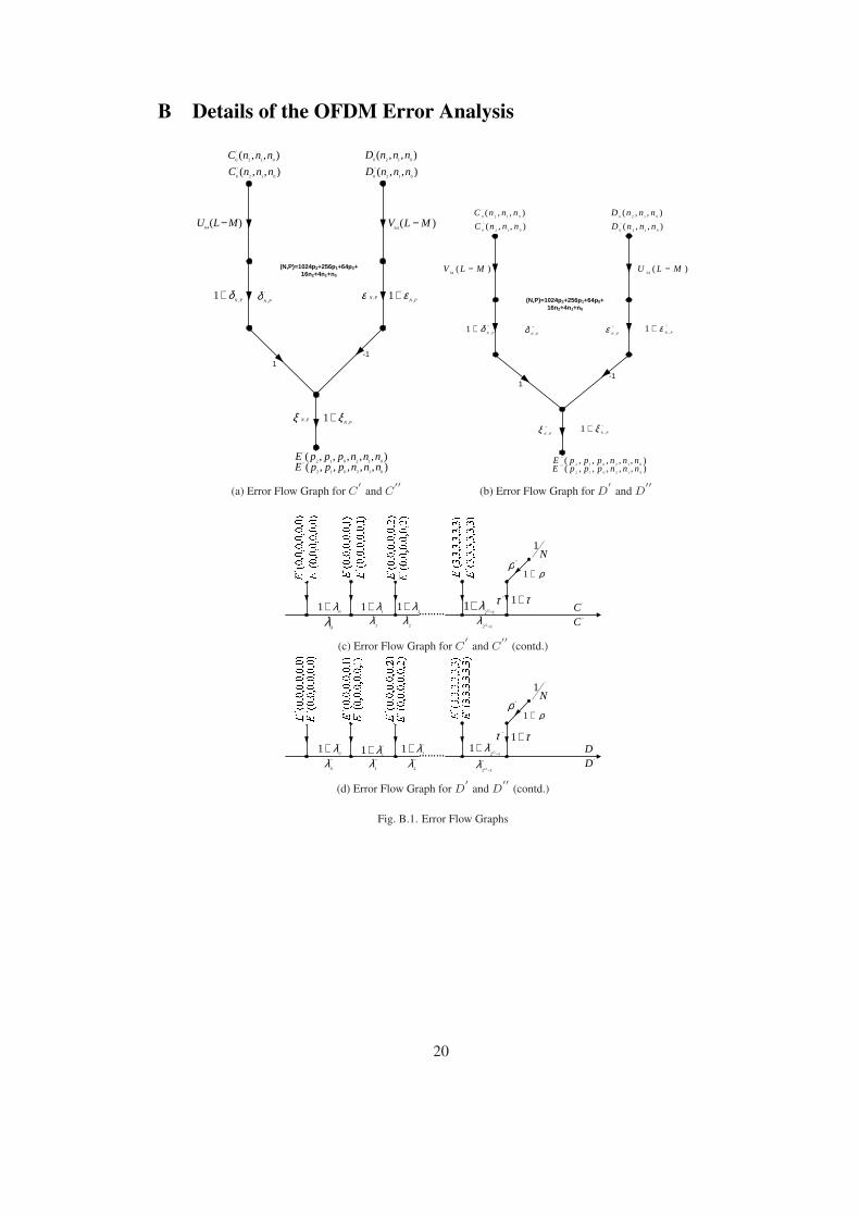
B Details of the OFDM Error Analysis

),,(012

''

0nnnC

),,(012

'

0nnnC

),,(012

''

0nnnD

),,(012

'

0nnnD

)(64

MLV −)(64

MLU −

'

,PNδPN ,

1 δ+PN ,

1 ε+

PN ,1 ξ+PN ,

'ξ

PN ,'ε

-11

),,,,,(012012

'' nnnpppE),,,,,(

012012

' nnnpppE

(N,P)=1024p2+256p1+64p0+16n2+4n1+n0

(a) Error Flow Graph for C′

and C′′

),,(012

''

0nnnC

),,(012

'

0nnnC

),,(012

''

0nnnD

),,(012

'

0nnnD

)(64

MLU −)(64

MLV −

'''

,PNδ''

,1

PNδ+ ''

,1

PNε+

''

,1

PNξ+'''

,PNξ

'''

,PNε

-11

),,,,,(012012

'''' nnnpppE),,,,,(

012012

''' nnnpppE

(N,P)=1024p2+256p1+64p0+16n2+4n1+n0

(b) Error Flow Graph for D′

and D′′

………

N1

''τ

ρ+1

τ+1

''ρ

01 λ+

11 λ+

21 λ+

12121

−+ λ

'

0λ '

1λ '

2λ

1212−λ

'C''C

(c) Error Flow Graph for C′

and C′′

(contd.)

………

N1

''τ

ρ+1

τ+1

''ρ

'D''D

''

01 λ+ ''

11 λ+ ''

21 λ+ ''

12121

−+ λ

'''

0λ '''

1λ '''

2λ '''

1212−λ

(d) Error Flow Graph for D′

and D′′

(contd.)

Fig. B.1. Error Flow Graphs

20

Code B.1

∀ x q0 q1 q2. ∃ f. (IFFT_FFT_REAL_TO_FP_ERROR x q0 q1 q2 =complex_64 * complex_sum (0,4) (λp0. complex_sum (0,4) (λp1.complex_sum (0,4) (λp2. complex_sum (0,4) (λn0. complex_sum (0,4)(λn1. complex_sum (0,4) (λn2.

ERROR_0 x n2 n1 n0 * OMEGA n0 n1 n2 p0 p1 p2 q0 q1 q2 +f n0 n1 n2 p0 p1 p2 q0 q1 q2))))))) ∧

∃ t l d e z t′ l′′ d′′ e′′ z′′. f n0 n1 n2 p0 p1 p2 q0 q1 q2 =complex ( Val (float_Re ((λn0 n1 n2. float_complex_round (x n0 n1n2)) n0 n1 n2)) *

Val (FLOAT_OMEGA_RE n0 n1 n2 p0 p1 p2 q0 q1 q2) *((1 + d n0 n1 n2 p0 p1 p2 q0 q1 q2) *(1 + z n0 n1 n2 p0 p1 p2 q0 q1 q2) *mul (ER_K n0 n1 n2 p0 p1 p2,4097 − ER_K n0 n1 n2 p0 p1 p2)(λi. 1 + l i) * (1 + t) − 1) −

Val (float_Im ((λn0 n1 n2. float_complex_round (x n0 n1 n2)) n0 n1 n2)) *Val (FLOAT_OMEGA_IM n0 n1 n2 p0 p1 p2 q0 q1 q2) *

((1 + e n0 n1 n2 p0 p1 p2 q0 q1 q2) *(1 + z n0 n1 n2 p0 p1 p2 q0 q1 q2) *mul (ER_K n0 n1 n2 p0 p1 p2,4097 − ER_K n0 n1 n2 p0 p1 p2)(λi. 1 + l i) * (1 + t) − 1),

Val (float_Re ((λn0 n1 n2. float_complex_round (x n0 n1 n2)) n0 n1 n2)) *Val (FLOAT_OMEGA_IM n0 n1 n2 p0 p1 p2 q0 q1 q2) *

((1 + d′′ n0 n1 n2 p0 p1 p2 q0 q1 q2) *(1 + z′′ n0 n1 n2 p0 p1 p2 q0 q1 q2) *mul (ER_K n0 n1 n2 p0 p1 p2,4097 − ER_K n0 n1 n2 p0 p1 p2)(λi. 1 + l′′ i) * (1 + t′) − 1) −

Val (float_Im ((λq0 q1 q2. float_complex_round (x q0 q1 q2)) q0 q1 q2)) *Val (FLOAT_OMEGA_IM n0 n1 n2 p0 p1 p2 q0 q1 q2) *

((1 + e n0 n1 n2 p0 p1 p2 q0 q1 q2) *(1 + z n0 n1 n2 p0 p1 p2 q0 q1 q2) *mul (ER_K n0 n1 n2 p0 p1 p2,4097 − ER_K n0 n1 n2 p0 p1 p2)

(λi. 1 + l i) * (1 + t′) − 1))

Code B.2

∀ X M V x q0 q1 q2. ∃ f′. (IFFT_FFT_REAL_TO_FXP_ERROR X M V x q0 q1 q2 =complex_64 *complex_sum (0,4) (λp0. complex_sum (0,4) (λp1.complex_sum (0,4) (λp2. complex_sum (0,4) (λn0.complex_sum (0,4) (λn1. complex_sum (0,4) (λn2.ERROR′_0 X M V x n2 n1 n0 * OMEGA n0 n1 n2 p0 p1 p2 q0 q1 q2 +f′ n0 n1 n2 p0 p1 p2 q0 q1 q2))))))) ∧∃t′ l′ d′ e′ z′ t′′′ l′ d′′′ e′′′ z′′′.f′ n0 n1 n2 p0 p1 p2 q0 q1 q2 =

complex (d′ n0 n1 n2 p0 p1 p2 q0 q1 q2 +e′ n0 n1 n2 p0 p1 p2 q0 q1 q2 +z′ n0 n1 n2 p0 p1 p2 q0 q1 q2 +sum (ER_K n0 n1 n2 p0 p1 p2,4096 −ER_K n0 n1 n2 p0 p1 p2)(λi. l′ i) + t′,d′′′ n0 n1 n2 p0 p1 p2 q0 q1 q2 +e′′′ n0 n1 n2 p0 p1 p2 q0 q1 q2 +z′′′ n0 n1 n2 p0 p1 p2 q0 q1 q2 +e′ n0 n1 n2 p0 p1 p2 q0 q1 q2 +sum (ER_K n0 n1 n2 p0 p1 p2,4096 −ER_K n0 n1 n2 p0 p1 p2) (λi. l′′′ i) + t′′′)

Code B.3

∀ X M V x q0 q1 q2. IFFT_FFT_FP_TO_FXP_ERROR X M V x q0 q1 q2= right−hand side of [ REAL to FP error theorem ] −right−hand side of [ REAL to FXP error theorem ]

21

Replace this file with prentcsmacro.sty for your meeting,or with entcsmacro.sty for your meeting. Both can befound at the ENTCS Macro Home Page.

The Impact of Drifting Clocks on ZigBee’s

Energy Efficiency

and why formal methods are pivotal to assess that

Holger Hermanns

Dependable Systems and SoftwareSaarland University

Saarbrucken, Germany

and

Validation de SystemesINRIA Rhone AlpesGrenoble, France

Wireless embedded sensor networks are predicted to provide attractive appli-

cation possibilities in industry as well as at home. IEEE 802.15.4 and ZigBee are

proposed as standards for such networks with a particular focus on pairing reliability

with energy efficiency, while sacrificing high data rates. IEEE 802.15.4 is config-

urable in many aspects, including the synchronicity of the communication, and the

periodicity in which battery-powered sensors need to wake up to communicate.

In recent work, we have developed formal behavioural models of the energy

implications of these options [1]. The models are modularly specified using the

language MoDeST [2], which has a rigorous compositional semantics mapping on

stochastic timed automata. The latter are simulated using a variant of discrete-event

simulation implemented in the tool Mobius [3]. We managed to estimate energy

consumptions of a number of possible communication scenarios in accordance with

the standards, and derived very interesting conclusions about the energy optimal

configuration of such networks. As a specific fine point, we investigated the effects

of drifting clocks on the energy behavior of various application scenarios.

In this talk, I will review this joint work with Christian Groß and Reza Pulungan.

I will give a detailled account of the formal modelling and analysis approach taken,

and will point out why the use of formal methods appears as the only reliable as

well as practical way to study such intricate questions.

References

[1] C. Groß, H. Hermanns, R. Pulungan. Does Clock Precision Influence ZigBee’s Energy Consumptions?.In OPODIS 2007, LNCS 4878:174-188, 2007.

c©2008 Published by Elsevier Science B. V.

Hermanns

[2] H. C. Bohnenkamp, P. R. D’Argenio, H. Hermanns, and J.-P. Katoen. MoDeST: A compositionalmodeling formalism for hard and softly timed systems. IEEE Trans.Soft.Eng., 32(10):812–830, 2006.

[3] D. Daly, D. D. Deavours, J. M. Doyle, P. G. Webster, and W. H. Sanders. Mobius: An extensible toolfor performance and dependability modeling. In TOOLS 2000, LNCS 1786:332–336, 2000.

2

Performance Evaluation of Sensor Medium Access Control Protocol Using Coloured Petri Nets

Mohammad Abdollahi Azgomi and Ali Khalili

Department of Computer Engineering, Iran University of Science and Technology, Tehran, Iran

azgomi@iust.ac.ir and al_khalili@comp.iust.ac.ir

Abstract. Formal modelling techniques can be used for analysis of wireless sensor networks (WSNs). Coloured Petri nets (CPNs) that is an extension of Petri nets is a powerful modelling technique. In this paper, we present a CPN model for modelling and performance evaluation of a medium access control protocol in WSNs named sensor-medium access control protocol (S-MAC). S-MAC is an energy-aware MAC protocol with nodes scheduling. The pro-posed model for this protocol uses the hierarchical modelling capability of CPNs. By using CPNs in this case study and the proposed method for model-ling packet broadcast, we have demonstrated the possibility of modelling and evaluation of any other MAC protocol in WSNs or mobile ad-hoc networks (MANET).

1 Introduction

Wireless sensor networks (WSNs) consist of a set of small, cheap, and low-power sensor nodes that use wireless technology for communications. Comparing to other types of networks, WSNs have some notable limitations, such as processing ability, memory capacity and battery life-time. As a result of these limitations and the re-quirements for some new protocols, much research is engaged in this field [1].

The general approach for analysis of WSNs is to use the existing simulation tools or simulators, such as OPNET [2], NS-2 [3] and etc. For using these tools, we must consider that the result of simulating an algorithm may be different, depending on the selected tool, because of important divergence between simulators [4]. An alternative to simulation is to employ formal modelling and analysis techniques. Using these techniques, both performance evaluation and model checking can be performed. While this approach is widely used in traditional networks, advanced WSNs algo-rithms and protocols present a set of challenges to be formally modelled by the exist-ing methods and tools, some of which are addressed in [5].

Coloured Petri nets (CPNs) [6], which are an extension of Petri nets, are an appro-priate modelling language. CPNs have a graphical notation that is based on an under-lying mathematical definition and provide several analysis methods, including simu-lation, state space analysis and invariant analysis. A major benefit of using CPNs is to obtain complete and unambiguous specifications of system behaviour.

As a case study, we have used CPNs and CPN Tools [14] for performance evalua-tion of sensor-medium access control protocol (S-MAC). The results are presented in this paper.

The remainder of the paper is organized as follows. In section 2, we report the re-lated works. In section 3, an informal description of S-MAC protocol is provided. Section 4, describes the modelling approach used in the case study and the conse-quent results are given in section 5. Finally, some concluding remarks are mentioned in section 6.

2 Related Works

A lot of results are reported in literature, which have used formal techniques for mod-elling and analysis of traditional networks. In [7], Petri nets are used for modelling IEEE802.3 protocol in a traditional local area network (LAN) to construct a detailed model. The model is used to evaluate some performance measures. In [8], a high-level Petri net named finite population queuing system Petri nets (FPQSPN) is intro-duced for modelling and simulation of medium access control layer in computer net-works.

Given the increasing sophistication of WSN algorithms and the difficulty of modi-fying an algorithm once the network is deployed, there is a clear need to use formal methods to validate system performance or functionality prior to implementing such algorithms [5]. In published works, different approaches have been used for specify-ing and modelling sensor networks. In these works, based on the requirements for performance evaluation or model checking purposes, a modelling technique has been selected and employed. Some new extensions of Petri nets are also proposed for these purposes, which use some extra information in places [9] or dynamic configuration capability [10] in Petri nets structure. Such extensions, attempt to extend Petri nets to model dynamic behaviour of WSNs, such as mobility of nodes, node death (as a re-sult of battery limitation) or node failures. In [11], Petri nets are used for modelling and simulation of a routing protocol in a mobile ad-hoc network (MANET). In this work, a topology approximation mechanism is proposed to address mobility problem and performs simulation to show that this mechanism can indeed mimic the mobility of a MANET.

3 Sensor Medium Access Control Protocol

Since we will use the specification and operations of S-MAC in the next sections, we will briefly review this protocol in the following paragraphs, which is based on [13].

The open system interconnection (OSI) model defines a layered architecture for network protocols. The medium access control (MAC) layer is responsible for deter-mining which node is allowed to access underlying layer (i.e. physical medium) at any moment. One fundamental task of a MAC protocol is to avoid simultaneous transmissions (i.e. collision) and the basic mechanism used for reducing the possibil-

ity of collision in contention based MAC is referred to as carrier sense, multiple ac-cess (CSMA). In this mechanism each node, before starting a transmission, senses the medium to find it clear and then starts its transmission.

In wireless environment, IEEE802.11 protocol [12] is a family of standards which introduces a number of MAC schemes and the physical (PHY) layer for WLAN. The primary MAC scheme of the standard is called distributed coordination function (DCF) and has two variants: basic access (BA) and request to send/clear to send (RTS/CTS). The BA scheme (that is also known as two-way handshaking scheme), has the simplicity advantage, but the possibility of (large) data packet is somewhat high and thus can cause to waste energy and degrade performance. In RTS/CTS scheme, the same sensing/randomised backoff procedure of the BA scheme is used but an additional handshake is involved using RTS and CTS control packets (as a result, this scheme is referred to as four-way handshake). After sensing that the me-dium is free, a station wishing to send data packets over the medium sends an RTS packet, which includes information on the duration of subsequent transmissions. On reception of an RTS, the destination replies with a CTS packet. The sender will start the transmission of actual data packets on reception of the CTS confirmation. Every neighbouring node overhearing the RTS/CTS exchange is aware of the future com-munication duration hence refrains from attempting to access the medium for the whole duration of the communication.

The IEEE802.11 is used in some wireless sensor networks. Considering the attrib-utes and limitations of WSNs, we need some special protocols that designed for them. In WSNs, one of the important requirements is efficient usage of energy to prolong network lifetime and must be considered in any aspect of communication protocols, routing algorithms and query processing approach. The so-called S-MAC scheme [13] is designed to reduce energy consumption of communicating nodes. It is based on a simple observation that for most WSN applications, the sensed data streams are generated at low frequency (there is nothing to be sensed at most of the time.).

Designing S-MAC aims at reducing energy consumption from all sources of en-ergy waste (i.e. idle listening, collision, overhearing and control overhead). The pro-tocol is based on two distinct operational states for sensing nodes, an energy expen-sive LISTEN mode where the radio of a node is switched on, and an energy saving SLEEP mode in which the radio is turned off. Each node uses a periodic listen/sleep schedule to switch between LISTEN/SLEEP operational modes. A complete LISTEN/SLEEP cycle is referred to as a frame and the duty cycle is the ratio of the listen interval to frame length which can be adapted according to the application re-quirements. The S-MAC scheme is concerned with two different aspects: choosing and maintaining of sleeping schedules for each node (usually referred to as coordi-nated sleeping) and collision avoidance. Coordinated Sleeping. Each node maintains a schedule table where the LISTEN/SLEEP period of each of its neighbours is recorded. When a node wants to send some data to one of its neighbours, it will start the RTS/CTS protocol during the LISTEN phase of the destination node, whose details are retrieved from the schedule table. The schedule table is built in a distributed fashion, through broadcasting of SYNC packets between neighbouring nodes. A SYNC packet contains the sender’s chosen schedule. Each node either chooses its own schedule or follows a schedule

received from one of its neighbours. As soon as a node picks a schedule, it broadcasts it so that all neighbours can update their table. Although the aim of coordinated sleep-ing is to synchronise neighbouring nodes on a single and shared schedule, it is possi-ble for neighbouring nodes to have different schedules. This happens whenever a node that has announced its own schedule receives a different schedule from one of its neighbours. Anyhow, a node may receive different schedules from its neighbours and in this case, it must behave based on its schedule table for sending a packet to any node. Collision Avoidance. This is achieved through the 802.11 MAC. The RTS/CTS protocol is used to avoid collision for unicast packets, whereas a randomised carrier sense is used to prevent simultaneous transmission of broadcast packets (i.e. SYNC). A unicast data packet follows the sequence RTC/CTS/DATA/ACK. After a success-ful RTS/CTS exchange, the corresponding sender and receiver will temporarily ig-nore their sleeping schedule until the data transmission is complete. They will then revert to SLEEP mode, until their next LISTEN mode is scheduled. This technique with the aid of network allocation vector (NAV) variable can solve the hidden termi-nal problem.

4 Modelling S-MAC with CPNs

In this section, we describe our proposed coloured Petri net (CPN) model for S-MAC. The global model has been constructed taking the advantage of the hierarchical capa-bilities of CPNs [6]. Hierarchical CPN allows the construction of a large model as a set of smaller models connected to each other using well-defined interfaces (i.e. sub-stitution transitions). In this way, a complex model, like the one we will present in this section, can be reduced to constructing some smaller models. The model aims to be as detailed as possible (i.e. it tries to model all operations of the MAC layer and scheduling of nodes).

Like [13], topology of the model is a two-hop network with two sources and two sinks, as shown in Fig. 1. Packets from the sources, A and B, flow through the node C and will end at sinks, D and E. Each node has a buffer containing received packets. For simplicity, we assumed that the size of the buffer is one packet. In addition, the collision may occur in network. Consider that this collision can occur only in control packets (i.e. SYNC or RTS/CTS) and data packets do not collide. We assume that the transmission media is ideal and noise-free and thus, every sent packet will receive to its destination node. It may also encounter a collision. We have also assumed that there is not any queueing and backoff delay as in [13]. We assumed that the propaga-tion and processing delays can be ignored, too. In this case, only carrier sense delay, transmission delay and sleep delay are taken into account. Consider that transmission delay depends on packet size and is a constant value for each type of packet and thus large packets (e.g. data packets) have a larger transmission delay than small packets (e.g. control packets).

To describe the model, we will first explain the main part of the model and higher level of the model hierarchy. Then submodels will be described. For constructing and

analysing the model, we have used the CPN Tools [14], which is a well-known and powerful tool for modelling and analysis of CPNs.

Fig. 1. Topology of the model, two-hop network with two sources and two sinks.

4.1 CPN Model for Wireless Channel

In wireless media model, if a node sends a packet, the media must broadcast it to all nodes. Each node can “hear” the packet if and only if the source of the packet is one of the neighbours. In this model, when a node transmits a packet, the packet is deliv-ered by all nodes according to their sequence numbers. When a node gets a packet, checks the source of the packet and if it is a neighbour node, it will “hear” the packet. Anyhow, the packet is given to the channel for delivering to the next node. If the packet is delivered by all nodes, the channel drops the packet. Because there is no propagation delay, this operation must be performed without any time consumption and all nodes will deliver the packet at the same time. Here, we assume that nodes have not any movement, but considering this approach for modelling broadcast be-haviour, we can have mobile nodes (e.g. in mobile wireless sensor or ad-hoc net-work). In mobile networks, neighbouring detection is performed dynamically based on physical location of nodes and radio transmission range.

Fig. 2 shows model of the wireless channel and network nodes as substitution tran-sitions for a network with two nodes. The hierarchical capability of CPNs provides scalability of the model in the network.

Fig. 2. Main part of wireless channel model with only two nodes (nodes are modelled as substi-

tution transitions).

4.2 CPN Model of Nodes

In this subsection we describe CPN submodels for node scheduling, table of neighbours scheduling, sending a message and listening to channel.

Node Scheduling. In S-MAC protocol, each node has a constant sleep and wakeup period. First (and after a small random period of time), each node chooses his own scheduling and announces it to its neighbours using a SYNC message. The SYNC message shows the beginning of the wakeup time. In sleep mode, nodes turn off the radio to save energy. In wakeup period, a node for transmitting a packet must sense the channel and if the channel is free (physically and virtually), it sends RTS packet and waits for CTS confirmation. Then, it sends the data packet and waits for the acknowledgment. The basic part of the model is shown in Fig. 3. The right side of the figure illustrates neighbours schedule table and the left side, models the synchronisation procedure.

Fig. 3. Basic part of node scheduling model.

Table of Neighbours Scheduling. In each node, there exists a table that contains scheduling information of its neighbours. Model of this table is illustrated in right side of Fig. 3. When a SYNC packet is received by a node, the required information can be obtained from the packet for updating schedule table. By assuming predefined and constant values for sleep and wakeup periods, each node can update and maintain this table independently and achieve target node scheduling at any time.

Sending a Message. Transmitting a message to a neighbour node is performed based on neighbours schedule table. In this case, after determining channel state, if the channel is free, the packet will be sent based on the information retrieved from schedule table. Fig. 4 shows the basic part of message transmission model.

4.3 Hierarchical Model

The hierarchical structure of the composed CPN model is illustrated in Fig. 6. The wireless channel model is in the highest level of the model hierarchy that models the physical layer and broadcast communications. In the next level, models of network nodes exists that model basic behaviour of the nodes and in the lowest level, there are some submodels that model the nodes behaviour in detail.

In general, using hierarchical structure of CPNs facilitates modelling complicated and large systems. In addition, this capability provides scalability to easily change the topology of the network and the number of nodes.

Fig. 4. The basic part of message transmission model that shows the message transmission procedure stages (channel state retrieval, sending RTS, receiving CTS and sending ACK).

Fig. 5.The basic part of listening to the channel model.

Fig. 6. Hierarchical architecture of the CPN model (for a network with four nodes).

5 Simulation Results

After constructing the model, we can extract the related performance measures using model simulation. In CPN Tools, this goal can be achieved using the monitor mecha-nism. A monitor is a mechanism in CPN Tools that is used to observe, inspect, con-trol, or modify the simulation of a CPN model and the desired measures. In our study of S-MAC protocol, performance measures include energy consumption and packet delivery delay. For example, result of the model simulation for average energy con-sumption in source nodes for transmission of some constant data packets versus mes-sage inter-arrival time with duty cycle 20% and 50% is shown in Fig. 7. More meas-ures may be defined and computed in a similar way.

6 Conclusions

In this paper, we presented a CPN model for S-MAC protocol. S-MAC is a medium access control protocol introduced for wireless sensor networks with the aim of re-ducing energy consumption. Using the hierarchical capability of CPNs, we have modelled a wireless environment (wireless media and network nodes). Then, we have evaluated some performance measures by using CPN Tools and its simulation fea-tures.

Fig. 7. Simulation results for average energy consumption in source nodes versus message

inter-arrival time.

Results of this case study can help the design process of a real network. Modelling enough details in this model, shows the capabilities of CPNs for modelling and evaluation of wireless sensor and ad-hoc networks. Using hierarchical CPNs to model WSNs and its protocols have two main advantages that are flexibility and scalability of model construction.

As a future work, we intend to construct a comprehensive model for mobile sensor networks. We are attempting to add a routing protocol to this model by employing the hierarchical capability of CPNs.

References

1. Akyildiz, I.A., Su, W., Sankarasubramaniam, Y., Cayirci, E.: A Survey of Sensor Networks, IEEE Communication Magazine, Vol. 40 (2002) 102–115.

2. OPNET Modeler, URL: http://www.opnet.com/products/modeler/home.html. 3. ns-2 network simulator, URL: http://www.isi.edu/nsnam/ns/. 4. Cavin, D., Sasson, Y., Schiper, A.: On the Accuracy of MANET Simulators, Proc. of

POMC, ACM Press (2002) 38–43. 5. Ölveczky, P.C., Thorvaldsen, S.: Formal Modeling and Analysis of the OGDC Wireless

Sensor Network Algorithm in Real-Time Maude, Lecture Notes in Computer Science , Vol. 448 , Springer Berlin Heidelberg (2007) 1611-3349.

6. Jensen, K.: Coloured Petri Nets. Basic Concepts, Analysis Methods and Practical Use, Vol-umes 1-3, Basic Concepts. Monographs in Theoretical Computer Science, Springer-Verlag (1997).

7. Morera, P.H., Gonzalez, T.M.P.: A CPN Model of the MAC Layer. In K.Jensen (ed.): Pro-ceedings of the 2nd Workshop on Practical Use of Coloured Petri Nets and Design/CPN, Aarhus (1999) 153-172

8. Čapek, J.: Petri Net Simulation of Non-deterministic MAC Layers of Computer Communi-cation Networks, Ph.D. Thesis, Czech Technical University (2003).

9. Luo, Y., Tsai, J.J.P.: A Graphical Simulation System for Modeling and Analysis of Sensor Networks, Proc. of the 7th IEEE Int’l Symp. on Multimedia (2005).

10. Graff, C.J., Giardina, C.: Dynamic Petri Nets: A New Modelling Technique for Sensor and Distributed Concurrent Systems, Proc. of the IEEE Military Communications Conf. (2005).

11. Xiong, C., Murata, T., Tsai, J.: Modeling and Simulation of Routing Protocol for Mobile Ad hoc Networks Using Coloured Petri Nets, Proc. of Workshop on Formal Methods Ap-plied to Defense Systems (2002) 145-153.

12. Wireless LAN Medium Access Control (MAC) and Physical Layer (PHY) Specification, IEEE Std. 802.11 (1999).

13. Ye, W., Heidemann, J., Estrin, D.: An Energy-Efficient MAC Protocol for Wireless Sensor Networks, IEEE/ACM transaction on networking, Vol. 12, No. 3 (2004).

14. CPN Tools, URL: http://wiki.daimi.au.dk/cpntools/.

Replace this file with prentcsmacro.sty for your meeting,or with entcsmacro.sty for your meeting. Both can befound at the ENTCS Macro Home Page.

Validating Wireless Congestion Control andReliability Protocols using ProB and Rodin

Jens Bendisposto, Michael Jastram, Michael LeuschelChristian Lochert, Bjorn Scheuermann, Ingo Weigelt1,2

Computer Science DepartmentHeinrich Heine University

Dusseldorf, Germany

Abstract

Implicit hop-by-hop congestion control is a novel congestion control paradigm for wireless multihop net-works. Implemented in the CXCC protocol, it has already proven its performance in simulations andmeasurements. Since CXCC makes extensive use of the properties of an inherently unreliable medium, itis, however, vitally necessary to validate the correctness of the protocol. Indeed, an early version of theCXCC protocol contained deadlocks. CXCC is complemented by an end-to-end reliability mechanism inthe BarRel transport protocol. In combination, both protocols offer TCP-equivalent service in dynamicwireless multihop environments, including, e.g., route changes. BarRel relies on properties of CXCC. Ittherefore likewise deserves validation.In this work we attempt to validate the CXCC and BarRel protocols using formal methods. To this end,we are developing various models in B and Event-B. We are using the ProB tool to animate and modelcheck the formal models and the Rodin platform to formally prove correctness properties. In this paper wepresent first encouraging steps towards a full formal validation of the protocols.

Keywords: Protocol Validation, Wireless Networks, Congestion Control, End-to-End Reliability, CXCC,BarRel, B-Method, ProB, Rodin

1 Implicit Hop-by-Hop Congestion Control

In previous work we have introduced the Cooperative Cross-layer Congestion Con-trol (CXCC) protocol and the Backpressure Reliability (BarRel) protocol. CXCC isa congestion control approach, and BarRel is the corresponding end-to-end reliabil-ity mechanism. Both protocols in combination provide TCP-equivalent end-to-endservice. In this section, we briefly outline CXCC and BarRel. For a more detaileddiscussion, we refer the reader to [6, 7].

1.1 CXCC

CXCC is a cross-layer approach, encompassing essentially the MAC and transportlayers. It uses implicitly obtained information for hop-by-hop backpressure conges-

1 Email: {bendisposto,jasteam,leuschel,lochert,scheuermann}@cs.uni-duesseldorf.de2 The authors are grateful to the German Research Foundation (DFG) and the EU funded FP7 researchproject 214158 DEPLOY for partially funding this research.

c©2008 Published by Elsevier Science B. V.

Bendisposto et al.

tion control and single-hop reliability. The key concept is that, for each end-to-endconnection, an intermediate node may only forward a packet towards the destina-tion after its successor along the route has forwarded the previous one. This yieldsa backpressure mechanism which reacts very rapidly to varying medium conditionsand effectively avoids excessive packet inflow into congested network areas.

The CXCC protocol realizes the implicit hop-by-hop congestion control principleby overhearing the medium after a transmission. No further packets for the sameconnection may be transmitted, until the packet has been forwarded further by thedownstream node. The connection is “blocked” at the first node until the secondnode forwards the packet further on (see Fig. A.1 in appendix). In such a setting,overhearing the transmission of the downstream node can serve a dual purpose: itconstitutes an implicit acknowledgment, indicating the successful reception of theprevious packet by the downstream node, and at the same time is a signal to unblockthe connection, allowing the next packet to be transmitted.

Link layer acknowledgments as in IEEE 802.11 are, consequently, not necessary.Just at the last hop the packet is therefore acknowledged explicitly. However, wire-less communication is very error-prone. Transmissions may be lost, for instance,due to a collision. CXCC uses Request For Acknowledgment (RFA) packets in or-der to overcome such situations. An RFA is a small control packet, containing justenough information to identify the packet it refers to. Upon reception of an RFA,a node checks whether it already has received the respective data packet or not. Itmay then provide appropriate feedback, such that, if necessary, the transmission isrepeated. For details see [7].

1.2 BarRel

The CXCC retransmission mechanisms allow to overcome individual transmissionerrors between adjacent nodes along the route. Because CXCC limits the numberof packets per hop to one, there will, by construction, also be no packet loss due tobuffer overflows. Hence, there will be no packet loss with CXCC as long as the routeto the destination remains stable. In this situation, a source node can implicitlyobtain information about successful packet deliveries to the destination node: thereis at most one packet per hop in CXCC, and there is neither packet loss nor packetreodering in the network. Consequently, if the route to the destination is currentlyn hops long, after the (i + n)-th packet of a transmission has left the source node,the i-th packet must have arrived at the destination.

In BarRel, this is used in order to realize TCP-equivalent reliable end-to-enddata transport without the need for a continuous stream of end-to-end acknowl-edgment traffic. In wireless multihop environments, such acknowledgment traffic isconsidered a major problem, because it is forwarded over the same wireless mediumas the data traffic (in opposite direction), causing significant overhead and frequentcollisions. Therefore, an ACK-free reliable transport protocol is highly desirable.

However, it may also happen that a wireless link fails permanently. Then, theabove assumptions do not necessarily hold true, and packet loss may happen. Ifone node along the route is no longer reachable, the routing protocol used in thenetwork will discover a new route. In order to guarantee end-to-end reliability also

2

Bendisposto et al.

in case of link breaks and re-routing, the BarRel mechanism steps into the breach.When re-routing occurs, a BarRel source node will go back to the first packet forwhich it could not yet confirm successful delivery, and retransmit from there.

The delivery of the last n packets of a packet burst can not be acknowledgedas described above. BarRel therefore includes further mechanisms to confirm theirarrival at the destination. For this, it possible to add a number of empty packets atthe end of the transmission. By the abovementioned implicit delivery confirmationmechanism, when the n-th such “capacity refill” (CaRe) packet leaves the sourcenode, it is known that the last data packet must have successfully arrived. Thisallows for a protocol operation without any oncoming end-to-end control traffic.For details see [6].

2 Validating CXCC and BarRel

The B-method [1] is a formal methodology for the systematic development of safety-critical software systems, based on the idea of refinement. Event-B (e.g., [4]) is thesuccessor of the B-method, which is also suitable to model reactive systems. Bothare supported by industrial-strength proving tools. Event-B now spurts the Rodinplatform [2] which enables integrated editing and proof. Our ProB tool [5] can beused to animate B and Event-B models, as well as validate temporal logic formulasvia model checking.

In this paper, we decided to use the Event-B method to verify the correctnessof BarRel and CXCC; in future work we also plan to investigate the use of theCSP process algebra (which is also supported by our tool ProB). Our goal is tovalidate the CXCC and BarRel protocols using animation and model checking, butalso to try and develop a version of the algorithm which is correct by design. Wealso want to evaluate if the B Method and the tools ProB [5] and Rodin [2] areappropriate for the design of networks protocols. For the verification we developedtwo different sets of formal models. The first version was a set of models used foranimation and model checking rather than for proof. The goal was to get familiarwith the problems that arise from the domain. Also we wanted to gain confidencein the correctness of the protocols. The second model is used to obtain correctnessby design, by refining a very abstract model towards the CXCC/BarRel protocols.

2.1 First version: models for animation

We specified CXCC and BarRel in two different models. The CXCC model containsa cycle free sequence of nodes, the route, for an end-to-end connection. The nodesare equipped with two buffers, one for incoming packets and one to buffer packetssent. The model can put packets into on end of the route and remove them fromthe other end. During transmission we can lose packets and acknowledgements andit is also possible that the implicit acknowledgment gets lost. The model does notyet cope with multiple packets on multiple routes. We also developed a graphicalrepresentation that could be used to demonstrate the protocol to domain expertswho are not familiar with the mathematical notation. The absences of deadlockswas validated using ProB, as were several LTL formulas specifying correct deliveryunder certain fairness assumptions.

3

Bendisposto et al.

2.2 Second version: models for proof

A flow in a CXCC enabled network can be abstractly seen as a queue. The senderadds data packets to it and the receiver removes them. Another constraint resultingfrom CXCC and BarRel is that we can divide this queue into different contiguoussections. Each section contains only data-packets, CaRe-packets or duplicates ofreceived data-packets. Furthermore CaRe-packets can only form the last section ofthe queue and duplicates precede data.

The first model m0 defines a generic Queue, mainly modeled after [3]. Methodsto enqueue, dequeue and delete the whole Queue have been implemented. Thisqueue will then subsequently be refined until the detailed behaviour of CXCC andBarRel is obtained.

m0 is then refined to map the queue elements to links along the route holdingdata packets. Accordingly the maximum size of the Queue is limited to the route-length. The events enqueue and dequeue now represent sending and receiving databy the source and receiver. A routebreak refines the delete event to additionallyreset the counter used by the sender. As another step towards realistic networkconditions the routelength is now nondeterministically changed by this event.

The next refinement step is to introduce CaRe packets. At this refinement stepthe queue section for CaRe packets is simply represented by a number holding thenumber of packets in it. Accordingly two new events sendCaRe and receiveCaReare modeled that simply incremend and decrement respectively this value.

The routebreak event in m1 removes all elements in the queue and resetsthe senders counter to retransmit exactly the lost packets. In m3, we removeroutelength many packets. This reflects, that the sender must assume the worst

case. As a result, the receiver now has to cope with duplicate packets arriving.An animation of the last model with ProB can be seen in Fig. B.1 in the ap-

pendix for referees. As far as proving is concerned, m0 and m3 still contain oneunproven proof obligation (POs) each (out of 57 and 7 resp.). Models m1 and m2are fully proven, where 88 of 94 and 69 of 78 POs were automatically proven.

References

[1] Abrial, J.-R., “The B-Book,” Cambridge University Press, 1996.

[2] Abrial, J.-R., M. Butler and S. Hallerstede, An open extensible tool environment for Event-B., in:ICFEM06, LNCS 4260 (2006), pp. 588–605.

[3] Abrial, J.-R. and D. Cansell, Formal construction of a non-blocking concurrent queue algorithm (a casestudy in atomicity), Journal of Universal Computer Science 11 (2005), pp. 744–770.

[4] Abrial, J.-R., D. Cansell and D. Mery, Refinement and reachability in Eventb, in: H. Treharne, S. King,M. C. Henson and S. A. Schneider, editors, ZB, Lecture Notes in Computer Science 3455 (2005), pp.222–241.

[5] Leuschel, M. and M. Butler, ProB: A model checker for B, in: K. Araki, S. Gnesi and D. Mandrioli,editors, FME 2003: Formal Methods, LNCS 2805 (2003), pp. 855–874.

[6] Scheuermann, B., “Reading Between the Packets – Implicit Feedback in Wireless Multihop Networks,”Ph.D. thesis, Heinrich Heine University, Dusseldorf, Germany (2007).

[7] Scheuermann, B., C. Lochert and M. Mauve, Implicit hop-by-hop congestion control in wireless multihopnetworks, Elsevier Ad Hoc Networks 6 (2008), pp. 260–286.

4

Bendisposto et al.

A Figures (for referees)

Fig. A.1. Packet forwarding in the CXCC protocol.

B Screenshots (for referees)

Fig. B.1. Third refinement animated with ProB for Rodin

5