preliminarysolutions ucdavis analysis
DESCRIPTION
AnalysisTRANSCRIPT

Analysis Preliminary Exams Solutions Guide
UC Davis Department of Mathematics
The Galois GroupFirst Edition: Summer 2010
August 31, 2011
Project Leader:Jeffrey Anderson
Solutions Correspondants:Luke Grecki
Nathan HannonRicky KwokOwen Lewis
Bailey MeekerMohammad OmarDavid RenfrewGreg ShinaultAdam Sorkin
Mathew Stamps

Contents
1 Building Up to the Exam 31.1 Your Graduate Education in Mathematics . . . . . . . . . . . . . 31.2 Exam Specifications . . . . . . . . . . . . . . . . . . . . . . . . . 41.3 Using These Solutions . . . . . . . . . . . . . . . . . . . . . . . . 5
2 References and Study Aids 62.1 Reference Texts in Analysis . . . . . . . . . . . . . . . . . . . . . 6
2.1.1 Berkeley Problems in Mathematics by Souza and Silva . . 72.1.2 Foundations of Mathematical Analysis by Johnsonbaugh
and Pfaffenberger . . . . . . . . . . . . . . . . . . . . . . . 82.1.3 Principles of Mathematical Analysis by Rudin . . . . . . . 92.1.4 Fourier Analysis by Kammler . . . . . . . . . . . . . . . . 102.1.5 Real and Complex Analysis by Rudin . . . . . . . . . . . 112.1.6 Real Analysis by Folland . . . . . . . . . . . . . . . . . . 122.1.7 Analysis by Lieb and Loss . . . . . . . . . . . . . . . . . 132.1.8 Applied Analysis by Hunter and Nachtergaele . . . . . . . 142.1.9 Measure Theory by Cohn . . . . . . . . . . . . . . . . . . 152.1.10 Functional Analysis by Reed and Simon . . . . . . . . . . 16
3 Fall 2002 173.0.11 Problem 6 . . . . . . . . . . . . . . . . . . . . . . . . . . . 173.0.12 Problem 7 . . . . . . . . . . . . . . . . . . . . . . . . . . . 183.0.13 Problem 8 . . . . . . . . . . . . . . . . . . . . . . . . . . . 193.0.14 Problem 9 . . . . . . . . . . . . . . . . . . . . . . . . . . . 203.0.15 Problem 10 . . . . . . . . . . . . . . . . . . . . . . . . . . 213.0.16 Problem 11 . . . . . . . . . . . . . . . . . . . . . . . . . . 22
4 Winter 2002 234.0.17 Problem 1 . . . . . . . . . . . . . . . . . . . . . . . . . . . 234.0.18 Problem 2 . . . . . . . . . . . . . . . . . . . . . . . . . . . 254.0.19 Problem 3 . . . . . . . . . . . . . . . . . . . . . . . . . . . 264.0.20 Problem 4 . . . . . . . . . . . . . . . . . . . . . . . . . . . 274.0.21 Problem 5 . . . . . . . . . . . . . . . . . . . . . . . . . . . 284.0.22 Problem 6 . . . . . . . . . . . . . . . . . . . . . . . . . . . 29
2

5 Winter 2005 305.0.23 Problem 1 . . . . . . . . . . . . . . . . . . . . . . . . . . . 305.0.24 Problem 2 . . . . . . . . . . . . . . . . . . . . . . . . . . . 335.0.25 Problem 3 . . . . . . . . . . . . . . . . . . . . . . . . . . . 345.0.26 Problem 4 . . . . . . . . . . . . . . . . . . . . . . . . . . . 365.0.27 Problem 5 . . . . . . . . . . . . . . . . . . . . . . . . . . . 385.0.28 Problem 6 . . . . . . . . . . . . . . . . . . . . . . . . . . . 39
6 Fall 2007 406.0.29 Problem 1 . . . . . . . . . . . . . . . . . . . . . . . . . . . 406.0.30 Problem 2 . . . . . . . . . . . . . . . . . . . . . . . . . . . 416.0.31 Problem 1 . . . . . . . . . . . . . . . . . . . . . . . . . . . 416.0.32 Problem 3 . . . . . . . . . . . . . . . . . . . . . . . . . . . 426.0.33 Problem 4 . . . . . . . . . . . . . . . . . . . . . . . . . . . 436.0.34 Problem 5 . . . . . . . . . . . . . . . . . . . . . . . . . . . 44
7 Winter 2008 467.0.35 Problem 1 . . . . . . . . . . . . . . . . . . . . . . . . . . . 467.0.36 Problem 2 . . . . . . . . . . . . . . . . . . . . . . . . . . . 477.0.37 Problem 3 . . . . . . . . . . . . . . . . . . . . . . . . . . . 487.0.38 Problem 4 . . . . . . . . . . . . . . . . . . . . . . . . . . . 507.0.39 Problem 5 . . . . . . . . . . . . . . . . . . . . . . . . . . . 517.0.40 Problem 6 . . . . . . . . . . . . . . . . . . . . . . . . . . . 53
8 Fall 2008 548.0.41 Problem 1 . . . . . . . . . . . . . . . . . . . . . . . . . . . 548.0.42 Problem 2 . . . . . . . . . . . . . . . . . . . . . . . . . . . 568.0.43 Problem 3 . . . . . . . . . . . . . . . . . . . . . . . . . . . 578.0.44 Problem 4 . . . . . . . . . . . . . . . . . . . . . . . . . . . 588.0.45 Problem 5 . . . . . . . . . . . . . . . . . . . . . . . . . . . 598.0.46 Problem 6 . . . . . . . . . . . . . . . . . . . . . . . . . . . 61
9 Winter 2009 629.0.47 Problem 1 . . . . . . . . . . . . . . . . . . . . . . . . . . . 629.0.48 Problem 2 . . . . . . . . . . . . . . . . . . . . . . . . . . . 649.0.49 Problem 3 . . . . . . . . . . . . . . . . . . . . . . . . . . . 659.0.50 Problem 4 . . . . . . . . . . . . . . . . . . . . . . . . . . . 679.0.51 Problem 5 . . . . . . . . . . . . . . . . . . . . . . . . . . . 699.0.52 Problem 6 . . . . . . . . . . . . . . . . . . . . . . . . . . . 71
10 Fall 2009 7210.0.53Problem 1 . . . . . . . . . . . . . . . . . . . . . . . . . . . 7210.0.54Problem 2 . . . . . . . . . . . . . . . . . . . . . . . . . . . 7410.0.55Problem 6 . . . . . . . . . . . . . . . . . . . . . . . . . . . 75
11 Winter 2010 7611.0.56Problem 1 . . . . . . . . . . . . . . . . . . . . . . . . . . . 7611.0.57Problem 2 . . . . . . . . . . . . . . . . . . . . . . . . . . . 7711.0.58Problem 3 . . . . . . . . . . . . . . . . . . . . . . . . . . . 7811.0.59Problem 4 . . . . . . . . . . . . . . . . . . . . . . . . . . . 7911.0.60Problem 5 . . . . . . . . . . . . . . . . . . . . . . . . . . . 80

11.0.61Problem 6 . . . . . . . . . . . . . . . . . . . . . . . . . . . 82
List of Figures 83
List of Tables 84

Chapter 1
Building Up to the Exam
1.1 Your Graduate Education in Mathematics
Welcome to the Department of Mathematics at UC Davis. You have beenchosen as one of the elite individuals who will contribute to future mathemat-ical knowledge as a member of our department. You are bright, capable andincredibly intelligent. We hope that you will reach for the stars and find greatsuccess over the coming years. The following mannual is written for graduatestudents by graduate students. It is designed to help you navigate the annalsof Mathematical Analysis offered during your first 365 days in our Department.The goal of this mannual is to aid you in passing the Analysis PreliminaryExam with flying colors before the start of your second year. Use this manualas one of the many tools you have available here at UC Davis to learn Analysis.Your predicessors wish you luck and know that you will do spectacularly as youembark on your Graduate Education in Mathematics here at UC Davis.
As is discussed in the program brochures, the graduate programs inPure and Applied Mathematics are loosely divided into a series of milestonesincluding
(a) passing the preliminary examination
(b) finishing your course work
(c) passing the qualifying examination
(d) writing your thesis
The department and faculty take responsibility to guide our Graduate Studentsthrough each of these. However, no member of this department is more pre-pared to help you achieve your goals and find success here than yourself. Asa mathematics graduate student you might consider dedicating yourself to thisendevour and make this part of your everyday life. The assumptions
“If I show up to class and do the homework, I will learn the material.”
and
“My teacher will teach me everything I need to know.”
5

are as valid as the statement
1 + 1 = 3
In your first year here at Davis, you will be required to take the Math 201 serieswhich is comprised of the following three courses:
(a) Math 201A
(b) Math 201B
(c) Math 201C
Generally, these courses introduce the students to the topics in Analysis that thedepartment faculty feels we need (Steve Skholler, John Hunter, Becca Thomasesand others who contribute to syllabus creation). The ironic thing about most ofthese courses is that, by themselves will not teach you math. To learn math isyour job! Go beyond the classroom. Find ways to be resourceful and to exceedthe requirements of each course you take. Do not assume that the one book youmight be reading for this class is sufficient. Do not assume that the leader ofyour course is capable of teaching you what you need to know. Think insteadof the Faculty leading this course as a tour guide who is showing you some ofthe scenary. It is your job to get out of the bus, get out your magnifying glassand get dirty as you explore the environment. The Preliminary exams ask youto demonstrate that you have done exactly this.
1.2 Exam Specifications
The Preliminary Exam in Analysis covers the following topics.
(a) Continuous function: Convergence of functions, Spaces of Continuousfunctions; Approximations by Polynomials; Arezela Ascoli theorem
(b) Banach Spaces: Bounded linear operators; Different notions of BLO con-vergence; Compact Operators; Dual Spaces; Finite Dimensional BanachSpaces
(c) Hilbert Spaces: Orthogonalizty; Orthonormal bases; Parseval’s identity
(d) Fourier series: Convolution; Young’s Inequality; Fourier Series of differen-tiable functions; Sobolev Embedding Theorem
(e) Bounded Linear Operators on a Hilbert Space: Orthogonal projections;The dual of a Hilbert Space (Riesz representation); The adjiont of anoperator; Self-adjoint and unitary operators; Weak convergence theorem;Hilbert-Schmidt operators; Functions of operators
(f) The spectral theory for compact, self adjoint operators: Spectrum; Com-pact operators; the spectral theorem; Hilbert-Schmidt operators; Func-tions of operators
(g) Weak derivatives
6

(h) Fourier Transfrom: The Fourier Transform on L1 and L2; The Poissonsummation formula.
It is designed by the faculty here at UC Davis as a Rite of Passage for ourgraduate students. Students who study and pass the preliminary exam haveaccomplished their first major task as a graduate math student in our depart-ment. // The road to success in this exam is worth a year of devout study.The entire purpose of your first year of course work is to get you up to par withthis material by introducing formal mathematical arguments in a
1.3 Using These Solutions
7

Chapter 2
References and Study Aids
2.1 Reference Texts in AnalysisA major difference between undergraduate and graduate education lies in theexpectations of the student. As graduate students, we are expected to have deftcommand of topics of analysis from the basics of series and sequences throughweak convergences and Sobelev spaces. The classic assumption of the student
If I read the book, show up to lecture and do the homework, I canadequately master the material
is hardly sufficient for graduate education. We must push ourselves to divedeeper. We must find the energy and support to train ourselves in not onlyproblem solving skills but breadth and depth of knowledge. Passing your pre-liminary exam indicates that you have achieved the minimal level of masteryrequired by the department. However, take the first year of your course work togo beyond the call of duty. Find a way to reach into the depths of this materialand learn more about the intricate details. Your hard work WILL pay off, bothon this exam and in your future mathematical endeavors.
Searching for deeper understanding in mathematics is a life time pursuit.The professors in the department have made a living through this search. Takea look at the book shelfs of your favorite math professor. How many books doyou see? With a probability that tends to one as your sample size increases,you see a tens if not hundreds of mathematics reference books and text books.These range from introductory to quite specfic. Consider making your journeythrough analysis by emulating this trend. Get resources and references thatare going to help you succeed both in your course work and on these exams.Do not assume that the texts required in the 201 series are sufficient for yourneeds. Budget, borrow, sample and buy mathematical texts which you can useto your advantage. In the following subsections you will find a small advertise-ment about references to help you on your journey. Each of these books hasbeen used by previous graduate students here at UC Davis. They are highlyrecommended by past graduate students as study tools. Consider each of theseas an investment that you can keep in your professional library.
8

2.1.1 Berkeley Problems in Mathematics by Souza andSilva
Figure 2.1: ISBN: 0387008926, Price: $34.95, Shields Library QA43 .D38 2001Regular Loan
One of the most important skills in passing the preliminary exam is problemsolving in a fast and efficient manner. You must be able to recognize the heart ofthe problem, recall relevant theorems and manipulate the antecedents to arriveat the conclusion. All this in about 30 minutes. This book is designed to helpyou become a better problem solver. Here is an Amazon.com review:
“This book collects approximately nine hundred problems that have appearedon the preliminary exams in Berkeley over the last twenty years. It is an invalu-able source of problems and solutions. Readers who work through this bookwill develop problem solving skills in such areas as real analysis, multivariablecalculus, differential equations, metric spaces, complex analysis, algebra, andlinear algebra.”
"The Mathematics department of the University of California, Berkeley, hasset a written preliminary examination to determine whether first year Ph.D.students have mastered enough basic mathematics to succeed in the doctoralprogram. Berkeley Problems in Mathematics is a compilation of all the É ques-tions, together with worked solutions É . All the solutions I looked at are com-plete É . Some of the solutions are very elegant. É This is an impressive piece ofwork and a welcome addition to any mathematicianÕs bookshelf." (Chris Good,The Mathematical Gazette, 90:518, 2006)
9

2.1.2 Foundations of Mathematical Analysis by Johnson-baugh and Pfaffenberger
Figure 2.2: ISBN: 0486421740, Price: $22.95, Shields Library QA299.8 .J63
Foundations of Mathematical Analysis by Richard Johnsonbaugh and W.E.Pfaffenberger is a great introduction to real analysis. Topics range from the ax-iomatic definition of the real numbers through The Riesz Representation Theo-rem and Lebesgue’s Intergral. For students who want to have a concise listing ofthe foundations of analysis and a wide range of accessible practice problems forextra support in Analysis, this is a good reference to have. Solutions to earlierpreliminary exam questions can be found in this text. For example
• Winter 2002 Problem 1 (pg 282)
• Winter 2002 Problem 2 (pg 247)
• Winter 2005 Problem 3 (pg 249)
From the preface
This book evolved from a one-year Advanced Calculus course thatwe have given during the last decade. Our audiences have includedjunior and senior majors and honors students, and on occasion, giftedsophomores... Our intent is to teach students the tools of modernanalysis as it relates to further study in mathematics, especiallystatistics, numerical analysis, differential equations, mathematicalanalysis and functional analysis.
Because we believe that an essential part of learning mathematicsis doing mathematics, we have included over 750 exercises, somecontaining several parts, of varying degree of difficulty. Hints andsolutions to selected exercises are given at the back of the book.
10

2.1.3 Principles of Mathematical Analysis by Rudin
Figure 2.3: ISBN: 007054235X, Shields Reserves Reserves QA300 .R8 1976
Principles of Mathematical Analysis by Walter Rudin is a classic text inthis subject. Similar to the foundations of mathematical analysis above, Rudintakes his readers on a tour of topics ranging from the axiomatic approach to theReal and complex numbers through Function spaces and Lebesgues measure.This book is particularly strong in its approach to function spaces and uniformcontinuity. It can be used to establish the intuition for Lp spaces, which arefundamental in understanding Sobolev spaces and weak convergences.
11
2.1.4 Fourier Analysis by Kammler
Figure 2.4: ISBN: 0521709792, Price: $75.00, Shields Library QA403.5 .K362007
From the Preface:
This unique book provides a meaningful resources for applied math-ematics through Fourier analysis. It develops a unified theory of dis-crete and continuous (univariate) Fourier analysis, the fast Fouriertransform, and a powerful elementary theory of generalized func-tions, including the use of weak limits. It then shows how thesemathematical ideas can be used to expedite the study of samplingtheory, PDEs, wavelets, probability, diffraction, etc. Unique fea-tures include a unified development of Fourier synthesis/analysis forfunctions on R,Tp,Z and PN ; an unusually complete developmentof the Fourier transform calculus (for finding Fourier transforms,Fourier series, and DFTs); memorable derivations of the FFT; a bal-anced treatment of generalized functions that fosters mathematicalunderstanding as well as practical working skills; a careful introduc-tion to Shannon’s sampling theorem and modern variations; a studyof the wave equation, diffusion equation, and diffraction equationby using the Fourier transform calculus, generalized functions andweak limits; an exceptionally efficient development of Daubechies’compactly supported orthogonal wavelets;... A valuable referenceof Fourier analysis for a variety of scientific professionals, includingMathematicians, Physicists, Chemists, Geologists, Electrical Engi-neers, Mechanical Engineers and others.
12

2.1.5 Real and Complex Analysis by Rudin
Figure 2.5: ISBN: 0070542341, Price: $98.99, Shields Library QA300 .R82 1987
Product Review (Amazon.com):
The first part of this book is a very solid treatment of introduc-tory graduate-level real analysis, covering measure theory, Banachand Hilbert spaces, and Fourier transforms. The second half, equallystrong but often more innovative, is a detailed study of single-variablecomplex analysis, starting with the most basic properties of analyticfunctions and culminating with chapters on Hp spaces and holomor-phic Fourier transforms. What makes this book unique is Rudin’suse of 20th-century real analysis in his exposition of "classical" com-plex analysis; for example, he uses the Hahn-Banach and Riesz Rep-resentation theorems in his proof of Runge’s theorem on approxima-tion by rational functions. At times, the relationship circles back;for example, he combines work on zeroes of holomorphic functionswith measure theory to prove a generalization of the Weierstrass ap-proximation theorem which gives a simple necessary and sufficientcondition for a subset S of the natural numbers to have the propertythat the span of tn : ninS is dense in the space of continuousfunctions on the interval. Real and Complex Analysis is at times afascinating journey through the relationships between the branchesof analysis.
13
2.1.6 Real Analysis by Folland
Figure 2.6: ISBN: 0471317160, Price: $129.99, Shields Library QA300 .F67 1999
From the Preface
The name “real analysis” is something of an anachronism. Originallyapplied to the theory of functions of a real variable, it has come toencompass several subject of a more general and abstract nature thatunderlie much of modern analysis. These general theories and theirapplications are the subject of this book, which is intended primarilyas a text for a graduate-level analysis course. Chapters 1 through7 are devoted to the core material from measure and integrationtheory, point set topology, and functional analysis that is part ofmost graduate curricula in mathematics, together with a few relatedbut less standard items with which I think all analysts should beacquainted. The last four chapters contain a variety of topics thatare meant to introduce some of the other branches of analysis andto illustrate the uses of the preceding material. I believe these topicsare all interesting and important, but their selection in preferenceto other is largely a matter or personal predilection.
14

2.1.7 Analysis by Lieb and Loss
Figure 2.7: ISBN: 0821827839, Price:$35.00, Shields Library QA300.L54 2001
From the preface
Originally, we were motivated to present the essentials of modernanalysis to physicists and other natural scientists, so that some mod-ern developments in quantum mechanics, for example, would be un-derstandable. From personal experience we realize that this taskis a little different form the task of explaining analysis to studentsof mathematics... Throughout, our approach is ‘hands on’, meaningthat we try to be as direct as possible and do not always strive for themost general formulation. Occasionally we have slick proofs, but weavoid unnecessary abstraction, such as the use of the Baire categorytheorem or the Hahn-Banach theorem, which are not needed for Lpspaces. Our preference is to understand Lp-spaces and then have thereader go elsewhere to study Banach spaces generally, rather thanthe other way around. Another noteworthy point is that we try notto say, ‘there exists a constant such that...’. We usually give it, orat least an estimate of it. It is important for students of the naturalsciences and mathematics, to learn how to calculate. Nowadays, thisis often overlooked in mathematics courses that usually emphasizepure existence theorems.
15

2.1.8 Applied Analysis by Hunter and Nachtergaele
Figure 2.8: ISBN: 9810241917, Price: $92.00, Shields Library QA300 .H93 2001
From the Preface
The aim of this book is to supply an introduction for beginninggraduate students to those parts of analysis that are most useful inapplications. The material is selected for its use in applied problems,and is presented as clearly and simply as we are able, but withoutthe sacrifice of mathematical rigor...
We provide detailed proofs for the main topics. We make no attemptto state results in maximum generality, but instead illustrate themain ideas in simple, concrete settings. We often return to the sameideas in different contexts, even if this leads to some repetition ofprevious definitions and results. We make extensive use of examplesand exercises to illustrate the concepts introduced. The exercisesare at various levels; some are elementary, although we have omittedmany of the routine exercises that we assign while teaching the class,and some are harder and are an excuse to introduce new ideas orapplication not covered in the main text. One area where we do notgive a complete treatment is Lebesgue measure and integration. Afull development of measure theory would take us too far afield, andin any event, the Lebesgue integral is much easier to use than toconstruct.
16

2.1.9 Measure Theory by Cohn
Figure 2.9: ISBN: 0817630031, Price: $55.10, Shields Library QA312 .C56
Product Review (Amazon.com)
Intended as a straightforward introduction to measure theory, thistextbook emphasizes those topics relevant and necessary to the studyof analysis and probability theory. The first five chapters deal withabstract measure and integration. At the end of these chapters, thereader will appreciate the elements of integration. Chapter 6, ondifferentiation, includes a treatment of changes of variables in Rd.A unique feature of the book is the introductory, yet comprehensivetreatment of integration on locally Hausdorff spaces, of the analyticand Borel subsets of Polish spaces, and of Haar measures on locallycompact groups. Measure Theory provides the reader with toolsneeded for study in several areas of current interest, in particularharmonic analysis and probability theory, and is a valuable referencetool.
This text is a beautiful introduction to measure theory and should be usedto deepen the readers understanding of Lieb and Loss chapter 1 and Hunter andNatergaele Chapter 12. It comes in very useful
17

2.1.10 Functional Analysis by Reed and Simon
Figure 2.10: ISBN: 0125850506, Price: $123.21, Phy Sci Engr LibraryQC20.7.F84 R43 1980 Regular Loan
Product Review (Amazon.com)
This book is the first of a multivolume series devoted to an expositionof functional analysis methods in modern mathematical physics. Itdescribes the fundamental principles of functional analysis and isessentially self-contained, although there are occasional referencesto later volumes. We have included a few applications when wethought that they would provide motivation for the reader. Latervolumes describe various advanced topics in functional analysis andgive numerous applications in classical physics, modern physics, andpartial differential equations.
18

Chapter 3
Fall 2002
Author: Luke Grecki
3.0.11 Problem 6
Problem 6
Let fn : R→ R be a differentiable mapping for each n, with |f ′n(x)| ≤ 1 for alln, x. Show that if g(x) is a function such that
limx→∞
fn(x) = g(x)
then g(x) is a continuous function.
Proof:Let x0 ∈ R. By the mean value theorem and the bound on f
′
n we see
|fn(x)− fn(x0)| ≤ supx|f′
n(x)| · |x− x0| ≤ |x− x0|
Now let ε > 0 and δ =ε
3. For any x satisfying |x − x0| ≤ δ we know |fn(x) −
fn(x0)| ≤ ε
3from the above. The pointwise convergence of fn to g implies that
there exist N ∈ N such that
|fn(x)− g(x)| ≤ ε
3
|fn(x0)− g(x0)| ≤ ε
3
for all n ≥ N . By adding and subtracting terms and using the triangle inequalitywe find
|g(x)− g(x0)| ≤ |g(x)− fN (x)|+ |fN (x)− fN (x0)|+ |fN (x0)− g(x0)| ≤ ε
which shows that g is continuous. 2
19

3.0.12 Problem 7
Problem 7
(a) State the Stone-Weierstrass theorem in the context of C(X,R), where Xis a compact Hausdorff space.
(b) State the Radon-Nikodym theorem, as it applis to a pair of σ-finite mea-sures µ and ν defined on a measurable space (X,M).
(c) State the definitions of the terms normal topological space and absolutelycontinuous function.
Proof:Obtained by opening the right book and turning to the right page.
2
20

3.0.13 Problem 8
Problem 8
Let f : X → Y be a mapping between topological spaces X and Y . Let E be abase for the topology of Y . Show that if f−1(E) is open in X for each E ∈ E ,then f is continuous.
Proof:Let V ⊂ Y be open. We must show that f−1(V ) ⊂ X is open. Since E is a basefor the topology of Y we can write
V =⋃α
Eα
for some sets Eα ∈ E . Since unions are preserved under inverse images we have
f−1(V ) = f−1
(⋃α
Eα
)=⋃α
f−1(Eα)
By hypothesis every f−1(Eα) is open, and since Y is a topological space theirunion must be open. Therefore f−1(V ) is open and f is continuous. 2
21

3.0.14 Problem 9
Problem 9
Let F : R → R be an increasing and right-continuous function, and let µ bethe associated measure, so that µ(a, b] = F (b) − F (a) for a < b. Prove thatµ(a) = F (a) − F (a−) and µ[a, b] = F (b) − F (a−) for all a < b. [Notation:F (a−) := limx→a− F (x)].
Proof:To show the former consider the sequence of nested sets
(a− 1, a] ⊃ (a− 1
2, a] ⊃ (a− 1
3, a] ⊃ · · ·
Since µ is a measure and µ(a− 1, a] <∞ we have
µ(a) = µ
( ∞⋂n=1
(a− 1
n, a]
)
= limn→∞
µ(a− 1
n, a]
= limn→∞
F (a)− F (a− 1
n)
= F (a)− F (a−)
which is what we wanted. Note that the latter limit F (a−) exists since F isincreasing and F (a) <∞.
To show the latter we observe that [a, b] = a⊔
(a, b]. Using the additivityof µ we get
µ[a, b] = µ(a) + µ(a, b]
= F (b)− F (a−)
2
22

3.0.15 Problem 10
Problem 10
Let f be a B[0,1]2-measurable real-valued function such that the partial deriva-
tive∂f
∂t(x, t) exists for each (x, t) ∈ [0, 1]2 andM := sup
∣∣∣∣∂f∂t (x, t)
∣∣∣∣ <∞. Prove
that∂f
∂t(x, t) is measurable, and that for all t ∈ [0, 1],
d
dt
∫ 1
0
f(x, t) dx =
∫ 1
0
∂f
∂t(x, t) dx
Proof:First we show that
∂f
∂t(x, t) is measurable as a function of x. By definition,
∂f
∂t(x, t) = lim
t′→t
f(x, t′)− f(x, t)
t′ − t
Since f is B[0,1]2-measurable its restriction ft(x) = f(x, t) is B[0,1]-measurable.The sum and product of measurable functions is a measurable function so thequotients
qt′(x) =f(x, t′)− f(x, t)
t′ − t=f ′t(x)− ft(x)
t′ − tare measurable. Furthermore the pointwise limit of measurable functions ismeasurable so
∂f
∂t(x, t) = lim
t′→tqt′(x)
is B[0,1]-measurable as a function of x. To show the equality we first rewrite theleft hand side as a limit
d
dt
∫ 1
0
f(x, t) dx = limn→∞
∫ 1
0
n×[f
(x, t+
1
n
)− f(x, t)
]dx
By the mean value theorem we have∣∣∣∣n× [f (x, t+1
n
)− f(x, t)
]∣∣∣∣ ≤ ∣∣∣∣n× [∂f∂t (x, t′)× 1
n
]∣∣∣∣ ≤Mwhere t < t′ < t+ 1
n . The last inequality follows from the hypothesized bound
on∂f
∂t. Note that the constant function g(x) ≡ M is in L1[0, 1]. By applying
Lebesgue’s dominated convergence theorem and using the mean value theoremagain we conclude
d
dt
∫ 1
0
f(x, t) dx =
∫ 1
0
limn→∞
n×[f
(x, t+
1
n
)− f(x, t)
]dx
=
∫ 1
0
∂f
∂t(x, t) dx
2
23

3.0.16 Problem 11
Problem 11
Let m denote the Lebesgue measure on R, fix f ∈ L1(R,BR,m), and define afunction G : R→ R by the formula
G(t) =
∫Rf(x+ t) dm(x)
Prove that G is a continuous function.
Proof:First note that since f ∈ L1 the integral∫
Rf(x) dm(x)
is well-defined and finite. The Lebesgue measure m is translation invariant,which implies that ∫
Rf(x+ t) dm(x) =
∫Rf(x) dm(x)
for all t ∈ R. Therefore G(t) is constant, and thus continuous.2
24
Chapter 4
Winter 2002
Author: Adam Sorkin
4.0.17 Problem 1
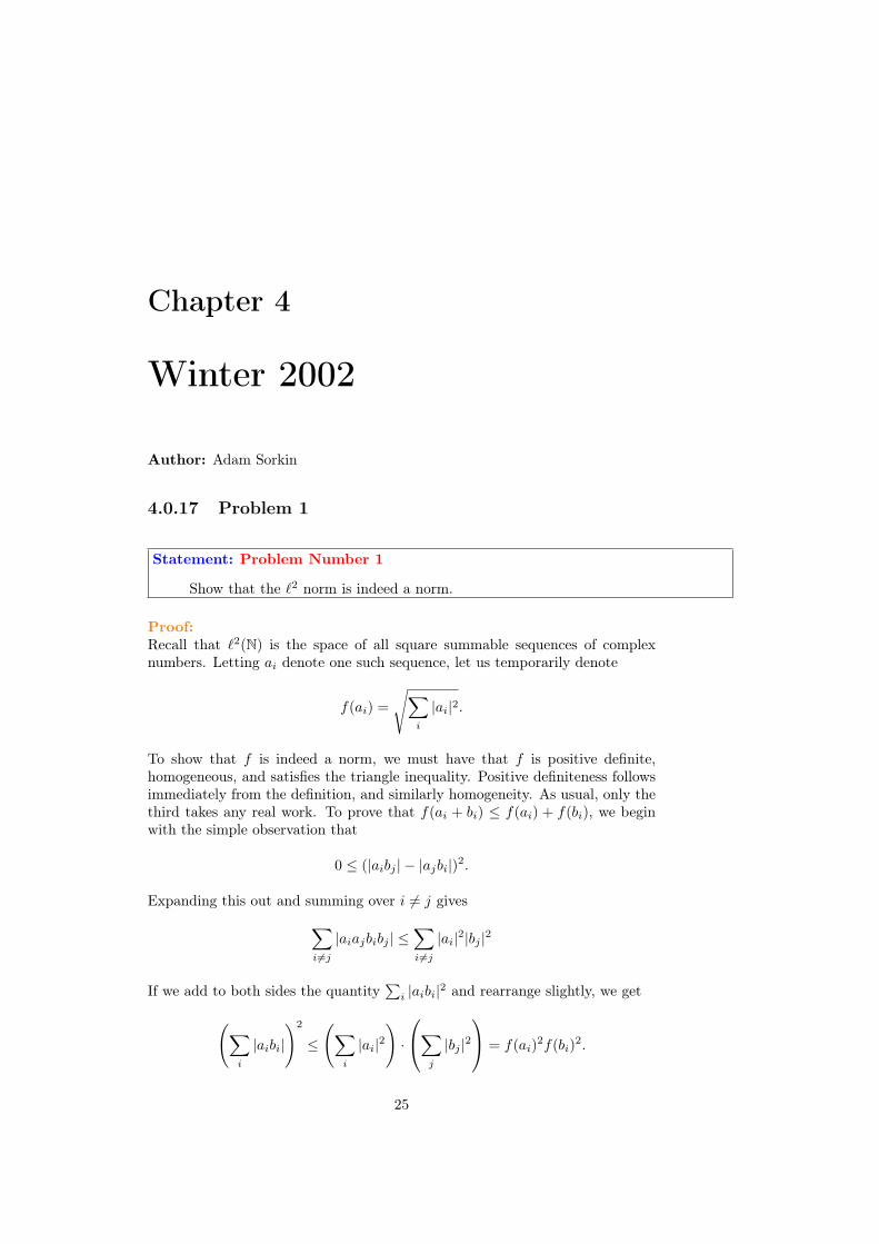
Statement: Problem Number 1
Show that the `2 norm is indeed a norm.
Proof:Recall that `2(N) is the space of all square summable sequences of complexnumbers. Letting ai denote one such sequence, let us temporarily denote
f(ai) =
√∑i
|ai|2.
To show that f is indeed a norm, we must have that f is positive definite,homogeneous, and satisfies the triangle inequality. Positive definiteness followsimmediately from the definition, and similarly homogeneity. As usual, only thethird takes any real work. To prove that f(ai + bi) ≤ f(ai) + f(bi), we beginwith the simple observation that
0 ≤ (|aibj | − |ajbi|)2.
Expanding this out and summing over i 6= j gives∑i 6=j
|aiajbibj | ≤∑i 6=j
|ai|2|bj |2
If we add to both sides the quantity∑i |aibi|2 and rearrange slightly, we get
(∑i
|aibi|
)2
≤
(∑i
|ai|2)·
∑j
|bj |2 = f(ai)
2f(bi)2.
25

Taking roots gives∑i |aibi| ≤ f(ai)f(bi), and using the triangle inequality on
complex numbers gives
f(ai + bi)2 =
∑i
|ai + bi|2
≤∑i
(|ai|2 + |bi|2 + 2|aibi|
)≤ f(ai)
2 + f(bi)2 + 2f(ai)f(bi)
≤ (f(ai) + f(bi))2
Taking roots gives the desired inequality. 2
26

4.0.18 Problem 2
Statement: Problem Number 2
Prove that C([0, 1]), the space of continuous functions on [0, 1], is not completein the L1 metric: ρ(f, g) =
∫|f(x)− g(x)|dx.
Proof:Consider the sequence of functions fn : [0, 1]→ R defined by fn(x) = xn. Clearlythese functions are continuous and integrable, hence in C([0, 1]). Moreover, fnis Cauchy, for we can compute ‖fn‖ = 1/(n+ 1).Now fn has no limit in C([0, 1]), for any L1-limit of fn must be a pointwise limitof fn. But fn converges pointwise to a discontinuous function; specifically it’spointwise limit is zero on [0, 1) and 1 at 1. hence we see 2
27
4.0.19 Problem 3
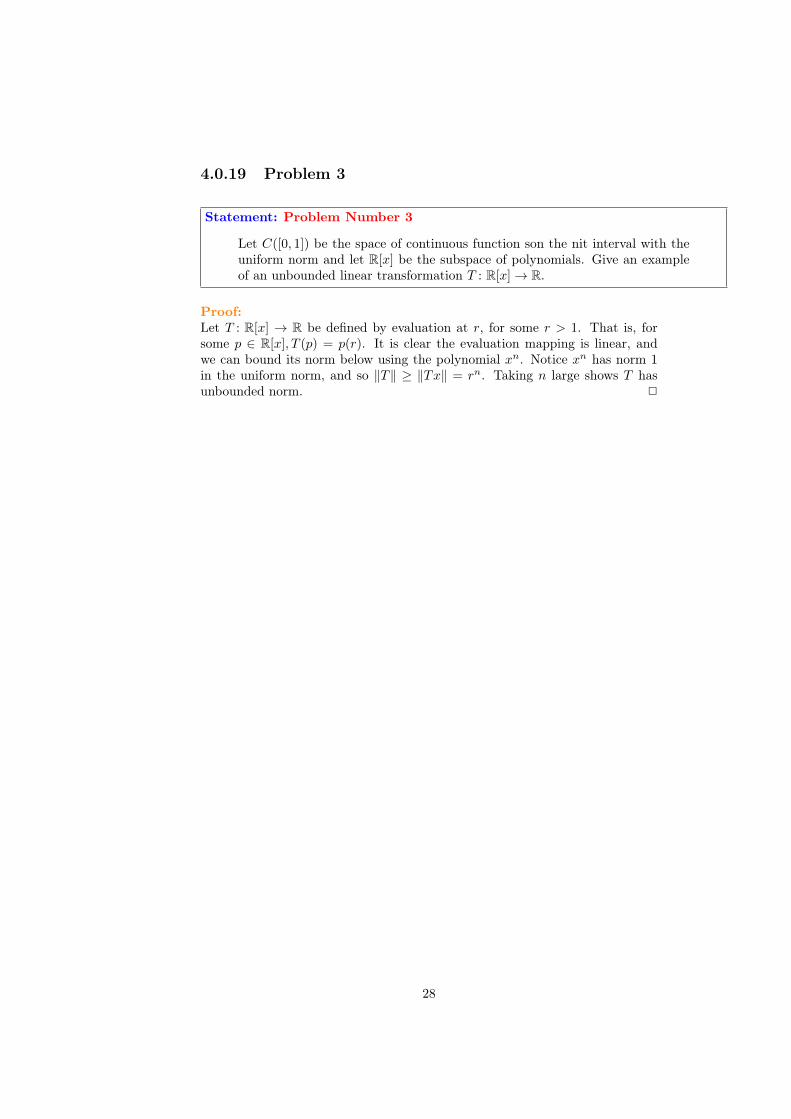
Statement: Problem Number 3
Let C([0, 1]) be the space of continuous function son the nit interval with theuniform norm and let R[x] be the subspace of polynomials. Give an exampleof an unbounded linear transformation T : R[x]→ R.
Proof:Let T : R[x] → R be defined by evaluation at r, for some r > 1. That is, forsome p ∈ R[x], T (p) = p(r). It is clear the evaluation mapping is linear, andwe can bound its norm below using the polynomial xn. Notice xn has norm 1in the uniform norm, and so ‖T‖ ≥ ‖Tx‖ = rn. Taking n large shows T hasunbounded norm. 2
28

4.0.20 Problem 4
Statement: Problem Number 4
Let X be a metric space. Prove or disprove the following:
(a) If X is compact, then X is complete.
(b) If X is complete, then X is compact.
Proof:The first statement is true; the second false. To see compactness implies com-plete, we use the sequential characterization of compactness. Now let xn be aCauchy sequence in X. Then by compactness, xn contains a subsequence xk(n)which converges to some x0 in X. Hence xn → x0, for
|xn − x0| ≤ |xn − xk(n)|+ |xk(n) − x0|.
Therefore xn has a limit in X, and so X is complete. Now complete doesnot imply compact in a metric space. A familiar counterexample is the realnumbers, which are certainly not compact, and are complete (though we do notprove this). 2
29

4.0.21 Problem 5
Statement: Problem Number 5
Let H be a Hilbert space and V a linear subspace. Show that V ⊥⊥ = V .
Proof:Recall that V ⊥ is a closed linear space; this follows immediately from the lin-earity and continuity of 〈·, ·〉. Next recall there is a direct sum orthogonaldecomposition of the Hilbert space H = V ⊥ ⊕ V ⊥⊥. Our final observationis that V ⊥ = (V )⊥; again this follows directly from properties of the innerproduct. Thus we have H = V ⊕ (V )⊥ = V ⊕ V ⊥. Then the isomorphismV ⊥ ⊕ V ∼= V ⊥ ⊕ V ⊥⊥ gives the equality V = V ⊥⊥. 2
30

4.0.22 Problem 6
Statement: Problem Number 6
State Jensen’s inequality. Show that the function ϕ : x → log(1/x) is convex.Suppose that ai ≥ 0 and pi > 0 such that the pi sum to 1. Prove that
ap11 · · · apnn ≤ a1p1 + · · ·+ anpn.
Proof:Jensen’s inequality is as follows. Let (X,µ) be a finite measure space, withΩ =
∫X
1µ < ∞. Let f : X → R be integrable, and ϕ : R → R a convexfunction. Then
ϕ(1
Ω
∫X
fdµ) ≤ 1
Ω
∫X
ϕ fdµ
To see that ϕ : (0,∞) → R as defined above is convex, notice it is twicedifferentiable. Then as ϕ
′′= 1/x2 > 0, it is a convex function.
Finally, consider the measure space X = pi with measure∫Xfdµ =∑
f(pi)pi. Let ϕ be as defined above, and notice the function f : X → Rdefined by f(pi) = ai is integrable. From Jensen’s inequality we get
− log(∑i
aipi) ≤∑i
−pi log ai.
Exponentiating both sides gives the desired inequality. 2
31

Chapter 5
Winter 2005
Author: Jeffrey Anderson
5.0.23 Problem 1
Statement: Problem 1
Show that the mapping T : R→ R defined by
T (x) =π
2+ x− arctan(x)
has no fixed points in R and that
|T (x)− T (y)| ≤ |x− y| for all distinct x, y ∈ R
Why does this example not contradict the contraction mapping theorem?
Proof:Suppose hoping for contradiction that there exists a fixed point for the mapT : R→ R. Then, by definition of fixed point, there is some x ∈ R such that
T (x) = x
⇒T (x) =π
2+ x− arctan(x) = x
⇒π
2− arctan(x) = x− x
⇒ arctan(x) =π
2
Then, under our assumption, we have that their exists some x ∈ R such that
tan(π
2) = x
This is not possible, since tan is not defined at π2 .
Now, let us consider
|T (x)− T (y)|
32

for any two distinct x, y ∈ R. Without loss of generality assume that x < y.We know by the mean value theorem, we have there exists some z ∈ (x, y) suchthat
‖T (x)− T (y)‖ = T ′(z)|x− y|
Then, we also have that for any x ∈ R
T ′(x) =d
dx
(π2
+ x− arctan(x))
= 0 + 1− 1
1 + x2
We can then bound T ′(z) < 1 since 11+z2 ≥ 0. We conclude that
|T (x)− T (y)| = T ′(z)|x− y|< 1|x− y|= |x− y|
This proves the second part of our claim.To substantiate the last claim of this problem, consider the statement of
the Contraction mapping theorem. In the mapping defined above, there is noc ∈ (0, 1) such that
|T (x)− T (y)| < c|x− y|
for all x, y ∈ R.Assume, hoping for contradiction, that the exists a c ∈ (0, 1) such that
|T (x)− T (y)| < c|x− y|
(ie assume that the antecedents of the contraction mapping theorem hold). Weknow by the Mean Value Theorem taught in Math 21A here at UC Davis, forall x, y ∈ R, there exists some ξ ∈ R such that
|T (x)− T (y)| = T ′(ξ)|x− y|
= 1− 1
1 + ξ2︸ ︷︷ ︸T ′(ξ)
|x− y|
We will explicitly exhibit a pair (x, y) which defies this inequality, thus leadingto a contradiction and proving that no such c can exist. Let y = 0. Then wehave
|T (x)− T (0)| =∣∣∣T (x)− π
2
∣∣∣=∣∣∣π2
+ x− arctan(x)− π
2
∣∣∣= |x− arctan(x)|
33

We note that for x > 0 we have x − arctan(x) > x − π2 by the properties of
arctan(x). Now choose
x =π
2(1− c)
We note that π2(1−c) > 0π/2. Then we have
|T (x)− T (0)| = |x− arctan(x)|
> x− π
2
=π
2(1− c)− π
2
=πc)
2(1− c)= cx
Then, given we have a c, we have found a pair (x, y) of points that defies thebound. This contradicts the assumption that our function T above satisfies thecontraction mapping theorem. With this, we have shown each of the three partsof this problem. 2
34

5.0.24 Problem 2
Statement: Problem 2
Prove that the vector space C([a, b]) is seperable. Here and below, C([a, b])is the vector space of continuous functions f : [a, b] → R with the supremumnorm.
Proof:
This is exactly what we wanted to show. 2
35

5.0.25 Problem 3
Statement: Problem 3
Suppose that fn ∈ C([a, b]) is a sequence of functions converging uniformly toa function f . Show that
limn→∞
b∫a
fn(x)dx =
b∫a
f(x)dx
Give a counterexample to show that the pointwise convergence of continuousfunctions fn to a continuous function f does not imply convergence of thecorresponding integrals.
Proof:Let fn ∈ C([a, b]) be a sequence of functions converging uniformly to a functionf . Let ε > 0. Since fn converges uniformly, we have that there is an N ∈ Nsuch that for all n ≥ N
|fn(x)− f(x)| < ε
b− a
for all x ∈ [a, b]. Assuming n ≥ N , we have∣∣∣∣∣∣b∫a
fn(x)dx−b∫a
f(x)dx
∣∣∣∣∣∣ =
∣∣∣∣∣∣b∫a
(fn(x)− f(x))dx
∣∣∣∣∣∣ by linearity of the integral
≤b∫a
|fn(x)− f(x)|dx bringing absolute value inside integral
<
b∫a
ε(b− a)dx by assumption on n
=ε
b− a
b∫a
1dx
=ε
b− a(b− a)
= ε
This proves the first part of our problem. For the second part of this problem,consider the sequence fn ∈ C([0, 1]) which linearly interpolates the followingsecquence of points
• for x ∈ (0, 1/2n), fn is defined by the line through the points (0, 0) and(1/2n, 2n)
• for x ∈ (1/2n, 1/2n−1), fn is defined by the line through the points(1/2n, 2n) and (1/2n−1, 0)
36

• for x ∈ (1/2n−1, 0), fn is defined by the constant function 0.
To explicitly formulate this sequence of functions, we rely on the following:Given two points (x1, y1) and (x2, y2) we can define the interpolating line bycomputing
m =y2 − y1x2 − x1
(y − y1) = m(x− x1)
Then, this sequence of function is defined by
fn(x) =
22nx if 0 ≤ x < 2−n
−22n(x− 1/2n) + 2n if 2−n ≤ x < 2−(n−1)
0 if 2−(n−1) ≤ x ≤ 1
We notice that this sequence of functions converges pointwise to zero, yet theintegral of each fn is one. This demonstrates exactly what we would like. 2
37

5.0.26 Problem 4
Statement: Problem 4
Let l2(Z) denote the complex Hilbert space of sequences xn ∈ C, n ∈ Z suchthat
∞∑n=−∞
|xn|2 <∞
Define the shift operator S : l2(Z)→ l2(Z) by
S((xn)) = (xn+1)
Show that S has no eigenvalues.
Proof:Let xn ∈ `2(Z) as described above. Assume, hoping for contradiction, thatthe shift operator does have an eigenvalue λ ∈ C. By definition we have thefollowing equalities:
S((x0)) = x0+1 = x1 = λx0
S((x1)) = x1+1 = x2 = λx1 = λ2x0
S((x2)) = x2+1 = x3 = λx2 = λ3x0
With this initial observation, we see that the assumption that λ ∈ C is an eigen-value immediately mandates a very unique structure to the sequence xn∞n=−∞.Specifically, assume that n is a positive integer. Then
xn = λnx0
Similarly if m is a negative integer, then
xm = λmx0
Without loss of generality, we can assume |x0| = 1 (if not, we know that thesequence convergence and hence we can use the constant multiple rule for con-verging sequences taught in Math 21C here at UC Davis and normalize to enforcethis condition).
Then we have∞∑−∞|xn|2 =
∞∑−∞|λ|2n
The sequence xn∞n=−∞ illustrates that λ = 0 is can never be an eigenvalue.Similarly, if 0 < |λ| < 1 we have that the sum
0∑−∞|λ|2n
38

diverges. Similarly, if |λ| > 1, we know that
∞∑0
|λ|2n
diverges because it fails the test for convergence. Last, if λ = 1, we have that thesum of all ones diverges because it fails the convergence test. We have reacheda contradiction for any λ ∈ C. It must be that S has no eigenvalues.s 2
39

5.0.27 Problem 5
Statement: Problem 5
Consider the initial value problem
u′(t) = |u(t)|α, u(0) = 0
Show that the solution to this problem is unique if α > 1 and not unique if0 ≤ α < 1
Proof (exercise 2.13 in Applied Analysis):Suppose that α > 1. In this case we reference theorem 2.26 of Applied Analysis.We must check that the antecedents of this theorem are preserved:
In this case, let us define
f(t, u) = u′(t) = |u(t)|α
We note that this function is continuous on the rectangle
R = |t| < T, |u| < L
With this, we see that f is Lipschitz and we get that the solution of our IVP isunique.
Let 0 ≤ α < 1. We will validate the second claim by direct computation.Specifically, we find that
u(t) =
0 t ≤ a(a− α)
11−α (t− α)
11−α t ≥ a
where a is some constant. We also note that u(t) = 0 is a solution to the sameinitial value problem. We have explicitly listed two seperate solutions and thushave shown our second desired property.
Suppose that α > 1. In this case We see that This is exactly what we wantedto show. 2
40

5.0.28 Problem 6
Statement: Problem 6
Let H be a Hilbert Space, H0 a dense linear subspace of H, xn∞n=1 ⊂ H andx ∈ H such that
i. there exists M > 0 such that ‖xn‖ ≤M for all n
ii. limn→∞
〈xn, y〉 = 〈x, y〉 for all y ∈ H0
Prove that xn∞n=1 converges in the weak topology of H
Proof: Theorem 8.40 in Applied AnalysisLet all the assumptions in the problem statement hold. Let y ∈ H. Let ε > 0.We want to show that for that
limn→∞
〈xn, y〉 = 〈x, y〉
We can rewrite this in the form
limn→∞
〈xn − x, y〉 = 0
using the definition of the inner product. We will prove our statement in thisform.
Since y ∈ H and H0 is dense in H, we have that there is some χ ∈ H0
such that ‖χ − y‖ < ε (this is an immediate consequence of the definition ofdensity). Since χ ∈ H0, we know by our assumptions above
limn→∞
〈xn, χ〉 = 〈x, χ〉
We can rearrange this using the same ideas as above to see
limn→∞
〈xn − x, χ = 0 (5.1)
We see that there is some postive integer N such that
| 〈xn − x, χ〉 | < ε
for all n > N by the definition of weak convergence.Now let us consider
|〈xn − x, y〉| = |〈xn − x, y − χ+ χ〉|= |〈xn − x, y − χ〉|+ |〈xn − x, χ〉|≤ |〈xn − x, y − χ〉|+ ε using the assumption (5.1)≤ ‖xn − x‖‖χ− y‖+ ε applying Cauchy Schwarz Inequality≤ (‖xn‖+ ‖x‖)‖χ− y‖+ ε by the triangle inequaltiy≤ (M + ‖x‖)‖χ− y‖+ ε since xn is bounded≤ (M + ‖x‖)ε+ ε by choice of χ
This is exactly what we wanted to show. 2
41

Chapter 6
Fall 2007
6.0.29 Problem 1Author: David Renfrew
Statement: Problem 1
Suppose that f : [0, 1]→ R is continuous. Prove that
limn→∞
∫ 1
0
f(xn)dx
exists and evaluate the limit. Does the limit alway exist if f is only assumedto be integrable?
Proof:Let g(x) := supx f(x), because f is continuous this exist and g is integrablewith f(x) ≤ g(x) so we can apply the LDCT:
limn→∞
∫ 1
0
f(xn)dx =
∫ 1
0
limn→∞
f(xn)dx =
∫ 1
0
f( limn→∞
xn)dx = f(0)
The limit does not necessiarly exist if f is only integrable.Consider f(x) = x−1/2 which is integrable but∫ 1
0
f(xn)dx =
∫ 1
0
x−n/2dx =
(1
1− n/2
)x1−n/2
∣∣∣10
This integral does not converge for n > 1.
This establishes our claim 2
42
6.0.30 Problem 2Author: David Renfrew
6.0.31 Problem 1Author: David Renfrew
Statement: Problem 2
Suppose that for each n ∈ Z, we are given a real number ωn. For each t ∈ R,define a linear operator T (t) on 2π-periodic function by
T (t)
(∑n∈Z
fneinx
)=∑n∈Z
eiωntfneinx,
where f(x) =∑n∈Z fne
inx with fn ∈ C.(a) Show that T (t) : L2(T)→ L2(T) is a unitary map.(b) Show that T (s)T (t) = T (s+ t) for all s, t ∈ R.(c) Prove that if f ∈ C∞(T), meaning that it has continuous derivative of allorders, then T (t)f ∈ C∞(T).
Proof:(a) First observe by the density of the trig polynomials T (t) is onto.Then let f, g ∈ L2(T).Then compute the inner product using the Fourier coefficients.
〈T (t)f, T (t)g〉 =∑n∈Z
(eiωntfn
) (eiωntgn
)=∑n∈Z
fngn
= 〈f, g〉
(b) By direct computation:
T (s)T (t)f = T (s)∑n∈Z
eiωntfneinx
=∑n∈Z
eiωnseiωntfneinx
=∑n∈Z
eiωns+tfneinx
= T (s+ t)f
(c) This follows by Sobolev embedding.
43
6.0.32 Problem 3Author: David Renfrew
Statement: Problem 3
Let (X, ‖ · ‖X), (Y, ‖ · ‖Y ), (Z, ‖ · ‖Z) be Banach spaces, with X compactlyimbedded in Y , and Y continuously imbedded in Z (meaning: X ⊂ Y ⊂ Z;bounded sets in (X, ‖·‖X) are precompact in (Y, ‖·‖Y ); and there is a constantM such that ‖x‖Z ≤ M‖x‖Y for every x ∈ Y ). Prove that for every ε > 0there exists a constant C(ε) such that
‖x‖Y ≤ ε‖x‖X + C(ε)‖x‖Z for every x ∈ X.
Proof:Assume for contradiction that there is an ε for which such a C(ε) does not exist.Then there exist a sequence xn with X-norm 1 such that
‖xn‖Y > ε+ n‖xn‖Z
By the compact embedding the xn’s have a convergent subsequence in the Ynorm, let us pass to this subsequence.This means ‖xn‖Y will converge to a constant, but this means the above in-equality will only be preserved if ‖xn‖Z goes to zero.This implies xn → 0 in all spaces. This contradicts the assumption that‖xn‖Y > ε, so the desired inequality is proved.
44

6.0.33 Problem 4Author: David Renfrew
Statement: Problem 4
Let H be the weighted L2-space
H =
f : R→ C
∣∣∣∣∣∫R
e−|x||f(x)|2dx <∞
with inner product
〈f, g〉 =
∫Re−|x|f(x)g(x)dx.
Let T : H → H be the translation operator
(Tf)(x) = f(x+ 1).
Compute the adjoint T ∗ and the operator norm ‖T‖.
Proof:First the adjoint computation: Let f, g ∈ H.
〈Tf, g〉 =
∫Re−|x|Tf(x)g(x)dx
=
∫Re−|x|f(x+ 1)g(x)dx
=
∫Re−|x−1|f(x)g(x− 1)dx
=
∫Re−|x|f(x)e|x|−|x−1|g(x− 1)dx
= 〈f, e|x|−|x−1|g(x− 1)〉
So T ∗ g(x) = e|x|−|x−1|g(x− 1).
Now we compute the norm:
45

6.0.34 Problem 5Author: David Renfrew
Statement: Problem 5
a) State the Rellich Compactness Theorem for the space W 1,p(Ω) for Ω ⊂ Rn.(b) Suppose that fn∞n=1 is a bounded seqeunce in H1(Ω) for Ω ⊂ R3 open,bounded, and smooth. Show that there exists an f ∈ H1(Ω) such that for asubsequence fnl∞l=1,
fnlDfnl fDf weakly in L2(Ω),
where D =(
∂∂x1
, ∂∂x2
, ∂∂x3
)denotes the weak gradient operator.
Proof:
(a) Let Ω ⊂ Rn be an open, bounded Lipschitz domain. Let 1 ≤ p ≤ n andp∗ := np
n−p .Then W 1,p(Ω) is compacted embedded in Lq(Ω) for all 1 ≤ q < p∗.
(b)Since fn is bounded in H1 so fn and Dfn are bounded in L2.
Bounded sets are weakly precompact so after passing to a subsequence thereexist an f and g such that fn f and Dfn g. Additionally g = Df .
fnDfn = (fn − f)Dfn + fDfn
The Sobolev conjugate p∗ = npn−p = 3∗2
3−2 = 6 > 2, so we can apply Rellich’sTheorem, after passing to a subseqence, to say that fnl → f strongly in L2.Since Dfn are bounded (fn − f)Dfn converges to 0 in L2. So we have:
liml→∞
fnlDfnl = liml→∞
(fnl − f)Dfnl + fDfnl
0 + fDf
As desired.
46

Author: David Renfrew
Statement: Problem 6
Let Ω := B(0, 12 ) ⊂ R2 denote the open ball of radius 12 . For x = (x1, x2) ∈ Ω,
let
u(x1, x2) = x1x2 [log (| log(|x|)|)− log log 2] where |x| =√x21 + x22.
(a) Show that u ∈ C1(Ω).
(b) Show that ∂2u∂x2j∈ C(Ω). for j = 1, 2, but that u 6∈ C2(Ω).
(c) Using the elliptic regularity theorem for the Dirichlet problem on the disc,show that u ∈ H2(Ω).
Proof:
First we compute the derivaties:
∂
∂x1u(x1, x2) = x2 [log (| log(|x|)|)− log log 2] +
x1x2| log(|x|)|
log(|x|)| log(|x|)|
1
|x|x1|x|
∂
∂x2u(x1, x2) = x1 [log (| log(|x|)|)− log log 2] +
x1x2| log(|x|)|
log(|x|)| log(|x|)|
1
|x|x2|x|
47
Chapter 7
Winter 2008
7.0.35 Problem 1Author: Jeffrey Anderson
Statement: Problem Number
Define fn : [0, 1]→ R by
fn(x) = (−1)nxn(1− x)
a. Show that∞∑n=0
fn converges uniformly on [0, 1]
b. Show that∞∑n=0|fn| converges pointwise on [0, 1] but not uniformly
Proof:
48

7.0.36 Problem 2Author: Jeffrey Anderson
49
7.0.37 Problem 3Author: Jeffrey Anderson
Statement: Problem 3
Suppose thatM is a (nonzero) closed linear subspace of a Hilbert space H andφ :M→ C is a bounded linear functional onM. Prove that there is a uniqueextension of φ to a bounded linear function on H with the same norm.
Proof:The first thing to notice is that this problem is known as the Hahn-BanachTheorem for Closed linear subspaces. With this in mind, the way to establishthis result is:
• construct the norm preserving extension explicitly to the larger subspace
• Invoke the axiom of choice to establish that the construction above givesour desired extension
Then, let H be a Hilbert space, letM be a closed linear subspace of H, letφ :M→ C be a bounded linear functional onM. We want to show
i. there exists a norm preserving extension of φ
ii. this extension is unique
First we will show that an extension exists. Let x0 ∈ H such that x0 /∈ M,Let
Y1 = 〈x0,M〉 = spanx0,M
We know that for any y ∈ Y1, we have y = x + λx0 for x ∈ M,λ ∈ C. Let usdefine a mapping Φ : Y1 → C by
Φ(y) = Φ(x+ λx0)
= φ(x) + λα
for some α ∈ C.We can check that this mapping is linear:
Φ(y + z) = Φ ((x+ λx0) + (w + µw0))
= φ(x+ w) + (λ+ µ)α
= φ(x) + λα+ φ(w) + µα
= Φ(y) + Φ(z)
The trick of this problem is to choose α so that the extended funcitonal hasnorm 1.
Recall by definition
‖Φ‖op = sup‖y‖=1
Φ(y)‖H
= sup‖x+λx0‖=1
‖φ(x) + λα‖C
50

We can bound ‖Φ‖op above by one using the inequalities
‖Φ(y)‖op = ‖φ(x) + λα‖C≤ ‖x+ λx0‖H= ‖y‖H
Now, to find the lower bound, take x = −λx ∈M. Then
|φ(−λx) + λα| = | − λφ(x) + λα|≤ ‖ − λx+ λx0‖H
This is true if and only if
|λ||φ(x)− α| ≤ |λ|‖x− x0‖H⇔ |φ(x)− α| ≤ ‖x− x0‖H
From here, we would like to solve for α such that
− ‖x− x0‖H ≤ φ(x)− α ≤ ‖x− x0‖H⇔− φ(x)− ‖x− x0‖H ≤ −α ≤ −φ(x) + ‖x− x0‖H⇔α ∈ [Φ(x)− ‖x− x0‖,Φ(x)− ‖x− x0‖]
We introduce the notation
Ax = Φ(x)− ‖x− x0‖Bx = Φ(x) + ‖x− x0‖
We also let Σ = [Ax,Bx] ⊂ R. We note that Σ 6= ∅ ⇐⇒ Ax ≤ Bx for allx, y ∈M. We note that
φ(x)− φ(y) = φ(x− y)
= ‖x− y‖= ‖x+ x0 − x0 − y‖≤ ‖x− x0‖+ ‖y − x0‖
Then we have
φ(x)− ‖x− x0‖ ≤ φ(y) + ‖y − x0‖
With this we see there is an extension that perserves the norm. We must nowestablish uniqueness.
51

7.0.38 Problem 4Author: Mohammad Omar
52

7.0.39 Problem 5Author: Jeffrey Anderson
Statement: Problem 5
Let 1 ≤ p < ∞ and let I = (−1, 1) denote the open interval in R. Find thevalues of α as a function of p for which the function |x|α ∈W 1,p(I)
Proof:
We want to find the values of α as a function of p such that (|x|)α ∈W 1,p(I).By the definition of the space W 1,p(I), we know we must solve three relatedproblems. These problems include
(a) Find the values of α in terms of p such that (|x|)α ∈ Lp(I)
(b) Find the values of α in terms of p such that ddx (|x|)α ∈ Lp(I) (where we
are taking the weak derivative here)
(c) Compare these values of α to find the correct interval we desire
First, by the definition of the Lp-norm, we have
‖(|x|)α‖p =
1∫−1
|(|x|)α|pdm
1/p
=
1∫0
xpαdm
1/p
by symmetry of |x| around x = 0
We know by a theorem discussed in Math 21B here at UC Davis∞∫1
xβdm <∞⇔ β ∈ (−1,∞)
From here we notice that there is a relationship between the integrability ofx1/β on (0, 1) and the integrability of xβ on the interval (1,∞).
Then1∫
0
xµdm <∞⇔ µ ∈ (−1, 0) ∪ [0,∞)
We conclude that xpα has finite integral on (0, 1) if and only if pα > −1 orα > −1
pSecond, we have that if the weak derivative of this function exists, it is equal
(almost everywhere) to the classical derivative of our function. We know, bydefinition
(|x|)α =
(−x)α if x < 00 if x = 0xα if x > 0
53

This function is classically differentiable everywhere except x = 0. The classicderivative of this function using methods taught in Math 21A here at UC Davisis given by
d
dx(|x|)α =
−α(−x)α−1 if x < 0
αxα−1 if x > 0
Now we take the Lp norm of the weak derivative ∂(|x|)α:
‖∂(|x|)α‖p =
1∫−1
|α(|x|)α−1|pdm
1/p
= 2α
1∫0
(x)p(α−1)dm
1/p
We conclude
‖∂(|x|)α‖p <∞⇔ p(α− 1) > −1
⇔ α > 1− 1
p
Last, we conclude that the only way that |x|α ∈W 1,p(I) is if α > 1− 1p
54

7.0.40 Problem 6Author: Mohammad Omar
55

Chapter 8
Fall 2008
8.0.41 Problem 1Author: Bailey Meeker
Statement: Problem 1
Prove that the dual space of c0 is `1, where c0 =xn∞n=1| lim
n→∞xn = 0
Proof:We can restate this problem as such: Let T ∈ c∗0. Then there is a an∞n=1 ∈ `1such that T (xn∞n=1) =
∑xnan for all xn∞n=1 ∈ `1.
Let δm,n(x) =
1 : n = m0 : n 6= m
. Let an = T (δn) where δn = (0, 0, . . . , 0, 1, 0, . . .)
with the 1 appearing in the nth coordinate. Let xn∞n=1 ∈ c0. Finally, defineyn∞n=1 by the folowing: yn =
∑nk=1 xkδk.
Step 1: Show that T can be identified with some sequence an.By the definition above,
T (yn) = T
(n∑k=1
xkδk
)=
n∑k=1
T (xkδk) =
n∑k=1
xkT (δk) =
n∑k=1
xkak.
Note that∑nk=1 T (xkδk) =
∑nk=1 xkT (δk) since T is a bounded linear functional
on c0, and thus scalar multiples come through. Consider
yn − xn∞n=1 =
n∑k=1
xkδk − xn∞n=1 = (x1, x2, . . . , xn, 0, . . .)− xn∞n=1
= (x1, x2, . . . , xn, 0, . . .)− xn∞n=1 = (0, . . . , 0,−xn+1,−xn+2, . . .).
Then consider the c0 norm of this difference:
‖yn − xn∞n=1‖c0 = lub |yn − xn∞n=1| = lub|xk| |k ≥ n.
Then if we take the limit as n→∞ we see that
limn→∞ ‖yn − xn∞n=1‖c0 = limn→∞lub|xk| |k ≥ n = limsupn→∞xn∞n=1 = limn→∞xn = 0.
56

Therefore limn→∞yn = xn∞n=1 in c0. We assumed that T is a bounded linearfunctional, therefore T is continuous. Then
T (xn∞n=1) = T (limn→∞yn) = limn→∞T (yn) = limn→∞
n∑k=1
xkak =
∞∑k=1
xkak.
Step 2: Show that the sequence an∞n=1 ∈ `1.To prove this, we will use the fllowing sequence: γm,n∞m=1 where
γm,n =
1 m ≤ n and am ≥ 00 m ≤ n and am < 00 m > n
Consider
T (γm,n∞m=1) =
n∑k=1
γk,nak =
n∑k=1
|ak|
by construction. We know that γm,n∞m=1 ∈ c0 since γm,n = 0 for all n > m.Specifically we note that ‖γm,n‖c0 = 1 by construction.
2
57

8.0.42 Problem 2Author: Mohamed Omar
Statement: Problem 2
Let fn∞n=1 be a sequence of differentiable functions on a finite interval [a, b]such that the function themselves and their derivatives are uniformly boundedon [a, b]. Prove that fn∞n=1 has a uniformly converging subsequence.
Proof:
Since [a, b] is a compact subset of R, the Arzela-Ascoli Theorem implies thatfn ⊂ C([a, b]) has a uniformly convergent subsequence if we can prove itis both uniformly bounded and equicontinuous. We are given that fn isuniformly bounded, so it suffices to show it is equicontinuous. We prove thestronger result that the fn is uniformly equicontinuous.
Since f ′n are uniformly bounded, there is a constant C > 0 such that|f ′n(x)| ≤ C for all n and for all x ∈ [a, b]. Now let ε > 0, fn and x, y ∈ [a, b] bearbitrary and such that |x− y| < ε
C. By the Mean Value Theorem, there exists
c ∈ (x, y) such that f ′n(c) =fn(x)− fn(y)
x− y. From this we have
|fn(x)− fn(y)| = |f ′n(c)||x− y| < C( εC
)= ε.
This argument is independent of our choice of x, y and n, so we conclude fnis uniformly equicontinuous. 2
58
8.0.43 Problem 3Author: Mohamed Omar
Statement: Problem 3
Let f ∈ L1(R) and Vf be the closed subspace generatred by the translates off : f(· − y)|∀y ∈ R. Suppose f(ξ0) = 0 for some ξ0. Show that h(ξ0) = 0 forall h ∈ Vf . Show that if Vf = L1(R), then f never vanishes.
Proof:
Recall that, upto scaling,
f(ξ0) =
∫Rf(x)e−2πixξ0 dx.
Now suppose f(ξ0) = 0. Then for any h = f(· − y) for y ∈ R, we have
h(ξ0) =
∫Rf(x− y)e−2πixξ0 dx
=
∫Rf(x)e−2πi(x+y)ξ0 dx
= e−2πiyξ0∫Rf(x)e−2πixξ0 dx
= e−2πiyξ0 f(ξ0)
= 0.
Let Wf be the linear space spanned by functions h = f(· − y) for y ∈ R. Sincethe Fourier Transform is linear, it follows h(ξ0) = 0 for all h ∈ Wf . Now anyfunction h ∈ Vf is either in Wf (in which case we just showed h(ξ0) = 0),or is the L1 limit of functions hn ∈ Wf , in which case h(ξ) = 0 because L1
convergence implies pointwise convergence. 2
59

8.0.44 Problem 4Author: Mohamed Omar
Statement: Problem 4
a. State the Stone-Weierstrass theorem for a compact Hausdorff space X.
b. Prove that the algevra generated by function so the form
f(x, y) = g(x)h(y)
where g, h ∈ C(X) is dense in C(X ×X).
Proof:
[a.] Let X be a compact Hausdorff space, and A be a subalgebra of C(X)which contains a non-zero constant function, and separates points (i.e. for allx1, x2 ∈ X, there exists f ∈ C(X) such that f(x1) 6= f(x2)). Then A is densein C(X).
[b.] First note that if X is a compact Hausdorff space, then so is X×X. LetA be the algebra generated by functions of the form g(x)h(y) where g, h ∈ C(X).Since for any pair g, h ∈ C(X) we have g(x)h(y) ∈ C(X×X), A is a subalgebraof C(X × X). The constant function g(x, y) = 1 for all (x, y) ∈ X × X isa member of A since it is the product of the constant function g(x) = 1 anditself. By the Stone-Weierstrass Theorem it suffices to show that A separatespoints. Let (x1, y1), (x2, y2) ∈ X ×X be different points. Then at least one ofthe following is true: x1 6= x2 or y1 6= y2. Assume without loss of generalitythat x1 6= x2. Since X is Hausdorff, there is an open set U containing x1 thatdoes not contain x2. By Urysohn’s Lemma, there is a function g ∈ C(X) thatis 1 on U and 0 otherwise. This g, together with the constant function h = 1 onX, gives the function gh ∈ C(X ×X) that separates (x1, y1) and (x2, y2) (sincegh(x1, y1) = 1 and gh(x2, y2) = 0). 2
60

8.0.45 Problem 5Author: Mohamed Omar
Statement: Problem 5
For r > 0, define the dilation drf : R → R of the function f : R → R bydrf(x) = f(rx) and the dialation drT of the distribution R ∈ D′(R) by
〈drT, φ〉 =1
r
⟨T, d1/rφ
⟩for all test functions φ ∈ D(R).
• Show that the dialation of a regular distribution Tf , given by
〈Tf , φ〉 =
∫f(x)φ(x)dx
agrees with the dilation of the corresponding function f
• A distribution is homogeneous of degree n if drT = rnT . Show that theδ−distribution is homogeneous of degree −1
• IF T is a homogeneous distribution of degree n, prove that the derivativeT ′ is a homogeneous distribution of degree n− 1.
Proof:
[a.] Let φ ∈ D(R) be arbitrary. We have
〈drTf , φ〉 =1
r〈Tf , d1/rφ〉
=1
r
∫f(x)φ
(xr
)dx
=
∫f(rx)φ(x) dx
= 〈Trf , φ〉
Since φ is arbitrary, we conclude drTf = Trf .
[b.] Let φ ∈ D(R) be arbitrary. We have
〈drδ, φ〉 =1
r〈δ, d1/rφ〉
=1
rφ(r · 0) (by definition of δ)
=1
rφ(0)
= 〈1rδ, φ〉
Since φ is arbitrary, we conclude drδ = 1r δ and hence δ is homogeneous of degree
-1.
61

[c.] Let T ′ be the derivative of a distribution T . Let φ ∈ D(R) be arbitrary.Assume that T is homogeneous of degree n. We have
〈drT ′, φ〉 =1
r〈T ′, d1/rφ〉
= −1
r〈T, (d1/rφ)′〉
= −1
r〈T, 1
rd1/r(φ
′)〉
= − 1
r2〈T, d1/r(φ′)〉
= − 1
r2〈T, d1/rφ′〉
= −1
r〈drT, φ′〉
= −1
r〈rnT, φ′〉 (since T has degree n)
= rn−1 (−〈T, φ′〉)= 〈rn−1T ′, φ〉.
Since φ is arbitrary, it follows drT ′ = rn−1T and hence T ′ is homogeneous ofdegree n− 1.
62

8.0.46 Problem 6Author: Mohamed Omar
Statement: Problem 6
Calculus of variations.
Proof:
63

Chapter 9
Winter 2009
Author: Ricky Kwok
9.0.47 Problem 1
Statement: Problem 1
Let 1 < p < 2.
(a) Given an example of a function f ∈ L1(R) such that f /∈ Lp(R) and afunction g ∈ L2(R) such that g /∈ Lp(R).
(b) If f ∈ L1(R) ∩ L2(R), prove that f ∈ Lp(R).
Proof:Let f(x) = x−1/pχ(0,1). Then
||f ||1 = limε→0
∫ 1
ε
x−1/p dx =x1−1/p
1− 1/p
∣∣∣10
=p
p− 1<∞.
However,
||f ||pp = limε→0
∫ 1
ε
x−1 dx = limε→0
ln(x)∣∣∣1ε
= − limε→0
log(ε) =∞.
Hence f ∈ L1, but f /∈ Lp.
Let g(x) = x−1/pχ(1,∞). Since p < 2, we have 1/p > 1/2, or 2/p > 1, so that1− 2/p < 0.
||g||2 =
∫ ∞1
x−2/p dx =x1−2/p
1− 2/p
∣∣∣∞1
= limx→∞
x1−2/p
1− 2/p− 1
1− 2/p=
p
p− 2.
However,
||g||pp =
∫ ∞1
x−1 dx =∞.
64

Thus, g ∈ L2, but g /∈ Lp.
Now suppose f ∈ L1 ∩ L2. Define
A = x ∈ R : |f(x)| > 1.
Then we have
||f ||pp =
∫R|f(x)|p dx
=
∫A
|f(x)|p dx+
∫Ac|f(x)|p dx
≤∫A
|f(x)|2 dx+
∫Ac|f(x)|1 dx ≤ ||f ||22 + ||f ||11
Therefore, if f ∈ L1 and f ∈ L2, then f ∈ Lp(R). 2
65

9.0.48 Problem 2
Statement: Problem 2
(a) State the Weierstrass approximation theorem.
(b) Suppose that f : [0, 1]→ R is continuous and∫ 1
0
xnf(x) dx = 0
for all nonnegative integers n. Prove that f = 0.
Proof:
TheWeierstrass approximation theorem states that for a closed interval [a, b],the space of continuous functions on this interval C([a, b]) can be uniformlyapproximated with polynomials, i.e. there exists a sequence (fm) ∈ Π([a, b])such that
limm→∞
||fm − f ||unif = limm→∞
supx∈[a,b]
|fm(x)− f(x)| = 0,
where Π([a, b]) is the space of polynomials with domain [a, b].
Since f is continuous over [0, 1], we can take a sequence of polynomials(fm) : [0, 1] → R to approximate f uniformly. Then we can pass limit underthe integral sign (see Exercise 2.2).
limm→∞
∫ 1
0
|fm(x)f(x)−f(x)f(x)| dx ≤∫ 1
0
limm→∞
|fm(x)−f(x)||f(x)| dx ≤ limm→∞
||fm−f ||unif∫ 1
0
|f(x)| dx.
This shows∫ 1
0f(x)2 dx = 0. Since (f(x))2 ≥ 0 for all x, and f is continuous,
f(x) = 0 for all x, i.e. f ≡ 0. 2
66

9.0.49 Problem 3
Statement: Problem 3
(a) Define strong convergence, xn → x, and weak convergence, xn x, of asequence (xn) in a Hilbert space H.
(b) If xn x weakly in H and ||xn|| → ||x||, prove that xn → x strongly.
(c) Give an example of a Hilbert space H and a sequence (xn) in H such thatxn x weakly and
||x|| < lim infn→∞
||xn||.
Proof:
(a) Let || · || denote the norm in the Hilbert space. Strong convergence is
limn→∞
||xn − x|| = 0.
Let (·, ·) denote the inner product in the Hilbert space. Weak convergenceis
limn→∞
(xn, y) = (x, y) ∀y ∈ H.
(b) Suppose xn x and ||xn|| → ||x||. Then ||xn||2 → ||x|| and (xn, x) →(x, x) = ||x||2 and (x, xn) = (xn, x)→ (x, x) = ||x||2 since x ∈ H,
||xn − x||2 = (xn − x, xn − x) = (xn, xn)− (xn, x)− (x, xn) + (x, x)
→ ||x||2 − ||x||2 − ||x||2 + ||x||2 = 0.
Hence, ||xn − x||2 → 0, therefore ||xn − x|| → 0.
(c) Let H = L2(R), be the set of all square-integrable functions on the realline. Define the sequence gn = χ(n,n+1) denote the characteristic functionon the intervals (n, n+ 1). Then we have for every n ∈ N,
||gn|| =∫ n+1
n
12 dx = 1.
I claim gn 0. To see this, let f ∈ L2(R). Then
||f ||22 =
∫ ∞−∞|f(x)| dx =
∞∑n=−∞
∫ n+1
n
|f(x)|2 dx.
Now, Bessel’s inequality states that
67

limn→±∞
∫ n+1
n
|f(x)|2 dx = 0
Then the inner product of gn with f is given by
(gn, f) =
∫ n+1
n
f(x) dx =: yn.
Notice that by Jensen’s inequality,
∫ n+1
n
|f(x)|2 dx ≥(∫ n+1
n
f(x) dx)2
.
So we have∫ n+1
nf(x) dx→ 0 as n→∞. Therefore,
(gn, f)→ 0 ⇒ gn 0.
Then ||0|| = 0 < 1 = lim infn→∞ ||gn||. Therefore gn = χ(n,n+1) satisfiesthe weak convergence to 0 and ||0|| < lim infn→∞ ||gn|| = 1. 2
68

9.0.50 Problem 4
Statement: Problem 4
Suppose that T : H → H is a bounded linear operator on a complex Hilbertspace H such that
T ∗ = −T, T 2 = −I
and T 6= ±iI. Define
P =1
2(I + iT ), Q =
1
2(I − iT ).
(a) Prove that P,Q are orthogonal projections on H.(b) Determine the spectrum of T , and classify it.
Proof:
(a) Notice
P 2 =1
4(I + iT )(I + iT ) =
1
4(I + iT + iT + i2T 2) =
1
4(2I + 2iT ) = P,
and similarly Q2 = Q. Then for all elements y ∈ H,
(Px, y) =
(x
2+iTx
2, y
)=
1
2(x, y) +
−i2
(Tx, y)
=(x,y
2
)+−i2
(x, T ∗y) =
(x,y
2+−i2T ∗y
)=
(x,
(1
2I +
1
2iT
)y
)= (x, Py),
and similarly (Qx, y) = (x,Qy). Therefore P and Q are orthogonal pro-jections (projections and self-adjoint).
(b) To find the spectrum of T, σ(T ), we first find the resolvent of T, ρ(T ) andthen σ(T ) = C \ ρ(T ).
ρ(T ) = λ ∈ C : λI − T : H → H, is one-to-one and onto .
We use the fact that an operator is one-to-one and onto if and only if itis invertible. So, we must find all values λ such that (λI − T )−1 is well-defined. Using T 2 = −I, we take a guess that (λI − T )−1 = c(λI + T ) forsome c ∈ C. To solve for c,
I = (λI − T )c(λI + T ) = c(λ2I − T 2) = c(λ2 + 1)I.
69

We can see that c = 1λ2+1 . Hence,
(λI − T )−1 =λI + T
1 + λ2.
This operator is well-defined for all values λ ∈ C \ ±i. However, sinceT 6= ±iI, ±i /∈ σ(T ), the resolvent set is consists of all complex numbersρ(T ) = C. Therefore, σ(T ) = ∅. 2
70

9.0.51 Problem 5
Statement: Problem 5
Let S(R) be the Schwartz space of smooth, rapidly decreasing functions f :R→ C. Define an operator H : S(R)→ L2(R) by
(Hf)(ξ) = isgn(ξ)f(ξ) =
if(ξ) if ξ > 0
−if(ξ) if ξ < 0,
where f denotes the Fourier transform of f .
(a) Why is Hf ∈ L2(R) for any f ∈ S(R)?
(b) If f ∈ (R) and Hf ∈ L1(R), show that∫Rf(x) dx = 0.
[Hint: you may want to use the Riemann-Lebesgue Lemma.]
Proof:
(a) The function f is in any Lp space since f is in the Schwartz space. Inparticular, f ∈ L1 ∩ L2, implying the Fourier transform of f is in L2 andPlancherel’s theorem holds:
||f ||2 = ||f ||2.
Notice that the L2 norm of Hf is equal to the L2 norm of f because
∣∣Hf(ξ)∣∣ =
∣∣f(ξ)∣∣ ∀ξ ∈ R.
Combining these two, we have
||Hf ||2 = ||Hf ||2 = ||f ||2 = ||f ||2 <∞.
Therefore, Hf ∈ L2.
(b) Since Hf ∈ L1, then the Riemann-Lebesgue Lemma states that Hf iscontinuous and Hf(ξ)→ 0 as |ξ| → ∞. In particular Hf is continuous at0, so
i · limξ→0+
f(ξ) = limξ→0+
Hf(ξ) = limξ→0−
Hf(ξ) = -i · limξ→0−
f(ξ).
Since the left hand side is equal to the negative of the right hand side,these two must both equal zero. Hence, f(0) = 0. But by the definition ofthe Fourier transform,
71

0 = f(0) =
∫Re2πi0xf(x) dx =
∫Rf(x) dx.
Therefore f has zero integral. 2
72
9.0.52 Problem 6
Statement: Problem 6
Let ∆ denote the Laplace operator in R3.
(a) Prove that
limε→0
∫Bcε
1
|x|∆f(x) dx = 4πf(0), ∀f ∈ S(R3)
where Bcε is the complement of the ball of radius ε centered at the origin.
(b) Find the solution u of the Poisson problem
∆u = 4πf(x), lim|x|→∞
u(x) = 0
for f ∈ S(R3).
Proof:
73

Chapter 10
Fall 2009
10.0.53 Problem 1Author: Owen Lewis
Statement: Problem Number 1
For ε > 0, let ηε denote the family of standard mollfiers on R2. Given u ∈L2(R2), define the function
uε = ηε ∗ u in R2.
Prove thatε‖Duε‖L2 ≤ C‖u‖L2 ,
where the constant C depends on the mollifier, not on u.
Proof:By definition, we have that
uε(x) = ηε ∗ u =
∫R2
ηε(x− y)u(y)dy.
Taking the partial derivative with respect to xi, and utilizing the LebesgueDominated Convergence theorem yields
∂xiuε(x) = ∂xi
∫R2
ηε(x− y)u(y)dy =
∫R2
∂xiηε(x− y)u(y)dy.
Now, by Young’s inequality for convolutions (letting p = 2, q = 1 and r = 2)we have
‖∂xiuε‖L2 ≤ ‖∂xiηε‖L1‖u‖L2 . (10.1)
Now, examining ‖∂xiηε‖L1 , we have
‖∂xiηε‖L1 =
∫R2
|∂xiηε(x)|dx
=
∫R2
∣∣∣∣ 1
ε2∂xiη
(xε
)∣∣∣∣ dx.74
Making the change of variables y = xε , we have that ∂xi = 1
ε∂x1and dx = ε2dy.
Therefore the above expression becomes
1
ε
∫R2
|∂yiη (y)| dy.
Because η ∈ C∞c (R2), there exists a constant C that bounds the above expres-sion. Thus we have
‖∂xiuε‖L2 ≤ C
ε.
Combining this with (10.1), and noting that i is arbitrary gives the result
ε‖Duε‖L2 ≤ C‖u‖L2 .
This is exactly what we wanted to show. 2
75

10.0.54 Problem 2Author: Owen Lewis
Statement: Problem Number
Let B(0, 1) ⊂ R3 denote the unit ball |x| < 1. Prove that u = log |x| ∈H1(B(0, 1)).
Proof:We begin by showing that u ∈ L2(B(0, 1)). We first note that for |x| < 1, then|log (|x|)| ≤ 1
|x| . Therefore, utilizing polar coordinates we have
‖u‖L2(B(0,1)) =
∫B(0,1)
u2dx
=
∫B(0,1)
log2(|x|)dx
≤∫B(0,1)
1
|x|2dx
= C
∫ 1
0
1
r2r2dr
= C.
Therefore, u ∈ L2(B(0, 1)). Now a quick calculation shows that
∂xiu =1
|x|xi|x|,
and thusDu =
x
|x|2.
By definition,
‖Du‖L2L2(B(0,1)) =
∫B(0,1)
Du ·Dudx
=
∫B(0,1)
x · x|x|4
dx
= C
∫ 1
0
r2
r4r2dr
= C.
Therefore Du ∈ L2(B(0, 1)). Combined with the previous result we have thatu ∈ H1(B(0, 1)).This is exactly what we wanted to show. 2
76

10.0.55 Problem 6Author: Owen Lewis
Statement: Problem Number
Prove that a normed linear space is complete if and only if every absolutelysummable sequence is summable.
Proof:First, we assume that our space is complete. Let xn be an absolutely summablesequence. Now define ym =
∑mn=1 xn. We have that
‖ym − yk‖ = ‖k∑
n=m
xn‖ ≤k∑
n=m
‖xn‖.
Because xn is absolutely summable, we know that∑∞n=1 ‖xn‖ = M , and thus
for any ε > 0, we can choose m sufficiently large such thatm∑n=1
xn < ε.
Combined with the previous inequality, this shows that the sequence ym isCauchy. By completeness, it has a limit x. Therefore we have
∞∑n=1
xn = limm→∞
m∑n=1
xn = limm→∞
ym = x.
This shows that every absolutely summable sequence is summable.Now assume that every absolutely summable sequence is summable. Let
xn be a Cauchy sequence. By passing to a subsequence if necessary, we canclaim that ‖xk − xk−1‖ ≤ 2−k. Now define y1 = x1, and yk = xk − xk−1 fork > 1. By definition,
m∑k=1
yk = xm.
Furthermore, by construction∞∑k=1
‖yk‖ =
∞∑k=1
‖xk − xk−1‖ ≤∞∑k=1
2−k <∞.
Thus the sequence yk is absolutely summable. By assumption it is thereforesummable, with limit x. Therefore,
limk→∞
xk =
∞∑k=1
yk = x,
which is to say that the subsequence xk is convergent. However, if any Cauchysequence has a convergent subsequence, then the entire sequence is convergent.Thus, our original Cauchy sequence is convergent, and xn → x. This shows thatthe space is complete, and completes the proof.
77

Chapter 11
Winter 2010
Author: Nathan Hannon
11.0.56 Problem 1
Statement: Problem 1
Let (X, d) be a complete metric space, x ∈ X and r > 0. Set D := x ∈ X :d(x, x) ≤ r, and let f : D → X satisfying
d(f(x), f(y)) ≤ k d(x, y)
for any x, y ∈ D, where k ∈ (0, 1) is a constant.
Prove that if d(x, f(x) ≤ r(1− k) then f admits a unique fixed point.
(Guidelines: Assume the Banach fixed point theorem, also known as the con-traction mapping theorem.)
Proof:Let x ∈ D. Then
d(f(x), x) ≤ d(f(x), f(x)) + d(f(x), x)
≤ k d(x, x) + r(1− k)
≤ rk + r(1− k)
= r.
Hence f(x) ∈ D. Since x was arbitrary, we may write f : D → D, and f satisfiesthe hypotheses of the Banach fixed point theorem. We conclude that f admitsa unique fixed point. 2
78

11.0.57 Problem 2
Statement: Problem 2
Give an example of two normed vector spaces, X and Y , and of a sequenceof operators, Tn∞n=0, Tn ∈ L(X,Y ) (L(X,Y ) is the space of the continuousoperators from X to Y , with the topology induced by the operator norm) suchthat Tn∞n=0 is a Cauchy sequence but it does not converge in L(X,Y ).
(Notice that Y cannot be a Banach space otherwise L(X,Y ) is complete.)
Proof:Let X = R and let Y ⊂ L1([−1, 1]) be the subspace consisting of continuousfunctions. We note that any operator T ∈ L(X,Y ) is determined completely byT (1) and that ‖T‖ = ‖T (1)‖. It therefore suffices to find a Cauchy sequence fnin Y that does not converge in Y .
Let fn = x1
2n+1 ∈ Y . Then fn → sgnx in L1([−1, 1]). Hence (fn) is Cauchyin L1([−1, 1]) and hence in Y . However, because sgnx 6∈ Y , (fn) does notconverge in Y . 2
79

11.0.58 Problem 3
Statement: Problem 3
Let (an) be a sequence of positive numbers such that
∞∑n=1
a3n
converges. Show that∞∑n=1
ann
also converges.
Proof:We note that (an) ∈ `3(N). Furthermore, since
∞∑n=1
1
n32
<∞,
we have(1n
)∈ ` 3
2 (N). By Hölder’s inequality,
∞∑n=1
ann≤ ‖(an)‖3
∥∥∥∥( 1
n
)∥∥∥∥32
< ∞.
This is exactly what we wanted to show. 2
80
11.0.59 Problem 4
Statement: Problem 4
Suppose that h : [0, 1]2 → [0, 1]2 is a continuously differentiable funcion fromthe square to the square with a continuously differentiable inverse h−1. Definean operator T on the Hilbert space L2([0, 1]2) by the formula T (f) = f h.Prove that T is a well-defined bounded operator on this Hilbert space.
Proof:Let u = h(x) and let J(u) denote the Jacobian of x with respect to u. Since hand h−1 are continuously differentiable, J is bounded. Let
M = supu∈[0,1]2
|J(u)|.
We also note that h maps [0, 1]2 to itself. We can use a change of variables toevaluate ‖T (f)‖2:
‖T (f)‖22 =
∫[0,1]2
|(f h)(x)|2 dx
=
∫[0,1]2
|J(u)| |f(u)|2 du
≤∫[0,1]2
M |f(u)|2 du
= M‖f‖22.
Hence‖T (f)‖2 ≤
√M‖f‖2;
i. e., T is well-defined and bounded. 2
81

11.0.60 Problem 5
Statement: Problem 5
Let Hs(R) denote the Sobolev space of order s on the real line R, and let
‖u‖s =
(∫R
(1 + |ξ|2
)s |u(ξ)|2 dξ) 1
2
denote the norm on Hs(R), where u(ξ) = 12π
∫R u(x)e−ixξ dx denotes the
Fourier transform of u.
Suppose that r < s < t, all real, and ε > 0 is given. Show that there exists aconstant C > 0 such that
‖u‖s ≤ ε‖u‖t + C‖u‖r ∀u ∈ Ht(R).
Proof:Let
g(ξ) =(1 + |ξ|2
) 12 .
We note that g is strictly positive.Suppose that u ∈ Ht(R) and define a measure ν on R by
dν = |u(ξ)|2 dξ.
We note that
‖gr‖L2(R,ν) =
(∫R
(1 + |ξ|2
)s |u(ξ)|2 dξ) 1
2
= ‖u‖r.
Similarly, ‖gs‖L2(R,ν) = ‖u‖s and ‖gt‖L2(R,ν) = ‖u‖t.Let
C = εs−rs−t .
We note that C does not depend on the choice of u.Suppose that g(ξ) = y. If y ≥ ε
1s−t , then
ys = ys−tyt
≤ εyt
≤ εyt + Cyr.
Otherwise, y < ε1s−t , and
ys = ys−ryr
< Cyr
≤ εyt + Cyr.
It follows thatg(ξ)s ≤ εg(ξ)t + Cg(ξ)r ∀ξ ∈ R.
82

Using Minkowski’s inequality,
‖gs‖L2(R,ν) ≤ ‖εgt + Cgr‖L2(R,ν)
≤ ε‖gt‖L2(R,ν) + C‖gr‖L2(R,ν)
‖u‖s ≤ ε‖u‖t + C‖u‖r.
This is exactly what we wanted to show. 2
83

11.0.61 Problem 6
Statement: Problem 6
Let f : [0, 1] → R. Show that f is continuous if and only if the graph of f iscompact in R2.
Proof:Denote by G the graph of f in R2. Suppose that f is continuous. Since [0, 1] iscompact, f must be bounded. Hence G is bounded.
Now suppose that (xn, yn) ∈ G and (xn, yn) → (x, y). Then xn → x andyn → y. However, because f is continuous, yn = f(xn)→ f(x). It follows thaty = f(x) and that (x, y) ∈ G. Since this holds for all convergent sequences(xn, yn), G is closed.
By the Heine-Borel theorem, G is compact.Conversely, suppose that G is compact. By the Heine-Borel theorem, G
is closed and bounded. Suppose that xn → x and that f(xn) = yn. Lety = lim inf yn and y′ = lim sup yn. Since G is bounded,−∞ < y < y′ < ∞. Choose subsequences ynk and yn′k such that ynk → y andyn′k → y′.
Then (xnk , ynk) → (x, y) and (xn′k , yn′k) → (x, y′). Since G is closed,(x, y), (x, y′) ∈ G, and it follows that y = y′. We conclude that f(xn) →y = f(x).
Because this holds for all convergent sequences (xn), f is continuous.Therefore, f is continuous if and only if G is compact. 2
84

List of Figures
2.1 ISBN: 0387008926, Price: $34.95, Shields Library QA43 .D382001 Regular Loan . . . . . . . . . . . . . . . . . . . . . . . . . . 7
2.2 ISBN: 0486421740, Price: $22.95, Shields Library QA299.8 .J63 . 82.3 ISBN: 007054235X, Shields Reserves Reserves QA300 .R8 1976 . 92.4 ISBN: 0521709792, Price: $75.00, Shields Library QA403.5 .K36
2007 . . . . . . . . . . . . . . . . . . . . . . . . . . . . . . . . . . 102.5 ISBN: 0070542341, Price: $98.99, Shields Library QA300 .R82
1987 . . . . . . . . . . . . . . . . . . . . . . . . . . . . . . . . . . 112.6 ISBN: 0471317160, Price: $129.99, Shields Library QA300 .F67
1999 . . . . . . . . . . . . . . . . . . . . . . . . . . . . . . . . . . 122.7 ISBN: 0821827839, Price:$35.00, Shields Library QA300.L54 2001 132.8 ISBN: 9810241917, Price: $92.00, Shields Library QA300 .H93
2001 . . . . . . . . . . . . . . . . . . . . . . . . . . . . . . . . . . 142.9 ISBN: 0817630031, Price: $55.10, Shields Library QA312 .C56 . . 152.10 ISBN: 0125850506, Price: $123.21, Phy Sci Engr Library QC20.7.F84
R43 1980 Regular Loan . . . . . . . . . . . . . . . . . . . . . . . 16
85

List of Tables
86