Prénom Nom

Document Analysis:Data Analysis and Clustering

Prof. Rolf Ingold, University of Fribourg

Master course, spring semester 2008

© Prof. Rolf Ingold

2

Outline

Introduction to data clustering Unsupervised learning Background of clustering K-means clustering & Fuzzy k-means Model based clustering Gaussian mixtures Principal Components Analysis

© Prof. Rolf Ingold

3

Introduction to data clustering

Statistically representative datasets may include implicitly valuable semantic information the aim is to group samples into meaningful classes

Various terminologies refer to that principle data clustering, data mining unsupervised learning taxonomy analysis knowledge discovery automatic inference

In this course we address two aspects Clustering : perform unsupervised classification Principal Components Analysis : reduce feature spaces

© Prof. Rolf Ingold

4

Application to document analysis

Data analysis and clustering can potentially be applied at many levels of document analysis at pixel level for foreground/background separation on connected components for segmentation or

character/symbol recognition on blocks for document understanding on entire pages to perform document classification ...

© Prof. Rolf Ingold

5

Unsupervised classification

Unsupervised learning consists of inferring knowledge about classes by using unlabeled training data, i.e. where samples are not

assigned to classes

There are at least five good reasons for performing unsupervised learning no labeled samples are available or ground-truthing is too costly useful preprocessing to produce ground-truthed data the classes are not known a priori for some problems classes are evolving over time useful for studying relevant features

© Prof. Rolf Ingold

6

Background of data clustering (1)

Clusters are formed following different criteria members of a class share same or closely related properties members of class have small distances or large similarities members of a class are clearly distinguishable from members of

other classes

Data clustering can be performed on various data types nominal types (categories) discrete types continuous types time series

© Prof. Rolf Ingold

7

Background of data clustering (2)

Data clustering requires similarity measures various similarity and dissimilarity measures (often in [0,1]) distances (with triangular inequality property)

Feature transformation and normalization is often required

Clusters may be center based : members are close to a representative model chain based : members are close to at least one other member

There is a distinction between hard clustering : each sample is member of exactly one class fuzzy clustering : samples have membership functions

(probabilities) associated to each class

© Prof. Rolf Ingold

8

K-means clustering

k-means clustering is a popular algorithm for unsupervised classification assuming the following information to be available the number of classes c

a set of unlabeled samples x1xn

Classes are modeled by their centers 1c and each sample xk is

assigned to the classes of the nearest center

The algorithm works as follows

initialize the vectors 1c randomly

assign each sample xk to the class that minimizes ||xkm||2

update the centers 1c using

stop when classes do no more change

iik

ki

x

x

© Prof. Rolf Ingold

9

Illustration of k-means algorithm

© Prof. Rolf Ingold

10

Convergence of k-means algorithm

The k-means algorithm always converges to a local minimum depending of the centers' initialization

© Prof. Rolf Ingold

11

Fuzzy k-means

Fuzzy k-means is a generalization taking into account a membership function P*(i|xk) normalized as follows

The clustering method consists in minimizing the following cost (where b is fixed)

the centers are updated using

and the membership functions are updated using

i k

ikb

kiPJ2* )]|([ μxx

kPi

ki 1)|(* x

k

bki

k kb

kij

P

P

)]|([

)]|([*

*

x

xxμ

h

bhk

bik

kiP )1/(1

)1/(1*

)/1(

)/1()|(

μx

μxx

© Prof. Rolf Ingold

12

Model based clustering

In this approach, we assume the following information to be available the number of classes c the a priori probability of each class P(i)

the shape of the feature densities p(x|j,j) with parameter j

a dataset of unlabeled samples {x1,...,xn}, supposed to be

drawn

by selecting the class i with probability P(i)

then, selecting xk according to p(x|j,j)

The goal is to estimate the parameter vector 1ct

© Prof. Rolf Ingold

13

Maximum likelihood estimation

The goal is to estimate that maximizes the likelihood of the set D={x1,...,xn}, that is

Equivalently we can also maximize its logarithm, namely

k

kpDp )|()|( θxθ

k

kpDpl )|(ln)|(ln θxθ

© Prof. Rolf Ingold

14

Maximum likelihood estimation (cont.)

To find the solution, we require the gradient is zero

By assuming that i and j are statistically independent, we can state

By combining with the Bayesian rule

we finally obtain that for i=1, ... ,c the estimation of i must satisfy the

condition

k j

jjjkik

iPp

pl )(),|(

)|(

1θx

θx θθ

k

iikik

ii

pp

Pl ),|(

)|(

)(θx

θx θθ

0),|(ln),|( ** k

iikiki pP θxθx θ

)|(

)(),|(),|(

θx

θxθx

k

iiikki p

PpP

© Prof. Rolf Ingold

15

Maximum likelihood estimation (cont.)

In most cases the equation

can not be solved analytically

Instead an iterative gradient descending approach can be used to avoid convergence to a local minimum, an approximate initial

should be used

0),|(ln),|( ** k

iikiki pP θxθx θ

© Prof. Rolf Ingold

16

Application to Gaussian mixture models

We consider the case where of a mixture of Gaussians where the parameter i, i et P(i) have to be determined

By applying the gradient method we can estimate i, i iteratively

where

kki

k

tikikki

i

kki

kkki

i

kkii

P

P

P

P

Pn

P

),|(

))()(,|(

),|(

),|(

),|(1

)(

**

****

*

**

**

*

***

θx

μxμxθx

θx

xθx

μ

θx

jjjkjjki

iikiiki

jjjjk

iiikki

P

P

Pp

PpP

)()()(exp

)()()(exp

)(),|(

)(),|(),|,(

**1**21

2/1*

**1**21

2/1*

**

****

μxμx

μxμx

θx

θxθx

© Prof. Rolf Ingold

17

Problem with local minimums

Maximum likelihood estimation by the gradient descending method can converge to local minimums

© Prof. Rolf Ingold

18

Conclusion about clustering

Unsupervised learning allows to extract valuable information from unlabeled training data it is very useful in practice analytical approaches are generally not practicable iterative methods may be used, but they sometimes converge to

local minimums sometimes even the number of classes is not known; in such

cases clustering can be performed with several hypothesis and the best solution can be selected by information theory

Clustering does not work well in high dimensions there is an interest to reduce the dimensionality of the feature

space

© Prof. Rolf Ingold

19

Objective of Principle Component Analysis (PCA)

From a Bayesian point of view, the more features are used, more accurate are the classification results

But the higher the dimension of the feature space, more difficult it is to get reliable models

PCA can be seen as a systematic way to reduce the dimensionality of the feature space by minimizing the loss of information

© Prof. Rolf Ingold

20

Center of gravity

Let us consider a set of samples described by their feature vectors {x1,x2,...,xn}

The point that best represents the entire set is x0 minimizing

This point corresponds to the center of gravity

since

2

000 )( k

kJ xxx

kk

k

kk

kk

t

k

kk

kkJ

22

0

2

0

2

0

2

0

2

000

)(

)()(2)(

)()()(

mxmx

mxmxmxmx

mxmxxxx

k

knxm

1

© Prof. Rolf Ingold

21

Projection on a line

The goal is to find the line crossing the center of gravity m that best approximate the sample set {x1,x2,...,xn}

let vector e be the unit vector of its direction; then the equation of the line is x = m+ae where a is a scalar representing the distance of x from m

the optimal solution is given by minimizing the squared error

First, the values for a1,a2,...,an minimizing this function are given

that is ak = et (xk - m) corresponding to the orthogonal projection

kkk

k

tk

kk

kkk

kkkn

aa

aaaaJ

22

22

11

)(2

)()(),,...,(

mxmxe

mxexeme

0)(22),,...,( 11

mxee

kt

kk

n aa

aaJ

© Prof. Rolf Ingold

22

Scatter matrix

The scatter matrix of the set {x1,x2,...,xn} is defined as

it differs from the covariance matrix by a factor n-1

k

tkkS ))(( mxmx

© Prof. Rolf Ingold

23

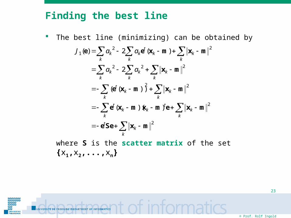
Finding the best line

The best line (minimizing) can be obtained by

where S is the scatter matrix of the set {x1,x2,...,xn}

kk

t

kk

k

tkk

t

kk

kk

t

kk

kk

kk

kkk

k

tk

kk

aa

aaJ

2

2

22

222

221

))((

))((

2

)(2)(

mxSee

mxemxmxe

mxmxe

mx

mxmxee

© Prof. Rolf Ingold

24

Finding the best line (cont.)

To minimize J1(e) we must maximize etSe

using the method of Lagrange multipliers

and by differentiating

we obtain Se = e and etSe = ete =

This means that to maximize etSe we need to select the eigenvector corresponding to the largest eigenvalue of the scatter matrix

)1( eeSeeSee tttu

022

eSee

u

© Prof. Rolf Ingold

25

Generalization to d dimensions

Principal components analysis can be applied for any dimension d up to the dimension of the original feature space each sample is mapped on a hyperplane defined by

the objective function to minimize is

the solution for e is given by the eigenvectors corresponding to the d highest eigenvalues

2

11 )(),,...,(

kk

d

iikind aaaJ xeme

d

iiia

1

emx