preprint series institute of applied mechanics graz university of technology · 2015-10-29 ·...

Institute ofApplied MechanicsInstitut für Baumechanik

Preprint Series

Institute of Applied Mechanics

Graz University of Technology

Preprint No 1/2009

On a reformulated Convolution Quadraturebased Boundary Element Method

Martin SchanzInstitute of Applied Mechanics, Graz University of Technology

Published in: Computer Modeling in Engineering & Sciences, 58(2),109–128, 2010

Latest revision: March 20, 2010

Abstract

Boundary Element formulations in time domain suffer from two problems. First, forhyperbolic problems not too much fundamental solutions are available and, second, thetime stepping procedure is expensive in storage and has stability problems for badly chosentime step sizes. The first problem can be overcome by using the Convolution QuadratureMethod (CQM) for time discretisation. This as well improves the stability. However, stillthe storage requirements are large.A recently published reformulation of the CQM by Banjai and Sauter [Rapid solution ofthe wave equation in unbounded domains, SIAM J. Numer. Anal., 47, 227–249] reducesthe time stepping procedure to the solution of decoupled problems in Laplace domain. Thisnew version of the CQM is applied here to elastodynamics. The storage is reduced tonearly the amount necessary for one calculation in Laplace domain. The properties of theoriginal method concerning stability in time are preserved. Further, the only parameterto be adjusted is still the time step size. The drawback is that the time history of the givenboundary data has to be known in advance. These conclusions are validated by the examplesof an elastodynamic column and a poroelastodynamic half space.

Preprint No 1/2009 Institute of Applied Mechanics

1 Introduction

The Boundary Element Method (BEM) in time domain is especially import to treat wave prop-agation problems in infinite and semi-infinite domains. In this application the main advantageof this method becomes obvious, i.e., its ability to model the Sommerfeld radiation conditioncorrectly. Certainly this is not the only advantage of a time domain BEM but very often themain motivation as, e.g., in earthquake engineering.

The first boundary integral formulation for elastodynamics was published by Cruse and Rizzo[9]. This formulation performs in Laplace domain with a subsequent inverse transformationto time domain to achieve results for the transient behavior. The corresponding formulation inFourier domain, i.e., frequency domain, was presented by Domínguez [11]. The first boundaryelement formulation directly in the time domain was developed by Mansur for the scalar waveequation and for elastodynamics with zero initial conditions [27]. The extension of this for-mulation to non-zero initial conditions was presented by Antes [4]. Detailed information aboutthis procedure may be found in the book of Domínguez [10]. A comparative study of thesepossibilities to treat elastodynamic problems with BEM was given by Manolis [26]. A com-pletely different approach to handle dynamic problems utilizing static fundamental solutions isthe so-called dual reciprocity BEM. This method was introduced by Nardini and Brebbia [30]and details may be found in the monograph of Partridge et al. [31]. A very detailed review onelastodynamic boundary element formulations and a list of applications can be found in twoarticles of Beskos [7, 8].

The above listed methodologies to treat elastodynamic problems with the BEM show mainlythe two ways: direct in time domain or via an inverse transformation in Laplace domain. Mostly,the latter is used, e.g., Ahmad and Manolis [3]. Since all numerical inversion formulas dependon a proper choice of their parameters [29], a direct evaluation in time domain seems to bepreferable. Also, it is more natural to work in the real time domain and observe the phenomenonas it evolves. But, as all time-stepping procedures, such a formulation requires an adequatechoice of the time step size. An improper chosen time step size leads to instabilities or numericaldamping. Four procedures to improve the stability of the classical dynamic time-stepping BEformulation can be quoted: the first employs modified numerical time marching procedures,e.g., [5] for acoustics, [32] for elastodynamics; the second employs a modified fundamentalsolution, e.g., [33] for elastodynamics; the third employs an additional integral equation forvelocities [28]; and the last uses weighting methods, e.g., [42] for elastodynamics and [43] foracoustics.

Beside these improved approaches there exist the possibility to solve the convolution integralin the boundary integral equation with the so-called Convolution Quadrature Method (CQM)proposed by Lubich [21, 22]. Applications to hyperbolic and parabolic integral equations canbe found in [25, 24]. The CQM utilizes the Laplace domain fundamental solution and resultsnot only in a more stable time stepping procedure but also damping effects in case of visco-or poroelasticity can be taken into account (see [37, 38, 34]). The motivation to use the CQMin these engineering applications is that only the Laplace domain fundamental solutions arerequired. This fact is also used for BE formulations in cracked anisotropic elastic [44] or piezo-electric materials [13]. Another aspect is the better stability behavior compared with the abovementioned formulation. For acoustics this may be found in [1, 2] and in elastodynamics in [35].

2


In the framework of fast BE formulations the CQM is used in a Panel-clustering formulation forthe Helmholtz equation by Hackbusch et al. [17]. Recently, some newer mathematical aspectsof the CQM have been published by Lubich [23].

Important for the paper at hand, an essential reformulation of the CQM in case of integralequations has been published by Banjai and Sauter [6]. The proposed formulation transfers thetime stepping procedure to the solution of decoupled Laplace domain problems. The main pa-rameter of the method is still the applied time step size. In this paper, some stability proofs withrespect to the time dependent behavior can be found. Here, this technique is applied to elasto-dynamics for a collocation and a symmetric Galerkin formulation. At the end some numericalstudies are performed concerning the sensitivity on the mesh size, the time step size, and on theprecision of the equation solver. To show the applicability of the reformulated CQM to inelasticBE formulations the displacement results for wave propagation in a poroelastic half space arepresented.

Throughout this paper, vectors and tensors are denoted by bold symbols and matrices by sansserif and upright symbols. The Laplace transform of a function f (t) is denoted by f (s) with thecomplex Laplace parameter s.

2 Boundary integral equation

The hyperbolic partial differential equation to be considered in this work is the elastodynamicsystem, which describes the displacement field u(x, t) of an elastic solid under the assumptionsof linear elasticity. Describing with x and t the position in the three-dimensional Euclidean spaceR3 and the time point from the interval (0,∞) the hyperbolic initial boundary value problem is

c21∇(∇ ·u(x, t))− c2

2∇× (∇×u(x, t)) =∂2u∂t2 (x, t) (x, t) ∈Ω× (0,∞)

u(y, t) = gD(y, t) (y, t) ∈ ΓD× (0,∞)t(y, t) = gN(y, t) (y, t) ∈ ΓN× (0,∞)

u(x,0) =∂u∂t

(x,0) = 0 (x, t) ∈Ω× (0) .

(1)

The material properties of the solid are represented by the wave speeds

c1 =

√E (1−ν)

ρ(1−2ν)(1+ν)c2 =

√E

ρ2(1+ν), (2)

with the material data Young’s modulus E, Poisson’s ration ν, and the mass density ρ. The firststatement in (1) requires the fulfillment of the partial differential equation in the spatial domainΩ for all times 0 < t < ∞. This spatial domain Ω has the boundary Γ which is subdivided into twodisjoint sets ΓD and ΓN at which boundary conditions are prescribed. The Dirichlet boundarycondition is the second statement of (1) and assigns a given datum gD to the displacement u onthe part ΓD of the boundary. Similarly, the Neumann boundary condition is the third statementin which the datum gN is assigned to the surface traction t, which is defined by

t(y, t) = (T u)(y, t) = limΩ3x→y∈Γ

[σ(x, t) ·n(y)] . (3)

3


In (3), σ is the stress tensor depending on the displacement field u according to the strain-displacement relationship and Hooke’s law. For later purposes the traction operator T is defined,which maps the displacement field u to the surface traction t. The boundary conditions have tohold for all times and may be also prescribed in each direction by different types, e.g., rollerbearings. Finally, in the last statement of (1) the condition of a quiescent past is given whichimplies homogeneous initial conditions.

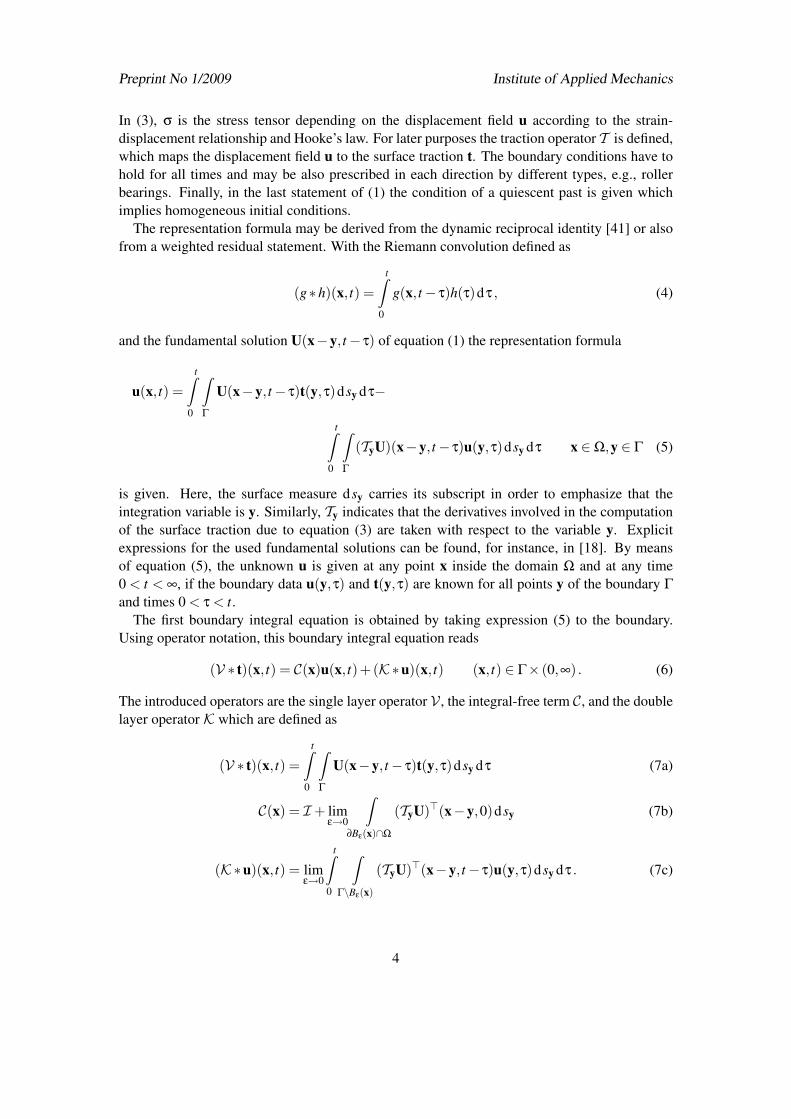
The representation formula may be derived from the dynamic reciprocal identity [41] or alsofrom a weighted residual statement. With the Riemann convolution defined as

(g∗h)(x, t) =tZ

0

g(x, t− τ)h(τ)dτ , (4)

and the fundamental solution U(x−y, t− τ) of equation (1) the representation formula

u(x, t) =tZ

0

ZΓ

U(x−y, t− τ)t(y,τ)dsy dτ−

tZ0

ZΓ

(TyU)(x−y, t− τ)u(y,τ)dsy dτ x ∈Ω,y ∈ Γ (5)

is given. Here, the surface measure dsy carries its subscript in order to emphasize that theintegration variable is y. Similarly, Ty indicates that the derivatives involved in the computationof the surface traction due to equation (3) are taken with respect to the variable y. Explicitexpressions for the used fundamental solutions can be found, for instance, in [18]. By meansof equation (5), the unknown u is given at any point x inside the domain Ω and at any time0 < t < ∞, if the boundary data u(y,τ) and t(y,τ) are known for all points y of the boundary Γ

and times 0 < τ < t.The first boundary integral equation is obtained by taking expression (5) to the boundary.

Using operator notation, this boundary integral equation reads

(V ∗ t)(x, t) = C(x)u(x, t)+(K∗u)(x, t) (x, t) ∈ Γ× (0,∞) . (6)

The introduced operators are the single layer operator V , the integral-free term C, and the doublelayer operator K which are defined as

(V ∗ t)(x, t) =tZ

0

ZΓ

U(x−y, t− τ)t(y,τ)dsy dτ (7a)

C(x) = I+ limε→0

Z∂Bε(x)∩Ω

(TyU)>(x−y,0)dsy (7b)

(K∗u)(x, t) = limε→0

tZ0

ZΓ\Bε(x)

(TyU)>(x−y, t− τ)u(y,τ)dsy dτ . (7c)

4


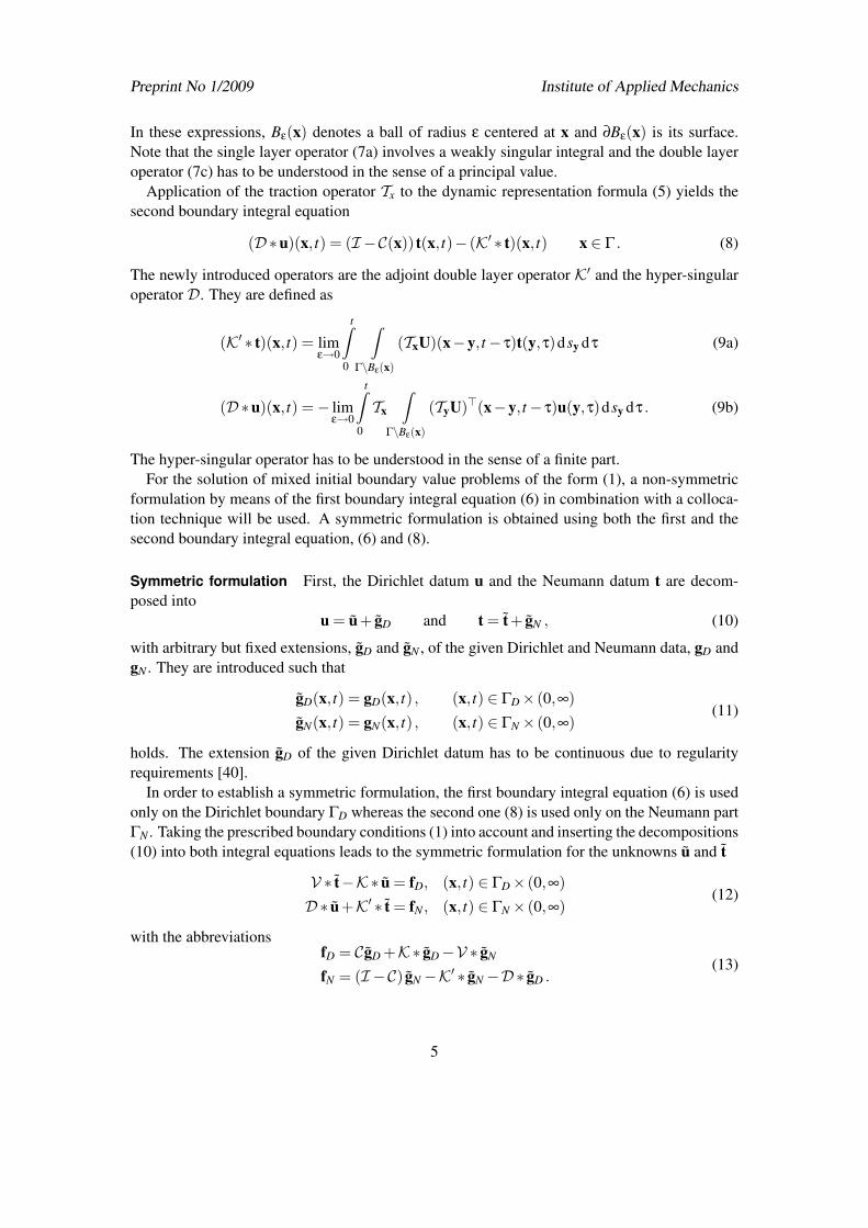
In these expressions, Bε(x) denotes a ball of radius ε centered at x and ∂Bε(x) is its surface.Note that the single layer operator (7a) involves a weakly singular integral and the double layeroperator (7c) has to be understood in the sense of a principal value.

Application of the traction operator Tx to the dynamic representation formula (5) yields thesecond boundary integral equation

(D∗u)(x, t) = (I −C(x)) t(x, t)− (K′ ∗ t)(x, t) x ∈ Γ . (8)

The newly introduced operators are the adjoint double layer operator K′ and the hyper-singularoperator D. They are defined as

(K′ ∗ t)(x, t) = limε→0

tZ0

ZΓ\Bε(x)

(TxU)(x−y, t− τ)t(y,τ)dsy dτ (9a)

(D∗u)(x, t) =− limε→0

tZ0

Tx

ZΓ\Bε(x)

(TyU)>(x−y, t− τ)u(y,τ)dsy dτ . (9b)

The hyper-singular operator has to be understood in the sense of a finite part.For the solution of mixed initial boundary value problems of the form (1), a non-symmetric

formulation by means of the first boundary integral equation (6) in combination with a colloca-tion technique will be used. A symmetric formulation is obtained using both the first and thesecond boundary integral equation, (6) and (8).

Symmetric formulation First, the Dirichlet datum u and the Neumann datum t are decom-posed into

u = u+ gD and t = t+ gN , (10)

with arbitrary but fixed extensions, gD and gN , of the given Dirichlet and Neumann data, gD andgN . They are introduced such that

gD(x, t) = gD(x, t) , (x, t) ∈ ΓD× (0,∞)gN(x, t) = gN(x, t) , (x, t) ∈ ΓN× (0,∞)

(11)

holds. The extension gD of the given Dirichlet datum has to be continuous due to regularityrequirements [40].

In order to establish a symmetric formulation, the first boundary integral equation (6) is usedonly on the Dirichlet boundary ΓD whereas the second one (8) is used only on the Neumann partΓN . Taking the prescribed boundary conditions (1) into account and inserting the decompositions(10) into both integral equations leads to the symmetric formulation for the unknowns u and t

V ∗ t−K∗ u = fD, (x, t) ∈ ΓD× (0,∞)D∗ u+K′ ∗ t = fN , (x, t) ∈ ΓN× (0,∞)

(12)

with the abbreviationsfD = CgD +K∗ gD−V ∗ gN

fN = (I −C) gN−K′ ∗ gN−D∗ gD .(13)

5


3 Boundary element formulation

A boundary element formulation is derived following the usual procedure.

3.1 Semi-discrete equations

Let the boundary Γ of the considered domain be represented in the computation by an approxi-mation Γh which is the union of geometrical elements

Γh =Ne[

e=1

τe . (14)

τe denote boundary elements, e.g., surface triangles as in this work, and their total number is Ne.Now, the boundary functions u and t are approximated with shape functions ϕi or ψ j, which aredefined with respect to the geometry partitioning (14), and time dependent coefficients ui

k andt jk . This yields for the k-th component of the data

uk(y, t) =N

∑i=1

uik(t)ϕi(y) and tk(y, t) =

M

∑j=1

t jk (t)ψ j(y) . (15)

Inserting these spatial shape functions in the boundary integral equations (12) and (6), respec-tively, and applying on the first a Galerkin scheme and on the latter a collocation method, resultsin the two semi-discrete equation systems. The Galerkin method with (12) yields[

V −KKT D

]∗[tu

]=[fDfN

](16)

and the collocation method yields for the first integral equation (6)

V ∗ t = Cu+K∗u . (17)

In the equations (16) and (17), the time is still continuous and the convolution has to be per-formed. Further, the notation of matrices/vectors with sans serif letters denotes that in thesematrices the data at all nodes and all degrees of freedom are collected.

3.2 Convolution Quadrature Method

Next, the temporal discretization by the CQM has to be introduced. Its basic idea is to approx-imate the convolution integral (4) by a quadrature formula on an equidistant time grid of stepsize ∆t, i.e., 0 = t0 < ∆t = t1 < · · ·< n∆t = tn,

(g∗h)(x, tn)≈n

∑k=0

ωn−k(∆t,γ, g) f (k∆t) . (18)

In this expression, the quadrature weights ωn−k depend on the step size ∆t, the quotient ofthe characteristic polynomials γ of the underlying A-stable multistep method, and the Laplace

6


transformed function g. The quadrature weights are computed following

ωn−k(∆t,γ, g) =R−(n−k)

L

L−1

∑`=0

g(s`)ζ−(n−k)`

ζ = e2πiL

with the complex ’frequency’ s` =γ(ζ`R

)∆t

.

(19)

Confer [35] for the technical details on the computation of these quadrature weights ωn−k.The notation complex frequency expresses that these complex numbers at which the quadratureweights are evaluated may be interpreted as a computation at distinct frequencies. However,these points are complex valued.

Inserting the CQM in the semi-discrete integral equation, e.g., in (17), yields an equationsystem for n = 0,1, . . . ,N−1

n

∑k=0

R−(n−k)

L

L−1

∑`=0

[V (s`) t(k∆t)− K(s`)u(k∆t)

]ζ−(n−k)` = Cu(n∆t) , (20)

where N denotes the total amount of time steps. Note that in these equations the boundary dataare still in time domain whereas the matrices with the fundamental solutions are evaluated inLaplace domain. Nevertheless, it is still a time stepping procedure.

In [35], it is shown that for an efficient solution the value of L should be chosen L = N. Further,it should be remembered that the quadrature weights ωn are set to zero for negative indices, i.e.,in the framework of BEM the causality is ensured. This can be used such that the sum over kcan be extended to N−1. The two sums in (20) are exchanged. Further, R as well as ζ have theexponent n− k and are splitted in two expressions with the exponents k and n separately. Theseoperations yield

R−n

N

N−1

∑`=0

[V (s`)

N−1

∑k=0

Rkt(k∆t)ζk`− K(s`)

N−1

∑k=0

Rku(k∆t)ζk`

]ζ−n` = Cu(n∆t) . (21)

Both inner sums can be seen as a weighted FFT of the time dependent nodal values. Theseexpression will be abbreviated with

u∗` =N−1

∑k=0

Rku(k∆t)ζk` t∗` =

N−1

∑k=0

Rkt(k∆t)ζk` , (22)

where the respective inverse operation is

u(n∆t) =R−n

N

N−1

∑k=0

u∗`ζ−n` t(n∆t) =

R−n

N

N−1

∑k=0

t∗`ζ−n` . (23)

With this in mind the hyperbolic integral equation (17) is reduced to the solution of N ellipticproblems for the complex ’frequency’ s`, ` = 0,1, . . . ,N−1

V (s`) t∗` − K(s`)u∗` = Cu∗` . (24)

7


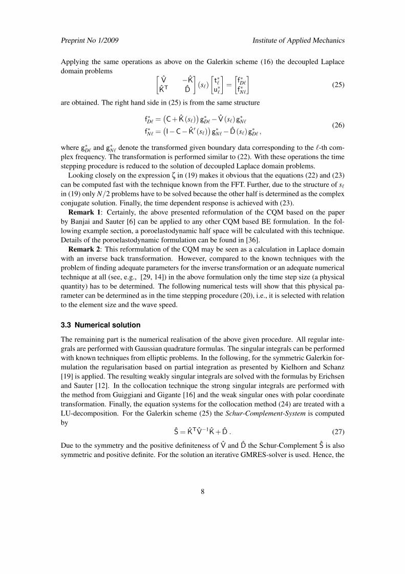
Applying the same operations as above on the Galerkin scheme (16) the decoupled Laplacedomain problems [

V −K

KT D

](s`)

[t∗`u∗`

]=[f∗D`

f∗N`

](25)

are obtained. The right hand side in (25) is from the same structure

f∗D` =(C+ K(s`)

)g∗D`− V (s`)g∗N`

f∗N` =(I−C− K′ (s`)

)g∗N`− D(s`)g∗D` ,

(26)

where g∗D` and g∗N` denote the transformed given boundary data corresponding to the `-th com-plex frequency. The transformation is performed similar to (22). With these operations the timestepping procedure is reduced to the solution of decoupled Laplace domain problems.

Looking closely on the expression ζ in (19) makes it obvious that the equations (22) and (23)can be computed fast with the technique known from the FFT. Further, due to the structure of s`

in (19) only N/2 problems have to be solved because the other half is determined as the complexconjugate solution. Finally, the time dependent response is achieved with (23).

Remark 1: Certainly, the above presented reformulation of the CQM based on the paperby Banjai and Sauter [6] can be applied to any other CQM based BE formulation. In the fol-lowing example section, a poroelastodynamic half space will be calculated with this technique.Details of the poroelastodynamic formulation can be found in [36].

Remark 2: This reformulation of the CQM may be seen as a calculation in Laplace domainwith an inverse back transformation. However, compared to the known techniques with theproblem of finding adequate parameters for the inverse transformation or an adequate numericaltechnique at all (see, e.g., [29, 14]) in the above formulation only the time step size (a physicalquantity) has to be determined. The following numerical tests will show that this physical pa-rameter can be determined as in the time stepping procedure (20), i.e., it is selected with relationto the element size and the wave speed.

3.3 Numerical solution

The remaining part is the numerical realisation of the above given procedure. All regular inte-grals are performed with Gaussian quadrature formulas. The singular integrals can be performedwith known techniques from elliptic problems. In the following, for the symmetric Galerkin for-mulation the regularisation based on partial integration as presented by Kielhorn and Schanz[19] is applied. The resulting weakly singular integrals are solved with the formulas by Erichsenand Sauter [12]. In the collocation technique the strong singular integrals are performed withthe method from Guiggiani and Gigante [16] and the weak singular ones with polar coordinatetransformation. Finally, the equation systems for the collocation method (24) are treated with aLU-decomposition. For the Galerkin scheme (25) the Schur-Complement-System is computedby

S = KTV−1K+ D . (27)

Due to the symmetry and the positive definiteness of V and D the Schur-Complement S is alsosymmetric and positive definite. For the solution an iterative GMRES-solver is used. Hence, the

8


` = 3m

x

y

ty =−1 N/m2H(t)

(a) Geometry and load (b) Mesh of the 3m×1m×1m column

Figure 1: Geometry, loading, and the mesh of the column

displacement field u∗` and the tractions t∗` can be found by solving

Su∗` = f∗N`− KTV−1f∗D` (28)

andt∗` = V−1 (f∗D` + Ku∗`

)(29)

for every complex frequency s`, ` = 0, . . . ,N/2.

4 Numerical examples

In this section, the numerical behavior of this reformulated CQM in the application on an elas-todynamic column is studied. Further, results for wave propagation phenomena in a poroelastichalf space are presented. For all computations a Backward Difference Formula of second order(BDF2) as multistep method is used. The parameter R can be adjusted as in the original formu-lation to RN =

√ε with 10−10 < ε < 10−3 which may vary between different physical problem

types and between 2-d and 3-d. However, it is independent of the geometry and boundary con-ditions.

4.1 Elastic column

A one dimensional (1-d) column of length 3m as sketched in Fig. 1(a) is considered. It isassumed that the side walls and the bottom are rigid and frictionless. Hence, the displacementsnormal to the surface are blocked and the column is otherwise free to slide only parallel tothe wall. At the top, the stress vector ty = −1 N/m2H(t) is given. Due to these restrictions,the 3-d continuum is reduced to a 1-d column with the only degree of freedom in y-direction.This 1-d column has been solved analytically in [15] and its result is compared to the boundaryelement solution for a 3-d rod (3m× 1m× 1m). The used BE formulation is the symmetricGalerkin scheme sketched before, where the traction field is approximated on linear triangles

9


Table 1: Material data for the elastic column and the poroelastic half spaceE ν ρ φ R ρ f α κ

N/m2 - kg/m3 - N/m2 kg/m3 - m4/Ns

elastic column

steel 2.11 ·1011 0 7850

poroelastic half space

soil 2.544 ·108 0.298 1884 0.48 1.2 ·109 1000 0.981 3.55 ·10−9

with constant shape functions and the displacement field with linear ones. Material data usedare those of steel modified with Poisson’s ratio set to zero (see Tab. 1).

The meshes used in the following are four different ones which are basically a refinement orcoarsening of that shown in Fig. 1(b). They will be denoted

• mesh 1: uniform with 112 elements on 58 nodes

• mesh 2: uniform with 448 elements on 226 nodes

• mesh 3: uniform with 700 elements on 352 nodes as displayed in Fig. 1(b)

• mesh 4: uniform with 2800 elements on 1402 nodes.

In Fig. 2, the displacement results versus time at the free end are plotted for the meshes 1,2,and 3. The time step size for all three calculations are adjusted to β = 0.3. This dimensionlessvalue used for the comparison is β = c1∆t/re, with the characteristic length of the elements re.Here, the cathethus of the triangles is used. The differences for the displacements in Fig. 2are not too large. In the second half of the figure, the tractions at the bottom of the columnshow differences. The coarsest mesh 1 yields not satisfactory results for larger times. Theovershooting following the jumps in the solution are unavoidable but a refined mesh reduces theduration of this disturbance. It is exactly the same behavior as in the ’old’ CQM based BEMas presented, e.g., in [19]. That is why no comparison between the old formulation and thereformulated version is given. They can not be distinguished in a plot.

In Fig. 3, the displacement at the top and the traction at the bottom are plotted versus time fordifferent time step sizes. These are expressed with β to have a better comparison. The results arecomputed with mesh 2. The instability for the smallest value β = 0.1 is clearly observed in thetraction solution. The other extreme value, β = 0.7, shows some numerical damping and not thebest results for the traction. All other results are acceptable, where as in the original formulationa value β = 0.2 yields the best results. Hence, also the sensitivity on the choice of the time stepsize is the same as in the original formulation. A time step size in the range 0.1 < β < 0.5 maybe recommended.

It must be remarked that here the main advantage of the presented formulation compared tousual computations in Laplace or Fourier domain can be observed. The parameter responsiblefor the quality of the results is the time step size and not any sophisticated parameter of the

10


0 0.002 0.004 0.006time t [s]

0

5e-12

1e-11

1.5e-11

2e-11

2.5e-11

3e-11

disp

lace

men

t u2 [m

]

analyticmesh 1mesh 2mesh 3

(a) Displacement at the top

0 0.002 0.004 0.006time t [s]

-2

-1.5

-1

-0.5

0

tract

ion

t 2 [N/m

2 ] analyticmesh 1mesh 2mesh 3

(b) Traction at the bottom

Figure 2: Displacement and traction versus time for different meshes compared with the analyt-ical solution

11


0 0.002 0.004 0.006time t [s]

0

5e-12

1e-11

1.5e-11

2e-11

2.5e-11

3e-11

disp

lace

men

t u2 [m

]

analyticβ = 0.1β = 0.2β = 0.5β = 0.7

(a) Displacement at the top

0 0.002 0.004 0.006time t [s]

-2

-1.5

-1

-0.5

0

tract

ion

t 2 [N/m

2 ] analyticβ = 0.1β = 0.2β = 0.5β = 0.7

(b) Traction at the bottom

Figure 3: Displacement and traction versus time for different time step sizes, i.e., β values, com-pared with the analytical solution

12


0 0.002 0.004 0.006time t [s]

-2

-1.5

-1

-0.5

0

tract

ion

t 2 [N/m

2 ]

ε = 10−2

ε = 10−3

ε = 10−8

Figure 4: Traction versus time for different precisions ε of the iterative solver

various numerical inverse transformation algorithms. This value is oriented on the physics ofthe problem, i.e., it must be adjusted to the wave speed in relation to the mesh size.

The next parametric study concerns the solution of the equation system. For larger problemsiterative solvers may be used. Hence, the question arise what is the influence of the solverprecision on the time dependent results. Here, a GMRES is used. In Fig. 4, the traction solutionsfor mesh 4 are plotted calculated with different precisions of the GMRES. The displacementsolutions are not displayed because no differences would be visible. In the traction solution,only for the coarse value of ε = 10−2 negative effects for large times may be observed. It maybe concluded that the solver precision is not so important. But, it must be remarked that thesolver works in Laplace domain and, hence, eigenfrequencies even if they are damped maycause problems. Further, it is recommended to think on proper preconditioners. Last, it shouldbe mentioned that this ε has nothing to do with the ε to determine R as discussed at the beginingof this section.

4.2 Poroelastic half space

The second example is a poroelastic half space modelled with Biot’s theory. The collocation BEformulation proposed in [35] with the new formulation of the CQM is applied. To be able tosolve the equation system dimensionless variables are introduced as suggested in [39]. Detailsof the poroelastic BE formulation based on the reformulation of the CQM and numerical studieson the sensitivity with respect to the time step size can be found in [36]. These tests confirm theobservation in the paragraph above, the new formulation behaves like the old one.

The following results are obtained with linear shape functions for all unknowns, i.e., the solid

13


A

z

P

15 m

y

z

x −1000

t

t

Figure 5: Poroelastic half space: Mesh and the time dependence of the load

displacements, the pore pressure, the tractions, and the flux. The geometry is approximatedby linear triangles as sketched in Fig. 5. The half space is loaded in area A by a total stressvector tz =−1000 N/m2H(t) kept constant from t = 0s on. The material data are those of a watersaturated soil taken from literature [20] and listed in Tab. 1. There, φ,R,ρ f ,α, and κ denotethe porosity, Biot’s constant, density of the fluid, Biot’s stress coefficient, and the permeability,respectively.

In Fig. 6, the vertical solid displacement uz is plotted versus time for the point P in 15mdistance to the load. The poroelastic result is compared to two elastodynamic solutions denotedby ’drained’ and ’undrained’. This means the shear modulus is the same as in the poroelasticcase but in the drained case the same Poisson’s ratio is used whereas in the undrained case theundrained Poisson’s ratio is inserted. Additionally, a calculation with the ’old’ CQM based BEformulation is presented, lying over the ’new’ CQM based formulation.

The arrival time of the compression wave t ≈ 0.014s and the Rayleigh pole are clearly ob-served. Further, as expected, the poroelastic solution is between the two extreme elastodynamiccases, whereas in the early time it follows the undrained behavior and later (in the second halfof the picture) it approaches the drained solution. The solution denoted ’long time’ is obtainedwith a very large time step size to reach such long observation times. That is the reason why thissolution in the short time range does not resolve the arrival of the waves correctly.

5 Conclusion

A reformulated version of the Convolution Quadrature Method (CQM) has been applied to theelastodynamic boundary integral equation in time domain. Both, a symmetric Galerkin methodand a collocation method has been presented. Clearly, this reformulation of the CQM can be

14


0 0.03 0.06 0.09 0.12time t [s]

-1e-07

-5e-08

0

5e-08di

spla

cem

ent u

z [m]

drained∆t = 0.0007 sundrainedlong timeold CQM

10 20 30 40 50

Figure 6: Vertical displacement at point P: Short and long time behavior

applied to any other application in time domain BE formulations. Here, additionally to theelastodynamic example a poroelastodynamic example has been shown. Overall, the presentedmethodology reduces the storage requirement to the size of one complex valued system matrixand shows the same sensitivity on the time step size as the older formulation presented by Schanz[35]. The price to be payed for this reduction in storage is that in each step the system ofequations has to be solved. But, for future work, this reformulated CQM allows the applicationof fast BE techniques which are mostly known for elliptic problems and not for hyperbolic ones.

In some sense this reformulation is similar to classical formulations in Laplace or Fourierdomain with numerical inverse transformations. It shares the disadvantage that the time historyof the given boundary data has to be known in advance. However, contrary to the usual inversetransformation algorithms, here, the only parameter to be adjusted is the time step size. Thisparameter is determined with respect to the wave speed and the spatial mesh size. Hence, itdepends only on physical values and not on some sophisticated parameters as in usual numericalinverse transformation formulas.

Acknowledgement The author gratefully acknowledges the financial support by the AustrianScience Fund (FWF) under grant P18481-N13. The fruitful and helpful discussion with L.Banjai and S. Sauter during the author’s stay at the University of Zürich is as well gratefullyacknowledged.

15


References

[1] A. I. Abreu, J. A. M. Carrer, and W. J. Mansur. Scalar wave propagation in 2D: a BEMformulation based on the operational quadrature method. Eng. Anal. Bound. Elem., 27:101–105, 2003.

[2] A. I. Abreu, W. J. Mansur, and J. A. M. Carrer. Initial conditions contribution in a BEMformulation based on the convolution quadrature method. Int. J. Numer. Methods. Engrg.,67:417–434, 2006.

[3] S. Ahmad and G. D. Manolis. Dynamic analysis of 3-D structures by a transformed bound-ary element method. Comput. Mech., 2:185–196, 1987.

[4] H. Antes. A boundary element procedure for transient wave propagations in two-dimensional isotropic elastic media. Finite Elements in Analysis and Design, 1:313–322,1985.

[5] H. Antes and M. Jäger. On stability and efficiency of 3d acoustic BE procedures for movingnoise sources. In S.N. Atluri, G. Yagawa, and T.A. Cruse, editors, Computational Mechan-ics, Theory and Applications, volume 2, pages 3056–3061, Heidelberg, 1995. Springer-Verlag.

[6] L. Banjai and S. Sauter. Rapid solution of the wave equation in unbounded domains. SIAMJ. Numer. Anal., 47(1):227–249, 2009.

[7] D. E. Beskos. Boundary element methods in dynamic analysis. AMR, 40(1):1–23, 1987.

[8] D. E. Beskos. Boundary element methods in dynamic analysis: Part II (1986-1996). AMR,50(3):149–197, 1997.

[9] T. A. Cruse and F. J. Rizzo. A direct formulation and numerical solution of the generaltransient elastodynamic problem, I. Aust. J. Math. Anal. Appl., 22(1):244–259, 1968.

[10] J. Domínguez. Boundary Elements in Dynamics. Computational Mechanics Publication,Southampton, 1993.

[11] J. Domínguez. Dynamic stiffness of rectangular foundations. Report no. R78-20, Depart-ment of Civil Engineering, MIT, Cambridge MA, 1978.

[12] S. Erichsen and S. A. Sauter. Efficient automatic quadrature in 3-d Galerkin BEM. Comput.Methods Appl. Mech. Engrg., 157(3–4):215–224, 1998.

[13] F. García-Sánchez, Ch. Zhang, and A. Sáez. 2-d transient dynamic analysis of crackedpiezoelectric solids by a time-domain BEM. Comput. Methods Appl. Mech. Engrg., 197(33-40):3108–3121, 2008.

[14] L. Gaul and M. Schanz. A comparative study of three boundary element approaches tocalculate the transient response of viscoelastic solids with unbounded domains. Comput.Methods Appl. Mech. Engrg., 179(1-2):111–123, 1999.

16


[15] K. F. Graff. Wave Motion in Elastic Solids. Oxford University Press, 1975.

[16] M. Guiggiani and A. Gigante. A general algorithm for multidimensional cauchy principalvalue integrals in the boundary element method. J. of Appl. Mech., 57:906–915, 1990.

[17] W. Hackbusch, W. Kress, and S. A. Sauter. Sparse convolution quadrature for time domainboundary integral formulations of the wave equation by cutoff and panel-clustering. InM. Schanz and O. Steinbach, editors, Boundary Element Analysis: Mathematical Aspectsand Applications, volume 29 of Lecture Notes in Applied and Computational Mechanics,pages 113–134. Springer-Verlag, Berlin Heidelberg, 2007.

[18] E. Kausel. Fundamental Solutions in Elastodynamics. Cambridge University Press, 2006.

[19] L. Kielhorn and M. Schanz. Convolution quadrature method based symmetric Galerkinboundary element method for 3-d elastodynamics. Int. J. Numer. Methods. Engrg., 76(11):1724–1746, 2008.

[20] Y. K. Kim and H. B. Kingsbury. Dynamic characterization of poroelastic materials. Exp.Mech., 19(7):252–258, 1979.

[21] C. Lubich. Convolution quadrature and discretized operational calculus. I. Numer. Math.,52(2):129–145, 1988.

[22] C. Lubich. Convolution quadrature and discretized operational calculus. II. Numer. Math.,52(4):413–425, 1988.

[23] Ch. Lubich. Convolution quadrature revisited. BIT Num. Math., 44(3):503–514, 2004.

[24] Ch. Lubich. On the multistep time discretization of linear initial-boundary value problemsand their boundary integral equations. Numer. Math., 67:365–389, 1994.

[25] Ch. Lubich and R. Schneider. Time discretization of parabolic boundary integral equations.Numer. Math., 63:455–481, 1992.

[26] G. D. Manolis. A comparative study on three boundary element method approaches toproblems in elastodynamics. Int. J. Numer. Methods. Engrg., 19:73–91, 1983.

[27] W. J. Mansur. A Time-Stepping Technique to Solve Wave Propagation Problems Using theBoundary Element Method. Phd thesis, University of Southampton, 1983.

[28] W. J. Mansur, J. A. M. Carrer, and E. F. N. Siqueira. Time discontinuous linear tractionapproximation in time-domain BEM scalar wave propagation. Int. J. Numer. Methods.Engrg., 42(4):667–683, 1998.

[29] G. V. Narayanan and D. E. Beskos. Numerical operational methods for time-dependentlinear problems. Int. J. Numer. Methods. Engrg., 18:1829–1854, 1982.

[30] D. Nardini and C. A. Brebbia. A new approach to free vibration analysis using boundaryelements. In C. A. Brebbia, editor, Boundary Element Methods, pages 312–326. Springer-Verlag, Berlin, 1982.

17


[31] P. W. Partridge, C. A. Brebbia, and L. C. Wrobel. The Dual Reciprocity Boundary ElementMethod. Computational Mechanics Publication, Southampton, 1992.

[32] A. Peirce and E. Siebrits. Stability analysis and design of time-stepping schemes for gen-eral elastodynamic boundary element models. Int. J. Numer. Methods. Engrg., 40(2):319–342, 1997.

[33] D. C. Rizos and D. L. Karabalis. An advanced direct time domain BEM formulation forgeneral 3-D elastodynamic problems. Comput. Mech., 15:249–269, 1994.

[34] M. Schanz. Application of 3-d Boundary Element formulation to wave propagation inporoelastic solids. Eng. Anal. Bound. Elem., 25(4-5):363–376, 2001.

[35] M. Schanz. Wave Propagation in Viscoelastic and Poroelastic Continua: A BoundaryElement Approach, volume 2 of Lecture Notes in Applied Mechanics. Springer-Verlag,Berlin, Heidelberg, New York, 2001.

[36] M. Schanz. Storage reduced poroelastodynamic boundary element formulation in timedomain. In H. I. Ling, A. Smyth, and R. Betti, editors, Poromechanics IV, pages 902–907,Lancaster, 2009. DEStech Publications, Inc.

[37] M. Schanz and H. Antes. Application of ‘operational quadrature methods’ in time domainboundary element methods. Meccanica, 32(3):179–186, 1997.

[38] M. Schanz and H. Antes. A new visco- and elastodynamic time domain boundary elementformulation. Comput. Mech., 20(5):452–459, 1997.

[39] M. Schanz and L. Kielhorn. Dimensionless variables in a poroelastodynamic time domainboundary element formulation. Building Research Journal, 53(2-3):175–189, 2005.

[40] O. Steinbach. Numerical Approximation Methods for Elliptic Boundary Value Problems,volume 54 of Texts in Applied Mathematics. Springer, 2008.

[41] L. T. Wheeler and E. Sternberg. Some theorems in classical elastodynamics. Arch. RationalMech. Anal., 31:51–90, 1968.

[42] G. Yu, W. J. Mansur, J. A. M. Carrer, and L. Gong. Time weighting in time domain BEM.Eng. Anal. Bound. Elem., 22(3):175–181, 1998.

[43] G. Yu, W. J. Mansur, J. A. M. Carrer, and L. Gong. Stability of Galerkin and Collocationtime domain boundary element methods as applied to the scalar wave equation. Comput.& Structures, 74(4):495–506, 2000.

[44] Ch. Zhang. Transient elastodynamic antiplane crack analysis in anisotropic solids. Inter-nat. J. Solids Structures, 37(42):6107–6130, 2000.

18

preprint series institute of applied mechanics graz university of technology · 2015-10-29 ·...

Documents