preschool, day care, and after school care: who’s … · preschool, day care, and after school...
TRANSCRIPT

1
Preschool, Day Care, and After School Care: Who’s Minding the Kids?
David Blau
(UNC-Chapel Hill)
Janet Currie
(UCLA and NBER)
June, 2003
Abstract The majority of children in the U.S. and many other high-income nations are now cared for many hours per week by people who are neither their parents nor their school teachers. The role of such pre-school and out of school care is potentially two-fold: First, child care makes it feasible for both parents or the only parent in a single-parent family to be employed. Second, early intervention programs and after school programs aim to enhance child development, particularly among disadvantaged children. Corresponding to this distinction, there are two branches of literature to be summarized in this chapter. The first focuses on the market for child care and analyzes factors affecting the supply, demand and quality of care. The second focuses on child outcomes, and asks whether certain types of programs can ameliorate the effects of early disadvantage. The primary goal of this review is to bring the two literatures together in order to suggest ways that both may be enhanced. Accordingly, we provide an overview of the number of children being cared for in different sorts of arrangements; describe theory and evidence about the nature of the private child care market; and discuss theory and evidence about government intervention in the market for child care. Our summary suggests that additional research is necessary to highlight the ways that government programs and market provided child care interact with each other. Keywords: Preschool, Child care, daycare, Early intervention, Head Start, Afterschool programs, Child care subsidies. JEL codes: I21, I28, I38
We would like to thank Ilya Berger, Stephanie Riegg and Jwahong Min for excellent research assistance, and Jeanne Brooks-Gunn and participants in the Handbook on the Economics of Education Conference of March 2003 for helpful comments.

2
Outline:
1. Introduction
2. Who’s Minding the Kids?
3. The Market For Child Care
A: Demand for Child Care 1. Theory
2. Evidence B: Supply of Child Care
1. The Quantity of Child Care Supplied 2. The Supply of Quality in Child Care Centers
C: The Effect of Child Care Quality on Children 4. Governmental Intervention in the Child Care Market
A: Rationale B: Subsidies C: Regulations
5. Publicly Provided Child Care A: Model Early Intervention Programs
B: Head Start C: Early Head Start D: State Programs E: Programs for School Aged Children 6. Unanswered Questions List of Tables and Figures: Table 1: Characteristics of Households with Children 0-4 by Type of Child Care Arrangement Table 2: Characteristics of Households with Children 5-14 by Type of Child Care Arrangement

3
Table 3: Trends in Child Care Arrangements and Expenditures Table 4: Distribution of Children Ages 5-14 by Use of Self Care and Mother’s Employment Status, 1999 Table 5: Studies of the Effects of the Price of Child Care on Employment of Mothers Table 6: Characteristics of Day Care Centers and Regulated Family Day Care Homes, 1990 Table 7: The Distribution of Child Care Quality in Day Care Centers Table 8: Studies of the Effects of Child Care Inputs on Quality and on Child Outcomes Table 9: Summary of the History, Goals, and Provisions of Major Federal Child Care Programs Table 10: Characteristics of State Child Care and Development Fund Plans Table 11: Federal and State Expenditures and Children Served by Major Child Care Subsidy Programs Table 12: Incidence of Child Care Subsidy Receipt and Characteristics of Recipients, 1999 Table 13: Studies of the Effect of Child Care Subsidies on Employment Table 14: Selected State Child Care Regulations Table 15: Studies of the Effects of Regulations on Child Care Use Table 16: Model Early Childhood Programs with Randomized Designs Table 17: Large Scale Public Early Childhood Programs Table 18: State Spending on Pre-Kindergarten Initiatives Table 19: Studies of the Effects of Self-Care on Child Outcomes Table 20: Studies of the Effects of After school Programs on Child Outcomes Table 21: Studies of the Effects of Positive Youth Development Programs on Child Outcomes Figure 1: Effects of Non-Linear Subsidies on Hours of Work

1
1. Introduction:
For good or ill, the majority of children in the U.S. and many other high-income nations are now
cared for many hours per week by adults other than their parents and school teachers. The role of such
pre-school and out of school care is potentially two-fold: First, child care can make it feasible for both
parents or the only parent in a single-parent family to be employed. This role has become increasingly
important in an era of welfare reform, in which able bodied mothers are expected to work regardless of
the age of their children. Second, early intervention programs and after school programs can enhance
child development, particularly among disadvantaged children. Consistent with this distinction, child
care is typically provided by the private market, while early intervention programs are generally publicly
provided.
Corresponding to this distinction, there are two branches of literature to be summarized in this
chapter. The first focuses on the market for child care and analyzes factors affecting the supply, demand
and quality of care. The second focuses on child outcomes, and asks whether certain types of programs
can ameliorate the effects of early disadvantage. However, child care and early intervention are
intrinsically linked: The quality of child care is likely to affect child development, and programs such as
Head Start which seek to enhance child development also provide child care. Moreover, National
Research Council and Institute of medicine (2003) estimates that in the U.S., one third of the costs of
child care for children under age six is paid for by government subsidies. The primary goal of this
review is to bring the two literatures together in order to suggest ways that both may be enhanced. Our
summary suggests that additional research is necessary to highlight the ways that government programs
and market provided child care interact with each other.
Section 2 provides an overview of the number of children being cared for in different sorts of
arrangements. Section 3 describes theory and evidence about the nature of the child care market. Section
4 discusses theory and evidence on government intervention in the market for child care, while section 5
discusses direct government provision of services. Section 6 offers conclusions and suggestions for
further research. This review follows the literature in focusing on the United States . As Waldfogel
(2001) emphasizes, there are dramatic differences between OECD countries in the extent to which child

2
care policies are publicly supported. Exploring the effects of child care policy in other countries would be
an interesting topic for future research.
2. Who is Minding the Kids?
The dramatic increase in female labor force participation is one of the most important
developments in the postwar U.S. economy. This increase has been greatest among married women with
children. For example, in 1950 11.9% of married women with children under six were in the labor force,
compared to 62.8% in 2000. Never married, separated, and divorced mothers also increased their labor
force participation dramatically, with the most rapid growth in the last three decades. In 2000, 65.3% of
single women with children under 6 were in the work force (U.S. Bureau of Labor Statistics, 2001), and
the National Institutes for Child Health and Development (NICHD) Early Child Care Study found that
most infants were placed in some sort of non-maternal care by four months of age (NICHD Early
Childcare Research Network, 1997). In a recent press release calling attention to the “record”
participation rates of women with young children, the Census bureau noted that “The large increase in
labor force participation rates by mothers since 1976 is an important reason why child-care issues have
been so visible in recent years” (U.S. Census Bureau, October 24, 2000.)
However, child care is also increasingly utilized by families with stay-at-home parents. Tables 1
and 2 present tabulations of the type of child care used by children aged 0-4 and 5-14 in 1999,
disaggregated by the mother’s employment status. Table 1 shows that almost a third of 0 to 4 year old
children with mothers who are not employed are in non-parental child care, compared to three quarters of
children of employed mothers (lower panel, first row). The former group spends an average of 16 to 20
hours per week in the primary mode of non-parental care, and 20-27 percent also spend a further 7 to 11
hours in a secondary mode of non-parental care. This is a substantial amount of time, although much less
than the 32 to 35 hours per week that children of employed mothers spend in their primary non-parental
care arrangement. It is striking that a large fraction of care is not paid for, particularly in families in
which the mother is not employed. For the latter group, about half of non-relative and center care is
unpaid, compared to 10-20 percent for employed mothers. Families with a non-employed mother are also

3
more likely to receive government assistance in paying for child care.
Table 1 also shows that there are distinct demographic patterns in the use of child care modes.
Relative to white non-Hispanic mothers, black mothers are more likely to use care from relatives, or child
care centers, and less likely to use non-relative care. Hispanic mothers are most likely to use relative
care, and least likely to use centers, a pattern that has been noted previously (c.f. Fuller et al. 1996;
Hofferth et al., 1991). The use of center-based care is distinctly U-shaped with respect to income, with
both poor and rich families more likely to use such care than middle income households, and families on
public assistance being more likely to use such care than other families. There are also pronounced
regional differences, though urban and rural families tend to have fairly similar patterns of mode choice.
For example, mothers in the South are more likely to use center-based care than those in the rest of the
country.i Not surprisingly, younger children are more likely to be cared for by parents than older
children, as are children of married mothers.
Table 2 indicates that 63% of school age children of employed mothers regularly spend time in
some form of non-school, non-parental care, compared to 31 percent of children of non-employed
mothers. Children of employed mothers spend an average of 22 to 30 hours a week in such
arrangements. Considering that most children spend about 30 hours a week in school, it is evident that
what they do during this non-school care time is likely to be important to their development. In contrast
to younger children, school-age children spend relatively little time in non-relative care, and greater
amounts of time in organized activities. Two thirds to three quarters of these activities involve a
monetary payment, so it is not surprising that white children are more likely to be involved than black
and especially Hispanic children, or that poorer children are less likely to have organized activities than
richer ones.
The vast increase in maternal employment has generated a large literature on the effects of
maternal employment on child outcomes (c.f. Baum, 2002; Belsky and Eggebeen, 1991; Blau and
Grossberg, 1992; Desai, Chase-Lansdale and Michael, 1989; Greenstein, 1993; Han, Waldfogel, and iBlau (2001) notes that mothers in the South are substantially more likely to be employed full time than are mothers in other regions.

4
Brooks-Gunn, 2001; Neidell, 2000; Parcel and Menaghan, 1990, 1994; Ruhm, 2000; Waldfogel et al.,
2002). This literature has produced little conclusive evidence of a negative effect of maternal
employment on children. Although OLS estimates often shownegative effects of employment in the first
year, these effects are not generally robust to attempts to deal with the endogeneity of employment. The
small or negligible effects may be because the increased income earned by employed mothers offsets the
effect of reduced time spent with their children. However, time use studies indicate that except for very
young children, maternal employment has only modest effects on the amount of time mothers spend with
their children, and tends to increase the amount of time that fathers spend with their children in two-
parent households. Mothers apparently reduce both leisure time and housework in order to maintain their
time inputs into child raising (National Research Council and Institute of Medicine, 2003).
The most consistent evidence of negative effects of maternal employment comes from families in
which some or all of the following are true: the mother returns to work when the child is less than one
year old; young children spend very long hours in care; the mother’s employment does not raise family
income (as in some households where families have been forced off welfare); there is a single parent with
few family members to draw on so that time spent in employment cannot be compensated by drawing on
the time of other family members either for child care or for housework; and/or the work itself is very
stressful and reduces the resources the mother brings to parenting. Some studies of shift-work, for
example, suggest that it may have this effect. Adolescents may also suffer more negative effects of
maternal employment than younger children, particularly if they are left unsupervised. (National
Research Council and Institute of Medicine, 2003).
Table 3 focuses on trends in the use of child care by employed mothers. Perhaps surprisingly, the
percentage of preschool children in organized facilities shows no clear trend between 1985 and 1999,
although the number of children reporting relative care as their primary arrangement increases.ii The
iiA CPS supplement in June 1977 collected data on child care used by children of employed mothers. There were 4.37 million children under age 5 at that time, and their distribution of modes of care was father:14.4%; relative (including grandparent): 30.9%; babysitter in the child’s home: 7.0%; family day care home: 22.4%; day care center/preschool: 13.0%; mother while working: 11.4% (Casper, 1997). Thus, the major increase in use of centers occurred between 1977 and 1985.

5
fraction of families who report paying for child care increased over time, from 33.7% in 1985 to 43% in
1999, although the average amount paid fell in real terms. Since the percentage of income paid for child
care increased over the same period, Table 3 suggests that more low-income families are paying for child
care.
Table 4 addresses the issue of so-called “latch-key” children, who spend some part of the day
without any adult supervision. In 1999, 10.5% of children age 5 to 14 of employed mothers were in
unsupervised self-care for part of the day, compared to 3.2% of children of non-employed mothers.
Most of these children were in relative care as their primary child care arrangement. This suggests that
employed mothers who rely on care from relatives are often unable to schedule activities so that all of the
child's time can be supervised. As one might expect, the fraction of children who are unsupervised rises
sharply with age: among 9 year old children of employed mothers, 8.1% are sometimes unsupervised
(5.2/(5.2+59.1))compared to 18.1% among 11 year olds (11.5/(11.5+51.9)) and 44.9% of 14 year olds
(32.3/(32.3+39.7)). The probability of being unsupervised is higher for single parents, and also rises with
income. It is also lower for Hispanics and Blacks than for Whites.
There is evidence that unsupervised children are at increased risk of truancy, poor grades, and
risk-taking behaviors such as substance abuse (Dwyer et al., 1990). Juvenile crime rates triple in the after
school hours between 3 and 6 in the afternoon when children are most likely to be left unattended, and
children are most likely to be victims of violent crimes committed by non-family members in these hours
(Fox and Neuman, 1997; U.S. Office of Juvenile Justice and Delinquency Prevention, 1996). These facts
suggest that lack of supervision is a serious problem, at least for some children—an issue we revisit in
Section 6.
In summary, large numbers of children spend many hours each week in some form of non-
parental, non-school child care. While children of employed mothers are most likely to be in child care, a
significant share of children with non-employed mothers are also in child care. Many children spend time
in more than one mode of non-parental care, and routinely spend time unsupervised, suggesting that it is
difficult for some parents to patch together enough child care to completely cover the necessary hours.

6
3. The Market for Child Care
A. Demand for Child Care
1. Theory
A simple one-person static labor supply model augmented with assumptions about child care
provides a useful starting point for analyzing demand for child care . The mother is the agent in the
model, making decisions about care for her children. Suppose that child care is homogeneous in quality
and commands a market price of p dollars per hour of care per child, taken as given by the mother.iii
There is no informal unpaid care available and the mother cannot care for her children while she works,
so paid child care is required for every hour the mother works. By assumption, the mother cares for her
children during all hours in which she is not working. There are no fixed costs of work, and the wage rate
w is the same for each hour of work. For simplicity, suppose there is only one child who needs care. The
mother’s budget constraint is c = y + (w-p)h, where c is consumption expenditure other than child care, y
is nonwage income, and h is hours of work. The time constraint is h + l = 1, where l is hours of leisure,
and the utility function is u(c, l). The monetary cost of child care reduces the net wage rate (w-p). A
higher price of child care increases the likelihood that the net market wage is below the reservation wage,
thereby reducing the likelihood of employment.
Some families have access to care by a relative, including the father or another family member, at
no monetary cost. But not all families with access to such care use it, because it has an opportunity cost:
the relative sacrifices leisure or earnings in order to provide care. The quality of such care compared to
the quality of market care is also likely to influence the use of informal care, but consideration of quality
is taken up below and ignored here. If the mother pools income with the relative or has preferences over
the relative’s leisure hours, then the mother will behave as if unpaid child care has an opportunity cost. To
illustrate in the simplest possible setting, take as given that the relative who is the potential unpaid child
care provider is not employed.iv Let H represent hours of paid child care purchased in the market and U iiiHomogeneous quality means that we can ignore the effect of child care on child outcomes for now. This assumption will be relaxed below.
ivSee Blau and Robins (1988) for a model in which the relative’s employment status is a choice variable. This extension does not change the qualitative implications of the analysis.

7
hours of unpaid child care. Maintaining the assumption that the mother is the care giver during all hours
in which she is not employed, we have h = H + U, and h ≥ H, U ≥ 0. The budget constraint is c = y + wh -
pH. The utility function is u(c, l, lr), where lr is leisure hours of the relative. The time constraints are l + h
= 1 for the mother, and lr + U = 1 for the relative. If U and H are both positive, then the shadow price of
an hour of relative care is the marginal utility of the relative’s leisure. In this case relative care is used for
the number of hours U* for which the marginal rate of substitution between consumption and leisure of
the relative equals the market price of care: ulr/uc=p; and paid care is used for the remaining H* = h - U*
hours for which child care is required.
In order to examine work incentives in this model, classify outcomes as follows:
Outcome Mother Employed Unpaid Care Used Paid Care Used 1 no no no 2 yes yes no 3 yes yes yes 4 yes no yes
A higher price of child care increases the cost of using paid care, but does not affect the cost of unpaid
relative care, because no money changes hands for such care. A higher price therefore decreases the
probability of choosing outcomes 3 and 4, and increases the probability of choosing outcomes 1 and 2. In
addition to providing a work disincentive for the mother (outcome 1 is more likely) a higher price also
provides an incentive to use unpaid care conditional on working (outcome 2 is more likely).
If the quality of paid child care is variable and if the quality of care affects child outcomes, then
the mother will be concerned about the quality of care she purchases. The simplest case to consider is uni-
dimensional quality: quality is a single “thing.” The price of an hour of child care is p = α + βq, where q
is the quality of care and α and β are parameters determined in the market. This hedonic price function is
determined by the market supply of and demand for quality (a linear price function is not essential to the
argument). The mother cares about the quality of child care because it affects her child’s development
outcome, d. Let the child development production function be d = d(lqm, hq), where qm is the quality of
the care provided by the mother. The effect of purchased child care on development depends on its
quantity (h) and quality (q). For simplicity, no distinction is made between the mother’s leisure and her

8
time input to child development, and assume also for simplicity that no unpaid care is available. Relaxing
these assumptions does not change the main implications of this model. The utility function is u(c, l, d)
and the budget constraint is c = y + (w – [α + βq])h.
Blau ( 2003b) demonstrates the following results in this model. A higher price of child care
resulting from an increase in either α or β decreases the incentive to be employed. An increase in α has a
bigger negative effect on employment than an equivalent increase in β. So, if the goal of a subsidy
program is to facilitate employment, this is best accomplished by an “α-subsidy” unconditional on
quality. In a quality-quantity model such as this one, the substitution effect of a change in price on the
level of quality demanded is ambiguous, and this holds for changes in both α and β. But it can be shown
that (1) if the substitution effects ∂ q/ ∂ α| u and ∂ q/ ∂ β| u are both negative, then ∂ q/ ∂ β| u is larger in
absolute value than ∂ q/ ∂ α| u ; and (2) if ∂ q/ ∂ α| u >0 then either ∂ q/ ∂ β| u is positive but smaller than
∂ q/ ∂ α| u , or ∂ q/ ∂ β| u <0. Thus an increase in β has a bigger negative effect or a smaller positive effect
on the level of quality demanded than an increase in α. So if the goal of a subsidy is to improve the
quality of child care, a “β-subsidy” that provides a more generous subsidy for higher-quality care is more
effective than an α-subsidy. There is a clear tradeoff in subsidy policy between the goals of increasing
employment and improving the quality of child care.
2. Evidence
Table 5 summarizes results from 20 studies that estimated the effect of the price of purchased
child care on the employment of mothers.v Estimated price elasticities reported in the studies range from
.06 to -3.60. The studies differ in the data sources used and in sample composition by marital status, age
of children, and income. Sample composition does not explain much of the variation in the elasticity
vReviews of this literature can be found in Anderson and Levine (2000), Blau ( 2003b), Connelly (1991), and Ross (1998). Chaplin et al. (1999) review the literature on the effect of the price of child care on child care mode choice. Some studies are not included in the table because the elasticity of employment with respect to the price of child care was not estimated or reported. Some of the latter studies estimated an hours of work (or a marginal rate of substitution) equation instead of an employment equation (Averett, Peters, and Waldman, 1997; Heckman, 1974; Michalopolous, Robins, and Garfinkel, 1992). Others did not report enough information to determine the method of estimation or the elasticity (Connelly, 1990; Kimmel, 1995).

9
estimates; the range of estimates is large within studies using the same sample composition. Differences
in the data sources also do not appear to account for much variation in the estimates, since there is
substantial variation in estimates from studies using the same source of data. Hence specification and
estimation issues most likely play an important role in producing variation in the estimates.
The dozen studies listed in the upper panel of the table use very similar methods. These studies
estimate a binomial discrete choice model of employment by probit or logit. The price of child care is
measured by the fitted value from an hourly child care expenditure equation estimated by linear
regression on the subsample of families in which the mother was employed and paid for child care. The
expenditure equation is corrected for selectivity on employment and paying for care using either a
standard two stage approach (Heckman, 1979) or a reduced form bivariate probit model of employment
and paying for care, following Maddala (1983) and Tunali (1986). For identification, some variables that
are included in the child care expenditure equation are excluded from the employment probit in which the
fitted value from the expenditure equation appears as a regressor. Also, some variables that are included
in the probit selection equations are excluded from the child care price equation in order to help identify
the selection effects. A selectivity-corrected wage equation is used to generate a fitted value for the wage
rate, which is included in the employment model.vi
Blau ( 2003b) discusses two problems with this approach. First, it does not account for the
existence of an unpaid child care option. In the theoretical model described above, the price of child care
affects the employment decision through its effect on the utility of the employment-child care options in
which paid child care is used, compared to the utility of not being employed and the utility of being
employed and using unpaid care only. A multinomial choice model accounts for these various choices,
but the standard binomial model used in these studies does not. As a result, the price effect estimated in a viExceptions to this general approach among the eleven studies include the following. Baum (2002) specifies the employment equation as a discrete-time monthly hazard model of return to work following birth of a child. Blau and Robins (1991) estimate the employment probit jointly with equations for the presence of a preschool age child and use of non-relative care. Connelly and Kimmel (2000) estimate an ordered probit model for full-time employment, part-time employment, and non-employment. GAO (1994) used weekly child care expenditure. Ribar (1992) estimates the employment equation jointly with equations for hours of paid and unpaid care. Hotz and Kilburn (1997) estimate the binary employment equation jointly with equations for use and hours of paid child care, child care price and the wage rate.

10
binomial employment model is a biased estimate of the true effect of the price of child care on
employment.
The second problem is how to measure the price of child care. The studies listed in the upper
panel of Table 5 use the fitted value from a selection-corrected child care expenditure equation estimated
on the subsample of employed mothers who use paid care. This approach provides a price measure for all
sample cases, not just those who used paid care, and one that is more likely to be exogenous than
observed expenditure for mothers who pay for care. The effect of price on employment is identified by
exclusion restrictions. Researchers have typically used child care regulations, average wages of child care
workers, and other factors that vary across geographic locations as identifying variables, under the
assumption that such variables affect household behavior only insofar as they affect the price of child
care. Some studies have also used less defensible identifying variables such as the number of children by
age.
If the unobserved factors that influence employment and child care behavior are correlated with
the unobserved determinants of the price of care, then estimating a reduced form price equation on a
sample of mothers who are employed and pay for care yields biased estimates. Most researchers have
specified reduced form employment and pay-for-care equations that are used to correct the child care
price equation for selection effects in a two-stage estimation. However, if quality of care is a choice
variable for the family, then there are no justifiable exclusion restrictions to identify the selection effects:
after substituting for quality the price function is a reduced form, so it contains all of the exogenous
variables in the model. Hence the only basis for identification of a child care price equation using
consumer expenditure data in a manner consistent with economic theory would be functional form or
covariance restrictions (i.e., assume that the unobserved factors that influence employment and child care
behavior are uncorrelated with the unobserved determinants of the price of care).
The estimated elasticity of employment with respect to the price of child care ranges from .04 to -
1.26 in the studies listed in the upper panel of Table 5. Without a detailed examination of specification
and estimation differences, it is difficult to explain why these estimates are so varied. Some of this
variation may be due to the two problems discussed here: ignoring unpaid child care, and inappropriate

11
exclusion restrictions to identify the child care price equation. Different identification restrictions are used
in each study, possibly leading to different degrees of bias. Different data sources containing different
proportions of mothers who use paid care are used in each study, and the bias caused by ignoring unpaid
child care is likely to depend on this proportion.
The eight studies listed in the lower panel of Table 5 use variants of the multinomial choice
framework discussed above. Of these, three studies—Ribar (1995), Tekin (2002), and Blau and Hagy
(1998)—are most consistent with an underlying framework in which informal care is dealt with
appropriately. Ribar specifies a structural multinomial choice model. Paid child care is not treated as if it
was the best option for all mothers: the price of child care influences behavior by affecting the utility of
the options in which paid care is used, consistent with the theory described above. Tekin specifies a
discrete choice model with outcomes defined by cross-classifying employment status (full-time, part-
time, not employed) with indicators for use of paid child care conditional on employment and receipt of a
child care subsidy conditional on employment and use of paid care. Like the studies in the upper panel,
Ribar and Tekin use consumer expenditure data to measure the price of child care. Blau and Hagy
specify a multinomial choice model with categories defined by cross-classifying binary indicators of
employment and paying for care with an indicator of type of care, accounting appropriately for unpaid
child care. They derive the price of child care from a survey of day care providers.
These three studies produce estimates of the elasticity of employment with respect to the price of
child care at the lower end of the range (in absolute value) in Table 5: -.09 in Ribar, -.15 in Tekin, and -
.20 in Blau and Hagy. It is risky to generalize from only three studies, but the fact that the studies that
accounted for unpaid child care in ways consistent with the existence of an informal care option produced
small elasticities suggests that the true elasticity may be small.
. The effect of the price of child care on the intensive labor supply margin is of interest as well.
Several of the studies in Table 5 provide estimates of the effect of the price of child care on hours of work
by the mother, conditional on employment. Blau and Hagy (1998) estimate the price effect on weekly
hours of work separately by the mode of child care used, and find uncompensated elasticities .06, .08, and
-.05, respectively for users of centers, family day care, and other non-parental care. Michalopoulos,

12
Robins, and Garfinkel (1992) and Baum (2002) also find small elasticities, not significantly different
from zero. On the other hand, Averett, Peters, and Waldman (1997) report an uncompensated labor
supply elasticity with respect to the price of child care of -.78. This large estimate could be a result of
Averett et al.’s use of a kinked budget constraint method, which imposes a substitution effect with a sign
consistent with economic theory whether or not this is consistent with the data (MaCurdy, Green, and
Paarsch, 1990).
One additional response to a child care price change deserves mention although it is not included
in Table 5. The price of child care may have an impact on welfare participation. Using the standard
approach to measuring price, Connelly and Kimmel (2001) find an elasticity of AFDC participation of .55
with respect to the price of child care from an ordinary probit model, and an elasticity of .28 from a probit
model of AFDC participation estimated jointly with an employment probit. Tekin (2001) uses a
multinomial model of employment, welfare participation, and payment for child care similar to the
approach in Tekin (2002) described above. He estimates the elasticity of TANF enrollment with respect
to the price of child care to be just .098.
In summary, the best available estimates suggest that the effects of the price of paid child care on
labor force participation, hours of work, and welfare use are small.
B. Supply of Child Care
1. The Quantity of Child Care Supplied
Since nationally representative data on the supply of child care are unavailable, the quantity of
child care labor typically serves as a proxy for the quantity of child care. Examining trends in child care
labor makes sense in this context because child care is a very labor-intensive activity and the technology
of providing care is unlikely to have changed much over time. This proxy does not allow us to determine
with certainty how much child care is supplied in a given year, but we can be reasonably confident that
trends in child care labor supply will track trends in child care supply.vii viiChanges over time in the mix of child care by type (center, family day care, etc.) could cause divergence between trends in child care labor supply and child care supply. Day care centers have the highest child-staff ratio and if more care is provided in centers over time, then a given change in the number of child care workers would be associated with a different change in the number of children in care over time.

13
Consider the following simple conceptual framework developed in Blau (1993, 2001). Assume
that during a given period of time, a person can engage in one of the following three activities: (1) work
for pay in the child care sector, (2) work for pay in another sector of the labor force, or (3) not work for
pay (the “home sector”). She chooses the option that gives her the highest utility, and in sectors (1) and
(2) she also chooses the number of hours of work. Utility in sectors 1 and 2 depends on the wage rate in
the sector, and on the direct satisfaction she gets from working in the sector, measured by observed
covariates and an unobserved disturbance. A multinomial discrete model of the choice among the three
sectors and a regression model of hours of work per week for those employed in child care can be derived
from this framework. The key explanatory variables of interest in both models are wage rates. The
coefficient estimates on the child care wage rate can be used to measure the supply responsiveness of
child care labor: the amount by which the quantity of child care labor supplied increases as a result of an
increase in the child care wage relative to the wage rate available in other employment. Note also that one
must account for selectivity bias in this scenario since the unobserved characteristics that influence a
person’s choice of sectors also likely affect the wage rate that a person could earn as a child care worker
and hours of work in child care.
Blau (2001) uses pooled data from the Current Population Survey (CPS) for the years 1977-1998
to estimate the model described above. He estimates the total elasticity of supply of child care labor to be
1.15, accounting for both new entrants to the sector and increased hours supplied by workers already in
the child care sector.
The large increase in demand for child care in recent years should drive up the wages of child
care workers. Blau estimates that there was a 24 percent increase in demand for child care during the
period 1983-1998 and uses a demand elasticity of -.24. The supply elasticity of 1.15 implies that a 24
percent increase in the demand for child care should have caused the child care wage rate to rise by 17
percent. The actual increase in the average child care wage rate was only 8 percent, so some other factors
that affect child care labor supply must account for why the child care wage rate increased by as little as it
did. One possibility is that the supply of child care workers increased as a result of increased immigration
of low-skilled women for whom child care is a relatively attractive employment option. Another

14
possibility is that day care centers use less labor per child than home-based arrangements, so the increase
over time in the share of child care provided in centers could help explain why child care wages have not
grown as much as expected in response to the enormous increase in labor force participation of mothers.
This argument suggests that an analysis that does not distinguish the between the center and home-based
sectors may be overly simple.
2. The Supply of Quality in Day Care Centers
The quality dimension of child care is arguably as important as the quantity supplied because in
many cases the alternative to high quality child care is not home care, but lower quality child care.
In this section, we define quality and give some descriptive statistics for measures of quality in U.S. day
care centers. We describe findings from the child care quality literature and analyze the relationship
between child care price and quality.
Reviews of the literature on child care quality by Hayes, Palmer, and Zaslow (1990), Lamb
(1998), and Love, Schochet, and Meckstroth (1996) note that there are two distinct concepts of quality in
the literature. The first type is variously referred to as “process” quality, “global” quality, and “dynamic
features of care,” while the second is called “structural” quality or “static features of care.” Process
quality characterizes the interactions between children and their caregivers, their environment, and other
children. A child care arrangement is considered high quality according to this concept when

15
“caregivers encourage children to be actively engaged in a variety of activities; have frequent, positive interactions with children that include smiling, touching, holding, and speaking at children’s eye level; promptly respond to children’s questions or requests; and encourage children to talk about their experience, feelings, and ideas. Caregivers in high-quality settings also listen attentively, ask open-ended questions and extend children’s actions and verbalizations with more complex ideas or materials, interact with children individually and in small groups instead of exclusively with the group as a whole, use positive guidance techniques, and encourage appropriate independence.” (Love et al., p. 5).

16
Structural quality refers to characteristics of the child care environment such as the child-staff ratio, group
size, teacher education and training, safety, staff turnover, and program administration. A child care
arrangement is considered to be of high quality according to the structural definition when it meets
standards specified by professional organizations such as the National Association for the Education of
Young Children (NAEYC). The NAEYC and other standards specify maximum child-staff ratios and
group sizes by age of the children in care; curriculum content; minimum staff qualifications for
alternative levels of responsibility; health and safety standards; and standards for other program
characteristics (see Hayes et al., 1990 for details of the NAEYC and other standards).
The surveys cited above argue that process quality is more closely related to child development
than structural quality. The authors contend that structural features of child care “appear to support and
facilitate more optimal interactions” (Hayes et al., p. 84) and “potentiate high-quality interaction and care
but do not guarantee it” (Lamb, p. 13). For example, caring for children in a smaller group will only lead
to better child development if a smaller group makes it easier for caregivers to provide developmentally
appropriate care. But despite the widespread agreement on the importance of process quality, there are no
nationally-representative data available on process measures. Researchers must rely on structural
measures under the assumption that the two types of quality are related. Complicating matters further, is
the failure of the U.S. child care data collection system to collect quality data on a regular basis. The
most recent nationally representative data on the structural measures of child care quality are from 1990.
Here, we summarize the available information on the quality of child care in the U.S.
Table 6 summarizes characteristics of centers and regulated family day care homes (see Kisker et
al. 1991 for more details). Average group size is 16 in centers and 7 in family homes. Group size
increases with the age of children in centers, but remains within the range of maximum group size
recommended by the National Association for the Education of Young Children (see Hayes et al., 1990,
p. 333) for each age group. Average child-staff ratios, on the other hand, generally fall on the high end or
outside the NAEYC’s recommended range. The average child-staff ratio of 6.2 for one year olds and 7.3
for two year olds exceed the recommended ranges for these age groups, while the average of 9.9 for 3-5
year old children is at the high end of the NAEYC recommended level. The great majority of children in

17
centers are 3-5 years old, so the majority of classrooms are (barely) within the range recommended by
the NAEYC.
Half of the centers in the sample report no staff turnover, and the other half report turnover
averaging 50% annually. Thus some centers appear to be quite stable, while others have a significant
amount of turnover. From the perspective of a child, however, turnover is not exceptionally high. If a
child enrolls in a center on her third birthday and remains in the center for two years, she will be in the
center for the same duration as the average teacher (expected duration equals the inverse of the turnover
rate).
Teachers in day care centers are well-educated on average, with almost half (47%) having a four-
year degree, 39% with some college, 13% with a high school diploma or GED, and virtually no high
school dropouts (1%). Operators of regulated family day care homes are much less educated, with only
11% having graduated from college, 44% with some college, 34% with a high school diploma or GED,
and 16% high school dropouts. Specialized training in early education, child development, or child care is
also more common among center staff than in family day care homes.
As indicated above, there are no nationally representative samples of day care centers with
measures of process quality. But two studies with reasonable sample sizes, the Cost, Quality, and
Outcomes Study (CQOS) and the National Child Care Staffing Study (NCCSS) (see the Data Appendix
for further information), measured process quality in site-specific samples of day care centers using the
Early Childhood Environment Rating Scale (ECERS) and its infant-toddler counterpart (ITERS) to assess
quality. These instruments rate each observed classroom on 30-35 items using a scale of 1-7 for each
item. As a guide to the intended interpretation of the scores, ratings of 1, 3, 5, and 7 are designated by the
instrument designers as representing inadequate, minimal, good, and excellent care, respectively (Harms
and Clifford ,1980; Harms, Cryer, and Clifford. 1990). Summary scores are obtained by averaging over
the items.
Table 7 presents descriptive statistics on quality ratings in day care centers from these two
studies, by site, age of children in the classroom, and the type of center (for-profit or non-profit). The
overall average rating in both studies is just under 4, or about halfway between minimal and good. The

18
authors of the CQOS report refer to this level of quality as “mediocre” (Helburn, 1995, p. 1). Quality
varies substantially across locations, with the highest-quality sites (California, Connecticut, and Boston)
rated almost a full point above the lowest-quality sites (North Carolina, Atlanta, and Seattle). Classrooms
with preschool age children are almost always rated to be of higher quality than infant-toddler rooms, by a
fairly wide margin in the CQOS data.viii With only a few exceptions, non-profit centers receive higher
average quality ratings than for-profits.ix
Day care centers (the only type of provider with the necessary data on quality) can be thought of
as cost-minimizing firms facing a quality production function. Since labor is the most important input to
this production function in terms of cost, and little information is available for other inputs such as
materials and rent, the price of teacher labor is the primary focus. If providers choose group size and the
amounts of the different types of labor to minimize the cost of providing child care of the desired level of
quality, given the labor prices and technology the provider faces, the relationship between cost and
quality can be characterized by a standard cost function. The quantity of care is assumed to be determined
by consumer decisions conditional on the quality and price distributions available in the market. The price
per hour of care that a provider can charge depends on the quality of care offered, as determined by the
equilibrium price function in its local market.
Given the cost function and the price function in its local market, a provider chooses the quality
of care to maximize its utility, where utility of the provider is a function of profit and quality. The relative
weight placed on quality versus profit in the utility function may differ across providers (e.g. between for-
profit and non-profit providers). With estimates of the parameters of the cost function, the price function,
and the relative weight on quality, it is then possible to derive the quality supply function: the relationship
between price and the level of quality offered by providers.
viiiThe ECERS and ITERS instruments are similar but not identical. It is not clear whether quality differences by age of children in the classroom are real or reflect different scales of the instruments.
ixThere is little systematic information on process quality in family day care homes. Kontos et al. (1995) studied about 200 family day care homes and relatives providing child care. They concluded that the majority of providers were providing care of adequate quality, about one third were providing inadequate quality care, and only 9% were providing good quality care.

19
We begin with estimates of the cost function part of the puzzle. Several studies have estimated
cost equations for day care centers: Powell and Cosgrove (1992), Preston (1993), Mukerjee and Witte
(1993), Mocan (1997), and Blau and Mocan (2002). We focus on results from the latter study because it is
most recent, and because it uses data from the large scale Cost, Quality, and Outcomes Study. Blau and
Mocan (2002) find that the logarithm of total cost is positively related to quality, with a coefficient
estimate of .056 (significantly different from zero at the 5% level). The interpretation of this estimate is
that a one unit increase in quality (for example, a change in the ECERS score from 3 to 4, equal to about a
one standard deviation increase) would raise cost by 5.6 percent. By this metric, raising the quality of a
center from “minimal” (3) to “good” (5) would only raise costs by 11.2 percent. This is a small effect, and
it suggests that with the current structure of teacher wages it is not very costly to raise the quality of child
care in centers. Cost is positively related to wages of teachers of various education levels, with the wage
rate of the least educated workers showing the biggest impact.
The results for the price function in Blau and Mocan (2002) indicate that the market rewards
higher-quality care with a significantly higher price in three of the four states examined, with elasticities
of .40 in California, .32 in Colorado, .22 in Connecticut, and .13 in North Carolina. Further estimates
indicate that the relative weight on quality in the providers’ utility function is approximately zero for both
for-profit or non-profit centers. This is not a surprising finding for the for-profit centers: they are in
business to make a profit, and presumably care about quality only in so far as it affects their profit. The
finding that non-profits also put no weight on quality is surprising given evidence that non-profits have
higher average quality, but it is very robust.
Having estimated the cost function, the price function, and the relative weight on quality, Blau
and Mocan use these to calculate the quality supply function. The simulated quality supply function
yields an average price elasticity of .66 among for-profits and .48 among non-profits. These moderately
large elasticities result from the fact that cost is estimated to increase only modestly with increases in
quality, while the market price can be increased fairly substantially as quality increases. Since the major
cost of child care is labor, another policy of interest is a wage subsidy for child care labor. Quality supply
appears to be fairly sensitive to the wage rate, with average elasticities of -.77 to -.80, suggesting that

20
even small wage subsidies have the potential to substantially improve the quality of care. These results
suggest a puzzle: If raising the quality of child care is relatively inexpensive and well rewarded, then
why is so much privately provided child care of low quality? One possible resolution of this puzzle is
discussed below: parents may not be willing to pay even the small additional amount required to cover the
cost of improved quality. Tthe increase in market price that is observed with increased quality may be
due to public subsidies.
C. The Effects of Child Care Quality
Many studies of the effects of structural inputs on “process quality” and of the effects of
childcare inputs and child care quality on child outcomes are reviewed in National Research Council and
Institutes of Medicine (2000b, and 2003), Love et al. (1996), and Lamb (1998). The great majority of
such studies are relatively uninformative by the standards of economic research. For example, many use
small non-randomly selected convenience samples, include few or no measures of family and child
characteristics, and lack measures of child development prior to exposure to the child care arrangement
being studied. A few of the better studies on child care quality are summarized in Table 8. It is important
to note, however, that only a few of these studies consider the possibility that families select child care
arrangements on the basis of unobserved aspects of the home environment, or unobserved characteristics
of the child, which limits the inferences that can be drawn.
The National Day Care Study (Ruopp et al. 1979) is remarkable for using random assignment of
children within centers to classrooms with different staff-child ratios and teachers with different training
levels. Other studies listed in Table 8, use the CQOS and the NICHD Study of Early Child Care data,
which are large-scale observational studies. These data are described in more detail in the Appendix. An
important limitation of these observational studies is that it is difficult to control for non-random selection
of children into centers.
Some studies using these data simply compare the developmental outcomes of children according
to whether their child care arrangement is classified as low-quality or high-quality based on inputs. These
studies typically find that high quality care has a positive and statistically significant association with

21
child cognitive development (Peisner-Feinberg et al. 2001, Early Child Care Research Network (ECCRN)
and Duncan 2002, ECCRN 2000c), behavior (ECCRN 1998b), and peer interactions (ECCRN 2000b).
However, this approach does not provide estimates of the impact of varying each input separately, which
would be useful for policy analysis.
Other studies examine the effects of inputs separately. Ruopp et al. (1979) report that both low
staff-child ratios and higher teacher training were associated with better child outcomes. Similarly,
Mocan et al. (1995) use data from the CQOS to examine the effect of structural inputs such as staff-child
ratios, wage rates, teacher training, teacher turnover, and group size, and find that all but group size have
an effect on “process”measures of the quality of care. Their study is notable for including a large number
of control variables, relative to other studies. However, Blau (2000) shows using the same data that when
center fixed effects are included in the model, only teacher training has an effect on child care quality.
This finding replicates his earlier analysis of data from the National Child Care Staffing Survey (Blau,
1997). The center fixed effects may be viewed as an attempt to control for fixed characteristics of centers
(such as location) that might attract families of a particular type.
The Florida Child Care Quality Study was designed to exploit changes in Florida’s child care
regulations that mandated higher staff-child ratios, and more training for staff in day care centers. A
sample of 150 child care centers was selected, and Center directors and children were interviewed before
and after the changes. The study found that the regulations did appear to affect the regulated inputs (for
example, staff-teacher ratios increased), but had no significant impact on measures of process quality.
There were some significant improvements in children’s psychological well-being as measured by their
attachment security. However, there was no comparison group in this study.
The results from the NICHD Study of Early Child Care (SECC) are potentially more credible that
those of many other studies because of the longitudinal design of the SECC, the inclusion of children in
all types of child care, and the availability of extensive information on non-child care factors. The recent
analysis of these data by ECCRN and Duncan (2002) takes advantage of the richness of the data by
controlling for more home and child characteristics than the other SECC studies, and by also examining
changes in outcomes. The results indicate that a two standard deviation (SD) improvement in child care

22
quality in early childhood is associated with a one-sixth to one-seventh of a SD increase in cognitive
functioning in a model that controls for cognitive functioning at age 24 months as well as extensive
controls.
Blau (1999) uses data from the National Longitudinal Survey of Youth (NLSY), which is a large
general purpose study which includes women who were 14 to 21 in 1978, and follow-ups of their children
(see the Appendix for further information). He examines the effects of maternally reported group size,
staff-child ratios, and teacher training, as well as of type of care, cost of care, hours per week, and month
per year spent in the arrangement on a series of cognitive and test scores as well as a behavioral problems
index. The models control for a large number of background variables, including measures of the quality
of the home environment. Some models also include family fixed effects, and/or lagged measures of
child development. Blau finds that the effects of child care quality are generally insignificant, and
sometimes wrong-signed. In contrast, measures of the home environment are all statistically significant
and have relatively large effects. It is possible that maternal reports are measured with error, which biases
the estimated effects towards zero.
The overall message of this section is that there is little convincing evidence that structural child
care inputs affect child outcomes, while there is more evidence that “process quality” has a positive effect
on child development. These findings are rather similar to those in the school quality literature, in which
many studies find that structural inputs such as class size, teacher education and experience, and teacher
pay have little impact on student outcomes, while more intangible teacher characteristics (captured by
teacher fixed effects) are strongly associated with student outcomes (Hanushek, 1992; Hanushek, this
volume). It is interesting to note that French preschool programs, which are generally thought to be of
high quality, employ a different input mix than American programs, with small staff-child ratios, more
highly trained staff, and centrally planned curricula (Boocock, 1995). It may be that part of the difficulty
in making a strong connection between inputs and outputs is that there are different ways to produce care
of a given quality level, so that focusing on levels of a few inputs in isolation yields a misleading picture.
4. Government Intervention in the Child Care Market

23
A: Rationale
To this point, we have mostly ignored the role of the government in the child care market. The
government does in fact play an important role, and an economic case for government intervention in the
child care market can be made on several grounds. First, the government may be concerned with equity;
second, the government may want to encourage parents to work; and third, there may be market failures,
such as liquidity constraints, information failures, and externalities.
The first argument in favor of government intervention in the child care market is on the grounds
of equity, just as the case is sometimes made for government involvement in the public school system.
For example, Bergmann (1996, page 131) argues that high quality child care can be thought of as a “merit
good, something that in our ethical judgement everybody should have, whether or not they are willing or
able to buy it.” Bergmann argues that the usual economic considerations in favor of cash transfers over
in-kind subsidies do not apply to merit goods. The main arguments she advances are that children have
little or no say in how parents spend a cash grant; that society has a responsibility to ensure that children
are well-cared for while the parents work; and that high-quality child care has benefits to children that
parents may not fully account for in their spending decisions. Economic actors who start out with very
unequal endowments (in terms of ability, environment, or opportunities) are likely to end up with very
unequal allocations, even if the outcome is efficient (Inman, 1986). Meyers et al. (2002) discuss
inequalities in access to quality early childhood educational experiences.
A government that is concerned with equity can compensate for differences in final outcomes,
attempt to equalize initial endowments, or both. In principal, spending on programs of each type can be
increased until the marginal benefit associated with an additional dollar of spending is equalized.
However, to the extent that it is possible, equalizing endowments through intervention in the child care
market may be a superior approach to the problem of unequal allocations than providing compensation
for unequal outcomes later in life, both because it avoids many of the moral hazard problems that arise
when society attempts to compensate those with poor outcomes, and because it may be more cost-
effective.

24
For example, Furstenberg, Brooks-Gunn, and Morgan (1987) present evidence that it is important
for children to get "off on the right foot" in school, and that children who started school with
disadvantaged families had worse average performance than other children even if their parents' situation
improved subsequently. To the extent that initiatives such as after-school programs can prevent high
school dropout and juvenile crime, they may be very cost effective approaches to such societal problems.
Earlier intervention is also attractive because of the sheer difficulty of overcoming poor endowments later
in life. Public sector efforts to train low-skilled adult workers have generally found very small returns.
Lalonde's (1995) survey of the training literature points out that most training programs for adult males
and youths have been ineffective (the exception for youths being the costly Job Corps program). And
among poor adult women, the evidence shows rapidly diminishing returns to training investments,
suggesting that it may not be possible to raise earnings much with this kind of intervention.
A quite different rationale for government intervention in the child care market is to encourage
parents—particularly low income women—to work. There are two main reasons for this type of policy.
First, it may be less costly to taxpayers to require low income women to work and to provide child care
subsidies than it is to support the same women via the welfare system. That is, child care subsidies may
be able to help low-income families be economically self-sufficient. Self-sufficient in this context means
employed and not enrolled in cash-assistance welfare programs. Self-sufficiency may be a desirable goal
for non-economic reasons, but also may be considered desirable if it increases future self-sufficiency by
inculcating a work ethic and generating human capital, thereby saving the government money in the long
run (Robins, 1991). Child care and other subsidies paid to employed low-income parents may cost the
government more today than would cash assistance through TANF. But if the dynamic links suggested
above are important, then these employment-related subsidies could result in increased future wages and
hours worked and lower lifetime subsidies than the alternative of cash assistance both today and in the
future. There is little evidence either for or against the existence of strong enough dynamic links to make
means-tested, employment-conditioned, child care subsidies cost-effective for government.x xThere is substantial evidence of positive serial correlation in employment. Whether this is due to “state dependence” (working today changes preferences or constraints in such a way as to make working in the future more attractive) or unobserved heterogeneity (working today does not affect the attractiveness of future work; some

25
Second, there may be positive externalities associated with employment of low-income mothers.
For example, younger women may be more likely to stay in school and less likely to get pregnant if they
see that work is always required of recipients of public assistance. The children of women who move into
the workforce may gain a positive role model. Third, liquidity constraints could prevent some women
from paying for the child care that they need in order to enhance their own human capital through on-the-
job training. Walker (1996) has argued, however, that difficulties in attaining economic self-sufficiency
are caused by imperfections in the credit market, not the child care market. If the dynamic links suggested
above are important, then a family could borrow against its future earnings in a perfect credit market to
finance the child care needed in order to be employed today and gain the higher future earnings that result
from employment today. Imperfection in the credit market caused by moral hazard and adverse selection
prevent this, but the remedy according to Walker lies in government intervention in the credit market, not
the child care market.
These potentially positive effects of encouraging maternal employment will be undermined if
sending women to work results in children being cared for in a way that harms their development. For
example, tax payers could end up spending more rather than less, if neglected children are more likely to
engage in future crime. Thus, there is a potential conflict between these two goals of government
intervention in the child care market. Policies that enhance child development will not always encourage
maternal employment, and vice versa.
A third broad justification for government intervention in the child care market is that there is a
market failure that the government can address. Indeed, several market failures are potentially relevant in
this case, including liquidity constraints, information failures, and externalities. Liquidity constraints may
prevent parents from making optimal investments in the human capital of their children. But the
existence of iquidity constraints alone would only justify financial assistance to certain parents, not direct
people find work more attractive than others in every period) is unclear. See Heckman (1981) for an early discussion and Hyslop (1999) for recent evidence. Gladden and Taber (2000) analyze the effect of work experience on wage growth for less-skilled workers. Card and Hyslop (2002) discuss evidence from a Canadian welfare to work program which suggests that the program increased employment, but that there was little growth in earnings over time.

26
government intervention in the provision of child care services. However, information failures are also
likely to be important. There is increasing evidence that parents find it difficult to evaluate the quality of
child care centers and that some parents pay for care of such low quality that it may be harmful to their
children (Cryer and Burchinal, 1995; Helburn and Howes, 1995; U.S. Department of Health and Human
Services, 1998).
Information failures provide a possible explanation for the poor average quality of child care
available in the United States.xi There is imperfect information in the child care market because
consumers are not perfectly informed about the identity of all potential suppliers, and because the quality
of care offered by any particular supplier identified by a consumer is not fully known. A potential remedy
for this problem is government subsidies to Resource and Referral (R&R) agencies to maintain
comprehensive and accurate lists of suppliers. This may not solve the problem in practice because of very
high turnover and unwillingness to reveal their identity among informal child care providers. The second
information problem is that consumers know less about product quality than does the provider, and
monitoring is costly. This can lead to moral hazard and/or adverse selection. Moral hazard is a plausible
outcome in day care centers (e.g., changing diapers just before pick-up time). Adverse selection of
providers is plausible in the more informal family day care sector: family day care is a very low-wage
occupation, so women with high wage offers in other occupations are less likely to choose to be care
providers. If the outside wage offer is positively correlated with the quality of care provided, then adverse
selection would result. Regulations are often suggested as a solution to the information problem, but
Walker (1991) notes that the monitoring required to enforce regulations may be costlier for the
government than for consumers. He also points out that the conditions under which regulations are
beneficial to consumers may not be satisfied in the child care market.xii We address this issue in more
detail below. xiSee Walker (1991), Council of Economic Advisors (1997), Magenheim (1995), Robins (1991), and U.S. Department of Health and Human Services (2001).
xiiSee Walker (1991, pp. 68-69), which is based on applying Leland’s (1979) model of regulations to the child care market. The conditions are low price elasticity of demand, quality matters to consumers, the marginal cost of quality is low, and consumers place a low value on low-quality care.

27
Some evidence suggests that parents do not obtain much information about the child care market
before making a choice. Walker (1991) reports that 60-80 percent of child care arrangements made by
low-income parents are located through referrals from friends and relatives or from direct acquaintance
with the provider. A referral may not be a good signal of the developmental appropriateness of child care
if parents are not good judges of the quality of care. Cryer and Burchinal (1995) report a direct
comparison of parent ratings of various aspects of the developmental appropriateness of their child’s day
care center classroom with trained observer ratings of the same aspects, using data from the Cost, Quality,
and Outcomes study. The results show that parents give higher average ratings on every item than do
trained observers, by about one standard deviation on average for preschool age classrooms and by about
two standard deviations on average for infant-toddler rooms. The instrument containing these items is of
demonstrated reliability when administered by trained observers, so this suggests that parents are not
well-informed about the quality of care in the arrangements used by their children.xiii
Similarly, Mocan (2001) finds that parents use less information than trained observers when
making quality assessments. He finds that parents tend to incorrectly associate some characteristics of
centers (such as clean reception areas) with quality and fail to use other more relevant signals. Parents
who are more educated, and married parents, assess quality in a way more similar to the trained observers.
Mocan finds that the vast majority of parents claimed that they valued the quality attributes measured by
the process-oriented scales, suggesting that parents are not choosing centers on the basis of some entirely
different criteria (such as location). These findings suggest that government may be able to improve
outcomes by developing and publicizing standards, but there is little evidence available about the efficacy
of this type of market intervention. Finally, even altruistic parents may not take full account of the
consequences of the effects of their child raising decisions on those outside the family. For example, a
xiiiThe instrument is the Early Childhood Environment Rating Scale (ECERS) and its counterpart for infants and toddlers, the Infant-Toddler Environment Rating Scale (ITERS). See Harms and Clifford (1980) and Harms, Cryer, and Clifford (1990) for discussion of the instruments. Helburn (1995) discusses their reliability in the Cost, Quality, and Outcomes study. The correlation between parent and observer scores was .21 for infant-toddler rooms and .29 for preschool rooms (Cryer and Burchinal, 1995, p. 206). Thus parents do appear to have some ability to distinguish among programs of different quality. However, from a child development perspective it is the absolute level of quality that matters, not relative quality.

28
child who becomes a welfare mother imposes a tax burden on other citizens, a cost which may not be
considered by the parents when they decide on investments in the child's human capital.
The evidence about whether parents are willing to pay for better quality (and how much) is
conflicting. On the one hand, Blau and Mocan (2002) find that the price centers can charge rises
appreciably with quality. On the other hand, Blau (2001) reports a small correlation between family
income and quality, and a generally flat price-quality gradient. In their study of consumer-demand
functions for child care quality inputs, Blau and Hagy (1998) also find that parents do not seem to be
willing to pay more for regulated aspects of care such as lower staff-child ratios.
Externalities provide perhaps the strongest theoretical justification for direct government
involvement in the provision of quality child care. However, even the best justifications in terms of
equity or market failures are moot if it is not actually possible to improve child outcomes through
intervention. Hence, we will return to this question in the next section. In the remainder of this section
we examine two types of government interventions in the private child care market: subsidies and
regulation.
B. Subsidies
Table 9, which is based on Blau ( 2003b) shows the history, goals, and main provisions of the major
child care subsidy programs in the U.S.xiv The oldest program is the Dependent Care Tax Credit, which,
since it is not refundable, does not benefit low income families without tax liabilities. The Exclusion of
Employer-Provided Dependent Care Expenses (EEPDCE) allows expenses paid or incurred by an
employer for dependent care assistance provided to an employee to be excluded from the employee’s
gross taxable earnings. This subsidy is also of little benefit to low-income families.
The 1988 Family Support Act (FSA) and the Omnibus Budget Reconciliation Act (OBRA) of
xiv One significant program not included in Table 9 is military child care. Government expenditure on military child care was estimated to be $352 million in 2000 (Campbell et al., 2000). This program is not discussed here because it is not available to civilians. The military child care system was drastically reformed in the 1990s, and the current military child care system is often taken as a model of how a publicly-run child care program should be organized. See Campbell et al. (2000), U.S. General Accounting Office (1999b), and Lucas (2001) for information on military child care.

29
1990 instituted four different means-tested child care subsidy programs, with different target populations,
eligibility requirements, and subsidy rates. This resulted in a fragmented system in which families had to
switch from one program to another as a result of changes in employment or welfare status which may
have depressed takeup below already low levels (c.f. U.S. Advisory Commission on Intergovernmental
Relations, 1994; U.S. General Accounting Office, 1995; Ross, 1996; Long et al., 1998). The 1996
Personal Responsibility and Work Opportunity Reconciliation Act (PRWORA) consolidated the
programs created by FSA and OBRA into a single block grant called the Child Care and Development
Fund (CCDF). Under the new system, states can allow families that move from welfare to work to
remain in the same subsidy program. Rules governing the types of child care that can be subsidized are
determined by the states, and hence vary widely across states. States have substantial flexibility in
designing their CCDF programs, as shown in Table 10.
The data in Table 10 show that only nine states set income eligibility at the maximum allowed by
law, 85 percent of State Median Income (SMI). Ten states set the income eligibility limit at less than 50
percent of SMI. States are permitted to waive fees (co-payments) for families with income below the
poverty line, and the fourth column of Table 10 shows that there is substantial variation across states in
use of this provision. Fees are determined in many different ways, including flat rates, percent of cost,
percent of income, and combinations of these. States are required to have sliding scale fee structures, with
fees that rise with family income. The minimum fee shown in the fifth column of the table is the co-
payment required of the lowest-income families, and the maximum fee shown in the sixth column is the
co-payment for the highest-income eligible families. The reimbursement rates listed in the last two
columns represent the amount of the subsidy exclusive of the family co-payment. States that provide
relatively generous reimbursement also tend to have higher income eligibility limits: the correlation
between the figures in columns 2 and 8 is .51, and between the figures in columns 3 and 8 is .25. Federal
guidelines for implementation of the CCDF law require that the subsidy rate be set at the 75th percentile of
the price distribution from a recent local market rate survey. In practice many states use out-of-date
market rate surveys or set the subsidy rate lower than the 75th percentile of the price distribution (Adams,
Schulman, and Ebb, 1998).

30
Table 11 summarizes federal and state expenditures on child care subsidies in recent years, and
the numbers of children served by the subsidy programs. A rough figure for total expenditure on child
care subsidies in Fiscal Year 1999 is $13 billion. A meaningful total for the number of children cannot be
computed, because the DCTC lists only the number of families served, and data are not available for
TXX. The CCDF is the biggest program in terms of expenditure, at about $9 billion. Much of the CCDF
funding was transferred from TANF; the CCDF appropriation for 1999 was $5.285 billion.xv
Table 12 shows data on the incidence of child care subsidy receipt and characteristics of
recipients in 1999, tabulated from the SIPP. The respondents who used non-parental child care were
asked if they received any assistance from a government agency in paying their child care expenses.
Overall, only 2.1% of respondents reported receiving a subsidy. This seems quite low. It is likely that tax-
based subsidies were not reported, and subsidies paid directly to child care providers may have been
under-reported. The highest incidence of subsidy receipt by income, 5.3%, was reported by respondents
with annual income of $5-10,000, and the incidence generally declines with income. Recipients of public
assistance (TANF, Food Stamps, General Assistance) reported a subsidy receipt rate of 11.2%. Among
households with income less than $25,000, subsidy recipients were much more likely to use center care
than non-recipients, and were more likely to pay some out-of-pocket expenses than non-recipients. The
maternal employment rate was much higher among recipients than non-recipients, no doubt reflecting the
fact that most child care subsidies require employment or employment-related activities such as education
and training. On the other hand, average hours worked and wage rates conditional on employment are
similar for recipients and non-recipients. Subsidy recipients have higher education, a lower marriage rate
(among non-recipients of public assistance), fewer adults in the household other than the mother and
father, and more young children than non-recipients.
If we assume for the moment that all child care is of the same quality, and that the mother must
purchase one hour of child care for every hour that she works, then we can use the simple model outlined
in Section 3 to examine the effects of subsidized child care on maternal employment. A linear child care
xvExpenditure on other programs such as Head Start, Title I, and the Child Care Food Program are discussed below.

31
subsidy of s dollars per hour changes the budget constraint by raising the wage net of child care costs, and
hence increases the probability that the mother works a positive number of hours. The effect on hours of
work is ambiguous, given that there is both an income and a substitution effect. However, most subsidy
programs are highly nonlinear. As Table 11 shows, most states structure CCDF subsidies so that they
decline as income rises, up to some maximum level at which the family is no longer eligible. This is also
true of TXX child care subsidies and the DCTC. This type of structure results in a "notch" in the budget
constraint at the point when the subsidy drops to zero, as shown in Figure 1. Like a linear subsidy, a
nonlinear subsidy creates an incentive to work. But it is even more difficult to determine effects on hours
of work given that women now have incentives to locate on particular portions of the budget constraint.
By making paid care relatively cheaper, a subsidy will increase the probability that the mother is
employed and that paid care is used. But subsidies for paid child care will also have effects on the use of
unpaid care. Some women who would have worked and used unpaid care will switch to paid care. Thus,
a subsidy to paid care "crowds out" unpaid care. Moreover, a child care subsidy will have income effects
on the purchases of all goods, so that the additional expenditures on child care will be less than the
amount of the subsidy. However, even given these crowd out effects, Blau ( 2003b) shows that a child
care subsidy is usually a less expensive way to increase labor supply than a wage subsidy. The intuition
is that the wage subsidy provides benefits to all working mothers, including the many mothers who use
unpaid care, while the child care subsidy provides benefits only to mothers who use paid care.
We can go one step further, by relaxing the assumption that all care is of the same quality, and
assuming that higher quality care costs more; that is, p = α+ βq, where q is child care quality, as in the
model in section 3. Most existing child care subsidies affect α but not β, because they are independent of
quality. Others, such as the CCDF, can only be used in child care arrangements that satisfy state licensing
standards or are legally exempt from such standards. These subsidies can be thought of as being subject
to a quality threshold, but they are independent of quality once that threshold is crossed. Thus, they do
not alter the marginal price of quality (ignoring general equilibrium effects). As discussed in Section 3, a
subsidy that is independent of quality (which we can call an α-subsidy) has a bigger positive effect on
employment than a quality specific or β-subsidy. On the other hand, a β-subsidy has a bigger effect on

32
the quality of care that is chosen. Hence, there is a direct policy tradeoff between those subsidy policies
that are most effective in supporting maternal employment and those that are most effective in improving
child care quality.
In the remainder of this section we describe evidence on how child care subsidies affect maternal
employment and child care quality. The evidence discussed is from two types of studies: evaluations of
experimental demonstration projects and evaluations of actual child care subsidy programs. Note also that
the literature reviewed above on the effect of the price of child care on employment is relevant as well.
One of the motivations for that literature is to infer how child care price subsidies would affect
employment decisions. Whether inferences about the effects of subsidies drawn from this literature are
useful depends on several factors. If there are substantial costs to taking up a subsidy, either in the form of
time costs required to negotiate the subsidy bureaucracy or psychic costs (“stigma”) of participating in a
means-tested program, then price effects on employment may not be a reliable guide to subsidy effects.
Also, the price effects estimated in this literature are generally assumed to be linear, while most subsidies
are nonlinear. Nonlinearity of a subsidy does not affect the qualitative result that a child care price
subsidy increases the incentive to be employed, but it could affect the magnitude of the employment
effect. Thus estimates of linear price effects could be an unreliable guide to the effects of typical
nonlinear subsidies.
1. Evidence on Subsidies
Several demonstration programs designed to help low-income families achieve economic
independence included child care subsidies along with other benefits and services. These programs were
evaluated using randomized assignment methods, so the average effects of the programs on outcomes of
interest are estimated without bias by simple comparisons of treatment and control group averages.
However, in each case the child care subsidy was only one of several services provided as part of the
program, so it is not possible to determine how much of the program impacts were due to the child care
subsidy.xvi We discuss one example of a demonstration program in order to illustrate the nature of the xviA 1989 randomized experiment in Mecklenberg County, North Carolina offered a treatment group of 300 AFDC mothers guaranteed access to subsidized child care for up to one year within two weeks of taking a full-time job, while a control group of 302 AFDC mothers had access to subsidized child care only through a long waiting list

33
evidence from such programs.
New Hope was a program intended to reduce poverty among the low-income population in
Milwaukee (Bos et al., 1999). It operated from 1994 through 1998 with broad eligibility rules that made
virtually anyone with low income eligible to enroll, regardless of employment and family status. The
program was voluntary and provided an earnings supplement, affordable health insurance, a child care
subsidy, and a full-time community service job if no other employment was available. The program
required full-time employment (30 hours per week) and provided benefits for up to three years.
Participants made their own child care arrangements and were reimbursed for most of the expenses, with
a co-payment that increased with family income. 39% of participants with children used child care at an
average subsidy of $2,376 over two years. An early evaluation based on two years of data from the
program found that among individuals who were not employed at entry to the program, participation in
the program increased employment by seven percentage points, boosted earnings by about $700 per year
(13%), raised income by 12%, and had no impact on welfare participation. The program had no
statistically significant effects on employment and earnings for those who were employed for at least 30
hours per week at entry, although the sample size was small (the point estimate of the earnings impact
was -$571 per year), but reduced AFDC and Food Stamp participation by 7-10% in year two. The
program increased use of formal child care by 7.4% for boys and 12.5% for girls, and resulted in
improved academic performance, study skills, social competence, and behavior among boys but not
girls.xvii with an average wait of 6-10 months. However, the offer was made by mail with no telephone or personal contacts, and the take up rate was very low: only 1/6 of the treatment group applied for and received a subsidy. The treatment had no significant impact on welfare participation or expenditure. See Bowen and Neenan (1993) for details.
xviiOther demonstrations and experiments that included child care subsidies were the Teenage Parent Demonstration (Kisker et al., 1998), New Chance (Quint, Bos, and Polit, 1997), GAIN in California (Riccio et al., 1994), the National Evaluation of Welfare-to-Work Strategies, formerly known as the JOBS program (Hamilton et al., 1997), the Minnesota Family Investment Program (Miller et al., 1997), the Florida Family Transition Program (Bloom et al., 1999), and the Gary, Seattle, and Denver Income Maintenance Experiments. The GAIN demonstration excluded children under age 6. Granger and Cytron (1999) report that the effects of the Teenage Parent Demonstration and New Chance (which was also targeted at teenage mothers) on use of center-based child care were smaller than in New Hope and often statistically insignificant. Robins and Spiegelman (1978) estimate that eligibility for a SIME-DIME child care subsidy increased use of market child care by 18 percentage points in Seattle and 14 percentage points in Denver. Results for child care use in the other demonstrations are not available. See Hamilton et al. (2000) for a summary of the effects of all of the recent demonstration programs.

34
Turning now to studies that examine the effect of child care subsidies more directly, we discuss
four studies that have estimated the impact of actual child care subsidies on employment. The studies are
summarized in Table 13. In each of these studies the subsidy recipients are self-selected, and the studies
recognize and attempt to deal with the possibility of selectivity bias.
Two of these studies evaluate means-tested state subsidies for low-income families funded by
Federal programs prior to the 1996 welfare reform (Berger and Black 1992; Meyers, Heintze, and Wolf
2002). Berger and Black compare the employment of mothers with subsidies to those on a wait list and
find that subsidies increase employment by 8.4 to 25.3 percentage points depending on the assumptions
made about unobservables in the model. Meyers, Heintze, and Wolf use the mother’s knowledge of
subsidy programs to identify the effects of child care subsidies on employment. They find much larger
effects of subsidies—on the order of 52 percentage points increase—but the lack of a convincing
comparison group weakens their results.
A third study by Gelbach (2002) evaluates the labor supply effects of the implicit child care
subsidy provided by free Kindergarten for five year old children in public school. To identify the effect
of the subsidy, Gelbach exploits variation in quarter of birth of children and the fact that all states impose
a date-of-birth requirement for entry to kindergarten. His instrumental variable estimates indicate that
access to free public school increased the employment probability of single mothers whose youngest child
was age five by five percentage points at the interview date and by four percentage points during calendar
year 1979. Gelbach’s approach is creative and provides credible evidence of the impact of a child care
subsidy on employment of mothers whose youngest child is five years old. However, it is unclear whether
his results can be generalized to children younger than five.
The fourth study evaluates the impact of subsidies in the post-PRWORA era, using data from the
1999 National Survey of America’s Families. Blau and Tekin (2003) identify the employment effect of
subsidy receipt using county-level dummies as instruments for subsidy receipt. Two stage least squares
(2SLS) estimates show an effect of 32.5 percentage points on employment, a result that is significantly
different from zero. The identification strategy may be problematic if, after controlling for 21 county

35
characteristics, county-level differences in subsidy receipt are not exogenous. Moreover, as in the
Meyers, Heintze, and Wolf study, there is no natural comparison or control group.
These results indicate that there are at least some positive effects of subsidies on employment.
But it is also interesting to note that there is a low rate of take-up of child care subsidies. Meyers and
Heintze (1999) asked mothers why they did not receive subsidies from the programs for which they
appeared to be eligible, and the majority response for every type of subsidy program was that they were
not aware of the program. The acceptance rate for mothers who applied averaged 72% across all
programs. Similarly, Fuller et al. (1999) estimate a model of child care subsidy take-up for TANF
mothers using data from San Francisco, San Jose, and Tampa in 1998. Of the women using any non-
maternal child care, only 37 to 44 percent received a subsidy.
C. Regulations
In addition to providing price subsidies, the government intervenes in the child care market by
imposing regulations on providers. As with many other consumer products and services, the goal of these
regulations is to reduce the risk of harm to children. Potential risks include harm from injury as well as
from disease and developmental impairment (Morgan and Azer, 1997). Regulations stipulate such things
as the educational requirements for child care providers, the maximum number of children per child care
staff member, and the frequency with which facilities are inspected.
Three aspects of regulations are especially important. First, they are determined by state
governments, not the federal government. The federal government can impose standards that child care
providers must meet in order to be eligible for federal subsidies, but the federal government is not
authorized to regulate child care.xviii Child care regulations therefore differ across states, sometimes
substantially. Second, child care regulations impose minimum standards but do not define or attempt to
enforce “optimal” standards, such as those specified by the National Association for the Education of xviiiFederal Interagency Day Care Requirements (FIDCR) were developed in the 1960s to standardize the requirements for receiving federal funding for child care services. These requirements were eliminated in 1981. Head Start imposes uniform federal standards that providers must meet in order to qualify for funding, and Title IA also uses the Head Start standards. Hayes, Palmer, and Zaslow (1990, Appendix B) describe the FIDCR. Head Start program standards are listed at http://www2.acf.dhhs.gov/programs/hsb/regs/regs/rg_index.htm.

36
Young Children (Morgan and Azer, 1997). Thus it is possible for a child care provider to comply with all
state regulations but nevertheless receive a low score on quality rating scales. Third, regulations differ for
day care centers and family day care homes, and in most states some providers are legally exempt from
regulation. For example, many states exempt day care centers affiliated with a church or family day care
homes that provide care for only a few children. This means that such providers are not required to
register or obtain a license, though they must comply with some health and safety standards.
Table 14 summarizes a few of the many child care regulations by state. The regulations are
typically very detailed. For example, in most states the maximum group size (GS) and child-staff ratio
(CSR) standards differ by single year of child age, and staff training requirements differ by type of
position. The regulations shown in the table are a small excerpt from the regulatory structure of each
state, but comparisons across states on the basis of the examples shown in the table are a reasonable guide
to the overall relative standards of different states. The maximum CSR for infants younger than one year
old in day care centers ranges from 3:1 in Kansas, Maryland, and Massachusetts to 6:1 in eight states.
Maximum group size for infants ranges from 6 to 20, and is not regulated at all in 19 of the states. The
maximum CSR for four-year old children in centers ranges from 10:1 in 17 states to 20:1 in 4 states, and
the maximum group size for four year olds ranges from 16 in Mississippi to 36 in Georgia. Thirty two
states have no pre-service child care experience or early education/training requirement for teachers in
day care centers. In these states it is legal to employ a teacher with no education, training, or experience
in child care or early education, though many of these states do impose a non-child-care-specific
education requirement such as a high school diploma. In the other states, pre-service requirements range
from Georgia’s mandate of ten clock hours of training in child care within the year following the date of
hire, to Hawaii’s requirements of a Bachelor’s degree in any field, 12 credits in early childhood
education, and six months experience.
States inspect child care providers and give them information on how to comply with regulations.
Table 14 includes a summary measure of state enforcement: the average annual number of inspections per
day care center. This varies from a low of 0.5 (every other year) in four states to a high of four per year in
Florida and Tennessee and three or 3.5 in eight other states. Interestingly, most of the states with three or

37
more annual inspections have no pre-service training requirement for staff, suggesting that frequent
inspections might be viewed as a substitute for a minimum training standard.
The last two columns of Table 14 show the maximum allowed CSR in family day care homes and
the minimum number of children in a family day care home for which a license is required. In many states
the maximum CSR varies by age; the table shows the maximum for preschool age children. This ranges
from a low of three in Kansas to a high of 12 in four states. About half the states require all family day
care homes to be licensed or registered, while four states exempt those caring for fewer than six children
and four others exempt those caring for fewer than five children.
An important question is whether child care regulations have any effect on the well-being of
children. In principle, imposing more stringent minimum standards on child care arrangements should
improve child well-being. But this conclusion presumes that: (1) the standards are binding on the existing
practices in child care settings; (2) regulations are enforced; and (3) parents do not “avoid” the regulations
by the child care arrangements they choose. Whether or not the regulations are circumvented will depend
in part on how costly they are to implement and enforce. To the extent that higher quality and safer child
care arrangements are costly to produce, binding child care regulations are likely to increase the price of
child care, causing some parents to be “priced out” of regulated care. As a result of this “crowd-out”
effect, it is unclear whether imposing more stringent standards on regulated child care will actually
increase the quality of care to which children are exposed on average.
Table 15 summarizes the literature about crowd-out in child care markets. Using data from a
national sample of child care centers, Chipty and Witte (1997) find that a lower required child/staff ratio
for preschool children reduces the probability that child care centers care for preschool rather than school
age children, and vice-versa.xix Blau (2003) uses data from the SIPP and considers a more comprehensive
set of child care regulations. He finds that child care regulation affects the type of child care that is
chosen (though he finds no impact on child care expenditures or hours in care). Currie and Hotz (2001)
use data from the NLSY and find that tougher child care regulations are associated with lower xixSee also Fuller, Raudenbush, Wei, and Holloway (1993), Gormley (1991); Lowenberg and Tinnin (1992); Queralt and Witte (1997); and Rose-Ackerman 1983).

38
probabilities of using regulated child care services. However, Currie and Hotz also show that regulating
the education of care givers improves the safety of children at these centers. Evidence from some
household surveys indicates that stricter child-staff ratio and training regulations are associated with
lower rates of use of non-parental child care and lower hours of care per week among users (Hotz and
Kilburn, 1997; Hofferth and Chaplin, 1998). However, Ribar (1992) finds no impact of a stricter child-
staff ratio on hours of child care used, and Chipty (1995) finds mixed results on the effects of regulations
on use of child care.
Evidence on the effects of child care regulations on labor force participation of mothers shows
small negative effects, often insignificantly different from zero (Hotz and Kilburn, 1997; Blau, 1993;
Ribar, 1992). Hotz and Kilburn (1997) and Hofferth and Chaplin (1998) find that tougher regulations are
associated with higher family expenditure per hour of child care among families paying for care. Chipty
(1995) finds that a stricter group size regulation in both family day care and centers raises family
expenditure per hour in both settings, but a stricter child-staff ratio regulation reduces expenditure in both
settings. Imposing a training requirement in a given sector is associated with lower family expenditure in
that sector.
As discussed above, parents may be uncertain about the quality of care their children will receive
from a particular child care provider. For example, parents may not know exactly how attentive a provider
is to their child or how safe a particular setting is. Informational deficiencies among consumers with
respect to quality are a common concern in markets for many goods and services and the potential for
adverse selection in such markets is well-known. Imposing minimum quality standards, via regulation,
represents one mechanism for solving the informational problems faced by consumers.xx For example,
Klein and Leffler (1981) argue that the maintenance of licensure systems that impose minimum quality
standards on service providers may have beneficial welfare effects in markets for goods and services in
which product quality is difficult to monitor. Imposing standards in such markets can “assure” consumers xxAlso see Leland (1979) for more on the role of licensing and imposing minimum quality standards in markets for goods and services with hard-to-monitor quality attributes. See Lowenstein and Tinnin (1992), Chipty and Witte (1997) and Hotz and Kilburn (1997, 2000) for more on the application of such arguments to the market for child care services.

39
of the quality of the goods and services they receive to the extent that a provider’s investment in meeting
such standards either generates a higher stream of earnings or results in higher costs (fines) to the
provider if these minimum standards are violated.
Regulations may change the production function for child quality, making it easier to avoid
unintentional injury with a given level of parental effort. As a result, such regulations may increase both
the actual quality of care in the regulated sector and the amount that parents are willing to pay for it.
Chipty and Witte (1997) find, using individual-level data from the National Child Care Survey, that
increasing the number of mandatory inspections increases both the price of child care and the number of
hours that children spend in care. This finding is consistent with the idea that minimum quality standards
may encourage consumers to purchase more child care.
On the other hand, Blau (2003a) finds that a substantial portion of day care centers fail to comply
with regulations, which limits the usefulness of regulation as a means of providing quality assurance. The
weak association between those structural aspects of quality that can be regulated, such as staff-pupil
ratios and more global measures of quality suggest that it would be very difficult to substantially increase
the quality of child care centers through regulation alone. For example, the estimates presented in Mocan
et al (1995) suggest that to increase the quality of a child care center from average to good through
reductions in staff-pupil ratios would require a reduction in staff-pupil ratios from 5.4 children per staff
member to 1.6.
Thus, it may be unrealistic to expect regulation to do much more than to weed out centers with
unacceptably low levels of quality. There is evidence from the Head Start program that detailed
government oversight of observable aspects of quality can eliminate poor quality programs. Head Start
centers have consistently been found to be of higher quality on average than other preschool programs
(Resnick and Zill, undated), because in contrast to the private child care market, there are few very low-
quality Head Start programs.xxi xxiHowever, the quality of Head Start should not be regarded as uniform, either. Zigler and Styfco (1994) argue that funds are insufficient to allow for proper enforcement of Head Start program standards, which may be one reason for the variation in quality. Still, it is interesting that the sheer existence of these standards, even with little enforcement, seems to be associated with a minimum level of quality higher than the minimum observed in the private sector.

40
An interesting alternative approach to the regulation of child care quality, would be to encourage
the use of credentialing services, as suggested by Shapiro’s (1986) model. Xiao (2002) studies a
voluntary quality certification mechanism for child care centers. She presents evidence that relatively few
child care centers bother to get certification although it is inexpensive to do so. She argues that
certification conveys information to parents, but most parents have already gleaned the same information
from other sources. Hence, certification has little effect on demand for child care centers, which explains
why few centers obtain the certification.
In summary, regulating the child care market by imposing minimum standards on some segments
of the market can be a two-edged sword. While children in child care settings subject to binding
regulation may receive higher quality care, regulation is also likely to drive some children out of the
regulated sector. Thus, the overall effect of regulation is ambiguous, with the potential crowd out effect
balanced against the quality assurance effect. Estimating the magnitudes of these separate effects is
difficult, requiring the imposition of considerable structure on the parental child care choice process and
child quality production functions in order to separately identify these effects. The utility of regulation is
also limited by failure to comply and by the fact that only the most obvious (and not necessarily most
important) aspects of quality can be regulated.
5. Publicly provided child care
As discussed above, most child care subsidy programs do not attempt to influence the quality of
care, and regulatory policy must balance potential crowd out with quality assurance. In contrast, publicly
provided care is usually explicitly intended to improve the quality of care that children receive in order to
enhance their development. This section provides an overview of the literature on early intervention, and
of the emerging literature on after school programs.
A. Model Early Intervention Programs
A recent National Research Council (2000a) report on early childhood education and
intervention divides skill development into three areas: cognitive skills, school readiness, and social and

41
emotional development. Until very recently, the economics literature on this topic has focused primarily
on the development of cognitive skills as measured by test scores, and especially on IQ. The gains in test
scores associated with early intervention are often short-lived, which has cast doubt on the effectiveness
of these programs. However, there is increasing evidence that the absence of obvious behavior problems
and the development of skills such as self-control may be at least as important to future success in life as
formal cognitive skills (Lee et al., 1990; Heckman, Hsse and Rubinstein, 2000). Non-cognitive attributes
-- even in a form as basic as the ability to sit still and pay attention -- may even be necessary for the full
development of formal cognitive skills. Thus, the focus in the early intervention literature has recently
shifted towards trying to measure outcomes such as success in school (i.e. reductions in remedial
education placements and grade repetition) and the earnings of children who participated in early
intervention programs.
The excellent literature reviews of early childhood education programs in Barnett (1995) and
Karoly (1998) list 16 studies of model programs. Table 16 shows the results of the seven such studies
that followed a randomized methodology. These programs were typically funded at higher levels and run
by more highly trained staff than large-scale, publicly-funded programs. The sample sizes for treatment
and control groups in these model studies are small, often less than 100 children. However, evidence from
these studies can be used to shed light on the issue of whether it is possible to use early intervention to
improve child outcomes. In a randomized trial, children are randomly assigned to treatment and control
groups. The importance of random assignment is that researchers can be reasonably certain that there are
no pre-existing, unobserved, and uncontrolled differences between the treatments and controls on
average. In contrast, when comparison groups are created by some method other than random assignment,
one can never be certain that the differences between the treatments and controls reflect the effects of the
experimental intervention rather than the effects of some other unobserved difference between the groups.
However, even in a randomized trial, problems can arise: Some of the more serious problems mentioned
in Heckman and Smith (1995) include differential attrition from treatment and control groups, the fact
that people randomized to the control group may seek "treatment" outside the experiment, and the fact

42
that it is often difficult to generalize the results of experiments to differing settings
For example, the Institute for Developmental Studies program summarized in Table 16 (Deutsch
et al., 1983) started with 503 participants but was able to conduct long-term follow-up at grade 7 on only
97 of them. The 97 who were followed may not be very representative of the initial sample since they are
likely to be from more stable families. Unless attrition is random, it is difficult to draw any inferences
about the long-term outcomes of the whole group from this small subset. Four studies from Table 16
stand out because they used random assignment, are relatively free of attrition, and follow children at
least into middle school. They are the Early Training Project, the Carolina Abecedarian Project, the Perry
Preschool Project, and the Milwaukee Project. (The Infant Health and Development Project also used a
randomized design and had low attrition, but followed children only to age 8. A long-term followup is
currently in the field.) xxii
The first conclusion that can be drawn from these studies was alluded to above: Only the
Milwaukee Project found any long-term effect on IQ. However, the Early Training, Carolina
Abecedarian, and Perry Preschool Projects all found positive effects on measures of scholastic success,
which strongly suggests that boosting IQ is not the only way to affect this important outcome.
The Early Training Project was the least intensive intervention of this group. It served four and
five year-olds, and involved weekly home visits during the year in addition to a ten-week part-day
preschool for either two or three summers. It showed dramatic reductions in use of special education by
age 12: 5 percent of the treatment group compared to 29 percent of the controls. Although there were no
statistically significant differences between treatments and controls in achievement test scores, grade
retention, or high school graduation, differences in the latter two outcomes were in the right direction.
For example, 68 percent of the treatment group graduated compared to only 52 percent of the controls.
The lack of statistical significance is likely to be due to the small sample size: 44 treatments and 21
controls.
xxii The IHDP data has been extensively analyzed. In addition to the positive effects on IQ and other outcomes at age 8, analysts have shown using propensity score analysis that the largest effects were for the children who would otherwise have been least likely to have been in center based care (Hill et al. 2002), and that the largest effects were for children of the least educated mothers.

43
The Carolina Abecedarian Project involved a somewhat larger group of 57 treatments and 54
controls. At birth, children were randomized into a treatment group that received enriched center-based
child care services emphasizing language development for eight hours per day, five days a week, 50
weeks per year, from birth to age five, and a control group that did not receive these services. The
teacher/student ratio ranged from 1:3 to 1:6 depending on the child's age. At school entry, the children
were again randomized into two groups. One received no further intervention, and the other had a
"Home-School Resource Teacher" who provided additional instruction, a liaison between parents and
school, and served as a community resource person for the family (Campbell and Ramey, 1994, 1995).
At age 15, the Carolina Abecedarian Project found that the children who had received the
preschool intervention had higher scores on achievement tests (especially reading) and reductions in the
incidence of grade retention and special education, regardless of whether or not they had been assigned a
Home-School Resource Teacher once they entered school. Retention in grade and being placed in the
special education "track" are viewed by educators as predictors of dropping out of school. They also
create additional costs to society that must be weighed against the costs of providing the early
intervention. In contrast, the effects of the Home-School Resource Teacher were generally either small or
statistically insignificant. The investigators have now completed a follow-up assessment of the
Abecedarian children at age 21.xxiii Of the original 111 infants, 104 were assessed. At age 21, the
children who received the preschool intervention had higher average tests scores and were twice as likely
to still be in school or to have ever attended a four-year college.
A recent cost benefit analysis based on follow-ups through age 21 suggested that each dollar
spent on Abecedarian saved tax payers four dollars (Masse and Barnett, 2002). Both the study children
and their mothers had higher earnings, and costs for special education and health care were reduced in the
treatment group relative to the controls.
The most famous of these interventions is the Perry Preschool Project, which involved 58
children in the treatment group and 65 controls. The intervention involved a half-day preschool every xxiiiThe following discussion is taken from the Executive Summary of the Carolina Abecedarian Project which is available at http://www.fpg.unc.edu/verity.

44
week day plus a weekly 90 minute home visit for eight months of the year, for two years.
Teacher/student ratios were 1 to 6, and all teachers had masters degrees and training in child development
(Schweinhart et al., 1993). The intervention had positive effects on achievement test scores, grades, high
school graduation rates, and earnings, as well as negative effects on crime rates and welfare use (as of age
27). It is estimated that each dollar spent on this program saved up to seven dollars in social costs (see
Karoly et al. 1998 for a more detailed discussion).
Studies of model early intervention programs do not show universally positive results. In
particular, studies with non-randomized designs frequently find insignificant or even wrong-signed
effects. However, well-designed studies of intensive educational interventions show that it is possible for
intervention to make a positive difference in children's lives.
B. Head Start
There is a large gap between the model programs for early childhood education and the large-
scale publicly funded interventions that are currently in place. The largest and best known public
program is Head Start, a preschool program for disadvantaged children which aims to improve their skills
so that they can begin schooling on an equal footing with their more advantaged peers. Begun in 1965 as
part of President Johnson's "War on Poverty", Head Start now serves almost 800,000 children in
predominantly part-day programs, about 60% of eligible 3 and 4 year old poor children (U.S.
Administration on Children Youth and Families, 1999). Over time, federal funding has increased from
$96 million in 1965 to $6.2 billion in FY2001.
These numbers can be compared to those in Table 1, which shows that 21% of three year olds and
36% of 4 year olds had some sort of center based care as their primary arrangement in 1999. This figure
should include Head Start cases, since Head Start is classified as center care in Table 1. However, it is
likely that this number excludes many children who are in Head Start. The Census Bureau currently asks
the SIPP child care questions between April and July, when many part-year Head Start centers are closed.
The 1999 SIPP yields less than 200,000 children in Head Start, far lower than the number indicated by
administrative records. Still, we conclude that the fraction of children served by Head Start is quite large

45
relative to the total number of children of this age range in any sort of center-based care.
Head Start is run at the local level, but local operators are subject to federal quality guidelines.
These guidelines specify that Head Start is to provide a wide range of services in addition to providing a
nurturing learning environment. For example, Head Start is required to facilitate and monitor utilization
of preventive medical care by participants, as well as to provide nutritious meals and snacks. This multi-
dimensional aspect of the program has generated controversy, since some observers feel that Head Start
should focus more narrowly on “education”. The program is not an entitlement, but is funded by
appropriation, which means that when funds run out, eligible children cannot be served.
Head Start provides child care services that are of much better quality than those commonly
available to low income parents, though they are not usually full-day programs. xxiv However, the most
recent available estimates suggest that as of 1995, 28 percent of Head Start parents were employed full
time, and 17 percent were employed part-time (Smith, 2000). These percentages may have become
much higher in recent years due to welfare reform. Head Start parents typically combine Head Start with
relative care, in order to obtain the required number of child care hours.
The successful model programs discussed in the previous section were funded at higher levels
than a typical publicly funded program. For example, in 1998 it cost $5,021 to keep a child in a part-day
Head Start program for 34 weeks a year, implying that it would cost approximately $10,000 to send a
child for two years. The part-day Perry Preschool intervention cost $12,884 per child (in 1999 dollars) for
a program that lasted eight months a year over two years. Since 20 percent of the children participated
only for one year, the figures imply that the cost per child was approximately $7,000 per year, so that
Head Start costs approximately 71 percent of what Perry Preschool cost (Karoly et al., 1998).
The Administration for Children, Youth, and Families estimates that it would cost $2,394 to
extend the Head Start program to full-year care, and an additional $1,615 to extend it to full-day/full-year
care. Taking these figures together, it would cost approximately $9000 per child per year to have a child
xxivTabulations from the CQOS show that among families using for-profit day care centers, 40% of the lowest income quartile used care with ECERS quality less than or equal to 3, compared to only 9% of the top income quartile. The distribution of quality by income was much more even among users of non-profit child care.

46
in a full-year, full-day Head Start program (Bourdette, 1999). The preschool component of the Carolina
Abecedarian intervention (which was full-day) cost about $15,000 per child, per year and this part of the
intervention lasted five years. Children entered the preschool component of the program between 1972
and 1983.xxv Fewell and Scott (1997) report that the IHDP program also cost about $15,000 per year per
child, though 20 percent of the costs were in the form of transportation expenses. These figures suggest
that a full-year, full-day Head Start program would cost roughly 60 percent of what these model programs
cost.
Since the model programs offered more intensive services with smaller group sizes and more
highly trained personnel, it is reasonable to expect that they would have larger effects than Head Start or
similar public programs. The reviews of early childhood education studies in Barnett (1995) and Karoly
(1998) list 22 studies of the effects of Head Start programs, as well as similar programs funded under
Title 1 of the Federal Elementary and Secondary Education Act of 1965. (Title 1 provides about $8
billion per year to school districts with disadvantaged students, but makes few stipulations regarding how
the funds can be spent. It is estimated that in FY1999 about $2 billion was spent on services for preschool
age children (U.S. General Accounting Office, 1999a, p. 6)).
It is surprising that there has never been a large-scale, randomized trial of a typical Head Start
program.xxvi Moreover, few existing studies have attempted to follow children past the elementary grades.
xxvRamey, Campbell and Blair (1998) state that on average the preschool component of the program cost about $6,000 per year in 1978 dollars, which is approximately $15,000 in 1999 dollars. It is not completely clear that the CPI is the right deflator to use in making this adjustment, however, since the bulk of child care costs are for labor and wages of less skilled workers fell over this period. A cost-benefit analysis of the Abecedarian program by Masse and Barnett (2002) estimates that using a discount rate of 5%, the PDV of the program costs was $34,600, and the PDV of the benefits was $76,000. The benefits included in the calculation were the treatment-control differences in participant earnings, earnings of future generations, earnings of the participant’s mother, savings in K-12 education costs, savings in smoking-related health expenditure, differences in higher education costs (a “negative” benefit, since the treatments attended college at a higher rate than the controls), and savings in welfare expenditure.
xxviThe Advisory Committee on Head Start Research and Evaluation recently recommended that the Department of Health and Human Services conduct an evaluation that relies on random assignment of children in sites in which funds are insufficient to serve all eligible children; that is, if some children are to be denied access to services in any case, the committee recommends that this be done randomly so that the effects of Head Start can be assessed. This proposed random-assignment evaluation of Head Start was recently initiated, but results will not be available for some time. See http://www.acf.hhs.gov/programs/core/ongoing_research/hs/impact_intro.html. The evaluations are to focus on the intermediate outcome of school readiness. Longer-term followup of treated children would be very useful, but raises many practical problems to do with tracking substantial numbers of individuals over long periods

47
The most recent federally-sponsored study of Head Start is FACES which stands for Family and Child
Experiences Survey (Zill, Resnick and McKey, undated). Unfortunately this study took a short-term
perspective and had no control group. The study focused on documenting improvements in the skills of
Head Start children over the course of a year in the program. The children showed gains in social skills
over the course of a year in Head Start. However, these gains could not be compared to any national
norms, so it is unclear what to make of the finding; after all, surely one would expect all preschool
children to improve their social skills over the course of a year. The cognitive gains of the Head Start
children were assessed by comparing the Head Start children to national norms. These findings were
consistent with those of many other studies that have documented short-term gains to some cognitive
skills, particularly to verbal skills.
Table 17 provides an overview of selected studies of large-scale publicly funded early childhood
intervention programs, focusing on those which are most recent and prominent and on those which have
made especially careful attempts to control for other factors that might affect outcomes.xxviiThe
Educational Testing Service's Longitudinal Study of Head Start, began by conducting a spring canvas of
all the children in a neighborhood who would be eligible to enter Head Start in the fall (Lee et al., 1990).
The children who actually attended Head Start had lower scores on average than those who did not,
although much of the difference could be accounted for by family characteristics. The children were
followed into second grade, and it was found that Head Start attendance had positive effects on both
verbal test scores and measures of social adjustment such as impulse control. Unfortunately, it was not
possible to follow the children further to see whether these effects were sustained.
The Chicago Child-Parent Centers is an early intervention that began with an enriched preschool
program, and followed up with an enriched curriculum for school-aged children up to age nine. This
intervention is similar to providing a Head Start-like preschool program and then improving the school of time.
xxviiMckey et al. (1985) offers a meta-analysis of many of these Head start studies. They argue that while the effects generally do not reach statistical significance in individual studies, the studies taken together suggest positive effects on schooling attainment, school attendance, health care utilization, and social development. Here, we take a different approach by focusing on those studies that we judge to be most methodologically sound.

48
subsequently attended by the Head Start children. Reynolds (1998) followed a sample of children who
had all participated in the preschool and kindergarten components of the program through 7th grade.
Some participated after kindergarten (the treatments) and some did not (the controls). In addition, some
attended schools in which the extended program was offered for two years, while some attended schools
in which it was offered for three years. Reynolds finds significant reductions in the rates of grade
retention, special education, and delinquency in the treatment group, as well as higher reading scores. He
uses several different statistical methods to control for the possibly unobserved characteristics of the (non-
randomly assigned) treatment and control children.xxviii His results are robust to the use of different
methodologies.
In other studies of the Chicago Child-Parent Center population, Temple et al. (2000) follow the
children to the end of high school and find that the program reduced the high school dropout rate by 24
percent, and that the size of the effect grows with the time that children spent in the program. Reynolds et
al. (2000) look at several additional outcomes including delinquency, crime, and a skills test and find
beneficial effects of the program on all of the outcomes they examine. They include a simple cost-benefit
analysis which suggests that a dollar spent on the program saved $3.69 in future costs to government.
The National Longitudinal Survey of Youth, which has followed a nationally representative
group of people who were between the ages of 14 and 21 in 1978, began following the children born to
women in NLSY in 1986. Currie and Thomas (1995) use these data to evaluate Head Start. They attempt
to control for unobserved characteristics of children by comparing siblings who participated in Head Start
to those who did not. The idea is that by using siblings as the controls, any shared characteristics of
family background will be controlled. As discussed above, unobserved characteristics such as the parents'
views on the importance of education are likely to contaminate estimates of program effects if they are
xxviiiReynolds (1998) uses three different methods. First, he conducts an analysis of the initial differences in test scores between the two groups, and finds that most of it can be explained by observable characteristics; that is, there do not appear to be large pre-existing unobservable differences between the treatments and the controls. Second, he estimates a model in which selection into the treatment group is controlled for by including the inverse Mill's ratio from a first-stage selection equation. In this model, it is assumed that the characteristics of each school site affected selection into the treatment group without having additional direct effects on child outcomes. A third approach is to compare children in schools which offered the treatment for two years to those in schools that offered it for three.

49
not accounted for.
The Currie and Thomas (1995) evaluation is one of very few to have included significant samples
of the 60 percent of Head Start children who are not African-American. The estimates of gains for
African-American children parallel those of studies in which subjects were randomly assigned, which
lends them additional credibility: initial gains in vocabulary and reading test scores "faded out" while the
children were still in elementary grades. For white children, in contrast, there were persistent gains in test
scores, as well as reductions in grade repetition. It is worth emphasizing that the initial gains in test
scores were the same for whites and blacks -- thus, the real difference was not in the initial impact of the
Head Start program but in what happened to the children after they left.
In conjunction with results from Reynolds' work on the Chicago Parent-Child program and with
evidence that Head Start children often go on to attend poor schools (Lee and Loeb, 1995) these results
suggest that the fade out of Head Start gains among African-American children may be due not to
deficiencies in the Head Start program but to problems of subsequent school quality. Currie and Thomas
(2000) find that black children who attended Head Start go on to attend schools of lower quality than
other black children. However, the same is not true among whites. Moreover, when they stratify by an
indicator of school quality, gaps in test scores between Head Start and other children are very similar for
blacks and whites. Hence, the effects of Head Start may fade out more rapidly among black students at
least in part because black Head Start children are more likely to subsequently attend inferior schools.
Only two published studies have attempted to follow Head Start children into adulthood. Oden,
Schweinhard, and Weikart (2000) report on an attempt to follow up a group of young adults who
participated in Head Start between 1970 and 1971 in both urban and rural areas in Colorado and Florida.
These children were compared to a group of children who had never participated in any form of early
childhood education program. In order to construct the comparison group, researchers found young
adults who had lived on the same streets, or in the same census tracts as the Head Start children, and who
had initially enrolled in the same elementary school. They recognize that this method of constructing a
comparison group is imperfect, and note that in the final sample, the Head Start children were likely to be
from more disadvantaged backgrounds along a number of dimensions. A statistical analysis of

50
differences in many different outcomes between the Head Start and no intervention children is presented,
but none of the differences are statistically significant at conventional levels of significance.
In contrast, Garces, Thomas, and Currie (2002) find that Head Start generates long-term
improvements in important outcomes such as schooling attainment, earnings, and crime reduction. The
data for this study come from the Panel Study of Income Dynamics (PSID) which began in 1968 with a
survey of 4,802 households containing 18,000 individuals. In 1995, adults in the PSID who were age 30
or younger were asked whether they had ever been enrolled in Head Start or any other preschool or
daycare program. These adults have been followed since childhood, and also answered questions about
labor force participation, earnings, schooling, and criminal activity. There are roughly 4,000 respondents
in the survey for whom both information about preschool and information about these adult outcomes is
available.xxix They find that disadvantaged whites who had been enrolled in Head Start were more likely
to graduate from high school and to have attended college than siblings who did not, while African-
Americans who attended Head Start were significantly less likely to have been booked or charged with a
crime compared to siblings who did not participate in Head Start.
The existing evidence from both model programs and Head Start studies suggests that the benefits
of early intervention may be greater for more disadvantaged children than for other children, though
again, this needs to be more rigorously demonstrated. For example, in the Carolina Abecedarian project,
researchers found positive effects that were twice as large for children from the poorest and least educated
families as they were for the other children. The Infant Health and Development Project listed in Table
14 found positive effects on math scores only for a group of relatively high birthweight children within
their low birthweight sample. But within this group, the children of the poorest and least educated
mothers gained the most. Currie and Thomas (1999) find that in a sample of Hispanic children in Head
Start, the largest gains in test scores were among children of mothers who had been interviewed in
Spanish, suggesting that at least some of the positive effect of the program is due to increased preschool xxixA possible problem is that the Head Start questions refer to events that took place many years ago. Aware that survey participants might have problems remembering preschool attendance, the authors compare self-reported PSID Head Start enrollment rates and the racial composition of enrollments in the PSID with those reported by the Head Start Bureau. They find no evidence that poor memories contaminate their results.

51
exposure to "mainstream" language.
In summary, the evidence in support of favorable long-term effects of public programs is less
conclusive than the evidence showing positive effects of model programs, mostly because there have been
very few well-designed studies of longer-term effects. Thus, the jury is still out on whether Head Start is
cost effective, although Currie (2001) calculates that the short and medium-term benefits of Head Start (in
terms of reducing ills such as grade repetition) pay back 40 to 60% of the cost of the program. Thus, if
Head Start has long-term benefits even a quarter as large as those of some of the model programs, then
the intervention pays for itself.
C. Early Head Start
The Early Head Start (EHS) program was created in 1994 as part of a Congressional mandate to
address the needs of infants and toddlers within the existing Head Start framework. The 1994 legislation
set aside three percent of the 1995 Head Start budget for the creation of EHS. The proportion of funding
designated for EHS has grown steadily since then, reaching ten percent in 2002 (Raikes and Love, 2002).
In response, EHS has grown from 68 programs in 1995 to 664 programs serving over 55,000 families in
2002. EHS is organized and evaluated according to the same performance standards as the Head Start
Program. However, programs are allowed considerable flexibility and can offer several options,
including: a home-based program with weekly home visits and at least two group socializations per
month for each family; a center-based program which also provides a minimum of two home visits per
year; or a mixed approach. EHS can also contract out child care services to existing providers in the
community. Paulsell et al. (2002) and Buell et al. (2002) find evidence that the involvement of EHS
enhances the quality of child care at these locations.
Perhaps because of controversy regarding the wisdom of encouraging mothers to place infants in
child care, an evaluation component was built into EHS. Seventeen sites have been chosen to be part of
the national evaluation. At each site, randomly assigned treatments and controls are being tracked. It is
interesting to note that in the relatively short time since the program’s inception, the 17 sites in the
national evaluation have all but abandoned the home-based approach in favor of center-based care.

52
The results to date of the national evaluation are reported in Table 17. As of age three, the effects
appear to be very positive. The EHS children have significantly higher scores on several tests of
cognitive development, exhibit less aggressive behavior, and less negative behavior towards parents
during play, and are also better able to devote sustained attention to an object during play. Given the
results suggesting some “fade out” in effects of Head Start, at least for some children, it will be very
important to see how well these gains are maintained over time.
D. State Programs
Head Start has served as a model for state preschools targeted to low-income children in states
such as California (U.S. General Accounting Office, 1995), and also for new (voluntary) universal
preschool programs in Georgia, Oklahoma,and New York.xxx In many states, the state program has a
contractual arrangement with local Head Start agencies, but may also operate through the public schools.
It is common for state programs to use the Head Start Performance Standards as guidelines for their
program. It is also common for these programs to emphasize the “comprehensive services” mandated by
Head Start—that is parent involvement, health referrals, case workers, and home visits in addition to
educational services.
Table 18 shows state spending on preschool education at three points in time, by program. Most
states have shown significant growth in their expenditures on these programs between 1987 and 1999.
The Children's Defense Fund (1999) reports that as of the 1998-99 school year, 724,610 children were
participating in state-funded enriched preschool programs. A recent NCES report (2003) finds that in
2000-2001, 822,000 children were served by prekindergarten classes operated by public schools. One
impetus for this growth is the federal Individuals with Disabilities Education Act (IDEA), which provides
funding to states to support educational services for children with disabilities. In 1999-2000 five percent
of U.S. preschoolers (588,300) received some IDEA services at a cost of $374 million. In order to be xxx Georgia established a universal voluntary program for 4-year olds in 1995. New York followed in 1997, and Oklahoma expanded an existing program serving disadvantaged kids into a universal 4-year old program in 1998. In New York, only 200 out of 700 school districts were participating in 2002, and the continued existence of the program is in jeopardy due to budget crises.

53
eligible for these funds, states must make free appropriate public education available to all three to five
year old children with disabilities. The NCES report indicates that 51% of public elementary schools that
provided prekindergarten classes used funds from federal or local programs for children with disabilities.
Twenty five percent reported using Title 1 funds, and 13 percent used Head Start funds (nationally, about
13 percent of Head Start centers are operated by public schools). These figures indicate that while there
is considerable overlap between different types of public programs serving preschool children, the
number of children in state-funded early education initiatives is roughly equal to the 800,000 participants
in Head Start. However, we know very little about the effectiveness of these programs, a problem that
has become more urgent given current federal proposals to allow states to opt out of Head Start and
receive block grants instead.xxxi
The best available summary of research on these programs is a meta-analysis by Gilliam and
Zigler (2001). They note that by 1998, only 13 of 33 state funded preschool programs providing
classroom-based educational services had completed any formal evaluation of the program’s impact on
children. Of these 13, three did not include any comparison group. The remaining 10 generally chose
comparison groups from either eligible non-attendees or randomly chosen classmates who may or may
not have been eligible. The evaluation of the New York program selected a control group from the
waiting list for the program, which is perhaps the best non-experimental design of the group. However,
this evaluation is extremely dated (1977).
The evaluations of these programs yielded results quite similar to those of the non-experimental
evaluations of Head Start discussed above. There generally seem to be positive short-term effects on
measures of social-emotional, cognitive, motor, language, academic and literacy skills, which are
sustained through Kindergarten. Most evaluations followed children only into first grade, but noted some
positive effects in academic and literacy domains. The few studies that followed children beyond first
grade found no positive effects, and an evaluation in Kentucky found negative effects when children from
xxxi Error! Main Document Only.The Head Start reauthorization bill introduced by Representatives Castle and Boehner on May 22, 2003 proposes to allow states to opt out of Head Start and receive a block grant. State programs would not be subject to the same performance standards as Head Start.

54
the state program were compared to random classmates.
In contrast, evaluations that looked beyond test scores, sometimes reported positive effects. For
example, a Florida evaluation that examined actual reported incidents of corporal punishment,
suspensions and expulsions found significant effects as late as fourth grade: eligible nonattendees without
preschool experience were significantly more likely to have been disciplined than participants. Similarly,
most states that examined attendance found significant impacts that persisted beyond school entry. For
example, New York found statistically significant impacts at the fifth and sixth grade when comparing
state preschool attendees to non-attendees drawn from the waiting list for the program, and Maryland
found positive effects at tenth grade when participating children were compared to random classmates.
Several studies also reported that participants had higher scores on school-administered academic
achievement tests, although the effect sizes were small. The Maryland and New York evaluations found
statistically significant positive effects at grades 5, 8, 9, and 10, and in grade 6, respectively. Finally,
every state that evaluated retention in grade found that program participants were significantly less likely
to have been retained than controls.
In sum, like Head Start, state preschool programs have not been adequately evaluated. However,
the limited available information suggests that while effects on cognitive tests scores may fade out, there
may well be longer-term effects on actual achievement. Sstate preschool programs generally bear a
striking resemblance to Head Start, so that even if money diverted from the federal Head Start program
into block grants for states was spent entirely on preschool programming (rather than for example, on
increases in child care subsidies), it is unlikely that this would have a major impact on the type of
programs available to low income children.
E: Programs for School Aged Children
Data from the National Survey of America’s Families suggests that in 1997, about seven percent
of children 6-12 were enrolled in some sort of after school programming. Concern about the plight of
“latch key” children has led to increasing interest in after school (and before school) programs for

55
children of school age. Between 1997 and 2002, the U.S. Department of Education increased funding
for 21st Century Community Learning Centers, which are school-based after school programs, from $40
million to $1 billion. In 2001, 1.2 million elementary and middle school students participated in this
program in 3,600 schools. State governments have also increased their spending on these initiatives.
California recently passed Proposition 49, which increased state funding for before and after school
programs up to $455 million dollars, beginning in 2004. Proponents of the measure argued that up to a
million California children under the age of 15 were left unsupervised after school, and that after school
programs could reduce crime rates by 40 percent or more (California Secretary of State, 2002).
There are many studies examining correlates of self-care in children (c.f. Belle, 1997; Vandell
and Posner, 1999). Some of the more recent studies are summarized in Table 19. With the exception of
Aizer (2003), none of the studies attempt to deal with heterogeneity between students who take care of
themselves after school and other students. There are many reasons to expect selection bias in simple
comparisons of children who are and are not in self care: If parents are less likely to leave children with
problems alone, then the estimated effects of self-care could be under-estimated. On the other hand, self-
care could be correlated with other characteristics of families that cause negative outcomes.
Many of these observational studies report behavior problems in children left in self care
(Galambos and Maggs, 1989; Marshall et al. 1997; McHale et al, 2001; Pettit et al. (1997, 1999), Rodman
et al. (1985)). Pettit et al. (1997) also report negative correlations between self care and the test scores of
children in self care in grade 1, though they find no significant effect on grade 2 test scores. On the other
hand, Vandell and Ramanan find that among 3rd to 5th grade children, children in self care are
significantly more likely to be “headstrong” and hyperactive, but have test scores similar to other
children, and are equally likely to report peer conflicts.
Looking at 8th grade children, Richardson (1989) reports that self-care children are significantly
more likely to use cigarettes, alcohol and marijuana than other children. Using data from the National
Longitudinal Survey of Youth, Aizer examines children 10 to 14, and attempts to control for unobserved
family background characteristics using family fixed effects. Her estimates indicate that children in self-

56
care are significantly more likely to report that they skip school, use alcohol or drugs, have stolen, or have
hurt someone. Thus, these studies offer some support for the view that self-care can be harmful.
However, it is considerably more difficult to demonstrate, on the basis of the available evidence,
that formal after school programs are the solution to this problem. The first problem facing the
researcher, is that there is little consensus in the literature about the definition of an after-school program.
Seppanen et al. (1993) offer a coherent definition as well as the first national overview of such programs.
Following them, we define an after school program as one offering “formally organized services for five
to thirteen year olds that occur before and/or after school during the academic year and all day when
school is closed and parents are at work.” We further narrow our attention to school or center-based
programs that operate at least one hour per day and at least three days per week. As Seppanen et al. (page
6) explain, “Such programs augment the school day, and typically also the school calendar, creating a
second tier of services that provide supervision, enrichment, recreation, tutoring, and other opportunities
for school-age youth.”
Seppanen et al. report several surprising findings. First, they find that before and after school
programs are underutilized nationally–enrollments were at an average of only 59 percent of the capacity
of licensed programs, and only one-third of programs were operating at 75 percent or more of capacity.
Thus, the widespread perception that after school programs are unavailable seems to be incorrect, though
it is of course possible that existing programs are “too expensive”. In the 2000 competition for the 21st
Century Community Learning Centers, 2,252 communities applied for funds that were sufficient to fund
only 310 grantees (National Research Council and Institutes of Medicine, 2003).
Seppanen et al. also report that 90 percent of the before school enrollments, and 83 percent of the
after-school enrollments are of children in prekindergarten through grade three. Thus, it would appear
that these programs are used primarily as child care for children deemed by their parents to be too young
to be on their own, but that the programs are not used very much for the older children who are apparently
most at risk of negative effects of self care. Moreover, the largest drop off in enrollments occurs between
Kindergarten and grade one. It may be that the generally somewhat longer school day for children in

57
grade school allows parents to find alternative child care arrangements more easily than they can for
Kindergartners.
According to Seppanen et al. most after school programs offer the following low-cost, easy to
organize activities: socializing, free time, games and puzzles, reading independently or in small groups,
time for homework, unstructured play time, and construction or building (with sand, Legos, etc.). Less
that 75 percent of programs offered activities such as dramatic play or dressing up, music, storytelling, or
theater. Fewer than half of all programs offered creative writing, sports, field trips, or science activities at
least once a week or more. There was also a great deal of heterogeneity in structural measures of program
quality. The education of care-givers ranges from less than high school through graduate degrees. Staff
turnover averaged 60 percent, although some programs reported no turnover. Child-staff ratios ranged
from four to one to 25 to one.
The existing evaluations of after school programs, summarized in Table 20, tend to focus on
special after school programs rather than on the more typical programs surveyed in Seppanen et al.xxxii
Two other limitations of the existing studies are almost immediately apparent from Table 20. First, very
few studies have used a randomized treatment and control design. Second, while proponents of after
school programs generally focus on keeping older kids out of trouble, many of the “model” after-school
programs that have been evaluated focus on improving the scholastic outcomes of younger children.
Two of the better studies of this type are the Howard Street Tutoring Program and the Memphis
City Schools Extended Day Tutoring program. Both used a design in which students with poor reading
test scores were randomly assigned to a treatment group which received tutoring or a control group. In
their evaluation of the Howard Street program, Morris et al. (1990) report significant gains in basal
passage reading, timed word recognition, basal word recognition, and spelling in their sample of second
and third grade children. Ross et al. (1996) also report significant gains in reading scores in the Memphis
City Schools program. However, rather than simply comparing treatments and controls, Ross et al.
xxxii Note that some of the studies summarized in Table 19 essentially compare self-care to care in some sort of after-school program. These include Vandell and Corasoniti 1988; Posner and Vandell, 1994; Marshall et al. 1997; and

58
conduct comparisons which add treatment children who did not attend the program more than a threshold
amount of the time to the control group. Even with this modification to a standard experimental design,
they find significant effects only for third graders, and not for either second graders or fourth graders.
One of the after school programs which has received most attention (and is the subject of three of
the evaluations in Table 20) is LA’s Best. This program offers comprehensive after-school tutoring,
cultural enrichment, recreation, computer, and nutrition services to Kindergarten and elementary school
children in 19 of Los Angeles’ poorest schools, and is probably what proponents of California’s
proposition 49 had in mind. Brooks et al. (1995) conducted a study of 146 LA’s Best children over
academic years 1992/93 and 1993/94. Children in the program were compared to a non-randomly
selected group of control students whose parents had agreed to let them participate in the study. The
control group started with significantly higher grades, and also showed differences in family background
characteristics and ethnic composition when compared to the treatments.
Brooks et al. report that at the end of two years in the program, the LA’s Best children had higher
GPAs in reading and science than the control children, as well as reporting generally more positive
attitudes towards school, higher aspirations, etc. Perhaps notably, treatment children were also more
likely than controls to report that they felt safe after school. However, the estimates discussed by Brooks
et al. and cited in other analyses of after school programs are based on an analysis that deletes “outliers”
from the comparison. From the pattern of results, it appears that the effect of deleting these outliers was
to raise the mean scores of the LA’s Best kids relative to the controls. Alternative estimates reported in
the appendix to Brooks et al. show treatment children with lower GPAs than control children, although
“gains” in GPAs in social studies and in science were still significantly larger for the LA’s Best children
than for the other children. These are the estimates that we have reported in Table 20.
Huang et al. (2000) offers a much larger study of almost 20,000 children in LA’s Best schools.
The study compares children who participated in the program with schoolmates who did not, and controls
for gender, ethnicity, income, and English proficiency. Relative to non-participants, the LA’s Best
Pettit et al. 1997. We have not repeated these studies in Table 20.

59
students were more likely to have been redesignated into the English proficient group, had fewer
absences, had better attitudes and were more likely to be in the “high” group on standardized tests rather
than the “low” group. However, no effort was made in this study to control for non-random selection into
the program. Huang et al. (2001) reports increases in the Stanford 9 test scores of children in the LA’s
Best children, but does not compare them to Stanford 9 test scores of other children. This is a potentially
important omission as test scores in the Los Angeles Unified School District have shown overall increases
in recent years. For example, the mean percentile on the Stanford 9 reading, language, and mathematics
tests increased from 27 to 38, 29 to 40, and 36 to 44 for Grade 2 LA Unified School District students
between 1998-99 and 2000-01 (Los Angeles Unified School District, 2001).
The only study which addresses public concern about keeping older children in school and out of
trouble, is Hahn, Leavitt and Aaron (1994), which evaluates the Quantum Opportunities program. This
program randomly selected ninth grade students with families on public assistance, who were then
randomly assigned to control or treatment status. The program involved after-school educational
activities and community service activities each year for four years. Students received monetary rewards
for completing each portion of the program. Participants in this program were more likely to graduate
from high school or to obtain a GED than controls, and they were more likely to go on to post-secondary
education. They also had significantly fewer children and reported being more hopeful about the future
than other teens. There was no significant difference in the probability that participants had been “in
trouble with police” in the past year, which is interesting in view of the focus of after-school proponents
on crime.
There are many programs that do not fit our definition of after school programs, but are
sometimes mentioned in this context. Table 21 summarizes some of the more notable of these “positive
youth development” programs, which in contrast to the programs in Table 20, are largely privately
funded. The Tierney, Grossman and Resch (1995) survey of Big Brothers/Big Sisters is notable both for
its rigorous design and for the positive effects, which range from reductions in the probability of hitting
people or initiating drug use, to improved schooling attendance. Kahne and Bailey’s (1999) study of the

60
“I Have a Dream” program reports very large increases in the probability of high school graduation in
participating schools after the implementation of the program. Other programs demonstrate positive
effects in terms of reduced probability of teen pregnancy, and reductions in alcohol and tobacco use.
Taken together, the evidence reviewed in these tables suggests that concern for latch-key children
is well-founded, and that model after school programs and other programs that focus on improving
outcomes for youth can be effective in improving child outcomes. However, it is a leap to argue that the
average available after school program has any effect on child outcomes, since the model programs
appear to be significantly better than the typical program. Moreover, despite the focus on reducing crime
among advocates of after-school programs, few evaluations include any measure of violence or criminal
activity among older children. Finally, more attention should be paid to uncovering the reasons that
parents of older children are not using the available after school programs.
6. Unanswered questions
Rather than summarize the preceding survey, we end this chapter with some unanswered research
questions. First, the preceding discussion highlights the need for additional, rigorous research on the
effects of all types of child care and early intervention programs on children. Existing analyses are often
limited by a weak design (e.g. no control group, or a poorly chosen control group), small sample sizes,
limited followup, and/or attrition. Another major problem is the lack of comprehensive data on child care
quality. Analysts are often in the position of the proverbial three scientists trying to analyze an elephant,
where one has only an ear, the second a tail, and the third a tusk. As states become increasingly active in
the child care market, this problem is likely to become more acute, as it is difficult to collect comparable
data from disparate state systems.
Second, there has been little research documenting the interactions between the private and the
public sectors of the child care market. For example, there has been no analysis of the extent to which
programs like Head Start “crowd out” private sector provision of child care to low income children, or of

61
the effects of such crowdout on the care provided to children. Moreover, little is known about the extent
to which child care subsidies are passed through to child care prices. There has also been little systematic
analysis of the takeup of public programs such as child care subsidies, and of the reasons why eligible
families choose alternative child care modes. As a result of these gaps in our knowledge, there is
currently little basis for evaluating the tradeoffs between different types of interventions in the child care
market, such as different types of subsidy programs, regulation, and direct provision of care.
Finally, there is a pressing need for more information about the child care arrangements of older
children, given increasing public expenditures in this area and the large numbers of children in care.

62
References Adams, Gina, K. Snyder and J. Sandefort (2002), “Getting and Retaining Child Care Assistance: How Policy and Practice Influence Parent’s Experiences”, Report #55 (Urban Institute: Washington D.C.). Adams, Gina, Karen Schulman, and Nancy Ebb (1998), “Locked Doors: States Struggling to Meet the Child Care Needs of Low-Income Working Families”, (Children’s Defense Fund: Washington D.C.). Aizer, Anna (2003), “Home Alone: Child Care and the Behavior of School-Age Children”, Journal of Public Economics, forthcoming. American Public Human Services Association (1999), “Child Care at Three: Survey of State Program Changes”, (American Public Human Services Association: Washington, DC). American Public Welfare Association (1998), Meeting the Child Care Challenge: State Child Care Status Survey, (American Public Welfare Association: Washington, DC). Anderson, Patricia M. and Philip B. Levine (2000), “Child Care and Mothers’ Employment Decisions”, in Finding Jobs: Work and Welfare Reform, in: Rebecca M. Blank and David Card, eds. (Russell Sage Foundation: New York) 420-462. Averett, Susan L., H. Elizabeth Peters, and Donald Waldman (1997), “Tax Credits, Labor Supply, and Child Care” Review of Economics and Statistics 79 (1): 125-135. Barnett, Steven (1995), “Long-Term Effects of Early Childhood Programs on Cognitive and School Outcomes”, The Future of Children 5(3): 25-50. Baum, Charles L. (2002), “Child Care Costs and Work Decisions of Low-Income Mothers”, Demography 39 (1): 139-164. Baydar, Nazli, and Jeanne Brooks-Gunn (1991), “Effects of Maternal Employment and Child-Care Arrangements on Preschoolers' Cognitive and Behavioral Outcomes: Evidence from the Children of the National Longitudinal Survey”, Developmental Psychology 27 (6): 932-945. Becker, Gary S., and H. Greg Lewis (1973), “Interaction Between Quantity and Quality of Children”, Journal of Political Economy 81 (2), part 2: S279-S288. Belle, D. (1997), “Varieties of Self-Care: A Qualitative Look at Children’s Experiences in the After-School Hours”, Merrill-Palmer Quarterly 43(3): 478-496. Belsky, Jay, and David Eggebeen (1991), “Early and Extensive Maternal Employment and Young Children’s Socioemotional Development: Children of the National Longitudinal Survey of Youth”, Journal of Marriage and the Family 53 (4):1083-1098. Berger, Mark C., and Dan A. Black (1992), “Child Care Subsidies, Quality of Care, and the Labor Supply of Low-Income Single Mothers”, Review of Economics and Statistics 74 (4): 635-642. Benasich, A.A., Jeanne Brooks-Gunn, and B.C. Clewell (1992), “How do Mothers Benefit from Early Intervention Programs?”, Journal of Applied Developmental Psychology 13: 311-362. Bergmann, Barbara (1996), Saving Our Children from Poverty: What the United States Can Learn From

63
France (Russell Sage Foundation: New York). Blank, Helen and Nicole Oxendine Poersch (2000), State Developments in Child Care and early Education 1999 (Children’s Defense Fund: Washington D.C.). Blank, Helen and Nicole Oxendine Poersch (1999), State Child Care and Early Education Developments: Highlights and Updates for 1998 (Children’s Defense Fund: Washington D.C.). Blank, Helen and Gina Adams (1997), State Developments in Child Care and Early Education. (Children’s Defense Fund: Washington D.C.). Blau, David M (1993), “The Supply of Child Care Labor”, Journal of Labor Economics 11 (2): 324-347. Blau, David M. (1997), “The Production of Quality in Child Care Centers”, Journal of Human Resources 32 (2): 354-387. Blau, David M. (1999), “The Effect of Child Care Characteristics on Child Development”, Journal of Human Resources 34 (4): 786-822. Blau, David M. (2000), “The Production of Quality in Child Care Centers: Another Look”, Applied Developmental Science 4 (3):136-148. Blau, David M. (2001), The Child Care Problem: An Economic Analysis (The Russell Sage Foundation: New York). Blau, David M. (2003a), “ Unintended Consequences of Child Care Regulations”, unpublished paper (University of North Carolina, Chapel Hill). Blau, David M. (2003b), "Child Care Subsidy Programs", in: Robert Moffitt, ed., Means Tested Social Programs, (University of Chicago Press for NBER: Chicago). Blau, David M. (2003c), “Do Child Care Regulations Affect the Child Care and Labor Markets?”, Journal of Policy Analysis and Management 22 (3): 443-465. Blau, David M. and Alison P. Hagy (1998), “The Demand for Quality in Child Care”, Journal of Political Economy 106 (1): 104-146. Blau, David M. and H. Naci Mocan (2002), “The Supply of Quality in Child Care Centers”, Review of Economics and Statistics 84 (3):483-496. Blau, David M. and Philip K. Robins (1988), “Child Care Costs and Family Labor Supply”, Review of Economics and Statistics 70 (3): 374-381. Blau, David M. and Philip K. Robins (1991), “Child Care Demand and Labor Supply of Young Mothers Over Time”, Demography 28 (3), August: 333-352. Blau, David M. and Erdal Tekin (2003), “The Determinants and Consequences of Child Care Subsidies for Single Mothers”, unpublished paper (University of North Carolina, Chapel Hill). Blau, Francine D., and Adam J. Grossberg (1992), “Maternal Labor Supply and Children’s Cognitive Development”, Review of Economics and Statistics 74: 474-481.

64
Bloom, Dan, Mary Farrell, James J. Kemple, and Nandita Verma (1999), The Family Transition Program: Implementation and Three-Year Impacts of Florida’s Initial Time-Limited Welfare Program(New York: Manpower Demonstration Research Corporation), April. Boocock, Sarane (1995), “Early Childhood Programs in Other Nations: Goals and Outcomes”, The Future of Children, Winter: 5 (3) 94-114. Bos, Johannes M., Aletha C. Huston, Robert C. Granger, Greg J. Duncan, Thomas W. Brock, and Vonnie C. McCloyd (1999), New Hope for People With Low Incomes: Two-Year Results of a program to Reduce Poverty and Reform Welfare (New York: Manpower Demonstration Research Corporation), August. Bourdette, Mary (1999), Personal communication to Isabel Sawhill of the Brookings Institution, June 17, 1999 from Mary Bourdette, the Deputy Assistant Secretary for Legislation, Department of Health and Human Services. Bowen, Gary L. and Peter A. Neenan (1993), “Does Subsidized Child Care Availability Promote Welfare Independence of Mothers on AFDC: An Experimental Analysis”, Research on Social Work Practice 3 (4), October: 363-384. Brooks, Pauline E., Cynthia M. Mojica & Robert E. Land (1995), Final Evaluation Report. Longitudinal Study of LA's BEST After School Education and Enrichment Program (Los Angeles: University of California, Los Angeles, Center for the Study of Evaluation) Mimeo. Brophy-Herb, Holly, Rachel Schiffman, Lorraine McKelvey, Mary Cunningham-DeLuca, and Marshelle Hawver (2001), “Quality Improvement: Lessons Learned from an Infant Mental Health-Based Early Head Start Program”, Infants and Young Children 14:2, 77-85. Buell, Martha J., Ilka Pfister, Michael Gamel-McCormick (2002), “Caring for the Caregiver: Early Head Start/Family Child Care Partnerships”, Infant Mental Health Journal 23:1-2, 213-230. California Secretary of State (2002), California General Election Official Voter Information Guide, (Sacramento CA: State of California), fall. Campbell, Frances A. and Craig T. Ramey (1994), “Effects of Early Intervention on Intellectual and Academic Achievement: A Follow-up Study of Children from Low-Income Families”, Child Development, 65, 684-698. Campbell, Frances A. and Craig T. Ramey (1995), “Cognitive and School Outcomes for High-Risk African-American Students at Middle Adolescence: Positive Effects of Early Intervention”, American Educational Research Journal, 32:4, 743-772. Campbell, Nancy Duff, Judith C. Applebaum, Karen Martinson, Emily Martin (2000), Be All that We Can Be: Lessons from the Military for Improving Our Nation’s Child Care System (Washington D.C.: National Women’s Law Center), April. Card, David and Dean Hyslop (2002), “Estimating the Dynamic Effects of an Earnings Subsidy for Welfare leavers”, Xerox, Dept. of Economics, Berkeley. Casper, Lynne M. (1997), Who’s Minding Our Preschoolers? Fall 1994 Update (Washington D.C.: U.S. Bureau of the Census), Current Population Reports P70-62, , November,

65
http://www.census.gov/population/www/socdemo/childcare.html. Catalano, R.F., M.L. Berglund, J.A. Ryan, H.S. Lonczak, and J.D. Hawkins (1999), Positive Youth Development in the United States: Research Findings on Evaluations of Positive Youth Development Programs (Seattle Washington: Social Development Research Group, University of Washington School of Social Work). Caughy, Maragaret O’Brien, Janet A. Dipietro, and Donna M. Strobino (1994), “Day-Care Participation as a Protective Factor in the Cognitive Development of Low-Income Children”, Child Development 65 (2), April: 457-471. Chaplin, Duncan D., Philip K. Robins, Sandra L. Hofferth, Douglas A. Wissoker, and Paul Fronstin (1999), The Price Elasticity of Child Care Demand: A Sensitivity Analysis ( Washington D.C., The Urban Institute) working paper. Children's Defense Fund (1999), Seeds of Success: State Pre-K Initiatives 1998-1999 (Washington D.C.: Children's Defense Fund). Chipty, Tasneem and Ann D. Witte (1997), An Empirical Investigation of Firms’ Responses to Minimum Standards Regulation (Cambridge MA: NBER) Working Paper #6104, July. Chipty, Tasneem (1995), “Economic Effects of Quality Regulations in the Day Care Industry”, American Economic Review, 85, May 1995, 419-424. Chipty, Tasneem, Ann Dryden Witte, Magaly Queralt, and Harriet Griesenger (1998), What Is Happening to Families Receiving Cash Assistance? A Longitudinal Study of the Early Stages of Welfare Reform(Columbus Ohio: Department of Economics, Ohio State University), November. Committee on Ways and Means, U.S. House of Representatives (1998), 1998 Green Book (Washington D.C.: http://www.access.gpo.gov/congress/wm001.html), May. Committee on Ways and Means, U.S. House of Representatives (2000), 2000 Green Book, (Washington D.C., http://www.access.gpo.gov/congress/wm001.html), May. National Research Council and Institute of Medicine (2002), Community Programs to Promote Youth Development, Jacquelynne Eccles and Jennifer Appleton Gootman, Eds. (Washington DC: National Academy Press). Connelly, Rachel (1990), The Cost of Child Care and Single Mothers: Its Effect on Labor Force Participation and AFDC Participation, (Brunswick, ME: Bowdoin College), working paper. Connelly, Rachel (1991), “The Importance of Child Care Costs to Women’s Decision Making”, in The Economics of Child Care, David Blau (ed.) (New York: Russell Sage Foundation), 87-118. Connelly, Rachel (1992), “The Effects of Child Care Costs on Married Women’s Labor Force Participation”, Review of Economics and Statistics 74 (1), February: 83-90. Connelly, Rachel, and Jean Kimmel (2000), Marital Status and Full-Time/Part-Time Work Status in Child Care Choices, (Kalamazoo MI: Upjohn Institute) Working Paper 99-58, March, http://www.upjohninstitute.org/publications/wp/99-58.pdf.

66
Connelly, Rachel, and Jean Kimmel (2001), The Effect of Child Care Costs on the Labor Force Participation and Welfare Recipiency of Single Mothers: Implications for Welfare Reform (Kalamazoo MI: Upjohn Institute) Working Paper 01-69, March, January 2003, http://www.upjohninstitute.org/publications/wp/01-69.pdf. Cosden, M. G. Morrison, A.L. Albanese, and S. Macias (2001), “When Homework is Not Homework: After-School Programs for Homework Assistance”, Educational Psychologits, 36(3), 211-221. Cost, Quality and Child Outcomes Study Team (1999), “The Children of the Cost, Quality, and Outcomes Study Go to School, Executive Summary”, www.fpg.unc.edu/~NCEDL/PAGES/eqes.htm. Council of Economic Advisors (1997) The Economics of Child Care (Washington D.C.: U.S. Government Printing Office), December. Cryer, Debbie, and Margaret Burchinal (1995), “Parents as Child Care Consumers”, in Suzanne W. Helburn (ed.) Cost, Quality, and Child Outcomes in Child Care Centers, Technical Report (Denver CO: Department of Economics, Center for Research in Economic and Social Policy, University of Colorado at Denver), June: 203-220. Cryer, Debby, Ellen S. Peisner-Feinberg, Mary L. Culkin, Leslie Phillipsen, and Jean Rustici (1995), “Design of Study”, in Suzanne W. Helburn (Ed.) Cost, Quality, and Child Outcomes in Child Care Centers, Technical Report (Denver CO: Department of Economics, Center for Research in Economic and Social Policy, University of Colorado at Denver). Currie, Janet (2001), “Early Childhood Education Programs”, Journal of Economic Perspectives, 15 #2, 213-238. Currie, Janet and Duncan Thomas (1995), “Does Head Start Make a Difference?”, American Economic Review, 85 (3) 341-364. Currie, Janet and Duncan Thomas (1999), “Does Head Start Help Hispanic Children?”, Journal of Public Economics 74 (2) 235-262. Currie, Janet and Duncan Thomas (2000), “School Quality and the Longer-Term Effects of Head Start”, Journal of Human Resources 35 (4) 755-774. Currie, Janet and V. Joseph Hotz (2001) Accidents Will Happen? Unintentional Injury, Maternal Employment, and Child Care Policy, (Cambridge MA: NBER) Working Paper #8090, . Desai, Sonalde, P. Lindsay Chase-Lansdale, and Robert T. Michael (1989), “Mother or Market? Effects of Maternal Employment on the Intellectual Ability of 4-Year-Old Children”, Demography 26 (4): 545-561. Deutsch, M. C.P. Deutsch, T.J. Jordan and R. Grallo (1983), ”The IDS Program: An Experiment in Early and Sustained Enrichment”, in As the Twig is Bent...Lasting Effects of Preschool Programs, Consortium for Longitudinal Studies, ed. (Hillsdale N.J.: Erlbaum), 377-410. Dickstein, Susan, Ronald Seifer, Maria Eguia, Regina Kuersten-Hogan, and Karin Dodge Magee (2002), “Early Head Start MAP: Manualized Assessment of Progress”, Infant Mental Health Journal, 23:1-2, 231-249.

67
Dwyer, K.M, J.L. Richardon, K.L. Daley et al. (1990), “Characteristics of Eight Grade students Who Initiate Self Care in Elementary and Junior High School”, Pediatrics, 86, 1990. Elliot, D.S. and P.H. Tolan (1999), “Youth Violence: Prevention, Intervention, and Social Policy: An Overview”, Youth Violence: Prevention, Intervention, and Social Policy, 1, D.J. Flannery and C.R. Huff, eds. (Washington, DC: American Psychiatric Press). Ewen, Danielle, Helen Blank, Katherine Hart, and Karen Schulman (2001), State Developments in Child Care, Early Education, and School-Age Child Care 2001 (Washington D.C.: Children's Defense Fund). Fewell, R.R., & K.G. Scott (1997), “The Cost of Implementing the Intervention”, in Helping low birth weight, premature babies: The Infant Health and Development Program, R.T. Goss, D. Spiker, & C.W. Haynes, eds. (Stanford, CA: Stanford University Press), 479-502. Fox, J.A., and S.A. Newman (1997) “After School Crime or After School Programs?”, Report to the U.S. Attorney General (Washington D.C.: Fight Crime Invest in Kids). Fronstin, Paul, and Doug Wissoker (1995), The Effects of the Availability of Low-Cost Child Care on the Labor-Supply of Low-Income Women (Washington D.C.:The Urban Institute), working paper,January. Fuerst, J.S. and D. Fuerst (1993), “Chicago Experience with an Early Childhood Program: The Special Case of the Child Parent Center Program”, Urban Education, 28, 69-96. Fuller, Bruce, Stephen W. Raudenbush, Li-Ming Wei, and Susan D. Holloway (1993), “Can Government Raise Child Care Quality? The Influence of Family Demand, Poverty, and Policy”, Educational Evaluation and Policy Analysis 15 (3), Fall: 255-78. Fuller, Bruce, Sharon L. Kagan, Jan McCarthy, Gretchen Caspary, Darren Lubotsky, and Laura Gascue (1999), “Who Selects Formal Child Care? The Role of Subsidies as Low-Income Mothers Negotiate Welfare Reform”, presented at the Society for Research in Child Development Meeting, Albuquerque NM, April. Fuller, Bruce, S.D. Holloway, and X.Y. Liang (1996), “Family Selection of Child Care Centers: The Influence of Household Support, Ethnicity, and Parental Practices”, Child Development, 67 #6, Dec. 1996, 3320-3337. Furstenberg, Frank; Jeanne Brooks-Gunn, and S. Philip Morgan (1987), Adolescent Mothers in Later Life (New York: Cambridge). Galambos, Nancy L. and Jennifer L. Maggs (1991), “Children in Self-Care: Figures, Facts, and Fiction”, in Jacqueline Lerner and Nancy Galambos (eds.) Employed Mothers and Their Children (New York: Garland Press) 131-157. Gamoran, Adam, Robert D. Mare, and Lynne Bethke (1999), “Effects of Nonmaternal Child Care on Inequality in Cognitive Skills”, Institute for Research on Poverty Discussion Paper no. 1186-99, University of Wisconsin-Madison. Garber, H.L. (1988), The Milwaukee Project: Prevention of Mental Retardation in Children at Risk (Washington D.C.: American Association on Mental Retardation). Garces, Eliana, Duncan Thomas, and Janet Currie (2002) “Longer-Term Effects of Head Start”, American

68
Economic Review 92 (4) 999-1012. Gelbach, Jonah (2002), “Public Schooling for Young Children and Maternal Labor Supply”, American Economic Review 92 (1), March: 307-322. Gladden, Tricia, and Christopher Taber (2000), “Wage Progression Among Less Skilled Workers”, in Finding Jobs: Work and Welfare Reform, Rebecca M. Blank and David Card, eds. (New York: Russell Sage Foundation), 160-192. Gilliam, Walter and Edward Zigler (2001), “A Critical Meta-analysis of All Evaluations of State-Funded Preschool from 1977 to 1998: Implications for Policy, Service Delivery, and Program Evaluation”, Early Childhood Research Quarterly, #4, 441-473. Gormley, William T. (1991), “State Regulations and the Availability of Child Care Services”, Journal of Policy Analysis and Management 10 (1): 78-95. Granger, Robert C., and Rachel Cytron (1999), “Teenage Parent Programs: A Synthesis of the Long-Term Effects of the New Chance Demonstration, Ohio’s Learning, Earning, and Parenting program, and the Teenage Parent Demonstration”, Evaluation Review 23 (2): 107-145. Gray, S.W., B. Ramsey, and R. Klaus (1983), “From 3 to 20: The Early Training Project”, in As the Twig is Bent... Lasting Effects of Preschool Programs, Consortium for Longitudinal Studies, ed. (Hillsdale N.J.: Erlbaum) 171-200. Greenberg, M.T., C. Domitrovich, and B. Bumbarger (1999), “Preventing Mental Disorders in School-Age Children: A Review of the Effectiveness of Prevention Programs” (University Park: Pennsylvania State University, Prevention Research Center). Greenstein, Theodore N. (1993), “Maternal Employment and Child behavioral Outcomes - A Household Economics Analysis,” Journal of Family Issues 14 (3), September: 323-354. Grossman, J.B., M.L. Price, V. Fellerath, L. Jucovy, L. Kotloff, R. Raley, and K. Walker (2002), “Multiple Choices After School: Findings from the Extended-Service Schools Initiative” (Philadelphia: Public/Private Ventures). Hagy, Alison P. (1998), “The Demand for Child Care Quality: An Hedonic Price Theory Approach”, Journal of Human Resources 33 (3), Summer: 683-710. Hahn, A., T. Leavitt, and P. Aaron (1994), “Evaluation of the Quantum Opportunities Program. Did the Program Work? A Report on the Postsecondary Outcomes and Cost-Effectiveness of the QOP 1989-1993” (Waltham, MA: Brandeis University Heller Graduate School Center for Human Resources). Hamilton, Gayle, Thomas Brock, Mary Farrell, Daniel Friedlander, and Kristen Harknett (1997), “The National Evaluation of Welfare-to-Work Strategies. Evaluating Two Welfare-to-Work Approaches: Two-Year Findings on the Labor Force Attachment and Human Capital Development Programs in Three Sites” (New York: Manpower Demonstration Research Corporation) December. Hamilton, Gayle, Stephen Freedman, and Sharon M. McGroder (2000), “Do Mandatory Welfare-to-Work Programs Affect the Well-Being of Children? A Synthesis of Child Research Conducted as Part of The National Evaluation of Welfare-to-Work” (New York: Manpower Demonstration Research Corporation), June.

69
Han, Wen-Jui, and Jane Waldfogel (2001), “The Effect of Child Care Costs on the Employment of Single and Married Mothers”, Social Science Quarterly 82 (3): 552-568. Han, Wen-Jui, Jane Waldfogel, and Jeanne Brooks-Gunn (2001), “Long-Run Effects of Early and Extensive Maternal Employment on Children’s Achievement and Behavior”, Journal of Marriage and the Family, 63(2): 336-354. Hanushek, Eric (1992), “The Tradeoff Between Child Quantity and Quality”, Journal of Political Economy 100 (1): 84-117. Hanushek, Eric, Chapter in this volume. Harms, Thelma, Deborah Cryer, and Richard Clifford (1990), Infant/Toddler Environment Rating Scale (New York: Teachers College Press). Harms, Thelma and Richard Clifford (1980), Early Childhood Environment Rating Scale (New York: Teachers College Press). Hayes, Cheryl, John Palmer, and Martha Zaslow (1990), Who Cares for America’s Children? Child Care Policy for the 1990s (Washington D.C.: The National Academy of Sciences Press). Heckman, James J. (1974), “Effects of Child-Care Programs on Women’s Work Effort”, Journal of Political Economy 82 (2) Part 2, March/April: S136-S163. Heckman, James J. (1979), “Sample Selection Bias as a Specification Error”, Econometrica 47 (1), January: 153-162. Heckman, James J. (1981), “Heterogeneity and State Dependence”, in Sherwin Rosen (ed.) Studies in Labor Markets (Chicago: University of Chicago Press) 91-139. Heckman, James J. (1999), “Policies to Foster Human Capital”, University of Chicago xerox. Heckman, James J., JingJing Hsse and Yona Rubinstein (2000), “The GED is a Mixed Signal: The Effect of Cognitive and Non-Cognitive Skills on Human Capital and Labor Market Outcomes”, University of Chicago xerox. Heckman, James J. and Jeffrey Smith (1995), “Assessing the Case for Social Experiments”, Journal of Economic Perspectives, 9 #2, Spring, 85-110. Helburn, Suzanne W. (ed.) (1995), “Cost, Quality, and Child Outcomes in Child Care Centers, Technical Report (Denver CO: Department of Economics, Center for Research in Economic and Social Policy, University of Colorado at Denver), June. Helburn, Susan and Carollee Howes (1996), “Child Care Cost and Quality”, The Future of Children, 6:2, 62-82. Hill, Jennifer, Jane Waldfogel, and Jeanne Brooks-Gunn (2002), “Differential Effects of High Quality Child Care”, Journal of Policy Analysis and Management, 21(4): 601-627. Hill, Jennifer, Jeanne Brooks-Gunn, and Jane Waldfogel (undated), “Sustained Effect of High

70
Participation in an Early Intervention for Low-Birth-Weight Premature Infants”, Developmental Psychology, in press. Hofferth, Sandra, L., April Brayfield, Sharon Deich, and Pamela Holcomb (1991), National Child Care Survey, 1990 (Washington D.C.: Urban Institute), Report 91-5. Hofferth, Sandra L. and Duncan D. Chaplin (1998) “State Regulations: and Child Care Choice”, Population Research and Policy Review, 17: 111-140. Hotz, V. Joseph and Rebecca Kilburn (1997), “Regulating Child Care: The Effects of State Regulations on Child Care Demand and its Cost”, xerox, Dept. of Economics, UCLA, October 1997. Hotz, V. Joseph and Rebecca Kilburn (2000), “The Effects of State Regulations on Child Care Prices and Choices”, xerox, Dept. of Economics, UCLA, March 2000. Howes, Carollee, Ellen Galinsky, Marybeth Shinn, Leyla Gulcur, Margaret Clements, Annette Sibley, Martha Abbott-Shim, and Jan McCarthy (1998), The Florida Child Care Quality Improvement Study (New York: Families and Work Institute). Howes, Carollee, Michael Olenick, and Tagoush Der-Kiureghian (1987), “After-school Child Care in an Elementary School: Social Development and Continuity and Complementarity of Programs”, Elementary School Journal, 88: 93-103. Huang, Denise, Barry Gribbons, Kyung Sung Kim, Charlotte Lee, Eva L. Baker (2000), “A Decade of Results: The Impact of LA’s BEST After School Enrichment Program on Subsequent Student Achievement and Performance”, UCLA Center for the Study of Evaluation, Graduate School of Education and Information Studies, Mimeo. Huang, Denise, Shu-jiao Lin, and Tina Henderson (2001), Evaluating the Impact of LA’s BEST on Students’ Social and Academic Development: Study of 74 LA’s BEST Sites 2001-2002 Phase I Preliminary Report (Los Angeles CA: UCLA Center for the Study of Evaluation, Graduate School of Education and Information Studies), Mimeo. Hyslop, Dean (1999), “State Dependence, Serial Correlation, and Heterogeneity in Intertemporal Labor Force Participation of Married Women”, Econometrica 67 (6), November: 1255-1294. Inman, Robert (1986), “Markets, Government, and the 'New' Political Economy”, in Handbook of Public Economics V. 2, Alan Auerbach and Martin Feldstein, eds. (Amsterdam: North Holland), 647-674. Johnson, D. and Walker, T. (1991), “A Follow-up Evaluation of the Houston Parent Child Development Center: School Performance”, Journal of Early Intervention, 15:3, 226-236. Kahne, Joseph and Kim Bailey (1999), “The Role of Social Capital in Youth Development: The Case of “I Have a Dream” Programs”, Educational Evaluation and Policy Analysis, 21(3): 321-343. Karoly, Lynn et al. (1998), “Investing in our Children: What we Know and Don't Know About the Costs and Benefits of Early Childhood Interventions” (Santa Monica: RAND). Kimmel, Jean (1995), “The Effectiveness of Child Care Subsidies in Encouraging the Welfare-to-Work Transition of Low-Income Single Mothers”, American Economic Review Papers and Proceedings 85 (2), May: 271-275.

71
Kimmel, Jean (1998), “Child Care Costs as a Barrier to Employment for Single and Married Mothers”, Review of Economics and Statistics 80 (2), May: 287-299. Kirby, D. and K. Coyle (1997), “Youth Development Programs”, Children and Youth Services Review, 19:5/6, 437-454. Kisker, E., S. L. Hofferth, D. A. Phillips, and E. Farquhar (1991), A Profile of Child Care Settings: Early Education and Care in 1990 (Washington D.C.: Mathematica Policy Research), Report prepared for U.S. Department of Education. Kisker, Ellen E., Anu Rangarajan, and Kimberly Boller (1998), Moving Into Adulthood: Were the Impacts of Mandatory Programs for Welfare-Dependent Teenage Parents Sustained After the Programs Ended? (Princeton NJ: Mathematica Policy Research), February. Klein, Benjamin and Keith Leffler (1981), “The Role of Market Forces in Assuring Contractual Performance”, Journal of Political Economy, 89, 1981, 615-641. Kontos, Susan, Carollee Howes, Marybeth Shinn, and Ellen Galinsky (1995), Quality in Family Child Care and Relative Care (New York: Teachers College Press). Korenman, Sanders, Jane E. Miller, and John E. Sjaastad (1995), “Long-term Poverty and Child Development in the United States: Results from the NLSY”, Child and Youth Services Review 17 (12): 127-155. Lalonde, Robert (1995), “The Promise of Public Sector Sponsored Training Programs”, Journal of Economic Perspectives, Spring, 149-168. Lamb, Michael E. (1998), “Nonparental Child Care: Context, Quality, Correlates, and Consequences”, in Child Psychology in Practice, I. Sigel and K. Renninger, eds. Handbook of Child Psychology (Fifth ed.), W. Damon, series ed. (New York: Wiley). Lee, Valerie and Susanna Loeb (1995), “Where do Head Start Attendees End Up? One Reason Why Preschool Effects Fade Out”, Educational Evaluation and Policy Analysis, 17:1, 62-82. Lee, V.E., J. Brooks-Gunn, E. Schnur, and F.R. Liaw (1990), “Are Head Start Effects Sustained? A Longitudinal Follow-up Comparison of Disadvantaged Children Attending Head Start, No Preschool, and Other Preschool Programs”, Child Development, 61, 495-507. Leland, Hayne (1979), “Quacks, Lemons, and Licensing: A Theory of Minimum Quality Standards”, Journal of Political Economy, 87, 1979, 1328-1346. Long, Sharon K., Gretchen G. Kirby, Robin Kurka, and Shelley Waters (1998), “Child Care Assistance Under Welfare Reform: Early Responses by the States”, Assessing the New Federalism Occasional Paper #15, (Washington D.C.: The Urban Institute). Los Angeles Unified School District (2001), Rapid Gains Reflected in 2000-2001 Stanford 9 Results (Los Angeles CA: Office of Communications News Release, LAUSD), August 14. Love, John M., Peter Z. Schochet, and Alicia L. Meckstroth (1996), Are They in Any Real Danger? What Research Does - And Doesn’t - Tell Us About Child Care Quality and Children’s Well-Being (Princeton

72
NJ: Mathematica Policy Research), May. Lowenberg, A. and T. Tinnin (1992), “Professional versus Consumer Interests in Regulation: The Case of the U.S. Child Care Industry”, Applied Economics, 24, 1992, 571-580. Lucas, M.A. (2001), “The Military Child Care Connection”, The Future of Children 11 (1): 129-133. MaCurdy, Thomas, David Green, and Harry Paarsch (1990), “Assessing Empirical Approaches for Analyzing Taxes and Labor Supply”, Journal of Human Resources 25 (3), Summer: 415-490. Maddala, G.S. (1983), Limited and Qualitative Dependent Variables in Econometrics (New York: Cambridge University Press). Magenheim, Ellen B. (1995), “Information, Prices, and Competition in the Child Care Market: What Role Should Government Play?”, in J.M. Pogodzinksi (ed.) Readings in Public Policy (Cambridge MA: Blackwell). Marshall, N.L., C. Garcia Coll, F. Marx, K. McCartney, N. Keefe, and J. Ruh (1997), “After School Time and Children’s Behavioral Adjustment”, Merrill-Palmer Quarterly, 43(3), 497-514. Marx, F., & Seligson M. (1988), The Public School Early Childhood Study: The State Survey (Bank Street College: New York, NY). Masse, Leonard N., and W. Steven Barnett (2002), A Benefit Cost Analysis of the Abecedarian Early Childhood Intervention (New Brunswick NJ: National Institute for Early Education Research, Rutgers University). McCarton, Cecilia M. et al. (1997), “Results at Age 8 Years of Early Intervention for Low-Birth-Weight Premature Infants, The Infant Health and Development Program”, Journal of the American Medical Association, 277:2, 126-132. McHale, S.M., A.C. Crouter, and C.J. Tucker (2001), “Free-time Activities in Middle Childhood: Links with Adjustment in Early Adolescence”, Child Development, 72(6), 1764-1778. McKey, Ruth et al. (1985), “The Impact of Head Start on Children, Families and Communities: Final Report of the Head Start Evaluation”, Synthesis and Utilization Project (Washington D.C.: CSR Inc.). Meyers, Marcia K., and Theresa Heintze (1999), “The Performance of the Child Care Subsidy System: Target Efficiency, Coverage Adequacy and Equity”, Social Service Review 73 (1), March: 37-64. Meyers, Marcia K., Theresa Heintze, and Douglas A. Wolf (2002), “Child Care Subsidies and Employment of Welfare Recipients”, Demography 39 (1), February: 165-180. Meyers, Marcia, Dan Rosenbaum, Christopher Ruhm, and Jane Waldfogel (2002), Inequality in Early Childhood Education and Care: What Do We Know? (New York: Russell Sage Foundation) Social Inequality Series, November 15.. Michalopoulos, Charles, and Philip K. Robins (2000), “Employment and Child Care Choices in the United States and Canada”, Canadian Journal of Economics, 33(2), 2000: 435-470. Michalopoulos, Charles, and Philip K. Robins (2002), “Employment and Child Care Choices of Single

73
Parent Families in the United States and Canada”, Journal of Population Economics, 15 (3): 465-93. Michalopoulos, Charles, Philip K. Robins, and Irwin Garfinkel (1992), “A Structural Model of Labor Supply and Child Care Demand”, Journal of Human Resources 27 (1), Winter: 166-203. Miller, Cynthia, Virginia Knox, Patricia Auspos, Jo Anna Hunter-Means, and Alan Orenstein (1997), Making Welfare Work and Work Pay: Implementation and 18-Month Impacts of the Minnesota Family Investment Program (New York: Manpower Demonstration Research Corporation), September. Mitchell, A. (2001), Education for all Children: The Role of States and the Federal Government in Promoting Prekindergarten and kindergarten (Washington D.C.: Foundation for Child Development). Mitchell, A., L. Stoney, and H. Dichter (2001), Financing Child Care in the United States: An Expanded Catalog of Current Strategies (Kansas City MO: Ewing Marion Kauffman Foundation). Mocan, Naci (1995), “Quality Adjusted Cost Functions for Child Care Centers”, American Economic review Papers and Proceedings 85 (2): 409-413. Mocan, Naci (1997), “Cost Functions, Efficiency, and Quality in Child Care Centers”, Journal of Human Resources, 32, fall, 861-891. Mocan, Naci (2001), Can Consumers Detect Lemons? Information Asymmetry in the Market for Child Care (Cambridge MA: NBER) Working Paper #8291, May. Mocan, Naci, M. Burchinal, J.R. Morris, and S. Helburn (1995), ”Models of Quality in Center Child Care”, in Cost, Quality and Child Outcomes, S. Helburn (ed) (Denver CO: Center for Research on Economic and Social Policy, University of Colorado at Denver). Morgan, Gwen and Sheri Azer (1997), “A Primer of Child Care Licensing 1997: Its Role in Public Policy (Boston MA: Institute for Leadership and Career Initiatives, Wheelock College). Morris, Darrell, Beverly Shaw, and Jan Penney (1990), “Helping Low Readers in Grades 2 and 3: An After-School Volunteer Tutoring Program”, The Elementary School Journal, 91(2):133-150. Mott, Frank L. (1991), “Developmental Effects of Infant Care: The Mediating Role of Gender and Health”, Journal of Social Issues 47 (2): 139-158. Mukerjee, Swati, and Ann Dryden Witte (1993), “Provision of Child Care: Cost Functions for Profit-Making and Non-Profit Day Care Centers”, Journal of Productivity Analysis 4 (1-2): 145-163. National Center for Education Statistics (1996), Youth indicators, 1996 (Washington D.C.: National Center for Education Statistics), Sept. National Center for Education Statistics (2003), Prekindergarten in U.S. Public Schools: 2000-2001 (Washington D.C.: U.S. Department of Education), NCES 2003-019. National Research Council and Institutes of Medicine (2000), Early Childhood Intervention: Views from the Field, Shonkoff, Jack, Deborah Phillips, and Bonnie Keilty, eds. (Washington D.C.: National Academy Press). National Research Council and Institutes of Medicine (2000), From Neurons to Neighborhoods: The

74
Science of Early Childhood Development, Shonkoff, Jack, and Deborah Phillips, eds. (Washington D.C.: National Academy Press). National Research Council and Institute of Medicine ( 2003), Working Families and growing Kids: Caring for Children and, Eugene Smolensky and Jennifer Appleton Gootman, editors (Washington D.C.: National Academy Press). Neidell, Matthew (2000), “Early Time Investments in Children's Human Capital Development: Effects of Time in the First Year on Cognitive and Non-Cognitive Outcomes”, Dept. of Economics UCLA, xerox, October 2000. New York State Board of Regents (1993), Background Paper in Support of the Policy Statement on Early Childhood (New York: State Board of Regents). NICHD Early Child Care Research Network (1997), “Child Care During the First Year of Life”, Merrill-Palmer Quarterly, 43, 340-360. NICHD Early Child Care Research Network (1998), “Early Child Care and Self-Control, Compliance, and Problem Behavior at Twenty-Four and Thirty-Six Months”, Child Development 69 (4): 1145-1170. NICHD Early Child Care Research Network (1999), “Child Outcomes When Child Care Center Classes Meet Recommended Standards for Quality”, American Journal of Public Health, 89, 1072-1077. NICHD Early Child Care Research Network (2000a), “Characteristics and Quality of Child Care for Toddlers and Preschoolers”, Applied Developmental Science 4 (3):116-135. NICHD Early Child Care Research Network (2000b), “Child Care and Children’s Peer Interactions at 24 and 36 Months: The NICHD Study of Early Child Care”, Working paper, University of Pittsburgh, January. NICHD Early Child Care Research Network (2000c), “The Relation of Child Care to Cognitive and Language Development”, Child Development 71 (4): 960-980. NICHD Early Child Care Research Network (2002), “Child Care and Children’s Development Prior to School Entry”, American Education Research Journal, 39(1), 133-164. NICHD Early Child Care Research Network and Greg J. Duncan (2002), “Modeling the Impacts of Child Care Quality on Children’s Preschool Cognitive Developmen”, presented at Society for Research on Child Development, Minneapolis, April 2001. Oden, Sherri, Lawrence Schweinhart, and David Weikart (2000), “Into Adulthood: A Study of the Effects of Head Start”, (Ypsilanti MI: High/Scope Press). Olsen, Darcy Ann (1999), Universal Preschool is No Golden Ticket (Washington D.C.: The Cato Institute), February 9. Ontai, Lenna L., Sue Hinrichs, Marti Beard, and Brian L. Wilcox (2002), “Improving Child Care Quality in Early Head Start Programs: A Partnership Model”, Infant Mental Health Journal, 23:1-2, 48-61. Parcel, Toby and Elizabeth Menaghan (1994), Parent's Jobs and Children's Lives, (New York: Aldine de Gruyter).

75
Parcel, Toby L., and Elizabeth G. Menaghan (1990), “Maternal Working Conditions and Children's Verbal Facility: Studying the Intergenerational Transmission of Inequality from Mothers to Young Children”, Social Psychology Quarterly 53 (2): 132-147. Paulsell, Diane, Ellen Eliason Kisker, John M. Love, and Helen Raikes (2002), “Understanding Implementation in Early Head Start Programs: Implications for Policy and Practice”, Infant Mental Health Journal, 23:1-2, 14-35. Pettit, G.S., J.E. Bates, K.A. Dodge, D.W. Meese (1999), “The Impact of After-School Peer Contact is Moderated by Parental Monitoring, Perceived Neighborhood Safety, and Prior Adjustment”, Child Development, 70, 768-778. Pettit, G.S., R.D. Laird, J.E. Bates, and K.A. Dodge (1997), “Patterns of After-School Care in Middle Childhood: Risk Factors and Developmental Outcomes”, Merrill-Palmer Quarterly, 43, 515-538. Peisner-Feinberg, Ellen S., Margaret R. Burchinal, Richard M. Clifford, Mary L. Culkin, Carollee Howes, Sharon Lynn Kagan, and Noreen Yazejian (2001), “The Relation of Preschool Child-Care Quality to Children’s Cognitive and Social Development Trajectories Through Second Grade”, Child Development 72 (5): 1534-53. Phillips, Deborah and Deborah Stipek (1993), “Early Formal Schooling: Are we Promoting Achievement or Anxiety?”, Applied and Preventive Psychology, 2, 141-150. Posner, Jill K. and Deborah Lowe Vandell (1994), “Low-Income Children’s After-School Care: Are There Beneficial Effects of After-School Programs?”, Child Development, 65: 440-456. Posner, Jill and Deborah Lowe Vandell (1999), “After-School Activities and the Development of Low-Income Urban Children: A Longitudinal Study”, Developmental Psychology, 35(3) 868-879. Powell, Irene, and James Cosgrove (1992), “Quality and Cost in Early Childhood Education”, Journal of Human Resources 27 (3): 472-484. Powell, Lisa M. (1997), “The Impact of Child Care Costs on the Labour Supply of Married Mothers: Evidence from Canada”, Canadian Journal of Economics 30 (3): 577-594. Powell, Lisa M. (2002), “Joint Labor Supply and Child Care Decisions of Married Mothers”, Journal of Human Resources 37 (1): 106-128. Preston, Anne (1993), “Efficiency, Quality, and Social Externalities in the Provision of Day Care: Comparisons of Nonprofit and For-Profit Firms”, Journal of Productivity Analysis 4 (1-2): 165-182. Queralt, Magaly and Ann Dryden Witte (1997), Effects of Regulations, Consumer Information, and Subsidies on Child/Staff Ratios at Child Care Centers (Miami FL: Florida International University) Working Paper No: 97-2. Quint, Janet C., Johannes M. Bos, and Denise F. Polit (1997), New Chance: Final Report on a Comprehensive Program for Young Mothers in Poverty and Their Children (New York: Manpower Demonstration Research Corporation), October.

76
Raikes, Helen H. and John M. Love (2002), “Early Head Start: A Dynamic New Program for Infants and Toddlers and Their Families”, Infant Mental Health Journal, 23:1-2, 1-13. Ramey, Craig, Francis Campbell, and Clancy Blair (1998), “Enhancing the Life Course for High-Risk Children”, in Jonathon Crane, ed. Social Programs That Work (New York: Russell Sage Foundation), 184-199. Resnick, Gary and Nicholas Zill (undated), “Is Head Start Providing High-Quality Educational Services? Unpacking Classroom Processes”, xerox, Westat, Inc. Reynolds, Arthur (1998), “Extended Early Childhood Intervention and School Achievement: Age Thirteen Findings from the Chicago Longitudinal Study”, Child Development, 69:1, 231-246. Reynolds, Arthur et al. (2000), Long Term Benefits of Participation in the Title 1 Chicago Child-Parent Centers, (Madison WI: University of Wisconsin, Madison), working paper. Ribar, David (1992), “Child Care and the Labor Supply of Married Women: Reduced Form Evidence”, Journal of Human Resources 27 (1), Winter: 134-165. Ribar, David (1995), “A Structural Model of Child Care and the Labor Supply of Married Women”, Journal of Labor Economics 13 (3), July: 558-597. Riccio, James, Daniel Friedlander, and Stephen Freedman (1994), GAIN: Benefits, Costs, and Three-Year-Impacts of a Welfare-to-Work Program (New York: Manpower Demonstration Research Corporation), September. Riley, Dave, Jill Steinberg, Chris Todd, Sharon Junge, and Ina McClain (1994), Preventing Problem Behaviors and Raising Academic Performance in the Nation's Youth: The Impacts of 64 School-Age Child Care Programs Supported by the Cooperative Extension Service Youth-At-Risk Initiative, (Urbana-Cahmpaign IL: University of Illinois at Urbana-Champaign and the University of Wisconsin Center for Action on the Family). Richardson, Jean, Kathleen Dwyer, Kimberly McGugan, William B. Hansen, Clyde Dent, C. Anderson Johnson, Steven Sussman, Bonnie Brannon, and Brian Flay (1989), “Substance Abuse Among Eighth-Grade Students Who Take Care of Themselves After School”, Pediatrics. 84(3): 556-566. Robins, Philip K. (1991), “Child Care Policy and Research: An Economist’s Perspective”, in David Blau (ed.) The Economics of Child Care (New York: Russell Sage Foundation): 11-42. Robins, Philip K. and Robert Spiegelman (1978), “An Econometric Model of the Demand for Child Care”, Economic Inquiry 16, Jan.: 83-94. Robinson, Joann L. and Hiram E. Fitzgerald (2002) “Early Head Start: Investigations, Insights, and Promise”, Infant Mental Health Journal, 23:1-2, 250-275. Rodman, Hyman, David J. Pratto, and Rosemary Smith Nelson (1985), “Child Care Arrangements and Children’s Functioning: A Comparison of Self-Care and Adult Care Children”, Developmental Psychology, 48: 413-418. Roth, J., J. Brooks-Gunn, L. Murray, and W. Foster (1998) “Promoting Healthy Adolescents: Synthesis of Youth Development Program Evaluations”, Journal of Research on Adolescents, 8:4, 423-459.

77
Roth, Jodie, Lawrence F. Murray, Jeanne Brooks-Gunn, and William H. Foster (1999), “Youth Development Programs”, in America’s Disconnected Youth, Douglas J. Besharov, ed. (Washington, DC: Child Welfare League of America Press). Rose-Ackerman, Susan (1983), “Unintended Consequences: Regulating the Quality of Subsidized Day Care,” Journal of Policy Analysis and Management 3 (1): 14-30. Ross, Christine (1996), State Child Care Assistance Programs for Low-Income Families (Washington D.C.: Mathematica Policy Research), April. Ross, Christine (1998), Sustaining Employment Among Low-Income Parents: The Role of Child Care Costs and Subsidies (Washington D.C.: Mathematica Policy Research), December. Ross, James G., Pedro J. Saavedra, Gail H. Shur, Franklin Winters, and Robert D. Felner (1992), “The Effectiveness of an After-School Program for Primary Grade Latchkey Students on Precursors of Substance Abuse”, Journal of Community Psychology, 20: 22-38. Ross, Steven M., Tracey Lewis, Lana Smith, and Allan Sterbin (1996), Evaluation of the Extended-Day Program in Memphis County Schools: Final Report to CRESPAR (Memphis: TN: Center for Research in Educational Policy, University of Memphis). Ruhm, Christopher L. (2000), Parental Employment and Child Cognitive Development (Cambridge MA: National Bureau of Economic Research) Working Paper no. 7666, April. Ruopp, Richard, Jeffrey Travers, Frederic Glantz, and Craig Coelen (1979), Children at the Center (Cambridge: Abt Books). Seppanen, P.S., J.M. Love, D.K. deVries, L. Bernstein, M. Seligson, F. Marx, and E.E. Kisker (1993), National Study of Before- and After-School Programs (Washington, DC: U.S. Department of Education). Schulman, Karen, Helen Blank, Danielle Ewen (2001), A Fragile Foundation: State Child Care Assistance Policies (Washington D.C.: Children’s Defense Fund). Schulman, Karen, Helen Blank, Danielle Ewen (1999), Seeds of Success: State PreKindergarten Initiatives 1998-1999 (Washington D.C.: Children’s Defense Fund). Schulman, Karen, Helen Blank, Danielle Ewen (1999), Key Facts: Essential Information About Child Care, Early Education, and School-Age Care (Washington D.C.: Children’s Defense Fund). Schweinhart, Lawrence J., Helen Barnes, and David Weikart (1993), Significant Benefits: The High/Scope Perry Preschool Study Through Age 27”, (Ypsilanti, Michigan: High-Scope Educational Research Foundation), monograph #10. Shapiro, Carl (1986), “Investment, Moral Hazard, and Occupational Licensing,” Review of Economic Studies, LIII, 843-862. Smith, Kristin (2000), Who’s Minding the Kids? Child Care Arrangements, Fall 1995, (Washingotn D.C.: U.S. Census Bureau, Current Population Reports), P70-70, October, http://www.census.gov/population/www/socdemo/childcare.html.

78
Smith, Kristin (2002), Who’s Minding the Kids? Child Care Arrangements, Spring 1997, (Washington D.C.: U.S. Census Bureau, Current Population Reports), P70, http://www.census.gov/population/www/socdemo/childcare.html. Smith, Shelley L., Mary Fairchild, and Scott Groginsky (1997), Early Childhood Care and Education: An Investment that Works (Washington, DC: National Conference of State Legislatures). Steinberg, Laurence (1986), “Latchkey Children and Susceptibility to Peer Pressure: An Ecological Analysis”, Developmental Psychology, 22: 433-439. Studer, Marlena (1992), “Quality of center Care and Preschool Cognitive Outcomes: Differences by Family Income”, Sociological Studies of Child Development 5: 49-72. Tekin, Erdal (2001), “The Responses of Single Mothers to Welfare and Child Care Subsidy Programs Under the New Welfare Reform Act”, doctoral dissertation, University of North Carolina, Chapel Hill. Tekin, Erdal (2002), “Child Care Subsidies, Wages, and Employment of Single Mothers”, Working Paper, Georgia State University, May. Temple, Judy, Arthur Reynolds, and Wendy Miedel (2000), “Can Early Intervention Prevent High School Dropout?”, Urban Affairs 35:1, March, 31-56. Tiernay, J.P., Jean Baldwin Grossman, and N. Resch (1995), “Making a Difference: An Impact Study of Big Brothers/Big Sisters”, (Philadelphia PA: Public/Private Ventures). Tunali, Insan (1986), “A General Structure for Models of Double-Selection and an Application to a Joint Earnings/Migration Process with Remigration”, Research in Labor Economics 8, Part B: 235-282. U.S. Advisory Commission on Intergovernmental Relations (1994), Child Care: The Need for Federal-State-Local Coordination (Washington D.C.: U.S. Advisory Commission on Intergovernmental Relations) Report A-128, March. U.S. Administration for Children and Families (1995), “Federal Child Care Programs in FY1995”, Washington D.C., http://www.acf.dhhs.gov/programs/ccb/research/1995.htm. U.S. Administration for Children and Families (1998), “HHS Fact Sheet: State Spending Under the Child Care Block Grant”, Washington D.C., November, http://www.acf.dhhs.gov/news/press/1998/cc97fund.htm. U.S. Administration for Children Youth and Families (1999), “Head Start Fact Sheet, 1998”, Washington D.C.: Head Start Bureau. U.S. Administration for Children and Families (2000), “New Statistics Show Only Small Percentage of Eligible Families Receive Child Care Help”, Washington D.C., December 6, http://www.acf.dhhs.gov/news/press/2000/ccstudy.htm. U.S. Administration for Children and Families (2001a), ”Final 1998 State Data Tables and Charts ”, Washington D.C., February 15, http://www.acf.dhhs.gov/programs/ccb/research/archive/98acf800/index.htm.

79
U.S. Administration for Children and Families (2001b), “Child Care and Development Fund: Report of State Plans for the period 10/01/99 to 9/30/01”, Washington D.C., http://nccic.org/pubs/CCDFStat.pdf. U.S. Administration for Children, Youth, and Families (2001), “Building Their Futures: How Early Head Start Programs are Enhancing the Lives of Infants and Toddlers in Low-Income Families”, Washington, D.C.: U.S. Department of Health and Human Services, http://www.acf.dhhs.gov/programs/core/ongoing_research/ehs/ehs_intro.html. U.S. Administration for Children, Youth, and Families (2002), “Making a Difference in the Lives of Infants and Toddlers and Their Families: The Impacts of Early Head Start”, Washington, D.C.: U.S. Department of Health and Human Services, http://www.acf.dhhs.gov/programs/core/ongoing_research/ehs/ehs_intro.html. U.S. Administration for Children and Families (various years), “CCDF Final Allocations and Earmarks”, Washington D.C., http://www.acf.dhhs.gov/programs/ccb/policy1/statlist.htm. U.S. Bureau of Labor Statistics (2001), “Report on the American Workforce”, Washington: Bureau of Labor Statistics. U.S. Census Bureau (2000), “Record Share of New Mothers in Labor Force, Census Bureau Reports”, Washington D.C.: U.S. Census Bureau, Oct. 24. U.S. Department of Health and Human Services (1998), “The NICHD Study of Early Child Care”, Washington: National Institute of Child Health and Human Development, April. U.S. General Accounting Office (1994), “Child Care Subsidies Increase the Likelihood that Low-Income Mothers Will Work”, Report GAO/HEHS-95-20, Washington D.C., December, http://www.gpo.gov. U.S. General Accounting Office (1995a), “Early Childhood Centers: Services to Prepare Children for School Often Limited”, Washington D.C.: Government Printing Office, GAP/HEHS-95-21, March. U.S. General Accounting Office (1995b), “JOBS Child Care”, Report GAO/HEHS-95-220, Washington D.C., 1995. U.S. General Accounting Office (1995c), “Welfare to Work: Child Care Assistance Limited; Welfare Reform May Expand Needs”, Report GAO/HEHS-95-220, Washington D.C., September, http://www.gpo.gov. U.S. General Accounting Office (1998), “Welfare reform: States’ Efforts to Expand Child Care Programs”, Report GAO/HEHS-98-27, Washington D.C., January, http://www.gpo.gov. U.S. General Accounting Office (1999a), “Early Education and Care: Early Childhood Programs and Services for Low-Income Families”, Report GAO/HEHS-00-11, Washington D.C., November, http://www.gpo.gov. U.S. General Accounting Office (1999b), “Child Care: How Do Military and Civilian Center Costs Compare?”, Report GAO/HEHS-00-7, Washington D.C., October,

80
http://www.gpo.gov. U.S. General Accounting Office (2000), “Title I Preschool Education: More Children Served, But Gauging Effect on Preschool Readiness Difficult”, Report GAO/HEHS-00-171, Washington D.C., September, http://www.gpo.gov. U.S. Office of Juvenile Justice and Delinquency Prevention (1996), “Juvenile Offenders and Victims: A National Report”, (Washington D.C.). Vandell, D. L. and M. A. Corasaniti (1988), “The Relations between Third Graders’ After-School Care and Social, Academic, and Emotional Functioning”, Child Development, 59: 868-875. Vandell, Deborah Lowe and Jill K. Posner (1999), “Conceptualization and Measurement of Children’s After-School Environments”, Ch 6.of Measuring Environment Across the Lifespan: Emerging Methods and Concepts, S.L. Friedmen and T.D. Wachs, eds. (Washington, DC: American Psychological Association Press). Vandell, D.L. and L. Shumow (1999), “After-school Child Care Programs”, Future of Children, 9(2), 64-80. Vandell, Deborah Lowe, and Janaki Ramanan (1991), “Children of the National Longitudinal Survey of Youth: Choices in After-School Care and Child Development”, Developmental Psychology, 27 (4), July: 637-643. Voyager Expanded Learning (2003), “Voyager Extended-Day Program Results 1999-2000: Lafayette Elementary School, New Orleans Public Schools”, http://www.voyagerlearning.com/difference/publications.jsp. Waldfogel, Jane (2001), “International Policies Towards Parental Leave and Child Care”, The Future of Children, 11(1), 99-111. Waldfogel, Jane, Wen-Jui Han, and Jeanne Brooks-Gunn (2002), “Early Maternal Employment and Child Cognitive Development”, Demography 39 (2): 369-392. Walker, James (1991), “Public Policy and the Supply of Child Care Services”, in David Blau (ed.), The Economics of Child Care, (New York: Russell Sage Foundation), 1991. Walker, James (1996), “Funding Child Rearing: Child Allowance and Parental Leave”, The Future of Children 6 (2), Summer/Fall: 122-136, http://www.futureofchildren.org/information2826/information_show.htm?doc_id=73300. Welsh, M.E., C.A. Russell, I. Williams, E. Reisner, and R.N. White (2002), Promoting Learning and School Attendance Through After-School Programs: Student Level Changes in Educational Performance Across TASC’s First Three Years (Washington D.C., Policy Studies Associates). Whitebook, Marcy, Carollee Howes and Deborah Phillips (1990), “Who Cares? Child Care Teachers and the Quality of Care in America”, Final Report of the National Care Staffing Study (Oakland, California: Child Care Employee Project). Xiao, Mo (2002), “Is Quality Certification Effective: Evidence from the Child Care Market”, (Los

81
Angeles: Dept. of Economics UCLA). Zigler, Edward and Sally J. Styfco (1994), “Head Start: Criticisms in a Constructive Context”, American Psychologist. 49:2, February, 127-132. Zill, Nicholas, Gar Resnick, and Ruth Hubbell McKey (undated), “What Children Know and Can Do at the End of Head Start and What it Tells us About the Program's Performance”(Rockville MD: Westat Inc.).

82
Appendix: Child Care Data Sources
1. Cost, Quality, and Outcomes (CQOS; Helburn, 1995) collected data from a sample of 400 day care centers in four states in 1993. Observational measures of quality were recorded, along with rich data on inputs and costs. Children who were expected to spend another full year at one of the sampled centers and then enroll in Kindergarten in Fall 1994 were selected to be given developmental assessments. They were reassessed in Kindergarten and second grade. The sample included 828 children, of whom 757 provided useable data. National Child Care Staffing Survey (NCCSS) was conducted in 227 centers in 5 cities in 1988. Approximately 45 centers were randomly selected from the licensed programs in each city. In each center, an infant, toddler, and preschool classroom was randomly selected and two teachers from each of these classrooms were interviewed about their training, education, wages, experience, and background. In total, 1309 teachers were interviewed. Classrooms were also rated on the ECERS scale, as well as the ITERS and the Arnett scale of teacher sensitivity. The National Day Care Study (NDCS; Ruopp et al., 1979) closely monitored a sample of 64 day care centers and approximately 1,600 of the children they served for about nine months. The children were given baseline developmental assessments and were assessed again at the end of the nine month period during which classroom activities and inputs were monitored. The study design included two experiments in which some children were randomly assigned to classrooms with different staff-child ratios and teachers with different levels of training. NICHD Study of Early Childhood Care (SECC; U.S. Department of Health and Human Services, 1998) has followed a sample of over 1,300 children from their birth in 1991 through the present, closely monitoring their home and child care environments and their development. The study used hospital birth records in ten sites in the U.S. during 1991 to select a sample of healthy births to English-speaking mothers over age 18 who planned to remain in the site during the next year. Families were visited periodically for assessments of the home environment, and children who were in non-maternal child care arrangements were visited in their child care arrangement. The quality of the arrangement was measured using a variety of assessment instruments, and data on child care inputs were recorded by direct observation. A novel feature of the study was the inclusion and assessment of all types of non-maternal child care arrangements, not just centers and family day care homes. Child development was assessed at regular intervals and extensive psycho-social data on the mother and data on the home environment were collected as well. As children changed child care arrangements, the new arrangements were visited and observed. National Longitudinal Survey of Youth (NLSY) began with a sample of 12,652 individuals age 14-21 in 1979. Data was collected annually through 1994 and biannually thereafter. Beginning in 1986, the children of the women in the sample were given developmental assessments every other year. In addition, mothers are asked a series of questions about the home environment and home inputs to child development. And extensive data on child care is collected from the mothers as well. The main disadvantages of the NLSY are that the child care questions are not consistent across survey waves or children (e.g. some questions are asked only for the youngest child, or for infants), there are no data on child care quality (because this would require visits to thousands of child care arrangements), and the child care input data are reported by the mother instead of being recorded by trained observers in visits to the arrangement. The advantages are the very large random sample of children, the availability of extensive measures of the home environment and inputs, and the availability of repeated measures of the

83
inputs and developmental outcomes. Unlike most other studies (with the exception of the NICHD SECC), the sample is not limited to children in a single mode of child care The Profile of Child Care Settings (PCS; Kisker et al., 1991) collected information on structural classroom characteristics from a nationally representative sample of 2,089 day care centers and 583 regulated family day care homes by telephone survey in 1990. Regulated family day care homes are unlikely to be representative of unregulated day care homes, and the latter are thought to be far more numerous than the former. The National Child Care Survey (NCCS; Hofferth et al., 1991) collected information on child care from a nationally representative sample of 4,392 families with children aged 0-12 in 1990. The 100 primary sampling units in the NCCS were the same as in the PCS, so the two surveys together provide consumer and provider information about the same child care markets. Extensive data on child care arrangements were collected for all children.
Survey of Income and Program Participation (SIPP) The SIPP consists of a series of national panels that are interviewed at frequent intervals for a period of 2 ½ to 4 years (depending on the panel) with sample sizes ranging from 14,000 to 36,700 households. Each panel of the SIPP is interviewed every 4 months to collect data on the “core content” - labor force status, program participation and income information. In addition, there are topical modules administered at least once to each panel on a variety of topics like assets and liabilities, health and disability, education and work history, child care, etc. Information from these topical modules can be merged to the core data.
The topical module on child care contains information on all child care arrangements for all children under age 15 in the household for the last reference month prior to the interview. Information is collected on mode of care, weekly number of hours of care, location of care and cost of child care. There are specific questions on whether a relative or non-relative provided care, whether the child took care of herself or whether the child was in school. If the child care arrangement is a facility outside the child’s home, parents are asked if the facility is licensed and who is in charge of transporting the child to the facility. Parents are also asked to provide information on whether child care problems adversely affected them at school or at work. Information is available for the following Panels(waves): 1984(5), 1985(6), 1986(3,6), 1987(3,6), 1988(3,6), 1989(3), 1990(3), 1991(3), 1992(6,9), 1993(3,6,9), 1996(4,10), 2001(4). National Survey of America’s Families (NSAF; Urban Institute) was conducted by the Urban Institute in two rounds in 1997 and 1999, with two different samples. It was designed to analyze the consequences of devolution of responsibility for social programs from the federal government to the states. The survey was conducted by telephone on a sample derived primarily from random-digit dialing. Residents of 13 states were over-sampled in order to allow detailed within-state analysis, and low-income households (income less than twice the federal poverty level) were over-sampled as well. The full 1999 NSAF sample includes 42,360 households, and the 1997 sample includes 44,361 households. There are extensive questions on child care and other topics.

Hours/week in primary arrang. 22 32.4 34.4 34.7 16.7 17.3 20.2% Paid cash 0 23.5 90.1 78.9 10.6 54.5 52.2Amount paid/week 0 47.6 70.7 79.7 27.6 59 42.6% of income paid 0 6.3 6.9 6.9 5.9 9.4 5.7% receive govt. subsidy 0.8 1.3 4.6 7.1 2.7 12.7 8.3Mother’s hours of work/week 29.2 35.1 37.7 36.2% with a sec. arr. 33.1 28.5 30 37.1 20.5 19.9 27.2Type of sec. Arr.: Parent 69.2 84 87.9 76.4 82.1 83.2 76.5 Relative 16.3 6.6 7.1 12.5 11.3 16.2 11.8 Non-relative 8.8 3.5 0.9 3.8 4.2 0 8.5 Center 5.6 5.8 4 7.3 2.5 0.6 3.2Hours in sec. arrang. 11.4 14.6 16 16.7 6.7 10.5 8.8total # of arrang.: 1.26 1.38 1.44 1.52 1.25 1.24 1.33total hours of care 25.2 37.3 40.4 42.2 18.2 19.6 22.9
All 24.9 28.9 20.8 25.4 68.4 14.5 5.5 11.6 Age 0 33.4 31.2 19.3 16.1 78.7 14.7 4.8 1.8 Age 1 25 30.5 26.1 18.4 74.3 15.1 7 3.6 Age 2 26.4 28.7 21.8 23 71.4 16.9 6.4 5.3 Age 3 24 31.7 18.9 25.5 63.6 16.2 5 15.1 Age 4 18.7 23.6 18 39.8 56 9.4 3.8 30.8Married 29.1 24.1 21.7 25.1 73.1 11 4.7 11.2Wid., div., sep. 15.8 35.4 20.3 28.5 49.7 25.1 7.1 18never married 13.4 44.6 17.6 24.4 55.6 25.5 8.3 10.6White (non-Hisp.) 26.5 23.7 23.4 26.3 70 12.5 5.7 11.7Black (non-Hisp.) 16.7 36.2 13.4 33.6 46.7 25.4 10.7 17.2Hispanic 26.2 38.4 20 15.3 76.2 14 1.9 7.9Annual income<18(000) 21.1 36.1 19.2 23.6 64.4 18.8 5.7 11.118-35.999 27.6 36.6 16.4 19.4 75.2 12.8 2.5 9.536-53.999 28.1 24.6 21.4 25.9 69.6 15.6 6.1 8.754+ 22.8 24.2 23.8 29.2 65.7 10.2 7.6 16.5Income<poverty line 22.7 36 17.7 23.6 64.8 17.9 5.8 11.6Income 1-2 times poverty line 28.4 38 15.9 17.6 72 15.4 3.1 9.6Income 2+ times poverty line 24.1 24.5 23.1 28.3 68.7 11.7 6.8 12.8Income>=poverty line 25.2 27.9 21.3 25.6 70 13.1 5.4 11.6Northeast 30.2 27.3 18.2 24.3 67.4 10.7 9.4 12.5Midwest 27.9 24.2 24.9 23 70.2 15.8 3.9 10.1West 26.2 33 21.4 19.4 70.1 15.4 5.2 9.3South 19.2 30.1 19 31.6 66.7 15.2 4.3 13.8Non-south 27.9 28.3 21.7 22.1 69.2 14.2 6.1 10.5Metro 25.8 28.9 19.8 25.5 68.5 13.5 6 12Non-metro 19.8 28.9 26.7 24.6 68 20.4 2.7 8.9Receives pub. asst. 14 42 16.5 27.5 58.4 19.3 7.4 14.9No public asst. 25.8 27.8 21.2 25.2 70.4 13.6 5.1 10.9Mother works full time 17.5 30.1 24.1 28.3Part time 38.2 26.9 15.7 19.2Source: Tabulations from wave 10 of the 1996 panel of the Survey of Income and Program Participation (Spring 1999).
Non-relative Center
Non-relative Center Parent Relative
Table 1. Characteristics of Households with Children Age 0-4 by Type of Child Care Arrangement, and Distribution of Households Across Child Care Arrangements
Primary Child Care Arrangement
Notes: Parent includes the mother while working, the father, and cases in which no regular child care arrangement is used. Most of the parent care cases for children of non-employed mothers report no regular arrangement, and in these cases information on hours of care etc. is not available. Relative includes grandparents, siblings, and other relatives. Non-relative includes family day care, nannies, and babysitters. Center includes day care centers, preschools, and Head Start. Public assistance includes TANF, other cash assistance, and Food Stamps. Figures are weighted by the child’s sample weight.
Distribution of Children Across Types of Primary Arrangements
Mother Employed Mother Not Employed
Parent Relative

Hours/week in primary arrang. 12.1 16.4 20.4 15.9 10.7 11.2 7.3% Paid cash 0 8.1 72.1 73.4 1.7 47.8 67.9Amount paid/week 0 40.1 48.6 44.1 27.8 37.1 19.8% of income paid 0 4.8 13.6 5.4 9.1 7 2.9% receive govt. subsidy 0.5 1.2 3.1 5 1.2 8.6 3Mother’s hours of work/week 33.5 37 38.1 36.5% with a sec. arr. 47.5 87.7 77.5 79.9 82 66.2 82.3Type of sec. Arr.: Parent 67.9 66.6 60.2 52.9 72.6 66.3 51.7 Relative 12 12.2 9.1 18.2 14.6 22.4 13.6 Non-relative 1.8 1.3 0.7 2 0.6 0 5.4 Center 18.3 19.9 30 26.9 12.1 11.4 29.2Hours in sec. arrang. 14.2 12.2 14.5 9.7 8.8 8.3 5.1total # of arrang.: 1.18 1.63 1.82 2 1.41 1.62 1.81total hours of care 17.9 22.5 29.5 23.2 13.6 15 10.5
All 37 36.3 9.6 17.1 68.7 18.6 2 10.6 Age 5 29.9 24.5 18.5 27.1 67.4 16 4.4 12.2 Age 6 35.9 27.4 16.2 20.5 71 14.9 1.5 12.6 Age 7 36.5 31.9 11.8 19.8 76.8 11.9 1.7 9.6 Age 8 38.6 31.8 12 17.6 69.9 13.6 2 14.6 Age 9 37.8 33.4 13.5 15.3 74.7 14 1.3 9.9 Age 10 40.7 32.3 9.1 17.9 68.7 17.6 1.9 11.8 Age 11 37.6 37.8 7.9 16.8 67.7 19.6 2.1 10.6 Age 12 38.1 44.5 4.6 12.8 64.6 23.8 2.5 9.1 Age 13 38.7 47.7 2.3 11.4 61.4 30.7 1.1 6.7 Age 14 35.6 49.6 1.8 13 59.7 32.6 1 6.7Married 42.5 31.5 9.1 16.9 70.9 15.4 1.6 12.1Wid., div., sep. 24.3 47.6 10.2 17.9 61.6 29.5 3.5 5.4never married 22.6 49.4 11.9 16.1 62.3 27.8 3.3 6.6White (non-Hisp.) 39 33.4 9.3 18.3 66.5 18.2 1.6 13.7Black (non-Hisp.) 31.6 43.1 8.3 17 63.8 26.5 2.4 7.3Hispanic 33.6 41.4 12.6 12.4 77.5 14.3 2.9 5.3Annual income<18(000) 34.3 42.1 10.1 13.4 69.7 22 2.6 5.818-35.999 36.6 39.9 9.7 13.8 73.1 16.4 2.4 8.236-53.999 40.9 34.9 8.8 15.5 69.9 17.7 0.7 11.854+ 36.1 33.3 9.8 20.8 62.7 17.1 2 18.2Income<poverty line 37.3 41.6 8.8 12.3 69.8 21.6 2.5 6.1Income 1-2 times poverty line 38 39 9.7 13.3 72.5 18 2.4 7.1Income 2+ times poverty line 36.6 34.5 9.7 19.2 65.4 16.5 1.5 16.7Income>=poverty 37 35.7 9.7 17.6 68.2 17.1 1.9 12.9Northeast 42.2 32.4 9.8 15.7 65.9 16.1 3.5 14.5Midwest 38.5 35.2 11.5 14.8 63.3 21.6 1.2 13.9West 36.3 37.5 9.9 16.3 69.8 19.5 1.9 8.8South 33.8 38.4 8 19.8 72.7 17.3 1.9 8.2Non-south 38.7 35.2 10.5 15.7 66.7 19.3 1.9 11.8Metro 37.1 35.8 9.7 17.4 69.7 16.9 2 11.3Non-metro 36.5 38.6 9.3 15.6 63.2 27.8 2 7.1Receives pub. asst. 25.4 50.8 10.9 12.8 65.5 25.5 3 6.1No public asst. 37.9 35.3 9.5 17.4 69.5 17 1.8 11.7Mother works full time 32.3 39 10.7 17.9Part time 48.3 30 7.6 14.2
Organized Activity
Organized Activity Parent Relative
Non-relative
Notes: See Table 1. Organized activity includes centers and institutional before-school and after-school programs.
Distribution of Children AcrossTypes of Primary Arrangements
Table 2. Characteristics of Households with Children Age 5-14 by Type of Child Care Arrangement (excluding school), and Distribution of Households Across Child Care Arrangements
Primary Child Care ArrangementMother Employed Mother Not Employed
Parent RelativeNon-
relative

Parent Relative Non-relative Organized facilityWinter 1985 23.9 24.1 28.2 23.9Fall 1988 22.8 21.1 28.9 27.3Fall 1990 22.9 23.1 25.1 28.7Fall 1991 28.7 23.5 23.3 24.7Fall 1993 22.1 26 21.6 31Fall 1995 24.3 21.4 28.4 25.7Spring 1997 28.4 25.8 22.1 23.7Spring 1999 24.9 28.9 20.8 25.4
% paying anything Weekly expense (1999$), if pay
% of income
Winter 1985 33.7 90.6 NAFall 1987 33.3 94.7 6.6Fall 1988 39.9 97.2 6.8Fall 1990 38 87.6 6.9Fall 1991 34.5 86.4 7.1Fall 1993 35.5 85.1 7.3Fall 1995 40.5 92.9 7.4Spring 1997 44.1 74.7 7.4Spring 1999 43 75.6 7.5
B. Total Family Expenditure on Child Care, Employed Mothers with Children Age 0-14
Table 3. Trends in Child Care Arrangements and Expenditures
Source: Smith (2000, 2002) and tabulations from wave 10 of the1996 Survey of Income and Program Participation (Spring 1999).
Notes: Parent includes the mother while working, and the father. Relative include grandparents, siblings, and other relatives. Nonrelative includes family day care, nannies, and babysitters. Organized facility includes day care centers, preschools, and Head Start. Beginning in 1995, the SIPP child care module was changed to allow “no regular arrangement” as a response. These cases are classified here as parent care. In 1997 they were 6% of all cases. Figures are weighted by the child’s sample weight.
A. Primary Child Care Arrangement Used by Employed Mothers of Children Age 0-4

Mother employed
Mother not employed
Mother employed
Mother not employed
Percent in each primary care arrangement
Parent 11.1 0.9 42.1 75.3 Relative 76.9 89.2 28.4 11.8 Non-relative 3 1 10.9 2.1 Organized Activity 9 8.8 18.6 10.8Total 100 100 100 100
All 10.5 3.2 53.4 32.9Age 5 0.7 0.3 56.5 42.6Age 6 1.3 0.6 58.2 40Age 7 1.4 1.1 60.2 37.3Age 8 2.8 1.2 58.8 37.2Age 9 5.2 1.5 59.1 34.1Age 10 8.3 2.4 57.7 31.5Age 11 11.5 4.4 51.9 32.2Age 12 19.6 5.5 47.3 27.6Age 13 25 7.5 42.4 25.1Age 14 32.3 8 39.7 20Married 10 3.2 52.4 34.4Wid., div., sep. 14.3 3 56.5 26.1never married 7.6 3.1 55.7 33.6White 12.3 3.6 53.6 30.5Black 9 2.8 59.2 29Hispanic 5.3 2 47.3 45.4Annual income<18(000) 5.4 4.3 35.9 54.418-35.999 9.2 2.6 55.2 3336-53.999 11.5 3 56 29.554+ 13.6 3 60.5 22.8Income <poverty line 4.3 4.5 33.1 58.1Income ≥ poverty 12 2.9 58.3 26.9Northeast 8.9 2.3 56.9 31.9Midwest 14.6 4.6 52.1 28.7West 9.7 3.5 49.1 37.6South 9.1 2.5 55.6 32.9Metro 10 2.9 53.1 34Non-metro 12.8 4.5 55 27.7Receives pub. asst. 4.7 5.7 33.5 56.1No public asst. 11.2 2.9 55.9 30Source: Tabulations from wave 10 of the 1996 panel of the Survey of Income and Program Participation (Spring 1999).
Notes: Parent includes the mother while working, the father, and cases in which no regular child care arrangement is used. Relative include grandparents, siblings, and other relatives. Non-relative includes family day care, nannies, and babysitters. Non-relative includes family day care, nannies, and babysitters.Organized activity includes before and after school programs, lessons, clubs, sports, and day care centers. Public assistance includes TANF, other cash assistance, and Food Stamps. Figures are weighted by the child’s sample weight.
Table 4: Distribution of children ages 5-14 by use of self care and mother’s employment status, 1999
Distribution of children across any self care and mother’s employment
Uses any self care Does not use any self-care

Study Data Population Employment Price Method ElasticityMarried,<13:-.30Single, <13: -.47Married, <6: -.46Single, <6: -.58low income: -.59Others: -.02*(one year after birth)
Blau and Robins (1991) NLSY 1982-86
child < 6 binary: employed in last 4 weeks
total c.c. expenses per hour of care
Probit; standard .04*
Connelly (1992) SIPP 1984 Married, child<13 binary: LFP total c.c. expenses per mother’s hours worked
Probit; standard -0.2
Married:FT:-.71, PT: -.08Single:FT:-1.22, PT: -.37
Single, child < 6
Poor: -.50Near poor: -.34Not poor: -.19Married: -.30Single: -.50
Hotz and Kilburn (1994) NLS72, 1986 child < 6 binary: employed
total c.c. expenses per hour of care
probit -1.26
Married: -.92Single: -.22
binary:employed
Ribar (1992) SIPP 1984 child < 15 employed total c.c. expenses per hour of care
probit -0.74
total c.c. expenses per mother’s hours worked
Probit; standard
Probit; standard -0.38Powell (1997) Canadian NCCS
married; child < 6 total family work-related expenditure per mother’s hours
Kimmel (1998) SIPP 1987 child < 13 binary: worked last month
total weekly c.c. expenses
Probit; standard
Han and Waldfogel (2001)
CPS 1991-94 child < 6 binary: employed
total c.c. expenses per mother’s hours worked (from SIPP)
Probit; standard
U.S. GAO (1994b) NCCS 1990 child<13 binary: LFP
expenditure per hour on primary arrangement of youngest child
Ordered probit on FT, PT, OLF
Connelly and Kimmel (2003)
SIPP 1992-3 (data for 1994)
Binary: LFP exp. per hour on primary arr. of youngest child
Probit; standard -1.03
Connelly and Kimmel (2000)
SIPP 1992-3 (data for 1994)
child < 6 FT, PT, OLF
Baum (2002) NLSY 1988-94
Women who gave birth 1988-94
Month of return to work following birth
total cc. expenditure per hour worked
Discrete time logit hazard
Anderson and Levine (2000)
Table 5. Studies of the Effect of the Price of Child Care on Employment of Mothers
SIPP 1990-93 child < 13 binary: LFP total c.c. expenses per mother’s hours worked
Probit; standard

Blau and Hagy (1998) NCCS 1990 child < 6 employed quality-adjusted location-specific price from provider survey
Multinomial logit
-0.2
Blau and Robins (1988) EOPP 1980 married, child < 14 employed average location-specific weekly c.c. expenditure
Multinomial logit
-0.34
Low-income area: -.45High-income area: .06*
married, child < 5
single, child<5
Center user: -1.40Non-relative user: -3.60Relative user: -.80
full time:-.15part time: -.07
* Underlying coefficient estimate on the price of care was insignificantly different from zero at the 10% level.
Notes: Standard = A binomial employment model estimated by probit or logit. The price of child care is usually measured using the fitted value from a model of child care expenditures per hour estimated on the sample of families with an employed mother who pays for care. These child care price equations are usually corrected for selection. SIPP = Survey of Income and Program Participation. NLSY = National Longitudinal Survey of Youth. NCCS = National Child Care Survey. CPS = Current Population Survey. NLS72 = National Longitudinal Survey of the Class of 1972. EOPP = Employment Opportunity Pilot Projects. NSAF = National Survey of America’s Families. FT = Full-time, PT = Part-time,
Tekin (2002) NSAF 1997 single, child<13 employed FT, employed PT
total c.c. expenses per hour of care
multinomial logit
expenditure on primary arr. of youngest child per hour of care
Multinomial logit
Ribar (1995) SIPP 1984 married, child < 15 employed FT, employed PT
total c.c. expenses per hour of care
structural multinom-ial
-0.09
Powell (2002) Canadian NCCS
married; child < 6 employed
Multinomial logit
-0.156
Michalopoulos and Robins (2002)
Canadian and U.S. NCCS
FT, PT, OLF expenditure per hour of child care
Multinomial logit
-0.259
Michalopoulos and Robins (2000)
Canadian and U.S. NCCS
FT, PT, OLF expenditure per hour of child care
Fronstin and Wissoker (1995)
NCCS 1990 child < 6 employed average location-specific price from c.c. provider survey
binary logit

Day Care CentersRegulated Family Day
Care HomesAverage group sizea 16 7 infants only 7 7 1 year-olds only 10 7 2-year olds only 12 7 3-5 year olds only 17 8Average Child-Staff Ratioa 9 6 infants only 4 5.9 1 year-olds only 6.2 6.2 2-year olds only 7.3 6.2 3-5 year olds only 9.9 6.5Annual Rate of Teacher Turnover 25Percent of centers with any turnover 50Turnover rate in centers with turnover 50Average Percentage of teachers with: At least a BA/BS 47 11 Some College 39 44 High school degree or GED 13 34 No degree or GED 1 11Percentage of teachers who have had: CDA Training 25 6 Teacher Training 35 Other education training 40 Child care workshops or courses 54 43 Child development or psychology courses 36 28 Nurse or health training 26 Training by a R&R or govt. agency 5 5 Social Service training 4 2 Other training 6
Source: Kisker et al. (1991). Notes: a. Excluding programs that serve primarily handicapped children.b. The training information for center refers only to private, non-religious-sponsored centers.
Table 6. Characteristics of Day Care Centers and Regulated Family Day Care Homes, 1990

All Centers Preschool Infant-Toddler Preschool Infant-Toddler
All Sites 3.99 (1.07) 4.07 (0.99) 3.33 (1.02) 4.41 (0.96) 3.57 (1.07)
California 4.36 (0.96) 4.27 (0.88) 3.86 (0.70) 4.66 (0.97) 3.60 (1.07)
Colorado 3.94 (0.95) 4.09 (0.85) 3.40 (0.89) 4.25 (0.89) 3.66 (1.04)
Connecticut 4.24 (1.05) 4.46 (1.02) 4.00 (1.07) 4.33 (0.99) 3.85 (1.13)
North Carolina 3.44 (1.08) 3.28 (0.83) 2.54 (0.60) 4.31 (0.95) 3.29 (1.02)
All Sites 3.92 (0.99) 3.59 (0.90) 3.43 (0.98) 4.39 (0.97) 4.09 (1.07)
Atlanta 3.57 (0.96) 3.32 (0.84) 3.04 (0.86) 4.30 (0.87) 3.89 (1.05)
Boston 4.44 (0.72) 3.66 (0.86) 3.16 (0.57) 4.72 (0.61) 4.51 (0.72)
Detroit 3.96 (1.24) 4.23 (1.04) 3.86 (1.37) 4.14 (1.40) 3.69 (1.45)
Phoenix 4.09 (0.90) 3.74 (0.75) 3.84 (0.83) 4.79 (0.89) 4.48 (0.97)
Seattle 3.62 (0.84) 3.30 (0.86) 3.37 (1.06) 3.99 (0.73) 3.63 (0.96)
Notes: See Cryer et al. (1995) for description of the CQOS, and Whitebook et al. (1990) for description of the NCCSS. Sample size is 731 classrooms in 401 centers for the CQOS and 665 classrooms in 227 centers for the NCCSS. The public release data set from the NCCSS does not include the scores on the individual ECERS and ITERS items or the average score. Rather, it includes two summary measures derived from factor analysis of the underlying items. The figures presented here are the unweighted average of the two summary measures. This has the same scale as the ECERS and ITERS scores from the CQO but was derived differently, so comparisons between the CQO and NCCSS should be made with caution.
Source: Tabulations from the Cost, Quality, and Outcomes Study (CQOS) and the National Child Care Staffing Study (NCCSS).
National Child Care Staffing Study (1989)
Cost, Quality, and Outcomes Study (1993)
Table 7. The Distribution of Child Care Quality in Day Care Centers as Measured by the Early Childhood and Infant Toddler Environment Rating
Mean (and Standard Deviation)For-Profit Non-Profit
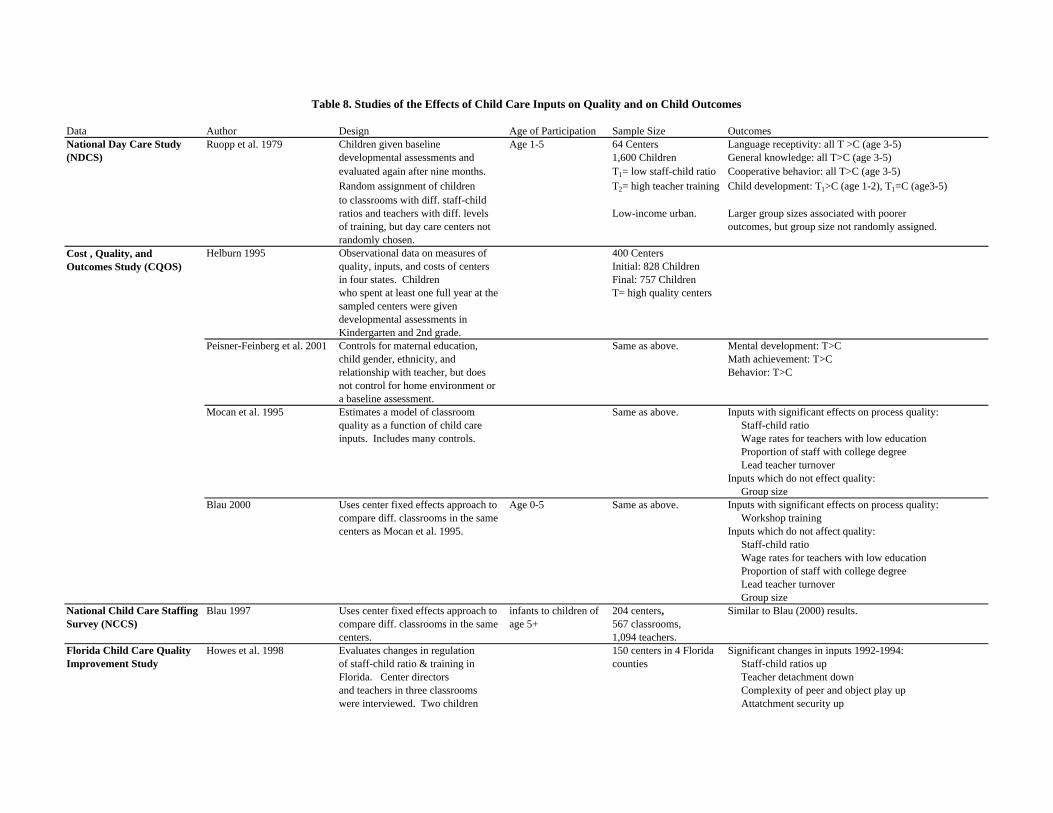
Data Author Design Age of Participation Sample Size OutcomesNational Day Care Study Ruopp et al. 1979 Children given baseline Age 1-5 64 Centers Language receptivity: all T >C (age 3-5)(NDCS) developmental assessments and 1,600 Children General knowledge: all T>C (age 3-5)
evaluated again after nine months. T1= low staff-child ratio Cooperative behavior: all T>C (age 3-5)Random assignment of children T2= high teacher training Child development: T1>C (age 1-2), T1=C (age3-5)to classrooms with diff. staff-childratios and teachers with diff. levels Low-income urban. Larger group sizes associated with poorer of training, but day care centers not outcomes, but group size not randomly assigned.randomly chosen.
Cost , Quality, and Helburn 1995 Observational data on measures of 400 CentersOutcomes Study (CQOS) quality, inputs, and costs of centers Initial: 828 Children
in four states. Children Final: 757 Childrenwho spent at least one full year at the T= high quality centerssampled centers were given developmental assessments inKindergarten and 2nd grade.
Peisner-Feinberg et al. 2001 Controls for maternal education, Same as above. Mental development: T>Cchild gender, ethnicity, and Math achievement: T>Crelationship with teacher, but does Behavior: T>Cnot control for home environment ora baseline assessment.
Mocan et al. 1995 Estimates a model of classroom Same as above. Inputs with significant effects on process quality:quality as a function of child care Staff-child ratioinputs. Includes many controls. Wage rates for teachers with low education
Proportion of staff with college degree Lead teacher turnoverInputs which do not effect quality: Group size
Blau 2000 Uses center fixed effects approach to Age 0-5 Same as above. Inputs with significant effects on process quality:compare diff. classrooms in the same Workshop trainingcenters as Mocan et al. 1995. Inputs which do not affect quality:
Staff-child ratio Wage rates for teachers with low education Proportion of staff with college degree Lead teacher turnover Group size
National Child Care Staffing Blau 1997 Uses center fixed effects approach to infants to children of 204 centers, Similar to Blau (2000) results.Survey (NCCS) compare diff. classrooms in the same age 5+ 567 classrooms,
centers. 1,094 teachers.Florida Child Care Quality Howes et al. 1998 Evaluates changes in regulation 150 centers in 4 Florida Significant changes in inputs 1992-1994:Improvement Study of staff-child ratio & training in counties Staff-child ratios up
Florida. Center directors Teacher detachment downand teachers in three classrooms Complexity of peer and object play upwere interviewed. Two children Attatchment security up
Table 8. Studies of the Effects of Child Care Inputs on Quality and on Child Outcomes

from each class were randomly Inputs which did not change 1992-94:selected for developmental Teacher sensitivityassessments. Process conducted Teacher harshnessbefore regulations changed in 1992 Overall classroom qualityand again in 1994 and 1996. Behavior problemsNo comparison group and no way Cognitive developmentto isolate changes resulting from Significant changes in inputs 1994-1996:regulations. Different children Teacher responsiveness upassessed in each wave. Teacher detatchment up
Attatchment security upInputs which did not change 1994-96: Overall classroom quality Behavior problems Cognitive development
NICHD Study of Early Child U.S. Department of Health Monitors children from birth in 1991 1,300 ChildrenCare (SECC) and Human Services 1998 until present. Selected healthy births English-speaking
to English-speaking mothers overage 18 who planned to remain in thestate for one year. Families and childcare facilities of every type were visited periodically. The effects of child care quality on childdevelopment analysed in manystudies by the NICHD Early ChildCare Research Network (ECCRN). See below.
Early Child Care Research Regression model of cognitive Age 15, 24, 36 months Same as above. Cognitive development: T>CNetwork 2000c development. Controls for five T=high quality care
family and child characteristics andsite dummies in addition to the type, Children in non-maternalquantity, and quality of child care. child care at time of
assessment.Early Child Care Research Models behavior problems. Controls Age 24, 36 months Same as above. Caregiver-reported behavior problems: T1<C (age 24 mo.)Network 1998 for family income, psychological T1=high quality care Mother-reported behavior problems: T1=C (age 24 mo.)
adjustment of the mother, gender, T2=stable care Non-compliance of children in care: T2<C (age 24 mo.)child temperament, quality of home arrangement Problem behavior: T1<C (age 36 mo.)environment, character of mother-child interactions, and child's Children in non-maternalsecurity of attachment to mother. child care at 24 or 36
months.Early Child Care Research Controls for several family Same as above. Peer interactions: T>CNetwork 2000b characteristics as well as child's T=high quality care
cognitive development, temperament,and mother's sensitivity whenanalyzing peer interactions.

Early Child Care Research Models the effects of child care Age 15, 24, 36 months Same as above. Inputs with significant effects on quality:Network 2000a inputs on child care quality. Group size (age 15, 24 mo.)
Regression controls for site, but not Staff-child ratio (age 15, 24 mo.)child, family, or center characteristics. Caregiver education (age 24, 36 mo.)Only characteristics of room, teacher, Caregiver specialized training (age 15 mo.)and type of child care. Caregiver experience (age 24, 36 mo.)
Early Child Care Research Controls for many home and child Age 54 months Same as above. Cognitive functioning: T>CNetwork and Duncan 2002 characteristics and estimates change T=high quality care
score models.National Longitudinal Began with sample of 12,652Survey of Youth 1979 individuals age 14-21 in 1979. Data(NLSY79) collected annually until the present.
Beginning in 1986, children of samplewomen were given developmentalassessments every other year.
Blau 1999 Analyzes the effect of child care variable, depends N=2,503 to 4,031 Inputs with significant effects on development:inputs on child development. on outcome depending on outcome Group size (wrong sign)Controls for type of care, payment, Generally, inputs small and not sig.time spent in care, and family and Home environment large and sig.child characteristics. Models with and w/o family fixed effects.

Program Dependent Care Tax Credit
Exclusion of Employer-Provided Dependent Care Expenses
Aid to Families with Dependent Children Child Care
Transitional Child Care
At-Risk Child Care Child Care & Development Block Grant
Title XX Social Services Block Grant
Acronym DCTC EEPDCE AFDC-CC TCC ARCC CCDBG TXX-CCYear Began 1954 1981 1988c 1988 1990 1990 1975a
Goal Subsidize employment-related dependent care expenses
Subsidize employment-related dependent care expenses
Facilitate participation in the JOBS program
Help families who recently left AFDC for work maintain self-sufficiency
Help families who need child care in order to work and are at-risk of going on AFDC if child care is not provided.
Provide child care services for low-income families, and improve the overall supply and quality of child care.
Help low-income families achieve self-sufficiency; prevent child neglect.
Original Form Tax deduction Amounts paid or incurred by an employer for dependent care assistance provided to an employee are excluded from the employee’s gross taxable earnings
Open-ended entitlement. Vouchers, contracts, or reimbursement of expenses. No fee for recipients
Same as AFDC-CC; limited to 1 year. Sliding fee for recipients.
Capped entitlement. State match required. Sliding fee for recipients. Income limits set by states.
Block grant to states. No state match. 75% of funds for direct subsidies (income<75% of SMI); 25% for quality improvement and consumer education.
Capped entitlement; population-based distribution to states.
1976: credit replaced deduction.
1981: converted to block grant.
1982: subsidy rate and maximum allowable expenses raised. 1983: added to short form 1040A.
1996: States allowed to transfer up to 10% of TANF funds to TXX.
1988: Required SSN of provider.
Current Form Non-refundable Tax Credit
Same as original Block grant to states that can be used for many social services; 15% of funds on average used for child care.
1996: PRWORA consolidated AFDC-CC, TCC, ARCC, and CCDBG into a single program: the Child Care and Development Fund (CCDF).
Combination discretionary and entitlement block grant. States must meet maintenance of effort and matching requirements for some of the entitlement funds. States may transfer up to 30% of their Temporary Assistance for Needy Families (TANF) block grant funds into the CCDF. States may also use TANF funds directly for child care, without transferring them to CCDF.
Table 9. Summary of the History, Goals, and Provisions of Major Federal Child Care Programs
Major Changes None

Current Eligibility Criteria
Both parents (or only parent) employed.
None, other than being employed by a firm that offers this benefit.
States choose income eligibility. Employment required.
Source: Committee on Ways and Means (1998, 2000); Blau (2001, 2003b).Notes:a. Earlier provisions of the Social Security Act provided federal matching funds to the states for social services.b. Less than two percent of the funds in the food program go to adult care centers.
Family income no more than 85% of SMI, but states can (and most do) impose a lower income eligibility limit. Children < 13. Parents must be in work-related activities.
30% tax credit on expenses up to $4,800 for 2 children for AGI ≤10K; subsidy rate falls to 20% for AGI>28K. Effective 2003, 35% credit on expenses up to $6,000 for 2 children for AGI≤15K
c. Before explicit child care subsidies were added to the AFDC program in 1988, states could choose to disregard from earnings up to $200/month in child care expenses incurred by employed AFDC recipients in determining AFDC eligibility and benefit amounts.
Current Provisions
Up to $5000 per year excludable. Expenses excluded from gross income are not eligible for the DCTC.
Sliding fee scale, but states may waive fees for families below the poverty line. At least 4% of funds must be spent on quality-improvement and consumer education. Child care must meet state licensing and regulatory standards. Contracts or vouchers. Relative care eligible if provider lives in a separate residence.
Child care must meet state regulatory and licensing standards

State
Monthly Income Elig-ibility Level
Income Eligibility
as a percent of State Median Income
Are families at or Below Poverty
required to Pay a Fee?
Minimum Fee (full-time rate)
Maximum Family Fee (full-time rate)
Reimburse-ment Rate for Preschool Age Childa
Implied weekly reimbur-sement rateb
Alabama $1,504 45% Some $2.00 /week $85/week $94/week $94.00 Alaska $3,694 85% Some 3% of cost 100% of cost $800/month $185.00 Arizona $1,909 58% Some $1.00/day + $.50
additional c.$10/day + $5 additional c.
$20/day $100.00
Arkansas $1,533 60% None 0 100% of fee $14.40/day $72.00 California $2,821 75% None $0 $10.10 /day $35.90/day $287.20 Colorado $2,139 52% Some $6/month $237/month + $15
each additional c.$18.18 /day $90.90
Connecticutc $3,264 75% Some No fee $326.3 /month $115/week $115.00 District of Columbia
$2,326 62% Some $0 $23.55/day $117.75
Delaware $1,764 44% None 1% of cost 46% of cost $81.40/week $81.40 Florida $1,706 54% All $.80 /day + $.40
each additional c.$9.60/day + $4.80 each additional c.
$102/week $102.00
Georgia $2,817 85% Some $5/week + $3 each additional c.
$52/week + $26 each additional c.
$75/week $75.00
Hawaii $2,874 75% None 0 $75/month $375/month $86.54 Idaho $1,706 54% Some 1% of cost 100% of cost $434/month $100.15 Illinois $1,818 45% All $4.33 (1 c.)
$8.67/month (2 c.)$134.32 (1 c.)
$233.98/month (2 c.)$23.75 /day 118.75
Indiana $2,161 58% None $0 10% of gross income $30/day $150.00
Iowa $1,793 49% None $0 $6/half-day $9.50/half-day $95.00
Kansas $3,114 85% Some $0 $243 /month $2.28/hour 91.2Kentucky $1,851 57% Some $0 $11.50 (1 c.)
$12.75/day (2+ c.)$15/day $75.00
Louisiana $2,420 75% None 0 100% of cost $15 /day $75.00 Maine $3,957 85% Some 2% of income 10% of income $130/week $130.00 Maryland $1,870 40% Some $4/month + $4 per
additional c.$161/month + $122 each additional c.
$407 /month $93.92
Massachusetts $3,869 85% Some $.20/day $22.80/day $29/day $145.00 Michigan $2,172 55% Some $.125/hour $1.75/hour $2.50 /hour $100.00 Minnesota $3,181 75% Some $0 $636/month $44/day $220.00 Mississippi $2,333 85% Some $10.00 (1 c.) $20/
month (2 c.)$155 (1 c.)
$165/month (2 c.)$70/week $70.00
Missouri $1,482 45% Some $1per year $4.00 /day $10/day $50.00 Montana $1,735 57% Some $5 $243 $16.50 /day $82.50 Nebraska $2,105 66% Some $0 $187 (1 c.) $334
/month (2 c.)$16/day $80.00
Nevada $2,798 75% Some 10% of cost of care 100% of cost of care $100/week $100.00
New Hampshirec $1,784 49% Some $0 $.50/week per c. + 34% of daily cost of
care
$16.70 /day $83.50
New Jersey $1,735 37% All $9.10/month + $6.80, 2nd c.
$294.90/month +$156.85, 2nd c.
$21.76/day $108.80
Table 10. Characteristics of State Child Care and Development Fund Plans

New Mexico $2,313 83% Some $11 $191 $346.50/month $79.96
New York $2,338 60% Some $1/week $90/week $30/day $150.00 North Carolina $2,719 75% Some 9% of countable
monthly income9% of countable monthly income
$368/month $84.92
North Dakota $2,445 85% Some 10% of cost of care 80% of cost of care $100/week $100.00
Ohio $2,105 58% All $0 $172/month $100/week $100.00 Oklahoma $1,936 62% Some 0 100% of cost of care $12/day 60Oregon $2,088 55% Some $25 $612 $372/month $85.85 Pennsylvania $2,139 57% Some $5.00 $65 $22.70/day $113.50 Puerto Rico $1,279 85% None $5.00 /month $48/month $160/month $36.92 Rhode Island $2,603 72% None 0 $48 $100/week $100.00 South Carolina $1,446 42% All $3/week $11/week $74/week $74.00 South Dakota $2,140 65% None $10/month 20% copayment $2.00/hour $80.00
$35 (1 c.) $61/week (two c.)
Texas $1,735 52% Some 9% (1 c.) 11% (2+ c.) of gross monthly
income
9% (1 c.) 11% (2+ c.) of gross monthly
income
$20.09/day $100.45
Utah $1,794 56% Some $10 (1 c.) $15 (2 c.) $255 (1 c.) $281 (2 c.) $17.19/day $85.95 Vermont $2,586 83% None $0 $17.03/day $18.92 /day $94.60 Virginia $3,394 85% Some 10% of gross
monthly income 10% of gross monthly
income$42.69/day $213.45
Washington $2,024 54% Some $10.00 $407 $23.41/day $117.05 West Virginia $1,735 60% Some $0 $3.75 (1 c.) $4.50 (2
c.)$17 /day $85.00
Wisconsin $1,909 All $5 (1 c.) $9/week (2 c.)
$63 (1 c.) $78 /week (2 c.)
$5.10 /hour $204.00
Wyoming $1,539 45% All $.05 per hour per c. $.50 per hour per c. $2.14/hour $85.60
Notes: c. stands for “child” or “children.”
a. In most states reimbursement rates vary by location. b. Figures in the last column are calculated from figures in the next-to-last column, assuming 8 hours of care per day, 5 days per week, and 4 and 1/3 weeks per month.
c. Connecticut and new Hampshire did not report information, so figures for these states are from an earlier report. Source: Administration for Children and Families (2001b).
$77/week $77.00 Tennessee $2,027 60% Some $5 (1c.) $9/week (2 c.)

DCTC EEPDCE TXX-CC CCDF
FY1999 2.675 0.995 0.285 9.132FY1998 2.649 0.91 6.399FY1997 2.464 0.862 0.37 4.369FY1996 2.663 0.823 0.352FY1995 2.518 0.792 0.414 3.1
FY1999 6.182 1.76FY1998 6.12 1.515FY1997 5.796 1.248FY1996 6.003FY1995 5.964 1.445
Sources:
Title XX Child Care (TXX-CC): Committee on Ways and Means (2000, p. 600, 634): 15% of $1.9 billion for 1999;13% of $1.775 billion for 2000; Committee on Ways and Means (1998, pp. 714, 720): 14.8 percent of $2.800, $2.381, $2.500 for FY95, 96, 97.
Child Care and Development Fund (CCDF): Expenditure:1997-1999: We computed expenditure figures by summing all federal and state expenditures on the CCDF, either directly or through transfers to TANF, using data from the Annual TANF Reports to Congress (U.S. Department of Health and Human Services, various years) and reports from the Administration for Children and Families (various years). The latter source provides allocations to the CCDF for FY2000 and 2001, but there are no data available on transfers from TANF for these years. Transfers to TANF constituted about half of CCDF spending in FY1999. 1995: U.S. General Accounting Office (1998, p. 4): total funding for thefour programs later consolidated in to the CCDF: AFDC-CC, TCC, ARCC, CCDBG. Children served: 1999: Administration for Children and Families (2000); 1998: Administration for Children and Families (2001a); 1997: Administration for Children and Families (1998); 1995: Administration for Children and Families (1995).
Dependent Care Tax Credit (DCTC): Committee on Ways and Means (2000, p. 816), except 1999: Internal Revenue Service (2001). Figures in the lower panel are number of returns filed claiming the credit, not the number of children.
EEPDCE : Office of Management and Budget, Budget of the United States Government Fiscal Year 1997. These figures are for the calendar year. The method used to compute them is unclear, and in budget statements for subsequent years they are different. They are also different in the Joint Committee on Taxation, JCS-13-99. These are probably the least reliable figures in the table.
Federal + State Expenditures (billions of current dollars)
Children Served (millions)
Table 11. Federal and State Expenditures and Children Served by Major Child Care Subsidy Programs
Notes: See Table 9 for definition of the program acronyms. Expenditures are given in current dollars to facilitate checking with the original sources. To convert expenditures to 2001 dollars using the Consumer Price Index, multiply dollar figures for 1995-2000 by 1.162, 1.129, 1.103, 1.0865, 1.063, and 1.028, respectively.

Annual Household Income ($000)
Proportion with Subsidy
All 0.021 Subsidy No subsidy Subsidy No Subsidy0-4.999 0.04 Center 0.45 0.05 0.41 0.055.0-9.999 0.053 Nonrelative 0.44 0.1 0.33 0.1110-14.999 0.042 Other Nonparent 0.1 0.31 0.2 0.315-19.999 0.029 Pay for care 0.42 0.1 0.46 0.1420-24.999 0.033 Cost/hour 2.55 1.76 2.81 3.0725-29.999 0.025 Mother employed 0.61 0.28 0.79 0.49
30-34.999 0.029 Hours worked if >0
39 33 37 37
35-39.999 0.013 Wage rate 6.62 6.58 6.71 7.140+ 0.009 Annual earnings if
>010,760 7,575 11,053 11,953
Educ.>12 0.45 0.18 0.52 0.32Receives PA 0.112 Married, spouse
present0.12 0.12 0.35 0.51
does not receive PA 0.022 Other adults in household
0.09 0.28 0.17 0.21
# Kids < 5 1.09 0.72 0.84 0.68Black 0.34 0.4 0.28 0.21Hispanic 0.23 0.29 0.17 0.24White 0.43 0.25 0.52 0.5
Sample size 15,747 89 762 88 3,875
Source: Tabulations from the Survey of Income and Program Participation, Spring 1999.
Table 12. Incidence of Child Care Subsidy Receipt and Characteristics of Recipients, 1999
Notes: Unit of analysis is a child. Figures are weighted by the child’s sample weight. A child is coded as receiving a subsidy if the mother reports that a government agency helps pay for child care, or one of the child’s arrangements is Head Start. Public assistance includes cash (TANF, General Assistance, and SSI) and food stamps. Center care includes nursery, preschool, and Head Start. Nonrelative care includes family day care homes, nannies, babysitters, and other nonrelatives except centers.
A. Incidence B. Characteristics of Households with Annual Income < 25,000
Receives public assistance Does not receive public assistance
Public assistance status

Study Data Population Subsidy Method IdentificationEffect of subsidy receipt on employment
Berger and Black (1992)
survey of single mothers in Kentucky; CPS, May 1988
single, child mean age 3.6
Title XX centers only probit for employment before and after subsidy receipt/waitlist
Before-after sub./waitlist comparison
8.4 to 25.3 pp increase, depending on whether "waitlist effect" is included.
Blau and Tekin (2003)
NSAF, 1999 single, child<13
assistance with child care expenses from govt. agency
Two stage Least Squares Linear probability model
county dummies 32 pp increase
Gelbach (2002) 1980 U.S. Census single, youngest child age 5
Kindergarten 2SLS LPM eligibility for Kindergarten (quarter of birth dummies)
4-5 pp increase for both single and married mothers
Meyers, Heintze, and Wolf (2002)
Survey of California AFDC recipients in 4 counties, 1995
single, child<14
assistance with child care expenses from govt. agency under several subsidy programs
Probits for non-parental child care use & subsidy receipt. Predicted value included in probit for employment.
knowledge of child care subsidy system excluded from employment probit.
increase in prob. of subsidy receipt from 0.0 to 0.5: 52 pp increase
Table 13. Studies of the Effect of Child Care Subsidies on Employment

State
CSR GS CSR GSAL 6 6 20 20 1 6 1AK 5 10 NA 8 4AZ 5 15 1.3 5 1AR 6 15 3 10 6CA 4 12 12 sem. hours ECE or rel. field 1 6 1CO 5 10 12 24 0.5 6 2CT 4 8 10 20 0.5 6 1DE 4 8 15 60 hours training in ECE and 1
year experience2 6 1
DC 4 8 10 20 9 credit hours in ECE and 1 year experience
2 5 1
FL 4 20 30 clock hours training in ECE 4 10 1GA 6 12 18 36 10 clock hours training within 1
year after hire2 4 3
HI 4 6 16 Bachelor’s degree; 12 credits in ECE; 6 months experience.
2 6 1
ID 6 12 0.5 6 1IL 4 12 10 20 6 credits in ECE 1.3 12 4IN 4 8 12 1.5 12 6IA 4 12 3 6 1KS 3 9 12 24 12 credits ECE & 6 mo. exper. 1 3 1KY 5 10 14 28 2 10 4LA 6 16 2 6 1ME 4 12 10 30 1 8 3MD 3 6 10 20 6 semester hours in ECE 1 8 1MA 3 7 10 20 HS voc. program in child care 1.5 6 1MI 4 12 1.5 6 1MN 4 8 10 20 24 college credits in ECE & 2
years experience1 10 1
MS 5 10 16 16 3 5 6MO 4 8 10 2.5 10 5MT 4 10 8 hours ECE training in first year
of empl.2.3 6 3
NE 4 12 2 8 4NV 6 13 3 hrs. ECE training in first 6 mo. 3 6 5NH 4 12 12 24 72 hours of workshops 1.3 9 1NJ 4 20 15 20 15 child-related college credits 1.3 5 1NM 6 12 3 6 5NY 4 8 8 16 1.5 6 3NC 5 10 20 25 1 5 3ND 4 10 3 7 4OH 5 12 12 28 2.5 6 1OK 4 8 15 30 3.5 7 1OR 4 8 10 20 2 10 4PA 4 8 10 20 2 6 4RI 4 8 10 20 Bachelor’s degree & meet
standards for RI ECC2 4 4
SC 6 18 2.5 6 1SD 5 20 10 20 2 12 1TN 5 10 15 20 4 7 5TX 4 10 20 35 8 hours ECE training 1 6 1UT 4 8 15 25 3 6 4VT 4 8 10 20 30 hour ECE course in first 6 mo. 2 6 2VA 4 16 2 8 6WA 4 8 10 20 1.3 12 1WV 4 12 0.5 6 4WI 4 8 13 24 80 hours ECE training 2.5 8 4WY 5 15 2 6 3
Table 14. Selected State Child Care Regulations
Sources: The Center for Career Development in Early Care and Education at Wheelock College, 1998; U.S. General Accounting Office (2000a); www.nccic.org/statepro.html; Joseph Hotz and Rebecca Kilburn.
Notes: Blank cell indicates no regulation. ECE = Early Childhood Education. ECC = Early Childhood Certification.. GS = Group Size. CSR = Child Staff Ratio. NA indicates the information is not available.
Day Care CentersFamily Day Care
Homes
Infants Four year oldsPre-Service Education, Experience, and Training Requirement for Teachers
Number of Annual Inspections CSR
Minimum Size for Licensing

Author Data Design Sample Size OutcomesChipty and Witte (1997) 1990 Profile of Child Care
Setting (PCS)PCS data merged to 1990 Census and state and local regulations. Random effect probit estimation to account for unobserved market specific heterogeneity
945 market-oriented centers
Lower required child:staff ratios for preschool children reduce the probability that child care centers care for preschool children rather than school age children, and vice-versa.
Blau (2003c) Data from SIPP merged to state-level data on child care regulation. Estimates include state fixed effects.
17,370 families with at least one preschool age child
Currie and Hotz (2001) NLSY NLSY data merged to state-level data on child care regulations. Multinomial logit estimation of choice of child care on state child care regulations.
44,369 quarters of child life, from 3,394 mothers and 6,290 children.
Regulations are associated with lower probabilities of using regulated child care services. Regulating education of caregivers improves child safety.
Hotz and Kilburn (1997)
National Longitudinal Survey of the High School Class of 1972 (NLS72)
NLS72 data merged to state-level data on child care regulations.
Stricter child:staff ratio and training regulations are associated with lower rates of use of non-parental child care and lower hours of care per week among users.
Hofferth and Chaplin (1998)
1990 National Child Care Survey (NCCS)
NCSS data merged to data on county and state level demographics and regulatory requirements.
1,206 children under 6 whose mothers are working, in training or in school.
Stricter child:staff ratio and training regulations are associated with lower rates of use of non-parental child care and lower hours of care per week among users.
Ribar (1992) Survey of Income and Program Participation (SIPP)
SIPP data merged to data on state-level regulations.
3,738 married families with at least one child under the age of 15
no impact of a stricter child-staff ratio on hours of child care used
tougher regulations are associated with higher family expenditure per hour of child care among families paying for care.
Tougher regulations are associated with higher family expenditure per hour of child care among families paying for care.
Table 15. Studies on the Effect of Regulations on Child Care Use
Survey of Income and Program Participation (SIPP) and Current Population Survey (CPS)
Child care regulations are associated with lower probabilities of using regulated child care services, although no impact on price or quality of care was found.
Effects of child care regulations on labor force participation of mothers shows small negative effects, often insignificantly different from zero

Chipty (1995) 1990 National Child Care Survey (NCCS)
NCSS data merged to data on county-level demographics and state-level regulatory requirements. OLS estimation of reduced forms on equilibrium price, hours and staff/child ratio for family day care and day-care centers.
family day care : 67 day-care centers: n.a.
Blau (1993) Current Population Survey (CPS), March Public Use Tape for 1977-87
CPS data merged to data on state and federal child care subsidy parameters and regulations.
15,195 women between the ages of 18 and 64, consisting of 4,305 child care workers, 7,180 other workers and 3,710 nonworkers.
effects of child care regulations on labor force participation of mothers shows small negative effects, often insignificantly different from zero
mixed results on the effects of regulations on use of child care. stricter group size regulation in both family day care and centers raises family expenditure per hour in both settings, but a stricter child-staff ratio regulation reduces expenditure in both settings. Imposing a training requirement in a given sector is associated with lower family

Program Nameb Program Description Age of Participation Sample Sizec Outcomesd
Carolina Abecedarian Preschoolers: Entry 6 weeks to 3 months Initial: T=57, C=54 IQ: T>C at age 12, T=C at age 15(Campbell & Ramey (1994)) full-day child care Exit: 5 to 8 years Age 8: T=48, C=42 Achievement tests: T>C at ages 8, 15, 21(Campbell et al School age: parent program Age 15: T=48, C=44 Special education: T<C at age 15 (unpublished)) Age 21: T=53, C=51 Grade retention: T<C at age 15
School dropout: T<C at age 21College attendance: T>C at age 21Employment status: T=C at age 21Average age first child born: T>C at age 21
Houston Parent Child Home visits Entry: 1 to 3 years Initial: T=97, C=119 Achievement tests: T=C Development Center Full-day child care Exit: 3 to 5 years Grades 2 to 5: T=50, C=8Grades: T=C(Johnson and Walker Center-based program Bilingual education: T<C (1991))e for parents Special education: T=C
Grade retention: T=CInfant Health and Home visits Entry: birth (home visits) Initial: T=377, C=608 IQ: T>C ages 3,5,8 Development Project Full-day child care 1 year (care) Age 8: T=336, C=538 Behavioral problems: T<C ages 3,5; T=C age 8(McCarton et al (1997))f Exit: 3 years Math achievement: T>C age 8(Hill, Brooks-Gunn and Grade retention: T=C age 8 Waldfogel (2002, in press) Special education: T=C age 8
General health: T=C age 8Milwaukee Project Full-day child care Entry: 3 to 6 months Initial: T=20, C=20 IQ: T>C at grade 8(Garber (1988)) Job and academic training Exit: 5 years Grade 4,8: T=17, C=18 Achievement tests: T=C
for mothers Grades: T=CSpecial education:T=CGrade retention: T=C
Early Training Project Home visits Entry: 4 to 5 years Initial: T=44, C=21 IQ: T=C at age 17(Gray et al (1983)) Summer part-day Exit: 6 years Post High School: T=36, Achievement tests: T=C
preschool program C=16 Special education:T<C, grade 12Grade retention: T=CHigh school graduation: T=C
High/Scope Perry Home visits Entry: 3 to 4 years Initial: T=58, C=65 IQ: T>C at ages 5,7; T=C at ages 8,14 Preschool Project Preschool program Exit: 5 years Age 27: T=58, C=63 Achievement tests: T>C at ages 9,14(Schweinhart et al (1993))f High school GPA: T>C
Special education:T=C, grade 12Grade retention: T=C, grade 12High school graduation: T>CPostsecondary education: T=C age 27Arrests: T<C at age 27Employment: T>C age 19, T=C age 27Monthly earnings: T>C at age 27Receive public assistance: T<C age 27Teen pregnancies: T=C at age 19
Table 16. Model Early Childhood Programs with Randomized Designsa

Institute for Home visits Entry: 4 years Initial: T=312, C=191 Special education:T=C Developmental Studies Part-day preschool program Exit: 9 years Grade 7: T=63, C=34 Grade retention: T=C(Deutsch et al (1983)) Parent center school (K-3)
NotesaSee Barnett and Karoly et al for more detailed information about studies described in this table.bPrograms are grouped such that those enrolling children younger than three years old appear first, followed by those enrolling children after age three.cThroughout the table, 'T' refers to treatment group and 'C' refers to control or comparison group.dOutcomes listed as T>C or C>T were statistically significant at the 5% level.eMost recent published document. See Barnett for description of other studiesfSee Karoly et al. for description of earlier studies.

Program Name Study Design Age of Participation Sample Size OutcomesChicago Child-Parent Compared former CPC children Entry: 3 to 4 years Initial: T=684, C=304 Achievement tests: T>C grade 2, T=C grade 8 Center and Expansion with non-CPC children from same Exit: 9 years Post High School: T=513, High school graduation: T>C Program feeder schools C=244(Fuerst & Fuerst (1993))Chicago Child-Parent Compared former CPC children Entry: 3 to 4 years T=837, C=444 School dropout: T<C at age 20 Center and Expansion with similarly poor children Exit: 9 years High school completion: T>C at age 20 Program eligible for CPC but it was Delinquency and crime: T<C at age 17(Reynolds et al (2000)) not offered in neighborhood Grade retention: T<C at age 15(Temple et al (2000)) Special education: T<C at age 18
Proficiency skills test: T>C at ages 14/15ETS Longitudinal Study Compared attenders with children Entry: 4 years T=333, C=313 Achievement tests: T>C grade 1; T=C in grades 2,3 of Head Start who attended other or no Exit: 5 years(Lee et al (1990))a preschools at grade 3
Head Start Family and Studied gains made by Head Start Entry: 3 to 4 years T=1580, no control Achievement tests: T>C Child Experiences children at age 4 or older Exit: 4 to 5 years Other gains cannot be compared to any control Survey(Zill et al (1998))Florida and Colorado Compared attenders (at age 22 in Entry: 3 to 4 years T=290, C=332 Achievement tests: T=C (T<C in Colorado)Head Start 1988) with those who did not Exit: 4 to 5 years Elementary GPA: T=C (T>C in Florida)(Oden et al (2000)) attend any early childhood Middle and high school GPA: T=C
education program and lived in the Special education: T=Csame census tract High school graduation: T=C (T>C for females)
Postsecondary education: T=CEmployed/enrolled at interview: T=CTeen parent status: T=CUse of public assistance: T=CArrests: T=C (T<C for females)Convictions: T=C
NLSCM Head Start Compared difference between Entry: 3 to 5 years T=896, C=911 Achievement tests: T>C (whites only)(Currie & Thomas attended and nonattended siblings Exit: 5 to 6 years Hispanic study: Grade retention: T>C (whites only) (1995, 1999)) with difference between preschool T=182, C=568 Immunization rates: T>C
and nonpreschool siblings at Child height-for-age: T=C various grades Achievement tests: T>C (hispanics only)
Grade retention: T>C (hispanics only)PSID Head Start Compared Head Start participants Entry: 3 to 4 years T=583, C=3502 Grade retention: T=C(Garces et al (2002)) to non participants between ages High school graduation: T=C
18 and 31. Teen pregnancy T=CWelfare T=CArrests T<CCollege T>C
National Evaluation of 17 EHS sites selected to reflect Entry: 0 to 1 year Initial: T=1513, C=1488 Mental Development Index: T>C age 2, 3Early Head Start program approaches and Exit: Age 3 Low Mental Development Index: T<C age 2, T=C age 3(Administration on demographic characteristics of all Vocabulary production score: T>C age 2Children, Youth and EHS programs funded in 1995-96. Sentence complexity score: T>C age 2Families (2002)) Random assignment conducted Percentage combining words: T=C age 2
within each site to compare Vocabulary: T>C age 3
Table 17. Selected Studies of Large-Scale Public Early Childhood Programs

participants with eligible Aggressive behavior: T<C age 2, 3non-participants. Emotional Regulation: T=C age 2, 3
Orientation/engagement: T=C age 2, 3Engagement of parent during play: T=C age 2, T>C age 3Negativity w/ parent during play: T=C age 2, T<C age 3Attention to objects during play: T=C age 2, T>C age 3Child frustration during parent-child task: T=C age 3Engagement of parent during task: T=C age 3Persistence during parent-child task: T=C age 3Low vocabulary score: T<C age 3
Notes: See Barnett and Karoly et al. for more information about the studies described in this table. None of these evaluations were randomized.T' refers to the treatment, and 'C' refers to the control or comparison group. T>C means that the difference was significant at the 5% level.aMost recent published document. See Barnett for description of other studies

State Spending State Spending State SpendingState Program 1987-88 1991-92 1998-99Alabama Preschool Collaboration Project ― ― $690,000Alaska Comprehensive Preschool $197,000 ― ―
Alaska Head Start Program $2,700,000 $5,728,174 $5,489,951 (State-Funded Head Start Model)
total $2,897,000 $5,728,174 $5,489,951Arizona Early Childhood State Block Grant ― $1,500,000 $10,013,423
(PreK component)Arkansas Arkansas Better Chance ― $5,000,000 $10,000,000California* State Preschool Program $35,500,000 $83,335,000 $127,000,000Colorado Colorado Preschool Program $3,204,000 $21,640,000Connecticut School Readiness and Child Care Initiative ― ― $39,000,000
State-Funded Head Start Model $400,000 $400,000 $5,100,000total $400,000 $400,000 $44,100,000
Delaware Early Childhood Assistance Program $189,000 ― $3,600,000 (State-Funded Head Start Model)
District of Columbia Public School Preschool Program $12,200,000 $11,483,850 $14,591,000District-Funded Head Start Model $1,100,000 $1,556,241 $2,570,000
total $13,300,000 $13,040,091 $17,161,000Florida PreK Early Intervention Program $1,600,000 $69,000,000 $97,000,000
State Migrant PreK Program $2,900,000 $3,064,540 $3,295,172State-Funded Head Start Model ― $6,000,000 ―
total $4,500,000 $78,064,540 $100,295,172Georgia PreK Program for Four-Year-Olds ― ― $217,000,000Hawaii Preschool Open Doors ― n/a $2,700,000
State-Funded Head Start Model $291,790 $529,700 $3,087,387total $291,790 $529,700 $5,787,387
Illinois Early Childhood Block Grant $12,700,000 $71,500,000 $136,000,000 (PreK component)State-Funded Head Start Model ― $500,000 ―
total $12,700,000 $72,000,000 $136,000,000Iowa Comprehensive Child Development Program ― $4,958,315 $7,633,087
("Shared Visions")Kansas Four-Year-Old At-Risk Children Preschool Program ― ― $3,000,000
State-Funded Head Start Model ― ― $2,500,000total $5,500,000
Kentucky Kentucky Preschool Program $232,123 $30,595,270 $39,700,000Louisiana Preschool Block Grant $1,800,000 $3,501,500 $6,650,000Maine Two-Year Kindergarten $27,730 n/a $1,300,000
State-Funded Head Start Model $1,900,000 $2,407,393 $2,329,000Early Childhood Demonstration Grants ― $150,000 ―
total $1,927,730 $2,557,393 $3,629,000Maryland Extended Elementary Education Programs (EEEP) $3,300,000 $8,948,914 $19,263,000Massachusetts Community Parnerships for Children $10,300,000 $7,500,000 $78,500,000
State-Funded Head Start Model $4,500,000 $6,000,000 $6,900,000total $14,800,000 $13,500,000 $85,400,000
Michigan Michigan School Readiness Program $2,300,000 $32,917,700 $67,083,000Minnesota Learning Readiness ― ― $10,300,000
State-Funded Head Start Model $2,000,000 $6,500,000 $18,400,000total $2,000,000 $6,500,000 $28,700,000
Missouri* Missouri Preschool Project ―Nebraska Early Childhood Projects ― ― $500,000New Hampshire NH Head Start-State Collaboration ― $201,000 $230,000
(State-Funded Head Start Model)New Jersey Early Childhood Program Aid $7,900,000 ― $70,000,000
(PreK component)State Equalization Aid for Four-Year-Old Kindergarten ― $9,500,000 ―
Table 18: State Spending on PreK Initiatives

Urban PreK Pilot Program/Good Starts ― $2,500,000 ―State-Funded Head Start Model ― $1,300,000 $1,400,000
total $7,900,000 $13,300,000 $1,400,000New Mexico Child Development Program ― $145,106 $1,300,000
State-Funded Head Start Model ― ― $5,000,000total $145,106 $6,300,000
New York Universal PreK ― ― $67,000,000Experimental PreK $27,000,000 $47,000,000 $50,200,000
total $27,000,000 $47,000,000 $117,200,000North Carolina* Smart Start ― ―Ohio Public School Preschool $18,000 $13,386,236 $17,900,000
State-Funded Head Start Model ― $19,878,559 $92,562,977total $18,000 $33,264,795 $110,462,977
Oklahoma Early Childhood Four-Year-Old Program $832,275 $2,132,120 $36,500,708Head Start State-Appropriated Funds ― ― $3,316,918 (State-Funded Head Start Model)
total $2,132,120 $39,817,626Oregon Oregon Head Start PreK $1,100,000 $8,200,000 $16,272,167
(State-Funded Head Start Model)Pennsylvania* Education Aid for Kindergarten for Four-Year-Olds $1,700,000 n/a $5,700,000Rhode Island* State-Funded Head Start Model $365,000 $1,958,558 $1,965,000
Early Childhood Investment Fund ― ― ―Legislative Allocations for Special Projects ― $200,000 ―
total $365,000 $2,158,558 $1,965,000South Carolina Early Childhood Program $10,900,000 $15,163,447 $22,356,688
(Half-Day Child Development Program)Tennessee Tennessee Early Childhood Education Pilot Program ― ― $3,100,000Texas Public School PreK $46,200,000 $181,000,000 $235,000,000Vermont Early Education Initiative $500,000 $1,414,000 $1,315,000Virginia Virginia Preschool Initiative ― ― $23,500,000Washington Early Childhood Education & Assistance Program $4,700,000 $17,190,000 $28,897,592
Head Start State Match Program $660,000 $530,763 $470,000 (State-Funded Head Start Model)
total $5,360,000 $17,720,763 $29,367,592West Virginia Public School Early Childhood Education $258,574 $1,035,006 $6,232,702Wisconsin Four-Year-Old Kindergarten $4,300,000 $5,800,000 $19,800,000
State-Funded Head Start Model ― $2,250,000 $4,950,000total $4,300,000 $8,050,000 $24,750,000
All States total $202,600,000 $697,065,392 $1,675,455,100
Source: 1987-88 data from Marx and Seligson (1988). 1991-92 and 1998-99 from Children's Defense Fund (1999).
Notes: California: The data presented here is for 1997-98.
Pennsylvania: The data presented for the Education Aid for Kindergarten for Four-Year Olds is for 1997-98.
Missouri: The Missouri Preschool Project was introduced in 1998-99, but the first year of funding (estimated to be $9.2 mill.) was 1999-00.
North Carolina: Total state funding for Smart Start was $140 mill. but the program supports a range of services and it cannot be determined how much of the total was spend on preK.
Rhode Island: The Early Childhood Investment Fund provided $5.3 mill. of funding for a range early childhood-related programs including preK, but no funds were used for this purpose.

Report Study Design Definition of Self-Care Age of Participation Sample Sizea Outcomesb
Aizer (2003) Uses OLS, family fixed effects, and IV Child responds that Age 10-14 Final: 5,838 Skipping school: T>Cestimation to look at self-care in the there is not usually an T=1,518 (self-care) Using alcohol or drugs: T>Cthe NLSY79 Child-Mother file through 1998. adult present when they C=4,320 (supervised) Stealing: T>C
return from school. Hurting Someone: T>CGalambos & Maggs (1989)c No random assignment. Same definition as 6th Grade Final: 112 Peer involvement: all T>C
Students answered a questionnaire to Steinberg (1986) T1= Unsup at friends Problem behavior:T2, T3> T1, C (girls only)determine what category of care they were in. T2= Unsup at home Impulse control: T2, T3< T1, C (girls only)No discussion of methodology. T3= Unsup "hanging Ability to cope: T2, T3< T1, C (girls only)
out"C= Supervised (by parent or ASP)
Marshall et al. (1997) Grade 1 through 4 children recruited from 30 Boston public schools and 8 parochial schools. Data collected through face-to-face interviews and questionnaires with the parent and through observations at the child's after-school setting. OLS regression of the child's behavioral problems on the types of care.
any time spent alone or only with siblings and no adult.
1st-4th grade Final: 181 self care negative effects for poor children
McHale et al. (2001) a short-term longitudinal study with 2 year interval for famlilies who responded to a recruiting letter. Children's behavior evaluated and reported by the parent through home interviews. Children's time use reported by the children and collected through telephone interviews.
Time alone, or with unsupervised peers
10 and 12 Final: 198 T1=time alone T2=w peers
depression: T1>C behavior problems: T2>C
Pettit et al. (1997) A longitudinal study of children (and families) recruited at the time of kindergarten preregistration and observed through grade 7. Data collected through telephone interviews with children (on after-school time use), mother interview (on parental monitoring) and teacher rating (on children's behavior)
time spent alone or with siblings
6th grade Initial: 585 T1=self care in grade 1 or 3 T2=self care in grade 5
grades T1<C, T2=C achievement test scores T1<C, T2=C significant interactions T1 and poverty, behavior problems in Kindergarten.
Pettit et al. (1999) same as Pettit et al. (1997) Time spent unsupervised in 6th grade
7th grade Final: 342 T1=w peers T2=alone T3=w siblings
externalizing problems T1>C, greatest effects for students with low parental monitoring and unsafe neighborhoods, T2=C, T3=C
Richardson (1989) Eighth grade students in 169 classrooms in LA More than 11 hours of 8th Grade Final: 4,932 Cigarette use: T>Cand 67 classes in San Diego filled out a survey self-care per week. T=1,411 (self-care) Alcohol use: T>Con their supervision and substance abuse. C=3,521 Marijuana use: T>CCalculated relative risks of substance abusefor those with more than 11hrs of self care vs. those with 0 hrs of self-care (calculated the ratio of the propotion of kids in each group who abused also stratified bycovariates).
Table 19. Studies of the Effects of Self-Care on Child Outcomes

Rodman et al. (1985) Matched kids in self-care with those in Children who report that 4th & 7th Grade Final: 96 Self-esteem inventory: T=C, 4th & 7th adult care by age, sex, race, family they usually go home 4th Grade: Personal reaction (self-control): T=C, 4th & 7thcomposition, and father's occupation. after school and T=26, C=26 Behavior problems: T=C, 4th & 7thWell-matched on these characteristics. Only either no one or only a 7th Grade:difference between groups is mother's younger sibling at is at T=22, C=22employment and no difference in parental home. Adult carepermission to participate. No random assign. children were those whoUsed child interviews, tests, and teacher reported an adult was atsurveys. T-tests for differences in means. home.
Steinberg (1986) Uses existing data set on Madison, WI Categorization based on 5th-9th Grade Final: 768 Susceptibily to peer pressure: T1=C1 d
school district. ANOVA and ANCOVA child's response to T1=177 Unsup at home all T>all C (girls)(controlling for age, SES, famiy structure, and "where you usually go T2=85 Unsup at friend's all T=all C (boys)mother's employment). Survey includes after school" and T3=57 Unsup "hanging T1<T2, T3
hypothetical peer pressure situations. "are there adults out"present." C1=243 Sup at home
C2=48 Sup atneighbor or relative'sC3=93 Sup at friend's C4=82 Sup at school
Vandell & Corasaniti (1988) Parents of 349 third-graders in a suburban Parents filled out survey 3rd Grade Final: 150 Peer ratings: T1=C2
Dallas school district filled out surveys with the 4 choices of T1=54 (self-care) Grades: T1=C2
describing type of care. Of these, 150 white after-school care listed C1=26 (center) Standardized test scores:T1=C2, C1<all T & Cstudents were deliberately chosen for study. along with "other." C2=42 (mother care) Conduct grades: T1=C2
Most day-care centers were proprietary. Those who reported C3=25 (other adult) Self-perception: T1=C2
Teacher, parent, peer, and self ratings as well a combination of types Parent ratings: T1=C2
as standardized test scores and grades of care under "other" White suburban. Teacher ratings: T1=C2
analysed with ANOVA, MANOVA, and Duncan were categorized in the Negative peer ratings: C1>T1, C2
post-hoc. Controls for parents' education and type of care used for the Academic grades: C1<all T & Cmarital status. majority of days/week.
Vandell & Ramanan (1991) Used the NLSY79 with data from home visits Parents report "primary" 3rd-5th Grade Final: 390 Headstrong: T>all C (but T=C w/ family controls)of NLSY staff. ANOVA then Duncan's post hoc after school care T=28 (self-care) Hyperactive: T> all C (but T=C w/ family controls)analyses. arrangement. C1=114 (other adult) Anxious: T= all C
C2=248 (mother care) Peer conflicts: T= all CAntisocial: T= all C
Overrepresentative Dependent: T= all Cof single-parent Harter self-rating, Cognitive: T= all Cand low-income. Harter self-rating, General: T= all C
Digit span: T= all CPeabody Picture Vocab. Test: T= all CPeabody Indiv. Achievement Test: T= all C
a Throughout the table, 'T' refers to treatment group and 'C' refers to control or comparison group.b Outcomes listed as T>C or C>T were statistically significant at the 5% level unless otherwise noted.c In Galambos and Maggs (1991).d Steinberg et al. also break the unsupervised group into children whose parents know their whereabouts and those who do not. They find some evidence that those children whose parents know their whereabouts (no matter where they go after school) are less susceptible to peer pressure.

Program Name Program Description Study Design Age of Participation Sample Sizea Outcomesb
RandomGevirtz Homework Project (Cosden et al. 2001)
Homework assistance with a credentialed teacher after school 3 to 4 days per week (no drop-in)
stratified random assignment of 4th graders to treatment and control groups, students followed from 4th-6th grades
4th-6th grade Final: 90 T=36 C=54
No difference between treatment and control. Dosage correlated with achievement.
Howard Street One-on-one adult reading Teachers identify the lowest 50 readers 2nd-3rd Grade Final: 60 Word recognition: T=CTutoring Program tutors work with 20 low in second and third grade. Then kids are T=30, C=30 Basal word recognition: T>C(Morris et al. 1990) reading ability second and ranked according to 3 reading Basal passages: T>C
third graders at a public and spelling tests. The 2 lowest scoring Low SES urban school. Spelling (correct score): T>Cschool. Operates afterschool are paired, then the next two, etc. Spelling (qualitative score): T>C4 days/wk from October-May, and one of each pair is randomly but students attend only assigned to participate in the program.2 days/wk for 50 hrs. of total Study compares students in program totutoring over the year. the control group in each of two years
using the same 3 tests that wereadministered prior to the program.No sig differences between control andtreatment group on tests at pretest.Compared mean gains for T and Cusing t-tests.
Memphis City Schools Goal to improve students' Matched students on the basis of Program: Final: 656 Reading test score: T>C grade 3, T=C grades 2, 4Extended-Day Tutoring reading in grades 1-4 with standardized test scores, then attitude and 1st-4th Grade T=328, C=328Program group tutoring in the after- behavior. One student from each pair Study:(Ross et al. 1996) school hours. Focus on assigned to participate (supposedly 2nd-4th Grade Title I students
reading, with occassional randomly, although 2 outlier schoolswriting, computer, and test- may have assigned students first, thentaking skills. found a match. These 2 (out of 13) hadOne hour a day, 3 days/wk. different mean test scores for T and C and
were left out of the analysis. Study usesstandardized test scores to evaluatestudents. ANCOVA and matched-pairs
Quantum Opportunities After-school educational Entering 9th gr. students whose families 9th-12th Grade Initial: 250 High school graduation or GED: T>C(Hahn, Leavitt & Aaron activities (250 hrs), were on public assistance randomly T=125, C=125 Post-secondary attendance: T>C1994) development activities selected from schools near program Final: 170 Honors/awards: T>C
such as mentoring & peer tut. sites. Then randomly assigned to control T=88, C=82 Attending high school: T=C(250 hrs), community svc. or intervention. Those assigned to the Dropout of High School: T<Cactivities (250 hrs) each year program were then called and encouraged All students from Have Children: T=C (T<C at 10% level)for 4 years. Students recieve to join. Suveys conducted before and families receiving No. of children: T<Chourly bonuses and stipends throughout the 4-year program. Final public assistance. In trouble with police in past year: T=C (T<C at 10% level)
for completing each part of evaluation in autumn after completion. On welfare, AFDC, food stamps: T=Cprogram. Do community service in past 6 mo: T>C
Volunteer mentor/tutor in past 6 mo: T>CStart business or self-employed: T=CFamily life is happy: T=CHopeful about future: T>CDepressed about life: T=C
Table 20. Studies of the Effects of After-School Programs on Child Outcomes

Bothered about things: T=CLonely: T=CLife has been a success: T>CHave future plans: T=CNeed reading/math skill improvements: T=CNeed training for a good job: T=CNeed help finding a job: T=CNeed help with alcohol/drug problem: T<C
Non-randomThe ADEPT Project Comprehensive afterschool Teachers and social workers chose 60 K-6th Grade Initial: 836 Self-esteem: all T<C(Ross et al. 1992) program focusing on building kids at each school site who they T=540, C=296 Depression: all T=C
positive self-esteem and considered to be latchkey. Families T2=self-esteem Risk-taking: all T=Cproviding homework assist. were invited to an orientation and teachers building curriculum Impulsivity: all T=Cand activities for social and then selected 20 to participate based on Final: 667 Sulking: all T=Cemotional growth. Kids "need." Those youths whose parents T=443, C=224 Egotism: all T<Cparticipated in 2 hr. sessions were not interested became the control Learning: all T=Cwith free play, creative group. Quasi-experimental. Use data Mostly low-income Shyness: all T=Cdramatics, and hmwk assist. from parents, teachers, and school African-American Acting: all T=Cthroughout the school year. records. ANOVA with gain scores used. Pressure: T=C, T2<C
Motivation: T=C, T2>CFrustration: T=C, T2<CPeer interaction: T=CStandardized test scores: T=C, T2>C
Boston After School Study (Marshall et al. 1999)
Regular afterschool programs at public and parochial schools in Boston
Grade 1 through 4 children recruited from 30 Boston public schools and 8 parochial schools. Data collected through face-to-face interviews and questionnaires with the parent and through observations at the child's after-school setting. OLS regression of the child's behavioral problems on the types of care.
1st-4th grade Final: 181 Behavior Problems, T<C for "regular attenders"
Extended Services School Initiative (Grossman et al. 2002)
Comprehensive afterschool program seeking to promote the well being and positive development of young people in their out of school hours.
Teachers identify the lowest 50 readers 2nd-3rd Grade Final: 60 T=regular attenders
Word recognition: T=C; skip school: T<C
Kindergarten After- After-school program designed Sociometric interviews and classroom Kindergarten Final: 100 Identified as "friend" by peers: T>CSchool Program to provide a service to working observations used to asses differences in T=30, C=70 Teacher talk to child, spontaneous: T=C(Howes et al. 1987) parents by providing extended social adjustment between participants in Teacher talk to child, responsive: T>C
day care beyond the morning- the after-school program and non- School admissions Teacher talk to child, social: T=Conly kindergarten class. Also participants at the end of one school year. reflect ethnic diversity Teacher talk to child, information: T=Caims to enhance socio- Non-random, but T and C groups had of U.S. Teacher talk to child, directions: T=Cemotional development. similar demographic composition. Teacher talk to child, praise: T=CLocated on school grounds. Chi-square and F tests of means. Teacher talk to child, reprimands: T=COperates 5 days/wk. Children Child talk to teacher, spontaneous: T>Cmay stay until 3 or 5:30pm. Child talk to teacher, responsive: T=C
Child talk to teacher, social: T=CChild talk to teacher, information: T>CChild talk to teacher, demands: T=C

Teacher responsiveness to child, positive: T>CTeacher responsiveness to child, negative: T=CTeacher responsiveness to child, unaware: T=C
LA's BEST Comprehensive after-school 2-year longitudinal study of some Program: Initial: 146 The following outcomes did not have significance tests:(Brooks et al. 1995) program intended to combat participants in the 10 longest-running K-6th Grade T=80, C=66 GPA math: T=C
obstacles to educational LA's BEST sites. These participants Study: Final: 123 Reported effort in math: T=Cacheivement. Academic had attended program for at least 2 yrs, 5th-8th Grade T=69, C=58 GPA reading: T=Ctutoring and instruction, had complete school records, and Reported effort in reading: T=Ccultural enrichment, recreation, parental permission. GPA composition: T=Ccomputer activities, and No random assignment. Comparison Reported effort in composition: T=Cnutrition for K-6th graders group formed from kids in same school GPA social studies: T>Cafter-school until 6pm M-F whose parents agreed to participate. Reported effort in social studies: T>Cin 19 of LA's poorest schools. Comparison group sig. different in grades GPA science: T>C
(higher), family characteristics, and Reported effort in science: T>Cethnicity. Data collected for 1992-93 and1993-94 school years. Compared the improvement in scores of treatment and
The following outcomes were reported as significant (or not) at the 5% level:
controls. Feel that grown-ups in afterschool life care: T=CFeel that grown-ups in afterschool life expect you to do well: T=CFeel that grown-ups in afterschool life are easy to talk to: T=CFeel that grown-ups in afterschool life are helpful: T>CInclude teachers to help with a problem: T>CInclude student aides for help with a problem: T>C Positive attitude toward school: T>CFelt safe during afterschool hours: T>CEducational expectations (how far you will go in school) : T>C c
LA's BEST Same as above. Compares participants to schoolmates 2nd-5th Grade Initial: Language redesignation (English profic): T>C(Huang et al. 2000) who did not participate. Followed T=4312 (grades 4, 6, 8), T=C (grades 5, 7)
students for five years. Broke down C=15010 School absence: T<C (grade 6, 7), T=Cparticipants into those who attended 75% (grades 8, 9)of days (high), 25-74% (med), and less Math acheivement test scores: T=C (butthan 25% (low). started with T<C)Control for gender, ethnic, income, Felt safe after school: T>Cand language status (English profic). Like school: T>CNot random assignment. Engagement in school: T>C
Educational expectations: T>CStandardized math tests: High>LowStandardized reading tests: High>LowStandardized language arts tests: High>LowSchool attendance: High>Low
LA's BEST (Huang et al. 2001)
Surveys 74 of the 76 LA's BEST sites in June 2001. Participants whose parents
2nd-5th Grade Initial: 3,717 Reading SAT-9: Proportion of LA's BEST students scoring above 50th
gave permission (27% of all participants). No control group. Students tested in
National Percentile Rank (NPR) rose by 1 percentage pt.
Same as above.

1998-99 and again in 1999-00. Math SAT-9: Proportion of LA's BEST students scoring above 50th NPR rose by 3 percentage pts.Language arts SAT-9: Proportion of LA's BEST students scoring above 50th NPR rose by 5 percentage pts.
Milwaukee Public School Formal ASP participants were Parents volunteered for the study and 3rd Grade Initial: 216 GPA math: T>C1, C2
District in 8 different programs at 5 216 children were selected if they T=34 Formal ASP GPA reading: T>C1, C2
(Posner & Vandell 1994) elementary schools. 21 kids participated in one of the arrangements C1=121 Maternal care GPA other subjects: T> all Cattended the same on-site for 3 days a week or more. C2=45 Informal adult GPA conduct: T> C1, C2
ASP sponsored by the district Children evaluated with teacher and supervision Wisconsin 3rd grade reading test: T= all Cthat offered academic, parent reports of behavior, the child's C3=15 Self-care Antisocial: T<C2, C3
recreational, and remedial grades, and a standardized reading test. Work habits: T> all Cactivities at the end of the Not random. Low income Peer relations: T> all Cschool day. The other prgms. Chi-sq tests for selection on categorical Emotional adjustment: T>C1, C2
attended typically had a variables lead them to control for race, Adult relations: T= all Crecreational focus with mother's education, and family income. Anxious: T= all Csome optional assisted Use ANCOVA and MANCOVA. Dependent: T= all Chomework time. Then Fisher tests for differences between Hyperactive: T= all CParticipants in all categories T and all C. Time engaged in academic activities: T> all Chad to spend at least 3 Time engaged in enrichment: T> all Cdays per week in these Time watching TV: T< all Carrangements. Time in outdoor unorganized activities: T< all C
Time in transit: T= all CTime eating: T= all CTime in indoor unorganized activities: T= all CTime with adults present: T> all CTime with peers present: T> all CActively engaged with peers: T> all CActively engaged with adults: T> all CActively engaged with siblings: T< all CAcademic activities with adults: T> all C
Milwaukee Public School Same as above. Followed the same children as above 3rd-5th Grade Initial: Same as above. Time on academics: T> all C (grades 3, 4), T= all C (grade 5)
District for 2.5 yrs. Final: 194 Time on non-sport extracurriculars: T> all C (grades 3, 4, 5)
(Posner & Vandell 1999) Used t-tests to contrast the outcomes of kids in formal programs with others.
no diff. attrition Time in outdoor unorganized activities: T< all C (grades 3, 4, 5)
T=26 Formal ASP C1=121 Maternal care
Time in coached sports: T= all C (grades 3, 4), T> all C (grade 5)
C2=30 Informal adult supervision
Time in indoor structured activities: T= all C (grades 3, 4), T> all C (grade 5)
C3=17 Self-care Time watching TV: T< all C (grades 3, 4, 5)Time socializing: T= all C (grades 3, 4), T< all C (grade 5)Time doing chores: T< all C (grades 3, 4, 5)Time in transit: T= all C (grades 3, 4, 5) d
Low income

The Afterschool Corporation (TSAC) (Welsh et al. 2002)
Community-based organizations (CBOs) and other nonprofit organizations are funded by The After-School Corporation (TASC) to operate in-school after-school programs from 3:00 p.m. to 6:00 p.m. Monday through Friday throughout the public school year. TASC programs include educational enrichment through activities in language arts, science, mathematics, fine and performing arts and sports.
Compares the actual changes in academi indicators (performance on standardized tests and school attendance) of TASC participants over a three year period to projected changes for nonparticipants, derived from OLS regressions controlling for factors including prior year's test scores, and demographic and educational background. Data were collected from TASC sites.
K-8th grade T=25,909 C=39,780
gains in math: T>C, especially for students from disadvantaged circumstances. increase in attendance T>C
a Throughout the table, 'T' refers to treatment group and 'C' refers to control or comparison group.b Outcomes listed as T>C or C>T were statistically significant at the 5% level unless otherwise noted.c All outcomes reported are based on Brooks et al.'s "method 1" which compares improvements in test scores of the treatment and control groups (as described above). "Method 2" finds stronger evidence of positive effects of LA's BEST as cited in other meta-analyses. However, method 2 simply excludes low-scoring students from the treatment group, thereby biasing the results. d Posner and Vanell also report the effects that these activities had on GPA, emotional adjustment, work habits, and behavior problems in 5th grade. They find that time spent on unorganized outdoor activities is associated with worse outcomes for whites. Considering this finding in conjunction with the list of results above, suggests that formal afterschool programs may have some positive effects. On the other hand, time in non-sport extracurriculars lowers emotional adjustment among blacks, so to the extent that afterschool programs increase time spent in these types of activities, they may have detrimental effects on student outcomes.

Program Name Program Description Study Design Age of Participation Sample Sizea Outcomesb
Across Agesc,d Mentoring by adults over Random assignment of sixth grade 6th Grade Initial: 729 Increased positive attitudes: T>C(LoSciuto, Rajala, age 55 at least 2 hours/wk, classes in three schools to either program Final: 562 no diff. Inc. knowledge of older people: T>CTownsend & Taylor 1996) community service 1 hr/wk, or control group. Used ANCOVA. Likely to have negative reaction to drug use: T>C
26 sessions of social problem More community service: T>Csolving, wrkshps for parents. School attendance: T>C
Big Brothers/Big Sisters Mentors from the community Randomly assigned eligible youth to Program: Age 5-18 Initial: 1138 Likelihood of initiating drug use: T<C(Tierney, Grossman are matched with eligible treatment or wait list at eight sites with Study: Age 10-16 T=572, C=567 Likelihood of initiating alcohol use: T=C (T<C at 10%)& Resch 1995) youth (typically those with large case loads across the country. Final: 959 No. of times hit someone: T<C
only one adult involved in life). Surveys were administered to parents T=487, C=472 No. of times stole something: T=CMentors are usually required and youth at the time of assignment and No. of times damaged property: T=Cto interact with youth 18 months later (note: those assigned to From single-parent Perceived ability to complete schoolwork: T>C9-12 hours per month for the wait list remained on it for all 18 months). households. GPA: T=C (T>C at 10%)first year. Case managers also completed data No. times skipped class: T<C
collection forms throughout the study. No. of times skipped day of school: T<CInterestingly, 22% of youth in the Weekly hours of homework: T=Ctreatment group were never matched, Weekly hours spent reading: T=Cusually because the youth became School value scale: T=Cineligible or no longer wished to be Overall positive parental relationship: T>Cmatched. This is typical for the program. Improved parental relationships (trust): T>CThe treatment group represents the Improved communication wth parent: T=Copportunity to be matched. Anger/alienation in parental relationship: T=COutcomes were usually based on Number of times lied to parents: T<C e
several survey questions and establishedscales of peer relationships, scholasticcompetence, etc. Used OLS w/ covariatescontrolling for age, race, gender, abuse,home environment, and site. Used logitfor dichotomous outcomes.
I Have a Dream A sponsor adopts a sixth Natural experiment where participants 6th-12th Grade Final: T=92, C=89 High school graduation: T=70.6%, C=35.5% (Kahne & Bailey 1999) grade class and offers are compared to the sixth graders of the College enrollment: T=64.7%, C=18.9% (approx)
long-term financial, academic, previous year (in the same school).and social support including Study focuses on two IHAD programs in No significance tests reported.afterschool programs, Chicago.tutoring, summer programs,and college scholarships.
Teen Outreachc,d 45 hrs of volunteer svc. And 25 schools nationwide randomly assigned 9th-12th Grade Initial: T=342, C=353 School failure: T<C(Allen, Philliber, Herrling weekly small class to treatment or control from 1991 to 1995, Final: T=324, C=323 School suspension: T<C& Kuperminc 1996) discussions of values, but students in those schools elected to Teen pregnancy: T<C
decision making, parenting, participate. Sites with more interested life options. students than could participate heldCan be in-school or after. lotteries. Immediate posttests after
1-year of participation.Woodrock Youth Weekly classes (skills for Classes in 4 Philadelphia schools were Age: 6-14 Initial: 453 Self-esteem: T=C (age 6-9, age 10-14)
Table 21. Studies of the Effects of Positive Youth Development Programs on Child Outcomes

Development Project human relations), daily randomly assigned to treatment or control. T=161, C=292 Relationship w/ and perception of students of(LoSciuto, Freeman, mentoring, peer tutoring, Different pre- and posttests given to Final: 367 other races: T>C (age 6-9), T=C (age 10-14)Altman & Lanphear 1997)c homework assistance, younger children (age 6-9) and older T=130, C=237 Alcohol, tobacco, or drug use in last year:
extracurricular activities, and children (age 10-14). ANCOVA to Age 6-9: n=170 T<C (age 6-9), T=C (age10-14)some home visits. Also, compare outcomes. Age 10-14: n=197 Alcohol, tobacco, or drug use in last month: out-of-school special events. Atrit diffs in age (older T<C (age 6-9, age 10-14)In-school classes once a wk attrited more) and more Negative attitude toward alcohol, tobacco, and and an after-school prgrm. from T group among drug use: T=C (age 6-9), T<C (age10-14)
older and more from Cfor younger. (Note that paradoxically, among the older group,
T had a less negative attitude toward drugs.)
a Throughout the table, 'T' refers to treatment group and 'C' refers to control or comparison group.b Outcomes listed as T>C or C>T were statistically significant at the 5% level unless otherwise noted.c in Catalano et al. (1999)d in Roth et al. (1998)e Other social and behavioral outcomes were also reported, such as self-confidence, social acceptance, conflict with peers, and time spent in cultural activities, but none were significantly different for the treatment and comparison groups.