Overview ta3520 Introduction to seismics

•  Fourier Analysis •  Basic principles of the Seismic Method •  Interpretation of Raw Seismic Records •  Seismic Instrumentation •  Processing of Seismic Reflection Data •  Vertical Seismic Profiles

Practical: •  Processing practical (with MATLAB)

Signal and Noise

Signal: desired Noise: not desired So for reflection seismology: - Primary reflections are signal - Everything else is noise!

Signal and Noise (2)

Direct wave: noise

Refraction: noise

Reflection: (desired) signal

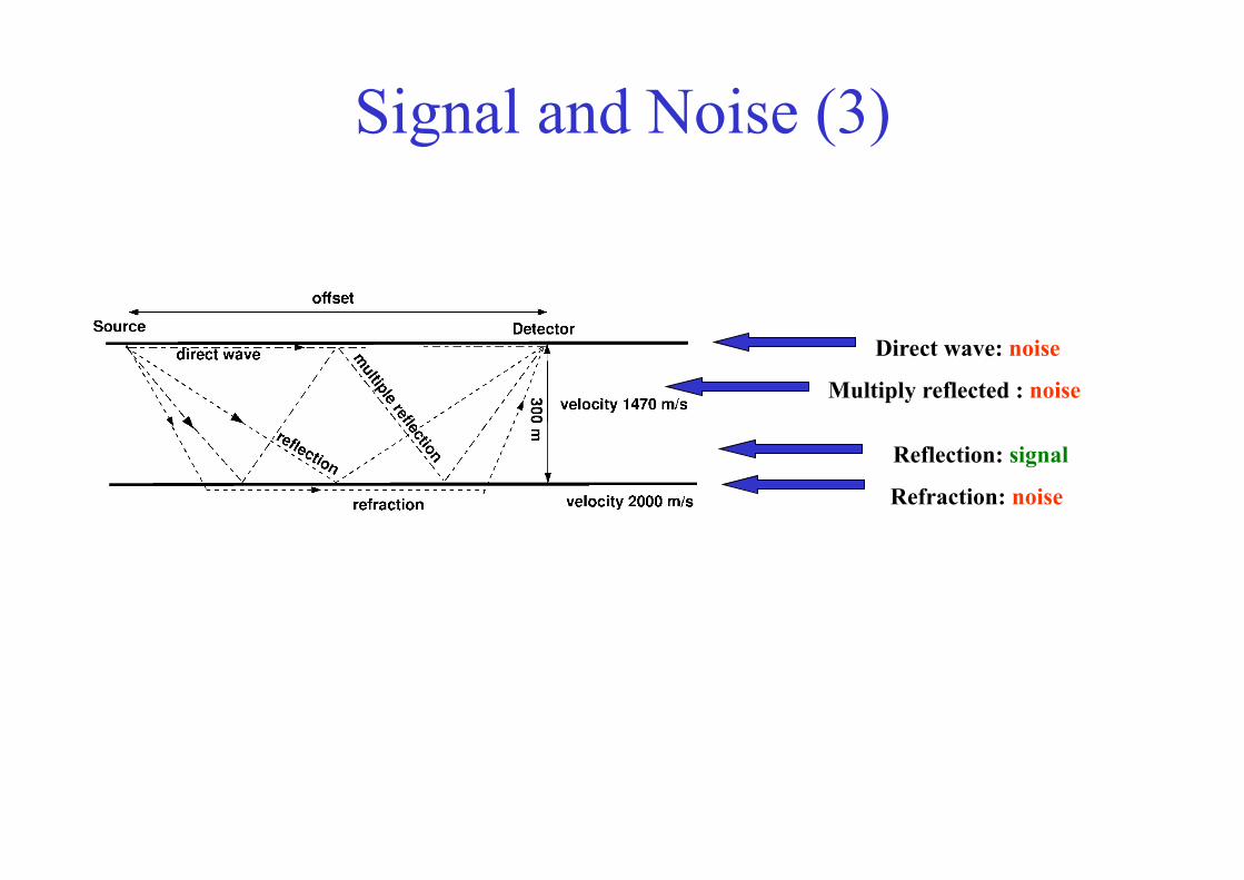
Signal and Noise (3)

Direct wave: noise

Refraction: noise

Reflection: signal

Multiply reflected : noise

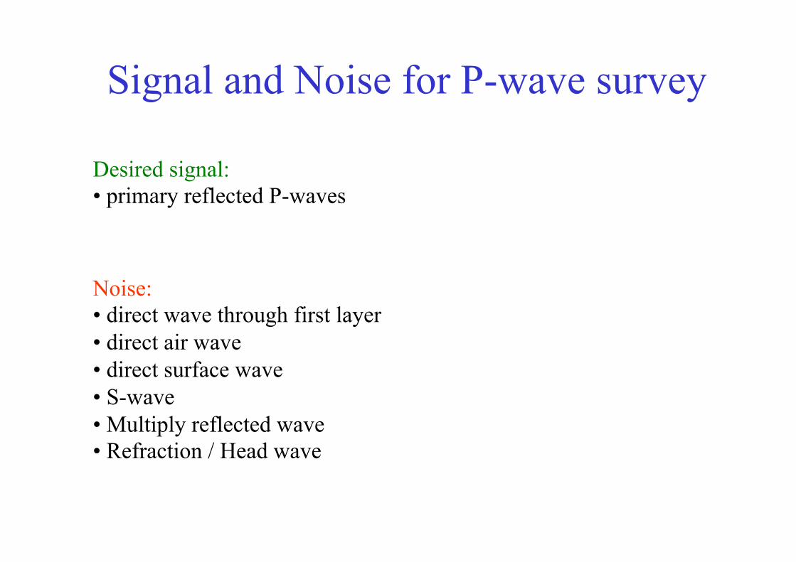
Signal and Noise for P-wave survey

Noise: •  direct wave through first layer •  direct air wave •  direct surface wave •  S-wave •  Multiply reflected wave •  Refraction / Head wave

Desired signal: •  primary reflected P-waves

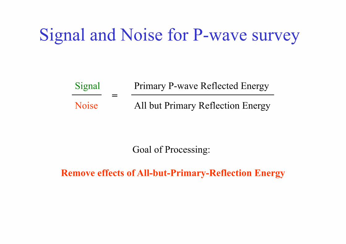
Signal and Noise for P-wave survey

Signal

Noise =

Primary P-wave Reflected Energy

All but Primary Reflection Energy

Goal of Processing:

Remove effects of All-but-Primary-Reflection Energy

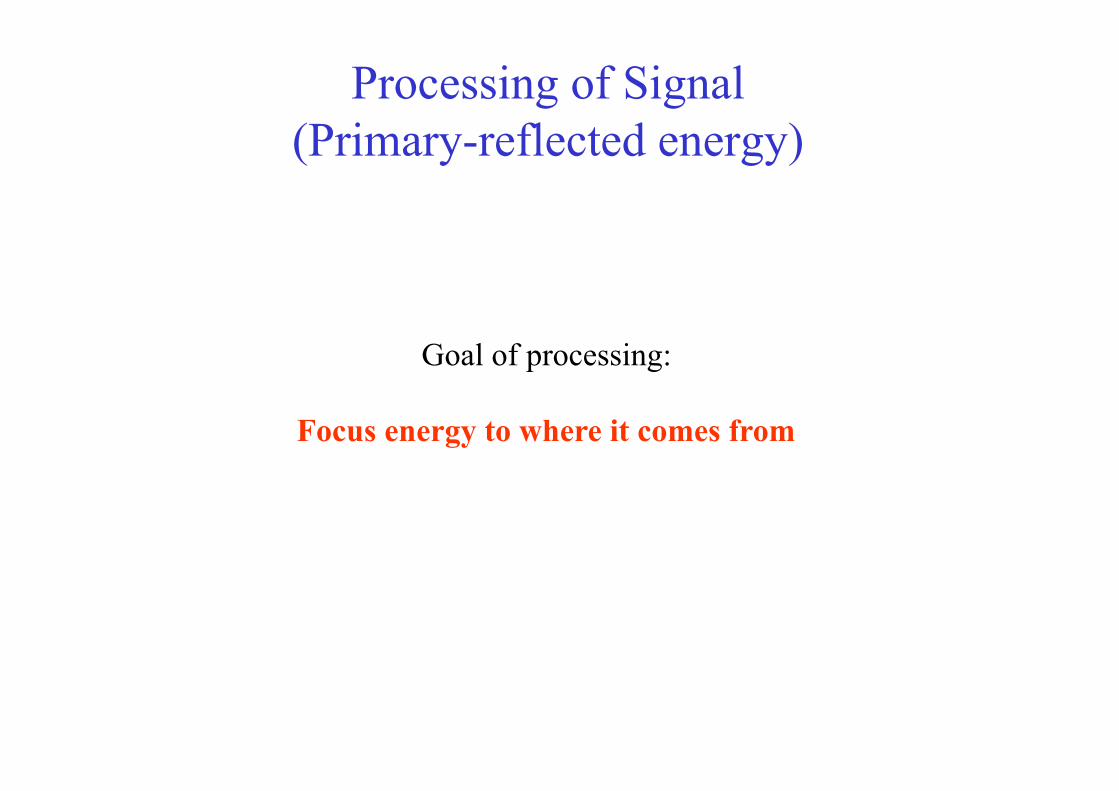
Processing of Signal (Primary-reflected energy)

Goal of processing:

Focus energy to where it comes from

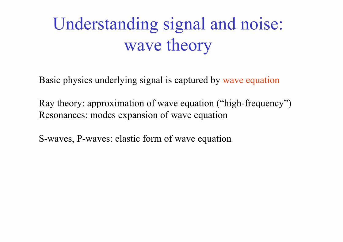
Understanding signal and noise: wave theory

Basic physics underlying signal is captured by wave equation Ray theory: approximation of wave equation (“high-frequency”) Resonances: modes expansion of wave equation S-waves, P-waves: elastic form of wave equation

Seismic Processing •  Basic Reflection and Transmission

•  Sorting of seismic data

•  Normal Move-Out and Velocity Analysis

•  Stacking

•  (Zero-offset) migration

•  Time-depth conversion

Basic Reflection and Transmission

(pdf-file with eqs)

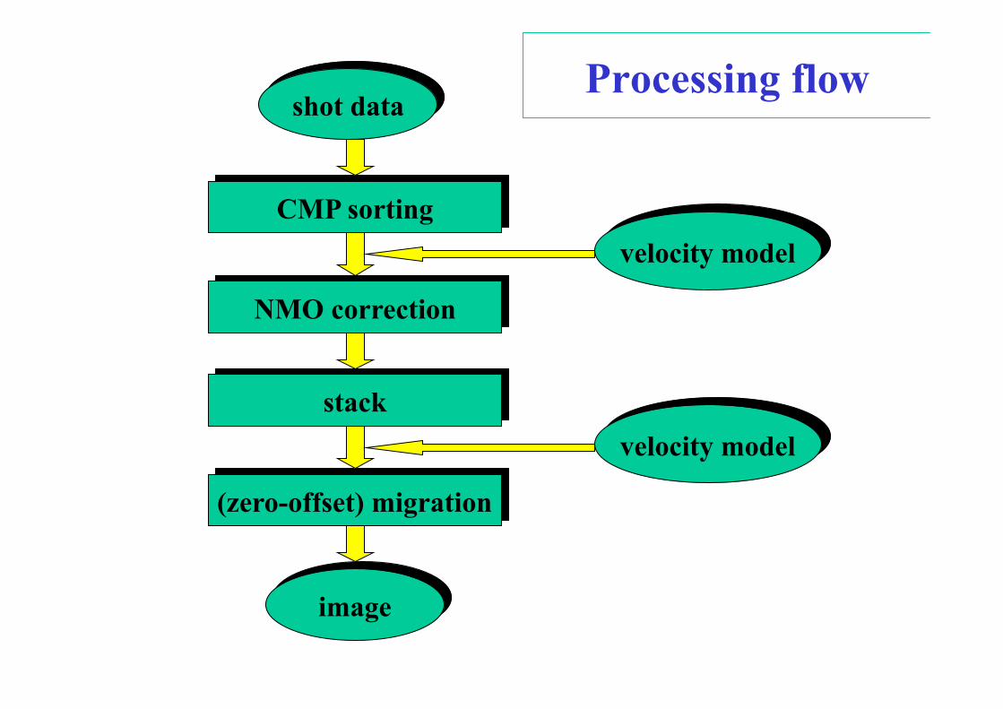
CMP sorting

shot data

image

NMO correction

(zero-offset) migration

stack

velocity model

velocity model

Processing flow

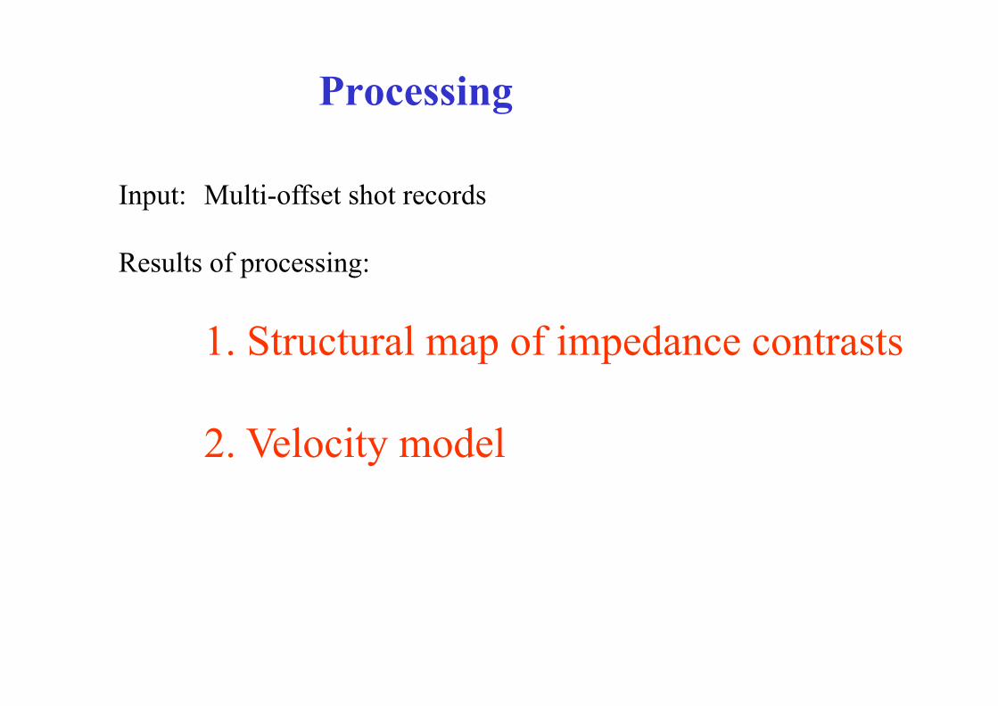
Processing

Input: Multi-offset shot records Results of processing:

1. Structural map of impedance contrasts

2. Velocity model

Sorting: Common Shot gather

Seismic recording in the field: Common Shot data

(Each shot is recorded sequentially) Nomenclature:

- common-shot gather - common-shot panel

Common Shot gather

Sorting: Common Receiver gather

Gather all shots belonging to one receiver position in the field Analysis/Processing: shot variations

(e.g., different charge depths) (Also in common-shot gathers: receiver variations, e.g.,

geophones placed at different heights)

Common Receiver gather

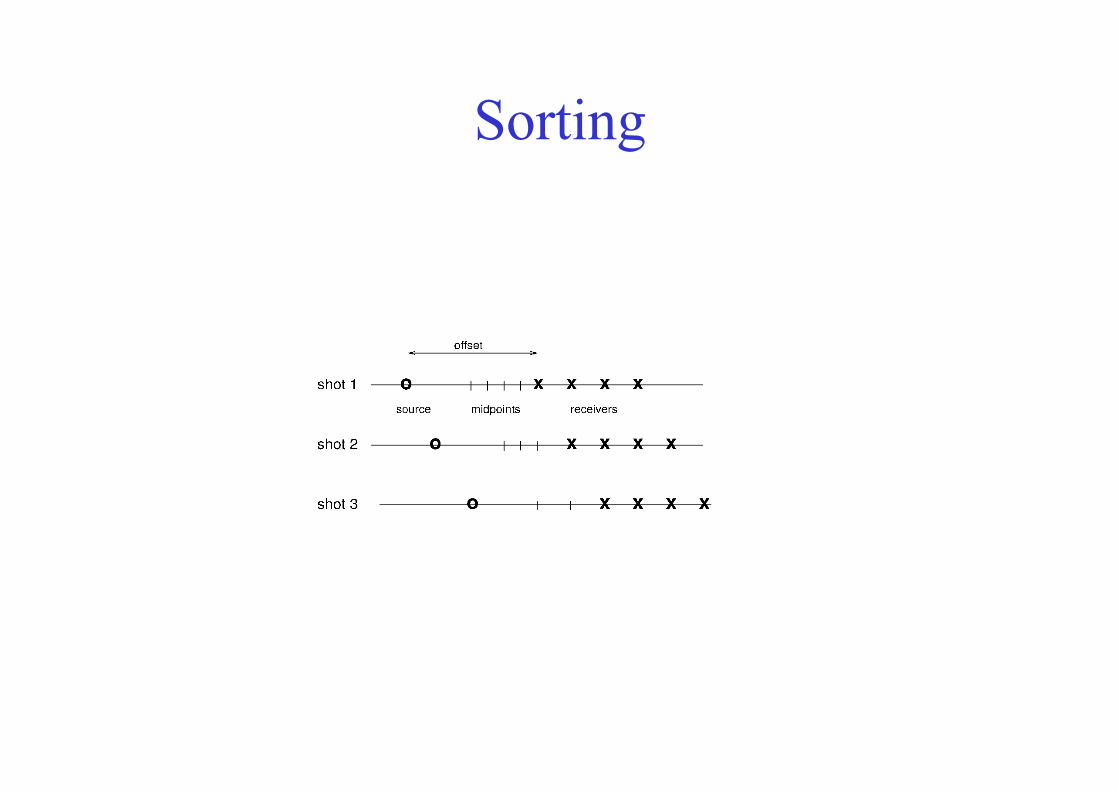
Sorting

Sorting: Common Mid-Point gather

Sorting: Common Mid-Point gather

Mid-points defined as mid-points between source and receiver in horizontal plane Since reflections are quasi-hyperbolic: •  Seismograms not so sensitive to laterally varying structures

•  Good for velocity analysis in depth

•  Stacking successful (noise suppression)

In practice, not really a point but an interval: BIN

CMP gather over structure

Sorting: Common Offset gather

Purpose: •  Very irregular structures (in which stacking does not work)

•  Application of Dip Move-Out (correction for dip of reflector)

•  Checking on migration: small and large offsets should give the same picture : otherwise velocities are wrong

In practice, not really a point but an interval: BIN

Zero-offset gather over structure

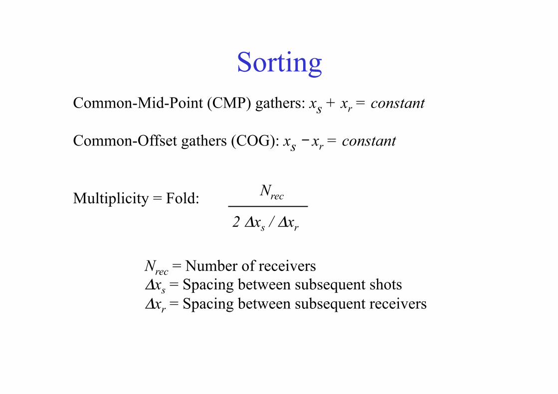
Sorting Common-Mid-Point (CMP) gathers: xs + xr = constant Common-Offset gathers (COG): xs - xr = constant Multiplicity = Fold: Nrec

2 !xs / !xr

Nrec = Number of receivers !xs = Spacing between subsequent shots !xr = Spacing between subsequent receivers

Sorting

CMP sorting

shot data

image

NMO correction

(zero-offset) migration

stack

velocity model

velocity model

Processing flow

Reflection 1 boundary

Normal Move-Out: 1 reflector T = R

c =

(4d2 + x2)1/2

c x = source-receiver distance R = total distance travelled by ray d = thickness of layer c = wave speed

We do not know distance, but we know time:

T = T0 ( 1 + x2

c2 T02

)1/2

where T0 is zero-offset (x=0) traveltime: T0 = 2d/c

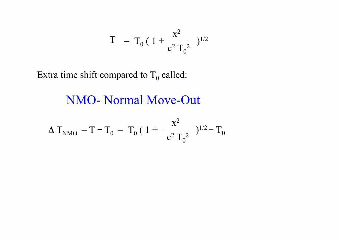
T = T0 ( 1 + x2

c2 T02

)1/2

Extra time shift compared to T0 called:

NMO- Normal Move-Out

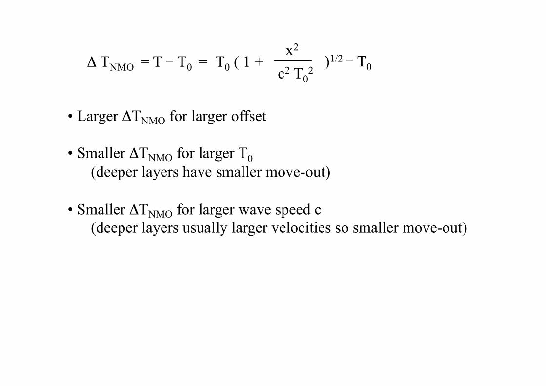
! TNMO = T - T0 = T0 ( 1 + x2

c2 T02

)1/2 - T0

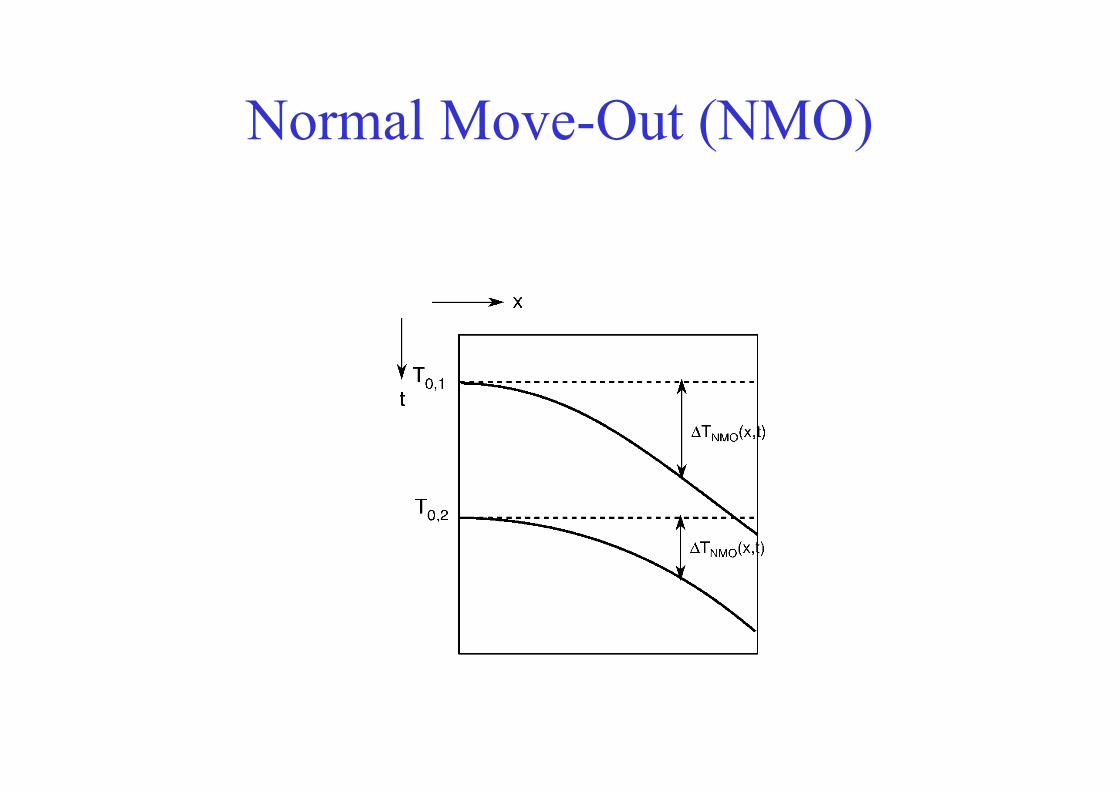
Normal Move-Out (NMO)

Normal Move-Out (NMO)

! TNMO = T - T0 = T0 ( 1 + x2

c2 T02

)1/2 - T0

•  Larger !TNMO for larger offset

•  Smaller !TNMO for larger T0 (deeper layers have smaller move-out)

•  Smaller !TNMO for larger wave speed c (deeper layers usually larger velocities so smaller move-out)

Normal Move-Out (NMO)

Input CMP-gather NMO-corrected CMP gather (with right velocity)

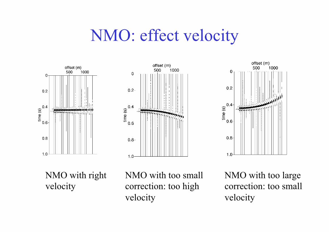
NMO: effect velocity

NMO with right velocity

NMO with too small correction: too high velocity

NMO with too large correction: too small velocity

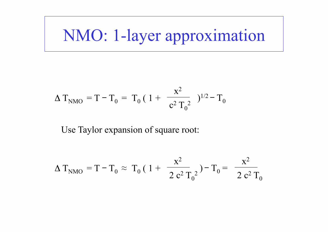
NMO: 1-layer approximation

! TNMO = T - T0 = T0 ( 1 + x2

c2 T02

)1/2 - T0

Use Taylor expansion of square root:

! TNMO = T - T0 ! T0 ( 1 + x2

2 c2 T02 ) - T0 =

x2

2 c2 T0

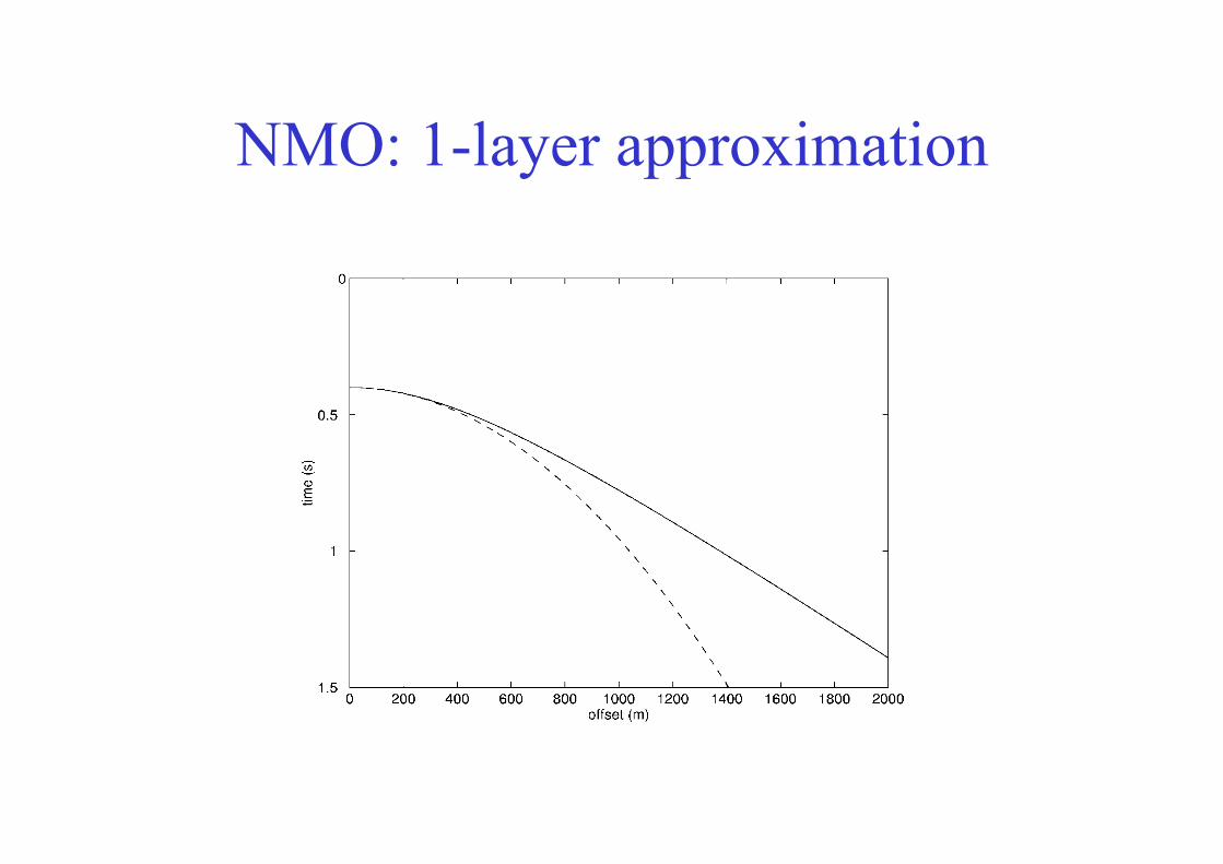
NMO: 1-layer approximation

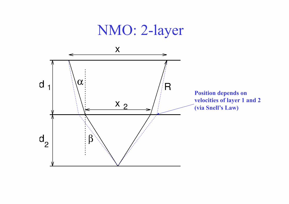
NMO: 2-layer

Position depends on velocities of layer 1 and 2 (via Snell’s Law)

NMO: 2-layer

(pdf-eqs)

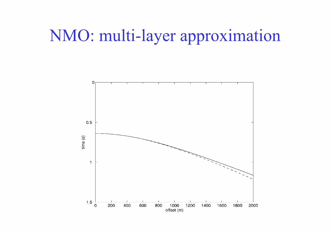
NMO: multi-layer approximation

Velocity model: RMS model

time

velocity

Interval velocity (velocity of layer)

Root-mean-square velocity (weighted-average velocity of layers above)

Velocity Analysis

Approaches: •  T2 – x2 analysis

•  Alignment of reflectors: visually or mathematical expression of coherence

With T2 – X2 analysis we depend on picking travel-times,

and thus signal-to-noise ratio

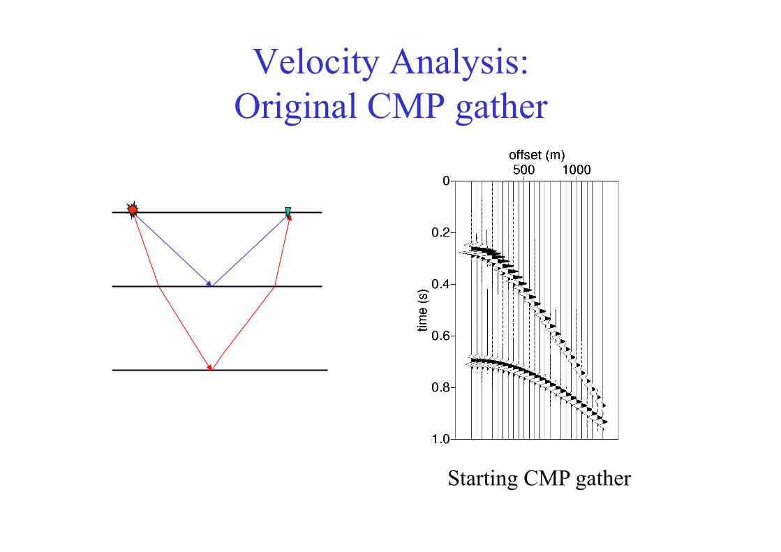
Velocity Analysis: Original CMP gather

Starting CMP gather

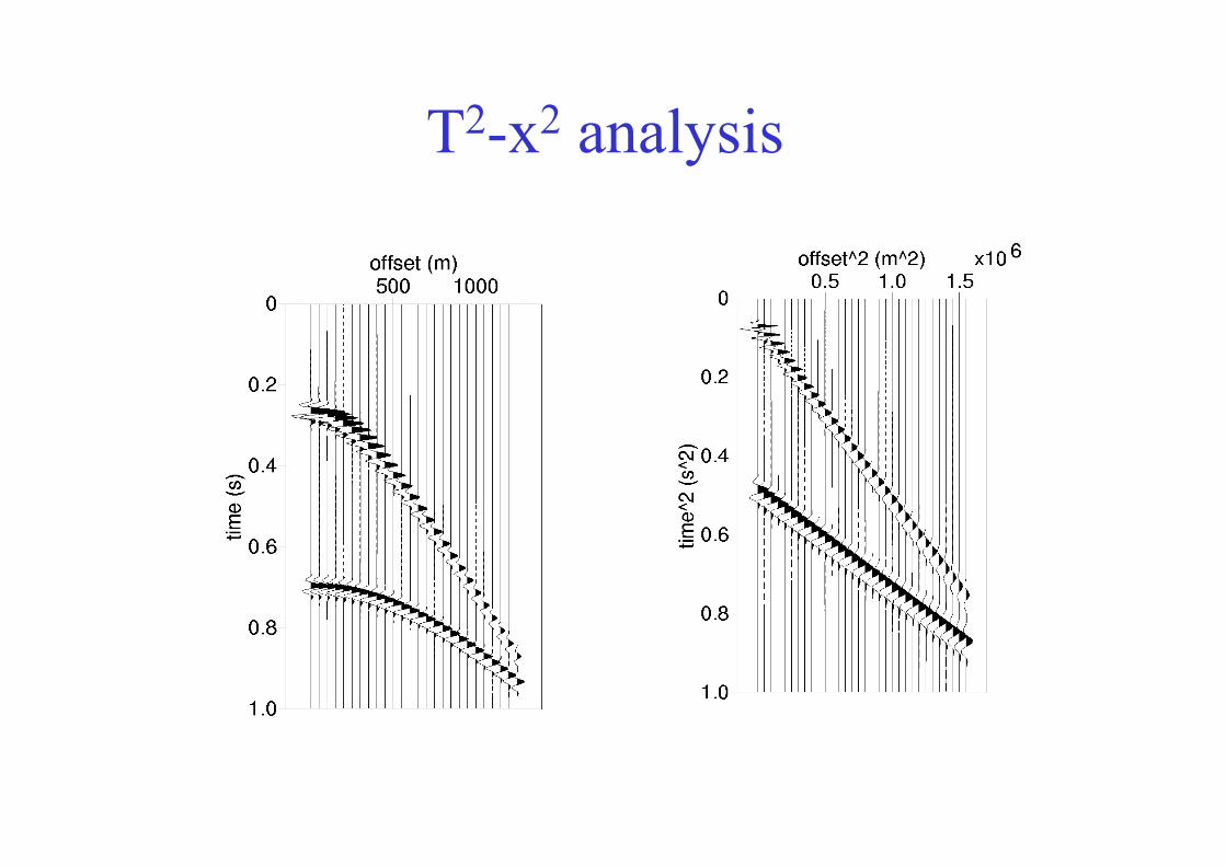
T2-x2 analysis

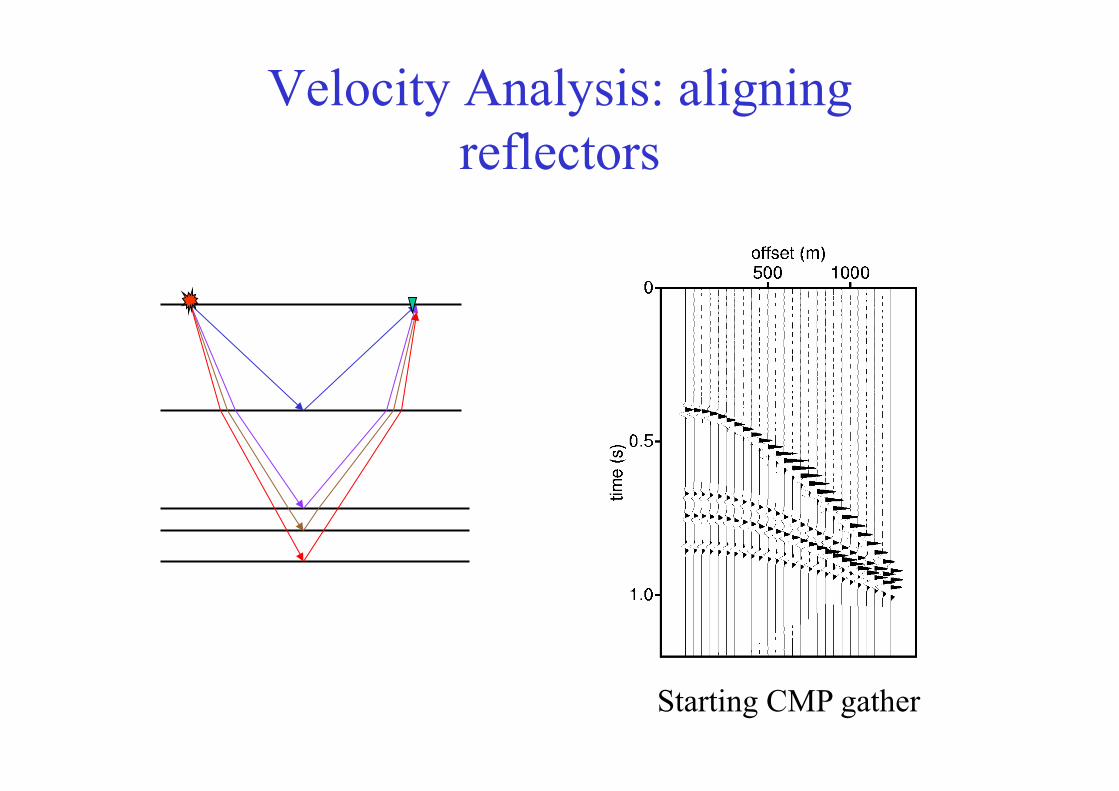
Velocity Analysis: aligning reflectors

Starting CMP gather

Constant-velocity NMO

Velocity too high: correction too little

Velocity too low: correction too much

Velocity panels

CMP gather with velocity

1300 m/s CMP gather with velocity

1700 m/s

CMP gather with velocity

2100 m/s

Velocity as function of time

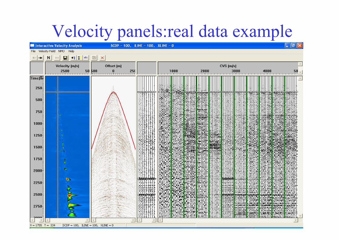
Velocity panels:real data example

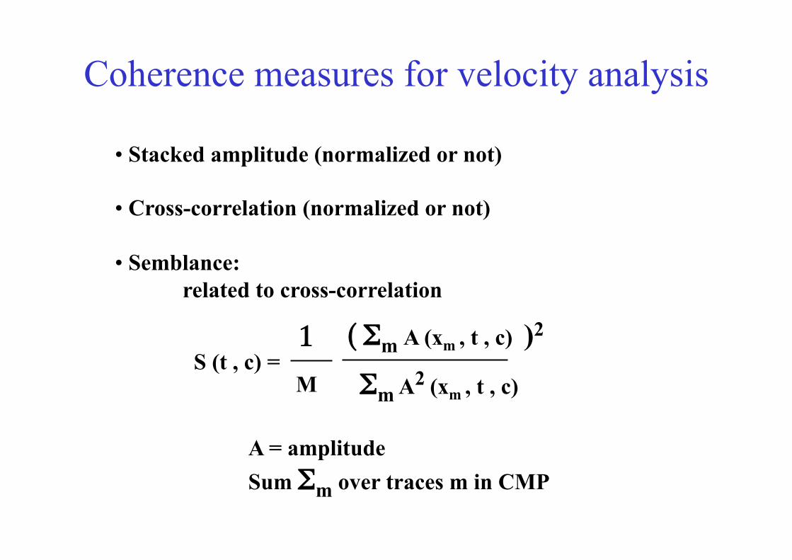
Coherence measures for velocity analysis

•  Stacked amplitude (normalized or not)

•  Cross-correlation (normalized or not)

•  Semblance: related to cross-correlation

A = amplitude Sum "m over traces m in CMP

S (t , c) = ( "m A (xm , t , c) )2

"m A2 (xm , t , c)

1

M

Semblance for CMP gather

Velocity panels:real data example

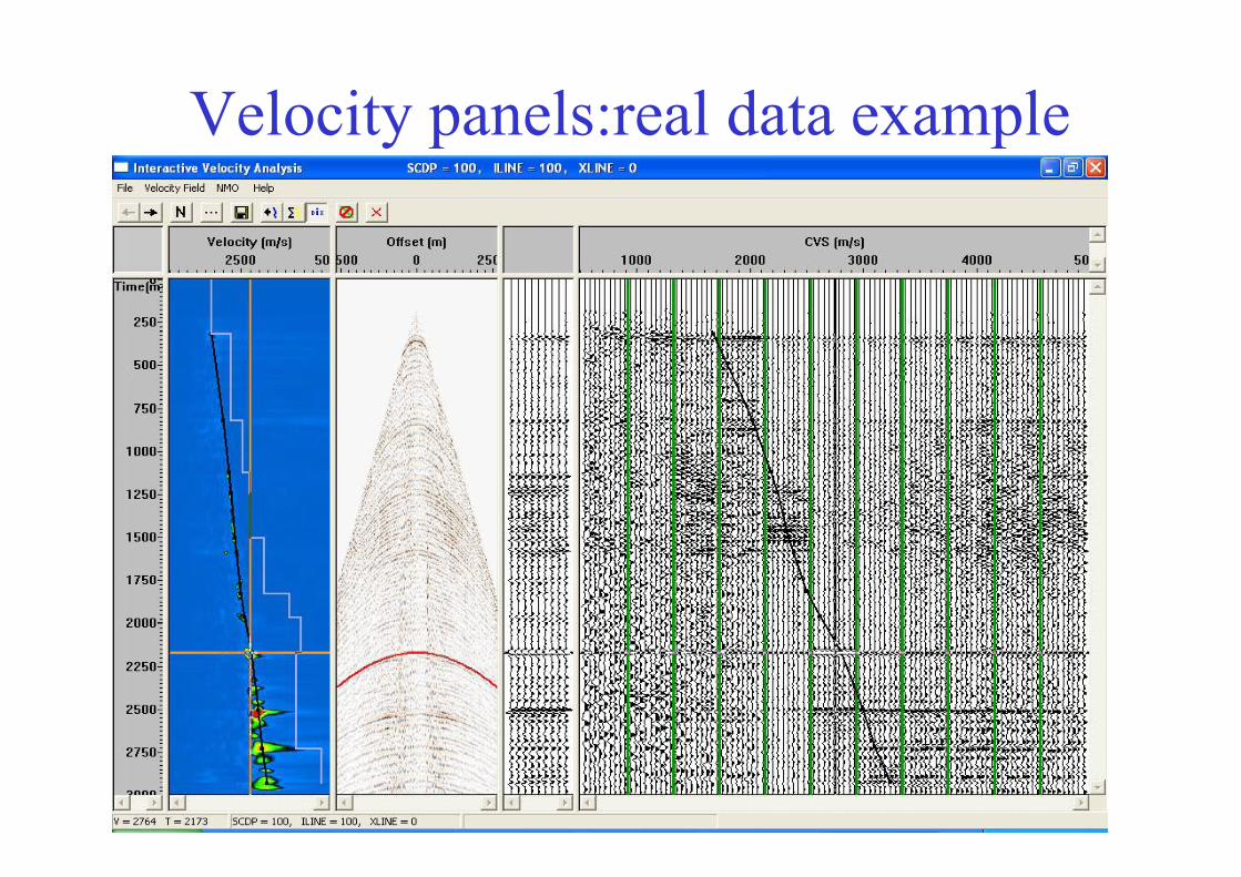
Velocity panels:real data example

Velocity panels:real data example

Factors affecting velocity estimation (Yilmaz, 1988)

•  Spread length

•  Stacking fold / Signal-to-Noise ratio (fold = multiplicity in CMP)

•  Choice of coherence measure

•  Departures from hyperbolic move-out

•  NMO stretch

Effect spread length on velocity estimation

Effect spread length on velocity estimation

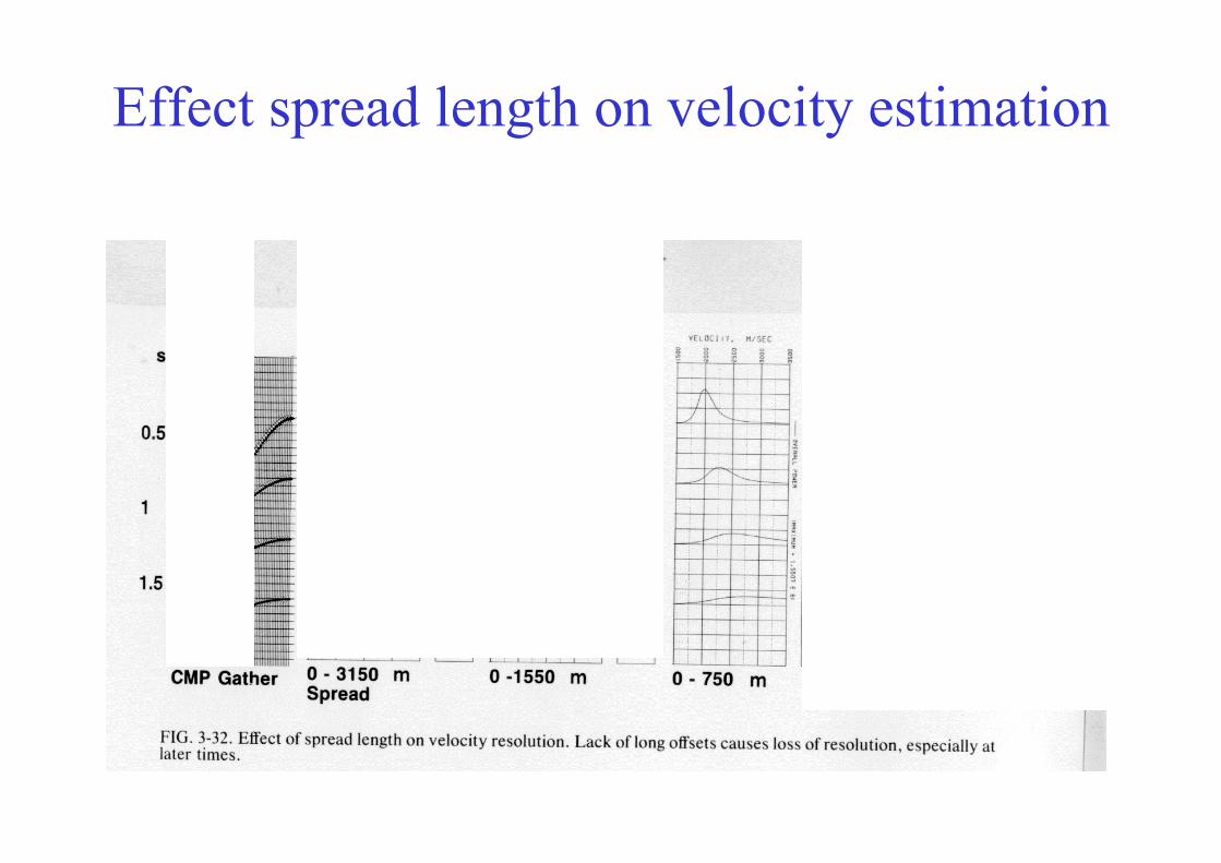
Effect spread length on velocity estimation

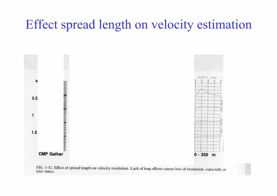
Effect spread length on velocity estimation

Velocity model: RMS model

time

velocity

Interval velocity (velocity of layer)

Root-mean-square velocity (weighted-average velocity of layers above)

Velocity model: RMS model

Time (m

-seconds)

CMP location

CMP sorting

shot data

image

NMO correction

(zero-offset) migration

stack

velocity model

velocity model

Processing flow

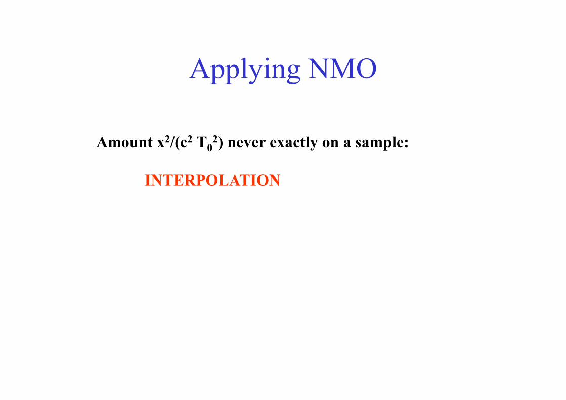
Applying NMO

Amount x2/(c2 T02) never exactly on a sample:

INTERPOLATION

NMO stretch (via picture)

T

T’

Since T0 is larger: shift is smaller

Since T0 is smaller: shift is larger

Hyperbolic shift

NMO stretch (mathematically)

Due to differential working on T as function of T0:

! TNMO = x2

2 c2 T0

" "T0

" "T0

x2

2 c2 T02

= -#

This is called NMO-stretch

NMO stretch

NMO stretch

Amplitude spectra

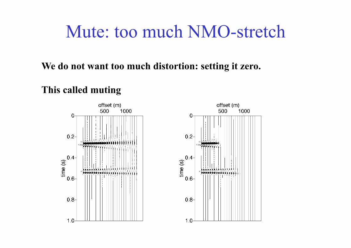
Mute: too much NMO-stretch

We do not want too much distortion: setting it zero. This called muting

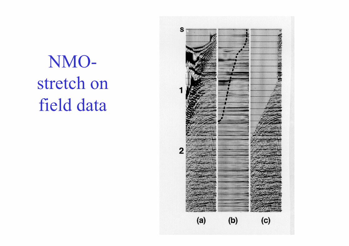
NMO-stretch on field data

CMP sorting

shot data

image

NMO correction

(zero-offset) migration

stack

velocity model

velocity model

Processing flow

Stacking

Add traces from NMO-corrected, CMP gather into ONE trace

Number of traces = stack fold Events that are not hyperbolic, do not add up nicely and

destructively interfere Goal of stacking : to increase signal-to-noise ratio

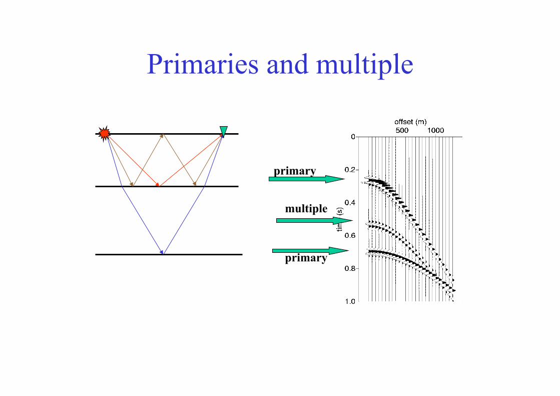
Primaries and multiple

primary

multiple

primary