Preserving Geometry and Topology for Fluid Flowswith Thin Obstacles and Narrow Gaps

Vinicius C. AzevedoInstituto de Informatica - UFRGS

Christopher BattyUniversity of Waterloo

Manuel M. OliveiraInstituto de Informatica - UFRGS

Rotating Paddle: 23× 10× 6 grid Hollow Dragon: 11× 9× 6 grid Linked Tori: 7× 7× 7 grid

Figure 1: Our geometry- and topology-aware boundary treatment supports simulating smooth flows in the presence of thin solid geometry andnarrow gaps on very coarse grids.

Abstract

Fluid animation methods based on Eulerian grids have long strug-gled to resolve flows involving narrow gaps and thin solid features.Past approaches have artificially inflated or voxelized boundaries,although this sacrifices the correct geometry and topology of thefluid domain and prevents flow through narrow regions. We present aboundary-respecting fluid simulator that overcomes these challenges.Our solution is to intersect the solid boundary geometry with thecells of a background regular grid to generate a topologically correct,boundary-conforming cut-cell mesh. We extend both pressure pro-jection and velocity advection to support this enhanced grid structure.For pressure projection, we introduce a general graph-based schemethat properly preserves discrete incompressibility even in thin andtopologically complex flow regions, while nevertheless yieldingsymmetric positive definite linear systems. For advection, we ex-ploit polyhedral interpolation to improve the degree to which theflow conforms to irregular and possibly non-convex cell boundaries,and propose a modified PIC/FLIP advection scheme to eliminatethe need to inaccurately reinitialize invalid cells that are swept overby moving boundaries. The method naturally extends the standardEulerian fluid simulation framework, and while we focus on thinboundaries, our contributions are beneficial for volumetric solids aswell. Our results demonstrate successful one-way fluid-solid cou-pling in the presence of thin objects and narrow flow regions evenon very coarse grids.

Keywords: fluids, coupling, cut-cell, boundaries, thin solids

Concepts: •Computing methodologies→ Physical simulation;

Permission to make digital or hard copies of all or part of this work forpersonal or classroom use is granted without fee provided that copies are notmade or distributed for profit or commercial advantage and that copies bearthis notice and the full citation on the first page. Copyrights for componentsof this work owned by others than the author(s) must be honored. Abstractingwith credit is permitted. To copy otherwise, or republish, to post on serversor to redistribute to lists, requires prior specific permission and/or a fee.Request permissions from permissions@acm.org. c© 2016 Copyright heldby the owner/author(s). Publication rights licensed to ACM.SIGGRAPH ’16 Technical Paper,, July 24-28, 2016, Anaheim, CA,ISBN: 978-1-4503-4279-7/16/07DOI: http://dx.doi.org/10.1145/2897824.2925919

1 Introduction

Compelling fluid animations often result from interactions with mov-ing solid boundaries. However, standard grid-based discretizationsface difficulties when either the boundaries themselves or the spacesbetween the boundaries are thin relative to the grid resolution. Fornarrow flow regions, the challenge is that a typical voxelized viewof the domain simply cannot capture them correctly, either topolog-ically or geometrically. For thin boundaries, the same difficultiesare exacerbated by the need to prevent flow on one side of an im-permeable boundary from erroneously interfering with flow on theopposing side. While in principle one could continually increasethe grid resolution until the thin feature or region is fully resolved,this is tremendously expensive and impractical for most animationscenarios. The poor scaling of volumetric simulation has motivatedrecent efforts to capture as much detail as possible at free surfaceboundaries while using much lower resolution underlying simula-tion grids [Kim et al. 2009; Wojtan et al. 2010; Bojsen-Hansen andWojtan 2013; Edwards and Bridson 2014].

Our goal is philosophically similar: we seek to enhance the abilityof coarse grid-based Eulerian fluid simulators to resolve interestingflows, but focus instead on solid boundaries which may be moving,irregularly shaped, arbitrarily thin, and in close mutual proximity.

We take an embedded boundary or cut-cell approach: at each timestep, grid cells intersected by the triangle mesh representing the solidboundary are clipped against it, potentially yielding multiple distinctpolyhedral sub-cells. The resulting hybrid simulation mesh closelyconforms to the geometry of the solid boundary and reduces to aregular grid away from the boundary. Crucially, and in contrast toexisting fluid animation methods using regular grids, our approachpreserves the topology of the fluid domain, including thin solids andslender narrow gaps between nearby solids. The practical advantagethis offers is a sharp reduction in the unnecessary coupling betweengrid resolution and solid boundary topology present in previouswork; that is, fluid grid resolution can be artistically adjusted solelyto achieve the desired balance of fluid detail and computational cost,without concern for whether an inaccurate solid discretization willinadvertently disconnect or merge flow regions in the process.

We first introduce a topologically-accurate, graph-based discretiza-tion for the pressure projection on the cut-cell mesh which canresolve flows in difficult regions. Furthermore, it offers greaterfidelity than prior work on thin solids: it better accounts for the sub-

grid geometry of the boundary, correctly recovers free-slip boundaryconditions, and is consistent with existing cut-cell approaches forvolumetric objects (e.g., [Batty et al. 2007; Ng et al. 2009]).

Secondly, to improve the handling of advection near boundarieswe develop a conforming velocity interpolant on arbitrarily-shapedpolyhedral cut-cells by relying on spherical barycentric coordinates(SBC) [Langer et al. 2006]. This allows flow characteristics to moreclosely respect boundary geometry than is possible with standard,boundary-oblivious linear or cubic interpolation schemes, particu-larly in narrow regions.

Lastly, we augment our approach with a tailored PIC/FLIP [Zhuand Bridson 2005] advection scheme. Beyond its usual ability toreduce numerical dissipation, this resolves a lingering difficulty withsemi-Lagrangian advection in the context of thin moving boundaries.Specifically, grid cells swept over by solids lack valid velocity infor-mation after semi-Lagrangian advection [Guendelman et al. 2005],and must be filled back in by extrapolating from valid cells that maybe arbitrarily far away. Our use of Lagrangian particles ensures thatvelocity data flows coherently with the boundaries themselves, sothat extrapolation is not required.

These enhancements substantially improve the detail that can beachieved when simulating fluids interacting with solid boundaries,while readily integrating into the dominant Eulerian staggered gridfluid pipeline. Figure 1 shows examples of fluid animations con-taining thin obstacles and gaps created with our technique on verycoarse grids. On the left, a very thin paddle successfully stirs smoke.The image in the center shows smoke propagating through a narrowtunnel in a low-resolution grid. On the right, we see flow throughtwo linked tori without mutual interaction.

To summarize, the technical contributions of our work include:• The identification of key limitations of existing thin solid and

thin gap treatments, due to voxelized geometry and standardinterpolation strategies;

• A symmetric, graph-based cut-cell pressure projection methodthat preserves the domain topology (Section 4). It is the firstto properly handle both thin obstacles and thin gaps betweenobstacles within coarse 3-D grid cells, allowing the use of lesscostly grids to animate flows in difficult geometries;

• An improved velocity interpolation scheme in polyhedral cut-cells based on spherical barycentric coordinates (Section 5),allowing flows to better respect irregular solid boundaries;

• A technique to improve velocity advection near thin movingobstacles (Section 6). By combining Lagrangian PIC/FLIPparticles with our cut-cell scheme, velocity information iscorrectly propagated despite the presence of moving geometry.

1.1 Overview

The structure of our technique is outlined in Algorithm 1, which gen-erally follows the hybrid particle-grid approach of Zhu and Bridson[2005]. After reviewing related work, we describe our cut-cell meshstructure (Section 3) and explain how pressure projection (Section4), interpolation (Section 5) and advection (Section 6) are modifiedto best exploit it. We describe our algorithm in 3-D; the 2-D analogyis straightforward.

2 Previous Work

2.1 Thin Solid Boundaries

While thin boundaries often arise in two-way coupling, we focus ourreview on aspects relevant to the one-way (solid-to-fluid) couplingproblem addressed by our work.

Algorithm 1 Main Loop

while simulating doAdvect particles (Section 5) and advance solid positionGenerate cut-cell mesh (Section 3)Transfer particle velocities to the mesh (Section 6)Add external forces to the meshPerform pressure projection on the mesh (Section 4)Update particle velocities from the mesh (Section 6)

end while

The coupling of fluid to thin boundaries in computer graphics wasfirst addressed by Guendelman et al. [2005]. Their approach vox-elized the geometry of thin shells onto the regular grid, and used aone-sided extension of trilinear interpolation based on raycasting toavoid mixing data from the opposite side of a boundary. They alsoproposed an extrapolation approach to fill in data for fluid regionsthat are swept over and invalidated by moving boundaries. Laterwork by Robinson-Mosher et al. [2008; 2009] adopted essentiallythe same one-sided interpolation mechanism. A similar raycastingstrategy has been applied to compressible flows in computationalfluid dynamics [Wang et al. 2012].

Robinson-Mosher et al. [2008] used a mass-lumping technique fortwo-way coupling of thin shells to fluid on a regular grid. Thisscheme sacrifices free-slip velocities even in the inviscid limit, so thesame authors proposed the use of ghost-velocities and a constraint-based formulation to restrict only the normal component of velocity[Robinson-Mosher et al. 2009]. Both methods use a voxelizedboundary approximation, and thus the topology of the fluid domainused by the pressure solver is often incorrect in tight configurations.Voxelization also leads the solid boundary velocity constraints to beapplied at grid face centres rather than on the actual boundary itself.Qiu et al. [2015] proposed a two-way rigid-body-fluid couplingscheme that extends the voxelized approach to thin gaps using lower-dimensional advection and extra degrees of freedom, though it doesnot consider thin objects.

Boundary-conforming Eulerian tetrahedral meshes (e.g., [Feldmanet al. 2005; Klingner et al. 2006; Elcott et al. 2007]) could potentiallysimplify the treatment of thin boundaries during pressure projection,at the cost of repeated and potentially costly remeshing, but to ourknowledge this has not been explicitly considered. The closest isthe work of Chentanez et al. [2006], who simulated the couplingof fluid to deformable shells of modest thickness discretized withtetrahedra using a conforming mesh approach. To reduce meshingcosts for liquid animation, Chentanez et al. [2007] later relied onthe efficiency of isosurface stuffing [Labelle and Shewchuk 2007];however, isosurface stuffing conforms to an approximate isosurfacerather than the exact solid geometry. In general, while conform-ing meshes simplify the pressure projection, their use in Eulerianschemes does not inherently resolve interpolation and advectionissues near thin boundaries. In contrast to Eulerian methods, purelyLagrangian methods that rely on conforming tetrahedralizations ofboth fluid and solid are also possible [Misztal et al. 2010; Clausenet al. 2013], and may better avoid these issues; again, this does notappear to have been studied.

While beyond the scope of this work, thin objects have also been cou-pled to SPH simulations (e.g., [Lenaerts and Dutre 2008]). Anotherinteresting alternative uses history-based forces to approximate theeffects of fluid on submerged cloth [Ozgen et al. 2010]; this does notextend to scenarios where the fluid motion itself is also of interest.

2.2 Embedded Boundary Methods

Roble et al. [2005] proposed a two-dimensional finite volume-liketechnique for irregular static boundaries, similar to much earlierwork by Purvis and Burkhalter [1979], in which the usual Poissonstencil is augmented with per-face weights that account for the fluidfraction of each face. Batty et al. [2007] presented a closely related,variational technique that enabled stable two-way coupling in 3-Dwith irregular volumetric rigid bodies. Ng et al. [2009] showed thatthe finite volume variant of this scheme yields second-order accuratepressures and first-order velocities. (This complements the ghostfluid method for free surfaces [Enright et al. 2003] which achievesthe same.) In essence, our discretization applies and generalizes thework of Ng et al. to thin boundaries and thin gaps.

Colella and collaborators [Johansen and Colella 1998; Schwartzet al. 2006] developed a similar cut-cell method that additionallyinterpolates velocities to lie at the centroids of partial faces. Thisachieves second-order accurate velocities at the expense of morecomplex stencils; however, these stencils yield non-symmetric sys-tems and cannot be applied in narrow regions. Day et al. presentedan interesting partial extension of this idea to thin boundaries in twodimensions, through the use of a more general graph structure andextra ghost samples on the grid [Day et al. 1998]. Our pressure pro-jection draws inspiration from this method, but differs in a few keyrespects. We achieve a symmetric positive-definite system, providea direct extension to three dimensions, and support an arbitrarynumber of disjoint components per cell.

Crockett et al. [2011] discussed the related idea of “multi-cells”which arise during coarsening steps of a multigrid scheme for Pois-son problems on irregular domains; work by Dick et al. [2016] issimilar in spirit. Weber et al. [2015] developed a multigrid solverfor the scheme of Ng et al., ensuring consistent discretization acrossgrid levels, but did not consider multi-cells or the treatment of thinsolids. Hellrung et al. [2012] presented a more complex virtualnode discretization for 3-D Poisson problems with discontinuities,assuming a level-set description of domain boundaries which effec-tively restricts the method to closed regions that do not possess thinboundaries or gaps.

Ferstl et al. [2014] used a cut-cell tetrahedra-based finite-elementscheme with a multigrid solver, and similarly preserved the freesurface topology during coarsening, though solid boundaries weretreated as voxelized. Edwards et al. [2014] proposed an adaptivediscontinuous Galerkin scheme on cut cell meshes to handle detailedfree surface flow on coarse grids, potentially involving multipledisjoint liquid components per original cell; they did not discuss thinsolids or thin gaps.

Outside of the fluid setting, topology-aware strategies have beenapplied to simulate the dynamics of elastic deformable objects pos-sessing multiple distinct deforming components inside a single finiteelement [Teran et al. 2005; Nesme et al. 2009]. Though conceptuallyrelated, they are inapplicable to the problem we consider.

2.3 Velocity Reconstruction and Interpolation

Staggered-grid projection methods recover only the face-normalcomponents of velocity rather than full vectors; this slightly com-plicates interpolation and advection. In the regular grid case, mul-tilinear interpolation can be applied on each velocity componentindependently. However, for more general unstructured or poly-hedral meshes, full velocities must first be reconstructed beforeinterpolating, typically through least squares fitting, as done by pre-vious work on tetrahedral and Voronoi grids [Feldman et al. 2005;Klingner et al. 2006; Elcott et al. 2007; Sin et al. 2009; Batty et al.2010; Brochu et al. 2010]. We use a least squares fit to recover nodal

velocities from face fluxes on our polyhedral cells, which simplifiesvelocity interpolation during advection.

Various velocity interpolation schemes have been proposed for useduring the advection step, the most common being simple bi/tri-linear interpolation on a regular grid [Stam 1999]. Higher-orderextensions have been used to improve the retention of vorticity[Fedkiw et al. 2001; Selle et al. 2008].

Guendelman et al. [2005] were the first to directly address the inter-polation issues raised by thin boundaries. Subsequent related workby Robinson-Mosher et al. [2008; 2009] relied on the same interpo-lation technique. Raycasting is used to determine visibility betweenan interpolation point and the position of a velocity sample it woulddepend on; one-sided interpolation can then be performed using onlythe visible data to robustly avoid polluting the result with data fromthe opposite side of a thin boundary. However, since basic trilinear ortricubic interpolation do not possess knowledge of the solid position,fluid trajectories typically still cross boundaries; this necessitatesthe frequent use of collision-processing during advection to preventdata crossing over.

On staggered unstructured tetrahedral meshes, the velocity recon-struction approaches are first used to determine velocities at de-sired nodal points; these can then be applied within a mesh-basedbarycentric interpolant. Given the velocities at tetrahedra centres(i.e., Voronoi vertices), generalized barycentric interpolation is ap-plied over the convex Voronoi elements [Klingner et al. 2006; Elcottet al. 2007].

In the above methods, polyhedral interpolants were used for thepurpose of avoiding oversmoothing velocities, as compared to in-terpolating over tetrahedra. By contrast, our primary motivationfor using polyhedral interpolation is that it enables the interpolatedvelocity to closely conform to the geometry of solid boundaries.Rosatti et al. [2005] presented a related two-dimensional techniquethat fits boundary-respecting linear velocity fields to the triangular,trapezoidal, and pentagonal cells resulting from the usual marching-squares cases applied to an implicit representation of the solid bound-ary. Our approach clips the regular grid against the solid boundarytriangle mesh, yielding arbitrary polyhedral cells. We can then usean interpolant that handles non-convex polyhedra, i.e., sphericalbarycentric coordinates [Langer et al. 2006].

3 The Cut-Cell Mesh

Given a triangle mesh representing the geometry of the solid bound-ary, we perform clipping on all cells intersected by this bound-ary. Each affected original grid cell may give rise to one or moreboundary-conforming polyhedral sub-cells. Clipping with trianglemeshes is a well-studied problem (e.g., [Aftosmis et al. 1998; Sifakiset al. 2007; Wang et al. 2014]), most recently used by Edwards andBridson [2014] to support detailed liquid free surfaces. We there-fore refer the reader to these works for implementation details ongenerating cut-cell meshes, and simply summarize the properties ofthe resulting mesh.

A principal difference between our cut-cell meshes and those usedby Edwards and Bridson is that we retain sub-cells on both sides ofthe triangle mesh geometry. The solid geometry is also not requiredto be a “closed” surface, and therefore the triangle mesh may cutonly partway through a cell. In this case, we subdivide the facesthrough which it crosses, but do not partition the cell itself. Wewill refer to the resulting faces as dangling interior faces. We willrefer to mesh faces that connect two fluid (sub-)cells as fluid faces;these will always be axis-aligned. New faces produced by clippingagainst the solid boundary will be called solid faces. We do nottetrahedralize the resulting polyhedra, so cell faces may be general

planar polygons. Cells that are not intersected by the geometry areleft untouched, so as to be efficiently and conveniently treated withstandard methods.

Figure 2 illustrates these cut-cell concepts in 2-D, for two infinites-imally thin solid boundaries with fluid on either side. In (a), thethin boundaries are represented by polylines, shown in green withbright green nodes. The original regular grid is shown in gray. Part(b) illustrates the boundaries (in red) resulting from the raycastingor voxelized view used by previous work [Guendelman et al. 2005;Robinson-Mosher et al. 2008; Robinson-Mosher et al. 2009]. Boththe geometry and topology of the fluid domain are sacrificed: the gapbetween the two solid boundaries has been entirely collapsed away.Part (c) illustrates our cut-cell mesh with the new vertices createdduring clipping (shown in black). Under our cut-cell view, both thethin gap and the detailed geometry of the boundary are maintained.Part (d) uses a graph (blue) to illustrate the neighbour relationshipsbetween the resulting sub-cells. The segments in the partially cutupper-left and lower-left cells are examples of dangling interiorfaces; notice that, as illustrated in the graph view, these partially cutcells are assigned only a single pressure sample although their facesare subdivided.

(a) Geometry (b) Raycast

(c) Cut-cell (d) Graph

Figure 2: (a) Sub-grid thin boundaries (green) are represented by apolyline mesh in 2-D. (b) Voxelization/raycasting yields inaccurateaxis-aligned boundaries (red). (c) Clipping the grid against the solidboundary mesh instead yields a cut-cell mesh with multiple distinctsub-cells, with new mesh nodes shown in black. (d) The connectivityrelationships between sub-cells can be visualized as a graph (blue).

This cut-cell mesh, with its support for multiple disjoint solid compo-nents and multiple sub-cells in each grid cell, forms the infrastructurewith which we will handle narrow gaps and thin solids. An exampleis shown for the Dragon in Figure 3.

4 Graph-Based Pressure Projection

Cut-Cell Pressure Projection The standard pressure projectionstep solves the Poisson problem ∆t

ρ∇ · ∇p = ∇ · u∗, in order to

find the pressure field that will correctly convert the intermediatevelocity field, u∗, into the nearest incompressible field, u. Havingfound the pressure field p, its gradient is subtracted from the velocityfield: u = u∗ − ∆t

ρ∇p.

Our approach to discretizing this problem on the cut-cell meshextends previous variational [Batty et al. 2007] and finite volume cut-

Dragon with Coarse Grid

Intersection Curves

Figure 3: (Top) The dragon solid geometry, shown with the regulargrid superimposed. (Bottom) The network of curves generated byintersecting the two, with the dragon rendered transparent.

cell [Roble et al. 2005; Ng et al. 2009; Batty et al. 2010] techniquesfor volumetric solids, which account for the flow through each faceof a given grid cell adjusted for the area of the faces that are blockedby a solid obstacle.

In particular, we begin with the scheme of Ng et al. [2009] as thebasis of our approach as it yields symmetric positive definite linearsystems and pressure solutions that converge with second-orderspatial accuracy. The associated discrete divergence measure is:

∇ · u ≈∑iAi(u · n)i +

∑j Aj(usolid · nsolid)j

Vcell, (1)

where the index i runs over all fluid faces of a cell, and j runs overall solid faces. Ak indicates the area of the k-th face, u is the fluidvelocity, usolid is the solid velocity, n is the fluid face normal vector,nsolid is the solid face normal vector, and Vcell indicates the volumeof the cell. Face normals are assumed to be oriented outwards.As usual, scaling each row of the discrete Poisson problem by itscorresponding cell volume cancels volume terms in the system;we require only face areas (e.g., [Losasso et al. 2004]). FollowingGuendelman et al. [2005] one must also take care to set the velocityfor the solid boundary condition to be the effective velocity computedover the subsequent timestep rather than its instantaneous/analyticalvelocity, to ensure that the resulting end-of-step velocities sync withthe motion of the solid during advection on the next step; their paperprovides further discussion.

Pressure gradients are computed using standard centered differencesbetween cell-centered pressures, ∇p ≈ pi+1−pi

∆x, even near cut-

cell faces. Given these discrete divergence and gradient operators,the Poisson problem can be directly discretized on the usual stag-gered grid. Perhaps surprisingly, Ng et al. clearly show that thisprojection scheme correctly converges even though the geometriccenters of cells and the midpoints of faces often lie outside the ac-tual fluid domain (see Figure 4, top-left). This feature conveniently

preserves many of the benefits of the structured regular grid (symme-try, positive-definiteness, primal-dual orthogonality, second-orderaccurate pressures) as we extend it to more general topologies below.

Figure 4: Top-left: The method of Ng et al. for embedded volumetricsolid boundaries (green) converges despite using active face mid-points (black dash) and cell centers (black disks) lying outside thefluid domain (white). Top-right: A complementary dual geometry,created by swapping fluid and solid domains, can also be easilysimulated with Ng’s method. Bottom-left: By conceptually superim-posing the top two scenarios and duplicating the required degreesof freedom, a pressure projection can be performed on the thin solid,shown at the bottom-right, without interference across it.

Topology-Aware Pressure Projection The method of Ng et al.implies a few restrictions. It assumes a level set description of the ge-ometry, which limits it to volumetric objects and fluid regions largerthan a grid cell width to guarantee a faithful topological descrip-tion of the domain. The strictly regular underlying grid structurealso means that each cell contains only a single active region andcorresponding pressure . We seek to relieve these restrictions.

To extend this strategy to multiple distinct flow regions within a sin-gle regular grid cell, as produced by our mesh clipping strategy, wetake inspiration from recent virtual node [Molino et al. 2004; Hell-rung et al. 2012] and topology-preserving [Teran et al. 2005; Nesmeet al. 2009] schemes. We allow multiple disjoint active sub-cellswithin a single original cell, with additional pressure and velocitydegrees of freedom that conceptually coincide for consistency withNg’s discretization (see Figure 4). We assign one pressure to eachsub-cell, placing it at the original cell center’s location (i.e., not atsub-cell centroids). Each original fluid face of the grid has multiplefluid sub-faces which connect sub-cells of adjacent regular cellstogether; each sub-face is assigned a velocity degree of freedom thatis geometrically positioned at the regular cell face midpoint (i.e., notat the sub-face midpoint). This yields a more general graph structure(see Figure 2d) on which we can perform the pressure projection,yet the gradient and divergence operators remain axis-aligned. Ta-ble 1 gives the explicit matrix representation of our discrete Poissonequation for the small 2-D scenario shown in Figure 5. In largeexamples, most of the mesh will exhibit the usual banded Poissonmatrix structure, with a few additional unstructured entries to treatregions involving cut geometry.

Primal-Dual Orthogonality As highlighted by Batty et al. [2010],orthogonality of the discrete gradient estimates with respect to theface-normal velocity components is key to preserving accuracy instaggered finite volume approaches. For example, staggered octreeschemes [Losasso et al. 2004] can lose accuracy at T-junctions dueto non-orthogonal gradients between large and small neighbor cells,without a more careful treatment [Losasso et al. 2005]. By contrast,the gradients we use between sub-cells are always computed be-tween the geometric centers of their original grid cells, and thereforepreserve orthogonality with respect to the grid faces (see Figure 6).This property is key to both our method and that of Ng et al.

c1,1

sc1 sc5

f1-2

f1-3

sc6

c2,1

sc4sc2f2-4 f5-6

sc7f4-7

sc3f3-5

Figure 5: Geometry and notation used in our 2-D Poisson matrixexample (Table 1). The solid thin boundary is shown in green. ci,jis a regular grid cell at row j, column i. sck is sub-cell k. fa-b isthe fraction of the fluid edge shared by sub-cells a and b.

Figure 6: Left: Naıve octree discretizations yield face fluxes (blue)and pressure gradients (red) that are not aligned. Right: FollowingNg, our cut-cell discretization co-locates all sub-cell pressures atgrid cell centers (filled black circle) rather than sub-cell centroids(empty black circles). Thus our “T-junction-like” branching pre-serves orthogonality and avoids artifacts. Similarly, face fluxes areconceptually stored at original face midpoints (blue), rather than atsub-face midpoints.

5 Conforming Interpolation on Cut-Cells

Both PIC/FLIP and semi-Lagrangian advection schemes rely onthe ability to interpolate velocities at arbitrary points in the fluiddomain. The interpolants used to estimate pointwise velocity valuesin grid-based methods typically rely on simple piecewise linear orcubic approximations [Fedkiw et al. 2001]. Though effective in freeflowing regions, such interpolants are fundamentally oblivious to thedomain geometry, regardless of either the order of the interpolant orthe accuracy of the pressure projection. As a result, the interpolatedfluid velocities do not necessarily satisfy the desired no-penetrationboundary condition ufluid · n = usolid · n, but are instead oftendirected towards and through the boundary, a fact which is particu-larly problematic for thin solids. The most common treatment is toapply collision detection to directly clip particle trajectories againstsolids (e.g., [Fedkiw et al. 2001; Guendelman et al. 2005]), althoughthis can exacerbate artificial clumping of particles and other data[Rasmussen et al. 2004].

We instead aim to construct an improved interpolant so that the fluidvelocities themselves better respect the solid geometry, and relianceon explicit collision-processing can be reduced. Figure 7 uses astreamline visualization to compare one-sided bilinear interpolation[Guendelman et al. 2005; Robinson-Mosher et al. 2009] against ourinterpolation method. Although both approaches carefully avoidmixing data from the wrong side of the thin boundary, the latteryields a velocity field that conforms more closely to the boundary,reduces grid-dependence, and can easily be set to satisfy either afree-slip or no-slip condition as desired. By contrast, the results forbilinear interpolation do not align with the boundary and exhibitnearly identical results under free-slip and no-slip conditions.

We describe our interpolation approach below, and use it during the

c1,1 c2,1 sc1 sc2 sc3 sc4 sc5 sc6 sc7

c1,1 2 −1 −1 0 0 0 0 0 0c2,1 −1 3 0 −1 0 0 0 0 −1sc1 −1 0

∑f1 −f1-2 −f1-3 0 0 0 0

sc2 0 −1 −f1-2∑

f2 0 −f2-4 0 0 0sc3 0 0 −f1-3 0

∑f3 0 −f3-5 0 0

sc4 0 0 0 −f2-4 0∑

f4 0 0 −f4-7sc5 0 0 0 0 −f3-5 0

∑f5 −f5-6 0

sc6 0 0 0 0 0 0 −f5-6∑

f6 0sc7 0 −1 0 0 0 −f4-7 0 0

∑f7

p1,1

p2,1

psc1psc2psc3psc4psc5psc6psc7

=

d1,1

d2,1

dsc1dsc2dsc3dsc4dsc5dsc6dsc7

Table 1: The symmetric cut-cell pressure projection matrix that results from the 2-D configuration shown in Figure 5, assuming Neumannboundary conditions on the domain perimeter. ci,j represents a regular grid cell at row j, column i. sck is sub-cell k. fa-b is the fraction of thefluid edge shared by sub-cells a and b.

∑fk is the sum of all fluid-edge fractions shared by sub-cell sck. pi,j and di,j are, respectively, the

pressure and divergence at grid cell ci,j . psck and dsck are the pressure and divergence at sub-cell sck.

(a) SBC (free-slip) (b) SBC (no-slip)

(c) Bilinear (free-slip) (d) Bilinear (no-slip)

Figure 7: Streamlines of a velocity field obtained using differentone-sided interpolation schemes, with a stationary flow on one side.(a) SBC interpolation from nodal velocities using free-slip bound-ary conditions leads to streamlines that flow smoothly along theboundary. (b) SBC with no-slip likewise conforms to the boundary,but both tangential and normal velocities drop to zero precisely atthe boundary. (c) and (d) show one-sided bilinear interpolationfrom values stored at the regular grid corners for both free-slip andno-slip. The bilinear results exhibit grid-dependence, and do notdiffer appreciably from one another. Moreover, since the interpolantis non-conforming, the relevant velocity components do not drop tozero on the boundary curve.

particle advection step of Section 6.

5.1 Polyhedral Cut-Cell Interpolation

Away from solid boundaries, we apply standard trilinear interpola-tion to the regular grid velocities. For polyhedral (sub-)cells abuttingthe solid geometry, we will first reconstruct nodal velocity values(Section 5.2), and use these values for interpolation.

To perform interpolation over potentially non-convex polyhedra withgeneral planar polygonal faces, we make use of spherical barycentriccoordinates (SBC) [Langer et al. 2006], which provide a convenientgeneralization of standard barycentric coordinates to this case. Weselect SBC over the more widely-known mean value coordinates [Juet al. 2005], because SBC supports polygonal rather than triangularfaces. This method is effective for the vast majority of cut cells, andthe result is a nicely conforming interpolant.

Unfortunately, SBC cannot be readily applied to the comparativelysmall set of cells containing dangling interior faces, as this representsa degenerate configuration (essentially two coincident but oppositelyoriented faces). The simplest way to treat this is to just thicken orextrude the input geometry into a very slim volume before simulat-ing. This naturally eliminates problematic dangling interior faces,allowing SBC to work as usual. However, while the geometry is thinit is no longer of infinitesimal width.

The alternative is to try to construct an interpolant that is effec-tive in the presence of the problematic dangling faces. We exper-imented with various approaches, including visibility-aware SPHinterpolation, visibility-aware Shepard [1968] (i.e., inverse distance-weighting with a raycast check of mutual visibility) interpolation,or simply ignoring the dangling geometry altogether and revertingto trilinear interpolation similar to previous work. None of thesechoices is entirely satisfactory, because none ensure a velocity fieldthat is consistent with interpolation on neighbouring cells, conformsto the interior geometry, and avoids mixing data from opposing sidesof the geometry. For examples involving truly infinitesimal widthgeometry, we used the Shepard interpolation approach; we highlightthis as an interesting challenge for future work.

5.2 Velocity Reconstruction

Free-Slip Case We distinguish two cases for reconstructing nodalvelocities on cut-cells: free-slip and no-slip. We consider free-slipfirst, in which the solid velocity determines the normal component,and fluid velocities must dictate tangential components.

We define three types of cut-cell nodes, illus-trated to the right. Fluid nodes (cyan) are theoriginal nodes of the regular grid outside theobject, for which all incident faces are axis-aligned fluid faces. Solid nodes (black) arenodes on the solid for which all incident facesare solid faces. Finally, mixed nodes (white)are nodes incident on both solid and fluid faces generated by the

clipping process. Recovering a full velocity at fluid nodes is triviallydone by averaging from the staggered data on the incident fluidfaces.

For mixed nodes, we apply a weighted least squares fit to the normalvelocity components corresponding to the incident faces (solid andfluid) on the same side of the solid boundary, similar to previouswork [Feldman et al. 2005]. We use the (inverse) distances from thenode to the face centre as the weights. The system can occasionallybe underdetermined if a mixed node has nearly co-planar faces;however, this can be compensated for by incorporating extra face-normal velocity samples from additional nearby faces.

If all of a node’s incident faces are solid faces, we extrapolate fromthe nearby mixed nodes for which a valid velocity has been recon-structed as described above; let us call these valid nodes. We callinvalid nodes the solids nodes for which we have yet to assign avelocity. In 2-D, we perform this extrapolation by simply linearinterpolating along the solid boundary curve inside the cell.

In 3-D, the geometry is a set of surface triangles ratherthan a piecewise linear curve, and we still have solid nodes(black) and fluid nodes (cyan). However, we also distin-guish two types of mixed nodes: edge-mixed nodes (white),which lie on edges of the original grid, and face-mixednodes (magenta), which lie on faces of the original grid.Starting from reconstructed velocity data atedge-mixed nodes, we linearly interpolatealong the solid boundary curves so that everyface-mixed node on the boundary curve hasvalid data. We label the internal (solid) nodesof this surface patch to be initially invalid, andperform a simple iterative averaging approachto extrapolate into the interior solid geometry:all invalid nodes with a valid neighbour areset to the average of the valid neighbours, and then marked as valid.This process is iterated until no invalid nodes are left. Once allinterior nodes have valid data assigned, we perform a few additionaliterations of repeated averaging to smooth the velocities towards asteady distribution. To avoid the damping of velocities introduced bythis averaging process, we perform this step for vector magnitudesand directions separately, re-combining them at the end.

We further improve the degree to which the interpolated velocityremains tangent to the solid by directly projecting out the normalcomponent of the relative velocity between the solid and the fluidfor mixed and solid nodes (similar in spirit to constrained velocityextrapolation [Houston et al. 2003; Rasmussen et al. 2004]). Thisamounts to computing a new fluid velocity as

u′fluid = ufluid − ((ufluid − usolid) · nsolid)nsolid. (2)

We observe that even if nodal velocities are projected to be orthogo-nal to vertex normals, the interpolated flow may still clearly crossboundaries if the geometry is sharply concave. In 2-D, we furtherhandled this by treating sharp corners with a no-slip condition, andsmooth curves with the preceding approach; this can be observed inour results. However, in 3-D such a treatment is not straightforward,and we have not pursued it.

We do not reconstruct full velocities at face-mixed nodes, as theymay lack enough data to reconstruct a full 3-D fluid velocity. How-ever, there are cases where a boundary loop consists of only face-mixed nodes, and no edge-mixed nodes, e.g. a cylindrical tube withdiameter less than a grid cell width cutting horizontally through acell face. The face-mixed nodes on the boundary of the cylinderhave only one fluid face component, and the solid normal contribu-tion may only reliably determine one of the remaining two axes. At

present, we are therefore limited to scenarios in which each sucha solid geometry patch includes at least one edge-mixed node onits boundary. (A reasonable approach in severely under-resolvedcases would be to reconstruct the available dimensions, and set thethe remaining dimension to zero. In the cylindrical example, themissing dimension would correspond to circular rotations aroundthe cylinder’s dominant axis, which is not provided by the fluxesalong the axis or the solid normal velocities perpendicular to it.)

No-Slip Case If no-slip interpolation is preferred for visual pur-poses, fluid nodes are again treated using least squares, but all mixedand solid nodes are directly assigned the solid velocity, including itstangential component. However, note that no-slip conditions willtend to rapidly damp out relative tangential flow in very slender gaps.This is because fluid nodes are the only nodes that no-slip conditionsdo not effect, and narrow gaps may contain relatively few such nodes.Hence, velocities in these sub-cells will be totally dominated by thesolid, and will halt the flow entirely near static solids; an examplecan be seen in Figure 10(d). (No-slip can also lead to extra particleclumping, because it is fundamentally inconsistent with the inviscidfree-slip condition inherent in the pressure solve.)

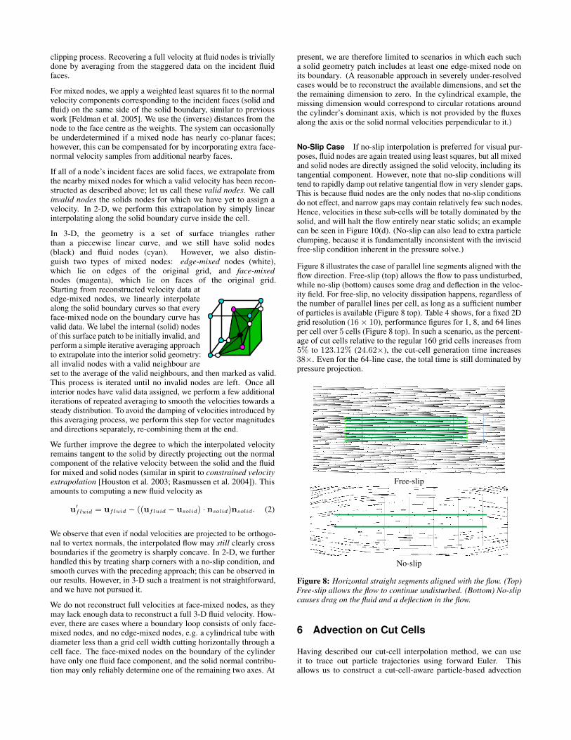
Figure 8 illustrates the case of parallel line segments aligned with theflow direction. Free-slip (top) allows the flow to pass undisturbed,while no-slip (bottom) causes some drag and deflection in the veloc-ity field. For free-slip, no velocity dissipation happens, regardless ofthe number of parallel lines per cell, as long as a sufficient numberof particles is available (Figure 8 top). Table 4 shows, for a fixed 2Dgrid resolution (16× 10), performance figures for 1, 8, and 64 linesper cell over 5 cells (Figure 8 top). In such a scenario, as the percent-age of cut cells relative to the regular 160 grid cells increases from5% to 123.12% (24.62×), the cut-cell generation time increases38×. Even for the 64-line case, the total time is still dominated bypressure projection.

Free-slip

No-slip

Figure 8: Horizontal straight segments aligned with the flow. (Top)Free-slip allows the flow to continue undisturbed. (Bottom) No-slipcauses drag on the fluid and a deflection in the flow.

6 Advection on Cut Cells

Having described our cut-cell interpolation method, we can useit to trace out particle trajectories using forward Euler. Thisallows us to construct a cut-cell-aware particle-based advection

scheme that addresses an issue faced by previous Eulerian andsemi-Lagrangian schemes in the presence of moving boundaries.Specifically, solid boundaries thatsweep over the stationary Euleriangrid leave behind cells lacking ve-locity data. Consider the inset ex-ample: a volumetric circular solid(green) translates past to reveal theformerly inactive central cell (light blue). It suddenly becomes ac-tive again and its faces must be assigned valid velocity data beforecontinuing the simulation. Mittal and Iaccarino [2005] dub these“freshly-cleared” cells. While physically, fluid velocities would sim-ply advect along with the object and fill in the missing data, thisis not true in the discrete case for Eulerian and semi-Lagrangianschemes.

For large volumetric solids, semi-Lagrangian advection suffices,since the velocities previously extrapolated into the solid are oftenreasonable. However, for relatively thin boundaries, (sub-)cell re-gions often go from one side of a moving solid boundary to anotherin a single step, and there is no extrapolated velocity already present“inside” the object. Using semi-Lagrangian advection, the end-of-trajectory velocity value which one would ordinarily use to beginbacktracing from lies on the wrong side of the boundary, where thefluid may be flowing in entirely the wrong direction.

Guendelman et al. [2005] observe this issue, and instead reinitializethese cells by using an iterative averaging procedure to extrapolatedata from nearby fluid cells on the same side which were not sweptover, and hence contain valid data. However, this choice has twoshortcomings illustrated in (Figure 9): in the case of closed invalidregions, data must be created from scratch, or it may result in databeing extrapolated quite long distances (e.g., in narrow regions).

valid

invalid validvalid invalid

Figure 9: Failure cases for standard velocity extrapolation fromvalid into invalid (uninitialized) cells. Left: Closed regions cannotbe extrapolated into. Right: Long narrow regions may requireextrapolation across arbitrary distances.

We observe that with an appropriate PIC/FLIP implementation, thisissue does not arise. Given a sufficient sampling of Lagrangianparticles, there is no need for backtracing or extrapolation; velocitydata carried by the particles travels forwards in tandem with the solidboundary to fill the freshly cleared cells, much like in the physicalworld. We maintain a good sampling of particles throughout byplacing a user-defined lower and upper bound on the number ofparticles per unit area, and reseeding on each sub-cell independently.To complete our advection scheme, we just need mechanisms totransfer particle velocity data to and from the cut-cell mesh.

Transfer to Mesh We transfer velocity information carried bythe particles onto the simulation mesh nodes by setting each nodalvelocity to be a weighted average of the velocity of all particles inthe cells incident on that node. We use SPH kernels throughout, withone minor twist in presence of solid geometry. We use a raycast tocheck whether the node in question is visible from the particle, andif not, we discard its contribution to that node. When face-normalvelocity components are needed by the pressure solve, they arecomputed by interpolating the velocity vector from the cell nodes

and taking the dot-product with the corresponding face normal. Weuse an SPH kernel radius of twice the grid cell width, although onecan safely use smaller kernels provided they cover one full cell.

Transfer to Particles Interpolation of data from the simulationmesh back to the particles is performed using our enhanced inter-polation scheme. This allows for a standard PIC or FLIP update tobe performed. We found that using FLIP in cut cells leads to insta-bility, particularly for small cells; we conjecture that the inherentinstabilities in the FLIP scheme are exacerbated in the presence ofsuch small cells. Therefore, we revert to a pure PIC approach in cutcells, using FLIP only in the broader domain.

As we discuss later in Section 8, truly ideal boundary-respectingtrajectories are infeasible with discrete time-integrators due to nu-merical error; however, for the remaining particle trajectories thatdo cross the boundary, it is necessary to rely on direct collision de-tection and response as in previous work [Guendelman et al. 2005].Nevertheless, because of our conforming velocity fields, the majorityof particles do not cross over or collide.

7 Results

We refer the reader to our supplemental video for various results inboth 2-D and 3-D, which we summarize below. Timings and settingsare given in Table 2; all our results are computed using a single coreof an Intel i7-2600 CPU at 3.4 GHz with 8GB memory. The robustintersection processing needed for mesh generation is handled withthe CGAL library [CGAL 2016]. We simulated a single timestepper frame.

While we focus primarily on coarse grids, Table 3 shows how ourtechnique scales with increasing grid resolution. It provides somecut-cell statistics and performance numbers for a fluid flow around aBunny model (5,002 triangles) with grid resolutions ranging from83 up to 2563. Timings were obtained by averaging five measure-ments with identical settings. As expected, as the number of regularcubic cells increases by a factor of 23 from one grid resolution tothe next, the number of cut cells only increases by a factor of 22.Consequently, the percentage of cut cells (relative to the numberof grid cells) reduces by a factor of 2; that is, for any given solidgeometry, the relative overhead associated with handling irregularcells decreases as grid resolution increases. The cut-cell generationtime is dominated by CGAL operations (ranging from 80% to 90%of the time for resolutions up to 1283). The identification of all faces(both mesh and grid ones) incident to each mixed node is currentlyperformed in a brute force and unoptimized fashion, and thus its cost(column Mixed Nodes in Table 3) increases by a factor of roughly15 from one resolution to the next; this rapid growth ultimatelycauses it to reduce CGAL’s relative contribution to the overall timeat the 2563 grid level. We expect that optimizing this procedure willsignificantly accelerate cut-cell generation at high resolutions. Therightmost columns of Table 3 show the advection and projectiontimes involved in simulating a single time step.

Our simulations do not apply vorticity confinement or other artificialturbulence-creation mechanisms, although these could be easilyadded. Our 3-D examples use 64 or 128 PIC/FLIP particles percell, while our 2-D examples use 32 or 64 particles; these counts arehigher than normal because we want to ensure that even small orskinny cells are sufficiently well-sampled. A smart adaptive particlesampling scheme would likely bring these values down with minimalimpact on the results.

Example Advection Time Projection Time Total Time Meshing Grid Dims No. Cut-CellsLinked Tori - Free Slip 0.372 0.040 0.597 0.443 (once) 7× 7× 7 88Bunny - No Slip 0.343 0.004 0.516 1.527 (once) 7× 7× 7 78Bunny - Free Slip 0.490 0.004 0.881 1.469 (once) 7× 7× 7 78Dragon (fine) - Free Slip 1.124 0.301 2.686 7.984 (once) 19× 14× 11 1298Dragon (coarse) - Free Slip 0.880 0.172 1.986 4.446 (once) 11× 9× 6 326Disk - Free Slip 0.319 0.118 0.63 0.197 (per frame) 25× 21× 13 137Disk - No Slip 0.296 0.105 0.554 0.200 (per frame) 25× 21× 13 137Rotating Paddle - No Slip 0.290 0.148 0.597 0.153 (per frame) 23× 10× 6 67

Table 2: Timing and parameters for 3-D simulations. Timing information is in seconds per frame, and is computed as an average over thefirst 3-4 frames. Total time excludes meshing, listed separately. For moving geometry, the cut-cell count is given for the first frame. For staticmeshes, meshing occurs only once at the start. All examples use 64 particles per cell, except the Linked Tori with 128.

CC Generat. CGAL CGAL Mixed Advect ProjectGrid Resolution # Cut-Cells % Cut-Cells # Polygons Time (sec) (sec) (%) Nodes (sec) (sec) (sec)

8× 8× 8 90 17.58 7,810 0.82 0.68 82.06 0.0004 0.54 0.00616× 16× 16 316 7.71 10,636 1.31 1.15 87.95 0.0012 0.71 0.04532× 32× 32 1,359 4.15 17,502 2.81 2.55 90.43 0.0168 1.24 0.95664× 64× 64 5,260 2.01 32,342 7.85 6.62 84.36 0.2030 2.57 10.094

128× 128× 128 20,943 1.00 70,034 29.20 23.37 80.06 3.0822 7.80 47.218256× 256× 256 83,518 0.50 176,584 172.33 111.12 64.48 49.0320 17.09 224.981

Table 3: Statistics for a fluid simulation around the Bunny model (5,002 triangles) on grids of various resolutions. For each grid resolution,the table provides the number of cut cells (# Cut-Cells), its percentage with respect to the total number of cubic cells in the regular grid (%Cut-Cells), the number of triangles in the Bunny mesh after intersecting with the grid (# Polygons), the total time in seconds required togenerate the cut cells (CC Generat. Time), the subset of the cut-cell generation time spent on CGAL operations (CGAL (sec)), the percentage ofthe cut-cell generation time corresponding to CGAL operations (CGAL (%)), the time spent by our meshing algorithm in the key step of findingall faces incident on each mixed node (Mixed Nodes), and the advection and projection times for simulating one time step.

7.1 Flow through narrow regions

Branching Tube Figure 10 shows a challenging example of flowin a thin gap: a narrow tube, whose width is less than that of agrid cell, turns and branches, creating numerous cut cells and a richtopology. This illustrates the ability of our technique to handle flowsthrough complex regions defined by closely spaced thin boundaries.Results are shown for interpolation using both free-slip (top) andno-slip (bottom) rules. Here and elsewhere free-slip is generallypreferred for its superior behavior, but we show various exampleswith no-slip for completeness.

Ghost in Maze A similar but more elaborate example in 2-Dfeatures a complex maze structure, with a “ghost” character travelingthrough. Again the fluid follows the solid geometry well on thecoarse grid.

Dragon and Linked Tori The teaser (Figure 1, middle and right)shows two 3-D examples of flow through quite narrow regionsdiscretized with few cells: a passage through the dragon mesh (griddimensions: 11 × 9 × 6), and two linked tori (grid dimensions:7× 7× 7). The forcing is provided by setting a velocity boundarycondition on a few faces at one end of the thin region. We rana second version of the dragon at approximately twice the gridresolution in each dimension; while the flow is indeed smootherat finer resolution, it flows in essentially the same fashion as itsless well-resolved counterpart. It is this tradeoff of quality and cost,independent of the geometry, that we seek to provide the user.

7.2 Flow around irregular objects

Three Circles We demonstrate that our method is also effective forstandard solid volumetric objects in close proximity by simulatingflow through thin gaps between a set of three circles in 2-D.

Bunny Figure 11 illustrates the improved quality of flow aroundcoarse 3-D objects (5,002 triangles) as well. Conforming polyhedral

interpolation ensures a reasonable motion that follows the curves ofthe bunny even on a 7× 7× 7 grid. Trading computational cost forquality, Figure 12 shows how the level of turbulent detail increaseswith higher resolution grids.

7.3 Flow around thin objects

Oscillating Lines A sequence of examples in our video featuretwo vertical line segments oscillating back and forth horizontally. Atthe closest point of their trajectories, the segments occupy the samecolumn of grid cells, dividing them into three sub-cells; even in thisextreme case the flow behaves naturally. We can see all our contribu-tions in action: the cut-cell pressure projection yields proper fluxes,our PIC/FLIP particles ensure coherent motion without velocity ex-trapolation for swept-over regions, and our modified interpolationyields particle motion that conforms closely to segments. A close-upillustrates that with free-slip interpolation, the fluid flows verticallyeven as it is squeezed out of the slender sub-cell narrow gap at theclosest position. With no-slip, the interpolated vertical velocities inthe gap drop to zero when the segments enter the same grid column,since they are forced to match that the solid.

Diagonal Line We further illustrate the accuracy of the ideal free-slip conditions with a 2-D example of a diagonal solid line embeddedin a perfectly tangential flow, showing that it does not disrupt theflow unless it rotates.

Stirring Line To test free-slip in a related scenario where theobject is moving and the flow is stationary, our video includes a 2-Dexample with a diagonal solid line translating tangentially withoutdisrupting the flow; later it begins to rotate and stir the surroundingfluid. By contrast, no-slip conditions immediately induce flow.

Disk Slicing Smoke Extending the above scenario to 3-D, wereproduce a test proposed by Robinson-Mosher et al. [2009] inwhich a disk with infinitesimal thickness slices tangentially througha block of stationary smoke (Figure 13). With ideal free-slip, the

(a) Free-slip (b) Free-slip Closeup

(c) No-slip (d) No-slip Closeup

Figure 10: Flow simulation on a turning and branching tube whosewidth is smaller than a grid cell width. (a) Free-slip flows smoothly.(c) No-slip halts in the tube. (b) and (d) show closeup views of thehighlighted regions.

Figure 11: Left: The fluid flow conforms to the irregular bunnymesh due to our use of conforming polyhedral interpolation. Right:The same bunny with black curves illustrating the coarse grid.

smoke should remain perfectly stationary as the disk slips throughedge-on; when it passes through a second time while rotating, thesmoke should be disturbed. The accuracy of the cut-cell pressuresolver allows our simulator to pass this stress test, in contrast to theresults in previous work.

Rotating Line and Paddle Our 2-D example of a rotating linewith no-slip conditions shows that the fluid is able to faithfullyreact to and follow the moving geometry. In the 3-D variant of thisexample shown in the teaser (Figure 1, left), a rotating thin paddletranslates back and forth through a fluid domain stirring up a volumeof smoke on a grid with dimensions 23× 10× 6. This example ismodeled after one proposed by Klingner et al. [2006] and used byBatty et al. [2007], with the exception that our paddle is extremelythin relative to the grid resolution. This compares favourably to thework of Batty et al. who used as their lowest resolution a grid of40× 20× 30 in order to ensure that their much thicker paddle wasadequately resolved at the grid scale. In this example, to avoid issuescaused by inadequate treatment of dangling interior faces providedby Shepard interpolation, we assigned the paddle a finite but verysmall thickness which ensures that SBC is used.

Lines # CC % CC CC Gen. Adv. Proj. Total1 8 5.00 0.001 0.0016 0.023 0.02568 29 18.12 0.003 0.0028 0.035 0.0408

64 197 123.12 0.038 0.0120 0.063 0.1130

Table 4: For one step at a fixed 2D grid resolution (16× 10), 1, 8,and 64 lines per cell crossing over 5 cells (as in Figure 8 top). # ofCut-Cells (CC), percentage of CC relative to the regular 160 gridcells. Times (sec) for: CC generation, advection, projection, andtotal time.

8 Discussion and Conclusion

We have presented a method to improve the handling of movingirregular solid boundaries in regular grid-based fluid animation, par-ticularly when objects are thin or in close proximity on coarse grids.While the additional processing is non-trivial, it need only be doneimmediately around objects. Our approach should be extensible tofree surface flow and two-way coupling, and it would be naturalto incorporate sub-grid turbulence to eke out even greater apparentdetail on coarse grids.

Our pressure discretization ignores dangling interior solid faces aris-ing from partially cut cells, as in previous regular grid schemes forthin boundaries (e.g., [Day et al. 1998; Guendelman et al. 2005;Robinson-Mosher et al. 2009]). Precisely accounting for this ge-ometry would require generating a fully unstructured conformingmesh within the cell. While coupling a regular grid MAC scheme toa full FEM scheme is possible (e.g., [Zheng et al. 2015]), it wouldsacrifice the numerical and implementation benefits of our chosennearly-regular grid discretization.

When tunnels between solid geometry within a single cell becomevery small or labyrinthine, a sufficient number of particles mayfail to flow into or through gaps. Hence, truly extreme scenarios,such as flow through stacked pages of a book or pores of a sponge,remain impractical; porous flow or homogenization schemes maybe preferable.

Although our interpolation method improves the interpolated ve-locities and resulting trajectories, it cannot guarantee trajectoriesnever cross, due to truncation error in time integration. For free-slipconditions on cells with sharp corners, the interpolated velocity mayalso still have trajectories that do not satisfy ufluid · n = usolid · nat all points along the perimeter of the cell. More broadly, our in-terpolants cannot ensure pointwise divergence-free velocity fields,which can lead to uneven particle distributions or poor flows nearhigh-frequency geometry. However, for open regular grid regions,even standard trilinear and tricubic interpolation do not yield point-wise divergence-free fields. This highlights an interesting challengefor future work: can one construct interpolants which simultaneously(a) respect the discrete face velocities from the pressure solve, (b)accurately conform to boundaries, and (c) satisfy pointwise incom-pressibility? This holds out the potential to produce significantlyimproved visual results even in extremely under-resolved regions.

AcknowledgmentsThis work was supported by grants from NSERC (RGPIN-04360-2014) and CNPq (306196/2014-0, 482271/2012-4, 140811/2014-1,201481/2014-6).

References

AFTOSMIS, M. J., BERGER, M. J., AND MELTON, J. E. 1998.Robust and efficient Cartesian mesh generation for component-based geometry. AIAA Journal 36, 6, 952–960.

8× 8× 8 16× 16× 16 32× 32× 32 64× 64× 64 128× 128× 128

Figure 12: Simulation of fluid flow around the Bunny model (free-slip, same time step) using grids of various resolutions. While the level ofturbulent detail naturally increases at higher resolutions, the flow still respects the geometry even at extremely coarse resolutions.

Figure 13: A disk passing through smoke, first tangentially (2ndrow), then while rotating (3rd row). Left column: Free-slip case. Thesmoke is undisturbed after the first tangential slice through. Rightcolumn: No-slip case. The smoke is disturbed immediately.

BATTY, C., BERTAILS, F., AND BRIDSON, R. 2007. A fastvariational framework for accurate solid-fluid coupling. ACMTrans. Graph. 26, 3, 100.

BATTY, C., XENOS, S., AND HOUSTON, B. 2010. Tetrahedralembedded boundary methods for accurate and flexible adaptivefluids. Computer Graphics Forum (Eurographics) 29, 2, 695–704.

BOJSEN-HANSEN, M., AND WOJTAN, C. 2013. Liquid surfacetracking with error compensation. ACM Trans. Graph. 32, 4,79:1–79:10.

BROCHU, T., BATTY, C., AND BRIDSON, R. 2010. Matching fluidsimulation elements to surface geometry and topology. ACMTrans. Graph. 29, 4, 47.

CGAL. 2016. CGAL User and Reference Manual, 4.8 ed. CGALEditorial Board.

CHENTANEZ, N., GOKTEKIN, T. G., FELDMAN, B. E., ANDO’BRIEN, J. F. 2006. Simultaneous coupling of fluids anddeformable bodies. In Symp. on Computer Animation, 83–89.

CHENTANEZ, N., FELDMAN, B. E., LABELLE, F., O’BRIEN, J. F.,AND SHEWCHUK, J. R. 2007. Liquid simulation on lattice-basedtetrahedral meshes. In Symp. on Computer Animation, 219–228.

CLAUSEN, P., WICKE, M., SHEWCHUK, J. R., AND O’BRIEN,J. F. 2013. Simulating liquids and solid-liquid interactions withLagrangian meshes. ACM Trans. Graph. 32, 2, 17.

CROCKETT, R. K., COLELLA, P., AND GRAVES, D. T. 2011.A Cartesian grid embedded boundary method for solving thePoisson and heat equations with discontinuous coefficients inthree dimensions. J. Comp. Phys. 230, 7, 2451–2469.

DAY, M., COLELLA, P., LIJEWSKI, M., RENDLEMAN, C., ANDMARCUS, D. 1998. Embedded boundary algorithms for solvingthe Poisson equation on Complex Domains. Tech. rep., LBNL.

DICK, C., ROGOWSKY, M., AND WESTERMANN, R. 2016. Solvingthe fluid pressure Poisson equation using multigrid - evaluationand improvements. IEEE TVCG.

EDWARDS, E., AND BRIDSON, R. 2014. Detailed water with coarsegrids: Combining surface meshes and adaptive discontinuousGalerkin. ACM Trans. Graph. 33, 4, 136:1–136:9.

ELCOTT, S., TONG, Y., KANSO, E., SCHRODER, P., AND DES-BRUN, M. 2007. Stable, circulation-preserving, simplicial fluids.ACM Trans. Graph. 26, 1, 4.

ENRIGHT, D., NGUYEN, D., GIBOU, F., AND FEDKIW, R. 2003.Using the particle level set method and a second order accuratepressure boundary condition for free surface flows. In Proceed-ings of the 4th ASME-JSME Joint Fluids Engineering Conference,ASME, 337–342.

FEDKIW, R., STAM, J., AND JENSEN, H. W. 2001. Visual simula-tion of smoke. In SIGGRAPH, 15–22.

FELDMAN, B. E., O’BRIEN, J. F., AND KLINGNER, B. M. 2005.Animating gases with hybrid meshes. ACM Trans. Graph. 24, 3(jul), 904–909.

FERSTL, F., WESTERMANN, R., AND DICK, C. 2014. Large-scaleliquid simulation on adaptive octree grids. IEEE TVCG Preprint.

GUENDELMAN, E., SELLE, A., LOSASSO, F., AND FEDKIW, R.2005. Coupling water and smoke to thin deformable and rigidshells. ACM Trans. Graph. 24, 3, 973–981.

HELLRUNG, J., WANG, L., SIFAKIS, E., AND TERAN, J. 2012.A second order virtual node method for elliptic problems withinterfaces and irregular domains. J. Comp. Phys. 231, 4, 2015–2048.

HOUSTON, B., BOND, C., AND WIEBE, M. 2003. A unifiedapproach for modeling complex occlusions in fluid simulations.In SIGGRAPH Sketches.

JOHANSEN, H., AND COLELLA, P. 1998. A Cartesian grid embed-ded boundary method for Poisson’s equation on irregular domains.J. Comp. Phys. 147, 1 (nov), 60–85.

JU, T., SCHAEFER, S., AND WARREN, J. 2005. Mean valuecoordinates for closed triangular meshes. ACM Trans. Graph. 24,3, 561–566.

KIM, D., SONG, O.-Y., AND KO, H.-S. 2009. Stretching andwiggling liquids. ACM Trans. Graph. 28, 5, 120.

KLINGNER, B. M., FELDMAN, B. E., CHENTANEZ, N., ANDO’BRIEN, J. F. 2006. Fluid animation with dynamic meshes.ACM Trans. Graph. 25, 3, 820–825.

LABELLE, F., AND SHEWCHUK, J. R. 2007. Isosurface stuffing:Fast tetrahedral meshes with good dihedral angles. ACM Trans.Graph. 26, 3, 57.

LANGER, T., BELYAEV, A., AND SEIDEL, H.-P. 2006. Spher-ical barycentric coordinates. In Eurographics Symposium onGeometry Processing, 81—-88.

LENAERTS, T., AND DUTRE, P. 2008. Unified SPH model for fluid-shell simulations. Tech. rep., Katholieke Universiteit Leuven.

LOSASSO, F., GIBOU, F., AND FEDKIW, R. 2004. Simulating waterand smoke with an octree data structure. ACM Trans. Graph. 23,3 (aug), 457–462.

LOSASSO, F., FEDKIW, R., AND OSHER, S. 2005. Spatiallyadaptive techniques for level set methods and incompressibleflow. Computers & Fluids 35, 10, 995–1010.

MISZTAL, M., BRIDSON, R., ERLEBEN, K., BAERENTZEN, A.,AND ANTON, F. 2010. Optimization-based fluid simulation onunstructured meshes. In VRIPHYS.

MITTAL, R., AND IACCARINO, G. 2005. Immersed boundarymethods. Annual review of fluid mechanics 37, 239–261.

MOLINO, N., BAO, Z., AND FEDKIW, R. 2004. A virtual nodealgorithm for changing mesh topology during simulation. ACMTrans. Graph. 23, 3 (aug), 385–392.

NESME, M., KRY, P. G., JEVRABKOVA, L., AND FAURE, F. 2009.Preserving topology and elasticity for embedded deformable mod-els. ACM Trans. Graph. 28, 3, 52.

NG, Y. T., MIN, C., AND GIBOU, F. 2009. An efficient fluid-solidcoupling algorithm for single-phase flows. J. Comp. Phys. 228,23, 8807–8829.

OZGEN, O., KALLMANN, M., RAMIREZ, L., AND COIMBRA, C.2010. Underwater cloth simulation with fractional derivatives.ACM Trans. Graph. 29, 3, 23.

PURVIS, J. W., AND BURKHALTER, J. E. 1979. Prediction ofcritical Mach number for store configurations. AIAA Journal 17,11, 1170–1177.

QIU, L., YU, Y., AND FEDKIW, R. 2015. On thin gaps betweenrigid bodies two-way coupled to incompressible flow.

RASMUSSEN, N., ENRIGHT, D., NGUYEN, D., MARINO, S., SUM-NER, N., GEIGER, W., HOON, S., AND FEDKIW, R. 2004.Directable photorealistic liquids. In Symposium on ComputerAnimation, 193–202.

ROBINSON-MOSHER, A., SHINAR, T., GRETARSSON, J., SU, J.,AND FEDKIW, R. 2008. Two-way coupling of fluids to rigid anddeformable solids and shells. ACM Trans. Graph. 27, 3, 46.

ROBINSON-MOSHER, A., ENGLISH, R. E., AND FEDKIW, R.2009. Accurate tangential velocities for solid fluid coupling. InSymposium on Computer Animation, 227–236.

ROBLE, D., BIN ZAFAR, N., AND FALT, H. 2005. Cartesian gridfluid simulation with irregular boundary voxels. In SIGGRAPHSketches, 138.

ROSATTI, G., CESARI, D., AND BONAVENTURA, L. 2005. Semi-implicit, semi-Lagrangian modelling for environmental problemson staggered Cartesian grids with cut cells. J. Comp. Phys. 204, 1(mar), 353–377.

SCHWARTZ, P., BARAD, M., COLELLA, P., AND LIGOCKI, T.2006. A Cartesian grid embedded boundary method for the heatequation and Poisson’s equation in three dimensions. J. Comp.Phys. 211, 2, 531–550.

SELLE, A., FEDKIW, R., KIM, B., LIU, Y., AND ROSSIGNAC, J.2008. An unconditionally stable MacCormack method. SIAM J.Sci.Comput. 35, 2-3, 350–371.

SHEPARD, D. 1968. A two-dimensional interpolation function forirregularly-spaced data. In ACM ’68 Proceedings of the 196823rd ACM national conference, 517–524.

SIFAKIS, E., DER, K., AND FEDKIW, R. 2007. Arbitrary cutting ofdeformable tetrahedralized objects. In Symposium on ComputerAnimation, 73–80.

SIN, F., BARGTEIL, A. W., AND HODGINS, J. K. 2009. A point-based method for animating incompressible flow. In Symposiumon Computer Animation, ACM Press, 247–255.

STAM, J. 1999. Stable fluids. In SIGGRAPH, 121–128.

TERAN, J., SIFAKIS, E., BLEMKER, S. S., NG-THOW-HING, V.,LAU, C., AND FEDKIW, R. 2005. Creating and simulatingskeletal muscle from the visible human data set. IEEE TVCG 11,3, 317–328.

WANG, K., GRETARSSON, J., MAIN, A., AND FARHAT, C. 2012.Computational algorithms for tracking dynamic fluidstructureinterfaces in embedded boundary methods. International Journalfor Numerical Methods in Fluids 70, 4, 515–535.

WANG, Y., JIANG, C., SCHROEDER, C., AND TERAN, J. 2014.An adaptive virtual node algorithm with robust mesh cutting. InSymposium on Computer Animation, 77–85.

WEBER, D., MUELLER-ROEMER, J., STORK, A., AND FELLNER,D. 2015. A cut-cell geometric multigrid Poisson solver for fluidsimulation. Computer Graphics Forum 34, 2, 481–491.

WOJTAN, C., THUEREY, N., GROSS, M., AND TURK, G. 2010.Physically-inspired topology changes for thin fluid features. ACMTrans. Graph. 29, 3, 50.

ZHENG, W., ZHU, B., KIM, B., AND FEDKIW, R. 2015. Anew incompressibility discretization for a hybrid particle MACgrid representation with surface tension. J. Comp. Phys. 280, 1,96–142.

ZHU, Y., AND BRIDSON, R. 2005. Animating sand as a fluid. ACMTrans. Graph. 24, 3 (jul), 965–972.