pressure measurement instrumentation in a high temperature molten salt test loop
TRANSCRIPT

University of Tennessee, KnoxvilleTrace: Tennessee Research and CreativeExchange
Masters Theses Graduate School
12-2010
PRESSURE MEASUREMENTINSTRUMENTATION IN A HIGHTEMPERATURE MOLTEN SALT TEST LOOPJohn Andrew RitchieUTNE, [email protected]
This Thesis is brought to you for free and open access by the Graduate School at Trace: Tennessee Research and Creative Exchange. It has beenaccepted for inclusion in Masters Theses by an authorized administrator of Trace: Tennessee Research and Creative Exchange. For more information,please contact [email protected].
Recommended CitationRitchie, John Andrew, "PRESSURE MEASUREMENT INSTRUMENTATION IN A HIGH TEMPERATURE MOLTEN SALTTEST LOOP. " Master's Thesis, University of Tennessee, 2010.https://trace.tennessee.edu/utk_gradthes/829

To the Graduate Council:
I am submitting herewith a thesis written by John Andrew Ritchie entitled "PRESSUREMEASUREMENT INSTRUMENTATION IN A HIGH TEMPERATURE MOLTEN SALT TESTLOOP." I have examined the final electronic copy of this thesis for form and content and recommendthat it be accepted in partial fulfillment of the requirements for the degree of Master of Science, with amajor in Nuclear Engineering.
Arthur E. Ruggles, Major Professor
We have read this thesis and recommend its acceptance:
J. Hayward, M. Grossbeck
Accepted for the Council:Carolyn R. Hodges
Vice Provost and Dean of the Graduate School
(Original signatures are on file with official student records.)

To the Graduate Council: I am submitting herewith a thesis written by John Andrew Ritchie entitled “Pressure Measurement Instrumentation in a High Temperature Molten Salt Test Loop.” I have examined the final electronic copy of this thesis for form and content and recommend that it be accepted in partial fulfillment of the requirements for the degree of Master’s of Science, with a major in Nuclear Engineering. Arthur E. Ruggles, Major Professor We have read this thesis and recommend its acceptance: Jason P. Hayward
Martin L. Grossbeck Accepted for the Council:
Carolyn R. Hodges Vice Provost and Dean of the Graduate School
(Original signatures are on file with official student records.)
PRESSURE MEASUREMENT INSTRUMENTATION IN A
HIGH TEMPERATURE MOLTEN SALT TEST LOOP
A Thesis
Presented for the
Master of Science
Degree
University of Tennessee, Knoxville
John Andrew Ritchie
December 2010

ii
Dedication
This thesis is dedicated to my parents,
Johnny and Deborah.
Without their constant encouragement and support,
this would not have been possible.

iii
Acknowledgements
Many great people have contributed to the completion of this thesis and my
education throughout my tenure at the University of Tennessee-Knoxville. I would first
like to thank my advisor, Dr. Arthur Ruggles. Without the countless hours spent
discussing a wide range of topics in his office and classroom, this experience would not
have been possible. I first met and began to develop this friendship beginning in Spring
2008 when working on a side project for the Chancellor’s Honors program. Through this
past experience and recommendation by Dr. Jason Hayward, I was fortunate to be given
an opportunity to help on a proposal for a grant that soon was able to fund this project.
By that end, I would also like to thank the Science Alliance and Dr. Hayward for giving
me the opportunity to conduct this research.
I would also like to thank the helpful and patient people at Oak Ridge National
Laboratory. I would like to thank Dr. Graydon Yoder for leading and providing the
support of the ORNL staff to this project. Dennis Heatherly on more than one occasion
was able to go out of his way to make his services and advice available. There were
many technical aspects of this report that would not have been accomplished without his
help. I would also like to thank Dr. Steve Allison and researchers from the
instrumentation division for allowing me access to their lab space and providing advice
for the fiber optic and capacitive instrumentation. I also must thank the kind folks at
Shuler Tools, in particular Jerry Brooks, for going far beyond what was asked from them
when providing the machining for these parts. There were few instances where I was
able to get things right the first time, and usually not the second time, either. But the
patient people at Shuler always managed to rectify my mistakes or, in general, improve
my designs. I would also like to thank George Lecrone and the staff at the UTK
communication services group for providing their services in preparing the fibers for use
in the fiber optic probe. They were able to go out of their way many a morning to provide
their services for this project.
I would also like to thank the entire faculty and staff at the University of
Tennessee’s Nuclear Engineering Department who have provided an excellent
environment to enhance my education. Without them, none of this would have been
possible.

iv
Abstract
A high temperature molten salt test loop that utilizes FLiNaK (LiF-NaF-KF) at
700ºC has been proposed by Oak Ridge National Laboratory (ORNL) to study molten
salt flow characteristics through a pebble bed for applications in high temperature
thermal systems, in particular the Pebble Bed – Advanced High Temperature Reactor
(PB-AHTR). The University of Tennessee Nuclear Engineering Department has been
tasked with developing and testing pressure instrumentation for direct measurements
inside the high temperature environment. A nickel diaphragm based direct contact
pressure sensor is developed for use in the salt. Capacitive and interferometric methods
are used to infer the displacement of the diaphragm. Two sets of performance data
were collected at high temperatures. The fiber optic, Fabry-Perot interferometric sensor
was tested in a molten salt bath. The capacitive pressure sensor was tested at high
temperatures in a furnace under argon cover gas.

v
Table of Contents
CHAPTER 1. INTRODUCTION ............................................................................................. 12 1.1 Advantages of Molten Salts .................................................................................. 14 1.2 Applications of Molten Salts ................................................................................. 15
CHAPTER 2. EXPERIMENTAL MOLTEN SALT TEST LOOP.................................................... 19 2.1 Proposed Molten Salt Flow Loop Design ............................................................. 19 2.2 Test Operations .................................................................................................... 21 2.3 Instrumentation and Controls ............................................................................... 21 2.4 Preliminary Calculations ....................................................................................... 22
CHAPTER 3. HIGH TEMPERATURE PRESSURE SENSOR DESIGN CONSTRAINTS .................. 27 3.1 The Basics of Pressure Sensing .......................................................................... 27 3.2 Design Constraints ............................................................................................... 28 3.3 Commercial Availability ........................................................................................ 29
CHAPTER 4. INTERFEROMETRIC FIBER OPTIC PRESSURE SENSOR .................................... 31 4.1 Fundamentals of Fiber Optic Sensing .................................................................. 31 4.2 Flat and Rigid Diaphragm ..................................................................................... 32 4.3 First Design .......................................................................................................... 44 4.4 Molten Salt Bath Testing Facility .......................................................................... 47 4.5 Testing Results ..................................................................................................... 48 4.6 Modifications ........................................................................................................ 56
CHAPTER 5. CAPACITIVE PRESSURE SENSOR ................................................................... 58 5.1 Fundamentals of Capacitive Sensing for Diaphragm Displacement Measurement ................................................................................................................................... 58 5.2 Bossed Diaphragm ............................................................................................... 59 5.3 First Design .......................................................................................................... 63 5.4 Construction and Alignment ................................................................................. 63 5.5 High Temperature Testing Apparatus .................................................................. 65 5.6 Results ................................................................................................................. 66 5.7 Modifications ........................................................................................................ 70
CHAPTER 8. CONCLUSIONS AND RECOMMENDATIONS FOR FUTURE WORK ........................ 72
REFERENCES .................................................................................................................... 77
APPENDIX A. PROPOSED LOOP DIMENSIONS .................................................................... 82
APPENDIX B. MATLAB PROGRAMS FOR PRESSURE DROP CALCULATIONS ........................ 84
APPENDIX C. MATLAB CODE FOR DIAPHRAGM DESIGN (BOSSED) ..................................... 91
APPENDIX D. MACHINING PROPOSAL FOR FIBER OPTIC PROBE ........................................ 94
APPENDIX E. LABVIEW CODE FOR FIBER OPTIC PRESSURE PROBE ................................ 103
APPENDIX F. MACHINING PROPOSAL FOR CAPACITIVE PROBE ........................................ 105
APPENDIX G. LABVIEW CODE FOR CAPACITIVE PRESSURE SENSOR ............................... 108
VITA ............................................................................................................................... 110
vi
List of Tables
Table 1. Thermophysical properties of FLiNaK at 700ºC ............................................... 22
Table 2. Functional parameters for modeling the pressure drop in the air to salt heat
exchanger. ............................................................................................................... 23
Table 3. Nickel properties relevant for diaphragm design .............................................. 32
Table 4. Diaphragm diaphragm displacement versus applied pressure ........................ 34
Table 5. Maximum stresses in initial diaphragm design ................................................. 38
Table 6. Stress reduction of the diaphragm by increasing the thickness ....................... 40
Table 7. Material properties of nickel or nickel alloys. .................................................... 40
Table 8. Results of diaphragm design for each considered alloy ................................... 41
Table 9. Results of the diaphragm design with yield stresses considered. .................... 41
Table 10. Final diaphragm design performance parameters for the fiber optic pressure
probe. ....................................................................................................................... 43
Table 11. Results from the testing during assembly ...................................................... 50
Table 12. Data taken from the completed signal at different orientations ...................... 52
Table 13. Material properties for diaphragm material selection ..................................... 60
Table 14. Diaphragm properties for bossed design ....................................................... 61
Table 15. Performance of designed bossed diaphragms ............................................... 61
Table 16. A summary of testing performance specifications for the pressure sensor
utilizing capacitive displacement measurements ..................................................... 74
Table 17. A summary of testing performance specifications for the pressure sensor
utilizing fiber optic displacement measurements ..................................................... 75
Table A-1. Loop Functional Requirements ..................................................................... 83
vii
List of Figures
Figure 1. A typical pressure sensor utilzing capacitive technology to measure diaphragm
displacement [Wilson]. ............................................... Error! Bookmark not defined.
Figure 2. An impulse line that would utilize two diaphragms to isolate electronics from
temperatures. ........................................................................................................... 13
Figure 3. Conceptual drawing of a pebble bed fluoride salt cooled high temperature
reactor [U.C. Berkeley] ............................................................................................ 16
Figure 4. A rendering of the proposed loop from early 2009. [Yoder, 2010] ................. 20
Figure 5. Fathom model utilizing preliminary loop dimensions. ..................................... 26
Figure 6. Sensor setup [Xu] and Fabry-Perot Cavity [Pulliam] ....................................... 31
Figure 7. Nickel 200 properties at higher temperatures [Special Metals] ....................... 32
Figure 8. Diaphragm deflection profile ........................................................................... 35
Figure 9. Diaphragm deflection profile ........................................................................... 36
Figure 10. Diaphragm stress profile ............................................................................... 37
Figure 11. Nickel 200 material properties [Special Metals] ............................................ 39
Figure 12. Nickel diaphragm dimensions and conceptual drawing ................................ 44
Figure 13. Diaphragm and sensor components technical drawings. ............................. 45
Figure 14. CAD representation of new top flange and with the older top flange ............ 48
Figure 15. The testing facility and setup ........................................................................ 48
Figure 16. Calibration during assembly .......................................................................... 49
Figure 17. A properly working signal from the fiber optic diaphragm displacement
measurement. .......................................................................................................... 49
Figure 18. The readout of a damaged signal for the fiber optic displacement
measurement. .......................................................................................................... 50
viii
Figure 19. Data taken from test run 4. ........................................................................... 51
Figure 20. Temperature taken as the sensor was slowly lowered into the pool. ............ 52
Figure 21. Sensor readings according to time. At approximately 2500 seconds the
sensor failed. ............................................................................................................ 53
Figure 22. Sensor readings at the measured temperatures. .......................................... 54
Figure 23. The sensor image prior to insertion into the pool. ......................................... 55
Figure 24. The sensor reading after failure. ................................................................... 55
Figure 25. Fiber optic displacement calibration curve for the Thorlabs detector
performed by UT/ORNL ........................................................................................... 57
Figure 26. The high temperature capacitive probe provided by MTI .............................. 59
Figure 27. A half view of the capacitive displacement sensor in position inside the
diaphragm housing (left). The proposed pressure sensor diaphragm for the
capacitive deflection measurement as machined (inches) (right). ........................... 62
Figure 28. Conceptual drawings of cap half-view, spider (middle), and probe. ............. 64
Figure 29. Pressure measurements prior to tack welding. ............................................. 65
Figure 30. Conceptual drawing of test and completed setup. ........................................ 66
Figure 31. Block diagram of testing setup ...................................................................... 66
Figure 32. The results of the sensor at ambient conditions ........................................... 67
Figure 33. Calibration data beginning at 30 psi. ............................................................. 68
Figure 34. Calibration curve using displayed sensor pressure. This same figure could
feature voltage or displacement as well since it is all linear. .................................... 68
Figure 35. Results of the probe at 700ºC. ...................................................................... 69
Figure 36. Spring loaded recalibration data ................................................................... 70
Figure A-1. Proposed Loop Dimensions from early 2009. ............................................. 82
Figure D-1. Nickel 201 diaphragm. ................................................................................ 95

ix
Figure D-2. Conceptual drawing showing the diaphragm and shelf for the nickel spacer.
................................................................................................................................. 95
Figure D-3. Nickel Spacer .............................................................................................. 96
Figure D-4. Conceptual drawing for nickel spacer ......................................................... 96
Figure D-5. Nickel-Fiber Housing ................................................................................... 97
Figure D-6. Conceptual drawing showing the nickel-fiber housing. ............................... 98
Figure D-7. Dimensions of tubing (actual length 18”) and top of inner 0.25” diameter
tubing ....................................................................................................................... 99
Figure D-8. End-cap/Diaphragm welded to both the outer tubing and nickel spacer. .. 100
Figure D-9. Nickel-fiber housing welded to inner tubing. ............................................. 101
Figure D-10. Overview of sensor head with all components as specified. ................... 101
Figure D-11. Conceptual drawing showing completed sensor ..................................... 102
Figure E-1. Labview block diagram for fiber optic pressure measurements ................ 103
Figure E-2. Micron Optics example panel view for gap length measurement. ............. 104
Figure F-1. Diaphragm machining drawings ................................................................ 105
Figure F-2. Spiders designed for holding the probe parallel to bossed diaphragm while
allowing argon to reach probe-diaphragm gap. ..................................................... 106
Figure F-3. Completed Probe showing the 0.005” gap. ............................................... 107
Figure G-1. Labview block diagram for capacitive pressure probe .............................. 108
Figure G-2. Labview interface for capacitive pressure probe. ...................................... 109

x
Nomenclature
TH Temperature, Hot
TC Temperature, Cold
Viscosity
ρ·Cp Volumetric Heat Capacity
k Thermal conductivity
L Length of pebble bed
Lcoherence Coherence length
λ Center wavelength
Δλ Spectral width
Dp Average pebble diameter
Фs Sphericity of pebble
ε Porosity
v0 Superficial fluid velocity (expected velocity without pebbles)
l0 Bed thickness/height
Re Reynold’s Number
y Deflection
y0 Deflection at diaphragm center
h Thickness
Poisson’s ratio
xi
E Young’s modulus
a Diaphragm radius
b Bossed portion of diaphragm radius
Y Sensitivity
σR Radial stress
σT Tangential stress
Df Flexural rigidity

12
Chapter 1. Introduction
This project has designed, procured and assembled pressure measurement
instrumentation for application in a high temperature FLiNaK, LiF-NaF-KF (46.5-11.5-42
mol %), molten salt loop. The purpose of the molten salt test loop is to perform thermal
testing of molten salts in a heated packed pebble bed typical of that envisioned for the
Pebble Bed – Advanced High Temperature Reactor (PB-AHTR). The salt loop design
work currently being performed by Oak Ridge National Laboratory (ORNL) will utilize an
induction pebble heating method that will provide an internal pebble heat source. The
inductive heating technology, developed through the ORNL magnetic materials
processing program, will simulate pebble heating much more realistically than
techniques used previously. Instrumentation within the pebble bed will allow both
thermal and fluid measurements to be performed, examining both heat transfer and
pressure drop characteristics in the bed. The salt loop development at ORNL is funded
by a Laboratory Director Research and Development (LDRD) award. The UT portion of
the effort is funded by a Joint Research and Development (JDRD) award through the
UT/ORNL Science Alliance.
Figure 1. A typical pressure sensor utilizing capacitive technology to measure
diaphragm displacement [Wilson]
The molten salt flow loop will also serve as a platform that can be used for other
molten salt testing critical to developing high temperature heat transfer systems. UT has
primary responsibility in the pressure instrumentation, which is portable to other high
temperature molten salt applications. For the design of the pressure instrumentation UT

13
has investigated pressure transducers that infer pressure utilizing diaphragm
displacement measurements, following the basic principles in Figure 1.
The peak temperature for this facility is 700ºC, which severely limits the material
types and instrumentation approaches that may be used. The salt is also solid at room
temperature, which also limits conventional approaches to the thermal isolation of the
sensor via an impulse line. Per Figure 2, the impulse line employs an interconnection
between a high temperature diaphragm and low temperature diaphragm that would
enable commercially available electronics. The high temperature diaphragm would
apply the pressure to a fluid in the impulse line which transports that pressure to a
second diaphragm at room temperature. The impulse line fluid, typically NaK, will
remain a fluid throughout this temperature range. The diaphragm next to the salt is
exposed to the high temperatures. This diaphragm will need to be thin so that it will be
compliant to accommodate thermal expansion of the NaK, and to transfer pressure to
the second diaphragm, where the displacements are measured. The combination of the
temperature exposure and maximum stresses imposed on a thin diaphragm give rise to
concerns of NaK fire and chemical reaction with the salt. It is desired to be able to
directly measure pressure on the system due to these reliability concerns. This has led
UT to partner with ORNL to develop a custom pressure probe that will utilize
technologies suited to directly measure displacements of a nickel diaphragm at
temperatures up to 700ºC.
Figure 2. An impulse line that would utilize two diaphragms to isolate electronics
from high temperatures

14
The work performed by UT has identified two potential technologies for
diaphragm displacement measurements, capacitive and fiber optics. Both technologies
have been incorporated into a probe in which the measurement of diaphragm deflection
can be linearly related to pressure. These pressure sensors were then tested in a high
temperature environment up to temperatures of 700ºC. Nickel was previously identified
by ORNL as an ideal diaphragm material for immersion directly in the molten salt. The
first phase of testing included a pressure test in the molten salt where the results
confirmed nickel as capable of withstanding the corrosive environment.
During this design process, UT also assisted ORNL in providing system design
support for the air to salt heat exchanger and system pressure losses. This included an
analysis of pressure drop models inside the pebble bed test section and loop
components using established methods. Matlab programs were also developed for
design support of the molten salt heat exchanger.
1.1 Advantages of Molten Salts
The conversion of thermal energy to electricity in a heat driven engine is limited
to efficiencies less than the Carnot Efficiency, [TH-TC]/TH , all temperatures being
absolute. The coldest temperature in the cycle, TC, is determined by the environmental
heat sink in the air, a river or the ocean. The hottest temperature in the cycle, TH, is
determined by pressure or material limitations. Water is the most common working fluid
in heat engines generating electricity, and water has excellent heat carrying capacity per
unit volume. However, the pressure escalates dramatically as the water temperature
increases, limiting system hot temperatures to less than 307ºC for nuclear electric plants
and less than 377ºC for coal fired electric generation plants. The basic knowledge
regarding the relationship between efficiency and peak temperature is not new, so fluids
for carrying thermal energy at high temperature and low pressure have been researched
for some time. Molten salts and liquid metals both offer high temperature at low
pressure, albeit with the added complexity of turning solid at environmental
temperatures. Molten salts are emerging as the preferred solution due to low chemical
reactivity, and low implementation costs relative to molten metal alternatives.

15
For similar thermodynamic reasons, hydrogen production from water is most
efficiently accomplished at high temperatures, so molten salts are logical thermal energy
transport fluids in hydrogen production facilities. High temperature molten salts are also
useful in thermal batteries, where large insulated tanks of hot molten salt are used to
store thermal energy for later use. This approach to energy storage can be used by a
central collecting solar system to allow solar energy captured during the day to be used
to make electricity during morning and late afternoon electricity demand peaks.
Interestingly, this solar energy stored during the day may be used to augment the power
available to a coal fired power plant turbine generator set, a system integration
researched by the Electric Power Research Institute (EPRI). This approach saves the
cost of having a dedicated turbine generator set for intermittent use by the solar collector
facility.
Molten salts as well as helium are being considered as the coolant in next
generation nuclear electric plant designs, in particular the PB-AHTR. These reactors
have the ability to obtain temperatures greater than 700ºC which compares favorably to
the current water cooled reactor temperatures of 307ºC. The high temperatures
produced from these reactors are also being considered by the Nuclear Energy
Research Initiative (NERI) for hydrogen production using nuclear generated process
heat. Electricity production and hydrogen production co-exist in this system concept,
producing electricity during the day at peak demand periods, and producing hydrogen at
night when demand for electricity is low. The hydrogen produced would be used to
replace carbonaceous fuels in the transportation sector, and further reduce carbon
emissions.
1.2 Applications of Molten Salts
The molten salt test loop will provide technical challenges in the areas of
materials, instrumentation, and components. Many of these challenges will require
custom solutions. Therefore, initial research was performed to identify systems where
technology might translate well into the high temperature molten salt test loop.

16
1.2.1 Very High Temperature Reactors and the Hydrogen Initiative
The molten salt test loop will contain a test section that will attempt to model the
pebble bed core in a PB-AHTR, proposed by the University of California, Berkeley
(UCB). The fuel “pebbles” are spheres near 5 cm in diameter, randomly dispersed in the
core volume. This type of design is being considered for the NGNP (Next Generation
Nuclear Plant) in which the heat from the reactor will be used for electricity production,
hydrogen production, and industrial processes. Figure 3 provides a process and
components diagram of the PB-AHTR showing the two high temperature fluoride salt
loops. The secondary loop consists of a secondary fluoride salt that will transport the
heat to a closed-loop CO2 Brayton electricity generation cycle or to a hydrogen
production facility [Forsberg]. The primary salt loop consists of two pumps each
providing flow through two of the four intermediate exchangers (IHX). The IHXs are of
the shell and tube type taken from a design for the Molten Salt Breeder Reactor (MSBR)
project [Hyun].
Figure 3. Conceptual drawing of a pebble bed fluoride salt cooled high
temperature reactor [U.C. Berkeley]
The use of fluoride salts also offers several inherent passive safety features.
Fluoride salts have boiling points well above accident temperatures. This enables salts
to operate near atmospheric pressure, eliminating the high pressure piping and vessels

17
in water cooled reactors, and greatly reducing containment structure requirements.
Fluoride salts have high volumetric expansion with temperature thus allowing natural
circulation in an accident scenario. Fluoride salts also have high solubility for all fission
products except noble gases [Yoder, 2009].
The University of Wisconsin has performed work for the Nuclear Energy
Research Initiative (NERI) which includes materials compatibility and the design of an
experimental loop [U.W., Madison]. The designed loop utilized FLiNaK at temperatures
up to 850ºC. The test section pressure drop is measured continuously. The pressure
gauge was backfilled with NaK. NaK, 78% potassium and 22% sodium, has low vapor
pressure and is liquid through the temperature range from 20ºC to 785ºC. The NaK
allowed a pressure line to pass from the high temperature salt to room temperature
where the sensing element is located. This type of measurement was not desired for the
ORNL molten salt test loop. K-type thermocouples were used for temperature
measurements in the loop. Ultrasonic flow meters with waveguides were used to
measure the fluid velocity. The waveguide acts as a fin to dissipate energy and keep the
piezoelectric device used to deliver and receive the ultrasound below 100ºC. The
molten salt loop being constructed at ORNL will perform similar work; however, the
thermal-hydraulic properties of the test loop will be studied in a pebble bed test section.
1.2.2 Central Solar Collection Facilities
Solar power facilities have used molten salts for their heat transfer properties
[Kelly]. Solar energy generating facilities such as the Solar Energy Generating Systems
in California developed in the late 1980s currently use synthetic oil that is heated to
temperatures higher than 400ºC [Cohen]. Sandia National Labs has performed work
that has identified Nitrate/Nitrite salts as heat transport fluids in a solar power collection
facility. The outlet temperatures are estimated at 450ºC or possibly up to 600ºC. A
Venturi tube was used for flow measurement, and the differential pressure measurement
for the Venturi tube was performed with a Kaman KP 1911 pressure sensor. From the
Kaman product description, these sensors can operate for long intervals up to
temperatures of 430ºC and for short intervals up to 650ºC. This type of sensor could be
of interest if a long pressure line is used to dissipate enough heat to get to 454ºC, the

18
melting point for FliNaK salt. Reports provided by Sandia also suggest the use of NaK
backfilled gauges for isolating the electronics from high temperatures.

19
Chapter 2. Experimental Molten Salt Test Loop
2.1 Proposed Molten Salt Flow Loop Design
ORNL’s proposed molten salt test loop will use inductive heating of a pebble bed
test section to model flow characteristics and to develop technologies necessary for high
temperature heat transfer systems. The models developed from this test section will
provide necessary experience to move forward with the PB-AHTR design.
The PB-AHTR designed by UC-Berkeley under subcontract by ORNL provides
the excellent heat transfer properties associated with molten salt coolant and passive
safety features that make it a desirable option in the next generation of energy
generation nuclear plants. The core features several 20 cm diameter channels
approximately 3.2 m in length that are continuously circulated with fuel pellets. The fuel
pebbles consist of a center layer of low density graphite, surrounded by an annulus of
highly packed fuel pellets, and surrounded by a protective layer of high density graphite.
The fuel pebbles are approximately 3 cm in diameter and develop 1280 W per pebble.
The PB-AHTR proposes use of the FliBe molten salt, a mixture of lithium fluoride (LiF)
and beryllium fluoride (BeF2), coolant that flows concurrently to the much slower moving
pebbles.
The molten salt test loop utilizes an inductive heating method to simulate the
heat generation inside the pebbles. This method makes a test section of this type a
significant improvement and necessary step in providing experimental data for validation
of models used for reactor licensing. The proposed test loop will use FliNaK to avoid
potential health issues associated with FliBe. The test section will contain approximately
600, 3 cm diameter graphite fuel pebbles. The test section is 72 cm in height and 15 cm
in diameter (5 pebble diameters). The heated section is 24 cm in height (200 pebbles)
located in the middle of the test section allowing for 24 cm of unheated pebbles both
above and below to condition the flow [Yoder, 2010]. The test section boundary is
constructed of silicon carbide (SiC) to provide an electrically insulating outer flow tube.
With these materials, at a frequency range of 30 kHz, the magnetic flux will penetrate
with little resistance the outer flow tube and molten salt and induce a surface current on
the heated pebbles. Under these conditions, the induction heating will provide 200 kW
20
to the pebbles which corresponds to approximately 1 kW per pebble in the heated
region.
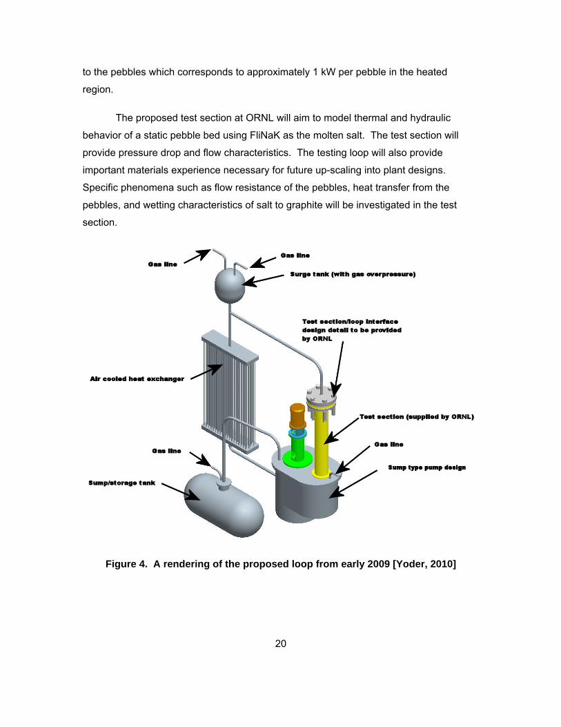
The proposed test section at ORNL will aim to model thermal and hydraulic
behavior of a static pebble bed using FliNaK as the molten salt. The test section will
provide pressure drop and flow characteristics. The testing loop will also provide
important materials experience necessary for future up-scaling into plant designs.
Specific phenomena such as flow resistance of the pebbles, heat transfer from the
pebbles, and wetting characteristics of salt to graphite will be investigated in the test
section.
Figure 4. A rendering of the proposed loop from early 2009 [Yoder, 2010]

21
2.2 Test Operations
Startup design includes a sump storage tank per Figure 4 such that the coolant
can gravity drain to the sump in case of shutdown, preventing inadvertent solidification in
the loop. The storage tank will need to be preheated to 454ºC to melt the salt before
pump operation. During non-operational periods, the salt will solidify; however, unlike
water, molten salts contract upon freezing, so pump components will not be damaged.
Trace heating (heating of the flow lines) will be used on the pipes to increase their
temperature prior to loop filling to prevent thermal shocks. Current plans will utilize
commercially available heating tape to preheat the loop to 600ºC. A cleaning
agent/solvent will be used prior to initial startup for decontamination of inner flow
surfaces. A vacuum pump will evacuate the loop before startup, and a sump tank cover
gas (argon) will provide pressure to force the salt into the loop through a dipper tube.
2.3 Instrumentation and Controls
High temperature instrumentation has been developed and demonstrated in lab
environments; however, little of that technology is currently commercially available due
to a small market audience for high temperature systems. This therefore requires
custom technology for which long-term reliability and drift has not been identified. The
large scope of this project has been to identify available technology and customize it for
implementation in the loop. A portion of this work has been performed using previous
trials available through literature and utilizing resources made available by ORNL and
UT to support customization.
Temperature measurements for the loop will be provided with commercially
available K-type thermocouples. For long-term solutions for the harsh environments in a
plant design, other technologies such as fiber-optic coupled pyrometry and Fizeau
cavity-type thermometers are commercially available, and could be investigated for
future applications.
Ultrasonic flow meters will be used for the measurement of flow through the loop.
Ultrasonic wave-guides will be used to maintain a mechanical standoff in order to protect
the electronic components from the high temperatures. The technology for this concept

22
is well developed; in that, there will be essentially no difference between the electronics
for applications in high temperature water-cooled and molten salt cooled reactors. An
alternate option would be the use of a Venturi-type flow meter which requires two
pressure measurements.
Ultrasonic technology will be used for level sensing in the heat up tank. The level
will also be measured utilizing two rods (one unheated, one heated) lined with
thermocouples. The thermocouples immersed in the salt will not show a difference in
temperature; while, the thermocouples outside the salt, in argon, will show different
temperature readings. Using this knowledge, the level can be known within a range of
the spacing of the thermocouples.
2.4 Preliminary Calculations
An initial pressure drop and flow analysis was performed using the early
drawings of the proposed test loop provided by ORNL. These calculations established
performance limits for the pressure instruments. Relationships for the modeling of
packed spherical beds were modeled in Matlab (Appendix B) with the intention of
recalculating when the completed designs were in place. The final designs have not
been completed to date, so the code and calculations are a resource for quick
comparison of future modeling using software such as Relap5. The thermophysical
properties of FLiNaK at 700ºC have been reported by Williams in an assessment of
potential molten salts.
Table 1. Thermophysical properties of FLiNaK at 700ºC [Williams]
Property Value
Melting point 454 ºC
pCp , Volumetric Heat Capacity 0.91 cal/cm3- ºC
, Viscosity 2.9 cP
k, Thermal conductivity 0.92 W/(m-K)
ρ, Density 2.02 g/cm3

23
It was assumed that insulation was sufficient such that heat leakage through the
pipes would not alter the energy balance. The functional parameters for the air to salt
heat exchanger are given in Table 2.
The estimated loop dimensions were given by ORNL and are provided in
Appendix A. Two separate methods were used to determine the pressure drop through
the loop. A Matlab code was written which utilizes classic heat transport theory to
determine the pressure drops in the pipes, heat exchanger, and test section. A second
method used Fathom 6.0, a program designed to calculate pressure drops in general
fluid flow systems. Since both programs utilized classic heat transfer theory, many of
the calculations were the same. Fathom cannot calculate pressure drops through a
pebble bed so a K-factor was utilized that was derived from the Matlab code
implementation of pebble bed models.
Table 2. Functional parameters for modeling the pressure drop in the air to salt heat exchanger.
Parameter Value
Mass Flow Rate 4.5 kg/s
HX Performance 100 kW
Inlet Molten Salt Temperature 700 ºC
Outlet Molten Salt Temperature 688.2 ºC
Inlet Air Temperature 20 ºC
Outlet Air Temperature 65 ºC
Thickness of Channel Walls 1 mm
For the test section pressure drop, two theories were examined that model
pebble bed flow, the Ergun relation and Idelchik. The Ergun relation [Bird]:
3
20
322
20 )1()1(150
pspsD
v
D
v
L
P
(2.4.1)
The Idelchik relation [Idelchik]:

24
2
2o
drop
vP (2.4.2)
pD
l07.02.4
)3.0Re
3
Re
30(
53.1
(2.4.3)
pDw1
)1(
45.0Re
(2.4.4)
9060;cos21)cos1(6
1
(2.4.5)
The porosity is a complicating issue without knowing the complete pebble bed
design details. All previous work assumed a bed length of 111.6 cm with diameter of 15
cm. however, if this were the case the porosity would be approximately 0.893 with the
assumed maximum of 150 pebbles. Porosity is almost always less than 0.5 for spheres.
With pebbles 3 cm in diameter, a single plane of 150 pebbles spanning the bed diameter
would only reach 88.9 cm. To fill a 111.6 cm long pebble bed, more than 800 pebbles
would be needed for a porosity of 0.40, which appears to be the average for a randomly
packed pebble bed. The test loop could also be slightly different considering the bed
diameter is only 5 pebble diameters wide. This will present challenges in choosing a
porosity since wall effects will be significant.
It was assumed that the pebble bed length was 111.6 cm with a porosity of 0.45
(79°) considering the small diameter of the test section. Although this could be higher
with wall effects, the maximum achievable porosity with 90° packing angles is 0.48.
Using these numbers, it has been assumed that there are 766 pebbles. Using the Ergun
equation this gives a pressure drop as a result of packing of 13 kPa and a total with the
addition of entrance, exit, and gravitational pressure losses of 35 kPa. With this setup,
the Idelchik equations will give a pressure drop of 8.45 kPa and total drop of 31 kPa.
The ORNL requirements list a test section pressure drop of 0.1 MPa. The Idelchik
equations, for a packing angle of 60°, give approximately 0.1072 MPa which compares
favorably to the ORNL results. A 60° packing angle would be the maximum packing

25
angle possible and corresponds to a porosity of 0.2595. The Ergun equation, for a
porosity of 0.2595 gives a total pressure loss of 0.11 MPa.
So the pressure drop was assumed to be 0.1 MPa using the Fathom code since
it cannot calculate pressure losses in a bed. To do this a K-factor of 5,271 was used for
a pressure drop of 0.1 MPa at full flow. The K-factor model in Fathom scales pressure
drop with bed mass flow to the power of two, consistent with the Ergun model.
A heat exchanger that could remove 100 kW was assumed based off preliminary
conditions given by ORNL. The configuration chosen was 30 flattened ducts of width
22.9 cm, length 132 cm, 0.635 cm thick, and with a wall thickness of 1mm. Convective
and radiative heat transfer was considered [Schlunder]. The thermal emissivity of the
MONICOR or Hastelloy is not known. So a design with excess heat sink which ranged
from 99 kW at an emissivity of 0.6 to 112 kW as taken black was considered. 20ºC was
assumed for T(∞,rad). The hydraulic diameter of these ducts is 1.27 cm which was used
in Fathom as the heat exchanger pipe diameter.
The overall pumping power needed according to Fathom, per Figure 5, is 318 W
which corresponds to a mass flow rate of 4.5 kg/s and a FliNaK salt pressure head of
23.63 feet (143 kPa).

26
Figure 5. Fathom model utilizing preliminary loop dimensions.
27
Chapter 3. High Temperature Pressure Sensor Design Constraints
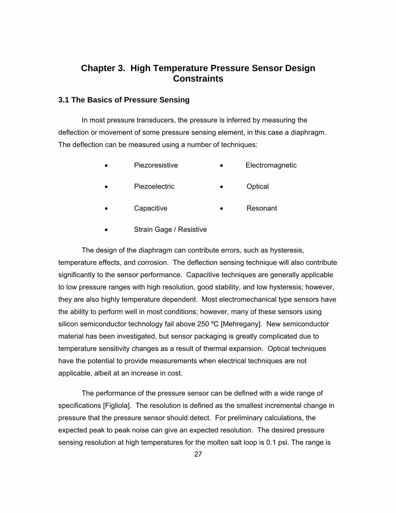
3.1 The Basics of Pressure Sensing
In most pressure transducers, the pressure is inferred by measuring the
deflection or movement of some pressure sensing element, in this case a diaphragm.
The deflection can be measured using a number of techniques:
Piezoresistive Electromagnetic
Piezoelectric Optical
Capacitive Resonant
Strain Gage / Resistive
The design of the diaphragm can contribute errors, such as hysteresis,
temperature effects, and corrosion. The deflection sensing technique will also contribute
significantly to the sensor performance. Capacitive techniques are generally applicable
to low pressure ranges with high resolution, good stability, and low hysteresis; however,
they are also highly temperature dependent. Most electromechanical type sensors have
the ability to perform well in most conditions; however, many of these sensors using
silicon semiconductor technology fail above 250 ºC [Mehregany]. New semiconductor
material has been investigated, but sensor packaging is greatly complicated due to
temperature sensitivity changes as a result of thermal expansion. Optical techniques
have the potential to provide measurements when electrical techniques are not
applicable, albeit at an increase in cost.
The performance of the pressure sensor can be defined with a wide range of
specifications [Figliola]. The resolution is defined as the smallest incremental change in
pressure that the pressure sensor should detect. For preliminary calculations, the
expected peak to peak noise can give an expected resolution. The desired pressure
sensing resolution at high temperatures for the molten salt loop is 0.1 psi. The range is
28
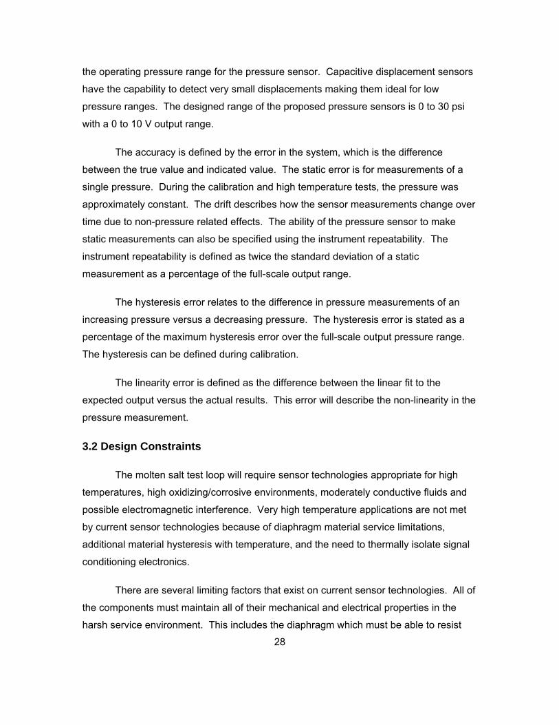
the operating pressure range for the pressure sensor. Capacitive displacement sensors
have the capability to detect very small displacements making them ideal for low
pressure ranges. The designed range of the proposed pressure sensors is 0 to 30 psi
with a 0 to 10 V output range.
The accuracy is defined by the error in the system, which is the difference
between the true value and indicated value. The static error is for measurements of a
single pressure. During the calibration and high temperature tests, the pressure was
approximately constant. The drift describes how the sensor measurements change over
time due to non-pressure related effects. The ability of the pressure sensor to make
static measurements can also be specified using the instrument repeatability. The
instrument repeatability is defined as twice the standard deviation of a static
measurement as a percentage of the full-scale output range.
The hysteresis error relates to the difference in pressure measurements of an
increasing pressure versus a decreasing pressure. The hysteresis error is stated as a
percentage of the maximum hysteresis error over the full-scale output pressure range.
The hysteresis can be defined during calibration.
The linearity error is defined as the difference between the linear fit to the
expected output versus the actual results. This error will describe the non-linearity in the
pressure measurement.
3.2 Design Constraints
The molten salt test loop will require sensor technologies appropriate for high
temperatures, high oxidizing/corrosive environments, moderately conductive fluids and
possible electromagnetic interference. Very high temperature applications are not met
by current sensor technologies because of diaphragm material service limitations,
additional material hysteresis with temperature, and the need to thermally isolate signal
conditioning electronics.
There are several limiting factors that exist on current sensor technologies. All of
the components must maintain all of their mechanical and electrical properties in the
harsh service environment. This includes the diaphragm which must be able to resist
29
corrosive environments and mechanical property changes at 700ºC. The signal must be
compensated to address non-linearity in the relationship between pressure and
temperature. This is a demanding task at very high temperatures with current sensor
technologies. The most common way of dealing with high temperatures is protecting the
electronics from high temperatures by an intermediary fluid transmission line, typically
using a fluid with small density changes with temperature that is liquid throughout the
temperature range. However, as mentioned previously, the impulse line method was not
acceptable for this application.
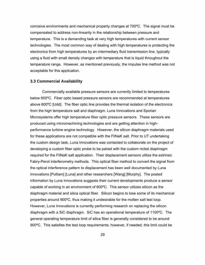
3.3 Commercial Availability
Commercially available pressure sensors are currently limited to temperatures
below 600ºC. Fiber optic based pressure sensors are recommended at temperatures
above 600ºC [Udd]. The fiber optic line provides the thermal isolation of the electronics
from the high temperature salt and diaphragm. Luna Innovations and Sporian
Microsystems offer high temperature fiber optic pressure sensors. These sensors are
produced using micromachining technologies and are getting attention in high-
performance turbine engine technology. However, the silicon diaphragm materials used
for these applications are not compatible with the FliNaK salt. Prior to UT undertaking
the custom design task, Luna Innovations was contacted to collaborate on the project of
developing a custom fiber optic probe to be paired with the custom nickel diaphragm
required for the FliNaK salt application. Their displacement sensors utilize the extrinsic
Fabry-Perot interferometry methods. This optical fiber method to convert the signal from
the optical interference pattern to displacement has been well documented by Luna
Innovations [Pulliam] [Luna] and other researchers [Wang] [Murphy]. The posted
information by Luna Innovations suggests their current developments produce a sensor
capable of working in an environment of 600ºC. This sensor utilizes silicon as the
diaphragm material and silica optical fiber. Silicon begins to lose some of its mechanical
properties around 900ºC, thus making it undesirable for the molten salt test loop.
However, Luna Innovations is currently performing research on replacing the silicon
diaphragm with a SiC diaphragm. SiC has an operational temperature of 1100ºC. The
general operating temperature limit of silica fiber is generally considered to be around
900ºC. This satisfies the test loop requirements; however, if needed, this limit could be

30
extended through use of sapphire fibers. Packaging of the sensor would also be
required to withstand the harsh environment.
An initial potential collaboration between UT and Luna would have contracted
Luna to provide assistance with the "internal" workings of the pressure sensor for the
molten salt test loop. Luna would have provided technical support and the
interferometer readout equipment. This includes details such as data analysis and
measurement readout support. Typically these electronics are rented for a period of
around three months depending on availability. UT with the support of ORNL and Luna
was to design and fabricate the sensing diaphragm and other materials for the fiber optic
sensor. This partnership was not followed when the budget proposed by Luna fell
outside the planned budget provided by UT and ORNL. Similar discussions were also
held with Sporian Microsystems, INC, another fiber optic displacement sensor
manufacturer, with similar results [Sporian].
31
Chapter 4. Interferometric Fiber Optic Pressure Sensor
4.1 Fundamentals of Fiber Optic Sensing
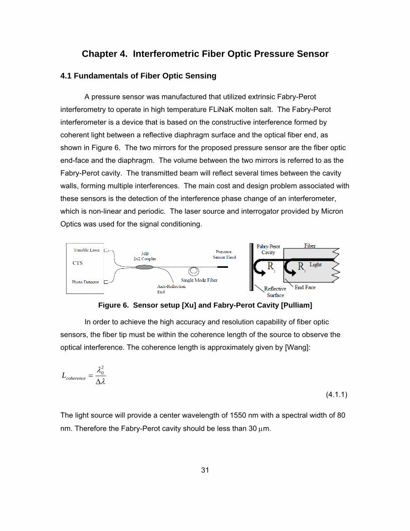
A pressure sensor was manufactured that utilized extrinsic Fabry-Perot
interferometry to operate in high temperature FLiNaK molten salt. The Fabry-Perot
interferometer is a device that is based on the constructive interference formed by
coherent light between a reflective diaphragm surface and the optical fiber end, as
shown in Figure 6. The two mirrors for the proposed pressure sensor are the fiber optic
end-face and the diaphragm. The volume between the two mirrors is referred to as the
Fabry-Perot cavity. The transmitted beam will reflect several times between the cavity
walls, forming multiple interferences. The main cost and design problem associated with
these sensors is the detection of the interference phase change of an interferometer,
which is non-linear and periodic. The laser source and interrogator provided by Micron
Optics was used for the signal conditioning.
Figure 6. Sensor setup [Xu] and Fabry-Perot Cavity [Pulliam]
In order to achieve the high accuracy and resolution capability of fiber optic
sensors, the fiber tip must be within the coherence length of the source to observe the
optical interference. The coherence length is approximately given by [Wang]:
20
coherenceL
(4.1.1)
The light source will provide a center wavelength of 1550 nm with a spectral width of 80
nm. Therefore the Fabry-Perot cavity should be less than 30 m.
32
4.2 Flat and Rigid Diaphragm
The diaphragm design for the fiber optic probe was chosen as flat with rigid
perimeter because of its simplicity. The fiber optic techniques being used are capable of
reading displacement in the nanometer range. The material considered was nickel or an
almost pure nickel alloy.
Table 3. Nickel properties relevant for diaphragm design
Material Young’s Modulus Poisson’s Ratio
Nickel 161 GPa 0.28
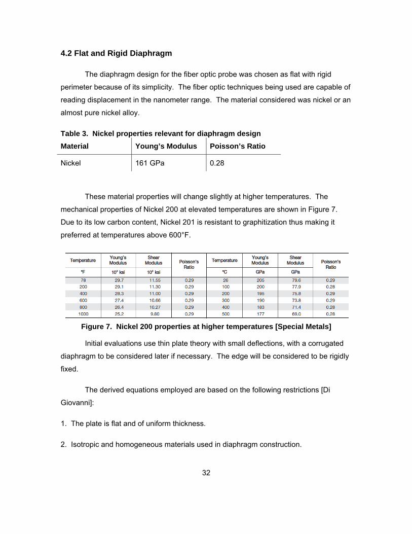
These material properties will change slightly at higher temperatures. The
mechanical properties of Nickel 200 at elevated temperatures are shown in Figure 7.
Due to its low carbon content, Nickel 201 is resistant to graphitization thus making it
preferred at temperatures above 600°F.
Figure 7. Nickel 200 properties at higher temperatures [Special Metals]
Initial evaluations use thin plate theory with small deflections, with a corrugated
diaphragm to be considered later if necessary. The edge will be considered to be rigidly
fixed.
The derived equations employed are based on the following restrictions [Di
Giovanni]:
1. The plate is flat and of uniform thickness.
2. Isotropic and homogeneous materials used in diaphragm construction.

33
3. The maximum deflection allowed is one-fifth of the diaphragm thickness.
4. All loads are applied normally to the plane of the diaphragm.
5. The plate is not stressed beyond the elastic limit.
6. The plate thickness should be no more than 20% of the diameter.
7. The plate deflection is due mostly to bending such that the median plane of the plate
endures no tensile forces.
The three important variables considered are: radius of the diaphragm, thickness
of the diaphragm, and cavity height. The theory of this design follows the reference of Di
Giovanni.
A Matlab code given in Appendix C was written that allows ease of design
performance assessment. Initial analysis investigates a diaphragm approximately 1/2” in
diameter since these are the dimensions of the pressure access tube. The deflection of
the diaphragm as a function of pressure and radial distance is given by:
2223
2
)(16
)1(3ra
Eh
Py
(4.2.1)
The maximum deflection will occur at the center of the diaphragm:
3
42
16
)1(3
Eh
Payo
(4.2.2)
The one-fifth rule allows for the diaphragm to be in the linear range of deflection
versus pressure, often referred to as small deflection theory. This can be used to find a
diaphragm thickness:
andhyo 51
(4.2.3)

34
thenEh
Payo 3
42
16
)1(3 (4.2.4)
4
42
16
)1(15
E
Pah
(4.2.5)
The sensitivity of the diaphragm is given as the amount of displacement per unit
of applied pressure. The sensitivity at the center is the place of concern since it is the
measurement point for the displacement sensor. The linear operating range of the
diaphragm follows the relation:
3
420
16
)1(3
Eh
a
P
yY
(4.2.6)
The results of these calculations using properties from Figure 7 are provided in
Table 4.
Table 4. Diaphragm displacement versus applied pressure
Max Pressure: 29 psi Diaphragm Radius: 0.25 in. (6.4 mm)
Diaphragm Thickness:
0.0076 in (0.19 mm )
Maximum Deflection:
0.0015 in (0.039 mm)
Sensitivity: 1.34 m/psi (linear within 0 to 29 psi range)
The deflection profile in Figure 8 is calculated using Matlab, and the code is
presented in Appendix C:

35
0 0.1 0.2 0.3 0.4 0.5 0.6 0.7 0.8 0.9 10
0.1
0.2
0.3
0.4
0.5
0.6
0.7
0.8
0.9
1
Radial Distance (r/a)
Def
lect
ion
(y/y
0)
Figure 8. Diaphragm deflection profile
Equations 4.2.1 through 4.2.6 are satisfactory for bending stresses only. Higher
pressures may be accounted for as well, although the response to pressure changes is
no longer linear. The general characteristic equation for a flat diaphragm can be used to
account for both bending and tensile stresses seen in larger loads.
For small displacements:
h
y
Eh
Pa 024
4
)1(3
16
(4.2.7)
For larger displacements:
3
30
4
4
)1(3
7
h
y
Eh
Pa
(4.2.8)
By method of superposition:
36
3
300
3
300
24
4
23.390.5)1(3
7
)1(3
16
h
y
h
y
h
y
h
y
Eh
Pa
(4.2.9)
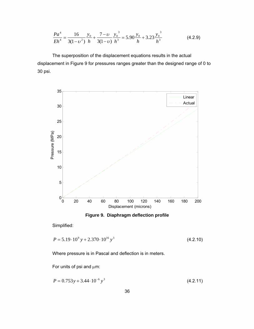
The superposition of the displacement equations results in the actual
displacement in Figure 9 for pressures ranges greater than the designed range of 0 to
30 psi.
0 20 40 60 80 100 120 140 160 180 2000
5
10
15
20
25
30
35
Displacement (microns)
Pre
ssur
e (M
Pa)
Linear
Actual
Figure 9. Diaphragm deflection profile
Simplified:
3169 10370.21019.5 yyP (4.2.10)
Where pressure is in Pascal and deflection is in meters.
For units of psi and m:
361044.3753.0 yyP (4.2.11)

37
The maximum radial stress is at the edge and is given by:
2
2
max, 4
3
h
PaR (4.2.12)
The maximum tangential stress is at the center of the diaphragm and is given by:
2
2
max, )1(8
3
h
PaT (4.2.13)
At the center the tangential and radial stresses are equal. The tangential stress
at the edge is given by:
2
2
4
3
h
PaT (4.2.14)
0 0.1 0.2 0.3 0.4 0.5 0.6 0.7 0.8 0.9 1-1.5
-1
-0.5
0
0.5
1
1.5
2x 10
7
Radial Distance (r/a)
Str
ess(
Pa)
Radial
Tangential
Figure 10. Diaphragm stress profile
38
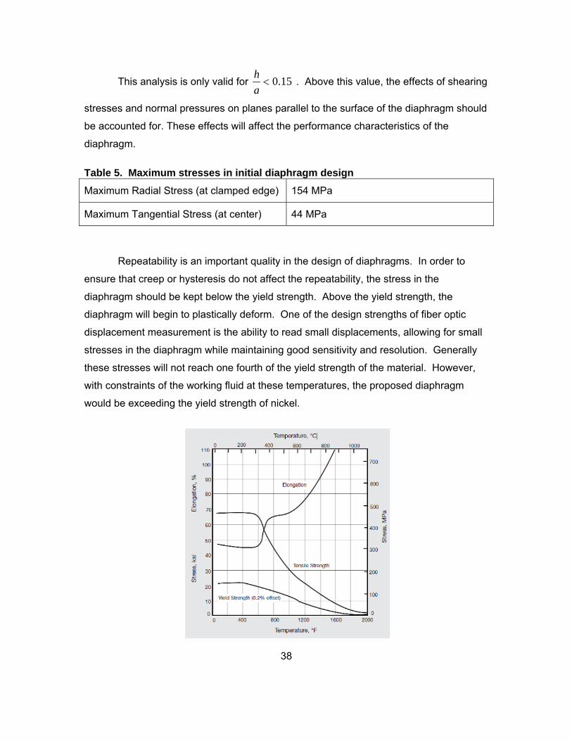
This analysis is only valid for 15.0a
h . Above this value, the effects of shearing
stresses and normal pressures on planes parallel to the surface of the diaphragm should
be accounted for. These effects will affect the performance characteristics of the
diaphragm.
Table 5. Maximum stresses in initial diaphragm design
Maximum Radial Stress (at clamped edge) 154 MPa
Maximum Tangential Stress (at center) 44 MPa
Repeatability is an important quality in the design of diaphragms. In order to
ensure that creep or hysteresis do not affect the repeatability, the stress in the
diaphragm should be kept below the yield strength. Above the yield strength, the
diaphragm will begin to plastically deform. One of the design strengths of fiber optic
displacement measurement is the ability to read small displacements, allowing for small
stresses in the diaphragm while maintaining good sensitivity and resolution. Generally
these stresses will not reach one fourth of the yield strength of the material. However,
with constraints of the working fluid at these temperatures, the proposed diaphragm
would be exceeding the yield strength of nickel.

39
Figure 11. Nickel 200 material properties [Special Metals]
From Figure 11, one can see that the radial stresses of 144 MPa in Figure 10
and Table 5 will cause plastic deformation in the diaphragm. Therefore, the diaphragm
will need to be altered. This could be done two ways: 1) thicken the diaphragm, thus
reducing the stresses but also reducing the sensitivity, or 2) use a nickel alloy which is
designed to increase strength by increasing the chrome content, which also increases
corrosion susceptibility.
Nickel has been shown to have the best resistance to corrosion in a FLiNaK
environment. Therefore, it would still be the material of choice if the internal stresses of
the diaphragm can be kept in the elastic region. In order to do this, the thickness will be
increased to lower the stresses in the diaphragm. This will increase the linear pressure
range but the diaphragm sensitivity will decrease. The target stress would be at the
0.2% offset yield strength or preferably the 0.01% offset proof stress. The 0.2% offset
yield strength for Nickel 200 is approximately 30 MPa.
40
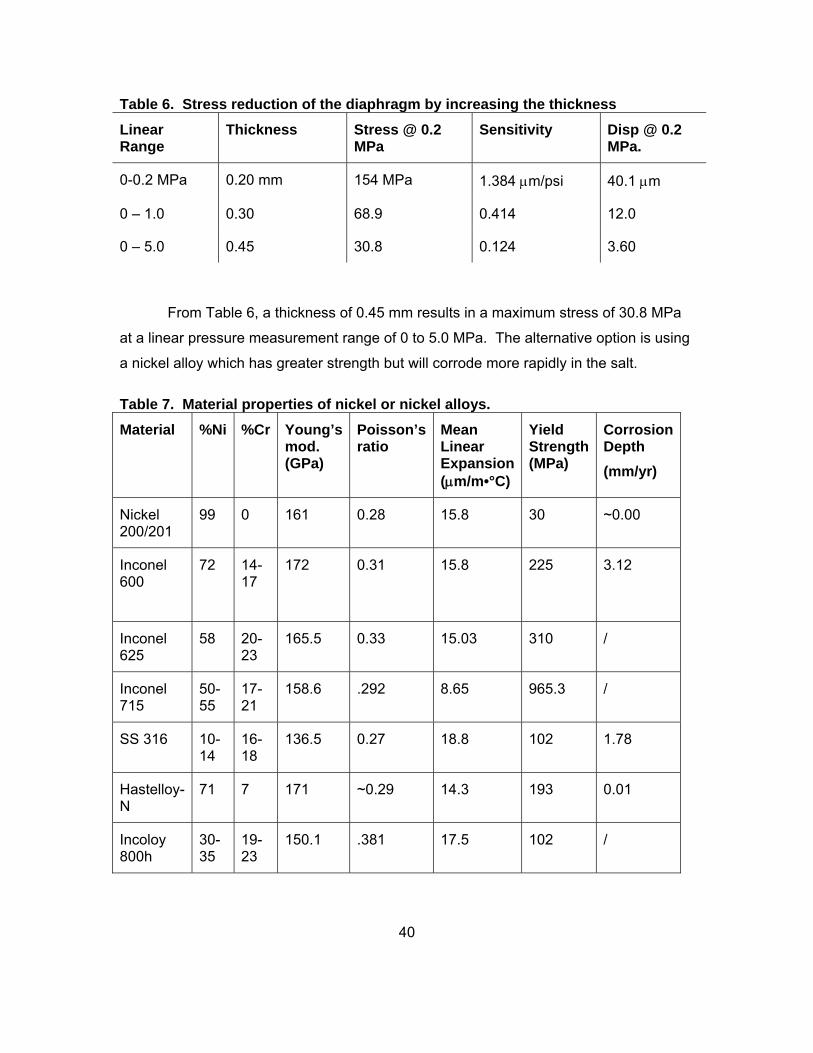
Table 6. Stress reduction of the diaphragm by increasing the thickness
Linear Range
Thickness Stress @ 0.2 MPa
Sensitivity Disp @ 0.2 MPa.
0-0.2 MPa 0.20 mm 154 MPa 1.384 m/psi 40.1 m
0 – 1.0 0.30 68.9 0.414 12.0
0 – 5.0 0.45 30.8 0.124 3.60
From Table 6, a thickness of 0.45 mm results in a maximum stress of 30.8 MPa
at a linear pressure measurement range of 0 to 5.0 MPa. The alternative option is using
a nickel alloy which has greater strength but will corrode more rapidly in the salt.
Table 7. Material properties of nickel or nickel alloys.
Material %Ni %Cr Young’s mod. (GPa)
Poisson’s ratio
Mean Linear Expansion (m/m•°C)
Yield Strength (MPa)
Corrosion Depth
(mm/yr)
Nickel 200/201
99 0 161 0.28 15.8 30 ~0.00
Inconel 600
72 14-17
172 0.31 15.8 225 3.12
Inconel 625
58 20-23
165.5 0.33 15.03 310 /
Inconel 715
50-55
17-21
158.6 .292 8.65 965.3 /
SS 316 10-14
16-18
136.5 0.27 18.8 102 1.78
Hastelloy-N
71 7 171 ~0.29 14.3 193 0.01
Incoloy 800h
30-35
19-23
150.1 .381 17.5 102 /

41
For linear pressure range of 0.0 MPa to 0.2MPa, several nickel alloys are
considered. From the results, the sensitivities are all similar due to the similar modulus
of these alloys.
Table 8. Results of diaphragm design for each considered alloy
Material Thickness (mm)
Stress @0.2MPa (MPa)
Actual Stress / Yield Stress
Sensitivity
(m/psi)
Disp @0.2 MPa. (m)
Ni 201 0.20 149.0 4.97 1.41 40.9
Inconel 600
0.20 155.1 0.689 1.34 40.0
Inconel 625
0.199 156.2 0.504 1.37 39.8
Inconel 715
0.204 148.0 0.153 1.412 41.0
SS 316 0.213 136.4 1.34 1.47 42.6
Hastelloy-N
0.20 154.0 0.798 1.39 40.2
Incoloy 800h
0.204 149.0 1.46 1.41 40.8
For those materials where the ratio of the actual stress to yield stress is above
1.0, the thickness will need to be increased. In order to get each diaphragm design
below their material’s yield stress, the thickness and sensitivities were solved using the
yield stress as the design constraint, which is easily accomplished by manipulating
equations 4.2.5 and 4.2.12 into:
max,
2
4
3
R
Pah
(4.2.15)
Table 9 results demonstrate how the stronger alloys allow greater sensitivity in
the diaphragm. The displacements at the expected pressure are often several factors
greater than that for pure nickel. However, the corrosion in the FLiNaK salt of the

42
diaphragms would be able to penetrate through the thickness within a month for most
alloys. The Hastelloy-N would be an ideal material; however, it is not commercially
available for a project of this type.
43
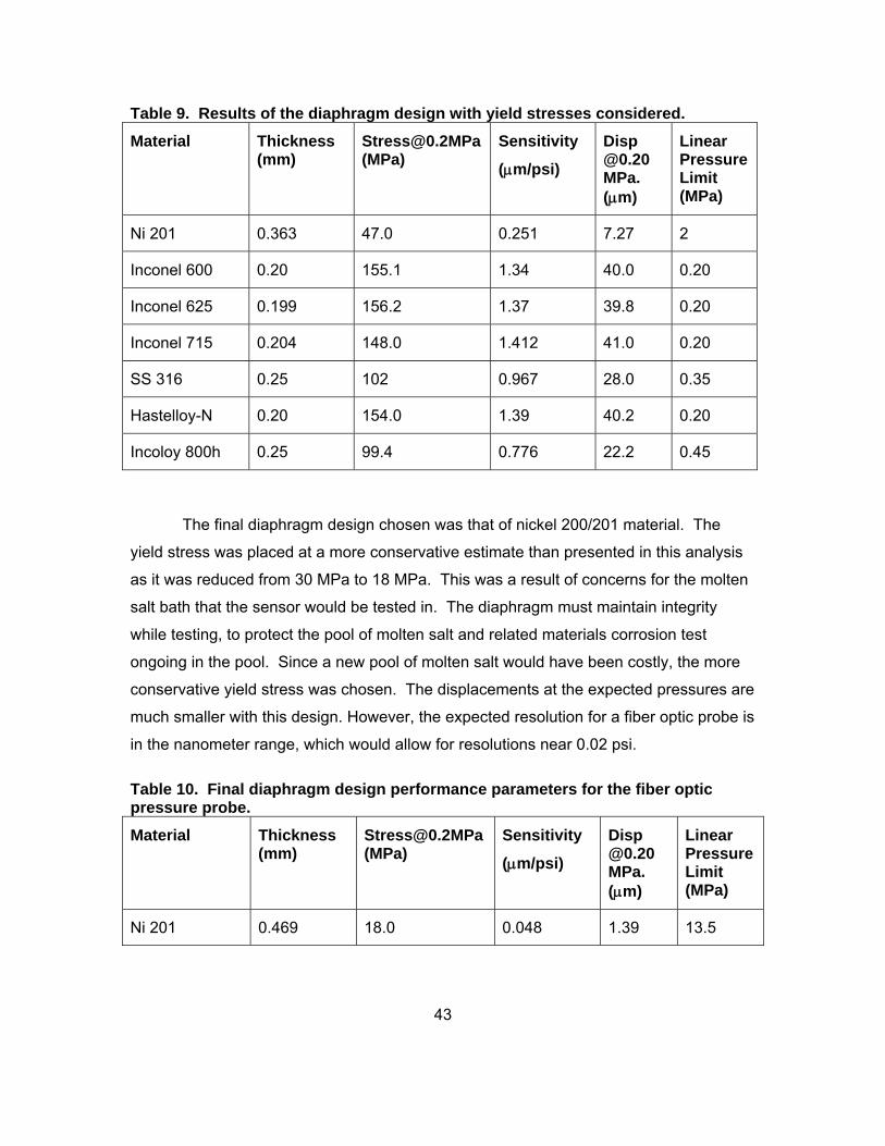
Table 9. Results of the diaphragm design with yield stresses considered.
Material Thickness (mm)
[email protected] (MPa)
Sensitivity
(m/psi)
Disp @0.20 MPa. (m)
Linear Pressure Limit (MPa)
Ni 201 0.363 47.0 0.251 7.27 2
Inconel 600 0.20 155.1 1.34 40.0 0.20
Inconel 625 0.199 156.2 1.37 39.8 0.20
Inconel 715 0.204 148.0 1.412 41.0 0.20
SS 316 0.25 102 0.967 28.0 0.35
Hastelloy-N 0.20 154.0 1.39 40.2 0.20
Incoloy 800h 0.25 99.4 0.776 22.2 0.45
The final diaphragm design chosen was that of nickel 200/201 material. The
yield stress was placed at a more conservative estimate than presented in this analysis
as it was reduced from 30 MPa to 18 MPa. This was a result of concerns for the molten
salt bath that the sensor would be tested in. The diaphragm must maintain integrity
while testing, to protect the pool of molten salt and related materials corrosion test
ongoing in the pool. Since a new pool of molten salt would have been costly, the more
conservative yield stress was chosen. The displacements at the expected pressures are
much smaller with this design. However, the expected resolution for a fiber optic probe is
in the nanometer range, which would allow for resolutions near 0.02 psi.
Table 10. Final diaphragm design performance parameters for the fiber optic pressure probe.
Material Thickness (mm)
[email protected] (MPa)
Sensitivity
(m/psi)
Disp @0.20 MPa. (m)
Linear Pressure Limit (MPa)
Ni 201 0.469 18.0 0.048 1.39 13.5

44
Figure 12. Nickel diaphragm dimensions and conceptual drawing (dimensions in
inches)
4.3 First Design
A first design of a fiber optic pressure sensor was developed for a molten salt
very high temperature environment (700°C). The sensor was placed in a molten salt
bath through a 0.50” tube. The following components were machined consistent with
Figure 13 using the following materials procured by UTK:
Nickel 200/201 1/2 IN diameter, 5 FT length Round Bar (later found to be steel)
Nickel 200 0.250" OD x .028" Wall (Seamless) tube
Nickel 200 0.500” OD x 0.028” Wall (Seamless) tube; 20’
The machined components were then sent to ORNL for laser tack welding where
specified in assembly plans per Appendix D. The machined components were inspected
to specifications post-welding. Circumferential arc welding was performed on the end-
cap and outer 0.500” OD x 0.028” wall tubing.
The completed machining and welding included two final components: the outer
18” long x 0.028” wall tubing arc welded to an end cap that houses a nickel spacer tack
welded to the end-cap and the inner 18” long x 0.028” wall tubing tack welded to the
housing for the optical fiber.
45
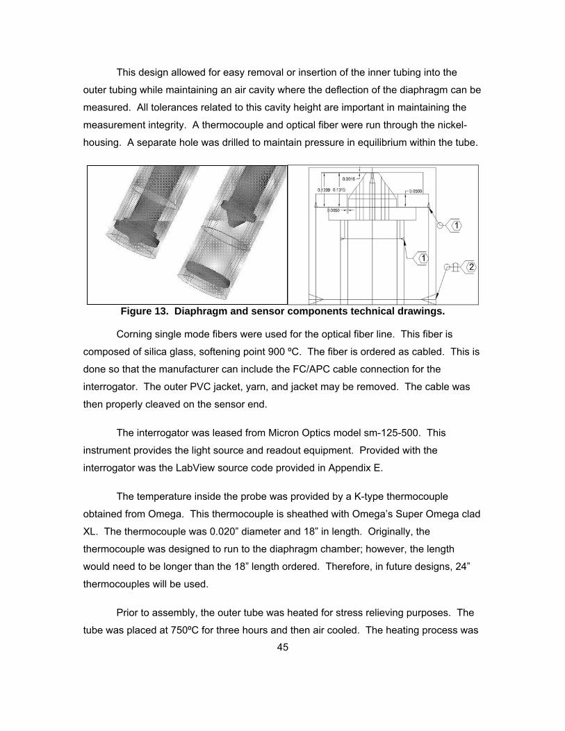
This design allowed for easy removal or insertion of the inner tubing into the
outer tubing while maintaining an air cavity where the deflection of the diaphragm can be
measured. All tolerances related to this cavity height are important in maintaining the
measurement integrity. A thermocouple and optical fiber were run through the nickel-
housing. A separate hole was drilled to maintain pressure in equilibrium within the tube.
Figure 13. Diaphragm and sensor components technical drawings.
Corning single mode fibers were used for the optical fiber line. This fiber is
composed of silica glass, softening point 900 ºC. The fiber is ordered as cabled. This is
done so that the manufacturer can include the FC/APC cable connection for the
interrogator. The outer PVC jacket, yarn, and jacket may be removed. The cable was
then properly cleaved on the sensor end.
The interrogator was leased from Micron Optics model sm-125-500. This
instrument provides the light source and readout equipment. Provided with the
interrogator was the LabView source code provided in Appendix E.
The temperature inside the probe was provided by a K-type thermocouple
obtained from Omega. This thermocouple is sheathed with Omega’s Super Omega clad
XL. The thermocouple was 0.020” diameter and 18” in length. Originally, the
thermocouple was designed to run to the diaphragm chamber; however, the length
would need to be longer than the 18” length ordered. Therefore, in future designs, 24”
thermocouples will be used.
Prior to assembly, the outer tube was heated for stress relieving purposes. The
tube was placed at 750ºC for three hours and then air cooled. The heating process was

46
done in an open furnace. Ideally, this would be performed in an inert gas to prevent
oxidation. Due to time constraints, this was not done, and the oxide layer that formed
during the stress relieving process was removed.
There were many attempts at assembling the sensor. The most troubling issue
was maintaining the integrity of the fiber optic cleave. The fiber had to be cleaved
several times which was performed by the telecommunication employees from the
University of Tennessee. The quality of the cleave can also affect the sensor’s
performance.
The first change to design was the inclusion of an argon inlet and outlet. This
included the addition of an insert that runs to the outer edge of the fiber nickel tip. This
also required that an end cap for the sensor with passages for the fiber, thermocouple,
1/16” argon inlet, and 1/8” argon outlet had to be fabricated. Initially, the argon outlet
was thought to be not necessary due to the small amount of argon running through the
sensor probe. However, it was later recommended by Electrochemical Systems (ECS)
and accommodated.
Initially, the inner tube was laser tack welded to the conical cap to hold the fiber
tip. It was also unclear if the fiber tip was cleaved. It was thought that the coating
surrounding the silica clad was not able to be removed without damaging the fiber.
Therefore, the insertion hole for the fiber tip was widened to accomodate the fiber and
coating. The initial expectation was that the fiber would be bare. After multiple attempts
at drawing the fiber through the orifice, the tack welds that connected the nickel conical
tip were removed to ease the installation process.
After the tack welds were removed, assembly was made possible. It was also
realized at this time that the fiber tip needed to be cleaved at a 90º angle. The tools for
fiber cleaving are expensive, so the telecommunication employees were contacted. The
cleaved fiber tips are very fragile and only 125 μm in diameter. Therefore, it was ideal to
have the tip already inserted through the guide tube before cleaving. The final assembly
was done with a fiber that had been moved in to and out of the nickel tubing, providing
opportunity for damage. A redesign of the sensor could better accommodate assembly.
47
The fiber needs to be at a 90º angle with the diaphragm for accurate
displacement measurement. The fiber also must be aligned at the center of the
diaphragm. This was not well facilitated with the modified hole for the optical fiber.
Fiberglass stove gasket cement was used for the fiber to nickel holder adhesion.
Hypodermic needles were used to place the cement near the tip. In order to get good
adhesion, cement was filled through the fiber guide hole. The fiber was then slid through
the hole and cleaned with a cloth at the tip. The guide hole should be the diameter of
the bare fiber in future designs, such that the tip is held in place and cement could then
be applied higher on the fiber. This will also help ensure that the fiber tip is properly
aligned with the tip of the nickel holder. Accurate measurements require the fiber tip to
be less than 30 μm from the diaphragm. This fiber holder design is critical to maintaining
these dimensions.
In the final attempt, the entire nickel holder was filled with cement, while two
hypodermic needles maintained the holes for the argon inlet. The fiber was then run
through the cement and insertion hole. After being cleaned, the fiber was gently pushed
with a level metal plate back until it was flat with the holder. The tip holder was then
placed into the ¼” nickel tubing. When the cement was partially dry, the two hypodermic
needles were pulled from the holder. Unfortunately, the fiber was not perfectly aligned to
the center of the diaphragm such that pressure measurements would not perfectly follow
the theoretical performance predictions for the diaphragm.
4.4 Molten Salt Bath Testing Facility
The pressure sensor testing facility consisted of a molten salt bath approximately
15" in depth that was provided by Electrochemical Systems (ECS) of Oak Ridge and
shown in Figure 14. The molten salt bath included a nickel heater rod and an argon
cover system that provided a few psi of over-pressure. During the testing stages, ORNL
designed a new top flange to accommodate the testing of the pressure sensor as shown
in Figure 15. This test would be run simultaneously with material compatibility testing.
Therefore, it was important to maintain the integrity of the diaphragm. A defect or leak in
the diaphragm could expose the center of the salt bath to air compromising the purity of
the salt. This would also result in compromising the materials testing. To prevent this,

48
the argon supply inside the pressure sensor would prevent potential air leakage into the
salt.
Figure 14. CAD representation of new top flange and with the older top flange
Figure 15. The testing facility and setup showing the pressure sensor position
4.5 Testing Results
Prior to each cleave during the assembly process data was taken to test the
integrity of the fiber cleaves. The apparatus is as shown in Figure 16. The distance
between the fiber tip and diaphragm was measured with a machinist ruler.

49
Figure 16. Calibration apparatus during assembly
From observing the readout provided by the Micron Optics LabView source code, it is
obvious if the fiber is reading a reflection. From Figure 17, the wavelike motion, or fringe
pattern, in the reflective intensity (top-left) and the strong peaks in the amplitude
(bottom-center) indicate a properly working sensor.
Figure 17. A properly working signal from the fiber optic diaphragm displacement
measurement

50
For a failed displacement measurement, the reflective intensity will not show a fringe
pattern, and the amplitude will not display the peaks.
Figure 18. The readout of a signal from a damaged optical fiber for the fiber optic
displacement measurement
Once a reflection has been established, data was logged using Labview for each
distance.
Table 11. Results from the testing during assembly
Run Actual Displacement (m)
Measured Displacement (m)
St. Dev. (m)
Number of Data Points
Percent Error
1 2000 1030 0.2730 219 48.5
2 2000 1016 0.6160 245 49.2
3 500 288.5 0.5420 268 42.3
4 1000 542.6 0.1690 204 45.7
In Tube 1 343.3 3.541 1070
In Tube 2 333.7 0.08060 234

51
In Tube 3 574.9 2.594 317
In Tube 4 177.8 2.900 1819
In Tube 5 143.4 0.04570
From Table 11, it is evident that the readout is reporting a distance nearly half of
what is expected. This might indicate an error in the LabView source code provided by
Micron Optics. The standard deviation decreases as the measured displacement is
reduced. The Fabry-Perot cavity between the fiber and the sensor was larger than
intended, causing a final displacement precision of 45.7 nm, corresponding to a pressure
precision of 0.952 psi. This is as expected and the reason why the air-gap distance
between the fiber and the sensor was to be much smaller than what was achievable in
this design (30 microns). At its final precision of 0.0457 microns, the current design
would be able to measure pressure with a repeatability of 5.1%.
541.8
542
542.2
542.4
542.6
542.8
543
543.2
543.4
0 50 100 150 200 250
Data Point
Dis
tan
ce (
mic
ron
s)
Figure 19. Data from test run 4
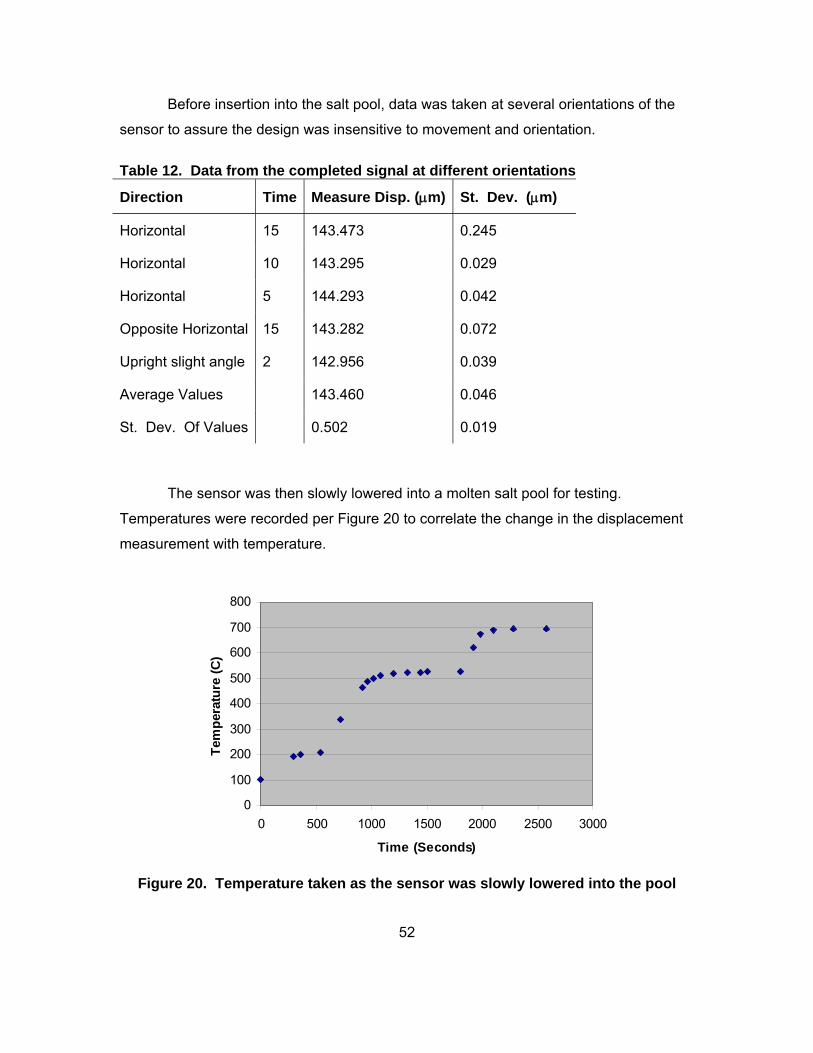
52
Before insertion into the salt pool, data was taken at several orientations of the
sensor to assure the design was insensitive to movement and orientation.
Table 12. Data from the completed signal at different orientations
Direction Time Measure Disp. (m) St. Dev. (m)
Horizontal 15 143.473 0.245
Horizontal 10 143.295 0.029
Horizontal 5 144.293 0.042
Opposite Horizontal 15 143.282 0.072
Upright slight angle 2 142.956 0.039
Average Values 143.460 0.046
St. Dev. Of Values 0.502 0.019
The sensor was then slowly lowered into a molten salt pool for testing.
Temperatures were recorded per Figure 20 to correlate the change in the displacement
measurement with temperature.
0
100
200
300
400
500
600
700
800
0 500 1000 1500 2000 2500 3000
Time (Seconds)
Tem
per
atu
re (
C)
Figure 20. Temperature taken as the sensor was slowly lowered into the pool
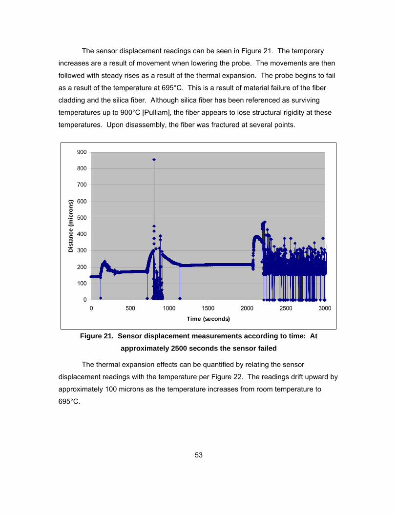
53
The sensor displacement readings can be seen in Figure 21. The temporary
increases are a result of movement when lowering the probe. The movements are then
followed with steady rises as a result of the thermal expansion. The probe begins to fail
as a result of the temperature at 695°C. This is a result of material failure of the fiber
cladding and the silica fiber. Although silica fiber has been referenced as surviving
temperatures up to 900°C [Pulliam], the fiber appears to lose structural rigidity at these
temperatures. Upon disassembly, the fiber was fractured at several points.
0
100
200
300
400
500
600
700
800
900
0 500 1000 1500 2000 2500 3000
Time (seconds)
Dis
tan
ce (
mic
ron
s)
Figure 21. Sensor displacement measurements according to time: At
approximately 2500 seconds the sensor failed
The thermal expansion effects can be quantified by relating the sensor
displacement readings with the temperature per Figure 22. The readings drift upward by
approximately 100 microns as the temperature increases from room temperature to
695°C.
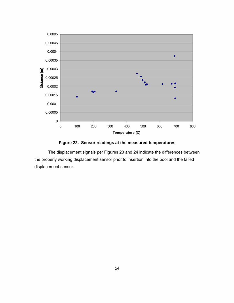
54
0
0.00005
0.0001
0.00015
0.0002
0.00025
0.0003
0.00035
0.0004
0.00045
0.0005
0 100 200 300 400 500 600 700 800
Temperature (C)
Dis
tan
ce (
m)
Figure 22. Sensor readings at the measured temperatures
The displacement signals per Figures 23 and 24 indicate the differences between
the properly working displacement sensor prior to insertion into the pool and the failed
displacement sensor.

55
Figure 23. The sensor image prior to insertion into the pool
Figure 24. The sensor reading after failure.

56
4.6 Modifications
Mature commercial sensors are products of several design cycles. This initial
design cycle brings lessons learned to the next design. An interferometric based fiber
optic pressure sensor provides many benefits in applications to pressure sensing in
harsh environments. Therefore, ORNL and UT continue to investigate custom designed
fiber optic pressure probes addressing lessons learned in the first design cycle.
UT was partnered with ORNL fiber optic experts after the initial design cycle to
investigate optical readout equipment already existing at ORNL. This included a
calibration test for a Thorlabs Si Amplified Detector.
1. Thorlabs Si Amplified Detector: Model PDA 36A; Set at 70 dB
2. TDS5104B Digital Oscilloscope: 1 Mohm impedance
3. Stocker-Yale Fiber Coupled Diode Laser: 634 nm < 5 mW
4. Sensor: Romack Fiber Optics: 040501-003; Two fibers
5. Oriel Model 16121 Micrometer
The calibration curve in Figure 25 indicates the displacement measurement
should occur between the 400 and 500 m where the sensitivity is 5.08 mV/m.
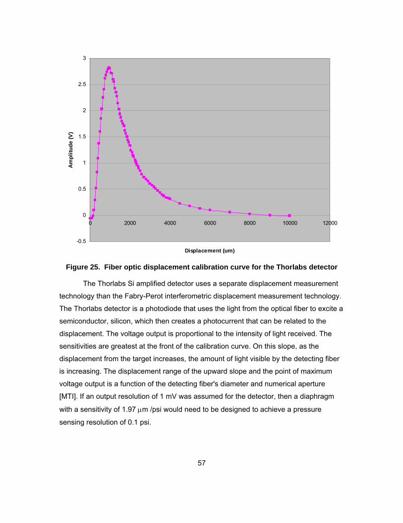
57
-0.5
0
0.5
1
1.5
2
2.5
3
0 2000 4000 6000 8000 10000 12000
Displacement (um)
Am
pli
tud
e (V
)
Figure 25. Fiber optic displacement calibration curve for the Thorlabs detector
The Thorlabs Si amplified detector uses a separate displacement measurement
technology than the Fabry-Perot interferometric displacement measurement technology.
The Thorlabs detector is a photodiode that uses the light from the optical fiber to excite a
semiconductor, silicon, which then creates a photocurrent that can be related to the
displacement. The voltage output is proportional to the intensity of light received. The
sensitivities are greatest at the front of the calibration curve. On this slope, as the
displacement from the target increases, the amount of light visible by the detecting fiber
is increasing. The displacement range of the upward slope and the point of maximum
voltage output is a function of the detecting fiber's diameter and numerical aperture
[MTI]. If an output resolution of 1 mV was assumed for the detector, then a diaphragm
with a sensitivity of 1.97 m /psi would need to be designed to achieve a pressure
sensing resolution of 0.1 psi.
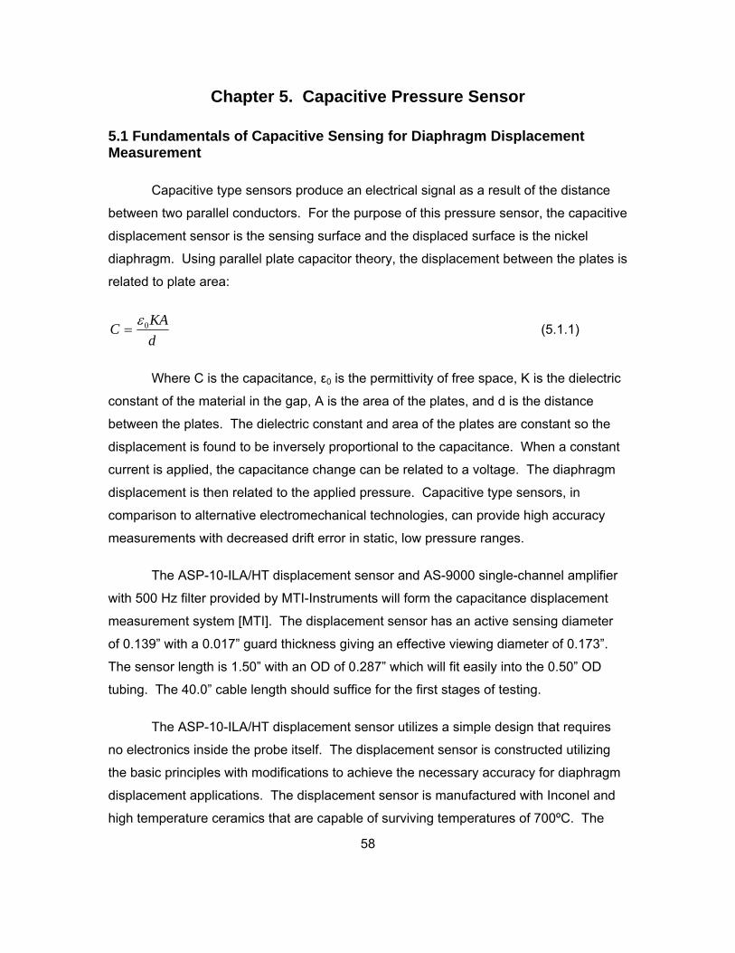
58
Chapter 5. Capacitive Pressure Sensor
5.1 Fundamentals of Capacitive Sensing for Diaphragm Displacement Measurement
Capacitive type sensors produce an electrical signal as a result of the distance
between two parallel conductors. For the purpose of this pressure sensor, the capacitive
displacement sensor is the sensing surface and the displaced surface is the nickel
diaphragm. Using parallel plate capacitor theory, the displacement between the plates is
related to plate area:
d
KAC 0 (5.1.1)
Where C is the capacitance, ε0 is the permittivity of free space, K is the dielectric
constant of the material in the gap, A is the area of the plates, and d is the distance
between the plates. The dielectric constant and area of the plates are constant so the
displacement is found to be inversely proportional to the capacitance. When a constant
current is applied, the capacitance change can be related to a voltage. The diaphragm
displacement is then related to the applied pressure. Capacitive type sensors, in
comparison to alternative electromechanical technologies, can provide high accuracy
measurements with decreased drift error in static, low pressure ranges.
The ASP-10-ILA/HT displacement sensor and AS-9000 single-channel amplifier
with 500 Hz filter provided by MTI-Instruments will form the capacitance displacement
measurement system [MTI]. The displacement sensor has an active sensing diameter
of 0.139” with a 0.017” guard thickness giving an effective viewing diameter of 0.173”.
The sensor length is 1.50” with an OD of 0.287” which will fit easily into the 0.50” OD
tubing. The 40.0” cable length should suffice for the first stages of testing.
The ASP-10-ILA/HT displacement sensor utilizes a simple design that requires
no electronics inside the probe itself. The displacement sensor is constructed utilizing
the basic principles with modifications to achieve the necessary accuracy for diaphragm
displacement applications. The displacement sensor is manufactured with Inconel and
high temperature ceramics that are capable of surviving temperatures of 700ºC. The

59
MTI displacement sensor design shown in Figure 26 has three major elements, the
sensing electrode, guard, and target. To produce accurate results, the electric field
produced between the target and sensing tip must be constant with displacement [MTI],
aligned with the target, and protected from stray capacitance. The guard achieves this
by providing an electric field at the same phase and voltage of the sensing field. The
guard shield is slightly distorted by the ground shield. However, this is acceptable as
long as the sensing field remains linear.
Figure 26. The high temperature capacitive probe provided by MTI
5.2 Bossed Diaphragm
The design of a target for the capacitive displacement sensor requires the use of
a conducting flat diaphragm. This requires a second design for the pressure sensor
housing to accommodate these measurements. The sensing diameter for the capacitive
displacement sensor is 0.173”. The target should be 30% greater than the sensing
diameter to assure linear response. Therefore the sensing diameter should be 0.2249”.
And since this area must be flat, this must be part of the bossed part of the diaphragm.
The current diaphragm diameter is 0.400”. That gives a diameter ratio between the
bossed section and thin section of 0.562 (b/a). Again, nickel was chosen as the material
of choice. However; after later collaboration with ORNL, molybdenum was identified as
a potential diaphragm material with good corrosion resistance and mechanical properties
improved over pure nickel, as shown in Table 13.

60
Table 13. Material properties for diaphragm material selection
Material %Ni %Cr Young’s mod. (GPa)
Poisson’s ratio
Mean Linear Expansion (m/m•°C)
Tensile Strength (MPa)
Yield Strength (MPa)
Ni 200 99 0.00 161 0.28 15.8 125 50.0
Molybdenum - - 292 0.31 161
The deflection at the center of the diaphragm for a flat diaphragm with rigid
bossed center is given as [Di Giovanni]:
)(3
4
0 Eh
PaAy p (5.2.1)
04
3
yaA
EhP
p
(5.2.2)
)log41(16
)1(32
2
4
42
b
a
a
b
a
bAp
(5.2.3)
hyWhere5
1max,0 (5.2.4)
These equations hold true for deflections no more than 20% of the diaphragm’s
thickness.
The maximum stress in the diaphragm is given by:
2 2 2 2max 2 4
3 3( ) ( )
4 2o
p
P Ehya b a b
h A a (5.2.5)
Using the yield stresses above, the minimum thickness for the diaphragm may be found:
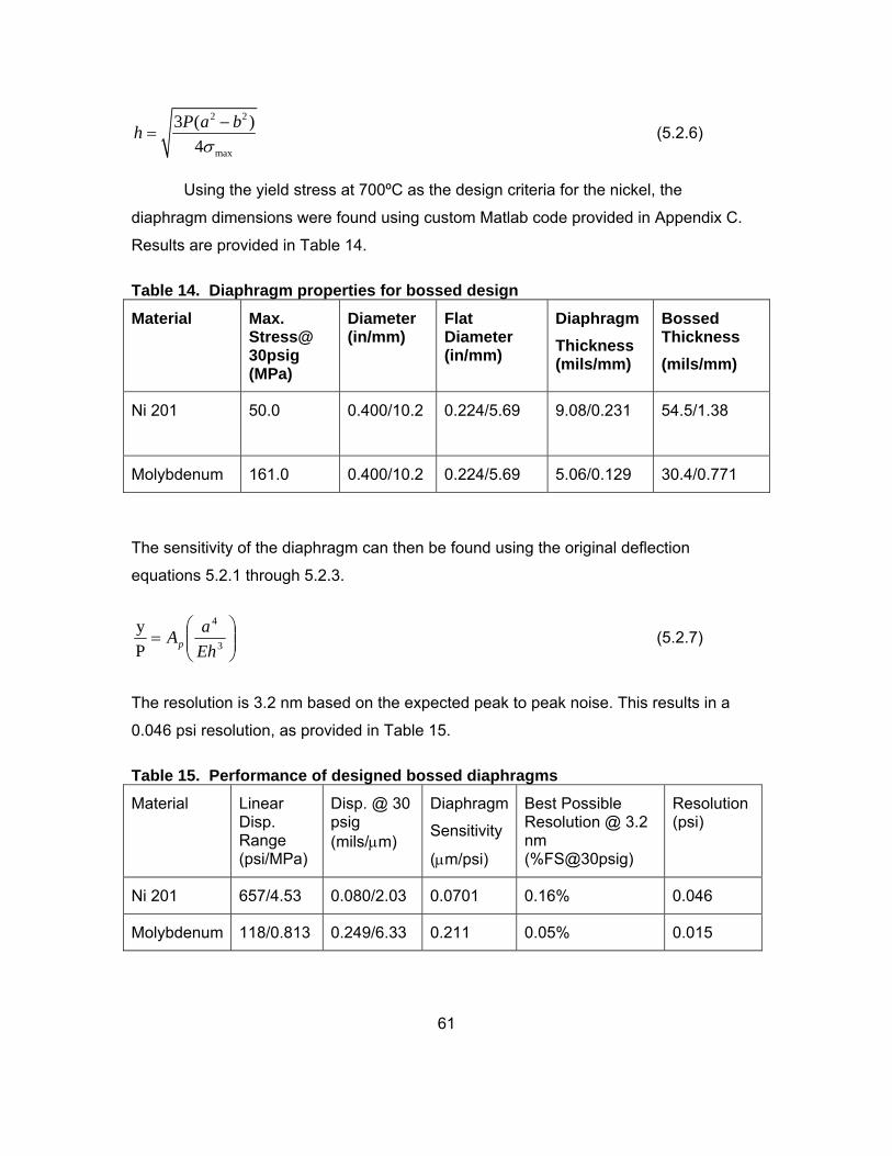
61
2 2
max
3 ( )
4
P a bh
(5.2.6)
Using the yield stress at 700ºC as the design criteria for the nickel, the
diaphragm dimensions were found using custom Matlab code provided in Appendix C.
Results are provided in Table 14.
Table 14. Diaphragm properties for bossed design
Material Max. Stress@ 30psig (MPa)
Diameter (in/mm)
Flat Diameter (in/mm)
Diaphragm
Thickness (mils/mm)
Bossed Thickness
(mils/mm)
Ni 201 50.0
0.400/10.2
0.224/5.69 9.08/0.231 54.5/1.38
Molybdenum 161.0 0.400/10.2 0.224/5.69 5.06/0.129 30.4/0.771
The sensitivity of the diaphragm can then be found using the original deflection
equations 5.2.1 through 5.2.3.
3
4
P
y
Eh
aAp (5.2.7)
The resolution is 3.2 nm based on the expected peak to peak noise. This results in a
0.046 psi resolution, as provided in Table 15.
Table 15. Performance of designed bossed diaphragms
Material Linear Disp. Range (psi/MPa)
Disp. @ 30 psig (mils/m)
Diaphragm
Sensitivity
(m/psi)
Best Possible Resolution @ 3.2 nm (%FS@30psig)
Resolution (psi)
Ni 201 657/4.53 0.080/2.03 0.0701 0.16% 0.046
Molybdenum 118/0.813 0.249/6.33 0.211 0.05% 0.015

62
Figure 27. A half view of the capacitive displacement sensor in position inside the
diaphragm housing (left). The proposed pressure sensor diaphragm for the
capacitive deflection measurement as machined (inches) (right).
Several different configurations were considered. Nickel 200/201 was chosen as
the diaphragm material due to its excellent resistance to corrosion in the high
temperature molten salt environment. The most limiting constraint in the design process
is the yield strength of the diaphragm material at high temperatures. For Nickel, these
values are lower than what other alloys might provide. This leads to lower sensitivity
and potentially smaller diaphragm diameter due to the required support base width.
With Inconel 600 these concerns are eliminated; however, the corrosion depths for
Inconel 600 could potentially cause drift in diaphragm performance and eventual salt
leakage into the sensor cavity. Corrosion depths for Inconel 600 in high temperature
molten salts range from up to 3 mm/year.
When measuring deflections in the sub-nanometer range, it is important to
maintain the dimensional properties of the diaphragm. Too much stress may result in
sensitivity changes and zero-shifts in the pressure sensor due to dimensional distortion.
In order to avoid these problems, it is recommended to keep the maximum stresses in
the diaphragm below the yield strength of the material. A conservative estimate would
place the yield strength for nickel at 18 MPa at 700ºC, much lower than that of Inconel
600. A less conservative estimate would place the yield strength at 50.0 MPa. This less
conservative estimate leads to a larger displacement per unit pressure. In particular, for
63
the test pool, where the pressure will be only a few psig, this less conservative yield
stress estimate will give a design with improved resolution.
5.3 First Design
The pressure sensor consists of 18” long, 0.028” wall thickness, 0.50” O.D.
nickel 200/201 tubing fabricated per details provided in Appendix F. This tubing was
welded to the nickel diaphragm. A small portion of this pressure sensor was subjected
to the full 700ºC environment. To protect the molten salt pool in case of a leak and to
reduce oxidation inside of the probe, an argon gas flowed through the pressure sensor.
The argon should provide very good results as the gap material due to its low dielectric
constant and low variation of dielectric constant with temperature. The capacitive
displacement sensor provided by MTI (model ASP-10-ILA/HT) will be secured inside the
tubing at 50% gap. The original displacement sensor was intended for a 250 m range.
However, since our measurements require only a 2.0 m displacement, the range was
reduced to 125 m. Under this range, 50% gap would be approximately 62.5 m. The
sensitivity is also reduced to12.5 nm/mV. This reduction results in twice the original
resolution. The AS-9000 amplifier was connected to a NI 9215 unit for data acquisition.
The LabView code in Appendix G was then used for displaying the pressure output.
Initial evaluations of the signal accuracy focused on the expected peak to peak
noise to evaluate resolution. For the 500 Hz filter, the manufacturer peak to peak noise
was given as 0.25 mV at 62.5 m. With a predicted 3% sensitivity increase at high
temperatures, the final expected displacement resolution is 3.22 nm. With a total
deflection of 2.03 m at 30 psi, the expected pressure resolution is 0.05 psi.
5.4 Construction and Alignment
Upon receiving the machined material, particularly the cap, probe, and spiders,
the spiders were aligned on the capacitive displacement sensor as indicated in Figures
27 and 28. The spiders are essentially thick washers with set screws. The indentations
are to allow argon to flow through. The two spiders are located on the front end and
back end of the probe such that the probe face is held parallel to the bossed diaphragm
target. The spiders were machined to fit tightly inside the tube to ensure this.
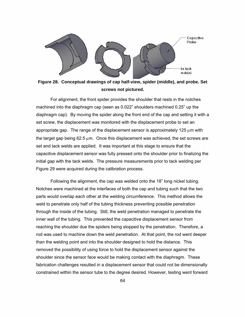
64
Figure 28. Conceptual drawings of cap half-view, spider (middle), and probe. Set
screws not pictured.
For alignment, the front spider provides the shoulder that rests in the notches
machined into the diaphragm cap (seen as 0.022” shoulders machined 0.25” up the
diaphragm cap). By moving the spider along the front end of the cap and setting it with a
set screw, the displacement was monitored with the displacement probe to set an
appropriate gap. The range of the displacement sensor is approximately 125 m with
the target gap being 62.5 m. Once this displacement was achieved, the set screws are
set and tack welds are applied. It was important at this stage to ensure that the
capacitive displacement sensor was fully pressed onto the shoulder prior to finalizing the
initial gap with the tack welds. The pressure measurements prior to tack welding per
Figure 29 were acquired during the calibration process.
Following the alignment, the cap was welded onto the 18” long nickel tubing.
Notches were machined at the interfaces of both the cap and tubing such that the two
parts would overlap each other at the welding circumference. This method allows the
weld to penetrate only half of the tubing thickness preventing possible penetration
through the inside of the tubing. Still, the weld penetration managed to penetrate the
inner wall of the tubing. This prevented the capacitive displacement sensor from
reaching the shoulder due the spiders being stopped by the penetration. Therefore, a
rod was used to machine down the weld penetration. At that point, the rod went deeper
than the welding point and into the shoulder designed to hold the distance. This
removed the possibility of using force to hold the displacement sensor against the
shoulder since the sensor face would be making contact with the diaphragm. These
fabrication challenges resulted in a displacement sensor that could not be dimensionally
constrained within the sensor tube to the degree desired. However, testing went forward

65
since budget and schedule constraints did not provide room for a refabrication of these
parts.
Figure 29. Pressure measurements prior to tack welding.
5.5 High Temperature Testing Apparatus
The pressure sensor was tested per Figure 30 at various pressures using an
argon atmosphere with first tests performed at room temperature, followed by tests
conducted in a high temperature environment. The probe was inserted into a chamber
with argon inlets and outlets for the pressure testing. These were monitored using
standard low pressure gauges. For the high temperature experiments, a small benchtop
furnace (Thermolyne FB1315M) was used. The back of the furnace was removed, and
three holes for the probe and argon tubing were provided.
No tests were performed in the molten salt pool since the nickel 200/201 has
already been proven in the molten salt. Time was also spent attempting to repair an
older furnace for high temperature testing since project hardware funds were expended.
The thermocouples and all four heating elements were damaged, and, after inquiring
about replacement parts, it was determined to be more economical to order a new
furnace.

66
Figure 30. Conceptual drawing of test and completed setup.
During testing, an infrared thermometer was used to monitor temperatures in the
tubing outside the furnace. The temperature dropped significantly only a few inches
outside the furnace. A schematic of components for these evaluations is provided in
Figure 31.
Figure 31. Block diagram of testing setup
5.6 Results
The probe was tested inside the furnace initially at room temperature and
ambient pressure for an extended period. During initial investigations it was found that
the probe was highly susceptible to any disturbance (as little as the door to the lab

67
shutting resulted in a slight drift). This is a result of the displacement sensor not being
firmly seated inside the tube due to the fabiracation challenges.
The data from the initial tests were handled using time averaging and filtering in
Labview. The data were collected at 100 Hz. The filter employed was a lowpass, IIR,
Butterworth filter with 10 Hz cutoff frequency. The time averaging used was
exponentially weighted averaged over 100 ms. Better results are possible by reducing
the filter on the amplifier from 500 Hz to 10 Hz. In Figure 32, analyzing data prior to the
abrupt drift at approximately 500 minutes, the maximum static error for this test was
0.023 psi when tested at atmospheric pressure.
Figure 32. A.) The results of the sensor at ambient conditions. B.) A zoomed view
demonstrating the drift prior to abrupt changes.
The pressure sensor was then calibrated by taking measurements from 0 to 30
psi both upward and downward. Again, the data was manipulated using time averaging
to reduce some random and periodic noise features, thus resulting in slower response
times. Without the averaging, the data has response times limited by the 5 kHz drive
frequency.

68
Figure 33. Calibration data beginning at 30 psi.
Again, as seen in Figure 33, by the end of the testing, the sensor has drifted 3
psi. This drift could be common error such as hysteresis or a physical disturbance.
However, calibration can be used to look at sensitivity, linearity, and hysteresis error.
0
5
10
15
20
25
30
35
40
0 5 10 15 20 25 30 35
Actual Pressure (psi)
Sen
sor
Pre
ssu
re (
psi
)
Down
Up
Drift Corrected Up
Drift Corrected Down
Figure 34. Calibration curve using displayed sensor pressure. This same figure
could feature voltage or displacement as well since it is all linear.
The system was then taken to higher temperatures. The electrical power to
heating coils in the furnace caused the probe to jump sometimes several volts while they

69
were cycling. Once the furnace was finished cycling the probe was able to handle the
high temperatures. However; a Teflon ferrule was being used on the pressure sensor
fitting. Initially this was done to allow flexibility in case the pressure sensor needed to be
altered. However, the Teflon material is not resistant to high temperatures causing a
loss of argon flow. This ended the first phase of testing as the air ingress and high
temperature caused oxidation damage to the diaphragm and fittings. The capacitive
displacement sensor was not well restrained without the structural support provided by
the ferrule used for tube connections. However, some data were obtained for the
pressure sensor at high temperatures.
Figure 35. Results of the probe at 700ºC.
Data taken at 700ºC level out during the last 30 minutes of testing, drifting 2 psi.
With the ferrule sealing the pressure sensor damaged, the relationship between the
actual pressure and measured pressure is not known since the argon was flowing into
the sensor face. The non-averaged data result in a peak to peak noise of 3 mV or 0.6
psi. This is a significant increase over the expected peak-to-peak noise of 0.25 mV.
With filtering and time averaging of data by Labview, the peak to peak resolution in the
pressure signal improves to 0.04 psi.

70
5.7 Modifications
After damaging the ferrule, a sensor rework was undertaken. The tack welds
holding the spider were removed for the addition of a spring loaded housing. New parts
were acquired for this process, and the displacement sensor was recalibrated. Per
Figure 36, the new housing showed an increase in drift, but the drift was stable and
linear.
Figure 36. Spring loaded recalibration data
Following the recalibration, the parts were tack welded. The tack weld
penetrated through the .050” wall and into the guard shell, shorting out the capacitive
sensor. The probe will still perform as long as the outer shell is not conductively
connected to the outer tube and diaphragm. Therefore, a high temperature test can still

71
be planned with this current design if a stable non-conducting holding structure can be
designed.
Another set of modifications are needed to secure the capacitive deflection
measurement sensor in the sensor housing. From initial assessments, the spring loaded
sensor in this design results in a slow, steady drift of the probe closer to the diaphragm.
72
Chapter 8. Conclusions and Recommendations for Future Work
ORNL is assembling a high temperature FliNaK test loop that will utilize induction
heating methods to simulate molten salt flow through a packed pebble bed. The molten
salt test loop will provide necessary flow characteristics and material compatibility testing
for the PB-AHTR design. UT has procured and assembled two pressure sensor designs
using fiber optic and capacitive technologies to measure nickel diaphragm deflections
inside the high temperature molten salt environment. UT has also provided initial flow
loop pressure loss predictions and preliminary air-to-salt heat exchanger design support
for the test loop.
Using preliminary molten salt flow loop designs supplied by ORNL, UT
established methods for predicting flow characteristics through the pebble bed test
section. Two models were used, the Ergun relation and Idelchik resistance coefficients,
to produce flow losses of 0.11 MPa for packing angles of 60º (the maximum amount of
packing). These two outcomes are consistent with the ORNL prediction of 0.1 MPa. UT
also modeled the air-to-salt heat exchanger to remove 100 kW of heat from the system.
All calculations were performed using a custom Matlab code that utilized heat transport
theory and materials from the loop. This code is flexible to provide future assessment of
design changes. The molten salt flow loop was also examined using a fluid transport
code, Fathom 6.0, to analyze flow characteristics in the loop. The code used many of
the same methods featured in the Matlab calculations. The pressure losses in the
pebble bed test section were calculated in Fathom using K-factors taken from the Matlab
calculations. The Fathom code resulted in a pumping power of 318 W at a flow of 4.5
kg/s and a pressure head of 0.143 MPa. These assessments prescribe the pressure
sensing demands for the flow loop that must be provided by the high temperature
pressure sensor developed by UT.
No commercial sensors were available suited to the high temperature and
corrosive salt. The usual method of using an impulse line filled with NaK between the
high temperature diaphragm in contact with the salt and a commercially available low
temperature pressure sensor was not acceptable due to safety and reliability concerns.
73
The pressure sensors designed by UT measure diaphragm displacements to
infer the pressure. The diaphragm design is custom in nickel 200/201, one of few
available materials compatible with FLiNaK salt at 700ºC, and machinable at room
temperature.
The first sensor design utilizes fiber optic technology for the diaphragm
displacement measurement. Fiber optic technology provides great potential for
measurements in harsh environments due to excellent temperature resistance and
insensitivity to electromagnetic interference. The literature indicates that fiber optic
displacement measurements can be made in the sub-nanometer range. Therefore, a
design was developed that utilized Fabry-Perot interferometric technology. The parts for
the pressure sensor housing and diaphragm were procured and assembled by UT. A
laser source and optical readout device was leased from Micron Optics for the Fabry-
Perot measurement. After assembly, the pressure probe was tested at temperatures up
to 700ºC in a molten salt bath at Electrochemical Systems in Oak Ridge, Tennessee.
The pressure sensor was able to give readouts up to 695ºC where the optical fiber and
components failed due to high temperatures. The cladding on the fiber was not able to
withstand the necessary temperatures and the silica fiber was fractured at several
points.
Although fiber optic technology is ideal for the environment of the high
temperature molten salt, the technology is expensive and still in the early stages of
development. Therefore, for the second design, commercially available high
temperature capacitive displacement measurement technology was employed.
Capacitive type sensors have the ability to provide excellent resolution compared to
other displacement measurement methods, making them suitable for small displacement
measurements. The capacitive displacement sensor was provided by MTI Instruments.
The sensor uses high temperature materials and coatings to survive temperatures up to
700ºC. For this design, a flat bossed section on the diaphragm was necessary as a
target for the displacement sensor. A testing apparatus was procured and assembled by
UT that used a modified furnace and argon flow to test the pressure sensor. The
capacitive pressure sensor was tested from 0 to 30 psi at low temperatures, and then
tested again at 700ºC. A loss of the seal around the pressure probe resulted in a loss of
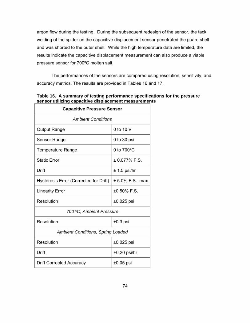
74
argon flow during the testing. During the subsequent redesign of the sensor, the tack
welding of the spider on the capacitive displacement sensor penetrated the guard shell
and was shorted to the outer shell. While the high temperature data are limited, the
results indicate the capacitive displacement measurement can also produce a viable
pressure sensor for 700ºC molten salt.
The performances of the sensors are compared using resolution, sensitivity, and
accuracy metrics. The results are provided in Tables 16 and 17.
Table 16. A summary of testing performance specifications for the pressure sensor utilizing capacitive displacement measurements
Capacitive Pressure Sensor
Ambient Conditions
Output Range 0 to 10 V
Sensor Range 0 to 30 psi
Temperature Range 0 to 700ºC
Static Error ± 0.077% F.S.
Drift ± 1.5 psi/hr
Hysteresis Error (Corrected for Drift) ± 5.0% F.S. max
Linearity Error ±0.50% F.S.
Resolution ±0.025 psi
700 ºC, Ambient Pressure
Resolution ±0.3 psi
Ambient Conditions, Spring Loaded
Resolution ±0.025 psi
Drift +0.20 psi/hr
Drift Corrected Accuracy ±0.05 psi

75
Table 17. A summary of testing performance specifications for the pressure sensor utilizing fiber optic displacement measurements
Fabry Perot Interferometric Probe
Ambient Conditions
Sensor Range 0 to 30 psi
Temperature Range 0 to 695ºC (failed)
Static Error ± 14.38% F.S.
20 to 700 ºC, 2 psi
Temperature Sensitivity +5 psi/ºC
The development of the pressure sensors continues. Future work will build upon
the previous designs to create a reliable high temperature pressure sensor. The fiber
optic sensing technology shows great potential in the field of nuclear power. However,
the optical displacement measurement technology is still developing. Capacitive
displacement measurements provide a well developed technology that is available in
commercial form. However, the capacitive sensor was susceptible to electrical noise
caused by heaters inside the furnace.

76
References
77
References
Berthold, J. W. and Needham, D.B. "Practical Application of Industrial Fiber Optic
Sensing Systems." Davidson Instruments, Inc. n.d. n.p. Web. 1 Oct. 2010.
Bird R.B. et al. Transport Phenomena. New York: John Wiley and Sons, 1960. Print.
Cohen, G. “An Overview of the Concentrating Solar Power Industry: Nevada’s First
Solar Electric Generating System.” Solargenix Energy, Las Vegas, May 2006.
Web. 1 Oct. 2010.
Di Giovanni, M. Flat and Corrugated Diaphragm Design Handbook. New York: Marcel
Dekker, 1982. Print.
Figliola, R.S. and Beasley, D.E. Theory and Design for Mechanical Measurements.
Toronto: John Wiley & Sons, 1991. Print.
Forsberg, C. W. et al., “Molten-Salt-Cooled Advanced High-Temperature Reactor for
Production of Hydrogen and Electricity,” Nuclear Technology, 144, 289–302 ,
2003 . Web. 1 Oct. 2010
Hyun, J.L. and Peterson, P.F. “Conceptual Design of the Intermediate Heat Exchanger
(IHX) for the PB-AHTR.” U.C. Berkeley, May 2009. Web. 1 Oct. 2010.
Idelchik, I.E. Handbook of Hydraulic Resistance. Moscow: Hemisphere Publishing
Company, 1986. 394-396. Print.
Kelly, B. et al. “Nitrate and Nitrate/Nitrite Salt Heat Transport Fluids.” Nexant. Parabolic
Trough Technology Workshop, Colorado 2007, March. Web. 1 Oct. 2010.
Luna Innovations. "Fiber Optic Sensors." Technologies at Luna Innovations, n.d. n.p.
Web. 18 Oct 2010. <http://www.lunainnovations.com/technologies/fiber-
optics.htm>.

78
Mehregany, M. et al. "Silicon Carbide MEMS for Harsh Environments," Proc. of the
IEEE, 1998: 1594-1610. Web 1 Oct. 2010.
MTI-Instruments. "Precision Measurement Instruments." n.d. n.p. Web. 18 Oct 2010.
<http://www.mtiinstruments.com/products/precisioninstruments.aspx>
Murphy, K.A. et al., "Quadrature Phase Shifted Extrinsic Fabry-Perot Optical Fiber
Sensors," Opt. Lett., 16, pp. 273-275, 1991. Web. 1 Oct. 2010.
Murphy, M. "Optical Fiber Pressure Measurement ." Meas. Sci. Technol. 4, 1993: 258-
262. Web. 1 Oct. 2010.
Olson, L. C. "Materials corrosion in molten LiF–NaF–KF salt." Journal of Fluorine
Chemistry 130, 2009: 67-73. Web. 1 Oct. 2010.
Pinet, E. "Fabry-Pérot Fiber-Optic Sensors for Physical Parameters Measurement in
Challenging Conditions ." Journals of Sensors: Fiber and Integrated Waveguide-
Based Optical Sensors. FISO Technologies. Web. 1 Oct. 2010.
Prasanna, S. "Modeling and Characterization of a Fabry Perot Pressure Sensor". The
University of Texas at Arlington, 2005. Web. 1 Oct. 2010
Pulliam, W. and Russler, P. “High-Temperature, High Bandwidth, Fiber-Optic, MEMS
Pressure Sensor Technology for Turbine Engine Component Testing.” Luna
Innovations. Blacksburg, Va. Web. 1 Oct. 2010.
Qi, B. "Novel Data Processing Techniques for Dispersive White Light Interferometer."
Optical Engineering 42, 2003: 3165-3171. Web. 1 Oct. 2010.
Scheeper, P. et al . "The Design, Fabrication, and Testing of Corrugated Silicon Nitride
Diaphragms ." Journal of Microelectromechanical Systems, 1994: 36-42. Web. 1
Oct. 2010
Schulunder, E.U. et al., Heat Exchanger Design Handbook. Washington: Hemisphere
Publishing Corporation, 1982.

79
Shepherd, R. L. and Thacker, L. H. "Evaluation of Pressure Sensor Concepts." Oak
Ridge: ORNL, 1993. Web. 1 Oct. 2010.
Solberg, J. K. "The Influence of Temperature Cycling on the Creep Properties of Nickel
201 and Inconel 600 in Combustion Gas." Journal of Materials Science, 19,
1984: 3908-3924. Web. 1 Oct. 2010.
Special Metals. “Nickel 200 and 201 Properties Sheet.” n.d. n.p. Web. 14, Oct. 2010.
<http://www.specialmetals.com.>
Sporian Microsystems. "High Temperature Sensors." n.d. n.p. Web. 18 Oct 2010.
<http://www.sporian.com/high_temperature_mems.html>.
Udd, E. Fiber Optic Sensors: An Introduction for Engineers and Scientists. New York:
John Wiley & Sons, Inc, 1991. Print.
University of California–Berkeley. "Department of Nuclear Engineering Modular PB-
AHTR System Description." Revision A, April 2009.
University of Wisconsin, Madison et al. “Molten Salt Heat Transport Loop: Materials
Corrosion and Heat Transfer Phenomena.” NERI Final Report., March 2008.
Web. 1 Oct. 2010
Wang, A. et al., "Self-Calibrated Interferometric-Intensity-Based Optical Fiber Sensors,"
J. Lightwave Technol., 19, 2001: 1495-1501. Web. 1 Oct. 2010
Williams, D.F. et al. "Assessment of Candidate Molten Salt Coolants for the Advanced
High-Temperature Reactor (AHTR)." Oak Ridge: UT-Battelle, March 2006. Web.
1 Oct. 2010.
Wilson, J. "Pressure Measurement: Principles and Practice." Journal Weekly Jan. 2003:
n.d. n.p. Web. 18 Oct 2010.
<http://www.sensorsmag.com/sensors/pressure/pressure-measurement-
principles-and-practice-969>.

80
Xu, J. "High Temperature High Bandwidth Fiber Optic Pressure Sensors." Virginia
Polytechnic Institute and State University, Dec. 2005. Web. 1 Oct. 2010.
Yoder, G. et al. “Development of a Forced-Convection Liquid-Fluoride-Salt Test Loop.”
Oct. 2010, Praque. Oak Ridge: ORNL, Proceedings of HTR. Web. 1 Oct. 2010.
Yoder, G. et al., "Analysis of Testing Requirements for Fluoride Salt-Cooled High
Temperature Reactor Components." Oak Ridge: ORNL, 2009. Web. 1 Oct. 2010.
Zhu, F. and Spronck, J. W. "A Simple Capacitive Displacement Sensor." Sensors and
Actuators AI, 25-27, 1991. 265-269. Web. 1 Oct. 2010

81
Appendices

82
Appendix A. Proposed Loop Dimensions
Figure A-1. Proposed Loop Dimensions from early 2009.

83
Table A-1. Loop Functional Requirements
Working fluid FliNaK
Loop maximum operating temperature 700oC
Loop flow rate (to test section) 4.5 kg/s
Test section pressure drop 0.1 MPa
Test section temperature rise 10oC
Loop operating pressure 0.2 Mpa
Pre-heat temperatures 600oC
Heat exchanger 100 kW

84
Appendix B. Matlab Programs for Pressure Drop Calculations
%%%%%%%%%%%%%%%%%%%%%%%%%%%%%%%%%%%%%%%%%%%%%% % %John Ritchie % %Pipe Pressure Drop %%%%%%%%%%%%%%%%%%%%%%%%%%%%%%%%%%%%%%%%%%%%%% clear all; clear; clc; T = input('What is the inlet temperature (Celcius)? '); de = input('What is the pipe diameter(in)? '); Le = input('What is the pipe length(in)? '); m = input('What is the mass flow rate(kg/s)? '); he = input('What is the material roughness (in)?'); ze = input('What is the height change (in)? '); z = ze*0.0254 d = de*0.0254 L = Le*0.0254; h = he*0.0254 A = pi*(d/2)^2; g =9.81; p = -.73*T+2530; mu = 0.04*exp(4170/(T+273.15))*10^-3; V = (m*4)/(p*pi*d^2); Re = (p*V*d)/mu relative_roughness = h/d f = input('What is the friction factor from the moody chart? '); %Minor Losses i = input('Is there a bend (1 for yes, 0 for no)?'); j = input('Is there a sudden contraction (1 for yes, 0 for no)?'); k = input('Is there a sudden expansion (1 for yes, 0 for no)?'); if i==1; K1 = 0.25; end if i==0; K1=0; end if j==1; F1 = input('What is the cross-section area of the larger area?'); K2 = 0.5*(1-(A/F1)); end
85
if j==0; K2=0; end if k==1; F1 = input('What is the cross-section area of the larger area?'); K3 = (1-(A/F1))^2; end if k==0; K3=0; end K= K1+K2+K3 %PD calculation PD = p*g*(z)+.5*p*V^2*f*(L/d)+K*p*V^2*.5 %%%%%%%%%%%%%%%%%%%%%%%%%%%%%%%%%%%%%%%%%%%%%% % %John Ritchie % %Test Section Pressure Drop %%%%%%%%%%%%%%%%%%%%%%%%%%%%%%%%%%%%%%%%%%%%%% clear all; clear; clc; Ti = input('What is the inlet temperature (Celcius)? '); To = input('What is the outlet temperature (Celcius)? '); de = input('What is the Test Section diameter(in)? '); Le = input('What is the T.S. length(in)? '); m= input('What is the inlet mass flow rate(kg/s)? '); dpe = input('What is the pellet diameter(cm)?'); thd = input('What is the pellet packing angle(degrees) (60-90)?'); th = thd*pi/180; d = de*0.0254; L = Le*0.0254; dp = dpe*0.01; po = -.73*To+2530; pin = -.73*Ti+2530; pm = -.73*Ti+2530; Tm = (Ti+To)/2; g = 9.81; A = pi*(d/2)^2; Vi = m/(pin*A); Vo = m/(A*po); Vavg = (Vi+Vo)/2; mui = 0.04*exp(4170/(Ti+273.15))*10^-3; muo = 0.04*exp(4170/(To+273.15))*10^-3; mum = 0.04*exp(4170/(Tm+273.15))*10^-3;
86
ei= 1-(pi/(6*(1-cos(th))*sqrt(1+2*cos(th)))); Rem = ((0.45)/((1-ei)*sqrt(ei)))*pm*Vavg*dp/mum E = (1.53/ei^(4.2))*((30/Rem)+(3/Rem^0.7)+0.3)*(L/dp); PD = E*pm*(Vavg^2)*0.5 + pin*Vi*(Vo-Vi)+pm*g*L %%%%%%%%%%%%%%%%%%%%%%%%%%%%%%%%%%%%%%%%%%%%%% % %John Ritchie % %Heat Exchanger Pressure Drop %%%%%%%%%%%%%%%%%%%%%%%%%%%%%%%%%%%%%%%%%%%%%% clear all; clear; clc; % Ti = input('What is the inlet temperature (Celcius)? '); % To = input('What is the outlet temperature (Celcius)? '); % Tai = input('What is room temperature (Celcius)? '); % n = input('How many tubes? '); % Le = input('What is the HX length(in)? '); % m= input('What is the inlet mass flow rate(kg/s)? '); Ti = 700; Tai = 20+273; n =1; Le = 52; % we=30; mi=4.5; U=138; Tao = 65+273; Qi = 100000; xe = .25; t = .001; %Constants and unit conversion Q= Qi/n m = mi/n L = Le*0.0254; g = 9.81; x = xe*0.0254; k = 0.92; Cp = 1.886E3; To = -Q/(m*Cp)+Ti; %Thermophysical properties of molten salt Tm = (Ti+To)/2; po = -.73*To+2530; pin = -.73*Ti+2530; pm = -.73*Ti+2530;

87
mui = 0.04*exp(4170/(Ti+273.15))*10^-3; muo = 0.04*exp(4170/(To+273.15))*10^-3; mum = 0.04*exp(4170/(Tm+273.15))*10^-3; %Thermophysical properties of air (inlet) Cpi = (-1.900540E-10*Tai^3 + 5.067580E-7*Tai^2-2.101781E-4*Tai + 1.034189)*10^3; muai =(1.626263E-7*Tai^3 - 4.670448E-4*Tai^2+7.256015E-1*Tai +4.167699)*10^(-7); pai = 355.31*Tai^(-1.0029); ma = Q/(Cpi*(Tao-Tai)); %Thermophysical properties of air (outlet and mean) Tam = (Tao+Tai)/2; Cpo= (-1.900540E-10*Tao^3 + 5.067580E-7*Tao^2-2.101781E-4*Tao + 1.034189)*10^3; Cpm = (-1.900540E-10*Tam^3 + 5.067580E-7*Tam^2-2.101781E-4*Tam + 1.034189)*10^3; pao = 355.31*Tao^(-1.0029); pam = 355.31*Tam^(-1.0029); muao = (1.626263E-7*Tao^3 - 4.670448E-4*Tao^2+7.256015E-1*Tao +4.167699)*10^(-7); muam = (1.626263E-7*Tam^3 - 4.670448E-4*Tam^2+7.256015E-1*Tam +4.167699)*10^(-7); %what is volumetric flow rate needed from the fan? V = ma/pam; Cr = (Cpm*ma)/(Cp*m) P = (Ti-To)/(Ti+273.15-Tai) NTU = input('What is the NTU value? '); A1 = (NTU*Cpm*ma)/U; %h for internal flow w = A1/(2*L); Ax = w*x; d = 4*(w*x)/(2*w+2*x); Vi = m/(pin*Ax); Vo = m/(Ax*po); Vavg = (Vi+Vo)/2; Rem = (pm*Vavg*d)/mum; Rei = (pin*Vi*d)/mui; Reo = (po*Vo*d)/muo; Pr = (Cp*mum)/k; Nu = 0.023*Rem^0.8*Pr^0.3; h1 = (k*Nu)/d;
88
%h for external flow kam = (3.359175E-8*Tam^3-8.703488E-5*Tam^2+1.230714E-1*Tam -3.116276)*10^(-3); A2 = 2*(w+2*t)*L; Axa = L*(x+2*t); Ream = (pam*(ma/(Axa*pam))*w)/muam; Prm = Cpm*muam/kam; Nua = (0.037*Ream^0.8*Prm)/(1+2.443*Ream^(-0.1)*(Prm^(2/3)-1)); h2 = Nua*kam/L; %Find the actual U U1 = (1/A1)/((1/(h1*A1))+(1E-4/A1)+(t/(23.6*w*L))+(0.0004/A2)+(1/(h2*A2))) UA= (A1)*U1; UAe = Q/((Ti+273)-Tai); Qi = UA*(Tavg+273.15-Tai); Q=Qi*n Y= abs((U-U1)/(U)); %Tube Pressure Drop disp(Rem) hf = 1E-7*0.0254; relative_roughness = hf/d f = input('What is the friction factor from the moody chart? '); F1= (w*n*x)/n; PD1 = n*(f*(L/d)+(0.5*(1-(Ax/F1)))+((1-(Ax/F1))^2))*pm*(Vavg^2)*0.5 + pin*Vi*(Vo-Vi)-pm*g*L %%%%%%%%%%%%%%%%%%%%%%%%%%%%%%%%%%%%%%%%%%%%%% % %John Ritchie % %Heat Exchanger Pressure Drop %%%%%%%%%%%%%%%%%%%%%%%%%%%%%%%%%%%%%%%%%%%%%% clear all; clear; clc; % Ti = input('What is the inlet temperature (Celcius)? '); % To = input('What is the outlet temperature (Celcius)? '); % Tai = input('What is room temperature (Celcius)? '); % n = input('How many tubes? '); % Le = input('What is the HX length(in)? '); % w = input('What is the HX width (in)?') % m= input('What is the inlet mass flow rate(kg/s)? ');

89
Ti = 700; Tai = 20+273; n =30; Le = 52; mi=4.5; we = 7.9; Tao = 65+273; Qi = 100000; xe = .25; t = .001; %Constants and unit conversion Q= Qi/n m = mi/n L = Le*0.0254; g = 9.81; w= we*0.0254 x = xe*0.0254; k = 0.92; Cp = 1.886E3; To = -Q/(m*Cp)+Ti; A1=2*w*L %Thermophysical properties of molten salt Tm = (Ti+To)/2; po = -.73*To+2530; pin = -.73*Ti+2530; pm = -.73*Ti+2530; mui = 0.04*exp(4170/(Ti+273.15))*10^-3; muo = 0.04*exp(4170/(To+273.15))*10^-3; mum = 0.04*exp(4170/(Tm+273.15))*10^-3; %Thermophysical properties of air (inlet) Cpi = (-1.900540E-10*Tai^3 + 5.067580E-7*Tai^2-2.101781E-4*Tai + 1.034189)*10^3; muai =(1.626263E-7*Tai^3 - 4.670448E-4*Tai^2+7.256015E-1*Tai +4.167699)*10^(-7); pai = 355.31*Tai^(-1.0029); mai = Q/(Cpi*(Tao-Tai)); ma = mai %Thermophysical properties of air (outlet and mean) Tam = (Tao+Tai)/2; Cpo= (-1.900540E-10*Tao^3 + 5.067580E-7*Tao^2-2.101781E-4*Tao + 1.034189)*10^3; Cpm = (-1.900540E-10*Tam^3 + 5.067580E-7*Tam^2-2.101781E-4*Tam + 1.034189)*10^3; pao = 355.31*Tao^(-1.0029); pam = 355.31*Tam^(-1.0029); muao = (1.626263E-7*Tao^3 - 4.670448E-4*Tao^2+7.256015E-1*Tao +4.167699)*10^(-7); muam = (1.626263E-7*Tam^3 - 4.670448E-4*Tam^2+7.256015E-1*Tam +4.167699)*10^(-7);
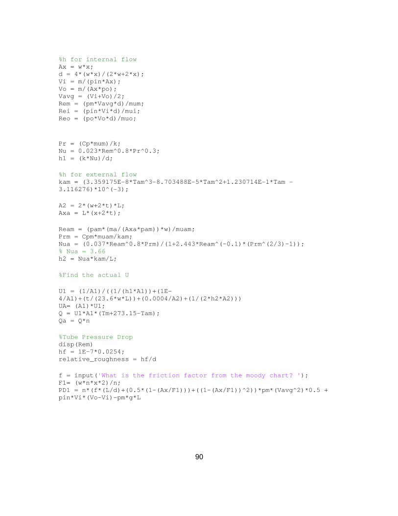
90
%h for internal flow Ax = w*x; d = 4*(w*x)/(2*w+2*x); Vi = m/(pin*Ax); Vo = m/(Ax*po); Vavg = (Vi+Vo)/2; Rem = (pm*Vavg*d)/mum; Rei = (pin*Vi*d)/mui; Reo = (po*Vo*d)/muo; Pr = (Cp*mum)/k; Nu = 0.023*Rem^0.8*Pr^0.3; h1 = (k*Nu)/d; %h for external flow kam = (3.359175E-8*Tam^3-8.703488E-5*Tam^2+1.230714E-1*Tam -3.116276)*10^(-3); A2 = 2*(w+2*t)*L; Axa = L*(x+2*t); Ream = (pam*(ma/(Axa*pam))*w)/muam; Prm = Cpm*muam/kam; Nua = (0.037*Ream^0.8*Prm)/(1+2.443*Ream^(-0.1)*(Prm^(2/3)-1)); % Nua = 3.66 h2 = Nua*kam/L; %Find the actual U U1 = (1/A1)/((1/(h1*A1))+(1E-4/A1)+(t/(23.6*w*L))+(0.0004/A2)+(1/(2*h2*A2))) UA= (A1)*U1; Q = U1*A1*(Tm+273.15-Tam); Qa = Q*n %Tube Pressure Drop disp(Rem) hf = 1E-7*0.0254; relative_roughness = hf/d f = input('What is the friction factor from the moody chart? '); F1= (w*n*x*2)/n; PD1 = n*(f*(L/d)+(0.5*(1-(Ax/F1)))+((1-(Ax/F1))^2))*pm*(Vavg^2)*0.5 + pin*Vi*(Vo-Vi)-pm*g*L

91
Appendix C. Matlab Code for Diaphragm Design (Bossed)
% %John Ritchie % %Flat Diaphragm Design %%%%%%%%%%%%%%%%%%%%%%%%%%%%%%%%%%%%%%%%%%%%%% clear all; clear; clc; clf; E = 161E9; mu = 0.28; P =206*10^3; sig = 18E6 %Thickness calculation de = .4; d = de*2.54*.01; t = (0.75*(P*(d/2)^2)/(sig))^0.5; te = t*100/2.54; wlmax = 0.2*te; w0 = (3*(1-mu^2)*P*d)/(16*E*t^3); w0e = w0*100/2.54; a = d/2; Y = (3*(1-mu^2)*a^4)/(16*E*t^3); %Deflection Profile x = 0:.0001:a; x2 = x./a; y = [1-((x./a).^2)].^2; figure(1) plot(x2,y) xlabel('Radial Distance (r/a)'); ylabel('Deflection (y/y0)'); figure(2) x3=0:200; x3 = x3*10^-6; P2 = (16*E*t^4.*x3)/(3*(1-mu^2)*t*a^4); P3 = (16*E*t^4.*x3)/(3*(1-mu^2)*t*a^4)+((7-mu)*x3.^3*E*t^4)/(3*(1-mu)*t^3*a^4); x3 = x3*10^6; P2 = P2*10^-6; P3 = P3*10^-6; figure(2) plot(x3,P2,'g',x3,P3,'-.r') xlabel('Displacement (microns)'); ylabel('Pressure (MPa)'); legend('Linear', 'Actual') %Stresses P5 = 0.2E6 Sr= (3/8)*P5*a^2/t^2*((3+mu)*x.^2/a^2-(1+mu)); St = (3/8)*P5*a^2/t^2*((3*mu+1)*x.^2/a^2-(1+mu));

92
figure(3) plot(x2,Sr,x2,St) xlabel('Radial Distance (r/a)'); ylabel('Stress(Pa)'); legend('Radial', 'Tangential') %%%%%%%%%%%%%%%%%%%%%%%%%%%%%%%%%%%%%%%%%%%%%% % %John Ritchie % %Bossed Diaphragm Design %%%%%%%%%%%%%%%%%%%%%%%%%%%%%%%%%%%%%%%%%%%%%% clear all; clear; clc; clf; % Input Variables E = 292.45E9; %Young's Modulus mu = 0.31; %Poisson's Ratio P=0.2E6; %Actual Pressure (Pa) sig = 160.66E6 % 2% Yield Stress (Pa) de = 0.40; %Diaphragm Diameter (in.) Pe = P/6894 %Pressure in psi % Variable Calculation d = de*2.54*.01; a = d/2; b = 5.69*10^-3/2; bovera = b/a de_flat = b*200/2.54; %Bossed Diameter d_flat = b*2; % Thickness Calculation Ap = (3*(1-mu^2)/16)*(1-(b^4/a^4)-4*(b^2/a^2)*log(a/b)); h = ((5*Ap*P*a^4)/E)^(1/4); he = h*100/2.54; y= (Ap*P*a^4)/(E*h^3); %Deflection at Max Pressure (m) ye = y*100/2.54; % Measurables yOVERh=y/h; %Ratio of max deflection to thickness, must be less than 0.2 Y = y/P; %Sensitivity (m/Pa) Ye = Y*10^6*6894 %Linear Deflection Plot P2 = 0:.01:0.2; y02= (Ap*P2*10^6*a^4)/(E*h^3)*10^6; figure(1) plot(P2,y02)
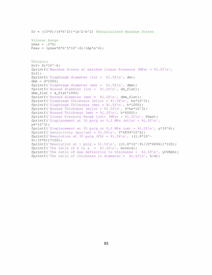
93
Sr = ((3*P)/(4*h^2))*(a^2-b^2) %Recalculated Maximum Stress %Linear Range ymax = .2*h; Pmax = (ymax*E*h^3*10^-6)/(Ap*a^4); %Outputs Sr2= Sr*10^-6; fprintf('Maximum Stress at maximum linear Pressure (MPa) = %1.5f\n', Sr2); fprintf('Diaphragm diameter (in) = %1.5f\n', de); dmm = d*1000; fprintf('Diaphragm diameter (mm) = %1.5f\n', dmm); fprintf('Bossed diameter (in) = %1.5f\n', de_flat); dmm_flat = d_flat*1000; fprintf('Bossed diameter (mm) = %1.5f\n', dmm_flat); fprintf('Diaphragm Thickness (mils) = %1.5f\n', he*10^3); fprintf('Diaphragm Thickness (mm) = %1.5f\n', h*1000); fprintf('Bossed Thickness (mils) = %1.5f\n', 6*he*10^3); fprintf('Bossed Thickness (mm) = %1.5f\n', h*6000); fprintf('Linear Pressure Range Limit (MPa) = %1.5f\n', Pmax); fprintf('Displacement at 30 psig or 0.2 MPa (mils) = %1.5f\n', ye*10^3); fprintf('Displacement at 30 psig or 0.2 MPa (um) = %1.5f\n', y*10^6); fprintf('Sensitivity (psi/um) = %1.5f\n', Y*6894*10^6); fprintf('Resolution at 30 psig (FS) = %1.5f\n', ((1.8*10^-9)/(Y*P))*100); fprintf('Resolution at 1 psig = %1.5f\n', ((1.8*10^-9)/(Y*6894))*100); fprintf('The ratio of b to a = %1.5f\n', bovera); fprintf('The ratio of max deflection to thickness = %1.5f\n', yOVERh); fprintf('The ratio of thickness to diameter = %1.5f\n', h/d);

94
Appendix D. Machining Proposal for Fiber Optic Probe
Proposed Fiber Optic Pressure Sensor for the Molten Salt Pool
Date: September 14, 2009
*All units in inches
Background:
A fiber optic pressure sensor is being developed for a molten salt very high temperature
environment (700°C). The sensor will be placed in a molten salt bath through a 0.50”
tube. This proposal is asking for:
Process Flow
The following components are to be machined out of the following materials supplied by
UTK. The machined components will then be sent to ORNL for laser tack welding where
specified. The machined components will be examined or machined to specifications
post-welding. Circumferential arc welding to be performed on the end-cap and outer
0.500” OD x 0.028” wall tubing. The completed machining and welding will include two
final components:
The outer 18” long x 0.028” wall tubing arc welded to an end cap that houses a
nickel spacer tack welded to the end-cap.
The inner 18” long x 0.028” wall tubing tack welded to the nickel-fiber housing
This design will allow for easy removal or insertion of the inner tubing into the outer
tubing while maintaining an air cavity which constitutes the deflection to be measured.
All tolerances related to this cavity height are important in maintaining the measurement
integrity. A thermocouple and optical fiber will run through the nickel-fiber housing. A
separate hole will be drilled to allow for close to atmospheric pressure in the cavity. A
completed drawing of this proposed sensor can be seen at the conclusion of this
document.

95
I. Diaphragm/End-Cap:
Material: Nickel 201
Figure D-1. Nickel 201 diaphragm.
Tolerances for bored-through lengths +/- 0.0005” due to cavity height (0.0815” +/-
0.0005”). All other tolerances +/- 0.005. Nickel 201 0.50” bar will be provided.
Figure D-2. Conceptual drawing showing the diaphragm and shelf for the nickel
spacer.
Nickel 201 Bar provider: Corrosion Materials: Nickel 200/201 1/2 IN, 5 FT Round Bar,
3.84 LB, Cost: $109.23.
Nickel Spacer: Material: Nickel 201
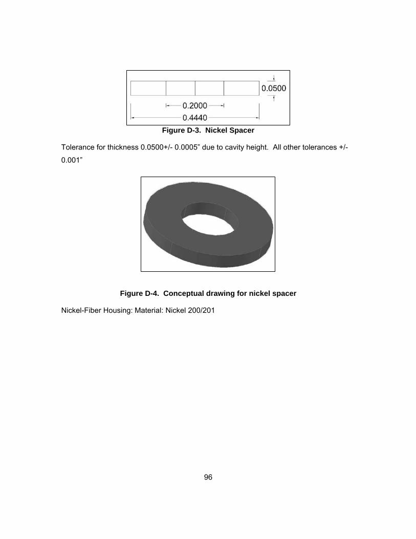
96
Figure D-3. Nickel Spacer
Tolerance for thickness 0.0500+/- 0.0005” due to cavity height. All other tolerances +/-
0.001”
Figure D-4. Conceptual drawing for nickel spacer
Nickel-Fiber Housing: Material: Nickel 200/201

97
Figure D-5. Nickel-Fiber Housing
The housing is to be machined from a single piece of 0.50” Nickel 201 bar (same as
diaphragm). This piece will be laser tack welded by ORNL to the 18” long, 0.25” inner
tubing.
Drilled insert for optical fiber
Drilled insert for thermocouple (d=0.03”)
Drilled hole for air flow (d=0.03”)
Tolerance for smaller section thickness +/- 0.0005” due to cavity height (0.1299” +/-
0.0005”)
The tip of the insert for the fiber optic holder should be 0.01” to hold optical fiber in
alignment. The rest of the insert can be drilled to machinist’s preference as it is not of
importance. All other dimensions to the machinist’s preference (i.e. chamfer and top
diameter).
Tolerances for diameters +/- 0.005. All other tolerances +/- 0.01”

98
Figure D-6. Conceptual drawing showing the nickel-fiber housing.
Outer Tubing:
Material: Nickel 200
Outer Diameter: 0.500”
Inner Diameter: 0.4334”
Thickness: 0.028” (or available)
Length: 18”
Provider: Eagle Alloys
Nickel alloy 200 seamless tube
20 ft.min. 1/2"od x .028"w x 20'
$38.25/ft; $765.00 min.
Inner Tubing:
Material: Nickel 200
Outer Diameter: 0.2500”
Inner Diameter: 0.2220” (or available)
Thickness: 0.0280” (or available)

99
Length: 18.0”
Provider: MicroGroup
Nickel 200
Tubular Materials; Round / Hypo; 200 Fractional .250" OD x .028" Wall x Seamless; OD
min/max: 0.2450/0.2550; ID min/max: 0.1806/0.2074; Wall min/max: 0.0238/0.0322; 5
pcs @ 18 inches; +/-0.06" tolerance
Cost: $83.31/pc
Figure D-7. Dimensions of tubing (actual length 18”) and top of inner 0.25”
diameter tubing
Overview/Completed Sensor Head:
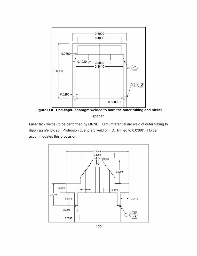
100
Figure D-8. End-cap/Diaphragm welded to both the outer tubing and nickel
spacer.
Laser tack welds (to be performed by ORNL). Circumferential arc weld of outer tubing to
diaphragm/end-cap. Protrusion due to arc weld on I.D. limited to 0.0300”. Holder
accommodates this protrusion.

101
Figure D-9. Nickel-fiber housing welded to inner tubing.
Figure D-10. Overview of sensor head with all components as specified.
1. Laser tack welds (to be performed by ORNL)
2. Circumferential arc weld of outer tubing to diaphragm/end-cap
3. The priority dimension is the spacing between the fiber tip and
diaphragm which should be approximately 0.0016”. The fiber holder will slide into and
out of the washer where it sits. Therefore, the dimensions (0.1315” and 0.1299”) can be
machined as long as the difference remains at 0.0016”.
4. 0.0050” spacing between fiber housing and nickel spacer such
that the holder slides somewhat easily into place upon removal or insertion.
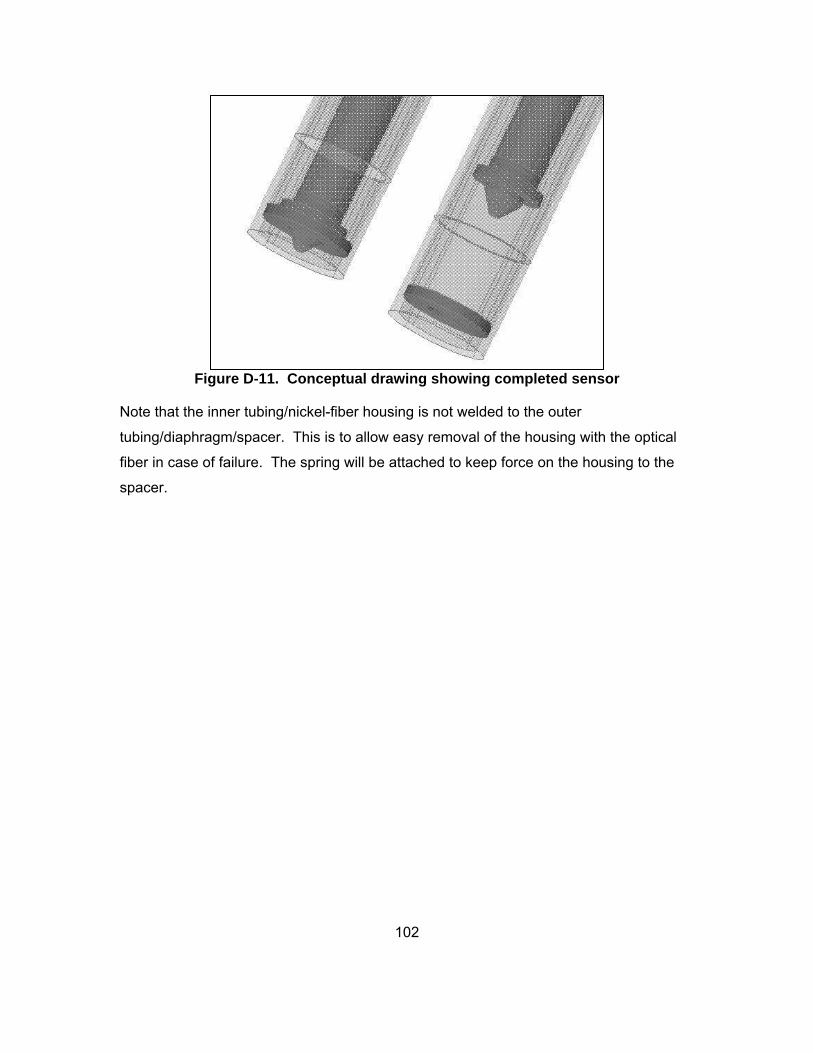
102
Figure D-11. Conceptual drawing showing completed sensor
Note that the inner tubing/nickel-fiber housing is not welded to the outer
tubing/diaphragm/spacer. This is to allow easy removal of the housing with the optical
fiber in case of failure. The spring will be attached to keep force on the housing to the
spacer.

103
Appendix E. Labview Code for Fiber Optic Pressure Probe
Figure E-1. Labview block diagram for fiber optic pressure measurements
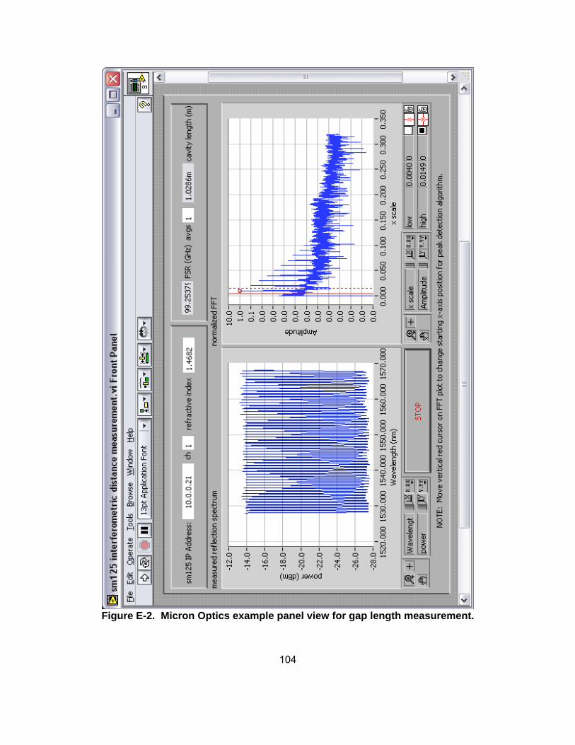
104
Figure E-2. Micron Optics example panel view for gap length measurement.
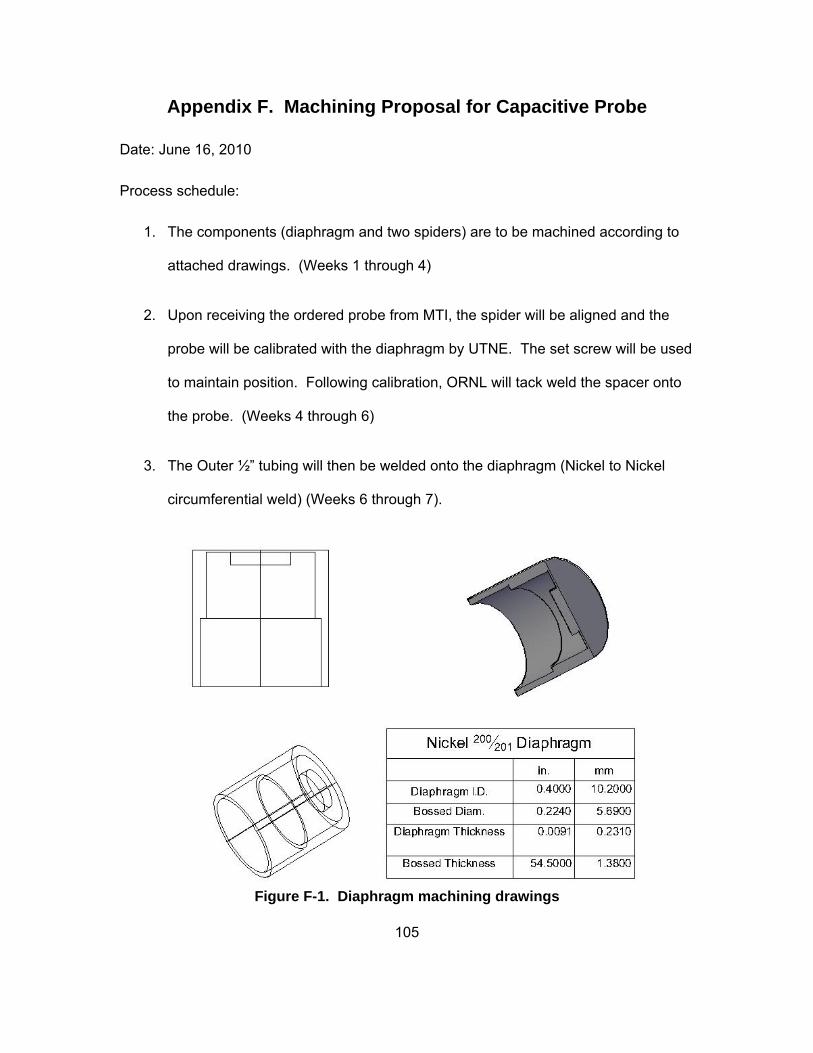
105
Appendix F. Machining Proposal for Capacitive Probe
Date: June 16, 2010
Process schedule:
1. The components (diaphragm and two spiders) are to be machined according to
attached drawings. (Weeks 1 through 4)
2. Upon receiving the ordered probe from MTI, the spider will be aligned and the
probe will be calibrated with the diaphragm by UTNE. The set screw will be used
to maintain position. Following calibration, ORNL will tack weld the spacer onto
the probe. (Weeks 4 through 6)
3. The Outer ½” tubing will then be welded onto the diaphragm (Nickel to Nickel
circumferential weld) (Weeks 6 through 7).
Figure F-1. Diaphragm machining drawings
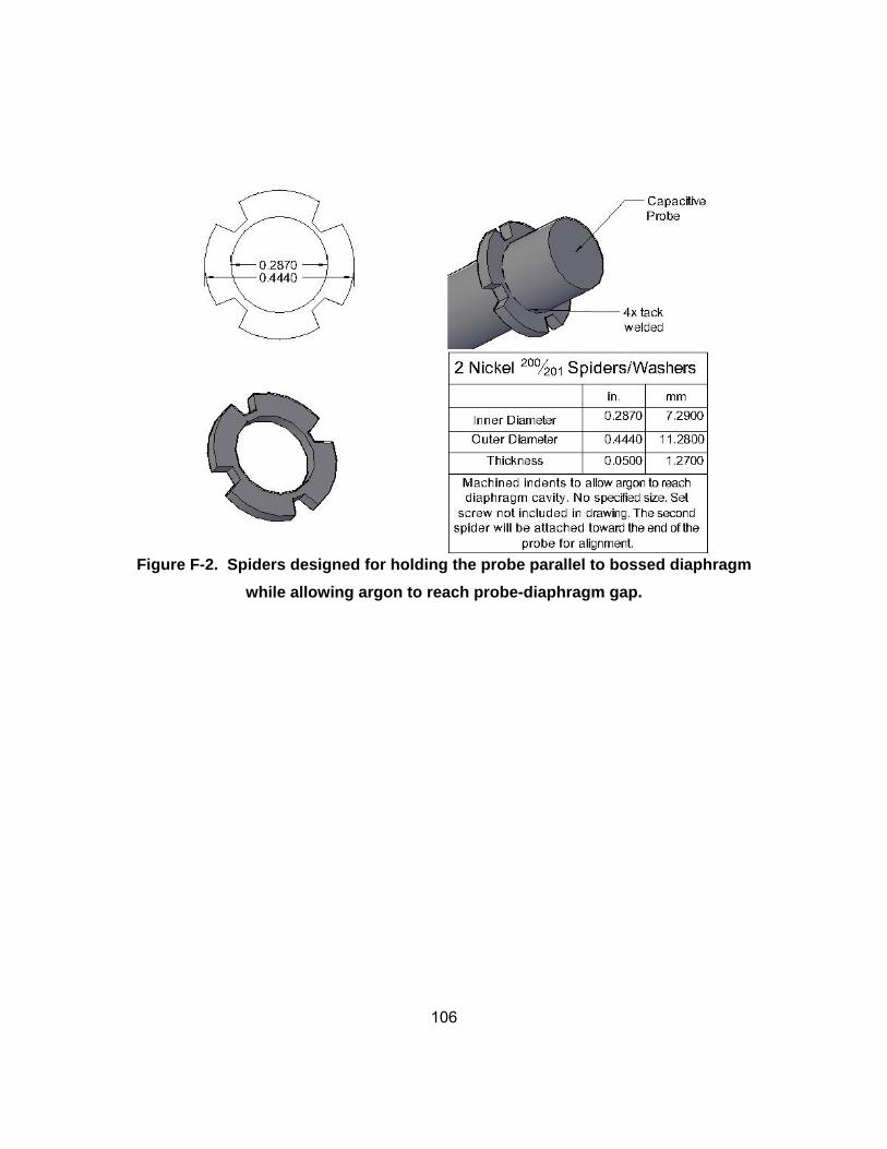
106
Figure F-2. Spiders designed for holding the probe parallel to bossed diaphragm
while allowing argon to reach probe-diaphragm gap.
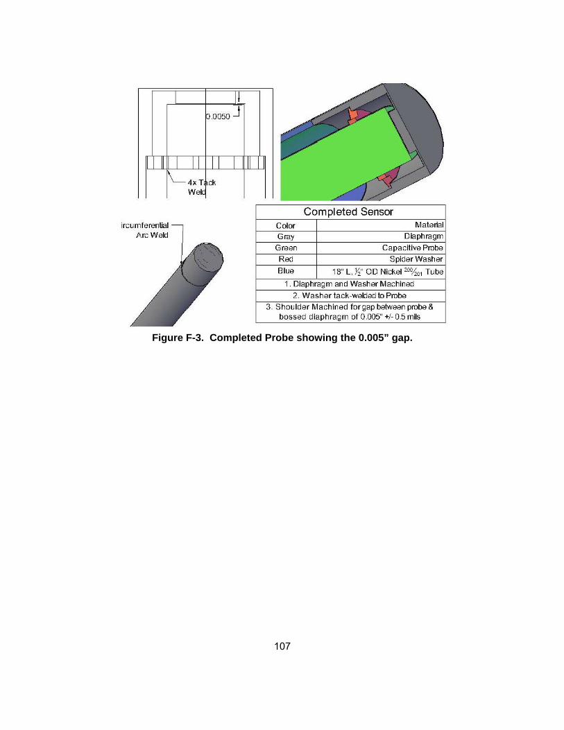
107
Figure F-3. Completed Probe showing the 0.005” gap.
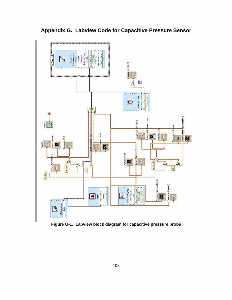
108
Appendix G. Labview Code for Capacitive Pressure Sensor
Figure G-1. Labview block diagram for capacitive pressure probe
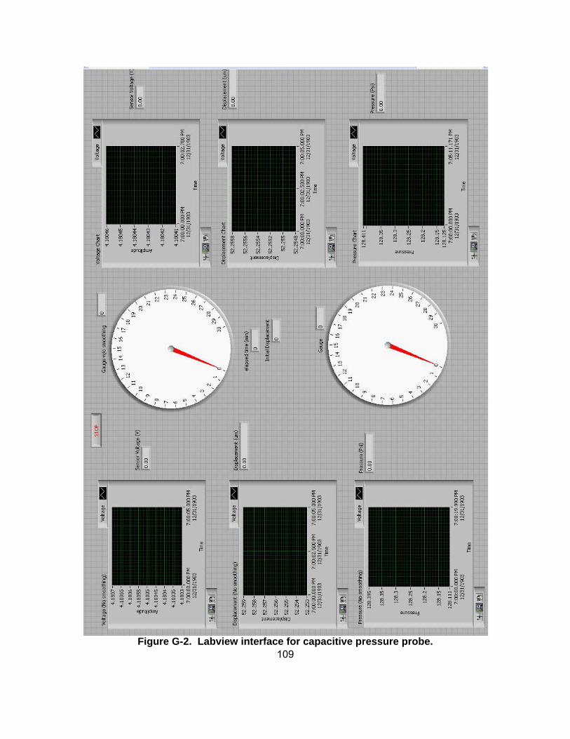
109
Figure G-2. Labview interface for capacitive pressure probe.

110
Vita
John Andrew Ritchie was born on November 22, 1986 in Chattanooga,
Tennessee to the parents of Johnny and Deborah Ritchie. He is the last of three sons:
Joseph and Adam Ritchie. After graduating from Hixson High School, he decided to
attend the University of Tennessee-Knoxville. Inspired by his father, an employee at the
Tennessee Valley Authority for more than 30 years, John decided to follow a path in
Nuclear Engineering. Upon enrolling at UTK, John was accepted into the UTK
Chancellor’s Honors Program in which he maintained membership throughout his
college tenure. While at UT, John participated in a TVA internship at Watts Bar Nuclear
Power Plant in the summer of 2008. Following the internship, he began working as an
undergraduate research assistant at the university. In May of 2009, John obtained his
Bachelor’s of Science in Nuclear Engineering graduating Magna Cum Laude. Following
undergraduate graduation, John began his work at the University of Tennessee-
Knoxville Graduate School in Nuclear Engineering.