prettynu multi-dependent criteria supplier selection …
TRANSCRIPT
prettynu
MULTI-DEPENDENT CRITERIA SUPPLIER SELECTION
WITH UNCERTAIN PERFORMANCE EVALUATION
Miss Ornicha Anuchitchanchai
A Dissertation Submitted in Partial Fulfillment of the Requirements
for the Degree of Doctor of Philosophy Program in Logistics Management
(Interdisciplinary Program)
Graduate School
Chulalongkorn University
Academic Year 2017
Copyright of Chulalongkorn University

การคดเลอกผสงมอบแบบหลายเกณฑโดยการประเมนความไมแนนอนของผลการด าเนนงาน
นางสาวอรณชา อนชตชาญชย
วทยานพนธนเปนสวนหนงของการศกษาตามหลกสตรปรญญาวทยาศาสตรดษฎบณฑต
สาขาวชาการจดการดานโลจสตกส (สหสาขาวชา)
บณฑตวทยาลย จฬาลงกรณมหาวทยาลย
ปการศกษา 2560
ลขสทธของจฬาลงกรณมหาวทยาลย
Thesis Title MULTI-DEPENDENT CRITERIA SUPPLIER
SELECTION WITH UNCERTAIN
PERFORMANCE EVALUATION
By Miss Ornicha Anuchitchanchai
Field of Study Logistics Management
Thesis Advisor Professor Kamonchanok Suthiwartnarueput,
Ph.D.
Thesis Co-Advisor Associate Professor Pongsa Pornchaiwiseskul,
Ph.D.
Accepted by the Graduate School, Chulalongkorn University in Partial Fulfillment of the Requirements for the Doctoral Degree
Dean of the Graduate School
(Associate Professor Sunait Chutintaranond)
THESIS COMMITTEE
Chairman
(Associate Professor Rahuth Rodjanapradied, Ph.D.)
Thesis Advisor
(Professor Kamonchanok Suthiwartnarueput, Ph.D.)
Thesis Co-Advisor
(Associate Professor Pongsa Pornchaiwiseskul, Ph.D.)
Examiner
(Assistant Professor Siri-on Setamanit, Ph.D.)
Examiner
(Krisana Visamitanan, D.Eng.)
External Examiner
(Assistant Professor Phaophak Sirisuk)

iv
THAI ABSTRACT
อรณชา อนชตชาญชย : การคดเลอกผสงมอบแบบหลายเกณฑโดยการประเมนความไมแนนอนของผลการด าเนนงาน (MULTI-DEPENDENT CRITERIA SUPPLIER
SELECTION WITH UNCERTAIN PERFORMANCE EVALUATION) อ .ทปรกษาวทยานพนธหลก: ศ. ดร. กมลชนก สทธวาทนฤพฒ, อ.ทปรกษาวทยานพนธรวม:
รศ. ดร. พงศา พรชยวเศษกล{, 139 หนา.
หนงในปจจยหลกทจะชวยปรบปรงประสทธภาพดานโลจสตกสขององคกรไดคอการคดเลอกผสงมอบทเหมาะสม ในการคดเลอกผสงมอบนนมเกณฑในการตดสนใจหลายดาน อกทงผสงมอบทมประสทธภาพเฉลยในอดตสงไมจ าเปนตองเปนผสงมอบทเหมาะสมทสดเสมอไป
เนองจากความไมแนนอนทท าใหผลการด าเนนงานเปลยนแปลง วตถประสงคของงานวจยนคอ
พฒนาวธการคดเลอกผสงมอบทค านงถงความไมแนนอนของผลการด าเนนงาน โดยค านงถงประสทธภาพเฉลย ความแปรปรวน และความเบของผลการด าเนนงาน และระบปจจยทมผลตอการตดสนใจคดเลอกผสงมอบส าหรบอตสาหกรรมอเลกทรอนกสในประเทศไทย งานวจยนไดก าหนดปจจยหลกในการคดเลอกผสงมอบจ านวน 6 ปจจย และมปจจยรองรวมจ านวน 13 ปจจย การเกบขอมลวจยใชวธการสมภาษณเชงลกและการใชแบบสอบถาม พบวาปจจยทมผลตอการคดเลอกผสงมอบมากทสดสามอนดบแรกคอ ระยะเวลาในการรอคอยสนคา ราคา และ ความสามารถในการปรบปรงอยางตอเนอง ซงมน าหนกความส าคญเทากบ 0.0910, 0.0869 และ 0.0806 ตามล าดบ
จากการวเคาะหผลของความเบ พบวา ความเบมผลตอผลการด าเนนงานมากกวาคาเฉลยและสวนเบยงเบนมาตรฐาน โดยความเบสามารถแยกความแตกตางระหวางผสงมอบซงผซอค านงถงเปนอนดบแรกและผสงมอบทผซอค านงถงเปนล าดบสดทายไดมากกวาผลด าเนนงานเฉลยและสวนเบยงเบนมาตรฐาน แสดงใหเหนวาความเบมผลตอผลการด าเนนงานมากกวาคาเฉลยและสวนเบยงเบนมาตรฐานและไมควรถกละเลยเมอตองท าการเปรยบเทยบประสทธภาพของผสงมอบ
ดงนน งานวจยนจงไดพฒนาตารางการตดสนใจส าหรบปญหาการคดเลอกผสงมอบทค านงถงความเบ ซง เรยกวาการวเคราะหแนวโนมความส า เรจและความเบ (Success Mode Skewness
Analysis: SMSA) จากการตรวจสอบความถกตองของตารางการตดสนใจทพฒนาขน พบวา มความถกตองมากกวาการพจารณาเฉพาะคาเฉลยและสวนเบยงเบนมาตรฐาน ผลการวจยนจะเปนประโยชนใหกบทงผสงมอบและผซอเพอเปนแนวทางในการพฒนาประสทธภาพดานโลจสตกส
สาขาวชา การจดการดานโลจสตกส
ปการศกษา 2560
ลายมอชอนสต
ลายมอชอ อ.ทปรกษาหลก ลายมอชอ อ.ทปรกษารวม
v
ENGLISH ABSTRACT
# # 5587822820 : MAJOR LOGISTICS MANAGEMENT
KEYWORDS: SUPPLIER SELECTION / SKEWNESS / SUPPLIER
PERFORMANCE EVALUATION
ORNICHA ANUCHITCHANCHAI: MULTI-DEPENDENT CRITERIA
SUPPLIER SELECTION WITH UNCERTAIN PERFORMANCE
EVALUATION. ADVISOR: PROF. KAMONCHANOK
SUTHIWARTNARUEPUT, Ph.D., CO-ADVISOR: ASSOC. PROF.
PONGSA PORNCHAIWISESKUL, Ph.D.{, 139 pp.
One of the key to improve logistics efficiency of a firm is to select appropriate
supplier. In order to select supplier, there are many criteria involved. Also supplier with
greatest average performance does not confirm to be the most suitable one because of
uncertainties. Therefore the objectives of this research are to develop decision matrix
for selecting supplier based on mean-variance-skewness and identify influential criteria
of supplier selection problem for Thai electronics industry. In this research, the set of
criteria comprises of 6 main criteria with total of 13 sub-criteria. The data was collected
via in-depth interview and questionnaire. The first three criteria which have highest
important weight are lead time, follows by price, and continuous improvement ability
with important weight equal to 0.0910, 0.0869 and 0.0806, respectively. To analyze
skewness effect, it is found that skewness has effect on performance more than average
and SD. Skewness can better distinguish between first and less priority supplier than
considering only mean and SD. This result indicates that skewness really plays
important role in supplier performance and should not be ignored when evaluating
suppliers. Therefore, this research develops decision matrix for supplier selection
including skewness, namely, Success Mode Skewness Analysis (SMSA). The
validation of developed decision matrix shows that including skewness into
consideration is more valid than considering only mean and SD. The findings have
significant implication for both of suppliers and buyers in terms of improving logistics
efficiency
Field of Study: Logistics Management
Academic Year: 2017
Student's Signature
Advisor's Signature
Co-Advisor's Signature

vi
ACKNOWLEDGEMENTS
ACKNOWLEDGEMENTS
Just only me couldn't come this far…
First of all I would like to express my sincere gratitude to Professor Dr.
Kamonchanok Suthiwartnarueput and Associate Professor Dr. Pongsa
Pornchaiwiseskul, my advisor and co-advisor for all great suggestions, knowledge,
encouragement, and patience after all this time. This means a lot to me.
I would like to thank the rest of my thesis committee Associate Professor
Dr. Rahuth Rodjanapradied, Assistant Professor Dr. Siri-on Setamanit, Dr. Krisana
Visamitanan, and Assistant Professor Dr. Phaophak Sirisuk for their comments and
questions which broaden and enlighten me.
My thesis would not be done without data and information I got from the
survey. So thank your very much to all experts who spent your valuable time
provided me the valuable data.
My family: dad, mom, my aunt, my sister and my husband who always
support me even during the rough time and discouraged emotion of mine. I am so
proud of you all and please tell me you are proud of me, too!

vii
CONTENTS Page
THAI ABSTRACT ................................................................................................. iv
ENGLISH ABSTRACT........................................................................................... v
ACKNOWLEDGEMENTS .................................................................................... vi
CONTENTS ........................................................................................................... vii
LIST OF TABLES ................................................................................................... x
LIST OF FIGURES ............................................................................................... xii
CHAPTER 1 INTRODUCTION ......................................................................... 1
1.1 Introduction .................................................................................................... 1
1.2 Problem Statement ......................................................................................... 4
1.3 Research Questions ........................................................................................ 6
1.4 Research Objectives ....................................................................................... 7
1.5 Research Methodology .................................................................................. 7
1.6 Contribution ................................................................................................... 7
CHAPTER 2 LITERATURE REVIEW .................................................................. 8
2.1 Supplier Selection Criteria ............................................................................. 8
2.2 Supplier Selection Method........................................................................... 16
2.2.1 Method of Supplier’s Pre-qualification Phase .................................... 17
2.2.2 Method of Supplier’s Final Decision Phase ....................................... 19
2.2.3 Selection Method Comparison ........................................................... 24
2.3 Analytic Hierarchy Process (AHP) and Analytic Network Process ............ 27
2.3.1 Analytic Hierarchy Process (AHP) .................................................... 27
2.3.2 Analytic Network Process .................................................................. 30
2.4 Performance Evaluating ............................................................................... 32
2.4.1 Skewness Impact uncertainty in Supplier Performance ..................... 32
2.4.2 Mean-Variance-Skewness Performance Evaluations ......................... 35
2.5 FMEA Concept ............................................................................................ 38
2.6 Research Gap ............................................................................................... 42
CHAPTER 3 METHODOLOGY .......................................................................... 43
viii
Page
3.1 Research Framework and Research Methodology ...................................... 43
3.2 Criteria Formulation .................................................................................... 44
3.3 ANP Model .................................................................................................. 50
3.4 Building Questionnaire ................................................................................ 52
3.4.1 Design of Questionnaire: Section 1 .................................................... 52
3.4.2 Design of Questionnaire: Section 2 .................................................... 57
3.5 Determining Target Group and Data Collecting.......................................... 58
CHAPTER 4 RESULT ANALYSIS ..................................................................... 61
4.1 Summary of Respondents ............................................................................ 61
4.2 Importance of Criteria .................................................................................. 64
4.2.1 Overall Criteria Importance ................................................................ 64
4.2.2 Criteria Importance Classified by Size of Company .......................... 66
4.2.3 Criteria Importance Classified by Types of Company ....................... 68
4.3 Performance Evaluating ............................................................................... 72
4.3.1 Coefficient of Variation ...................................................................... 73
4.3.2 Skewness ............................................................................................ 77
4.4 Skewness Effect ........................................................................................... 80
4.5 Developing Decision Matrix ........................................................................ 92
4.5.1 Developing Matrix by adpting FMEA ............................................... 92
4.5.2 Proposed SMSA Decision Matrix and Framework ............................ 96
4.5.2 Decision Matrix Validation .............................................................. 100
CHAPTER 5 CONCLUSION.............................................................................. 103
5.1 Conclusion and Discussion ........................................................................ 103
5.2 Implication ................................................................................................. 108
5.2.1 Academic contribution ..................................................................... 109
5.2.2 Business managerial Implication ...................................................... 109
5.3 Limitations ................................................................................................. 110
5.4 Future Research ......................................................................................... 111
REFERENCES .................................................................................................... 113

ix
Page
APPENDEX A ..................................................................................................... 121
APPENDIX B ...................................................................................................... 125
VITA .................................................................................................................... 139

x
LIST OF TABLES
Page
Table 2.1 Criteria ranking between Dickson (1966) and Weber et al (1991) ......... 9
Table 2.2 Summary of supplier selection criteria in previous studies .................. 12
Table 2.3 Summary of criteria frequency used ..................................................... 15
Table 2.4 Summary of supplier selection methods ............................................... 23
Table 2.5 Comparison among selecting method .................................................. 25
Table 2.6 The fundamental scale for pairwise comparisons (Saaty, 1980, 2008). 28
Table 2.7 Example of pairwise matrix .................................................................. 29
Table 2.8 Random consistency index of various size of pairwise matrix ............. 30
Table 2.9 Calculating weight RPN using MFMEA approach .............................. 41
Table 3.1 Criteria with % of used greater than 12% ............................................. 45
Table 3.2 Result of pre-screening set of criteria ................................................... 50
Table 3. 3 Clustering of Thailand’s electronics industry ...................................... 59
Table 4. 1 Number of sample size from previous researches ................................ 61
Table 4.2 The characteristics of sample size ......................................................... 63
Table 4.3 Relative importance of criteria by ANP analysis .................................. 65
Table 4.4 Criteria ranking between medium and large-sized manufacturers ........ 67
Table 4.5 Overall criteria ranking classified by types of company ....................... 69
Table 4.6 Types of criteria .................................................................................... 73
Table 4. 7 Results of performance evaluation: Coefficient of Variation (CV) ..... 74
Table 4.8 Results of performance evaluation: Skewness ...................................... 78
Table 4.9 Skewness effect based on Bulmer’s rule (1979) ................................... 82
Table 4.10 Summary of skewness effect ............................................................... 83
Table 4.11 Guidance of which perspective should be improved .......................... 90
Table 4.12 Skewness rating ................................................................................... 95
Table 4.13 SMSA Decision matrix ....................................................................... 97
Table 4.14 Example of implementing decision matrix ......................................... 99

xi
Page
Table 5.1 Result conclusions ............................................................................... 104
Table 5.2 Decision matrix of SMSA approach ................................................... 106

xii
LIST OF FIGURES
Page
Figure 1.1 Decision processes in purchasing and procurement activity ................. 1
Figure 1.2 Export value of Thai electronics industry.............................................. 3
Figure 1.3 Example of on-time delivery performance of possible supplier A-D ... 5
Figure 2.1 Decision methods in supplier selection processes ............................... 16
Figure 2.2 Comparison of supplier selection method ........................................... 26
Figure 2.3 AHP hierarchical decision model ........................................................ 27
Figure 2.4 Transformation of hierarchical decision structure to network
structure.................................................................................................................. 31
Figure 2.5 Supermatrix of a network .................................................................... 32
Figure 2.6 Combination of mean-variance of possible choice .............................. 36
Figure 2.7 Example of performance skewness .................................................... 37
Figure 2.8 Steps of MFMEA method for supplier selection ................................ 40
Figure 3.1 Research framework ............................................................................ 43
Figure 3.2 Research methodology ........................................................................ 44
Figure 3.3 Main criteria ........................................................................................ 46
Figure 3.4 Criteria grouping.................................................................................. 47
Figure 3.5 The structure of criteria in ANP for supplier selection ....................... 51
Figure 3. 6 The comparison of relative importance among all main criteria on
supplier selection ................................................................................................... 53
Figure 3. 7 The comparison of relative importance among main criteria by
assuming interrelation among main criteria ........................................................... 54
Figure 3. 8 The comparison of relative importance among sub-criteria
with respect to their main criteria .......................................................................... 55
Figure 3.9 The comparison of relative importance among sub-criteria by
assuming existence of criterion dependency relationship under their main
criteria .................................................................................................................... 56
Figure 3.10 The comparison of relative importance among all criteria by
assuming existence of outer criterion dependency relationship among main
criteria .................................................................................................................... 56
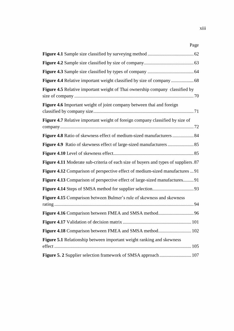
xiii
Page
Figure 4.1 Sample size classified by surveying method ....................................... 62
Figure 4.2 Sample size classified by size of company .......................................... 63
Figure 4.3 Sample size classified by types of company ....................................... 64
Figure 4.4 Relative important weight classified by size of company ................... 68
Figure 4.5 Relative important weight of Thai ownership company classified by
size of company ..................................................................................................... 70
Figure 4.6 Important weight of joint company between thai and foreign
classified by company size..................................................................................... 71
Figure 4.7 Relative important weight of foreign company classified by size of
company ................................................................................................................. 72
Figure 4.8 Ratio of skewness effect of medium-sized manufacturers .................. 84
Figure 4.9 Ratio of skewness effect of large-sized manufacturers ...................... 85
Figure 4.10 Level of skewness effect.................................................................... 85
Figure 4.11 Moderate sub-criteria of each size of buyers and types of suppliers . 87
Figure 4.12 Comparison of perspective effect of medium-sized manufactures ... 91
Figure 4.13 Comparison of perspective effect of large-sized manufactures ......... 91
Figure 4.14 Steps of SMSA method for supplier selection................................... 93
Figure 4.15 Comparison between Bulmer’s rule of skewness and skewness
rating ...................................................................................................................... 94
Figure 4.16 Comparison between FMEA and SMSA method.............................. 96
Figure 4.17 Validation of decision matrix .......................................................... 101
Figure 4.18 Comparison between FMEA and SMSA method............................ 102
Figure 5.1 Relationship between important weight ranking and skewness
effect .................................................................................................................... 105
Figure 5. 2 Supplier selection framework of SMSA approach ........................... 107

1
CHAPTER 1
INTRODUCTION
1.1 Introduction
Nowadays businesses tend to compete with rivals by improving capability to
meet customer demands. In terms of logistics and supply chain management, there are
several activities which a firm should conduct, for example, customer service and
support, purchasing and procurement, transportation, inventory management, etc.
Among these activities, purchasing and procurement is an activity that manufacturing
companies have been facing and focusing due to its significance in company overall
effectiveness (Bevilacqua & Petroni, 2002; Ellram & Carr, 1994). In procurement and
purchasing process, there are six decisions to make orderly (Aissaoui, Haouari, &
Hassini, 2007) as shown in Figure 1.1.
Figure 1.1 Decision processes in purchasing and procurement activity
(Aissaoui et al., 2007)
Make or Buy
Supplier
selection
Contract
negotiation
Design
collaboration
Procurement
Sourcing
analysis
Purchasing
decisions

2
In Figure 1.1, after companies decide whether to make product by themselves
or buy from outside, the next step is supplier selection process which means selecting
the most suitable supplier who should provide materials, parts, semi-finished parts, etc.,
to buyer’s company in order to produce product by their own or sell to customers with
highest efficiency. Then design the contract, how should company negotiate with
selected supplier. Next step is design collaboration, co-working with supplier to meet
product requirement and specification before start the procurement process. After finish
the procurement, company should evaluate efficiency of purchasing and procurement
activity, especially supplier performance. From these decision processes, one of the key
to improve logistics efficiency of a firm is to select appropriate supplier. To compete
with rivals, suppliers play important role on buying firm. Purchasing cost sometimes
contribute more than 50% of total cost of goods sold (Humphreys, Huang, Cadden, &
McIvor, 2007). Therefore it is obviously that supplier performance has effect on firm
performance. On the other hand, supplier selection and evaluation are able to enhance
cost and reduction as well as quality Aksoy and Öztürk (2011)
De Boer, Labro, and Morlacchi (2001) stated that supplier selection processes
were classified into four phases. After define problem, the criteria must be formulated.
Then qualify or pre-select suppliers to reduce number of possible suppliers before
making final decision. One of the important questions is how to identify critical criteria
as well as its importance level. Since Dickson first introduced 23 critical criteria of
supplier selection problem in 1960, many researchers still used Dickson’s criteria to
evaluate suppliers. It appears that cost, delivery and quality are top-3 basic criteria that
most of the studies considered. The next top-2 criteria are production facilities and
capacity, and technical capability. Due to different industry and environment, then
different criteria are selected. Obviously, supplier selection is the decision making
under multiple criteria including qualitative and quantitative criteria that buying firm
should consider.
Moreover as the environmental awareness has been growing, numerous
researchers in supply chain and logistics management has combined this issue into their
researches in many topics. Green manufacturing is one of the crucial issues to enhance
green supply chain management. Therefore, in supplier selection process, a firm should

3
consider criteria of being green supplier chain in terms of promoting green supply chain
management for long-term sustainability. In this research, criteria of green supplier are
brought to consider with other qualitative and quantitative criteria.
In Thailand, electronics industry is one of the most important industries. Also,
refer to Thailand 4.0 development plan, 1 of 10 targeted industries is electronics
industry with total export in 2017 accounted for more than 60 billion as showed in
Figure 1.2.
Source: Office of Industrial Economics, Ministry of Industry Thailand
Figure 1.2 Export value of Thai electronics industry
From Figure 1.2, it can be seen that electronics industry in Thailand is
continuously expanding. With skillful labor, geographic advantage and transport
facilities, Thailand has been being the largest electrical appliances manufacturing base
in ASEAN and will continue to play an important role in Thailand’s economic
development. However, due to ASEAN Economic Community (AEC) that has been
established by the end of 2015, despite of gaining new opportunities, the competition
among this region is more crucial. Thai manufacturers have to adjust themselves for a
situation like this. One of the key issues is improving their performance. Not
2013 2014 2015 2016 2017
electronic appliances 21,596.72 22,439.66 21,415.00 21,906.33 23,703.55
electronics devices 33,107.73 34,417.70 33,885.77 33,179.52 36,505.23
total 54,704.45 56,857.36 55,300.77 55,085.85 60,208.78
0.00
10,000.00
20,000.00
30,000.00
40,000.00
50,000.00
60,000.00
70,000.00
Expo
rt V
alue
(US
D m
ilio
n)

4
surprisingly, supplier selection has positive relationship to buying firm’s performance
(Kannan & Tan, 2002; Nelson, Muhamad, Loo, & Mat, 2005). Improving supplier
selection could affect to manufacturer’s performance as well.
Electronics products are different from general consumer products because they
are various customization and time sensitive which performance extensively depends
on suppliers. In addition, supplier plays a major role in supporting and enhancing
buying firm’s efficiency (Lemke, Goffin, Szwejczewski, Pfeiffer, & Lohmüller, 2000).
There are many researches developing supplier selection method in Asian region. For
example, case study in Hong Kong by Choy, Lee, and Lo (2002), case study in China
by Chiou, Hsu, and Hwang (2008) and Yan (2009), in Taiwan by Lee, Kang, Hsu, and
Hung (2009) and Y. H. Chen and Chao (2012), and the study in Malaysia by
Bhattacharya, Geraghty, and Young (2010). Nevertheless, there appears to be no case
study formulating critical criteria and developing method for supplier selection decision
in Thailand.
Many researchers have been dealing with supplier selection problem for
decades. There are several methods to tackle with this problem. With multiple criteria
of supplier selection, a fashionable method is comparing importance of criteria
assuming that criteria are independent. Then calculate preference score of each
potential supplier without consideration of uncertainties of supplier performance,
especially if the data of performance throughout a periodic of time is not utterly
symmetric, i.e. normal distribution. Therefore, for better reflect to real circumstances,
this research attempts to develop a proper method to select supplier for Thai electronics
manufacturers based on mean-variance-skewness of supplier’s performance regarding
multiple interrelated criteria by using ANP approach.
1.2 Problem Statement
Generally, when selecting supplier, buying firm should select the one which
have high expected performance (i.e., mean) and low risk (i.e., variance). But
consideration only mean and variance may not sufficient as mention earlier because
literally supplier’s performance could be fluctuated for a period of time. That is to say

5
that supplier whose performance has no skewness does not point out that it is good
supplier.
Figure 1.3 Example of on-time delivery performance of possible supplier A-D
For example, in order to evaluate supplier performance based on deliverability
which is measured by %on-time delivery. Supposed that each graph in Figure 1.3
represents on-time delivery performance of different supplier (A-D). To compare
between A and B, both of them has same average %on-time delivery, as mean of these
two suppliers are equal. But the variance of A is greater than B as we can see that graph
A is more spread out than B. In this case we can say that supplier B is better than A
even though their average performances are equal since B’s performance is more stable
or has lower variance. In other words, lower SD means lower risk. But to compare
between C and D, both suppliers has equal mean and SD. If buyer only takes mean and
variance into account, then buyer may conclude that both of them have equal
performance. But if buyer also takes skewness into consideration, despite the fact that
C and D has equal average, both may perform different performance. Figure (C) shows
that its performance skews to the right (positive-skew) while (D) skews to the left
(A) (B)
Standard deviation of A Standard deviation of B
Average
performance
(D) (C)
Average
performance
Standard deviation of C Standard deviation of D

6
(negative-skew). This means that most likely C has lower %on-time delivery than
expected while D has higher since D’s mode exceeds means and vice versa for C.
Assuredly, buyers prefer left-skewed %on-time delivery to either right-skewed or
symmetrical of %on-time delivery distribution. The question is, whether skewness has
effect and plays important role on supplier performance.
Please be noted that there is 2 types of performance. One is performance with
negative skewness is preferred or the higher of performance index, the better efficiency,
such as %on-time delivery. Conversely, another one is performance with positive
skewness is preferred or the lower of performance index, the better efficiency, such as
cost and lead time. In this case buyers would prefer right-skewed rather than left-
skewed performance.
Even there is an evaluating performance combines these 3 combinations
together which is called mean-variance-skewness framework and often used in
portfolio selection problem. In the problem of portfolio selection, the investor must
select the optimal portfolio. To evaluate or measure portfolio performance, there is a
method to evaluate based on mean-variance-skewness framework. The results prove
that the efficiency obtained from combining those three moments is better than
traditional evaluation. But in logistics research, no one ever applied this concept on
supplier selection problem. This research aims to fill these gaps by developing decision
matrices for selecting proper supplier with multiple interrelated criteria based on mean-
variance-skewness of supplier’s performance to enhance higher purchasing efficiency
of buying firm.
1.3 Research Questions
From problem statement as explained in previous section, there are 2 research
questions as follows:
1. Do the skewness has effect on performance?
2. If the answer is yes, should decision maker considers skewness on top of the
average and standard deviation when selecting supplier and what is the proper method?
7
1.4 Research Objectives
1. To identify influential criteria and their important weight of supplier selection
problem for Thai electronics industry.
2. To develop decision matrices for selecting supplier based on mean-variance-
skewness of supplier’s performance.
1.5 Research Methodology
After formulating criteria set which is gathered by literature review, then the
questionnaire is designed in order to collect the data which has 2 types. The first type
of data is the comparison among criteria to identify criteria important weight. This data
will be analyzed using ANP approach. Another type is the data of performance
evaluating in order to obtain the value of supplier performance in 3 characteristics,
which is mean, standard deviation, and skewness. Then this data will be analyzed to
explore skewness effect. Finally both type of data will be combined together in order
to develop decision matrix.
1.6 Contribution
The main contribution of this research has two-folds. One is contribution for
Thailand industry and another one is contribution for academic. For Thailand industry’s
contribution, this research will provide the appropriate systematic to help electronics
industry in Thailand select the most suitable supplier in a practical way. For academic
contribution, this research is the first one applying the concept of performance
evaluation based on mean-variance-skewness framework on supplier selection problem
and explore the importance of criteria of green supplier to enhance supply chain
management sustainability.

8
CHAPTER 2
LITERATURE REVIEW
The main objective in this research is to develop decision matrices for selecting
appropriate supplier with multiple interrelated criteria under risk consideration in order
to enhance logistics efficiency of Thai electronics industry. This chapter will present
related previous study including theory and principle that will be applied in this research.
In order to achieve research objectives, literature review in this research is classified
into 5 main topics.
1. Supplier selection criteria to extract influential criteria and construct initial
set of criteria used in this research.
2. Supplier selection method to study methods that researchers used in supplier
selection problem in order to identify suitable method for this research.
3. AHP and ANP approach which is the approach used in this research.
4. Performance evaluating to show the idea of skewness impact on supplier
selection and the idea of bringing skewness into performance evaluation.
5. FMEA concept which is the measurement of potential failure in order to
acquire the idea of new method for supplier selection.
2.1 Supplier Selection Criteria
In logistics and supply chain management, one of the key activities is
procurement and purchasing activity. It is impossible to process all activities in order
to manufacture products to end-customer in one place or one company. In reality
businesses have been more relied on suppliers (Simić, Kovačević, Svirčević, & Simić,
2017). One of the important question on supplier selection problem is what are the
critical criteria affecting to the decision process and how to measure the importance
level of each criterion. Back to 1966, Dickson introduced 23 critical factors which
affecting vendor selection and evaluation by spreading out questionnaire to purchasing
agents and managers in United States and Canada. Among these 23 criteria, Dickson’s
survey revealed that the top 6 important criteria were quality, delivery, performance

9
history, warranties and claim policies, production facilities and capacity, and price,
respectively. Notwithstanding that this study was published since 1966, some of criteria
are still valid and considered as affecting factor on supplier selection by many
researchers. After Dickson’s study in 1966, Weber, Current, and Benton (1991)
conducted research and reviewed about criteria and methods which had been studied
by researchers since 1966-1990. From his review, it was found that price, quality and
delivery were extremely influent to select a proper supplier. The next ranks are
production facilities and capacity, geographical location, and technical capability,
respectively. The different weight could come from changing of business and
manufacturing environment. Table 2.1 shows comparison of ranking of criteria between
Dickson (1966) and Weber et al. (1991).
Table 2.1 Criteria ranking between Dickson (1966) and Weber et al (1991)
No. Criteria Dickson’s
rank
Weber et al.’s
rank
1 Quality 1 3
2 Delivery 2 2
3 Performance history 3 9
4 Warranties and claim policies 4 23
5 Production facilities and capacity 5 4
6 Price 6 1
7 Technical capability 7 6
8 Financial position 8 9
9 Procedural compliance 9 15
10 Communication system 10 15
11 Reputation and position in industry 11 8
12 Desire for business 12 21
13 Management and organization 13 7
14 Operating controls 14 13
15 Repair service 15 9
16 Attitude 16 12
17 Impression 17 15
18 Packaging ability 18 13
19 Labor relations record 19 15
20 Geographical location 20 5
21 Amount of past business 21 21
22 Training aids 22 15
23 Reciprocal arrangements 23 15

10
Since 1990s, many researches have been using Dickson’s criteria to evaluate
supplier. Apparently, cost, quality and delivery are the basic criteria that most of the
studies considered. For example, Weber and Desai (1996) tried to measure supplier
performance and efficiency based on combination of three basic performances required
criteria, namely cost, quality, and delivery. De Boer, Van Der Wegen, and Telgen
(1998)also considered cost and quality as major criteria that buying firm should
concerned but location of supplier and supplier’s yearly turnover were added in to the
decision model. The reason was in JIT production system; supplier should not be
located too far from manufacturing firm and should not too small or too big for buying
firm to manage. Verma and Pullman (1998) did research about how managers choose
suppliers and trade-off among four influential criteria, which are cost, quality, delivery,
and flexibility. By surveying from questionnaire sent to 139 metallic tooling
manufacturers in Western United States, it was found that quality is the most important
criteria, followed by on-time delivery, cost, lead time and flexibility, respectively.
Similar to Verma and Pullman’s study, Albino and Garavelli (1998) considered cost,
quality, and delivery as basic performances with management skill of supplier and
technical capability when making decision while Ghodsypour and O'Brien (1998) and
Ghodsypour and O’Brien (2001) included production facilities and capacity to be one
of their criteria.
Under the assumption of product quality among alternate suppliers are identical,
Cakravastia, Toha, and Nakamura (2002) selected cost and on time delivery to be
critical factors as they implied in their study that to satisfy end customers is comprised
of price and lead time. Choy et al. (2002) used the case-based reasoning (CBR) and
neural network (Kannan & Tan) approaches to evaluate and select supplier into 2 stages.
First is to retrieve potential supplier lists then benchmarking suppliers in the list to
select the best one among potential suppliers. Five criteria were considered in the final
decision. Four of them were taken from Dickson’ criteria, namely, cost, quality,
delivery, and supplier financial. Also one additional criterion, customer service, was
added other than Dickson’s. Katsikeas, Paparoidamis, and Katsikea (2004) did the
study to examine supplier performance based on buying decision criteria of cost, quality,
delivery, technical capability, procedural compliance. Also this is one of few studies
which brought criteria of warranties and claim policies back to decision model.

11
It is noticed that lately, in researches on supplier selection problem, number of
critical criteria taken into account has been increasing with more complex decision
structure. For example, other than consideration of basic criteria, Gencer and Gürpinar
(2007) also considered other critical factor when developing decision model to select
supplier in an electronics company. Totally, 12 criteria from Dickson’s study had been
taken into account. Bhattacharya et al. (2010) selected 9 criteria from Dickson 23
criteria to be considered same as Xiao, Chen, and Li (2012) but different criteria were
concerned. The criteria of each study are shown in Table 2.2, as well as other researches
that are mentioned above.
Moreover, since the 21st century has been started, the concerning of green
logistics and supply chain management has been growing. Some of researchers have
brought green issue to be one of critical factor when making selecting supplier. For
example, Li and Zhao (2009), Yan (2009), Mafakheri, Breton, and Ghoniem (2011), Y.
H. Chen and Chao (2012), included greenness criteria into their decision model. Chiou
et al. (2008), compared ranking of critical criteria including green concerning among
American, Japanese and Taiwanese Electronics Industry in China. The result showed
that all 3 basic performances, cost, quality, and delivery still had importance more than
greenness of supplier. Similar to the study of Lee et al. (2009), this study implied that
buying firms preferred criteria which related to their efficiency such as cost, quality,
delivery, and technical capability rather criteria of being green supplier. However,
environmental issue has been continuously increasing its importance. Thus, a green
supplier criterion is considered as one of critical criteria in this research.
Apparently supplier selection is multi-criteria decision making. Also not only
quantitative criteria should buying firm consider but also qualitative criteria
Ghodsypour and O'Brien (1998). Selecting a suitable supplier is trading off among
those influential factors. Table 2.2 shows influential criteria on supplier selection
problem used in previous researches. It should be noted that some criteria are renamed
to match with Dickson’s criteria depending on its definition.
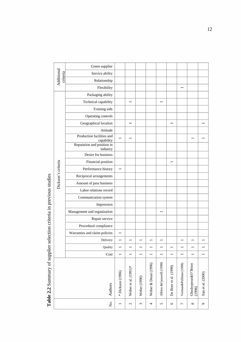
12
Tab
le 2
.2 S
um
mar
y o
f su
ppli
er s
elec
tion c
rite
ria
in p
revio
us
studie
s
A
ddit
ional
crit
eria
Green supplier
Service ability
Relationship
Flexibility 1
Dic
kso
n’s
cri
teri
a
Packaging ability
Technical capability 1 1
Training aids
Operating controls
Geographical location 1 1 1
Attitude
Production facilities and
capability
1
1 1
1
Reputation and position in
industry
Desire for business
Financial position 1
Performance history 1
Reciprocal arrangements
Amount of pass business
Labor relations record
Communication system Impression
Management and organization 1
Repair service
Procedural compliance
Warranties and claim policies 1
Delivery 1
1
1
1
1 1
1
1
Quality 1
1
1
1
1
1
1
1
1
Cost 1
1
1
1
1
1
1
1
1
Auth
ors
* D
ick
son
(1
99
6)
Web
er e
t al
. (1
99
1)*
Web
er (
19
96
)
Web
er &
Des
ai (
19
96
)
Alb
ino &
Gar
avel
li (
1998)
De
Bo
er e
t al
. (1
998
)
Ver
man
&P
ull
man
(1998)
Gho
dsy
po
ur&
O’B
rien
(199
8)
Jian
et
al. (2
000
)
No
.
1
2
3
4
5
6
7
8
9
13
Addit
ional
crit
eria
Green supplier 1
1
1
1
Service ability 1 1
1 1
1
Relationship 1
Flexibility 1
Dic
kso
n’s
cri
teri
a
Packaging ability 1
Technical capability 1
1 1
1
Training aids 1
Operating controls 1
Geographical location 1 1
Attitude 1
Production facilities and
capability
1 1 1
Reputation and position in
industry
1
Desire for business
Financial position 1 1 1
Performance history
Reciprocal arrangements
Amount of pass business
Labor relations record
Communication system 1 1
1
Impression
Management and organization 1 1
1
Repair service
Procedural compliance 1
Warranties and claim policies 1
Delivery 1
1
1
1
1
1
1 1
Quality 1 1
1
1
1
1
1
1
Cost 1
1
1
1 1
1 1
Auth
ors
Gho
dsy
po
ur
& O
’Bri
en
(200
1)
Cak
rav
asti
a et
al.
(200
2)
Ch
oy
et
al. (2
002
)
Kat
sik
eas
et a
l. (
200
4)
Gen
cer&
Gu
rpin
a
(200
7)
Ch
iou
et
al. (2
00
8)
Lee
et
al. (2
009
)
Li
& Z
hao
(20
09
)
Yan
(20
09
)
No
.
10
11
12
13
14
15
16
17
18

14
Addit
ional
crit
eria
Green supplier 1
Service ability 1
Relationship 1
1
Flexibility 1 1 1
Dic
kso
n’s
cri
teri
a
Packaging ability
Technical capability 1 1
1
1
1
Training aids 1
Operating controls
Geographical location 1 1
Attitude 1
Production facilities and
capability
1
1
1
1
Reputation and position in
industry
1 1
Desire for business
Financial position 1 1
1
Performance history 1
Reciprocal arrangements Amount of pass business
Labor relations record
Communication system 1
Impression
Management and organization 1 1
Repair service
Procedural compliance 1 1
Warranties and claim policies 1
Delivery 1
1
1
1
1
1
1
Quality 1
1
1
1
1
1
1
Cost 1
1
1 1
1
Auth
ors
Bh
atta
char
ya
et a
l.
(201
0)
Ak
soy
& O
ztu
rk (
20
11
)
Maf
akh
eri
et a
l. (
20
11
)
Y.H
. C
hen
& C
hao
(201
2)
Xia
o e
t al
. (2
012
)
P-S
. C
hen
& W
u (
20
13
)
Dar
gi
et a
l. (
20
14
)
No
.
19
20
21
22
23
24
25
15
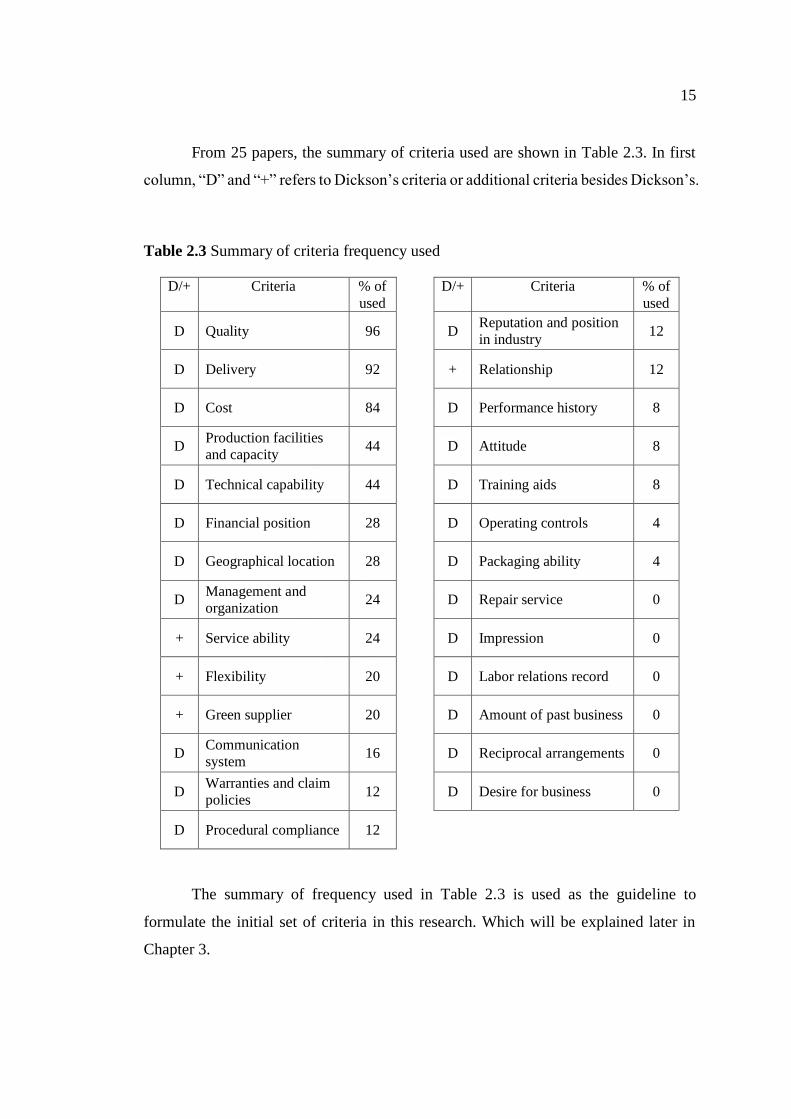
From 25 papers, the summary of criteria used are shown in Table 2.3. In first
column, “D” and “+” refers to Dickson’s criteria or additional criteria besides Dickson’s.
Table 2.3 Summary of criteria frequency used
D/+ Criteria % of
used
D/+ Criteria % of
used
D Quality 96 D Reputation and position
in industry 12
D Delivery 92 + Relationship 12
D Cost 84 D Performance history 8
D Production facilities
and capacity 44 D Attitude 8
D Technical capability 44 D Training aids 8
D Financial position 28 D Operating controls 4
D Geographical location 28 D Packaging ability 4
D Management and
organization 24 D Repair service 0
+ Service ability 24 D Impression 0
+ Flexibility 20 D Labor relations record 0
+ Green supplier 20 D Amount of past business 0
D Communication
system 16 D Reciprocal arrangements 0
D Warranties and claim
policies 12 D Desire for business 0
D Procedural compliance 12
The summary of frequency used in Table 2.3 is used as the guideline to
formulate the initial set of criteria in this research. Which will be explained later in
Chapter 3.

16
2.2 Supplier Selection Method
Based on research methodology, after formulating criteria has been done, the
next issue to be determined is what is the proper supplier selection method should be
used in this research. From study of De Boer et al. (2001) supplier selection processes
were classified into 4 phases as shown in Figure 2.1. First is to define the problem, what
exactly the aim of problem is and what a firm wants to achieve. Then formulate set of
critical criteria before qualifying process of suitable suppliers to obtain a set of potential
suppliers. In other words, pre-select suppliers to reduce number of possible suppliers.
Then make the final decision and select the most appropriate supplier.
Figure 2.1 Decision methods in supplier selection processes
(modified from De Boer et al. (2001))
From these processes, it indicates that in there are two steps of selection, one is
pre-selection and another one is final selection. Therefore, this topic is separated into 2
sections. First section is method to pre-qualify supplier. The second one is method to
make final selection.
Qualification
Problem
formulation
Formulation of
criteria
Final selection
Buy/not buy?
More/fewer suppliers?
Replacing current
suppliers?
Previously used criteria
available?
More/fewer criteria?
Selection steps

17
2.2.1 Method of Supplier’s Pre-qualification Phase
As mention in previous paragraph, pre-qualification phase or pre-selection
phase is the process to reduce number of potential suppliers before making final
decision. So the idea of this phase is mainly classification suppliers into groups. Then
the decision maker can select group of suppliers that has highest potential than other
groups. From literature review, it is found that there are 4 decision methods dealing
with pre-selection step, i.e. categorical methods, data envelopment analysis (DEA),
cluster analysis (CA), and case based reasoning (CBR).
- Categorical Method
Categorical method is a method to evaluate supplier’s performance by
categorical judging from decision maker. The buying firm evaluates each alternate
supplier’s performance on each criteria as either, good (positive), moderate (neutral) or
inefficient (negative), then summarize the overall rating (Timmerman, 1986). The
shortcoming of this method is all criteria are assumed to have same important weight
that is reflect to real decision making.
- Cluster Analysis (CA)
The next method is cluster analysis (CA). CA is the statistical classification
technique to divide data into groups or clusters. A research by Holt (1998) applied this
approach to supplier selection problem. In supplier selection problem, data is the whole
list of suppliers. By classifying suppliers based on their performance, all suppliers are
allowed to be separated into groups or clusters. The variance of performance within
clusters is small or homogeneous but variance between clusters is large or
heterogeneous. Generally we can say that suppliers in the same cluster have similar
performance whereas suppliers in different clusters have different performance. Then,
buying firm is able to select cluster or group of supplier which has higher performance
compared with other groups to be potential suppliers. Therefore, the numbers of
potential suppliers are reduced. This method is well pre-qualifying suppliers.
18
- Data Envelopment Analysis (DEA)
One of the well-known methods to pre-select suppliers is data envelopment
analysis (DEA). DEA is the technique used to compare performance efficiency of
decision making units (DMUs) developed by Charnes et al. (1978). In DEA technique,
all DMUs are evaluated its output efficiency based on its input and classified into two
groups which judging by efficiency score of each. The maximum efficiency score is
equal to one, and the DMUs with maximum efficiency score is call efficient DMUs.
Another one is considered as inefficient DMUs which have efficiency score less than
one.
For supplier selection problem, each DMU refers to each supplier. Applying
this technique, buying firms are able to distinguish between potential suppliers and
incompetent suppliers that are efficient suppliers and inefficient suppliers, respectively.
There are several researches applying DEA to supplier selection problem. For example,
Weber and Desai (1996), based on three criteria of price (i.e. cost), quality, and delivery,
the authors applied DEA to measure supplier’s performance and efficiency. In this
study, there are totally six suppliers to evaluate. One of the benefit of DEA is this
technique is not only be able to evaluate the performance of each supplier but also helps
inefficient vendors to perceive their own relative performances benchmark with
efficient suppliers (Weber, 1996). Other studies of DEA in supplier selection can be
seen in Jian, Fong‐Yuen, and Vinod (2000), Toloo and Nalchigar (2011) and Dobos
and Vörösmarty (2014).
- Case Base Reasoning (CBR)
The last method used for supplier pre-selection phase is case based reasoning
(CBR). Choy et al. (2002) applied this method on supplier pre-qualification stage to
regain list of candidate suppliers before benchmarking candidate suppliers and finalize
who should be selected by using neural network engine (NNE). This method is used
artificial intelligence (AI) technique to solve the problem by using previous similar
situations, information, and knowledge in a huge database. But the shortcoming of this
method is it requires enormous database.

19
2.2.2 Method of Supplier’s Final Decision Phase
The final decision phase is the stage to select the most suitable supplier. This
stage can be done either after finishing pre-quality stage or after getting the whole list
of suppliers, i.e. supplier pre-qualification is omitted. There are several methods to
make final choice in supplier selection problem as follows:
- Mathematical Optimization
In this approach, the decision makers formulate mathematical model based on
the set of constraints to optimize objective function which could be maximization (e.g.
maximizing profit) or minimization (e.g. minimizing cost or lead time of purchasing).
This method could be more objective and quantitative than rating method De Boer et
al. (2001). Weber and Current (1993) proposed multi objective optimization model for
vendor selection. Three objectives were included in their model, which are to minimize
purchasing price (i.e. cost criteria), to minimize late deliver by vendor (i.e. delivery
criteria), and to minimize rejected units (i.e. quality criteria). In the study of
Ghodsypour and O’Brien (2001), not only considering net price of purchasing but this
paper also proposed to select supplier with the objective of minimizing total cost of
logistics, that are, net price, ordering cost, transportation cost and holding cost. Liao
and Rittscher (2007) stated that flexibility provided by suppliers to arrange their
processes and conditions is important. Therefore with multi objectives comprised of
cost minimization, quality rejection rate minimization, late delivery minimization and
flexibility maximization, together with constraints of customer demand, supplier’s
capacity the authors formulated model to select supplier.
There are some researcher combines mathematical optimization methods with
other approaches, for example, Mafakheri et al. (2011). In this paper, two types of cost,
purchasing cost and inventory holding cost which related to quantities ordered, were
considered as objective functions. Considering time varying of purchasing cost and
inventory holding cost, dynamic function of those bi-objectives were formulated.
However, the characteristics of supplier selection problem are hard to formulate
mathematical model Weber and Current (1993). So the great disadvantage of this
20
technique is with the greater number of variables of factors, the more complex and
harder to solve the problem.
- Artificial Intelligence (AI) and Neural Network (Kannan & Tan)
Artificial Intelligence (AI) is computer science to simulate human intelligence
by training computers to understand human’s intellect to compute or to solve the
problem in terms of achieving the goal. It is like imitating human reaction based on
historical data or previous experience. One of method based on AI that researchers used
to solve supplier selection problem is neural network (Kannan & Tan). In NN method,
it is not necessary to formalize the process of decision making and this is well reflect
to real situation as NN can cope with uncertainty and complication De Boer et al. (2001).
Albino and Garavelli (1998) propose NN to evaluate subcontractors in construction
firms. With set of input parameter, i.e. selection criteria, the network is trained by the
examples of training set. Once the training process is done, the network is tested
accuracy. Finally by giving a real data set of competitors, i.e. potential suppliers, the
network can evaluate potential suppliers and provide final competitor rating to decision
maker.
Choy et al. (2002) applied CBR technique and NN to select and benchmark
suppliers for case study of consumer product companies in Hong Kong. Case base
reasoning technique is used in pre-selection stage as mentioned in previous section, and
then NN is used to finalize the decision. Another study that presented NN approach to
supplier selection problem is done by Aksoy and Öztürk (2011). To overcome the
drawback of traditional selection and evaluation approaches, that are the complexity of
decision process with multiple attributes and the uncertainties, the authors introduced
NN approach to support supplier selection process focusing on just-in-time (JIT)
manufacturers based on four criteria, which are quality, delivery, location of supplier,
and price. As stated earlier, the advantage of NN is this approach does not need decision
making process formulation and well handle uncertain and complicated situation.
However, NN requires enormous database. Also the process between input and output
layer is like a black box and hard to trained the network.
21
- Multi Criteria Decision Making (MCDM) Technique
It is no doubt that supplier selection is multi-criteria decision making problem.
Many MCDM techniques have been used to tackle with this decision problem. For
example, analytic hierarchy process (AHP), analytic network process (Eshtehardian,
Ghodousi, & Bejanpour), and fuzzy theory.
In AHP and ANP approaches, all criteria are weighed and alternatives are
ranked based on pairwise comparison. These approaches are able to deal with both of
quantitative and qualitative criteria and simplify complex problem into hierarchical
form. For example, Ghodsypour and O'Brien (1998) applied AHP technique to
determine important weight of criteria as well as overall score of alternate suppliers. Li
and Zhao (2009) used AHP to select the most suitable for automotive industry. Similar
to Chen and Wu’s study in 2013, but this research applied AHP technique to select
supplier for semiconductor manufacturer. Although AHP is a well-known method but
it has some shortcoming as in AHP, the relationship among criteria are ignored and
assumed to be independent. Consequently, some researchers try to overcome this
shortcoming by applying ANP approach, for example, the study of Gencer and
Gürpinar (2007) and Xiao et al. (2012).
In traditional AHP and ANP, the decision makers make pairwise comparison by
giving the exact number of preference but in reality, human preference is hard to attain.
For this reason, fuzzy theory has brought into MCDM technique. Chiou et al. (2008)
proposed fuzzy analytic hierarchy process (FAHP) for case study of overseas
electronics industry in China. After collecting pairwise comparisons from decision
maker, the result are transformed in to fuzzy number using triangular fuzzy number.
Lee et al. (2009) also applied fuzzy set theory using fuzzy extended AHP (FEAHP)
which is the method carried out by triangular fuzzy numbers then uses extend analysis
method to determine value of pairwise comparison. This research is applied on the case
study of LCD industry in Taiwan. Fuzzy theory is not only applied on AHP but also
ANP as well. Dargi, Anjomshoae, Galankashi, Memari, and Tap (2014) used fuzzy
ANP (FANP) to determine the important weight of criteria and applied this method on
the case study of Iranian automotive company.

22
- Hybrid method
To develop the better accurate method dealing with supplier selection problem,
some researches combine more than one approach together. Ghodsypour and O'Brien
(1998) combined AHP and linear programming (LP) on two-stage supplier selection
problem. First AHP was used to determine rating of each alternate supplier. Then, LP
optimization was used to find the best supplier and its order quantity aimed to maximize
total value of purchasing. Yan (2009) implemented hybrid method combining AHP and
genetic algorithm (GA) to better calculate weight score and rank the alternate suppliers.
Bhattacharya et al. (2010) conducted a research by combining AHP and quality function
deployment (QFD). QFD is the tool to let a firm knows customer’s needs and
expectation, i.e. voice of customer. Firstly, all criteria are classified into 2 groups. One
is criteria related to customer requirement, such as delivery, quality, etc. Another group
is criteria related to engineering requirement, such as company’s infrastructure and
facility. After developing QFD matrix, important weights of criteria obtain from QFD
matrix are used as the pairwise comparison to calculate utility value (priority vector in
AHP). Then a decision maker can rank the alternate suppliers and select the most
suitable one.
Furthermore, there are other hybrid methods, for example, the combination of
DEA, decision tree and NN presented by Wu (2009)
- Other methods
In addition above approaches, there are other methods proposed by researchers.
For example, Verma and Pullman (1998) explored important level of supplier selection
criteria, cost, quality, delivery, and flexibility by surveying using linker scale
questionnaire. Then used discrete choice regression analysis to acquire weight (i.e.
regression coefficient).
23
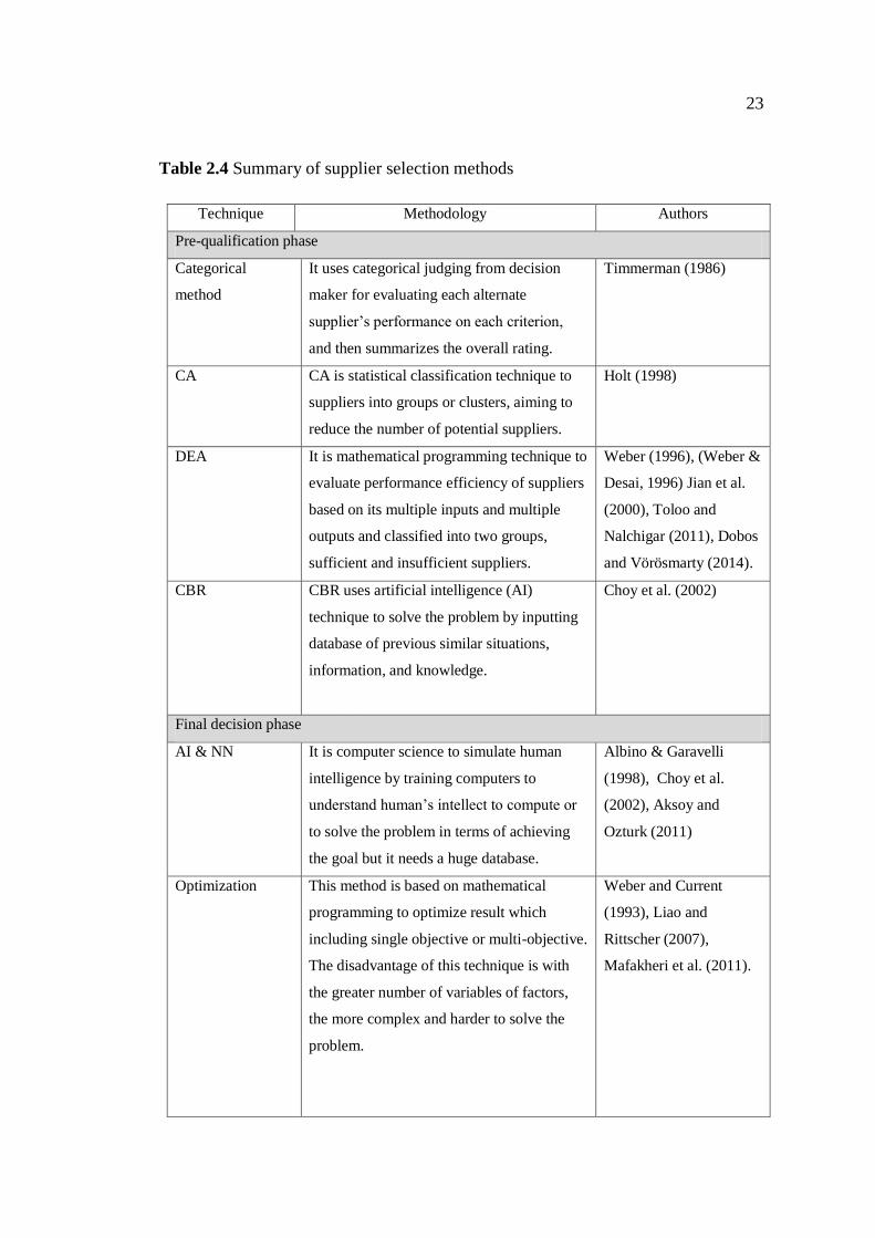
Table 2.4 Summary of supplier selection methods
Technique Methodology Authors
Pre-qualification phase
Categorical
method
It uses categorical judging from decision
maker for evaluating each alternate
supplier’s performance on each criterion,
and then summarizes the overall rating.
Timmerman (1986)
CA CA is statistical classification technique to
suppliers into groups or clusters, aiming to
reduce the number of potential suppliers.
Holt (1998)
DEA It is mathematical programming technique to
evaluate performance efficiency of suppliers
based on its multiple inputs and multiple
outputs and classified into two groups,
sufficient and insufficient suppliers.
Weber (1996), (Weber &
Desai, 1996) Jian et al.
(2000), Toloo and
Nalchigar (2011), Dobos
and Vörösmarty (2014).
CBR CBR uses artificial intelligence (AI)
technique to solve the problem by inputting
database of previous similar situations,
information, and knowledge.
Choy et al. (2002)
Final decision phase
AI & NN It is computer science to simulate human
intelligence by training computers to
understand human’s intellect to compute or
to solve the problem in terms of achieving
the goal but it needs a huge database.
Albino & Garavelli
(1998), Choy et al.
(2002), Aksoy and
Ozturk (2011)
Optimization This method is based on mathematical
programming to optimize result which
including single objective or multi-objective.
The disadvantage of this technique is with
the greater number of variables of factors,
the more complex and harder to solve the
problem.
Weber and Current
(1993), Liao and
Rittscher (2007),
Mafakheri et al. (2011).

24
Technique Methodology Authors
Final decision phase
MCDM
techniques
MCDM techniques are the techniques to
help decision maker to make decision based
on multiple criteria with different weight
importance.
Ghodsypour & O’brien
(1996), Gencer &
Gurpina (2007), Chiou et
al. (2008), Lee et al.
(2009), Li & Zhao
(2009), Xiao et al.
(2012), Chen & Wu
(2013), Dargi et al.
(2014)
Hybrid method It is the combination of more-than-one
approach to solve problem of supplier
selection to gain better efficiency.
Ghodsypour & O’brien
(1998). Yan (2009),
Bhattacharya et al.
(2010), Wu (2009).
Others For example, regression analysis Verma & Pullman
(1998)
2.2.3 Selection Method Comparison
As mention earlier that there are 2 decision phases in supplier selection, which
are, pre-qualification phase and final decision phase. From literature review, it is found
that some methods are well used in decision phase of pre-qualification which is the decision to distinguish between potential suppliers and non-potential suppliers. But
among potential suppliers, it is necessary to use other method in order to decide of who
is the most suitable suppliers. The pros and the cons of each method are summarized
and shown in Table 2.5 and Figure 2.2.

25
Tab
le 2
.5 C
om
par
ison a
mong s
elec
ting m
ethod
Cons
• V
ery s
ubje
ctiv
e an
d h
ard t
o j
udge
• E
ver
y c
rite
ria
are
assu
med
to h
ave
sam
e le
vel
of
pre
fere
nce
.
• C
an o
nly
sep
arat
e pote
nti
al s
uppli
ers
from
all
alte
rnat
ive
suppli
ers
but
not
giv
e th
e an
swer
of
the
bes
t su
ppli
er.
• N
orm
ally
use
d f
or
quan
tita
tive
crit
eria
.
• C
an o
nly
sep
arat
e p
ote
nti
al s
uppli
ers
from
all
alte
rnat
ive
suppli
ers
but
not
giv
e th
e an
swer
of
the
bes
t su
ppli
er.
•
Nee
d e
norm
ous
dat
abas
e.
• V
ery c
om
ple
x b
ut
can o
nly
sep
arat
e bet
wee
n
pote
nti
al a
nd n
on
-pote
nti
al s
uppli
ers.
• It
is
subje
ctiv
e m
ethod w
hic
h d
epen
ds
on t
he
judgm
ent
of
dec
isio
n m
aker
s.
• N
orm
ally
use
d f
or
quan
tita
tive
crit
eria
.
• H
ard t
o f
orm
ula
te t
he
model
and n
ot
flex
ible
in
the
real
lif
e.
• V
ery c
om
pli
cate
d a
nd n
eeds
a huge
dat
abas
e.
Pro
s
• V
ery e
asy a
nd s
imple
conce
pt
• B
e ab
le t
o d
eal
wit
h b
oth
of
qual
itat
ive
and
quan
tita
tive
crit
eria
• A
ble
to d
eal
wit
h l
arge
num
ber
of
suppli
ers.
• C
an r
educe
s th
e pro
bab
ilit
y t
o r
ejec
t 'g
ood’
suppli
er t
oo e
arly
in t
he
pro
cess
via
subje
ctiv
e
• It
is
wil
dly
use
d s
tati
call
y m
ethod s
o i
ts c
once
pt
is n
ot
new
and t
oo c
om
ple
x, an
d a
lso i
t is
fam
ilia
r to
most
sta
tist
ical
soft
war
e
• P
rovid
e th
e guid
ance
of
how
inef
fici
ent
suppli
ers
nee
d t
o i
mpro
ve
them
selv
es t
o b
ecom
e ef
fici
ent
suppli
ers.
• V
ery f
lexib
le a
nd b
ette
r-re
flec
t re
al w
orl
d
situ
atio
n a
s it
use
s A
I te
chniq
ue.
• B
e ab
le t
o d
eal
wit
h b
oth
of
qual
itat
ive
and
quan
tita
tive
crit
eria
.
•
Be
able
to d
eal
wit
h b
oth
of
qual
itat
ive
and
quan
tita
tive
crit
eria
.
• T
he
answ
er i
s opti
miz
atio
n.
• L
ess
confl
ict.
•
Wel
l han
dle
unce
rtai
n a
nd c
om
pli
cate
d s
ituat
ion.
Phas
e
Fin
aliz
e
Pre
-qual
ify
Pre
-qual
ify
Pre
-qual
ify
Fin
aliz
e
Fin
aliz
e
Fin
aliz
e
Met
hod
Cat
egori
cal
met
hod
Clu
ster
Anal
ysi
s
DE
A
CB
R
AH
P
AN
P F
uzz
y
Mat
h M
odel
NN
26
P
has
e
Fin
al d
ecis
ion
Categorical method
Math model
AHP
ANP
NN
Fuzzy
Pre
-qu
alif
icat
ion
DEA
CBR
Cluster analysis
Qualitative Quantitative Qualitative and
Quantitative
Type of criteria
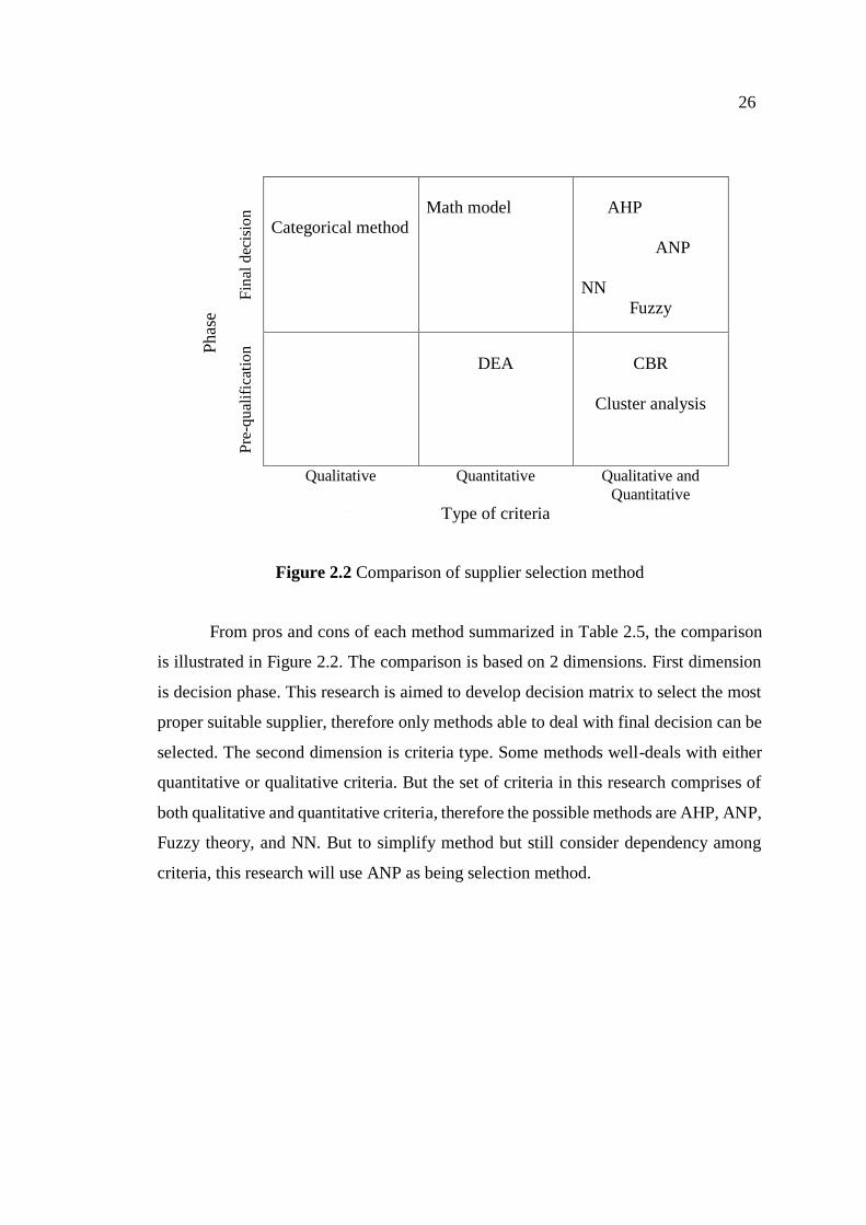
Figure 2.2 Comparison of supplier selection method
From pros and cons of each method summarized in Table 2.5, the comparison
is illustrated in Figure 2.2. The comparison is based on 2 dimensions. First dimension
is decision phase. This research is aimed to develop decision matrix to select the most
proper suitable supplier, therefore only methods able to deal with final decision can be
selected. The second dimension is criteria type. Some methods well-deals with either
quantitative or qualitative criteria. But the set of criteria in this research comprises of
both qualitative and quantitative criteria, therefore the possible methods are AHP, ANP,
Fuzzy theory, and NN. But to simplify method but still consider dependency among
criteria, this research will use ANP as being selection method.
27
2.3 Analytic Hierarchy Process (AHP) and Analytic Network Process
As explained in the previous section, ANP is selected as a tool to determine
weight of criteria on supplier selection problem. Therefore, this section explains about
the principle and fundamental concept of this approach. ANP approach is built on the
concept of AHP method to fill the limitation of traditional AHP that criteria are assumed
to be independent. To explain about ANP, it is necessary to explain about AHP first.
Therefore, literature review in this topic is separated into two parts. First is about AHP,
and the next part is about ANP.
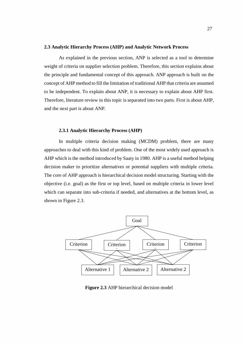
2.3.1 Analytic Hierarchy Process (AHP)
In multiple criteria decision making (MCDM) problem, there are many
approaches to deal with this kind of problem. One of the most widely used approach is
AHP which is the method introduced by Saaty in 1980. AHP is a useful method helping
decision maker to prioritize alternatives or potential suppliers with multiple criteria.
The core of AHP approach is hierarchical decision model structuring. Starting with the
objective (i.e. goal) as the first or top level, based on multiple criteria in lower level
which can separate into sub-criteria if needed, and alternatives at the bottom level, as
shown in Figure 2.3.
Figure 2.3 AHP hierarchical decision model
Goal
Criterion 1
Criterion
2
Criterion
3
Criterion
4
Alternative 1 Alternative 2 Alternative 2

28
The basic concept of AHP is to obtain important weight of each criteria, then
calculate score of each alternative based on all criteria and rank the alternatives. The
comparison of importance among criteria and preference among alternatives uses
pairwise comparison. The steps of AHP can summarized into 5 steps as follows:
1. Construct the decision hierarchy model (i.e. decision tree). After identifying
goal of problem at the top level, affecting factor or criteria must be
determined. Then construct the hierarchical decision structure.
2. Make pairwise comparisons of criteria and alternatives in the same level.
3. Check the consistency of pairwise judgment and re-do step 2 if needed (i.e.
consistency ratio: CR is greater than acceptable interval).
4. Convert result from pairwise comparisons into important weights.
5. Calculate total score of each alternative and rank the alternatives.
To make pairwise comparisons, the decision maker is required to give
preference number to compare between two items. Normally, the scale of preference
(i.e. intensity of importance) is rated from 1 to 9. The definitions of all numbers are
shown in Table 2.6.
Table 2.6 The fundamental scale for pairwise comparisons (Saaty, 1980, 2008)
Intensity of
Importance Definition Explanation
1 Equal importance Two factors contribute equally to the goal
2 Weak or slight
3 Moderate importance The decision maker slightly prefer one
factor to another
4 Moderate plus
5 Strong importance The decision maker strongly prefer one
factor to another
6 Strong plus
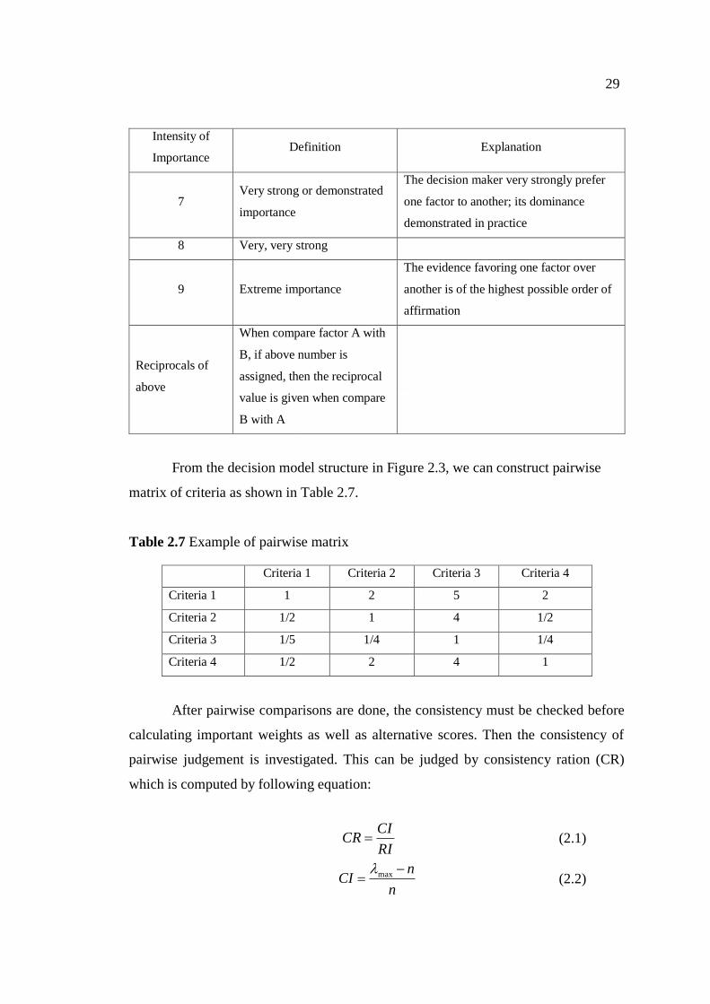
29
Intensity of
Importance Definition Explanation
7 Very strong or demonstrated
importance
The decision maker very strongly prefer
one factor to another; its dominance
demonstrated in practice
8 Very, very strong
9 Extreme importance
The evidence favoring one factor over
another is of the highest possible order of
affirmation
Reciprocals of
above
When compare factor A with
B, if above number is
assigned, then the reciprocal
value is given when compare
B with A
From the decision model structure in Figure 2.3, we can construct pairwise
matrix of criteria as shown in Table 2.7.
Table 2.7 Example of pairwise matrix
Criteria 1 Criteria 2 Criteria 3 Criteria 4
Criteria 1 1 2 5 2
Criteria 2 1/2 1 4 1/2
Criteria 3 1/5 1/4 1 1/4
Criteria 4 1/2 2 4 1
After pairwise comparisons are done, the consistency must be checked before
calculating important weights as well as alternative scores. Then the consistency of
pairwise judgement is investigated. This can be judged by consistency ration (CR)
which is computed by following equation:
RI
CICR (2.1)
n
nCI
max
(2.2)
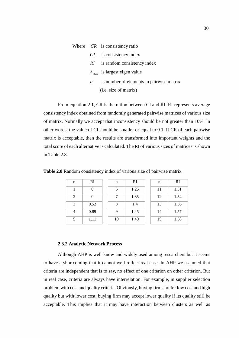
30
Where CR is consistency ratio
CI is consistency index
RI is random consistency index
max is largest eigen value
n is number of elements in pairwise matrix
(i.e. size of matrix)
From equation 2.1, CR is the ration between CI and RI. RI represents average
consistency index obtained from randomly generated pairwise matrices of various size
of matrix. Normally we accept that inconsistency should be not greater than 10%. In
other words, the value of CI should be smaller or equal to 0.1. If CR of each pairwise
matrix is acceptable, then the results are transformed into important weights and the
total score of each alternative is calculated. The RI of various sizes of matrices is shown
in Table 2.8.
Table 2.8 Random consistency index of various size of pairwise matrix
n RI n RI n RI
1 0 6 1.25 11 1.51
2 0 7 1.35 12 1.54
3 0.52 8 1.4 13 1.56
4 0.89 9 1.45 14 1.57
5 1.11 10 1.49 15 1.58
2.3.2 Analytic Network Process
Although AHP is well-know and widely used among researchers but it seems
to have a shortcoming that it cannot well reflect real case. In AHP we assumed that
criteria are independent that is to say, no effect of one criterion on other criterion. But
in real case, criteria are always have interrelation. For example, in supplier selection
problem with cost and quality criteria. Obviously, buying firms prefer low cost and high
quality but with lower cost, buying firm may accept lower quality if its quality still be
acceptable. This implies that it may have interaction between clusters as well as

31
interaction between elements from different level. Thus, it is impossible to construct
decision model in hierarchical structure. To overcome this shortcoming, decision model
is construct and represented by network instead of hierarchical structure. This decision
model is call analytical network or we could say that it is AHP with the assumption of
criteria dependence between cluster and elements was developed, namely, analytic
network process (Eshtehardian et al.) (Saaty, 1999).
From the network in Figure 2.4, criteria C2 has dependence on C1, C3 and C4.
C4 has dependence on C1 and C3, or it is easy to say that there are relationship between
C1 and C4, and between C3 and C4. Also, on the other hand, C3 has dependence on C4.
The loop arrow of each cluster represent the dependence among elements in that cluster.
To make pairwise comparisons among these criteria, the network supermatrix as shown
in Figure 2.5 is constructed.
In Figure 2.5, Ci represents cluster i and eij represents element j in cluster i. For
example, e12 represent element 2 in cluster 1. And wijk represents weight component of
element j in cluster i on jth column. Finally, the result is transformed into important
weight of criteria.
Figure 2.4 Transformation of hierarchical decision structure to network structure
Goal
C1 C2 C3 C4
Goal
Criteria
o o o
Sub-criteria
o o o
Alternative
o o
o o o
o o
o o o o
C1
C2 C3
C4
Hierarchical decision
structure
Network
Structure
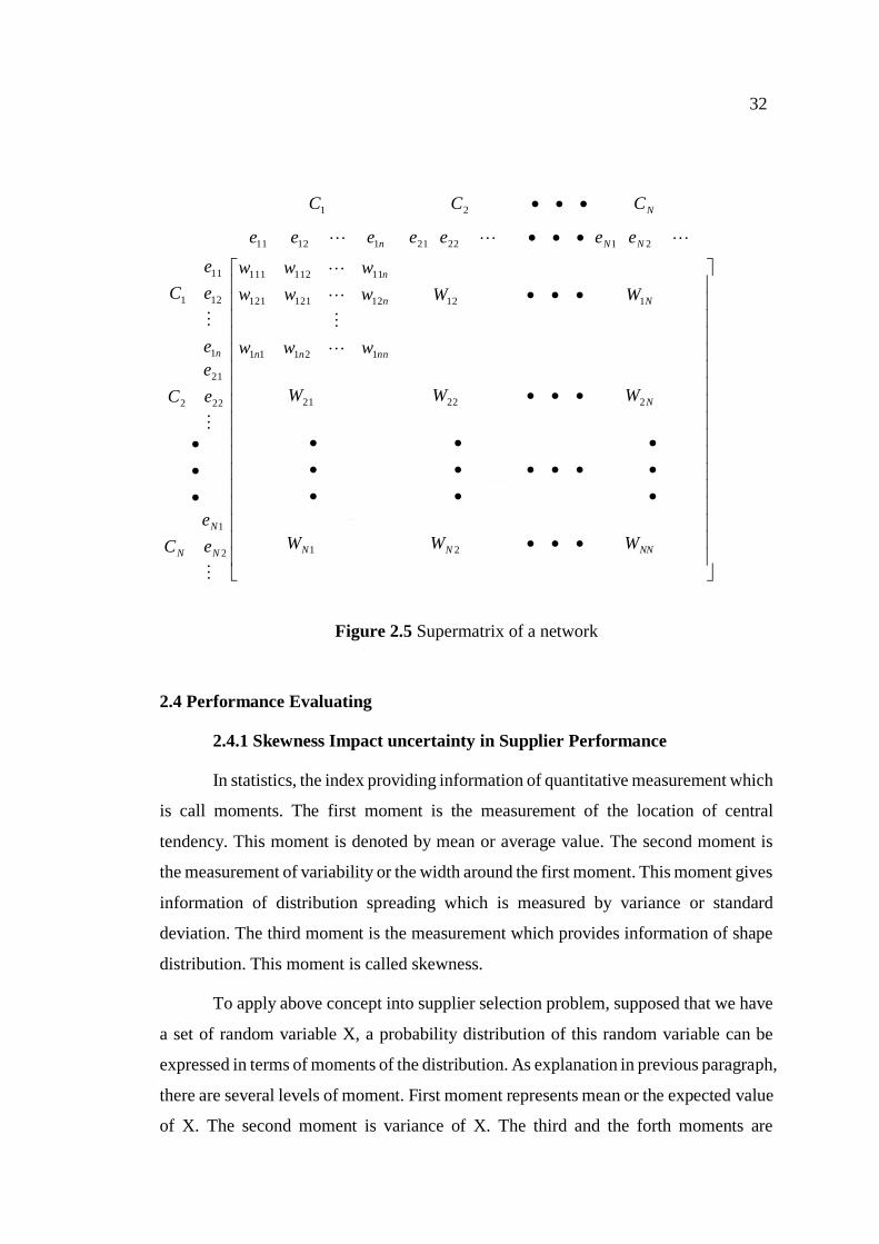
32
NNNN
N
N
nnnn
n
n
NN
N
n
NNn
N
WWW
WWW
WW
www
www
www
eC
e
eC
e
e
eC
e
eeeeeee
CCC
21
22221
112
12111
12121121
11112111
2
1
222
21
1
121
11
21222111211
21
Figure 2.5 Supermatrix of a network
2.4 Performance Evaluating
2.4.1 Skewness Impact uncertainty in Supplier Performance
In statistics, the index providing information of quantitative measurement which
is call moments. The first moment is the measurement of the location of central
tendency. This moment is denoted by mean or average value. The second moment is
the measurement of variability or the width around the first moment. This moment gives
information of distribution spreading which is measured by variance or standard
deviation. The third moment is the measurement which provides information of shape
distribution. This moment is called skewness.
To apply above concept into supplier selection problem, supposed that we have
a set of random variable X, a probability distribution of this random variable can be
expressed in terms of moments of the distribution. As explanation in previous paragraph,
there are several levels of moment. First moment represents mean or the expected value
of X. The second moment is variance of X. The third and the forth moments are

33
skewness (i.e., measuring symmetry of probability distribution) and kurtosis (i.e.,
measuring flatness), respectively (Gujarati, 2003).
Supposed that random variable X representing supplier’s performance. Then the
expected value of supplier’s performance, X, is expressed as E(X). Then the mean,
variance and skewness of supplier’s performance are defined as follows:
Mean; )(XE (1)
Variance; 22)( XEX
(2)
Skewness; 3)( XES X (3)
Where )(XE is expected value of supplier’s performance
is average of supplier’s performance
2
X is variance of supplier’s performance
XS is skewness of supplier’s performance
For example, A company needs to buy raw materials from supplier and 2
options are available, which is buying from supplier A and buying from supplier B.
Supposed that buyer merely concerns on lead time. The historical lead time of both
suppliers are shown in following graphs.

34
Both of supplier A and B have equal average lead time of 15 days. Also there
performance dispersions are approximately equal as their range are 6 days for both of
them. If the decision maker select by judging from average performance and stability,
it may be said that both of them have equal performance. But most likely, supplier A
provides longer lead time than average as its mode is greater than average at about 17
days. In contrary, most likely supplier B can provide shorter lead time than average, as
its mode is equal 14 days. Therefore, actually supplier B is performance better than
supplier A, although their average lead time and standard deviation are equal. In this
case, it suggests that their performance are not symmetrical shape. Performance of
supplier A is skewed to right (greater than average) while performance of supplier B is
skewed to the left (lower than average). The issue to be considered is if buyers should
consider skewness when evaluate suppliers’ performance.
10
12
14
16
18
20
1 2 3 4 5 6 7 8 9 10
LT
(d
ay
s)
10
12
14
16
18
20
1 2 3 4 5 6 7 8 9 10
LT
(d
ay
s)
Supplier A
Average LT =15 days
Max LT = 18 days
Min LT = 12 days
Mode = 17 days
Supplier B
Average LT =15 days
Max LT = 18 days
Min LT = 12 days
Mode = 14 days

35
2.4.2 Mean-Variance-Skewness Performance Evaluations
In financial and economic research, there is a problem of portfolio selection
which the investor should make decision to select the optimal portfolio considering
uncertainties in term of risk aversion. In process of selection, not only expected return
should be considered because the portfolio with greatest expected return does not mean
the most suitable one. That is to say the portfolio with the best expected return is not
necessarily having minimum variance (Markowitz, 1952). Therefore, variance has been
used widely for risk measure (Huang, 2012). To evaluate or measure portfolio
performance, there are many researches on portfolio performance evaluation based on
mean-variance-skewness framework. At the beginning, the researchers evaluate
portfolio based on mean and variance and ignored skewness. The mean-variance model
is introduced by Markowitz in 1952. Supposed that there are n possible choice of
portfolio denoted by X1, X2,...,Xn. Let Ei is the expected return that the investors could
get from each portfolio and Vi is the variance of each alternative. Figure 2.5 shows all
set of (E, V) from all possible choices of portfolio. Each point represents expected
return (mean) and risk (variance) of each portfolio. The border of the surface is called
efficient surface or efficient frontier. The investors should select portfolios which fall
on the border as they are denoted as efficient combinations. Additionally, based on
mean-variance theory, the investors should select portfolios which give maximum
expected return (E) for given variance (V) or less or those with minimum variance for
given expected return (E) or more.
From explanation in previous paragraph, it is clearly that decision making in
portfolio selection is trade-off between return (mean) and risk (variance) for all
portfolio which fall on efficient frontier. Mean-variance model is extensively applied
by many researchers, for example, Fletcher (1994), Chiu and Wong (2011), Castellano
and Cerqueti (2014).

36
Figure 2.6 Combination of mean-variance of possible choice
(modified from Markowitz (1952))
Even though there are a vast study used mean-variance theory, but afterward,
researchers found that the third moment should not be ignored then skewness was
included to evaluate performance. Joro and Na (2006) developed portfolio performance
measurement based on mean-variance-skewness framework and compare the efficiency
obtained from both of mean-variance model and mean-variance-skewness. The results
prove that the efficiency obtained from mean-variance-skewness is approximately or
better than evaluating efficiency based on merely mean and variance.
The objective of supplier selection problem is similar to portfolio selection. In
portfolio selection, the investors should select portfolios which have optimum return,
while in supplier selection problem, buying firm choose supplier which have best
performance. Therefore, the concept of mean-variance-skewness could be applied to
evaluate supplier’s performance before making a choice.
. .
.
.
.
.
.
.
.
.
.
. .
. .
.
.
.
.
E
V
Efficient frontier of
(E, V) combinations
(E, V) combination
of choice i

37
(a) Cost performance which skewed to the right (i.e., positive skew)
(b) On-time delivery performance which skewed to the left (i.e., negative skew)
Figure 2.7 Example of performance skewness
Generally, when selecting supplier, buying firm should select the one which
have high expected performance (i.e., mean) and low risk (i.e., variance). But for
skewness, it depends on types of performance. For a supplier whose performance has
no skewness does not point out that it is good supplier. For instance, and showing in
Figure 2.7, if we focus on performance of cost criteria, literally supplier’s price could
Expected price (mean)
Mostly, supplier can offer lower price than expected
Expected on-time delivery
performance (mean)
Mostly, supplier can better deliver products

38
be fluctuated for a period of time. Assuredly, buyers prefer right-skewed price to either
left-skewed or symmetrical price distribution. Similarly but conversely, if we focus on
performance of on-time delivery, buyers would be satisfied if supplier can deliver
products within shorter period than expectation. In this case, buyers prefer left-skewed
performance.
2.5 FMEA Concept
FMEA stands for Failure Mode Effects Analysis. It is first published in 1960 by
the US Armed Forces Military Procedures (Dağsuyu, Göçmen, Narlı, & Kokangül,
2016) . It is the approach used for identifying potential failures in the design process of
product and process (Almannai, Greenough, & Kay, 2008; L.-H. Chen & Ko, 2009; P.-
S. Chen & Wu, 2013; Ekmekçioğlu & Kutlu, 2012) . It is normally used to predict what
might go wrong with product or process so it is able to find cause of failure in order to
prevent failures to occur and quickly respond to such kind of situation. This tools is
widely used in manufacturing. In FMEA, the function or the causes of failure are
identified first, then risk priority number (RPN) of each cause is calculated based on
three factors as shown in equation below:
DOSRPN (2.3)
Where RPN is risk priority number
S is severity
O is occurrence
D is detectability
All 3 combinations will be rated with number scale from 1 to 10. The meaning
of each combination is explained in the following part:
- Severity represents the degree of damage or loss of the worst possible
consequence of a failure that could occur. The scale 1 represents low damage or
insignificant damage, where 10 represents very high damage or loss could occur.
- Occurrence represents the likelihood of the cause of failure could occur. The
scale 1 represents the small chance of cause of failure to occur, in other words, that

39
cause of failure is not likely to occur. And scale 10 represents the inevitable cause of
failure.
- Detectability refers to how well the cause of failure is detected. The scale 1
means the problem is easily to be detected while 10 means the cause of failure is not be
able to detect.
After RPN of all cause of problem are calculated, then all causes are ranked
based on RPN. Higher RPN denotes greater chance of failure. Therefore, the critical
causes can be selected and improved in order to earn higher efficiency.
In supplier selection problem. P.-S. Chen and Wu (2013) did a research which
applied FMEA approach to select supplier from risk aspect. In this research after
researchers identified set of criteria and important weight by using AHP technique, then
the modified failure mode effects analysis (MFMEA) was conducted. The potential
failure mode of each criteria were identified. After that, the level of each combination
in FMEA were determined but the researchers used only 4 scale ratings rather than
ordinary scale from 1 to 10. For example, scales of severity of cost criteria and quality
criteria are shown below:
1-Remote Cost: supplier offers cheap price
Quality: suppliers offers few defects
2: Low Cost: supplier offers middle price
Quality: suppliers offers some defects
3: Moderate Cost: supplier offers high price
Quality: suppliers offers many defects
4: High Cost: supplier offers expensive price
Quality: supplier offers abundant defects
Then, the RPN was calculated. Then the result of RPN and important weight of
each sub-criterion are multiplied together in order to calculate total weight RPN. The
steps of MFMEA method is shown in Figure 2.8.

40
Figure 2.8 Steps of MFMEA method for supplier selection
Table 2.9 presents the example of calculating weight RPN in order to select the
best supplier. Assuming that there are 2 main criteria (A-B) with totally 5 sub-criteria
(A1-B3). After obtaining important weight from AHP approach, then S, O and D of
each sub-criteria are evaluated in order to calculate RPN of each sub-criterion. As seen
in Table 2.9, the total weight RPN of this supplier is 5.25. By this same steps, the total
weight RPN of other potential suppliers could be calculated.
Set scale of combination of S, O, D
Rate level of combination
Determine important weight of each criteria
Calculate RPN
RPN = S x O x D
Calculate Weight RPN of each criterion
Weight RPN = weight x RPN

41
Table 2.9 Calculating weight RPN using MFMEA approach
Supplier A
Main
criteria
Sub-
criteria Weight
Risk assessment
RPN Weight
RPN S O D
A A1 0.1 1 1 1 1 0.1
A2 0.2 2 2 1 4 0.8
B B1 0.15 2 1 1 2 0.3
B2 0.3 3 2 1 6 1.8
B3 0.25 1 3 3 9 2.25
Total 5.25
Supplier A
Main
criteria
Sub-
criteria Weight
Risk assessment RPN
Weight
RPN S O D
A A1 0.1 2 2 1 4 0.4
A2 0.2 1 2 3 6 1.2
B B1 0.15 2 2 1 4 0.6
B2 0.3 3 3 1 9 2.7
B3 0.25 2 4 2 16 4
Total 8.9
Supplier with lower weight RPN means suppliers with less risk to purchase from.
From Table 2.9, there are 2 potential suppliers, A and B. To compare between these 2
suppliers, buyer should select supplier A as its total weight RPN is less than B which
means purchasing from supplier A has lowest risk than supplier B. Therefore, by using
MFMEA to select supplier, buyer will be able to select the most proper supplier who
has lowest potential failure.
Applying FMEA concepts to supplier selection is the selection to avoid
possibility to be failure of supplier. In other words to avoid suppliers who perform
worse than expected. If the measurement of potential failures can be applied on supplier

42
selection problem, measurement of possibility to be success should be able to apply on
supplier selection.
2.6 Research Gap
From literature review, some research gaps are found as described in following
section:
1. Even though evaluation method based on mean-variance-skewness (M-V-S)
has been using in portfolio selection problem, but in logistics research, no one ever
applied this concept on supplier selection problem.
2. There is a small number of research exploring the importance and the effect
of skewness. And none of research including skewness effect on supplier selection field
is existed.
Therefore, this research aims to study the importance of skewnss in supplier
performance and develop decision matrix to valuate supplier performance by measuring
the possibility to be success which comprises of 3 combinations, which are, mean,
standard deviation, and skewness.

43
CHAPTER 3
METHODOLOGY
This chapter first explains about the methodology. Then, the initial set of criteria
is shown along with ANP model. Questionnaire design are proposed. The data
collecting and target group are discussed.
3.1 Research Framework and Research Methodology
To response to research questions and objectives, this research can separated
into two parts as shown in Figure 3.1. First part is to identify critical criteria as well as
its important weight of buyer’s decision. Since supplier selection criteria have effect on
each other (Eshtehardian et al., 2013). In other words, the criteria are interrelated.
Therefore, in this part, the preference of criteria is compared and analyze by using ANP
technique. The second part is evaluating performance of potential suppliers by
evaluating mean, variance and skewness of performance. Then combine the results
from both parts to make a final decision who is the best supplier among those potential
suppliers.
Figure 3.1 Research framework
According to achieve the objectives of this research, there are several steps as
shown in Figure 3.2.
Criteria
Weighted
criteria
Selected
supplier
ANP MVS
Part II:
Performance
Evaluating
Part I:
Criteria
determination and
weighting
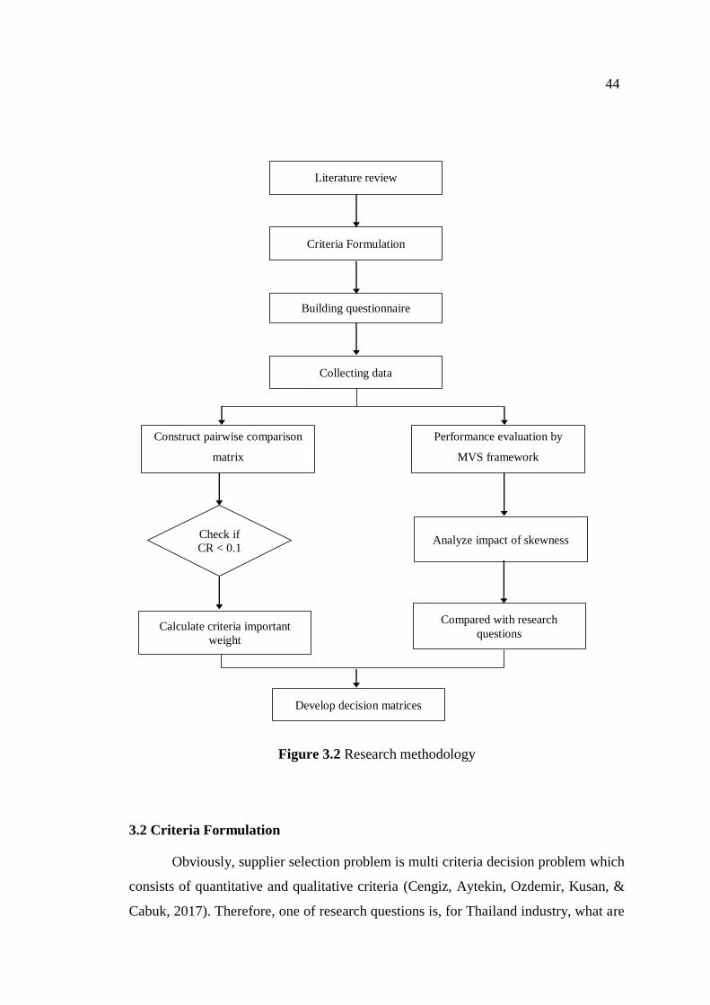
44
Figure 3.2 Research methodology
3.2 Criteria Formulation
Obviously, supplier selection problem is multi criteria decision problem which
consists of quantitative and qualitative criteria (Cengiz, Aytekin, Ozdemir, Kusan, &
Cabuk, 2017). Therefore, one of research questions is, for Thailand industry, what are
Check if
CR < 0.1
Construct pairwise comparison
matrix
Literature review
Building questionnaire
Performance evaluation by
MVS framework
Develop decision matrices
Collecting data
Criteria Formulation
Compared with research
questions Calculate criteria important
weight
Analyze impact of skewness
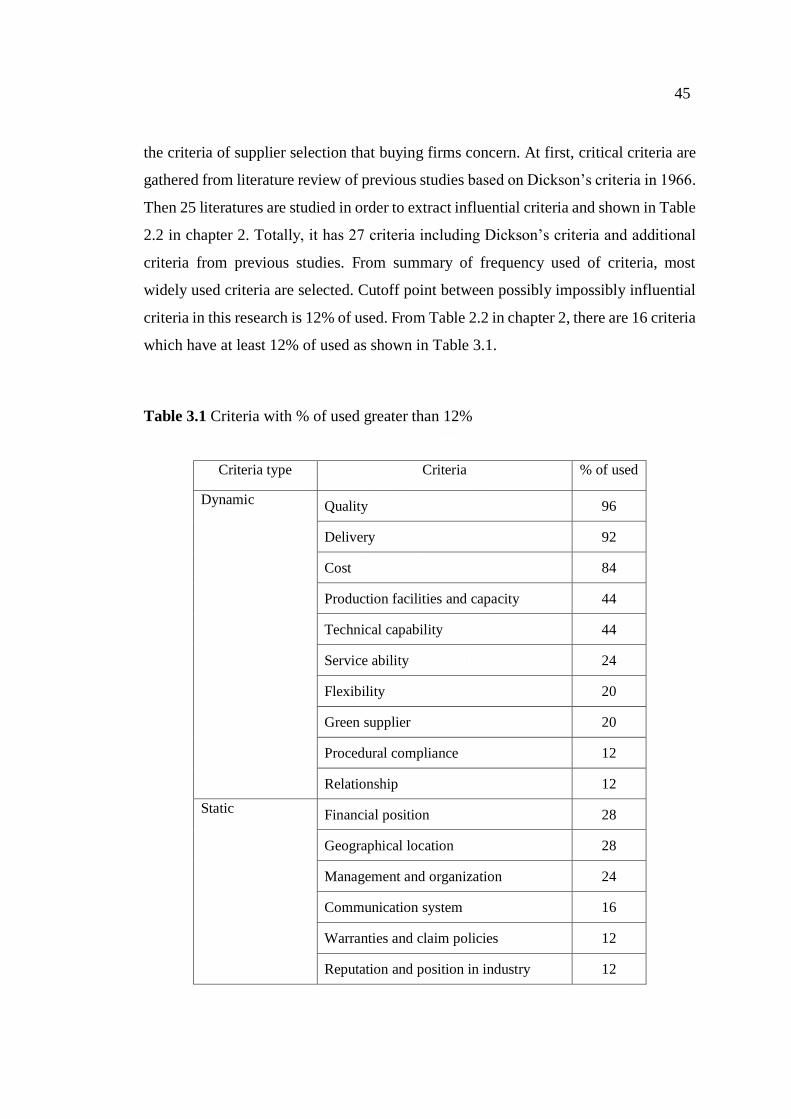
45
the criteria of supplier selection that buying firms concern. At first, critical criteria are
gathered from literature review of previous studies based on Dickson’s criteria in 1966.
Then 25 literatures are studied in order to extract influential criteria and shown in Table
2.2 in chapter 2. Totally, it has 27 criteria including Dickson’s criteria and additional
criteria from previous studies. From summary of frequency used of criteria, most
widely used criteria are selected. Cutoff point between possibly impossibly influential
criteria in this research is 12% of used. From Table 2.2 in chapter 2, there are 16 criteria
which have at least 12% of used as shown in Table 3.1.
Table 3.1 Criteria with % of used greater than 12%
Criteria type Criteria % of used
Dynamic Quality 96
Delivery 92
Cost 84
Production facilities and capacity 44
Technical capability 44
Service ability 24
Flexibility 20
Green supplier 20
Procedural compliance 12
Relationship 12
Static Financial position 28
Geographical location 28
Management and organization 24
Communication system 16
Warranties and claim policies 12
Reputation and position in industry 12

46
To retrieve the final set of criteria, first, criteria are classified into 2 types. First
is dynamic criteria which means criteria that it performance changes all the time.
Another type is static criteria which means criteria with constant performance or criteria
which hardly fluctuated all the time, for example, geographical location. Location
problem is the decision in strategic level. Once the location is selected and facility is
established, it will be used for a long period. Performance of this criteria cannot change
easily, therefore, it is classified as static criteria. This research intends to study
uncertainty in supplier selection, therefore, only dynamic criteria are considered.
Also criteria which have similar characteristics are combined together. The first
pair is production facilities and capacity, and flexibility. Based on their definition,
production facilities and capacity refers to being responsive in terms of order quantity
changing from customer, while flexibility refers to being responsive, not only for order
quantity changing but also changing of design, process or product specification. Both
of them have similarity in characteristics of being responsive. Therefore these 2 criteria
are combined together and renamed as capacity and flexibility in order to reduce the
number of criteria. Another pair is combining between service ability and relationship.
Both of them have similarity of well collaboration from suppliers. Therefore, these 2
criteria are combined together and renamed as collaborative development.
From all of dynamic criteria, they are classified into 5 groups, which are, cost,
delivery, quality, green supplier, and others which comprises of the left criteria as
shown in Figure 3.3.
Cost
Delivery
Quality
Green supplier Others
Capacity and flexibility
Technical capability
Collaborative
development
Figure 3.3 Main criteria

47
After main criteria are set, each main criteria are divided into sub-criteria in
order to evaluate supplier performance in deeper details. Figure 3.4 illustrates all main
criteria as well as sub criteria in each main group.
Figure 3.4 Criteria grouping
Totally there are 6 main criteria with 13 sub-criteria in this research. The
following parts explain each critical criterion and its definition.
1) Cost: One of the most important criteria for supplier selection is cost which
means the overall expense spending to receive product from supplier. It has 2 sub-
criteria:
- Price which means the total price offered from supplier.
- Other cost which means the additional cost other than product price, such as
transportation cost, operating cost.
2) Delivery: This criterion means ability of supplier to provide product to
buyer or manufacturer. In nowadays business environment which tends to compete with
rivals by improving ability to be able to meet customer demands in shorter time,
especially in electronics industry, supplier delivery performance has much effect to
manufacturer’s performance. It has 2 sub-criteria:
Cost
•Price
•Other cost
Delivery
•Lead time
•On-time delivery
Quality
•Product quality and reliability
•Continuous improvement ability
Supplier condition & relationship
•Capacity and flexibility
•Technical capability
• Collaborative development
Green supplier
•Green manufacturing process
•Green product and design
Supplier risk
•Natural risk
•Human risk

48
- Lead time which means the time period used between when placing order to
supplier until receiving.
- On-time delivery means the delivery performance of supplier to fulfill
ordered quantity to manufacturer in the expected time by customer.
3) Quality: Together with cost and delivery, one of the basic supplier’s
requirements is quality of product as well as reliability. This main criterion has 2 sub-
criteria:
- Product quality and reliability means the quality of product which meets
buying firm’s specification and supplier reliability and consistency of
product quality. The performance of this criterion can be measured by return
rate.
- Continuous improvement ability, this sub-criterion is about effort and ability
of supplier to increase performance for the future.
4) Supplier condition and relationship: This is a criterion related to
supplier’s current condition affecting to buyer or manufacturer and relationship
between buying firm and supplier which included 4 sub-criteria:
- Capacity and flexibility means ability to produce order from buyer with big
quantity and responsiveness to changing or additional requirement from
buyer, such as product specification, quantity and procedure.
- Technical capability is the technological proficiency of supplier, not only the
current one but also the potential of future technological research and
development (R&D) both of product design and production process.
- Collaborative development is the cooperation from supplier and buying firm
to improve their capability and efficiency in terms of product development
and process development.
5) Green supplier: Nowadays environmental awareness has been growing.
Therefore, one of the main criteria to select supplier is green supplier which is the
consideration of supplier on environment. It is comprises of 2 sub-criteria:
- Green manufacturing process is the awareness and ability of supplier to lower
consumption of resource and reduce impact on environment in production
process.
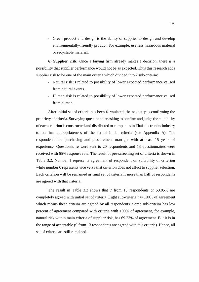
49
- Green product and design is the ability of supplier to design and develop
environmentally-friendly product. For example, use less hazardous material
or recyclable material.
6) Supplier risk: Once a buying firm already makes a decision, there is a
possibility that supplier performance would not be as expected. Thus this research adds
supplier risk to be one of the main criteria which divided into 2 sub-criteria:
- Natural risk is related to possibility of lower expected performance caused
from natural events.
- Human risk is related to possibility of lower expected performance caused
from human.
After initial set of criteria has been formulated, the next step is confirming the
propriety of criteria. Surveying questionnaire asking to confirm and judge the suitability
of each criterion is constructed and distributed to companies in Thai electronics industry
to confirm appropriateness of the set of initial criteria (see Appendix A). The
respondents are purchasing and procurement manager with at least 15 years of
experience. Questionnaire were sent to 20 respondents and 13 questionnaires were
received with 65% response rate. The result of pre-screening set of criteria is shown in
Table 3.2. Number 1 represents agreement of respondent on suitability of criterion
while number 0 represents vice versa that criterion does not affect to supplier selection.
Each criterion will be remained as final set of criteria if more than half of respondents
are agreed with that criteria.
The result in Table 3.2 shows that 7 from 13 respondents or 53.85% are
completely agreed with initial set of criteria. Eight sub-criteria has 100% of agreement
which means these criteria are agreed by all respondents. Some sub-criteria has low
percent of agreement compared with criteria with 100% of agreement, for example,
natural risk within main criteria of supplier risk, has 69.23% of agreement. But it is in
the range of acceptable (9 from 13 respondents are agreed with this criteria). Hence, all
set of criteria are still remained.
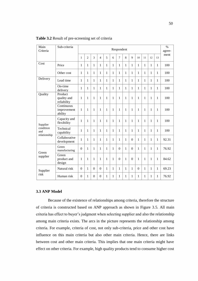
50
Table 3.2 Result of pre-screening set of criteria
Main
Criteria
Sub-criteria Respondent
%
agree-
ment 1 2 3 4 5 6 7 8 9 10 11 12 13
Cost Price 1 1 1 1 1 1 1 1 1 1 1 1 1 100
Other cost 1 1 1 1 1 1 1 1 1 1 1 1 1 100
Delivery Lead time 1 1 1 1 1 1 1 1 1 1 1 1 1 100
On-time
delivery 1 1 1 1 1 1 1 1 1 1 1 1 1 100
Quality Product
quality and
reliability
1 1 1 1 1 1 1 1 1 1 1 1 1 100
Continuous
improvement
ability
1 1 1 1 1 1 1 1 1 1 1 1 1 100
Supplier
condition
and
relationship
Capacity and
flexibility 1 1 1 1 1 1 1 1 1 1 1 1 1 100
Technical
capability 1 1 1 1 1 1 1 1 1 1 1 1 1 100
Collaborative
development 1 1 1 1 1 1 1 1 0 1 1 1 1 92.31
Green
supplier
Green
manufacturing 0 1 1 1 1 1 0 1 0 1 1 1 1 76.92
Green
product and
design
1 1 1 1 1 1 0 1 0 1 1 1 1 84.62
Supplier
risk
Natural risk 0 1 0 0 1 1 1 1 1 0 1 1 1 69.23
Human risk 0 1 0 0 1 1 1 1 1 1 1 1 1 76.92
3.3 ANP Model
Because of the existence of relationships among criteria, therefore the structure
of criteria is constructed based on ANP approach as shown in Figure 3.5. All main
criteria has effect to buyer’s judgment when selecting supplier and also the relationship
among main criteria exists. The arcs in the picture represents the relationship among
criteria. For example, criteria of cost, not only sub-criteria, price and other cost have
influence on this main criteria but also other main criteria. Hence, there are links
between cost and other main criteria. This implies that one main criteria might have
effect on other criteria. For example, high quality products tend to consume higher cost
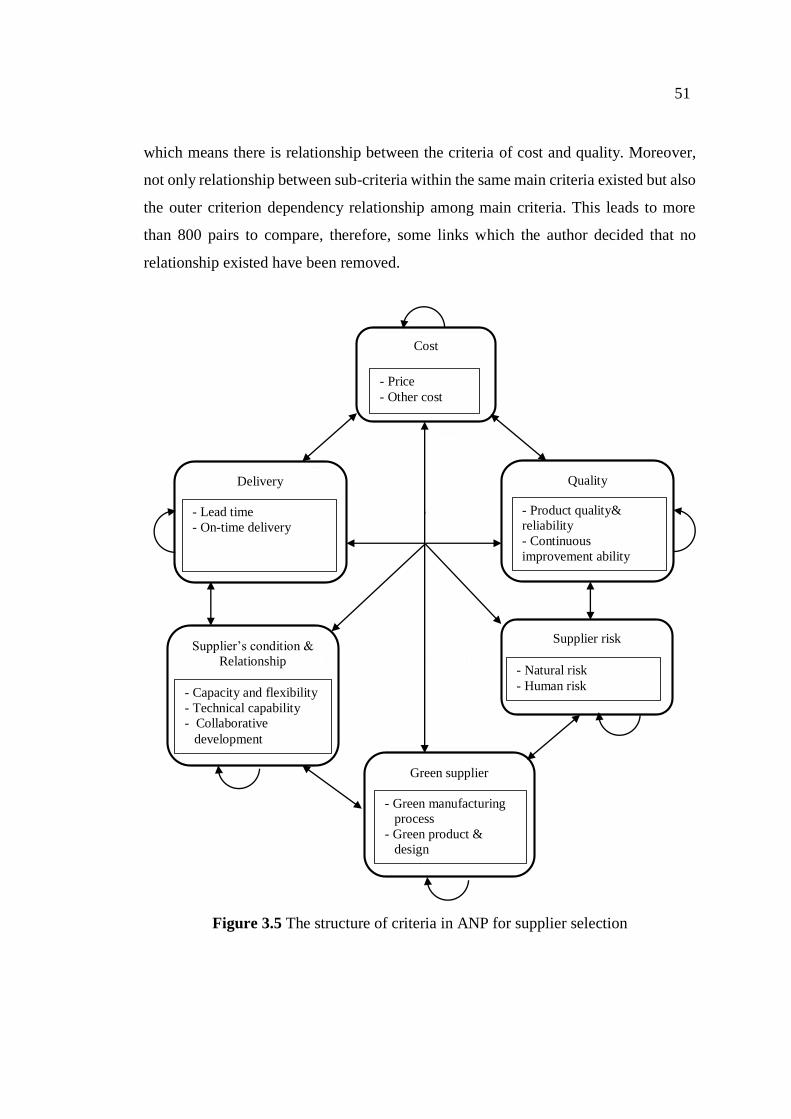
51
which means there is relationship between the criteria of cost and quality. Moreover,
not only relationship between sub-criteria within the same main criteria existed but also
the outer criterion dependency relationship among main criteria. This leads to more
than 800 pairs to compare, therefore, some links which the author decided that no
relationship existed have been removed.
Figure 3.5 The structure of criteria in ANP for supplier selection
Cost
Quality Delivery
Supplier’s condition &
Relationship
Supplier risk
- Price
- Other cost
- Lead time
- On-time delivery
- Product quality&
reliability
- Continuous
improvement ability
- Capacity and flexibility
- Technical capability
- Collaborative
development
- Natural risk
- Human risk
Green supplier
- Green manufacturing
process
- Green product &
design

52
3.4 Building Questionnaire
After the set of criteria is confirmed by experts, the questionnaire is asking about
criteria weight and performance evaluation is constructed (see appendix B).
Questionnaire is separated into 2 main sections. First section is used for criteria
weighting, another section is used for performance evaluating.
3.4.1 Design of Questionnaire: Section 1
For the first section, questionnaire is designed to ask the respondents to compare
a given pair of criteria followed Saaty’s rating scale (1-9) as follows:
1-Equal importance One criteria will influence 1 times more
on a given element than the other does.
2: Equal to moderate importance One criteria will influence 2 times more
on a given element than the other does.
3: Moderate importance One criteria will influence 3 times more
on a given element than the other does.
4: Moderate to strong importance One criteria will influence 4 times more
on a given element than the other does.
5: Strong importance One criteria will influence 5 times more
on a given element than the other does.
6: Strong to very strong importance One criteria will influence 6 times more
on a given element than the other does.
7: Very strong importance One criteria will influence 7 times more
on a given element than the other does.
8: Very strong to extreme importance One criteria will influence 8 times more
on a given element than the other does.
9: Extreme importance One criteria will influence 9 times more
on a given element than the other does.
In this section, questions are divided into 5 parts based on the level of preference
structure, such as, level of relative importance among all main criteria by assuming
53
criteria are independent, level relative importance among main criteria by assuming
interrelation among criteria, etc. The structure of questionnaire can be explained as
follows:
Let C1: cost criteria
C2: delivery criteria
C3: quality criteria
C4: supplier’s condition and relationship criteria
C5: green supplier criteria
C6: supplier risk criteria
Part 1: This part is to measure the relative importance among all main criteria
on supplier selection by assuming existence of dependency relationship as illustrated in
Figure 3.6.
Figure 3. 6 The comparison of relative importance among all main criteria on
supplier selection
Part 2: This part is to measure the relative importance among main criteria by
assuming interrelation among main criteria. To collect the data for this part, respondent
will be asked to judge the relative influence between each pair of main criteria on the
specific main criteria as shown in Figure 3.7.
Supplier Selection
C1 C2 C3 C4 C5 C6
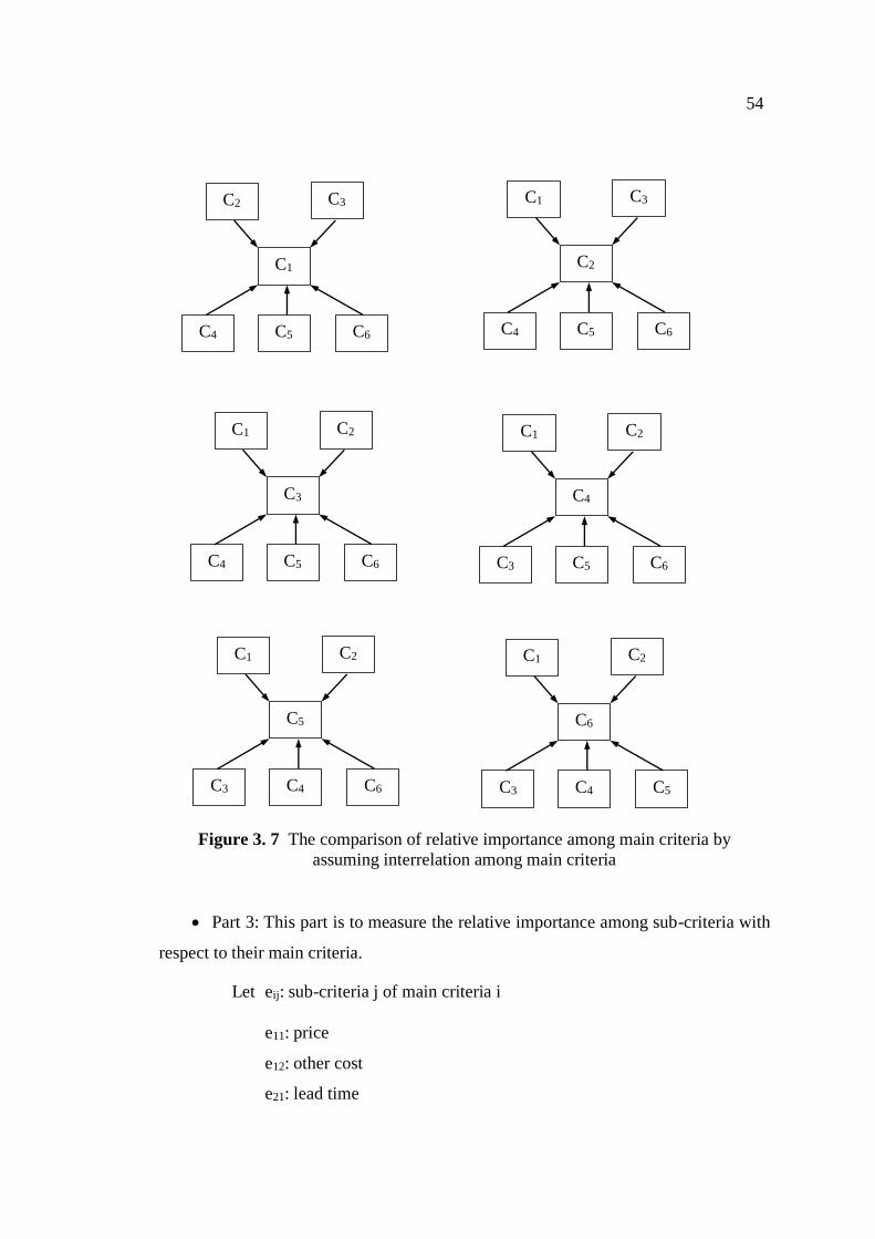
54
Figure 3. 7 The comparison of relative importance among main criteria by
assuming interrelation among main criteria
Part 3: This part is to measure the relative importance among sub-criteria with
respect to their main criteria.
Let eij: sub-criteria j of main criteria i
e11: price
e12: other cost
e21: lead time
C1
C2 C3
C6 C4 C5
C2
C1 C3
C6 C4 C5
C3
C1 C2
C6 C4 C5
C4
C1 C2
C6 C3 C5
C5
C1 C2
C6 C3 C4
C6
C1 C2
C5 C3 C4
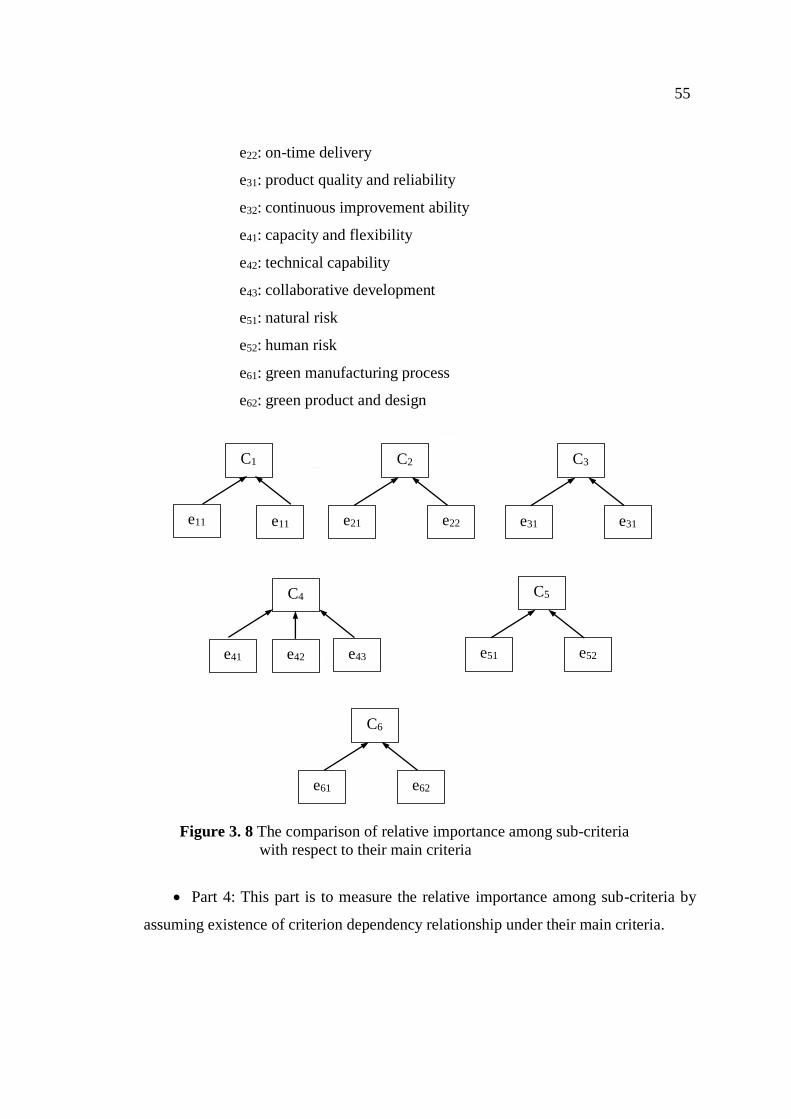
55
e22: on-time delivery
e31: product quality and reliability
e32: continuous improvement ability
e41: capacity and flexibility
e42: technical capability
e43: collaborative development
e51: natural risk
e52: human risk
e61: green manufacturing process
e62: green product and design
Figure 3. 8 The comparison of relative importance among sub-criteria
with respect to their main criteria
Part 4: This part is to measure the relative importance among sub-criteria by
assuming existence of criterion dependency relationship under their main criteria.
C1
e11
C2
e21 e22
C3
e31 e31
C4
e41 e42 e43
C5
e51 e52
C6
e61 e62
e11
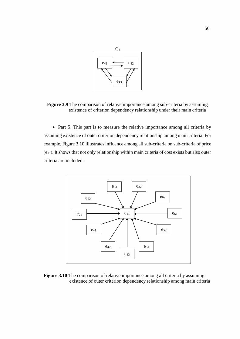
56
Figure 3.9 The comparison of relative importance among sub-criteria by assuming
existence of criterion dependency relationship under their main criteria
Part 5: This part is to measure the relative importance among all criteria by
assuming existence of outer criterion dependency relationship among main criteria. For
example, Figure 3.10 illustrates influence among all sub-criteria on sub-criteria of price
(e11). It shows that not only relationship within main criteria of cost exists but also outer
criteria are included.
Figure 3.10 The comparison of relative importance among all criteria by assuming
existence of outer criterion dependency relationship among main criteria
e41 e42
C4
e43
e11 e21
e22
e31 e32
e41
e42
e43
e51
e52
e61
e62
57
3.4.2 Design of Questionnaire: Section 2
The second section of questionnaire is designed to ask the respondents (i.e.
purchasing manager) to evaluate historical performance of potential suppliers for each
criteria. In questionnaire, respondent will be asked to evaluate between two current
suppliers, namely supplier A and supplier B. The questions in this section is separated
into two parts. In part 1, the respondent will be asked to select current two suppliers
who can provide same material or part. One is supplier who has first priority to be
selected, in other words, this represents good supplier. Another one is supplier who
would be the last choice to be selected or bad suppliers which express bad supplier. In
part 2, the respondent will be asked to rate performance of each supplier based on each
criteria. Performance will be measured in three characteristics:
1. Performance Efficiency refers to the expected of efficiency of supplier
measured by mean.
2. Performance Stability refers to standard deviation. Because good supplier
should provide constant performance or standard deviation of supplier’s performance
should be low.
3. Performance Tendency refers to skewness. As mentioned earlier, it does not
mean that supplier with no tendency to differ from average efficiency or not fluctuate
is good. Hence, this performance reflect the asymmetrical direction of efficiency which
measured by skewness.
Asking respondent to evaluate suppliers’ standard deviation and skewness is not
easy. In order to obtain these two characteristics, the respondent will be asked to
evaluate lower and upper bound of performance, i.e. minimum and maximum level of
criterion performance and most often occurred performance, i.e. mode which provided
by each supplier. The standard deviation will be calculated using the estimation of range,
i.e. the difference between maximum and minimum level of performance obtained from
questionnaire. This estimation is proved and proposed by Hozo, Djulbegovic, and Hozo
(2005) and it is showed in equation 3.1. The skewness will be calculated using
pearson’s coefficient of skewness which is estimating skewness by mean and mode
obtained from questionnaire as shown in equation 3.2.
58
6
RangeSD (3.1)
SD
modeXSk
(3.2)
Where SD is standard deviation
Range is difference between lowest and highest of the range
Sk is skewness
Mode is most often occurred performance
3.5 Determining Target Group and Data Collecting
Although this research has set manufacturers in electronics industry as target
group. But there is a large number of manufacturers in this industry. Also,
characteristics of manufacturers in this industry are very heterogeneous due to many
types of products and manufacturers. A method that could be used to classified
manufacturing types is using TSIC. TSIC is a 5-digit-code generated by Department of
Industrial Works, Ministry of Industry. Based on TSIC, manufacturing companies in
electronics industry can be grouped into 7 types which are;
1. Electronic devices, part and coil
2. Computer storage equipment
3. Lighting equipment
4. Transformer, uninterrupted power supply, battery, electric wire
5. Computer part, Print circuit board, electronic mainboard
6. Home Electrical machine
7. VDO recorder, camera, lens
After classifying all manufacturers in electronics industry based on TSIC code,
each type still has large number of manufacturer. Then manufacturers in each type are
classified based on size of company using Small and Medium Enterprises Promotion
Act, B.E. 2543. Based on the rule of this promotion act, size of manufacturers can be
classified into 3 categories, small, medium and large enterprise by these following rules;

59
- Small-size-manufacture (S): number of employees is not greater than 50
employees or asset value is not greater than 50 million baht.
- Medium-size-manufacturer (M): number of employees is between 51-200
employees or asset value between 50-200 million baht.
- Large-size-manufacturer (L): number of employees is greater than 200
employees or asset value is greater than 200 million baht.
Finally, manufacturers in electronics industry can be re-group based on its
character and product type (manufacturer type based on TSIC) as well as size of
company (based on Promotion Act) as shown in Table 3.3.
Table 3. 3 Clustering of Thailand’s electronics industry
Types of manufacturer Size of company
S M L
Electronic devices, part and coil 152 28 7
Computer storage equipment 25 4 2
Lighting equipment 50 24 9
Transformer, uninterrupted power
supply, battery, electric wire
270 138 48
Computer part, Print circuit board,
electronic mainboard
22 16 34
Home Electrical machine
- Stereo, Television 502 177 162
- Refrigerator, Fan, washing
machine, air-conditioner
493 173 78
- Other home electrical machines 23 1 1
VDO recorder, camera, lens 11 12 12
Total 1548 573 353
Source: Department of Industrial Works, Ministry of Industry (31 Jan 2016)
60
In this research, home electrical machine which is the nearest tier to end
customer has been selected as target group. Because suppliers of this manufacturing
type are companies who produce, for example, electronics device, motor, coil, electric
wire, which are still in electronics industry. But if electronics devices are selected as
target group, suppliers of this manufacturing type fall on other industry, such as, plastic
industry, steel industry, rubber industry. Home electrical machine is selected in order
to avoid such circumstance. Also only M and L-size-manufacture are selected as target
group. Because of small manufacturers are possibly to have no standard and no system,
the result may has much variance if small-sized manufacturers are including. Hence,
total population size is 592 companies.

61
CHAPTER 4
RESULT ANALYSIS
This chapter presents result of data analysis obtained from the survey. First,
summary of respondents are presented, follows by criteria important weight and result
of performance evaluating. Then the skewness effect is analyzed. Finally, decision
matrix of supplier selection is proposed.
4.1 Summary of Respondents
After set of criteria were formulated and questionnaire was constructed, then
the data survey was begin as mention in precious chapter. To determine sample size,
this research refers to sample size from previous researches which applied similar
method, i.e. MCDM techniques. Table 4.1 presents number of sample size from
previous researches.
Table 4. 1 Number of sample size from previous researches
No. Year Authors Sample size
1 1998 Verma & Pullman 58
2 1999 Yahha & Kingsman 16
3 2005 Lie & Hai 60
4 2007 Gurpina 16
5 2012 Bruno et al. 20
6 2014 Dargi et al. 4
7 2014 Lima et al. 3
From Table 4.1, the maximum sample size from previous studies are 60. Therefore, this research set minimum sample size required equals to 60 sample sizes.
After the sample size is determined, then the survey is conducted by two ways. One is
face-to-face interview, another one is questionnaire distribution.
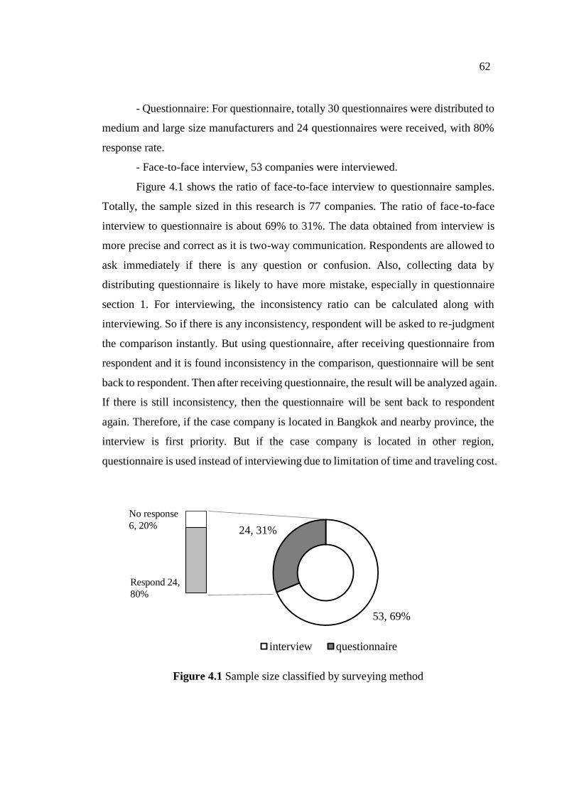
62
- Questionnaire: For questionnaire, totally 30 questionnaires were distributed to
medium and large size manufacturers and 24 questionnaires were received, with 80%
response rate.
- Face-to-face interview, 53 companies were interviewed.
Figure 4.1 shows the ratio of face-to-face interview to questionnaire samples.
Totally, the sample sized in this research is 77 companies. The ratio of face-to-face
interview to questionnaire is about 69% to 31%. The data obtained from interview is
more precise and correct as it is two-way communication. Respondents are allowed to
ask immediately if there is any question or confusion. Also, collecting data by
distributing questionnaire is likely to have more mistake, especially in questionnaire
section 1. For interviewing, the inconsistency ratio can be calculated along with
interviewing. So if there is any inconsistency, respondent will be asked to re-judgment
the comparison instantly. But using questionnaire, after receiving questionnaire from
respondent and it is found inconsistency in the comparison, questionnaire will be sent
back to respondent. Then after receiving questionnaire, the result will be analyzed again.
If there is still inconsistency, then the questionnaire will be sent back to respondent
again. Therefore, if the case company is located in Bangkok and nearby province, the
interview is first priority. But if the case company is located in other region,
questionnaire is used instead of interviewing due to limitation of time and traveling cost.
Figure 4.1 Sample size classified by surveying method
53, 69%
24, 31%
interview questionnaire
No response
6, 20%
Respond 24,
80%
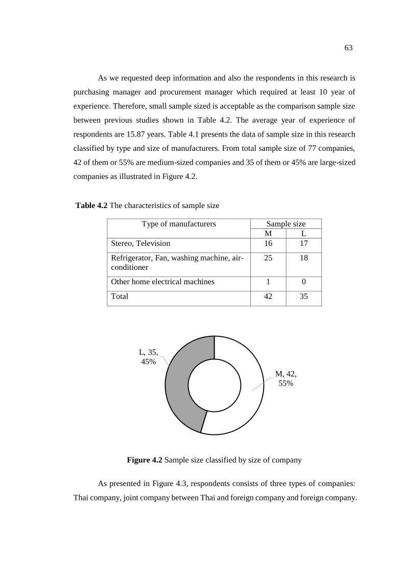
63
As we requested deep information and also the respondents in this research is
purchasing manager and procurement manager which required at least 10 year of
experience. Therefore, small sample sized is acceptable as the comparison sample size
between previous studies shown in Table 4.2. The average year of experience of
respondents are 15.87 years. Table 4.1 presents the data of sample size in this research
classified by type and size of manufacturers. From total sample size of 77 companies,
42 of them or 55% are medium-sized companies and 35 of them or 45% are large-sized
companies as illustrated in Figure 4.2.
Table 4.2 The characteristics of sample size
Type of manufacturers Sample size
M L
Stereo, Television 16 17
Refrigerator, Fan, washing machine, air-
conditioner
25 18
Other home electrical machines 1 0
Total 42 35
Figure 4.2 Sample size classified by size of company
As presented in Figure 4.3, respondents consists of three types of companies:
Thai company, joint company between Thai and foreign company and foreign company.
M, 42,
55%
L, 35,
45%

64
Figure 4.3 Sample size classified by types of company
Purchasing and procurement experts from each company was interviewed or
requested to fill out the questionnaire asking to evaluate and compare performance
between key supplier which is recognized as supplier with good performance and
unfavorable supplier which is recognized as bad supplier who would be the first and
the last choice to be considered when buying, respectively, in order to analyze whether
it has different performance perspective between these two suppliers, especially
skewness.
4.2 Importance of Criteria
4.2.1 Overall Criteria Importance
In this research, ANP approach is used to analyze important weight of criteria.
Compare among main six criteria or dimension, supplier condition and relationship is
the most important criteria, follows by delivery, cost, quality, supplier risk, and green
supplier respectively. It is surprisingly that CQD (Cost; Quality; Delivery) are not the
top-3 criteria as people always thought. But manufacturers in Thai electronics industry
concern most about supplier condition and relationship which mostly rely on the
flexibility and technical capability. Because of competitive environment tends to
become more severe, more customization and more rapid, competition becomes more
intense. Then supplier must be able to meet customers’ need rapidly.
Thai ,
19, 25%
Joint,
23, 30%
Foreign,
35, 45%
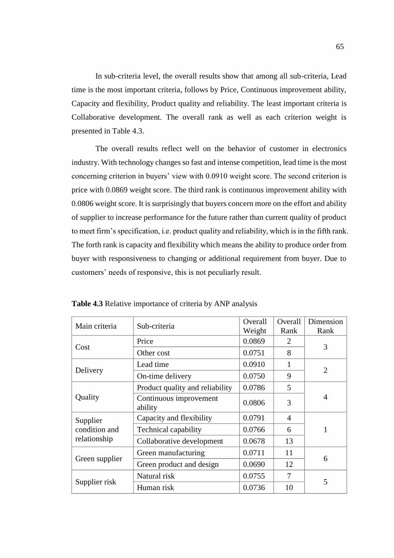
65
In sub-criteria level, the overall results show that among all sub-criteria, Lead
time is the most important criteria, follows by Price, Continuous improvement ability,
Capacity and flexibility, Product quality and reliability. The least important criteria is
Collaborative development. The overall rank as well as each criterion weight is
presented in Table 4.3.
The overall results reflect well on the behavior of customer in electronics
industry. With technology changes so fast and intense competition, lead time is the most
concerning criterion in buyers’ view with 0.0910 weight score. The second criterion is
price with 0.0869 weight score. The third rank is continuous improvement ability with
0.0806 weight score. It is surprisingly that buyers concern more on the effort and ability
of supplier to increase performance for the future rather than current quality of product
to meet firm’s specification, i.e. product quality and reliability, which is in the fifth rank.
The forth rank is capacity and flexibility which means the ability to produce order from
buyer with responsiveness to changing or additional requirement from buyer. Due to
customers’ needs of responsive, this is not peculiarly result.
Table 4.3 Relative importance of criteria by ANP analysis
Main criteria Sub-criteria Overall
Weight
Overall
Rank
Dimension
Rank
Cost Price 0.0869 2
3 Other cost 0.0751 8
Delivery Lead time 0.0910 1
2 On-time delivery 0.0750 9
Quality
Product quality and reliability 0.0786 5
4 Continuous improvement
ability 0.0806 3
Supplier
condition and
relationship
Capacity and flexibility 0.0791 4
1 Technical capability 0.0766 6
Collaborative development 0.0678 13
Green supplier Green manufacturing 0.0711 11
6 Green product and design 0.0690 12
Supplier risk Natural risk 0.0755 7
5 Human risk 0.0736 10
66
An issue should not overlook is, even though people always talk about being
environmental friendly, and raise awareness of green issue, in fact buyers seem not to
care for this criteria as green supplier is the least important main criteria. Also, both of
sub-criteria of green supplier are ranked in eleventh and twelfth place.
4.2.2 Criteria Importance Classified by Size of Company
Classified by size of company, important weight of each criterion between
medium and large size company are not much different as shown in Figure 4.4.
However, their criteria rank are slightly different due to their characteristics. For
medium-sized manufacturers, the most affecting criteria on buyers’ decision is price,
follows by lead time, product quality and reliability, continuous improvement ability,
and capacity and flexibility. While the most concerning factor for large-sized
manufacturers is lead time, follows by price, technical capability, continuous
improvement ability, and other cost. The reasons of this difference is, medium-sized
manufacturers have more limited resource than large manufacturers, especially
financial resource. Therefore, price criteria is the most important thing that medium-
sized manufacturers concern while L-sized manufacturers seek for rapid suppliers who
provided short lead time.
Table 4.4 compares rank of criteria importance among medium-sized
manufacturers, large-sized manufacturers, and overall result. From this table, although
important weights of the same criteria are not much different but rankings are slightly
different. The first top-2 important criteria of both sizes are price and lead time, same
as overall rank but different place. While L-sized manufactures concerned much about
technical capability as this sub-criteria is ranked in third place, M-sized manufacturers
concerned about product quality and reliability. This is because L-sized manufacturers
have sufficient resource and power over other manufacturers, so they would want to be
leaders in the industry. To become trendsetters, they need high technical supporting in
terms of designing new product and developing new technology.
About criteria with lowest important weight, bottom-3 criteria which have
lowest important weight of L-sized manufacturers are collaborative development, green

67
manufacturing, green product and design, same as overall ranking. But for M-sized
manufacturers, bottom-3 ranked criteria are collaborative development, green product
and design, and technical capability, which is the remarkable result. While technical
capability is the third ranked criteria that large-sized manufacturers concern but it seems
to have less important to medium-sized manufacturers. This is because the opposite
reason with L-sized manufacturers’. Medium sized manufacturers have less resource
than L-sized, especially financial resource. They do not position themselves to become
leaders in this industry. So they do not required much on high technical support as it
may leads to higher cost.
Table 4.4 Criteria ranking between medium and large-sized manufacturers
Sub-criteria Overall Medium-sized Large-sized
Weight Rank Weight Rank Weight Rank
Price 0.0869 2 0.0858 1 0.0882 2
Other cost 0.0751 8 0.0722 10 0.0784 5
Lead time 0.0910 1 0.0851 2 0.0981 1
On-time delivery 0.0750 9 0.0739 9 0.0764 7
Product quality and
reliability 0.0786 5 0.0822 3 0.0744 8
Continuous
improvement ability 0.0806 3 0.0809 4 0.0804 4
Capacity and flexibility 0.0791 4 0.0800 5 0.0780 6
Technical capability 0.0766 6 0.0719 11 0.0822 3
Collaborative
development 0.0678 13 0.0716 12 0.0632 13
Green manufacturing 0.0711 11 0.0756 7 0.0657 12
Green product and
design 0.0690 12 0.0674 13 0.0710 11
Natural risk 0.0755 7 0.0785 6 0.0718 10
Human risk 0.0736 10 0.0748 8 0.0721 9
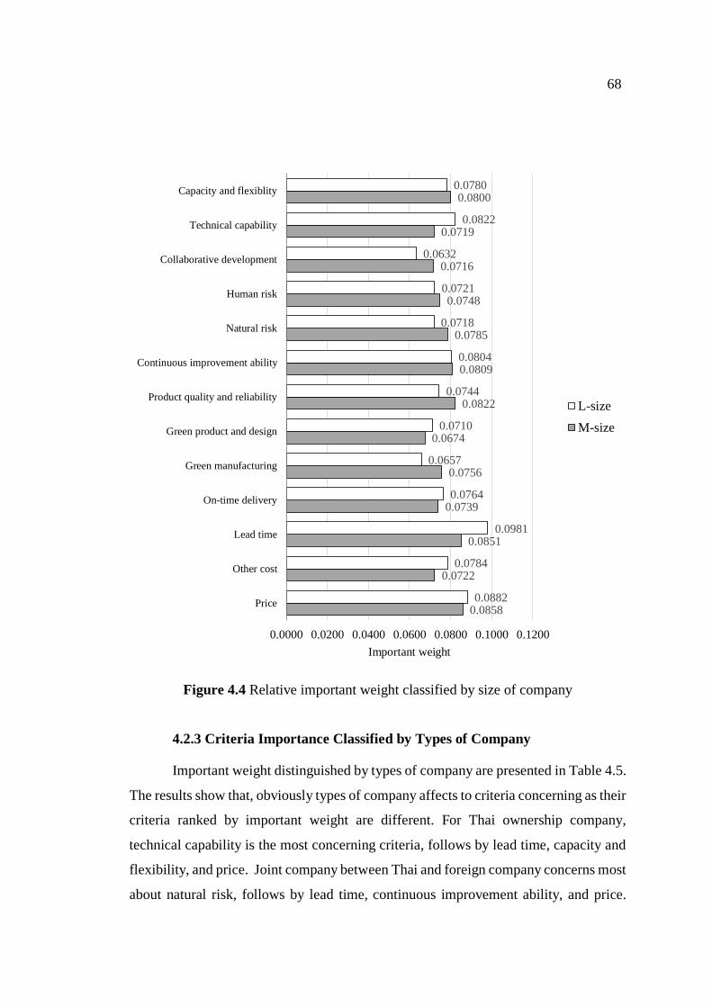
68
Figure 4.4 Relative important weight classified by size of company
4.2.3 Criteria Importance Classified by Types of Company
Important weight distinguished by types of company are presented in Table 4.5.
The results show that, obviously types of company affects to criteria concerning as their
criteria ranked by important weight are different. For Thai ownership company,
technical capability is the most concerning criteria, follows by lead time, capacity and
flexibility, and price. Joint company between Thai and foreign company concerns most
about natural risk, follows by lead time, continuous improvement ability, and price.
0.0858
0.0722
0.0851
0.0739
0.0756
0.0674
0.0822
0.0809
0.0785
0.0748
0.0716
0.0719
0.0800
0.0882
0.0784
0.0981
0.0764
0.0657
0.0710
0.0744
0.0804
0.0718
0.0721
0.0632
0.0822
0.0780
0.0000 0.0200 0.0400 0.0600 0.0800 0.1000 0.1200
Price
Other cost
Lead time
On-time delivery
Green manufacturing
Green product and design
Product quality and reliability
Continuous improvement ability
Natural risk
Human risk
Collaborative development
Technical capability
Capacity and flexiblity
Important weight
L-size
M-size
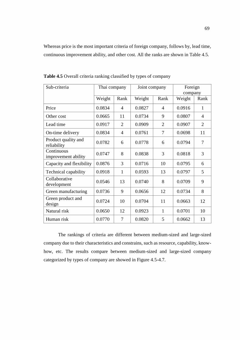
69
Whereas price is the most important criteria of foreign company, follows by, lead time,
continuous improvement ability, and other cost. All the ranks are shown in Table 4.5.
Table 4.5 Overall criteria ranking classified by types of company
Sub-criteria Thai company Joint company Foreign
company
Weight Rank Weight Rank Weight Rank
Price 0.0834 4 0.0827 4 0.0916 1
Other cost 0.0665 11 0.0734 9 0.0807 4
Lead time 0.0917 2 0.0909 2 0.0907 2
On-time delivery 0.0834 4 0.0761 7 0.0698 11
Product quality and
reliability 0.0782 6 0.0778 6 0.0794 7
Continuous
improvement ability 0.0747 8 0.0838 3 0.0818 3
Capacity and flexibility 0.0876 3 0.0716 10 0.0795 6
Technical capability 0.0918 1 0.0593 13 0.0797 5
Collaborative
development 0.0546 13 0.0740 8 0.0709 9
Green manufacturing 0.0736 9 0.0656 12 0.0734 8
Green product and
design 0.0724 10 0.0704 11 0.0663 12
Natural risk 0.0650 12 0.0923 1 0.0701 10
Human risk 0.0770 7 0.0820 5 0.0662 13
The rankings of criteria are different between medium-sized and large-sized
company due to their characteristics and constrains, such as resource, capability, know-
how, etc. The results compare between medium-sized and large-sized company
categorized by types of company are showed in Figure 4.5-4.7.
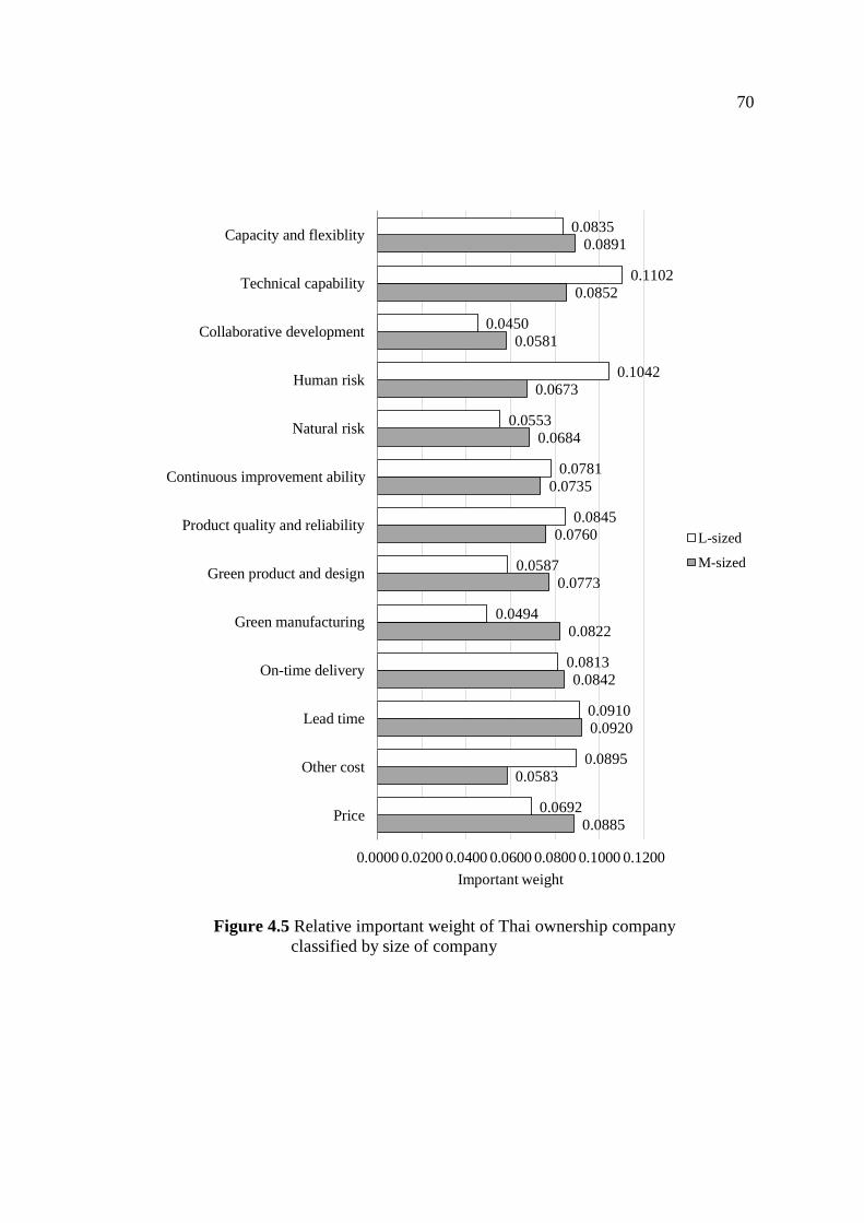
70
Figure 4.5 Relative important weight of Thai ownership company
classified by size of company
0.0885
0.0583
0.0920
0.0842
0.0822
0.0773
0.0760
0.0735
0.0684
0.0673
0.0581
0.0852
0.0891
0.0692
0.0895
0.0910
0.0813
0.0494
0.0587
0.0845
0.0781
0.0553
0.1042
0.0450
0.1102
0.0835
0.0000 0.0200 0.0400 0.0600 0.0800 0.1000 0.1200
Price
Other cost
Lead time
On-time delivery
Green manufacturing
Green product and design
Product quality and reliability
Continuous improvement ability
Natural risk
Human risk
Collaborative development
Technical capability
Capacity and flexiblity
Important weight
L-sized
M-sized
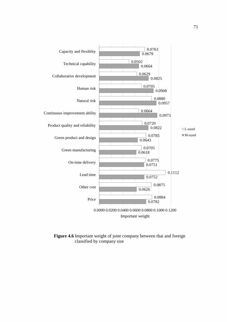
71
Figure 4.6 Important weight of joint company between thai and foreign
classified by company size
0.0782
0.0626
0.0752
0.0751
0.0618
0.0643
0.0822
0.0973
0.0957
0.0908
0.0825
0.0664
0.0679
0.0884
0.0875
0.1112
0.0775
0.0705
0.0785
0.0720
0.0664
0.0880
0.0705
0.0629
0.0502
0.0763
0.0000 0.0200 0.0400 0.0600 0.0800 0.1000 0.1200
Price
Other cost
Lead time
On-time delivery
Green manufacturing
Green product and design
Product quality and reliability
Continuous improvement ability
Natural risk
Human risk
Collaborative development
Technical capability
Capacity and flexiblity
Important weight
L-sized
M-sized

72
Figure 4.7 Relative important weight of foreign company
classified by size of company
4.3 Performance Evaluating
In questionnaire, respondents are asking to select their current suppliers. One is
the first priority supplier which means the most favorable supplier who is the first
priority to be selected. Another one is the alternative supplier who is less priority to be
selected, namely, less priority supplier. The respondents are asked to evaluate
performance based on real data or satisfaction score for objective criteria and subjective
criteria, respectively. The types of criteria are shown in Table 4.6.
0.0900
0.0936
0.0871
0.0633
0.0814
0.0608
0.0879
0.0735
0.0731
0.0679
0.0748
0.0643
0.0820
0.0928
0.0711
0.0934
0.0746
0.0673
0.0704
0.0730
0.0879
0.0679
0.0649
0.0679
0.0913
0.0775
0.0000 0.0200 0.0400 0.0600 0.0800 0.1000
Price
Other cost
Lead time
On-time delivery
Green manufacturing
Green product and design
Product quality and reliability
Continuous improvement ability
Natural risk
Human risk
Collaborative development
Technical capability
Capacity and flexiblity
Important weight
L-sized
M-sized
73
As explanation in Chapter 3 that the performance in this research is measured
into 3 characteristics. Therefore in each criteria, respondent are asked to evaluate
performance of supplier in order to obtain the value of mean, SD, and skewness. But
to obtain the value of SD and skewness is not easy as mentioned earlier. Threrefore, the
question in questionnaire is not directly asked respondents to provide the value of SD
and skewness but after the survey was done, the results from questionnaire are
transformed into 3 perspectives, which are, mean, standard deviation and skewness
using equations showed in chapter 3.
Table 4.6 Types of criteria
Type Sub-criteria Index
Objective Price Actual price
Other cost Actual cost
Lead time Actual lead time
On-time delivery % On-time delivery
Product quality and reliability % Return rate
Subjective Continuous improvement ability Satisfaction score
Capacity and flexibility
Technical capability
Collaborative development
Green manufacturing
Green product and design
Natural risk
Human risk
4.3.1 Coefficient of Variation
The overall results of CV (Coefficient of Variation) categorized by size of
company is presented in Table 4.7. From the results of performance evaluated by
buying manufacturers, although we indicated that in this research performance
perspective is defined into 3 characteristics, 1) efficiency measured by mean, 2)
stability measured by standard deviation, and 3) tendency measured by skewness, only
2 indexes are shown in Table 4.7. CV means coefficient of variation which represents
the ratio between standard deviation to the mean. Hence this statistical measure
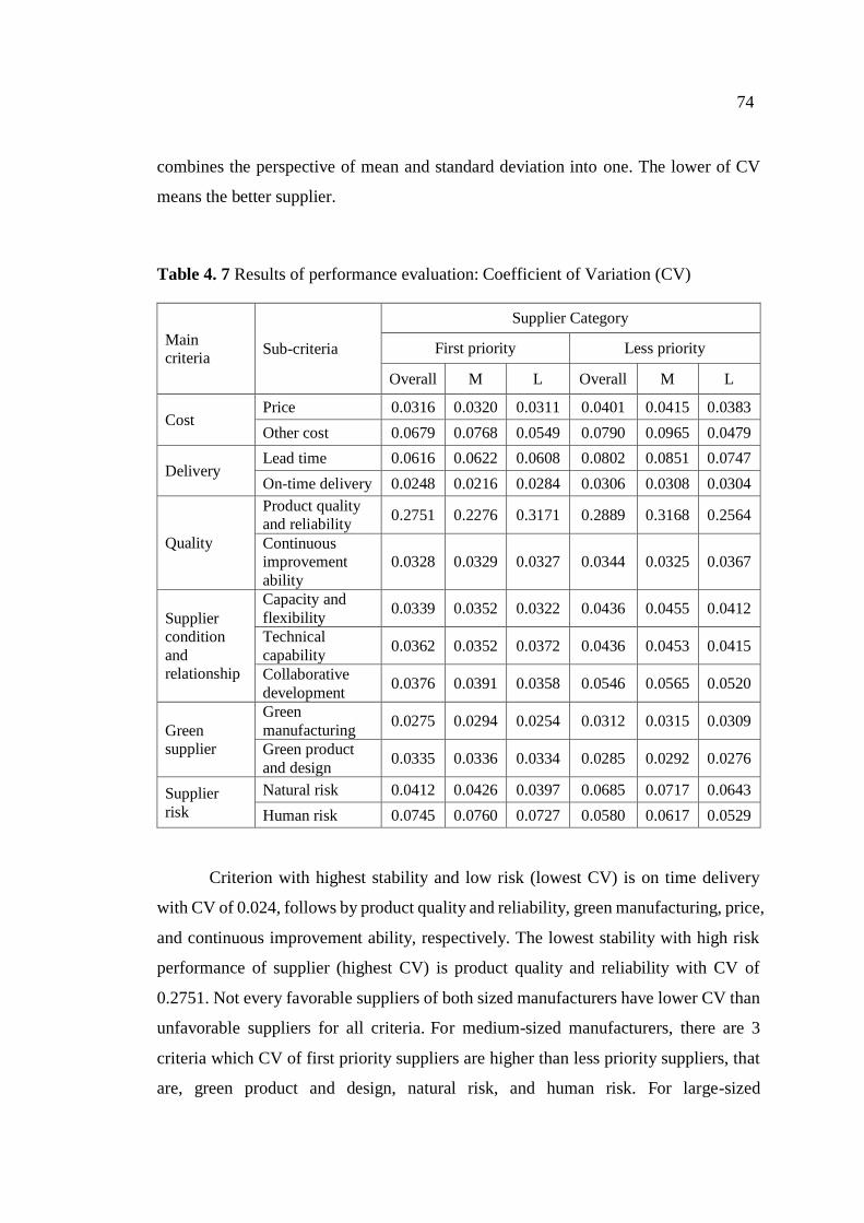
74
combines the perspective of mean and standard deviation into one. The lower of CV
means the better supplier.
Table 4. 7 Results of performance evaluation: Coefficient of Variation (CV)
Main
criteria Sub-criteria
Supplier Category
First priority Less priority
Overall M L Overall M L
Cost Price 0.0316 0.0320 0.0311 0.0401 0.0415 0.0383
Other cost 0.0679 0.0768 0.0549 0.0790 0.0965 0.0479
Delivery Lead time 0.0616 0.0622 0.0608 0.0802 0.0851 0.0747
On-time delivery 0.0248 0.0216 0.0284 0.0306 0.0308 0.0304
Quality
Product quality
and reliability 0.2751 0.2276 0.3171 0.2889 0.3168 0.2564
Continuous
improvement
ability
0.0328 0.0329 0.0327 0.0344 0.0325 0.0367
Supplier
condition
and
relationship
Capacity and
flexibility 0.0339 0.0352 0.0322 0.0436 0.0455 0.0412
Technical
capability 0.0362 0.0352 0.0372 0.0436 0.0453 0.0415
Collaborative
development 0.0376 0.0391 0.0358 0.0546 0.0565 0.0520
Green
supplier
Green
manufacturing 0.0275 0.0294 0.0254 0.0312 0.0315 0.0309
Green product
and design 0.0335 0.0336 0.0334 0.0285 0.0292 0.0276
Supplier
risk
Natural risk 0.0412 0.0426 0.0397 0.0685 0.0717 0.0643
Human risk 0.0745 0.0760 0.0727 0.0580 0.0617 0.0529
Criterion with highest stability and low risk (lowest CV) is on time delivery
with CV of 0.024, follows by product quality and reliability, green manufacturing, price,
and continuous improvement ability, respectively. The lowest stability with high risk
performance of supplier (highest CV) is product quality and reliability with CV of
0.2751. Not every favorable suppliers of both sized manufacturers have lower CV than
unfavorable suppliers for all criteria. For medium-sized manufacturers, there are 3
criteria which CV of first priority suppliers are higher than less priority suppliers, that
are, green product and design, natural risk, and human risk. For large-sized
75
manufacturers, there are 5 criteria, which are, other cost, product quality and reliability,
green product and design, natural risk, and human risk. However, the influence of these
criteria are not much high compared with criteria which first priority suppliers have
lower CV judged by their important weight.
In the next section, each main criteria will be discussed one by one based on the
results in Table 4.7.
1. Cost: The first sub-criteria to discuss in this dimension is price. For both of
medium and large-sized buyers, first priority and less priority suppliers have similar
variation, i.e. both CV are close to each other. However, less priority suppliers have a
little higher CV. This means, based on buyers’ opinion, first priority supplier should
provide more stable performance. Also first priority suppliers of large-sized company
seems to have more stable, i.e. less variation, performance than less priority suppliers.
Compare to price, other cost is more unstable than price. Because of many external
factors affecting to other cost, it is hard for supplier to control these factors, such as,
fuel surcharge, foreign exchange rate which fluctuated throughout the time. First
priority suppliers of medium-sized have lower variation than less priority suppliers
while suppliers of large-sized have a little bit higher variation. However, the overall CV
shows that first priority suppliers have lower CV, i.e. higher stability than less priority
suppliers.
2. Delivery: Despite many criteria involved in supplier selection, we cannot
deny that one of the most important criteria at all time is lead time, especially in current
business era of high responsive. From Table 4.7, it can be seen that first priofity supplier
has lower CV than less priority supplier. This means buyers would select supplier with
higher stability and low variance because it is easier to make a schedule plan. This is
also true with on-time delivery. Even there is not much different between CV of first
priority and less prioity suppliers, nevertheless, first priority suppliers have lower CV.
Also, the results show that on-time delivery seems to have lower variance and higher
stability than lead time as its CV is lower.
3. Quality: For the sub-criteria of product quality and reliability, CV of first
priority and less priority supplier are not much different compared with sub-criteria of
continuous improvement ability. Even first priority suppliers of medium-sized

76
manufacturers have a little higher CV than less priority suppliers, 0.0329 and 0.0325,
respectively, the difference is very narrow so it can be conclude that their CV is not
different. First priority suppliers of large-sized manufacturers have higher variation, i.e.
CV of product quality and reliability than less priority suppliers. But this sub-criteria
has merely moderate importance based on the judgment of large-sized buyers as
important weight shown in Table 4.4. Also their CV is not much different.
4. Supplier Condition and Relationship: This main criteria is the most important
criteria which has highest weight important compared with other main criteria. For all
3 sub-criteria in this dimension, although first priority and less priority suppliers have
not much different CV, it is obvious that les priority suppliers of both sizes still have
higher CV than first priority suppliesrs.
5. Green Supplier: For green manufacturing, the result is in accordance with the
assumption that first priority suppliers should be more stable than less priority suppliers.
However, their CV are not much different. Differ from green manufacturing, for green
product and design, first priority suppliers have a little higher value of CV than less
priority suppliers. One of the main reason is the insignificance of green supplier criteria.
From the result of criteria important weight, green manufacturing and green product
and design are in eleventh and twelfth rank, respectively. This induces suppliers not to
regard much with improving green efficiency because buyers have low concern about
this criteria.
6. Supplier Risk: From Table 4.7, both of medium and large-sized
manufacturers have higher CV on first priority suppliers rather than less priority
suppliers in criteria of human risk. But compared with natural risk, the difference of
CV for natural risk is much higher with lower CV on first priority suppliers. Therefore,
we may say that, first priority suppliers tend to have higher stability than less priority
suppliers for the overall result of this main criteria. However, human risk seems to have
more variation than natural risk for both sizes.
In summary, suppliers of medium-sized manufacturers tend to have higher CV
than large-sized manufactures. This is because of medium-sized buyers are likely to
have weaker power compared with large-sized buyers. Due to their quantity purchased,
resources and financial statement, they have fewer options than large buyers. Therefore,
77
even their first priority suppliers tends to have lower stability compared with large-
sized companies’ suppliers.
4.3.2 Skewness
Based on the direction of skewness, there are 2 types of performance. One is
performance with preference of negative skewness or the higher of performance index,
the better efficiency, such as %on-time delivery. In this case, buyers would expect
greater value of performance or prefer suppliers who have left-skewed performance.
Conversely, another one is performance with preference of positive skewness or the
lower of performance index, the better efficiency, such as cost and lead time. In this
case, buyers would expect lower value of performance or prefer right-skewed rather
than left-skewed performance. According to set of criteria in this research, each type of
skewness preference is shown as followings:
Type I: Positive skewness preference or right-skewed performance: Buyers
prefer lower value of performance than expectation. In other words, lower value means
better performance. There are 4 criteria in this type, namely, price, other cost, lead time,
and product quality and reliability.
Type II: Negative skewness preference or left-skewed performance: Buyers
prefer higher value of performance than expectation which means greater value, better
performance. The rest of criteria are in this type, which are, on-time delivery,
continuous improvement ability, capacity and flexibility, technical capability,
collaborative development, green manufacturing, green product and design, natural risk,
human risk.
Table 4.8 presents the result of skewness evaluation. For type I performance, 3
of 4 criteria in this type have skewed performance as expected. For example, criteria of
lead time, first priority suppliers for both of medium and large-sized have shorter lead
time than buyers’ expectation, i.e., average lead time as their skewness is positive value.
This means in buyers’ perspective, favorable supplier is supplier who is able to provide
product in shorter time than promised lead time. In contrast to first priority suppliers,
suppliers with less priority have left-skewed performance which means most likely they
provide product with longer lead time than promised lead time.

78
Table 4.8 Results of performance evaluation: Skewness
Main
criteria Sub-criteria
Supplier Category
First priority Less priority
Overall M L Overall M L
Cost Price -0.2866 -0.3767 -0.1790 -0.3779 -0.4357 -0.3088
Other cost 1.1210 1.0338 1.2251 -0.6336 -0.7919 -0.4446
Delivery
Lead time 0.8788 0.8033 0.9690 -0.7569 -0.8645 -0.6284
On-time
delivery -0.8436 -1.0169 -0.6369 0.9133 0.8870 0.9447
Quality
Product quality
and reliability 0.9953 1.1871 0.7664 -0.7999 -0.7074 -0.9103
Continuous
improvement
ability
-0.4440 -0.5413 -0.3279 0.8877 1.0294 0.7186
Supplier
condition
and
relationship
Capacity and
flexibility -0.5426 -0.5983 -0.4762 1.0451 0.9604 1.1463
Technical
capability -0.9720 -1.0004 -0.9381 0.4059 0.4432 0.3613
Collaborative
development -0.4901 -0.5606 -0.4059 0.4112 0.3052 0.5377
Green
supplier
Green
manufacturing -0.3786 -0.2074 -0.5829 0.3865 0.5175 0.2303
Green product
and design -0.3601 -0.1857 -0.5682 0.4742 0.5593 0.3726
Supplier
risk
Natural risk -0.5624 -0.5235 -0.6089 0.4820 0.6439 0.2887
Human risk -0.8261 -0.7708 -0.8922 0.5045 0.5451 0.4560
In opposed to type I performance, type II performance should skew to the left.
All of first priority suppliers of medium and large-sized manufacturers have left-skewed
performance as their skewness are negative value. This implies that first priority
suppliers provide higher performance than buyers’ expectation. In contrast to first
priority suppliers, less priority suppliers of both size have right-skewed performance
which means, molt likely, their actual performances tend to be lower than expected. For
example, criteria of continuous performance. Supposed that the average performance is
80 score, but most likely they performance and get lower score than 80, for example,
mostly their score is around 70 score. In this case, this supplier tends to have lower
performance than average performance. Its performance would skew to the right with
positive skewness value.

79
Each main criteria will be discussed one by one based on the results in Table
4.8 as the following parts:
1. Cost: Both of medium and large-sized manufacturers have skewed
performance of other cost as expected. Performance of first supplier skew to the right
(positive value), while performance of less priority suppliers skew to the left (negative
value). This makes the overall skewness of other cost skewed to the same direction for
both types of suppliers. But this is not applied for price which both of good and bad
suppliers have right-skewed performance. That means both of them seems to have
higher price than average price but skewness value is quite low which will be discussed
again in the next section.
2. Delivery: Lead time and on-time delivery have skewed performance for both
of first priority and less priority suppliers to the expected direction. Compare to other
sub-criteria outside this dimension, delivery has highest skewed performance as their
overall skewness in greater than other criteria. Being the second rank of dimension, this
implies that skewness has immense effect on distinguishing between favorable and
unfavorable suppliers.
3. Quality: Good suppliers of medium-sized manufacturers tend to have higher
skewed performance than large-sized manufacturers as their absolute value of skewness
is greater than large-sized. In the other hand, less priority suppliers of large-sized
manufacturers have higher skewed performance than medium-sized. To compare
between 2 sub-criteria, performance of continuous improvement ability of good
suppliers have more slightly skewed than product quality and reliability.
4. Supplier Condition and Relationship: For first priority suppliers, technical
capability have highest skewed compared with other sub-criteria in this group. This is
because of high technology required in this industry type. In order to become favorable
suppliers, high competence and good know-how is necessary. For less priority suppliers,
the highest skewed performance is capacity and flexibility which means severely
unfavorable suppliers are suppliers who cannot provide the quick response to changes
for both of quantity and design which is different from today’s competitive environment
and end-customer satisfaction. Mostly, suppliers’ performance of medium-sized
manufacturers are more skewed than large-sized.

80
5. Green Supplier: Even the results of skewness show that performance of sub-
criteria of green supplier are skewed to the expected direction, judged by the sign of
skewness, but their value is low compared to other criteria. In other words, performance
tendency between first priority and less priority suppliers in this criteria is scarcely
different. But compare to other criteria, green manufacturing and green product and
design have lowest important weight than other criteria. Therefore, suppliers are not
concern much to improve their efficiency of these criteria.
6. Supplier Risk: First priority suppliers of large-sized manufacturers seems to
have more tendency to improve their performance than suppliers of medium-sized as
their skewness value is greater than suppliers of medium-sized manufacturers. In
contrary, less priority suppliers of medium-sized manufacturers are more skewed or
tend to have lower performance than expected. Also their performance are skewed more
than large-sized manufacturers. First priority suppliers seem to have ability to deal with
errors and uncertainties event which are caused from human rather than natural risk.
Because to prevent errors and uncertainties done by human is easier to correct or control
the situations. Good suppliers should foresee some uncertainties and plan in advance in
case any unexpected circumstances occur.
In summary, both types of suppliers have skewed performance to the expected
direction for most of the criteria. While first priority suppliers perform better than
expected, less priority suppliers perform worse. However, the skewness effect will be
in-depth discussed in the next section.
4.4 Skewness Effect
In order to discuss in-depth about skewness effect on suppliers’ performance,
the level of skewness based on its skewness value are needed to be defined. (Bulmer,
1979) interpreted skewness level based on skewness value as following scale:
1Sk or 1Sk : Highly skew
211 Sk or 121 Sk : Moderately skew
2121 Sk : Approximately symmetrical
81
From the result of skewness performance in Table 4.8 combines with the rule
of skewness from Bulmer, skewness effect is shown in Table 4.9. There are three
notations in the table. Each notation is defined as following meanings:
“0” represents no effects of skewness (absolute value of skewness is less
than 0.5)
“+” represents having at least moderately effect of positive skewness
(skewness value is greater than 0.5)
“-” represents having at least moderately effect of negative skewness
(skewness value is less than -0.5)
With 13 sub-criteria, 2 sizes of manufacturers, and 2 types of suppliers, there
are 13x2x2 = 52 to-be skewness results as shown in Table 4.9. Based on Bulmer’s
skewness rule, most of the results are skewed to the expected direction but some
performances are not skewed as expected, especially less priority suppliers of large-
sized manufacturers. This implicitly reverberates the circumstance that large buyers
have power over suppliers. Large-sized buyers have large quantity order, therefore they
are able to force suppliers in order to retain their level of efficiency. Even less priority
suppliers have to maintain their performance.

82
Table 4.9 Skewness effect based on Bulmer’s rule (1979)
Main
criteria Sub-criteria
Supplier Category
First priority Less priority
expected
direction
M L expected
direction
M L
Cost Price + 0 0 - 0 0
Other cost + + + - - 0
Delivery Lead time + + + - - -
On-time delivery - - - + + +
Quality
Product quality and
reliability + + + - - -
Continuous improvement
ability - - 0 + + +
Supplier
condition
and
relationship
Capacity and flexibility - - 0 + + +
Technical capability - - - + 0 0
Collaborative
development - - 0 + 0 +
Green
supplier
Green manufacturing - 0 - + + 0
Green product and
design - 0 - + + 0
Supplier
risk
Natural risk - - - + + 0
Human risk - - - + + 0
There is no criteria which performance is skewed in the opposite direction as
the assumptions, only no skewed performance emerge for some criteria. However, in
order to deeply discuss about the real effect of skewness, performance of first priority
and less priority suppliers in the same criteria will be considered altogether. If both of
them have skewed performance, it is clearly that skewness strongly affect supplier
performance. For each criterion, if either first priority or less priority supplier has
skewed performance, then it can also say that skewness effect exists. Only if no
skewness for both types of suppliers emerges, then there is no effect of skewness at all.
Therefore, all criteria performance are classified into groups based on the rule of
skewness as mentioned earlier. The skewness effect of each criterion are summarized
and shown in Table 4.10. The meaning of each mark is defined as below:
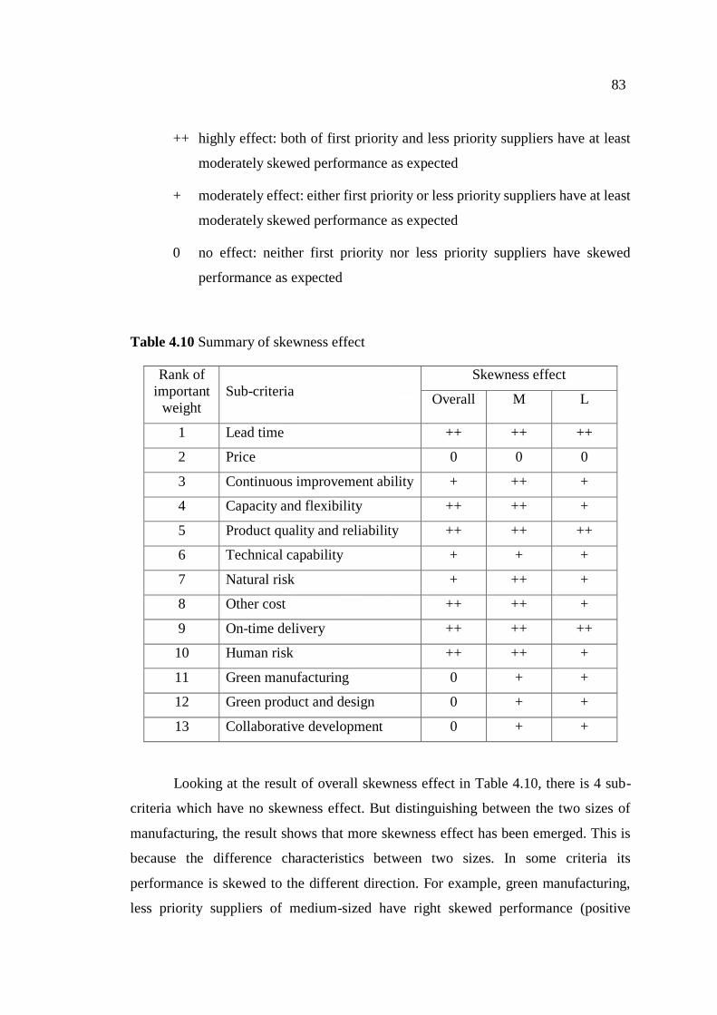
83
++ highly effect: both of first priority and less priority suppliers have at least
moderately skewed performance as expected
+ moderately effect: either first priority or less priority suppliers have at least
moderately skewed performance as expected
0 no effect: neither first priority nor less priority suppliers have skewed
performance as expected
Table 4.10 Summary of skewness effect
Rank of
important
weight
Sub-criteria
Skewness effect
Overall M L
1 Lead time ++ ++ ++
2 Price 0 0 0
3 Continuous improvement ability + ++ +
4 Capacity and flexibility ++ ++ +
5 Product quality and reliability ++ ++ ++
6 Technical capability + + +
7 Natural risk + ++ +
8 Other cost ++ ++ +
9 On-time delivery ++ ++ ++
10 Human risk ++ ++ +
11 Green manufacturing 0 + +
12 Green product and design 0 + +
13 Collaborative development 0 + +
Looking at the result of overall skewness effect in Table 4.10, there is 4 sub-
criteria which have no skewness effect. But distinguishing between the two sizes of
manufacturing, the result shows that more skewness effect has been emerged. This is
because the difference characteristics between two sizes. In some criteria its
performance is skewed to the different direction. For example, green manufacturing,
less priority suppliers of medium-sized have right skewed performance (positive

84
skewness), while first priority suppliers of large-sized manufacturers have left skewed
performance (negative skewness). Combining both sizes deducted their opposite effect
of skewness. Therefore, the overall result shows no effect of skewness at all. Hence, to
discuss on skewness effect, the classification between sizes of company is necessary.
However, the level of skewness effect is different between both sizes. Figure
4.8 and 4.9 present the comparison of skewness level on each size of manufacturer.
Skewness effect plays stronger role on medium-sized manufacturers than large-sized
manufacturers. As presented in Figure 4.8, more than half of sup-criteria of medium-
sized manufacturers have high skewness effect. Different from medium-sized, more
than half of sub-criteria of large-sized company have moderate skewness effect as
presented in Figure 4.9.
Figure 4.8 Ratio of skewness effect of medium-sized manufacturers
no effect, 8%
moderate,
31%
high, 62%

85
Figure 4.9 Ratio of skewness effect of large-sized manufacturers
Siz
e of
com
pan
y
L
Price (2)
Conti. imp. ability (4)
Capacity and flexibility (6)
Tech.capability (3)
Natural risk (10)
Other cost (5)
Human risk (9)
Green manu. (12)
Green prod. & design (11)
Collab. devel. (13)
Lead time (1)
On-time delivery (7)
Product qual, & reli. (8)
M
Price (1)
Tech.capability (11)
Green manu. (7)
Green prod. & design (13)
Collab. devel. (12)
Lead time (2)
Conti. imp. ability (4)
Capacity and flexibility (5)
Product qual, & reli. (3)
Natural risk (6)
Other cost (10)
On-time delivery (9)
Human risk (8)
No effect moderate high
Level of effect
Figure 4.10 Level of skewness effect
no effect, 8%
moderate
effect, 69%
high effect,
23%
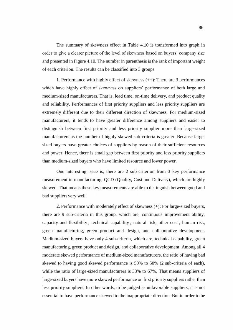
86
The summary of skewness effect in Table 4.10 is transformed into graph in
order to give a clearer picture of the level of skewness based on buyers’ company size
and presented in Figure 4.10. The number in parenthesis is the rank of important weight
of each criterion. The results can be classified into 3 groups.
1. Performance with highly effect of skewness (++): There are 3 performances
which have highly effect of skewness on suppliers’ performance of both large and
medium-sized manufacturers. That is, lead time, on-time delivery, and product quality
and reliability. Performances of first priority suppliers and less priority suppliers are
extremely different due to their different direction of skewness. For medium-sized
manufacturers, it tends to have greater difference among suppliers and easier to
distinguish between first priority and less priority supplier more than large-sized
manufacturers as the number of highly skewed sub-criteria is greater. Because large-
sized buyers have greater choices of suppliers by reason of their sufficient resources
and power. Hence, there is small gap between first priority and less priority suppliers
than medium-sized buyers who have limited resource and lower power.
One interesting issue is, there are 2 sub-criterion from 3 key performance
measurement in manufacturing, QCD (Quality, Cost and Delivery), which are highly
skewed. That means these key measurements are able to distinguish between good and
bad suppliers very well.
2. Performance with moderately effect of skewness (+): For large-sized buyers,
there are 9 sub-criteria in this group, which are, continuous improvement ability,
capacity and flexibility , technical capability , natural risk, other cost , human risk,
green manufacturing, green product and design, and collaborative development.
Medium-sized buyers have only 4 sub-criteria, which are, technical capability, green
manufacturing, green product and design, and collaborative development. Among all 4
moderate skewed performance of medium-sized manufacturers, the ratio of having bad
skewed to having good skewed performance is 50% to 50% (2 sub-criteria of each),
while the ratio of large-sized manufacturers is 33% to 67%. That means suppliers of
large-sized buyers have more skewed performance on first priority suppliers rather than
less priority suppliers. In other words, to be judged as unfavorable suppliers, it is not
essential to have performance skewed to the inappropriate direction. But in order to be
87
judged as first priority suppliers, besides consideration of average and variance of
performance, suppliers should have performance skewed to the expected direction.
Figure 4.11 presents the list of moderate skewed performances as well as their
size of company.
Siz
e of
com
pan
y
Good skewed Bad skewed
M
Technical capability
Collaborative development
Green manufacturing
Green product and design
L
Technical capability
Green manufacturing
Green product and design
Collaborative development
Continuous improvement ability
Capacity and flexibility
Figure 4.11 Moderate sub-criteria of each size of buyers and types of suppliers
It is no doubt that large-sized manufacturers have sufficient resources more
than medium-sized. So they have ability to rapidly adjust themselves to cope with
changing in terms of design, process or quantity. Also with their knowledge and
technology, they do not rely much on suppliers. Therefore, first priority supplier in the
perspective of large-sized companies are not required to have tendency to improve their
performance in the criteria of continuous improvement ability, capacity and flexibility,
and collaborative development. But this is different from technical capability criteria.
First priority suppliers of both medium and large-sized manufacturers have skewed
performance, while less priority suppliers have no skewness. This reflects that
technology is important issue for electronics industry, especially in the age that
technology is developed so fast. Hence, even unfavorable suppliers need to maintain
88
their performances to meet buyers’ expectation. Otherwise they would not survived in
this industry.
Both of sub-criteria in green supplier, first priority suppliers of large-sized
companies have tendency to have higher performance than expectation since their
performances are skewed to the expected direction, while first priority suppliers of
medium-sized companies have no tendency since their performance have no skew.
Even green issue has become world issue, but for Thai manufacturers, the issue has just
become mattered for few years, many of them are not still concern much about green
criteria as their important weight are ranked in the bottom three. This leads to the
thought of unnecessary to pay attention to improve green efficiency, especially for
medium-sized buyers. However, large-sized companies seem to concern on
environmental issues more than medium-sized. Therefore, first prioity suppliers of
large-sized must have skewed performances as shown in the result. In contrast, less
priority suppliers of medium-sized companies have skewed performance while large-
sized companies’ suppliers have no skew.
One interesting issue is unfavorable suppliers’ performance of other cost criteria
for large-sized buyers are not skewed as we expected. Because of buyers’ power over
suppliers, buyers can forced suppliers to monitor their performances avoiding failing to
meet buyers’ expectation even unfavorable suppliers.
3. Performance with no effect of skewness (0): Most of criteria have fluctuated
performance with tendency to differ from average efficiency, only price has no
skewness effect on both of first priority and less priority suppliers of M and L-sized
companies. This is because of the actual price cannot be much varied as it depends on
acceptable price or the contract made by both of buyer and supplier. However, other
cost which is in the same main criteria of cost is significantly skewed as shown in the
result, so we cannot deny the effect of skewness on cost performance on buyer decision
at all.
In summary, it appears that, in perspective of performance tendency, first
priority suppliers (supplier who performs well and be the first priority to be selected)
and less priority suppliers (suppliers who has lowest historical performance and be the
last choice to be selected) are different. Upon the hypothesis of skewness effect, either
89
performance skewness of first priority or less priority suppliers can support the
existence of skewness effect.
As aforementioned, performance perspective in this research can be classified
into 3 perspectives:
1. Performance efficiency measured by mean
2. Performance stability measured by standard deviation
3. Performance tendency measured by skewness
Apparently, skewness plays important role on suppliers’ performance but to
compare skewness effect with other performance perspectives, statistical hypothesis
testing is applied in order to give guidance to suppliers of which perspective should be
improved. The paired sample t-Test is used to compare the difference of performance
evaluating between first priority and less priority suppliers for each criteria in each
perspective. The hypothesis are:
H0: performance efficiency of first priority and less priority suppliers are equal
H1: performance efficiency of first priority and less priority suppliers are
different
H0: performance stability of first priority and less priority suppliers are equal
H1: performance stability of first priority and less priority suppliers are different
H0: performance tendency of first priority and less priority suppliers are equal
H1: performance tendency of first priority and less priority suppliers are
different
With the significance level equal to 0.05, the results are shown in Table 4.11
ranked by importance weight. This table summarizes the effect of each performance
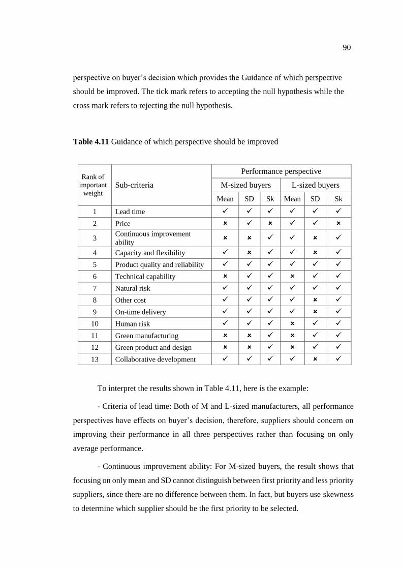
90
perspective on buyer’s decision which provides the Guidance of which perspective
should be improved. The tick mark refers to accepting the null hypothesis while the
cross mark refers to rejecting the null hypothesis.
Table 4.11 Guidance of which perspective should be improved
Rank of important
weight Sub-criteria
Performance perspective
M-sized buyers L-sized buyers
Mean SD Sk Mean SD Sk
1 Lead time
2 Price
3 Continuous improvement
ability
4 Capacity and flexibility
5 Product quality and reliability
6 Technical capability
7 Natural risk
8 Other cost
9 On-time delivery
10 Human risk
11 Green manufacturing
12 Green product and design
13 Collaborative development
To interpret the results shown in Table 4.11, here is the example:
- Criteria of lead time: Both of M and L-sized manufacturers, all performance
perspectives have effects on buyer’s decision, therefore, suppliers should concern on
improving their performance in all three perspectives rather than focusing on only
average performance.
- Continuous improvement ability: For M-sized buyers, the result shows that
focusing on only mean and SD cannot distinguish between first priority and less priority
suppliers, since there are no difference between them. In fact, but buyers use skewness
to determine which supplier should be the first priority to be selected.

91
For both of medium and large-sized manufacturers, skewness plays greater role
on performance than other perspectives. As presented in Figure 4.11 and 4.12, the
number of sub-criteria which can be used to distinguish between first priority and less
priority suppliers of skewness is greater than other perspectives. In other words, only
price cannot be discriminated by skewness. Therefore, Table 4.10 provides guidance of
which perspective should be improved and concerned.
Figure 4.12 Comparison of perspective effect of medium-sized manufactures
Figure 4.13 Comparison of perspective effect of large-sized manufactures
The interesting point obtaining is, for all criteria except price, only a perspective
that matters to buyer’s decision is skewness. So if suppliers would like to improve
62%69%
92%
0%
20%
40%
60%
80%
100%
mean SD skewness
Per
cent
level
of
effe
ct
69%62%
92%
0%
20%
40%
60%
80%
100%
mean SD skewness
Per
cent
level
of
effe
ct
92
themselves and become the first priority supplier, they should focus on their skewness
rather than mean or variance. This concludes that skewness should not be neglect when
making decision of supplier selecting and evaluating problem.
4.5 Developing Decision Matrix
The previous section proves that skewness between good and bad suppliers is
different and play important roles when evaluating suppliers. Therefore, when buyers
make a decision of which supplier should be selected, skewness should be included into
the decision model. In order to develop decision matrix considering skewness, the
concept of FMEA was modified. In FMEA, the risk level is measured by multiplying 3
combinations together, which are, severity, occurrence, and detectability. There is a
researcher applied this concept in order to select supplier (P-S. Chen and Wu, 2013). It
suggested to select supplier with lowest risk failure in order to avoid the possibility to
be failure or the possibility that supplier would perform worse than expected. But in
this research, it aims to measure the success ability, which means the possibility that
supplier would perform better than expected. In this section, first the developing matrix
is discussed, follows by validating matrix.
4.5.1 Developing Matrix by adpting FMEA
To select supplier by using FMEA method proposed by P.-S. Chen and Wu
(2013), the objective is to select supplier who has lowest risk of failure. In contrary to
select supplier based on risk perspective, this research aim to develop supplier selection
method based on the potential success or the tendency of supplier to perform better than
buyer’s expectation. Therefore, the new approach to select suppliers called Success
Mode Skewness Analysis (SMSA) is proposed. This approach is based on MVS
concept which the assumption is supplier with greatest expected performance does not
necessary be the best supplier but average performance, variance of performance and
skewness should combine together in order to evaluate among suppliers.
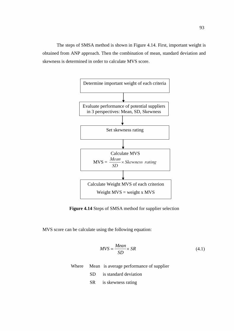
93
The steps of SMSA method is shown in Figure 4.14. First, important weight is
obtained from ANP approach. Then the combination of mean, standard deviation and
skewness is determined in order to calculate MVS score.
Figure 4.14 Steps of SMSA method for supplier selection
MVS score can be calculate using the following equation:
SRSD
MeanMVS (4.1)
Where Mean is average performance of supplier
SD is standard deviation
SR is skewness rating
Evaluate performance of potential suppliers
in 3 perspectives: Mean, SD, Skewness
Set skewness rating
Determine important weight of each criteria
Calculate MVS
MVS =
Calculate Weight MVS of each criterion
Weight MVS = weight x MVS

94
From equation 4.1, MVS is calculated by multiplying the reciprocal of CV and
skewness rating. Good supplier should have low CV and skewed performance to the
expected direction. The ratio of mean to SD in the equation represents the reciprocal of
CV which means the higher of this reciprocal, the better supplier. Hence, it can be
interpreted that good suppliers should have high MVS score. But for skewness, the
skewness value are not directly input to the equation but transformed into skewness
rating based on Bulmer’s rule of skewness but slightly adjusted the interpretation of
skewness value. Figure 4.15 presents the comparison between Bulmer’s rule and
adjusted skewness rating for positive skewed performance.
Figure 4.15 Comparison between Bulmer’s rule of skewness and skewness rating
Because performance can skewed to either expected direction or the opposite,
skeweness rating have both of positive and negative value depends on its direction. If
performance is skewed to the expected direction, then skewness rating are positive
value, otherwise skewness rating is negative value. Supposed that there is a supplier
who has performance skewed to the disfavor direction, the MVS of this supplier would
be negative value, since CV is positive. Therefore, total weight MVS of this supplier
will be deducted by this negative weight MVS. By using this algorithm, it is able to
0
1
0.5
Skewness value Bulmer’s rule Skewness rating
0.75
No skew
High
No skew
No to moderate Moderate
Moderate to high
High

95
include skewness effect into the decision matrix. The skewness rating is presented in
Table 4.12.
Table 4.12 Skewness rating
Skewness Rating Description
Expected Opposite
No skew 1 -1 5.05.0 Sk
No skew to moderate skew 2 -2 5.075.0 Sk or
75.05.0 Sk
Moderate to high skew 3 -3 75.01 Sk or
175.0 Sk
Highly skew 4 -4 1Sk or 1Sk
In summary, selecting supplier using FMEA is the approach emphasizes on
risk’s perspective while SMSA takes tendency to perform better into account. With
different perspective, the objective of the two methods are certainly different. FMEA
seeks for suppliers who has lower risk of failure, while SMSA seeks for suppliers who
has tendency to improve their performance. The differences between the two methods
is summarized and presented in Figure 4.16.
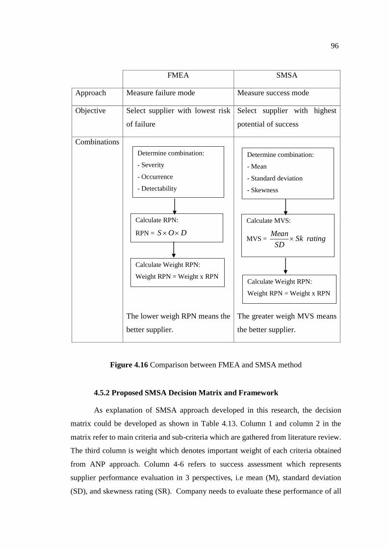
96
FMEA SMSA
Approach Measure failure mode Measure success mode
Objective Select supplier with lowest risk
of failure
Select supplier with highest
potential of success
Combinations
The lower weigh RPN means the
better supplier.
The greater weigh MVS means
the better supplier.
Figure 4.16 Comparison between FMEA and SMSA method
4.5.2 Proposed SMSA Decision Matrix and Framework
As explanation of SMSA approach developed in this research, the decision
matrix could be developed as shown in Table 4.13. Column 1 and column 2 in the
matrix refer to main criteria and sub-criteria which are gathered from literature review.
The third column is weight which denotes important weight of each criteria obtained
from ANP approach. Column 4-6 refers to success assessment which represents
supplier performance evaluation in 3 perspectives, i.e mean (M), standard deviation
(SD), and skewness rating (SR). Company needs to evaluate these performance of all
Determine combination:
- Severity
- Occurrence
- Detectability
Calculate RPN:
RPN = DOS
Calculate Weight RPN:
Weight RPN = Weight x RPN
Determine combination:
- Mean
- Standard deviation
- Skewness
Calculate MVS:
MVS = ratingSkSD
Mean
Calculate Weight RPN:
Weight RPN = Weight x RPN
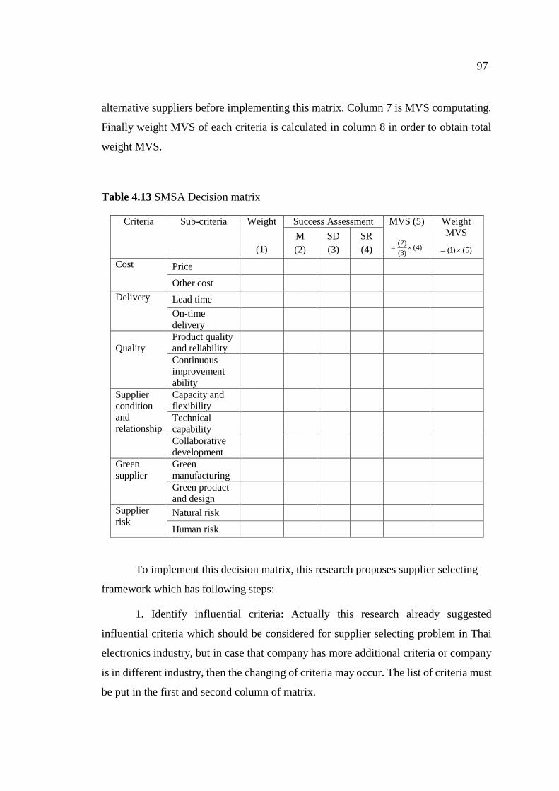
97
alternative suppliers before implementing this matrix. Column 7 is MVS computating.
Finally weight MVS of each criteria is calculated in column 8 in order to obtain total
weight MVS.
Table 4.13 SMSA Decision matrix
Criteria Sub-criteria Weight
(1)
Success Assessment MVS (5)
)4()3(
)2(
Weight MVS
)5()1(
M
(2)
SD
(3)
SR
(4)
Cost
Price
Other cost
Delivery
Lead time
On-time
delivery
Quality
Product quality and reliability
Continuous improvement
ability
Supplier condition and
relationship
Capacity and flexibility
Technical capability
Collaborative development
Green
supplier
Green
manufacturing
Green product and design
Supplier risk
Natural risk
Human risk
To implement this decision matrix, this research proposes supplier selecting
framework which has following steps:
1. Identify influential criteria: Actually this research already suggested
influential criteria which should be considered for supplier selecting problem in Thai
electronics industry, but in case that company has more additional criteria or company
is in different industry, then the changing of criteria may occur. The list of criteria must
be put in the first and second column of matrix.

98
2. Identify important weight: Compare importance of each criteria then put the
important weight in the third column. Actually there are many methods to use in order
to obtain important weight but this research suggests ANP approach as this method
consider the dependency among criteria and able to deal with both of qualitative and
quantitative criteria.
3. Evaluate supplier performance: Evaluate historical performance of all
alternative suppliers into 3 characteristics, which are, mean (M), standard deviating
(SD), and skewness. Then put the data of M and SD in column 4 and column 5,
respectively.
4. Identify skewness rating: Set level of skewness rating then transform
skewness value into skewness rating (SR) and put the value of skewness rating in
column 6. If performance is skewed to the expected direction, then SR is positive.
Otherwise, SR is negative. Here are the suggested skewness rating
5.05.0 Sk SR = 1 or SR = -1
5.075.0 Sk or 75.05.0 Sk SR = 2 or SR = -2
75.01 Sk or 175.0 Sk SR = 3 or SR = -3
1Sk or 1Sk SR = 4 or SR = -4
5. Compute MVS: Calculate MVS by using the following equation then put
MVS in column 7.
ratingSkSD
Mean
6. Calculate weight MVS: Calculate weight MVS which is the multiplication
between weight (column 3) and MVS (column 7).
7. Select supplier: Supplier who has highest total weight MVS is supplier who
has highest possibility to perform better than expected.
Table 4.14 shows the example of implementing decision matrix.

99
Tab
le 4
.14 E
xam
ple
of
imple
men
ting d
ecis
ion m
atri
x
S
uppli
er B
Wei
ght
MV
S
1.4
7
-0.7
7
-1.7
5
1.1
6
2.6
7
5.1
8
0.1
3
-6.7
2
0.8
2
-1.6
1.2
8
-2.8
9
-1.3
2
-2.3
4
MV
S
12.7
5
-8.7
3
-24
21.6
27.2
7
60
2.4
-93.6
9.5
5
-18.4
6
30
-39.6
-18
Tota
l
Succ
ess
Ass
essm
ent
SR
1
-2
-4
1
1
1
1
-4
1
-3
1
-2
-3
SD
0.6
67
1.8
3
7.5
4.1
7
1.8
3
1.1
67
1.6
7
3.3
33
7.3
3
6.5
2.5
4.1
7
6.6
67
M
8.5
8
45
90
50
70
4
78
70
40
75
82
40
Suppli
er A
Wei
ght
MV
S
2.3
1
1.8
5
1.3
1
3.4
3
3.5
2
2.4
2
1.0
1
-6.8
9
2.1
3
2.3
4
1.0
3
2.3
4
2.3
8
19.1
2
MV
S
20
20.5
7
18
64
36
28
19.2
-96
24.7
5
27
24
32
32.3
1
Tota
l
Succ
ess
Ass
essm
ent
SR
1
4
4
4
4
4
4
4
3
1
1
3
4
SD
0.8
1.1
67
2.5
3
1.6
67
5
0.8
33
3.3
33
4
6.6
67
3.3
33
5
0.8
M
8
6
45
96
60
70
4
80
99
60
80
80
70
Wei
ght
0.1
153
0.0
877
0.0
729
0.0
536
0.0
978
0.0
864
0.0
526
0.0
718
0.0
86
0.0
866
0.0
428
0.0
731
0.0
735
Sub
-cri
teri
a
Pri
ce
Oth
er c
ost
Lea
d t
ime
On-t
ime
del
iver
y
Gre
en
man
ufa
cturi
ng
Gre
en p
rodu
ct a
nd
des
ign
Pro
duct
qual
ity a
nd
reli
abil
ity
Conti
nuous
impro
vem
ent
abil
ity
Nat
ura
l ri
sk
Hum
an r
isk
Cap
acit
y a
nd
flex
ibil
ity
Tec
hnic
al c
apab
ilit
y
Coll
abora
tive
dev
elopm
ent
Mai
n c
rite
ria
Cost
Del
iver
y
Gre
en s
uppli
er
Qual
ity
Suppli
er r
isk
Suppli
er’s
condit
ion a
nd
rela
tionsh
ip

100
From the decision matrix in Table 4.14, supplier A and B are evaluated. The
result shows that total weight MVS of supplier A and B are 19.12 and -2.35,
respectively. This indicates that, supplier A has higher possibility to be success or
perform better than buyer’s expected. In contrast, B has possibility to perform worse
than A and also worse than buyer’s expected as its weight MVS is negative. Therefore,
in this case, the decision matrix suggests buyer to select supplier A rather than B.
4.5.2 Decision Matrix Validation
The verification of the proposed decision matrix is conducted by comparing the
result between excluding and including skewness in the decision matrix. In
questionnaire, the respondent is asking to evaluate performance of 2 suppliers. One is
the most prefer supplier who is the first priority to be selected, and another one is less
priority supplier. Performance of these two types of supplier as well as important weight
of each company is used as the input data. The result of which supplier should be
selected from each decision matrix is compared with the judgment of buyer’s obtained
from questionnaire. If the judgments are the same, then it is count as match result. The
steps of verification is illustrated in Figure 4.17
Compare the matching between result of matrix and buyer’s judgment, the
assumption is the judgment of purchasing manager who has great experience in
purchasing and dealing with suppliers is the right decision. Because it reflect the real
decision of selecting supplier. Therefore, supplier who has the best performance must
is the one who is selected.

101
Figure 4.17 Validation of decision matrix
In Figure 4.17, using decision matrix which ignoring skewness, the
overall %match is 75%, on the other hand there is 25% of mismatch result. Classified
by size, the %match of medium-sized and large-sized manufacturing is about 78% and
71%, respectively. Large-sized manufacturers have larger gap of mismatch. Using the
decision matrix which include skewness into consideration, all sample companies have
the same judgment as buyer’s selection.
Important weight from ANP approach
Excluding skewness:
Including skewness:
Compare the result with
the buyer’s judgment
Compare the result with
the buyer’s judgment
Compare the “match” count
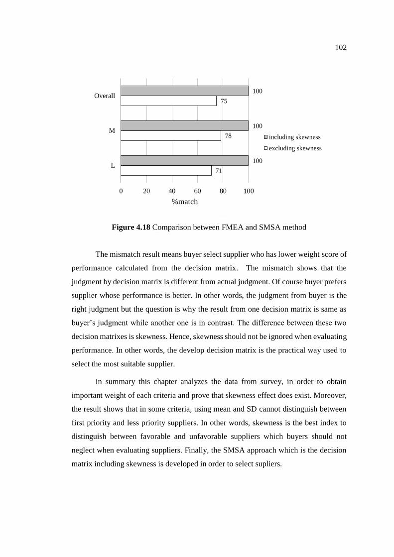
102
Figure 4.18 Comparison between FMEA and SMSA method
The mismatch result means buyer select supplier who has lower weight score of
performance calculated from the decision matrix. The mismatch shows that the
judgment by decision matrix is different from actual judgment. Of course buyer prefers
supplier whose performance is better. In other words, the judgment from buyer is the
right judgment but the question is why the result from one decision matrix is same as
buyer’s judgment while another one is in contrast. The difference between these two
decision matrixes is skewness. Hence, skewness should not be ignored when evaluating
performance. In other words, the develop decision matrix is the practical way used to
select the most suitable supplier.
In summary this chapter analyzes the data from survey, in order to obtain
important weight of each criteria and prove that skewness effect does exist. Moreover,
the result shows that in some criteria, using mean and SD cannot distinguish between
first priority and less priority suppliers. In other words, skewness is the best index to
distinguish between favorable and unfavorable suppliers which buyers should not
neglect when evaluating suppliers. Finally, the SMSA approach which is the decision
matrix including skewness is developed in order to select supliers.
71
78
75
100
100
100
0 20 40 60 80 100
L
M
Overall
%match
including skewness
excluding skewness
103
CHAPTER 5
CONCLUSION
This chapter concludes this research as well as its implication and
recommendation for future study.
5.1 Conclusion and Discussion
. Among several activities in logistics management, this research concentrating
on supplier selection problem which is one of important decision to be made in
purchasing and procurement activity. This research has 2 objectives. One is to identify
influential criteria and their important weight of supplier selection problem for Thai
electronics industry. Another objective is to develop decision matrices for selecting
supplier based on mean-variance-skewness.
To conduct this research, the initial set of criteria are gathered from literature
review and confirmed by experts in purchasing. Totally, there are 6 main criteria with
13 sub-criteria. With many criteria involved in making a decision to select the most
appropriate supplier, this research identified important weight of each criteria by using
ANP approach. Also this research introduced the important role of skewness. In
supplier selection problem, normally buying firms choose supplier which has best
performance. But supplier with greatest expected performance or highest average
performance does not mean the most suitable one. That is to say that, actually
performance should be measured into 3 perspectives, mean, variance and skewness (M-
V-S) combined together.
From literature review, it is found that the maximum sample size from previous
study in similar topic is 60 respondents. Therefore, this research set minimum sample
size required equals to 60 sample sizes. The data was collected by 2 ways, face-to-face
interview and questionnaire. The result from both ways are not significantly different.
However, it is found that collecting data by using questionnaire required more time,
especially the part of comparison among criteria. Because when it was found that
inconsistency existed, the questionnaire was sent back to respondent to re-judge.

104
Totally 77 sample sizes were collected. 53 samples are from interview whereas 24
samples are from questionnaire.
From result conclusion in Table 5.1, lead time is the highest influential factor
on supplier selection, follows by price, continuous improvement ability, capacity and
flexibility and product quality, and reliability, respectively. The results indicate the
nature of nowadays business environment which is more time sensitive and higher
responsive.
Table 5.1 Result conclusions
Rank
Weigh Sub-criteria
Effect of Performance perspective
M-sized buyers L-sized buyers
Mean SD Sk Mean SD Sk
1 0.0910 Lead time
2 0.0869 Price
3 0.0806 Continuous improvement ability
4 0.0791 Capacity and flexibility
5 0.0786 Product quality and reliability
6 0.0766 Technical capability
7 0.0755 Natural risk
8 0.0751 Other cost
9 0.0750 On-time delivery
10 0.0736 Human risk
11 0.0711 Green manufacturing
12 0.0690 Green product and design
13 0.0678 Collaborative development
In order to develop decision matrix, the existence of skewness effect is proved
prior to developing decision matrix. The data of performance evaluation between first
priority supplier and less priority was collected and analyzed. Performance are
measured in 3 characteristics, which are, mean, SD, and skewness as shown in Table
5.1. The result surprisingly shows that, in some criteria, there is no difference on mean
and SD between first priority and less priority suppliers. Only skewness does. For

105
example, green manufacturing, and green product and design. Also, skewness is the
best index to distinguish between first priority and less priority suppliers, while mean
is the worst index. This result indicates that when evaluating supplier, consideration
only on mean and SD is not enough, but skewness should also be considered.
The result analysis proved that skewness of performance between first priority
and less priority suppliers are skewed to different direction. While performance of good
suppliers are skewed to the expected direction, for example, lead time is right-skewed,
performance of bad suppliers are skewed to opposite direction. This indicates that good
suppliers should have tendency to perform better than buyers’ expectation. In contrast,
bad suppliers perform worse than expectation or promised performance.
Figure 5.1 Relationship between important weight ranking and skewness effect
From Figure 5.1, the vertical axis is the ranking of important weight based on
important weight in descending order. It shows that skewness effect has no relationship
between rankings. Criteria with high or low important weight are all having skewness
1
2
3
4
5
6
7
8
9
10
11
12
13
Ran
kin
g o
f im
po
rtan
t w
eight
no effect moderate high no effect moderate high
Medium-sized Large-sized

106
effect. Some have moderated effect while some have highly effect. But there is no
significant relationship between ranking and skewness effect. However, skewness plays
more important role on suppliers’ performance of medium-sized manufacturers than
large-sized manufacturers.
Finally, this research develop decision matrix to for selecting proper supplier.
By adapting concept of FMEA (Failure Mode and Effects Analysis) which measure risk
or failure mode by determining severity, occurrence and detection of failure then
transform to RPN score. Greater RPN denotes higher chance of failure or lower
satisfaction. But instead of evaluate failure mode, this research evaluate supplier
performance based on success mode which is called Success Mode with Skewness
Analysis (SMSA) by considering performance efficiency, performance stability, and
performance tendency which is measured by mean, standard deviation, and skewness
respectively. Table 5.2 presents decision matrix proposed by this research.
Table 5.2 Decision matrix of SMSA approach
Criteria Sub-criteria Weight
(1)
Success Assessment MVS (5)
)4()3(
)2(
Weight MVS
)5()1(
M
(2)
SD
(3)
SR
(4)
Cost
Price
Other cost
Delivery
Lead time
On-time delivery
Quality
Product quality and
reliability
Continuous
improvement ability
Supplier condition
and relationship
Capacity and
flexibility
Technical capability
Collaborative
development
Green
supplier
Green
manufacturing
Green product and
design
Supplier
risk Natural risk
Human risk
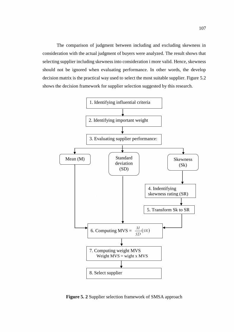
107
The comparison of judgment between including and excluding skewness in
consideration with the actual judgment of buyers were analyzed. The result shows that
selecting supplier including skewness into consideration i more valid. Hence, skewness
should not be ignored when evaluating performance. In other words, the develop
decision matrix is the practical way used to select the most suitable supplier. Figure 5.2
shows the decision framework for supplier selection suggested by this research.
Figure 5. 2 Supplier selection framework of SMSA approach
1. Identifying influential criteria
2. Identifying important weight
3. Evaluating supplier performance:
Mean (M) Standard
deviation
(SD)
Skewness
(Sk)
4. Indentifying skewness rating (SR)
5. Transform Sk to SR
6. Computing MVS =
7. Computing weight MVS Weight MVS = wight x MVS
8. Select supplier

108
Compare to previous literature in supplier selection problem, the criteria set
used in this research is similar to previous study. Since it is first extracted from
Disckson’s research in 1966 then selected most widely used criteria from review. But
since this research focuses on uncertainty or criteria which could have performance
fluctuated all the time, therefore only dynamic criteria are considered in this research.
In other words, to clearly explore skewness effect, this research disregards static criteria.
It is interesting for future research to combine both of static and dynamic criteria
together.
Also, when evaluating supplier performance, previous literatures always
considered on suppliers which have high expected average performance and low
variance but neglect uncertainty or the possibility that suppliers would performance
different from expected performance. Although there is a research studied by P-S. Chen
and Wu in 2013, which suggested to consider this uncertainty when evaluating supplier
performance. In the research by P-S. Chen and Wu, they defined the uncertainty by
emphasizing on the possibility of supplier to perform worse than expected or the
possibility to be failure by applying FMEA concept. But this research is focusing on
different aspect since it emphasizes on the possibility of supplier to perform better than
expected or the possibility to be success.
Moreover, this research not only suggest to combine all 3 performance
characteristics together when evaluating supplier performance, but it also compare the
effect of each characteristic or the ability to distinguish between first priority and less
priority suppliers. The surprising result is that skewness is the best index to distinguish
between first priority and less priority suppliers, while mean is the worst index
5.2 Implication
Findings and implications from this study has two-folds. The following parts
are discussed about implications from this research in term academic contributions and
business managerial implications.

109
5.2.1 Academic contribution
The most important academic contribution from this research is the discovering
and determining important role of skewness in supplier selection problem. In
circumstance which is full of uncertainties, supplier’s performance is unstable and
fluctuated throughout the period of time. In order to evaluating, nor only supplier
selection problem but also other decision problems in logistics field, researchers always
consider about mean and SD but ignoring skewness. From the result, it is found that
skewness really plays important role on supplier performance and it is the better index
which able to distinguish between favorable and unfavorable supplier than considering
only mean and SD as shown in Table 5.1. Hence, when evaluate performance, the
decision maker should consider performance skewness on top of the average and
variance (or standard deviation). This study is the empirical study of performance
evaluating of Thai electronics industry where 3 performance perspectives, average
efficiency, performance stability and performance tendency, are included in this study
Another contribution is the development of SMSA decision matrix which
consists of three performance perspectives measure by mean, standard deviation, and
skewness, and combines them together to propose new method to evaluate performance.
But instead of evaluating alternatives based on its failure mode like FMEA concept,
this research adapted to evaluate suppliers’ performance based on their success mode.
5.2.2 Business managerial Implication
The managerial implication in this research has 2 major practical implication.
One is for buyer firms, and another one is for supplier firms.
- For buyers, it is obvious that skewness has strongly impact on suppliers’
performances for both of good and bad suppliers. Therefore, to evaluate and compare
among potential suppliers, not only average performance or variance should be brought
into consideration, but buyers should also consider skewness by analyzing historical
performance of potential suppliers. To combine these 3 characteristics, the concept of
M-V-S evaluating can be implemented. This research proposed the decision matrix to

110
compare supplier performance. Therefore, buyers’ firm can implement the proposed
decision matrix in order to select supplier.
- For supplier’s side, this research provide the guidance of which performance
perspective should be improved for each criteria in order to become buyer’s first
priority supplier to be selected. From the conclusion shown in Table 5.1, judging by
buyer’s point of view, it shows that there is no difference between first priority and less
priority supplier in the perspective of mean and SD in some criteria. For example,
criteria of lead time of medium-sized manufactures, all 3 perspectives have difference
between first priority and less priority suppliers. Therefore, if less priority suppliers,
want to improve themselves to become first priority supplier, they should improve their
performance for all 3 characteristics. But for criteria of continuous improvement ability,
only skewness is different between less priority and first priority suppliers. This implies
that, if less priority suppliers want to improve themselves to become first priority
supplier, they should focus on improving their skewness or the ability to provide better
performance than buyers’ expectation rather than improving average performance or
performance stability. Because skewness is only one index which can be used to
distinguish between first priority and less priority suppliers.
5.3 Limitations
1. Data variation: This research studied about supplier selection problem of
Thai electronics industry which set home electrical machine as target group. However,
due to the vast number of manufacturers in this cluster as well as several manufacturer
types existed, there is still variation within sample size. Although this research tried to
minimize the variation by grouping samples based on their company size, there are
other source of variation, for example, types of manufacturer. But in practically,
companies do not produce exactly same product as their declaration based on TSIC
(Thailand Standard Industrial Classification) number of Department of Industrial
Works, Ministry of industry. Some companies produce not only product they registered
on TSIC type but other products as well. These products are mixed between similar
products to their product line or entirely different products. While some companies have
completely changed their product line from their TSIC types but did not change their
TSIC number. Also, some large-sized company which have many manufacturing plants,

111
each plant produces different product but they only registered their key product in TSIC.
Therefore, in this study only size of company are analyzed. The future research should
cover with this limitation.
2. Data collecting: In this research data collecting is conducted by 2 ways, i.e.,
interview and questionnaire. Although there is no different between the data obtained
from both ways but it is found that collecting data by using questionnaire is likely to
have more mistake and take longer time to correct. Especially in questionnaire section
1 which asking respondent to compare criteria based. In AHP approach, after getting
the comparisons, the results will be check if there is any inconsistency. For interviewing,
the inconsistency ratio can be calculated along with interviewing. . So if there is any
inconsistency, respondent will be asked to re-judgment the comparison instantly. But
using questionnaire, if the result is found that inconsistency existed in the comparison,
questionnaire will be sent back to respondent to re-judge. Then the result will be
analyzed again.
3. Bias in evaluating performance: Another issue is, there could be bias when
respondent evaluate performance of suppliers in some criteria. Especially if the time
period that supplier and buyer have been doing business together. With longer time,
buyers would have seen the changing or improvement on suppliers continuously.
Therefore, it has a chance that buyer will give higher satisfaction score to this supplier.
In the opposite, if supplier and buyer has been started doing business together for short
period, then it has a chance that buyer will give lower score to this supplier because the
improvement has not obviously occurred.
5.4 Future Research
One interesting issue that future research should consider is classification of
suppliers. In this research classifies customer into 2 types, 1) first priority supplier who
is the first option for buyer to buy product from, and 2) less priority supplier who has
least favorable and would be the last option for buyer to buy product from. The result
shows that, for less priority suppliers, number of criteria with no skewness effects of
large-sized manufacturers is greater than medium-sized manufacturers. This indicates
that, for buyers with large size, they have power over their suppliers. Therefore, they
112
can force their suppliers to maintain their performance. Even suppliers cannot improve
themselves or have better performance than buyers’ expectation, but they must keep
their level of efficiency not to be lower than customers’ expectation. This implies that,
actually suppliers have 3 types, 1) first priority suppliers who have performance skewed
to the expected direction or tend to perform better than expected, 2) moderate priority
suppliers who have no skewness effect or who perform exactly as expected, and 3) less
priority suppliers who have performance skewed to the opposite direction or perform
worse than expected. Future research should also consider suppliers who have
performance in between of first priority and less priority suppliers.
Moreover, comparison between 2 suppliers essentially judged by skewness may
not be able to apply in any case. Supposed that there are 2 alternative suppliers. One
provides very short lead time at 10 days but high instability and inappropriate skewness.
Another one provides longer lead time at 45 days with very low SD, high stability and
appropriate skewness. Of course buyers prefer suppliers who would perform better than
their expectation with high stability because it is easier for buyers to make plan and
operate. But since these 2 suppliers have much different average performance, it might
be worth to select supplier who perform worse than expected. Because even this
supplier would provide longer lead time than promised lead time but it is still very
shorter than the one who perform better than expected. Therefore, there might be the
cut-off point (critical point) that separate 2 decisions. Future research should take this
issue into consideration.
From findings in this study, skewness is an index that could be used to represent
the tendency of improvement. With high skewness, suppliers seem to have higher
performance than buyers’ expectation and tend to be able to improve their performance.
In addition, by improving on skewness, sooner or later, skewed performance seems to
gradually shift to the expected direction and be able to transform to normal distribution.
Future researchers should also study if improving skewness seems to be continuously
improved firm’s performance like PDCA concept.
113
REFERENCES
Aissaoui, N., Haouari, M., & Hassini, E. (2007). Supplier selection and order lot
sizing modeling: A review. Computers & Operations Research, 34, 3516-
3540.
Aksoy, A., & Öztürk, N. (2011). Supplier selection and performance evaluation in
just-in-time production environments. Expert Systems with Applications,
38(5), 6351-6359. doi:https://doi.org/10.1016/j.eswa.2010.11.104
Albino, V., & Garavelli, A. C. (1998). A neural network application to subcontractor
rating in construction firms. International Journal of Project Management,
16(1), 9-14. doi:https://doi.org/10.1016/S0263-7863(97)00007-0
Almannai, B., Greenough, R., & Kay, J. (2008). A decision support tool based on
QFD and FMEA for the selection of manufacturing automation technologies.
Robotics and Computer Integrated Manufacturing, 24(4), 501-507.
Bevilacqua, M., & Petroni, A. (2002). From Traditional Purchasing to Supplier
Management: A Fuzzy Logic-based Approach to Supplier Selection.
International Journal of Logistics Research and Applications, 5(3), 235-255.
doi:10.1080/1367556021000026691
Bhattacharya, A., Geraghty, J., & Young, P. (2010). Supplier selection paradigm: An
integrated hierarchical QFD methodology under multiple-criteria environment.
Applied Soft Computing, 10(4), 1013-1027.
doi:https://doi.org/10.1016/j.asoc.2010.05.025
Bruno, G., Esposito, E., Genovese, A., & Passaro, R. (2012). AHP-based approaches
for supplier evaluation: Problems and perspectives. Journal of Purchasing and
Supply Management, 18(3), 159-172.
doi:https://doi.org/10.1016/j.pursup.2012.05.001
Bulmer, M. G. (1979). Principles of Statistics. New York: Dover.
Cakravastia, A., Toha, I. S., & Nakamura, N. (2002). A two-stage model for the
design of supply chain networks. International Journal of Production

114
Economics, 80(3), 231-248. doi:https://doi.org/10.1016/S0925-
5273(02)00260-8
Castellano, R., & Cerqueti, R. (2014). Mean–Variance portfolio selection in presence
of infrequently traded stocks. European Journal of Operational Research,
234(2), 442-449. doi:https://doi.org/10.1016/j.ejor.2013.04.024
Cengiz, A. E., Aytekin, O., Ozdemir, I., Kusan, H., & Cabuk, A. (2017). A Multi-
criteria Decision Model for Construction Material Supplier Selection.
Procedia Engineering, 196(Supplement C), 294-301.
doi:https://doi.org/10.1016/j.proeng.2017.07.202
Chen, L.-H., & Ko, W.-C. (2009). Fuzzy linear programming models for new product
design using QFD with FMEA. Applied Mathematical Modelling, 33(2), 633-
647. doi:https://doi.org/10.1016/j.apm.2007.11.029
Chen, P.-S., & Wu, M.-T. (2013). A modified failure mode and effects analysis
method for supplier selection problems in the supply chain risk environment:
A case study. Computers & Industrial Engineering, 66(4), 634-642.
doi:https://doi.org/10.1016/j.cie.2013.09.018
Chen, Y. H., & Chao, R. J. (2012). Supplier selection using consistent fuzzy
preference relations. Expert Systems with Applications, 39(3), 3233-3240.
doi:https://doi.org/10.1016/j.eswa.2011.09.010
Chiou, C. Y., Hsu, C. W., & Hwang, W. Y. (2008, 8-11 Dec. 2008). Comparative
investigation on green supplier selection of the American, Japanese and
Taiwanese Electronics Industry in China. Paper presented at the 2008 IEEE
International Conference on Industrial Engineering and Engineering
Management.
Chiu, M. C., & Wong, H. Y. (2011). Mean–variance portfolio selection of
cointegrated assets. Journal of Economic Dynamics and Control, 35(8), 1369-
1385. doi:https://doi.org/10.1016/j.jedc.2011.04.003
Choy, K. L., Lee, W. B., & Lo, V. (2002). An intelligent supplier management tool
for benchmarking suppliers in outsource manufacturing. Expert Systems with
115
Applications, 22(3), 213-224. doi:https://doi.org/10.1016/S0957-
4174(01)00055-0
Dağsuyu, C., Göçmen, E., Narlı, M., & Kokangül, A. (2016). Classical and fuzzy
FMEA risk analysis in a sterilization unit. Computers & Industrial
Engineering, 101, 286-294. doi:https://doi.org/10.1016/j.cie.2016.09.015
Dargi, A., Anjomshoae, A., Galankashi, M. R., Memari, A., & Tap, M. B. M. (2014).
Supplier Selection: A Fuzzy-ANP Approach. Procedia Computer Science,
31(Supplement C), 691-700. doi:https://doi.org/10.1016/j.procs.2014.05.317
De Boer, L., Labro, E., & Morlacchi, P. (2001). A review of methods supporting
supplier selection. European Journal of Purchasing & Supply Management,
7(2), 75-89. doi:https://doi.org/10.1016/S0969-7012(00)00028-9
De Boer, L., Van Der Wegen, L., & Telgen, J. (1998). Outranking methods in support
of supplier selection. European Journal of Purchasing & Supply Management,
4(2), 109-118. doi:https://doi.org/10.1016/S0969-7012(97)00034-8
Dickson, G. W. (1966). Analysis of vendor selection systems and decisions. Journal
of Purchasing and Supply Management, 2(1), 5-17.
Dobos, I., & Vörösmarty, G. (2014). Green supplier selection and evaluation using
DEA-type composite indicators. International Journal of Production
Economics, 157(Supplement C), 273-278.
doi:https://doi.org/10.1016/j.ijpe.2014.09.026
Ekmekçioğlu, M., & Kutlu, A. (2012). A Fuzzy Hybrid Approach for Fuzzy Process
FMEA: An Application to a Spindle Manufacturing Process (Vol. 5).
Ellram, L. M., & Carr, A. (1994). Strategic purchasing: A history and review of the
literature. International Journal of Purchasing and Materials Management,
30(2), 10-18.
Eshtehardian, E., Ghodousi, P., & Bejanpour, A. (2013). Using ANP and AHP for the
supplier selection in the construction and civil engineering companies; Case
study of Iranian company. KSCE Journal of Civil Engineering, 17(2), 262-
270. doi:10.1007/s12205-013-1141-z
116
Fletcher, J. (1994). The mean-variance efficiency of benchmark portfolios: UK
evidence. Journal of Banking & Finance, 18(4), 673-685.
doi:https://doi.org/10.1016/0378-4266(94)00014-X
Gencer, C., & Gürpinar, D. (2007). Analytic network process in supplier selection: A
case study in an electronic firm. Applied Mathematical Modelling, 31(11),
2475-2486. doi:https://doi.org/10.1016/j.apm.2006.10.002
Ghodsypour, S. H., & O'Brien, C. (1998). A decision support system for supplier
selection using an integrated analytic hierarchy process and linear
programming. International Journal of Production Economics, 56-
57(Supplement C), 199-212. doi:https://doi.org/10.1016/S0925-
5273(97)00009-1
Ghodsypour, S. H., & O’Brien, C. (2001). The total cost of logistics in supplier
selection, under conditions of multiple sourcing, multiple criteria and capacity
constraint. International Journal of Production Economics, 73(1), 15-27.
doi:https://doi.org/10.1016/S0925-5273(01)00093-7
Gujarati, D. N. (2003). Basic Econometrics New York: McGraw-Hill.
Holt, G. D. (1998). Which contractor selection methodology? International Journal of
Project Management, 16(3), 153-164. doi:https://doi.org/10.1016/S0263-
7863(97)00035-5
Hozo, S. P., Djulbegovic, B., & Hozo, I. (2005). Estimating the mean and variance
from the median, range, and the size of a sample. BMC Medical Research
Methodology, 5(1), 13. doi:10.1186/1471-2288-5-13
Huang, X. (2012). Mean–variance models for portfolio selection subject to experts’
estimations. Expert Systems with Applications, 39(5), 5887-5893.
doi:https://doi.org/10.1016/j.eswa.2011.11.119
Humphreys, P., Huang, G., Cadden, T., & McIvor, R. (2007). Integrating design
metrics within the early supplier selection process. Journal of Purchasing and
Supply Management, 13(1), 42-52.
doi:https://doi.org/10.1016/j.pursup.2007.03.006
117
Jian, L., Fong‐Yuen, D., & Vinod, L. (2000). Using data envelopment analysis to
compare suppliers for supplier selection and performance improvement.
Supply Chain Management: An International Journal, 5(3), 143-150.
doi:doi:10.1108/13598540010338893
Joro, T., & Na, P. (2006). Portfolio performance evaluation in a mean–variance–
skewness framework. European Journal of Operational Research, 175(1),
446-461. doi:https://doi.org/10.1016/j.ejor.2005.05.006
Kannan, V. R., & Tan, K. C. (2002). Supplier Selection and Assessment: Their
Impact on Business Performance. Journal of Supply Chain Management,
38(3), 11-21. doi:10.1111/j.1745-493X.2002.tb00139.x
Katsikeas, C. S., Paparoidamis, N. G., & Katsikea, E. (2004). Supply source selection
criteria: The impact of supplier performance on distributor performance.
Industrial Marketing Management, 33(8), 755-764.
doi:https://doi.org/10.1016/j.indmarman.2004.01.002
Lee, A. H. I., Kang, H.-Y., Hsu, C.-F., & Hung, H.-C. (2009). A green supplier
selection model for high-tech industry. Expert Systems with Applications,
36(4), 7917-7927. doi:https://doi.org/10.1016/j.eswa.2008.11.052
Lemke, F., Goffin, K., Szwejczewski, M., Pfeiffer, R., & Lohmüller, B. (2000).
Supplier Base Management: Experiences from the UK and Germany.
International Journal of Logistics Management, 11(12), 45-58.
Li, X., & Zhao, C. (2009, 21-23 Oct. 2009). Selection of suppliers of vehicle
components based on green supply chain. Paper presented at the 2009 16th
International Conference on Industrial Engineering and Engineering
Management.
Liao, Z., & Rittscher, J. (2007). A multi-objective supplier selection model under
stochastic demand conditions. International Journal of Production Economics,
105(1), 150-159. doi:https://doi.org/10.1016/j.ijpe.2006.03.001

118
Liu, F.-H. F., & Hai, H. L. (2005). The voting analytic hierarchy process method for
selecting supplier. International Journal of Production Economics, 97(3), 308-
317. doi:https://doi.org/10.1016/j.ijpe.2004.09.005
Mafakheri, F., Breton, M., & Ghoniem, A. (2011). Supplier selection-order allocation:
A two-stage multiple criteria dynamic programming approach. International
Journal of Production Economics, 132(1), 52-57.
doi:https://doi.org/10.1016/j.ijpe.2011.03.005
Markowitz, H. (1952). PORTFOLIO SELECTION*. The Journal of Finance, 7(1),
77-91. doi:10.1111/j.1540-6261.1952.tb01525.x
Nelson, O. N., Muhamad, J., Loo, C. H., & Mat, S. A. (2005). Supplier selection and
management strategies and manufacturing flexibility. Journal of Enterprise
Information Management, 18(3), 330-349.
doi:doi:10.1108/17410390510592003
Saaty, T. L. (1980). The Analytic Hierarchy Process. New York: McGraw-Hill.
Saaty, T. L. (1999, August, 12-14 ). Fundamentals of the Analytic Network Process.
Paper presented at the ISAHP, Japan.
Saaty, T. L. (2008). Decision making with the analytic hierarchy process.
International Journal of Services Sciences, 1(1), 83-98.
Simić, D., Kovačević, I., Svirčević, V., & Simić, S. (2017). 50 years of fuzzy set
theory and models for supplier assessment and selection: A literature review.
Journal of Applied Logic, 24(Part A), 85-96.
doi:https://doi.org/10.1016/j.jal.2016.11.016
Timmerman, E. (1986). An Approach to Vendor Performance Evaluation. Journal of
Purchasing and Materials Management, 22(4), 2-8. doi:10.1111/j.1745-
493X.1986.tb00168.x
Toloo, M., & Nalchigar, S. (2011). A new DEA method for supplier selection in
presence of both cardinal and ordinal data. Expert Systems with Applications,
38(12), 14726-14731. doi:https://doi.org/10.1016/j.eswa.2011.05.008
119
Verma, R., & Pullman, M. E. (1998). An analysis of the supplier selection process.
Omega, 26(6), 739-750. doi:https://doi.org/10.1016/S0305-0483(98)00023-1
Weber, C. A. (1996). A data envelopment analysis approach to measuring vendor
performance. Supply Chain Management: An International Journal, 1(1), 28-
39. doi:doi:10.1108/13598549610155242
Weber, C. A., & Current, J. R. (1993). A multiobjective approach to vendor selection.
European Journal of Operational Research, 68(2), 173-184.
doi:https://doi.org/10.1016/0377-2217(93)90301-3
Weber, C. A., Current, J. R., & Benton, W. C. (1991). Vendor selection criteria and
methods. European Journal of Operational Research, 50(1), 2-18.
doi:https://doi.org/10.1016/0377-2217(91)90033-R
Weber, C. A., & Desai, A. (1996). Determination of paths to vendor market efficiency
using parallel coordinates representation: A negotiation tool for buyers.
European Journal of Operational Research, 90(1), 142-155.
doi:https://doi.org/10.1016/0377-2217(94)00336-X
Wu, D. (2009). Supplier selection: A hybrid model using DEA, decision tree and
neural network. Expert Systems with Applications, 36(5), 9105-9112.
doi:https://doi.org/10.1016/j.eswa.2008.12.039
Xiao, Z., Chen, W., & Li, L. (2012). An integrated FCM and fuzzy soft set for
supplier selection problem based on risk evaluation. Applied Mathematical
Modelling, 36(4), 1444-1454. doi:https://doi.org/10.1016/j.apm.2011.09.038
Yahya, S., & Kingsman, B. (1999). Vendor Rating for an Entrepreneur Development
Programme: A Case Study Using the Analytic Hierarchy Process Method. The
Journal of the Operational Research Society, 50(9), 916-930.
doi:10.2307/3010189
Yan, G. (2009, 15-17 May 2009). Research on Green Suppliers' Evaluation Based on
AHP & Genetic Algorithm. Paper presented at the 2009 International
Conference on Signal Processing Systems.

120
APPENDIX

121
APPENDEX A
แบบสอบถามเพอการวจย ดวยขาพเจา นางสาวอรณชา อนชตชาญชย นสตปรญญาเอก สาขาวชาการจดการดานโลจสตกส จฬาลงกรณมหาวทยาลย ก าลงด าเนนการวจยเรอง การคดเลอกผสงมอบแบบหลายเกณฑเชอมโยงโดยการประเมนความไมแนนอนของประสทธภาพ (Multi-dependent Criteria Supplier Selection with Uncertain
Performance Evaluation) โดยมวตถประสงคของงานวจยคอ 1. เพอศกษาถงปจจยทมผลในการคดเลอกผสงมอบ (Supplier) วตถดบในการผลตส าหรบอตสาหกรรมไฟฟาและอเลกทรอนกสในประเทศไทย 2. เพอพฒนาวธการในการตดสนเลอกผสงมอบทมประสทธภาพและแมนย ามากขน โดยพจารณาถงความไมแนนอนของประสทธภาพของผสงมอบ
เพอใหบรรลวตถประสงคงานวจยดงกลาวขางตน ผวจยตองก าหนดปจจยทมผลในการคดเลอกผสงมอบส าหรบอตสาหกรรมไฟฟาและอเลกทรอนกสในประเทศไทย เพอน าไปสรางแบบสอบถามทใชในการศกษาถงน าหนกความส าคญของแตละปจจยและพฒนาวธการคดเลอกผสงมอบตอไป
ขอมลจากทานจะเปนประโยชนอยางยงส าหรบงานวจยน ดงนน ผวจยจงใครขอความอนเคราะหจากทานในการตอบแบบสอบถามน รวมถงอาจมการสมภาษณเพมเตมเพอใหงานวจยนประสบความส าเรจลลวง ทงน ขอมลตาง ๆ จะถกเกบเปนความลบ ไมมการเผยแพร และไมมการเปดเผยขอมลเปนรายบคคล ตามหลกจรยธรรมและจรรยาบรรณทางวชาการ ทางผวจยขอขอบพระคณทานและองคกรของทานเปนอยางสง ทไดสละเวลาในการตอบแบบสอบถามนหรอการใหสมภาษณใด ๆ เพมเตม
ขอแสดงความนบถอ
อรณชา อนชตชาญชย
สวนท 1 ขอมลเบองตนของผตอบแบบสอบถาม
วนทตอบแบบสอบถาม: ____________________________
ชอ: _________________ นามสกล: __________________________ ต าแหนง: ___________________
บรษท/หนวยงาน: ______________________________ ประสบการณท างาน: _______________________
เบอรตดตอ: _________________________________ อเมลล: __________________________________
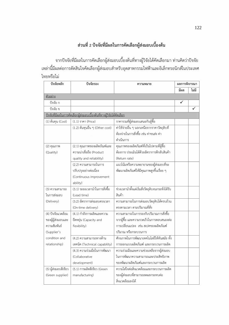
122
สวนท 2 ปจจยทมผลในการคดเลอกผสงมอบเบองตน
จากปจจยทมผลในการคดเลอกผสงมอบเบองตนททางผวจยไดคดเลอกมา ทานคดวาปจจยเหลานมผลตอการตดสนใจคดเลอกผสงมอบส าหรบอตสาหกรรมไฟฟาและอเลกทรอนกสในประเทศไทยหรอไม
ปจจยหลก ปจจยรอง ความหมาย ผลการพจารณา มผล ไมม
ตวอยาง ปจจย ก ปจจย ข
ปจจยทมผลในการคดเลอกผสงมอบเบองตนททางผวจยไดคดเลอก (1) ตนทน (Cost) (1.1) ราคา (Price) ราคารวมทผสงมอบเสนอกบผซอ (1.2) ตนทนอน ๆ (Other cost) คาใชจายอน ๆ นอกเหนอจากราคาวตถดบท
ตองจายในการสงซอ เชน คาขนสง คาด าเนนการ
(2) คณภาพ (Quality)
(2.1) คณภาพของผลตภณฑและความนาเชอถอ (Product quality and reliability)
คณภาพของผลตภณฑทเปนไปตามทผซอตองการ ประเมนไดดวยอตราการตกลบสนคา (Return rate)
(2.2) ความสามารถในการปรบปรงอยางตอเนอง (Continuous improvement ability)
แนวโนมหรอความพยายามของผสงมอบทจะพฒนาผลตภณฑใหมคณภาพสงขนเรอย ๆ
(3) ความสามารถในการสงมอบ (Delivery)
(3.1) ระยะเวลาน าในการสงซอ (Lead time)
ชวงเวลาน าตงแตเรมสงวตถดบจนกระทงไดรบสนคา
(3.2) อตราการสงมอบตรงเวลา (On-time delivery)
ความสามารถในการสงมอบวตถดบไดครบถวนตรงตามเวลา ตามปรมาณทสง
(4) ปจจยแวดลอมของผผสงมอบและความสมพนธ (Supplier’s condition and relationship)
(4.1) ก าลงการผลตและความยดหยน (Capacity and flexibility)
ความสามารถในการรองรบปรมาณการสงซอจากผซอ และความรวดเรวในการตอบสนองตอการเปลยนแปลง เชน สเปคของผลตภณฑ ปรมาณ หรอกระบวนการ
(4.2) ความสามารถทางดานเทคนค (Technical capability)
ศกยภาพในการพฒนาเทคโนโลยใหทนสมย ทงการออกแบบผลตภณฑ และกระบวนการผลต
(4.3) ความรวมมอในการพฒนา (Collaborative development)
ความรวมมอและความชวยเหลอจากผสงมอบในการพฒนาความสามารถและประสทธภาพของพฒนาผลตภณฑและกระบวนการผลต
(5) ผสงมอบสเขยว (Green supplier)
(5.1) การผลตสเขยว (Green manufacturing)
ความใสใจตอสงแวดลอมและกระบวนการผลตของผสงมอบทสามารถลดผลกระทบตอสงแวดลอมลงได

123
ปจจยหลก ปจจยรอง ความหมาย ผลการพจารณา มผล ไมม
(5.2) ผลตภณฑและการออกแบบสเขยว (Green product and design)
การออกแบบผลตภณฑและบรรจภณฑทค านงถงผลกระทบตอสงแวดลอม เชน เปนผลตภณฑทออกแบบน ากลบมาใชใหมได (Design for Recycle) หรอถอดประกอบไดงาย (Design for Disassembly)
(6) ความเสยง (Supplier risk)
(6.1) ความเสยงจากธรรมชาต (Natural risk)
โอกาสทประสทธภาพของผสงมอบจะไมเปนไปตามทคาด อนเนองมาจากภยธรรมชาต และปจจยภายนอกทควบคมไมได
(6.2) ความเสยงจากความผดพลาดของบคคล (Human risk)
โอกาสทประสทธภาพของผสงมอบจะไมเปนไปตามทคาดอนเนองมาจากความผดพลาดของพนกงานของผสงมอบ
สวนท 3 ปจจยเพมเตมและขอเสนอแนะอน ๆ
นอกเหนอจากปจจยทมผลในการคดเลอกผสงมอบเบองตนททางผวจยไดคดเลอกมาในสวนท 2 ทานคดวาปจจยตอไปนมผลตอการตดสนใจคดเลอกผสงมอบส าหรบอตสาหกรรมไฟฟาและอเลกทรอนกสในประเทศไทยหรอไม
ปจจย ความหมาย ผลการพจารณา มผล ไมม
ความสามารถในอดต (Performance history)
ความสามารถหรอผลงานในอดตของผสงมอบ
ทศนคต (Attitude)
ทศนคตของผสงมอบ หรอแนวคดในการท างานของผสงมอบ
ระบบการฝกอบรม (Training Aids)
ระบบการพฒนาบคคลากรของผสงมอบ รวมถงการชวยเหลอในการฝกอบรมพนกงานของผซอในกรณทจ าเปน
การควบคมการด าเนนงาน (Operating controls)
ความสามารถในการควบคมการปฏบตงานหรอกระบวนการ โดยเนนทผบรหารระดบลาง เชน มกระบวนการในการควบคมการปฏบตงานของพนกงาน มกระบวนการในการควบคมความสามารถของกระบวนการในการผลต (Process Capability) เปนตน
ความสามารถในการบรรจภณฑ (Packaging ability)
ความสามารถของผสงมอบในการพฒนาประสทธภาพของบรรจภณฑ
ความสามารถในการใหการบรการ (Repair service)
ความสามารถในการตอบสนองของผสงมอบในกรณทเกดปญหาตาง ๆ ขน
ความประทบใจ (Impression)
ความประทบใจทผซอมตอผสงมอบ
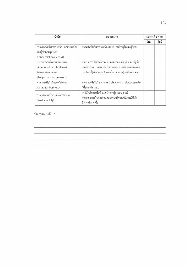
124
ปจจย ความหมาย ผลการพจารณา มผล ไมม
ความสมพนธระหวางพนกงานขององคกรของผซอและผสงมอบ (Labor relations record)
ความสมพนธระหวางพนกงานขององคกรผซอและผขาย
ปรมาณทเคยซอขายกนในอดต (Amount of past business)
ปรมาณการสงซอทผานมาในอดต หมายถง ผสงมอบทผซอเคยสงวตถดบในปรมาณมากกวามแนวโนมจะไดรบคดเลอก
ขอตกลงตางตอบแทน (Reciprocal arrangements)
แนวโนมทผสงมอบจะท าการซอสนคาจากผขายในอนาคต
ความกระตอรอรนของผสงมอบ (Desire for business)
ความกระตอรอรน ความเอาใจใส และความเตมใจชวยเหลอผซอจากผสงมอบ
ความสามารถในการใหการบรการ (Service ability)
การใหบรการหรอค าแนะน าจากผสงมอบ รวมถงความสามารถในการตอบสนองของผสงมอบในกรณทเกดปญหาตาง ๆ ขน
ขอเสนอแนะอน ๆ
____________________________________________________________________________________ ____________________________________________________________________________________ ____________________________________________________________________________________ ____________________________________________________________________________________ ____________________________________________________________________________________

125
APPENDIX B
แบบสอบถามเพอการวจย
ดวยขาพเจา นางสาวอรณชา อนชตชาญชย นสตปรญญาเอก สาขาวชาการจดการดานโลจสตกส จฬาลงกรณมหาวทยาลย ก าลงด าเนนการวจยเรอง การคดเลอกผสงมอบแบบหลายเกณฑเชอมโยงโดยการประเมนความไมแนนอนของประสทธภาพ (Multi-dependent Criteria Supplier Selection with Uncertain Performance Evaluation) โดยมวตถประสงคของงานวจยคอ
1. เพอศกษาถงปจจยทมผลในการคดเลอกผสงมอบ (Supplier) วตถดบในการผลตส าหรบอตสาหกรรมไฟฟาและอเลกทรอนกสในประเทศไทย
2. เพอพฒนาวธการในการตดสนเลอกผสงมอบทมประสทธภาพและแมนย ามากขน โดยพจารณาถงความไมแนนอนของประสทธภาพของผสงมอบ
เพอใหบรรลวตถประสงคงานวจยดงกลาวขางตน ทางผวจยตองการทราบน าหนกความส าคญของปจจยทงหลาย โดยแบบสอบถามชดนประกอบไปดวย 3 สวน ไดแก
- สวนท 1 การสอบถามขอมลเบองตนของผตอบแบบสอบถาม - สวนท 2 การเปรยบเทยบน าหนกความส าคญของแตละปจจย โดยประยกตใชเทคนคกระบวนการ
โครงขายเชงวเคราะห (Analytic Network Process) ซงตองใชการเปรยบเทยบแบบค โดยรายละเอยดและขนตอนการตอบแบบสอบถามจะไดน าเสนอถดไป
- สวนท 3 การประเมนประสทธภาพของผสงมอบในดานตาง ๆ โดยค านงถงความไมแนนอนของประสทธภาพ โดยผประเมนจะเลอกผสงมอบในปจจบน หรอผทเขาขายไดรบเลอกเปนผสงมอบทขายวตถดบเหมอนกน 2 ราย และท าการประเมนประสทธภาพของผสงมอบ
ขอมลจากทานจะเปนประโยชนอยางยงส าหรบงานวจยน ดงนน ผวจยจงใครขอความอนเคราะหจากทานในการตอบแบบสอบถาม รวมถงอาจมการสมภาษณเพมเตมเพอใหงานวจยนประสบความส าเรจลลวง ทงน ขอมลตาง ๆ จะถกเกบเปนความลบไมมการเผยแพร และไมมการเปดเผยขอมลเปนรายบคคล ตามหลกจรยธรรมและจรรยาบรรณทางวชาการ ทางผวจยขอขอบพระคณทานและองคกรของทานเปนอยางสง ทไดสละเวลาในการตอบแบบสอบถามนหรอการใหสมภาษณใด ๆ เพมเตม ขอแสดงความนบถอ อรณชา อนชตชาญชย

126
ตารางท 1 ปจจยหลก/ปจจยรองทมผลตอการตดสนใจคดเลอกผสงมอบ และความหมาย ปจจยหลก ปจจยรอง ความหมาย
(1) ตนทน (Cost) (1.1) ราคา (Price) ราคาจรงของวตถดบทผสงมอบเสนอกบผซอ (1.2) ตนทนอน ๆ (Other cost) คาใชจายอน ๆ นอกเหนอจากราคาวตถดบทตองจายใน
การสงซอ เชน คาขนสง คาด าเนนการ เปนตน (2) คณภาพ (Quality)
(2.1) คณภาพของผลตภณฑและความนาเชอถอ (Product quality and reliability)
คณภาพของผลตภณฑทเปนไปตามทผซอตองการ ประเมนไดดวยอตราการตกลบสนคา (Return rate)
(2.2) ความสามารถในการปรบปรงอยางตอเนอง (Continuous improvement ability)
แนวโนมหรอความพยายามของผสงมอบทจะพฒนาผลตภณฑใหมคณภาพสงขนเรอย ๆ
(3) ความสามารถในการสงมอบ (Delivery)
(3.1) ระยะเวลาน าในการสงซอ (Lead time)
ชวงเวลาน าตงแตเรมส งวตถดบจนกระทงไดรบสนคา
(3.2) อตราการสงมอบตรงเวลา (On-time delivery)
ความสามารถในการสงมอบวตถดบไดครบถวนตรงตามเวลา ตามปรมาณทส ง
(4) ปจจยแวดลอมของผสงมอบและความสมพนธ (Supplier’s condition and relationship)
(4.1) ก าลงการผลตและความยดหยน (Capacity and flexibility)
ความสามารถในการรองรบปรมาณการสงซอจากผซอ และความรวดเรวในการตอบสนองตอการเปลยนแปลง เชน สเปคของผลตภณฑ ปรมาณ หรอกระบวนการ
(4.2) ความสามารถทางดานเทคนค (Technical capability)
ศกยภาพในการพฒนาเทคโนโลยใหทนสมย ทงการออกแบบผลตภณฑ และกระบวนการผลต
(4.3) ความรวมมอในการพฒนา (Collaborative development)
ความรวมมอและความชวยเหลอจากผสงมอบในการพฒนาความสามารถและประสทธภาพของพฒนาผลตภณฑและกระบวนการผลต
(5) ผสงมอบสเขยว (Green supplier)
(5.1) การผลตสเขยว (Green manufacturing)
ความใสใจตอสงแวดลอมและกระบวนการผลตของผสงมอบทสามารถลดผลกระทบตอสงแวดลอมลงได
(5.2) ผลตภณฑและการออกแบบสเขยว (Green product and design)
การออกแบบผลตภณฑและบรรจภณฑทค านงถงผลกระทบตอสงแวดลอม เชน เปนผลตภณฑทออกแบบน ากลบมาใชใหมได (Design for Recycle) หรอถอดประกอบไดงาย (Design for Disassembly)
(6) ความเสยง (Supplier risk)
(6.1) ความเสยงจากธรรมชาต (Natural risk)
โอกาสทประสทธภาพของผสงมอบจะไมเปนไปตามทคาด อนเนองมาจากภยธรรมชาต และปจจยภายนอกทควบคมไมได
(6.2) ความเสยงจากความผดพลาดของบคคล (Human risk)
โอกาสทประสทธภาพของผสงมอบจะไมเปนไปตามทคาดอนเนองมาจากความผดพลาดของพนกงานของผสงมอบ

127
สวนท 1 ขอมลเบองตนของผตอบแบบสอบถาม
วนทตอบแบบสอบถาม: ชอ: นามสกล: ประสบการณท างาน: เบอรตดตอ: อเมลล: . ต าแหนง: บรษท/หนวยงาน: .
ประเภทบรษท บรษทคนไทย บรษทรวมทนกบตางชาต โปรดระบประเทศทรวมทน บรษทตางชาต ประเทศ (โปรดระบ)
ทนจดทะเบยน ไมเกน 50 ลานบาท 51-200 ลานบาท 200 ลานบาทขนไป
จ านวนพนกงาน ไมเกน 50 คน 51-200 คน 200 คนขนไป
วตถดบหลก (ทเปนชนสวน/อปกรณไฟฟาและอเลกทรอนกส) (โปรดระบ)
ผลตภณฑหลก (ทเปนชนสวน/อปกรณไฟฟาและอเลกทรอนกส) (โปรดระบ)
การสงซอวตถดบสวนใหญสงซอจากภายใน หรอน าเขาจากตางประเทศ (โปรดระบสดสวน) - สงซอจากภายในประเทศ % - น าเขาจากตางประเทศ %
ผลตภณฑสวนใหญขายภายในประเทศหรอสงออกไปยงตางประเทศ (โปรดระบสดสวน) - ขายภายในประเทศ % - สงออกไปตางประเทศ % (โปรดระบประเทศ)
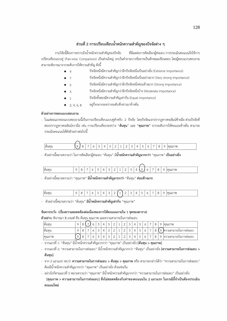
128
สวนท 2 การเปรยบเทยบนาหนกความสาคญของปจจยตาง ๆ
งานวจยนตองการทราบถงน าหนกความส าคญของปจจย ทมผลตอการคดเลอกผสงมอบ การประเมนคะแนนจงใชการเปรยบเทยบแบบค (Pair-wise Comparison) เปนสวนใหญ ยกเวนค าถามบางขออาจเปนลกษณะเขยนตอบ โดยผตอบแบบสอบถามสามารถพจารณาจากระดบการใหความส าคญ ดงน
9 ปจจยหนงมความส าคญกวาอกปจจยหนงเปนอยางยง (Extreme Importance)
7 ปจจยหนงมความส าคญกวาอกปจจยหนงเปนอยางมาก (Very strong importance)
5 ปจจยหนงมความส าคญกวาอกปจจยหนงคอนขางมาก (Strong importance)
3 ปจจยหนงมความส าคญกวาอกปจจยหนงบาง (Moderate importance)
1 ปจจยทงสองมความส าคญเทากน (Equal importance)
2, 4, 6, 8 อยกงกลางระหวางระดบทกลาวมาขางตน
ตวอยางการตอบแบบสอบถาม - ในแตละแถวของแบบสอบถามนเปนการเปรยบเทยบแบบคส าหรบ 2 ปจจย โดยปจจยแรกปรากฏทางคอลมนซายมอ สวนปจจยท
สองปรากฏทางคอลมนขวามอ เชน การเปรยบเทยบระหวาง “ตนทน” และ “คณภาพ” จากระดบการใหคะแนนขางตน สามารถประเมนคะแนนไดดงตวอยางตอไปน
ตนทน 9 8 7 6 5 4 3 2 1 2 3 4 5 6 7 8 9 คณภาพ
- ตวอยางนหมายความวา ในการคดเลอกผสงมอบ “ตนทน” มนาหนกความสาคญมากกวา “คณภาพ” เปนอยางยง
ตนทน 9 8 7 6 5 4 3 2 1 2 3 4 5 6 7 8 9 คณภาพ
- ตวอยางนหมายความวา “คณภาพ” มนาหนกความสาคญมากกวา “ตนทน” คอนขางมาก
ตนทน 9 8 7 6 5 4 3 2 1 2 3 4 5 6 7 8 9 คณภาพ
- ตวอยางนหมายความวา “ตนทน” มนาหนกความสาคญเทากบ “คณภาพ”
ขอควรระวง (เรองความสอดคลองตอเนองของการใหคะแนนภายใน 1 ชดของตาราง) ตวอยาง: พจารณา 3 เกณฑ คอ ตนทน คณภาพ และความสามารถในการสงมอบ
ตนทน 9 8 7 6 5 4 3 2 1 2 3 4 5 6 7 8 9 คณภาพ ตนทน 9 8 7 6 5 4 3 2 1 2 3 4 5 6 7 8 9 ความสามารถในการสงมอบ
คณภาพ 9 8 7 6 5 4 3 2 1 2 3 4 5 6 7 8 9 ความสามารถในการสงมอบ
- จากแถวท 1: “ตนทน” มน าหนกความส าคญมากกวา “คณภาพ” เปนอยางยง [ตนทน > คณภาพ] - จากแถวท 2: “ความสามารถในการสงมอบ” มน าหนกความส าคญมากกวา “ตนทน” เปนอยางยง [ความสามารถในการสงมอบ >
ตนทน] - จาก 2 แถวแรก พบวา ความสามารถในการสงมอบ > ตนทน > คณภาพ หรอ สามารถกลาวไดวา “ความสามารถในการสงมอบ”
ตองมน าหนกความส าคญมากกวา “คณภาพ” เปนอยางยง ดวยเชนกน - อยางไรกตามแถวท 3 หมายความวา “คณภาพ” มน าหนกความส าคญมากกวา “ความสามารถในการสงมอบ” เปนอยางยง
[คณภาพ > ความสามารถในการสงมอบ] ซงไมสอดคลองกบคาของคะแนนใน 2 แถวแรก ในกรณนจาเปนตองประเมนคะแนนใหม
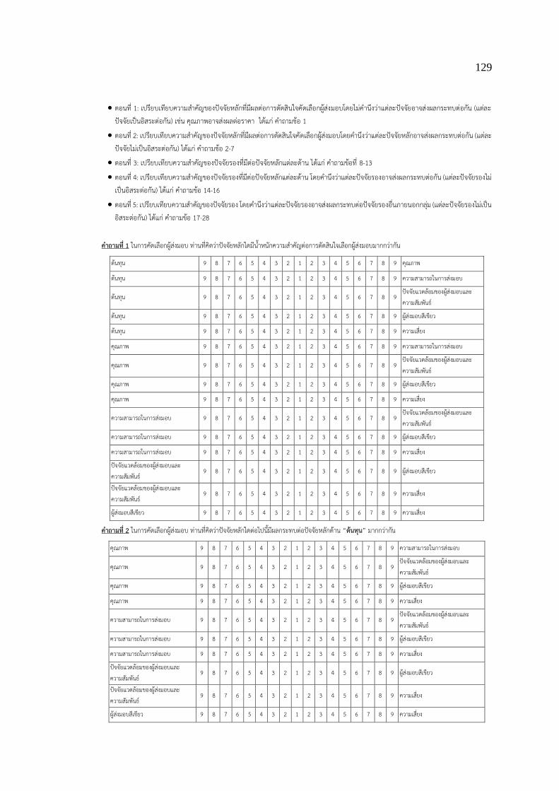
129
ตอนท 1: เปรยบเทยบความส าคญของปจจยหลกทมผลตอการตดสนใจคดเลอกผสงมอบโดยไมค านงวาแตละปจจยอาจสงผลกระทบตอกน (แตละปจจยเปนอสระตอกน) เชน คณภาพอาจสงผลตอราคา ไดแก ค าถามขอ 1
ตอนท 2: เปรยบเทยบความส าคญของปจจยหลกทมผลตอการตดสนใจคดเลอกผสงมอบโดยค านงวาแตละปจจยหลกอาจสงผลกระทบตอกน (แตละปจจยไมเปนอสระตอกน) ไดแก ค าถามขอ 2-7
ตอนท 3: เปรยบเทยบความส าคญของปจจยรองทมตอปจจยหลกแตละดาน ไดแก ค าถามขอท 8-13
ตอนท 4: เปรยบเทยบความส าคญของปจจยรองทมตอปจจยหลกแตละดาน โดยค านงวาแตละปจจยรองอาจสงผลกระทบตอกน (แตละปจจยรองไมเปนอสระตอกน) ไดแก ค าถามขอ 14-16
ตอนท 5: เปรยบเทยบความส าคญของปจจยรอง โดยค านงวาแตละปจจยรองอาจสงผลกระทบตอปจจยรองอนภายนอกกลม (แตละปจจยรองไมเปนอสระตอกน) ไดแก ค าถามขอ 17-28
คาถามท 1 ในการคดเลอกผสงมอบ ทานทคดวาปจจยหลกใดมน าหนกความส าคญตอการตดสนใจเลอกผสงมอบมากกวากน
ตนทน 9 8 7 6 5 4 3 2 1 2 3 4 5 6 7 8 9 คณภาพ
ตนทน 9 8 7 6 5 4 3 2 1 2 3 4 5 6 7 8 9 ความสามารถในการสงมอบ
ตนทน 9 8 7 6 5 4 3 2 1 2 3 4 5 6 7 8 9 ปจจยแวดลอมของผสงมอบและความสมพนธ
ตนทน 9 8 7 6 5 4 3 2 1 2 3 4 5 6 7 8 9 ผสงมอบสเขยว
ตนทน 9 8 7 6 5 4 3 2 1 2 3 4 5 6 7 8 9 ความเสยง
คณภาพ 9 8 7 6 5 4 3 2 1 2 3 4 5 6 7 8 9 ความสามารถในการสงมอบ
คณภาพ 9 8 7 6 5 4 3 2 1 2 3 4 5 6 7 8 9 ปจจยแวดลอมของผสงมอบและความสมพนธ
คณภาพ 9 8 7 6 5 4 3 2 1 2 3 4 5 6 7 8 9 ผสงมอบสเขยว
คณภาพ 9 8 7 6 5 4 3 2 1 2 3 4 5 6 7 8 9 ความเสยง
ความสามารถในการสงมอบ 9 8 7 6 5 4 3 2 1 2 3 4 5 6 7 8 9 ปจจยแวดลอมของผสงมอบและความสมพนธ
ความสามารถในการสงมอบ 9 8 7 6 5 4 3 2 1 2 3 4 5 6 7 8 9 ผสงมอบสเขยว
ความสามารถในการสงมอบ 9 8 7 6 5 4 3 2 1 2 3 4 5 6 7 8 9 ความเสยง
ปจจยแวดลอมของผสงมอบและความสมพนธ
9 8 7 6 5 4 3 2 1 2 3 4 5 6 7 8 9 ผสงมอบสเขยว
ปจจยแวดลอมของผสงมอบและความสมพนธ
9 8 7 6 5 4 3 2 1 2 3 4 5 6 7 8 9 ความเสยง
ผสงมอบสเขยว 9 8 7 6 5 4 3 2 1 2 3 4 5 6 7 8 9 ความเสยง
คาถามท 2 ในการคดเลอกผสงมอบ ทานทคดวาปจจยหลกใดตอไปนมผลกระทบตอปจจยหลกดาน “ตนทน” มากกวากน
คณภาพ 9 8 7 6 5 4 3 2 1 2 3 4 5 6 7 8 9 ความสามารถในการสงมอบ
คณภาพ 9 8 7 6 5 4 3 2 1 2 3 4 5 6 7 8 9 ปจจยแวดลอมของผสงมอบและความสมพนธ
คณภาพ 9 8 7 6 5 4 3 2 1 2 3 4 5 6 7 8 9 ผสงมอบสเขยว
คณภาพ 9 8 7 6 5 4 3 2 1 2 3 4 5 6 7 8 9 ความเสยง
ความสามารถในการสงมอบ 9 8 7 6 5 4 3 2 1 2 3 4 5 6 7 8 9 ปจจยแวดลอมของผสงมอบและความสมพนธ
ความสามารถในการสงมอบ 9 8 7 6 5 4 3 2 1 2 3 4 5 6 7 8 9 ผสงมอบสเขยว
ความสามารถในการสงมอบ 9 8 7 6 5 4 3 2 1 2 3 4 5 6 7 8 9 ความเสยง
ปจจยแวดลอมของผสงมอบและความสมพนธ
9 8 7 6 5 4 3 2 1 2 3 4 5 6 7 8 9 ผสงมอบสเขยว
ปจจยแวดลอมของผสงมอบและความสมพนธ
9 8 7 6 5 4 3 2 1 2 3 4 5 6 7 8 9 ความเสยง
ผสงมอบสเขยว 9 8 7 6 5 4 3 2 1 2 3 4 5 6 7 8 9 ความเสยง

130
คาถามท 3 ในการคดเลอกผสงมอบ ทานทคดวาปจจยหลกใดตอไปนมผลกระทบตอปจจยหลกดาน “คณภาพ” มากกวากน
ตนทน 9 8 7 6 5 4 3 2 1 2 3 4 5 6 7 8 9 ความสามารถในการสงมอบ
ตนทน 9 8 7 6 5 4 3 2 1 2 3 4 5 6 7 8 9 ปจจยแวดลอมของผสงมอบและความสมพนธ
ตนทน 9 8 7 6 5 4 3 2 1 2 3 4 5 6 7 8 9 ผสงมอบสเขยว
ตนทน 9 8 7 6 5 4 3 2 1 2 3 4 5 6 7 8 9 ความเสยง
ความสามารถในการสงมอบ 9 8 7 6 5 4 3 2 1 2 3 4 5 6 7 8 9 ปจจยแวดลอมของผสงมอบและความสมพนธ
ความสามารถในการสงมอบ 9 8 7 6 5 4 3 2 1 2 3 4 5 6 7 8 9 ผสงมอบสเขยว
ความสามารถในการสงมอบ 9 8 7 6 5 4 3 2 1 2 3 4 5 6 7 8 9 ความเสยง
ปจจยแวดลอมของผสงมอบและความสมพนธ
9 8 7 6 5 4 3 2 1 2 3 4 5 6 7 8 9 ผสงมอบสเขยว
ปจจยแวดลอมของผสงมอบและความสมพนธ
9 8 7 6 5 4 3 2 1 2 3 4 5 6 7 8 9 ความเสยง
ผสงมอบสเขยว 9 8 7 6 5 4 3 2 1 2 3 4 5 6 7 8 9 ความเสยง
คาถามท 4 ในการคดเลอกผสงมอบ ทานทคดวาปจจยหลกใดตอไปนมผลกระทบตอปจจยหลกดาน “ความสามารถในการสงมอบ” มากกวากน
ตนทน 9 8 7 6 5 4 3 2 1 2 3 4 5 6 7 8 9 คณภาพ
ตนทน 9 8 7 6 5 4 3 2 1 2 3 4 5 6 7 8 9 ปจจยแวดลอมของผสงมอบและความสมพนธ
ตนทน 9 8 7 6 5 4 3 2 1 2 3 4 5 6 7 8 9 ผสงมอบสเขยว
ตนทน 9 8 7 6 5 4 3 2 1 2 3 4 5 6 7 8 9 ความเสยง
คณภาพ 9 8 7 6 5 4 3 2 1 2 3 4 5 6 7 8 9 ปจจยแวดลอมของผสงมอบและความสมพนธ
คณภาพ 9 8 7 6 5 4 3 2 1 2 3 4 5 6 7 8 9 ผสงมอบสเขยว
คณภาพ 9 8 7 6 5 4 3 2 1 2 3 4 5 6 7 8 9 ความเสยง
ปจจยแวดลอมของผสงมอบและความสมพนธ
9 8 7 6 5 4 3 2 1 2 3 4 5 6 7 8 9 ผสงมอบสเขยว
ปจจยแวดลอมของผสงมอบและความสมพนธ
9 8 7 6 5 4 3 2 1 2 3 4 5 6 7 8 9 ความเสยง
ผสงมอบสเขยว 9 8 7 6 5 4 3 2 1 2 3 4 5 6 7 8 9 ความเสยง
คาถามท 5 ในการคดเลอกผสงมอบ ทานทคดวาปจจยหลกใดตอไปนมผลกระทบตอปจจยหลกดาน “ปจจยแวดลอมของผสงมอบและความสมพนธ” มากกวากน
ตนทน 9 8 7 6 5 4 3 2 1 2 3 4 5 6 7 8 9 คณภาพ
ตนทน 9 8 7 6 5 4 3 2 1 2 3 4 5 6 7 8 9 ความสามารถในการสงมอบ
ตนทน 9 8 7 6 5 4 3 2 1 2 3 4 5 6 7 8 9 ผสงมอบสเขยว
ตนทน 9 8 7 6 5 4 3 2 1 2 3 4 5 6 7 8 9 ความเสยง
คณภาพ 9 8 7 6 5 4 3 2 1 2 3 4 5 6 7 8 9 ความสามารถในการสงมอบ
คณภาพ 9 8 7 6 5 4 3 2 1 2 3 4 5 6 7 8 9 ผสงมอบสเขยว
คณภาพ 9 8 7 6 5 4 3 2 1 2 3 4 5 6 7 8 9 ความเสยง
ความสามารถในการสงมอบ 9 8 7 6 5 4 3 2 1 2 3 4 5 6 7 8 9 ผสงมอบสเขยว
ความสามารถในการสงมอบ 9 8 7 6 5 4 3 2 1 2 3 4 5 6 7 8 9 ความเสยง
ผสงมอบสเขยว 9 8 7 6 5 4 3 2 1 2 3 4 5 6 7 8 9 ความเสยง

131
คาถามท 6 ในการคดเลอกผสงมอบ ทานทคดวาปจจยหลกใดตอไปนมผลกระทบตอปจจยหลกดาน “ผสงมอบสเขยว” มากกวากน
ตนทน 9 8 7 6 5 4 3 2 1 2 3 4 5 6 7 8 9 คณภาพ
ตนทน 9 8 7 6 5 4 3 2 1 2 3 4 5 6 7 8 9 ความสามารถในการสงมอบ
ตนทน 9 8 7 6 5 4 3 2 1 2 3 4 5 6 7 8 9 ปจจยแวดลอมของผสงมอบและความสมพนธ
ตนทน 9 8 7 6 5 4 3 2 1 2 3 4 5 6 7 8 9 ความเสยง
คณภาพ 9 8 7 6 5 4 3 2 1 2 3 4 5 6 7 8 9 ความสามารถในการสงมอบ
คณภาพ 9 8 7 6 5 4 3 2 1 2 3 4 5 6 7 8 9 ปจจยแวดลอมของผสงมอบและความสมพนธ
คณภาพ 9 8 7 6 5 4 3 2 1 2 3 4 5 6 7 8 9 ความเสยง
ความสามารถในการสงมอบ 9 8 7 6 5 4 3 2 1 2 3 4 5 6 7 8 9 ปจจยแวดลอมของผสงมอบและความสมพนธ
ความสามารถในการสงมอบ 9 8 7 6 5 4 3 2 1 2 3 4 5 6 7 8 9 ความเสยง
ปจจยแวดลอมของผสงมอบและความสมพนธ
9 8 7 6 5 4 3 2 1 2 3 4 5 6 7 8 9 ความเสยง
คาถามท 7 ในการคดเลอกผสงมอบ ทานทคดวาปจจยหลกใดตอไปนมผลกระทบตอปจจยหลกดาน “ความเสยง” มากกวากน
ตนทน 9 8 7 6 5 4 3 2 1 2 3 4 5 6 7 8 9 คณภาพ
ตนทน 9 8 7 6 5 4 3 2 1 2 3 4 5 6 7 8 9 ความสามารถในการสงมอบ
ตนทน 9 8 7 6 5 4 3 2 1 2 3 4 5 6 7 8 9 ปจจยแวดลอมของผสงมอบและความสมพนธ
ตนทน 9 8 7 6 5 4 3 2 1 2 3 4 5 6 7 8 9 ผสงมอบสเขยว
คณภาพ 9 8 7 6 5 4 3 2 1 2 3 4 5 6 7 8 9 ความสามารถในการสงมอบ
คณภาพ 9 8 7 6 5 4 3 2 1 2 3 4 5 6 7 8 9 ปจจยแวดลอมของผสงมอบและความสมพนธ
คณภาพ 9 8 7 6 5 4 3 2 1 2 3 4 5 6 7 8 9 ผสงมอบสเขยว
ความสามารถในการสงมอบ 9 8 7 6 5 4 3 2 1 2 3 4 5 6 7 8 9 ปจจยแวดลอมของผสงมอบและความสมพนธ
ความสามารถในการสงมอบ 9 8 7 6 5 4 3 2 1 2 3 4 5 6 7 8 9 ผสงมอบสเขยว
ปจจยแวดลอมของผสงมอบและความสมพนธ
9 8 7 6 5 4 3 2 1 2 3 4 5 6 7 8 9 ผสงมอบสเขยว
คาถามท 8 ส าหรบปจจยหลกดาน “ตนทน” ทานทคดวาปจจยรองใดตอไปนมผลกระทบตอปจจยหลกดงกลาวมากกวากน
ราคา 9 8 7 6 5 4 3 2 1 2 3 4 5 6 7 8 9 ตนทนอน ๆ
คาถามท 9 ส าหรบปจจยหลกดาน “คณภาพ” ทานทคดวาปจจยรองใดตอไปนมผลกระทบตอปจจยหลกดงกลาวมากกวากน
คณภาพของผลตภณฑและความนาเชอถอ
9 8 7 6 5 4 3 2 1 2 3 4 5 6 7 8 9 ความสามารถในการปรบปรงอยางตอเนอง
คาถามท 10 ส าหรบปจจยหลกดาน “ความสามารถในการสงมอบ” ทานทคดวาปจจยรองใดตอไปนมผลกระทบตอปจจยหลกดงกลาวมากกวากน
ระยะเวลาน าในการสงซอ 9 8 7 6 5 4 3 2 1 2 3 4 5 6 7 8 9 อตราการสงมอบตรงเวลา
คาถามท 11 ส าหรบปจจยหลกดาน “ปจจยแวดลอมของผสงมอบและความสมพนธ” ทานทคดวาปจจยรองใดตอไปนมผลกระทบตอปจจยหลกดงกลาวมากกวากน
ก าลงการผลตและความยดหยน 9 8 7 6 5 4 3 2 1 2 3 4 5 6 7 8 9 ความสามารถทางดานเทคนค
ก าลงการผลตและความยดหยน 9 8 7 6 5 4 3 2 1 2 3 4 5 6 7 8 9 ความรวมมอในการพฒนา
ความสามารถทางดานเทคนค 9 8 7 6 5 4 3 2 1 2 3 4 5 6 7 8 9 ความรวมมอในการพฒนา

132
คาถามท 12 ส าหรบปจจยหลกดาน “ผสงมอบสเขยว” ทานทคดวาปจจยรองใดตอไปนมผลกระทบตอปจจยหลกดงกลาวมากกวากน
การผลตสเขยว 9 8 7 6 5 4 3 2 1 2 3 4 5 6 7 8 9 ผลตภณฑและการออกแบบสเขยว
คาถามท 13 ส าหรบปจจยหลกดาน “ความเสยง” ทานทคดวาปจจยรองใดตอไปนมผลกระทบตอปจจยหลกดงกลาวมากกวากน
ความเสยงจากธรรมชาต 9 8 7 6 5 4 3 2 1 2 3 4 5 6 7 8 9 ความเสยงจากความผดพลาดของบคคล
คาถามท 14 ทานทคดวาปจจยรองใดตอไปนมผลกระทบตอปจจยรองดาน “กาลงการผลตและความยดหยน” มากกวากน
ความสามารถทางดานเทคนค 9 8 7 6 5 4 3 2 1 2 3 4 5 6 7 8 9 ความรวมมอในการพฒนา
คาถามท 15 ทานทคดวาปจจยรองใดตอไปนมผลกระทบตอปจจยรองดาน “ความสามารถทางดานเทคนค” มากกวากน
ก าลงการผลตและความยดหยน 9 8 7 6 5 4 3 2 1 2 3 4 5 6 7 8 9 ความรวมมอในการพฒนา
คาถามท 16 ทานทคดวาปจจยรองใดตอไปนมผลกระทบตอปจจยรองดาน “ความรวมมอในการพฒนา” มากกวากน
ก าลงการผลตและความยดหยน 9 8 7 6 5 4 3 2 1 2 3 4 5 6 7 8 9 ความสามารถทางดานเทคนค
คาถามท 17 ทานทคดวาปจจยรองใดตอไปนมผลกระทบตอปจจยรองดาน “ราคา” มากกวากน
คณภาพของผลตภณฑและความนาเชอถอ
9 8 7 6 5 4 3 2 1 2 3 4 5 6 7 8 9 ความสามารถในการปรบปรงอยางตอเนอง
ระยะเวลาน าในการสงซอ 9 8 7 6 5 4 3 2 1 2 3 4 5 6 7 8 9 อตราการสงมอบตรงเวลา
ก าลงการผลตและความยดหยน 9 8 7 6 5 4 3 2 1 2 3 4 5 6 7 8 9 ความสามารถทางดานเทคนค
ก าลงการผลตและความยดหยน 9 8 7 6 5 4 3 2 1 2 3 4 5 6 7 8 9 ความรวมมอในการพฒนา
ความสามารถทางดานเทคนค 9 8 7 6 5 4 3 2 1 2 3 4 5 6 7 8 9 ความรวมมอในการพฒนา
การผลตสเขยว 9 8 7 6 5 4 3 2 1 2 3 4 5 6 7 8 9 ผลตภณฑและการออกแบบสเขยว
ความเสยงจากธรรมชาต 9 8 7 6 5 4 3 2 1 2 3 4 5 6 7 8 9 ความเสยงจากความผดพลาดของบคคล
คาถามท 18 ทานทคดวาปจจยรองใดตอไปนมผลกระทบตอปจจยรองดาน “ตนทนอน ๆ ” มากกวากน
คณภาพของผลตภณฑและความนาเชอถอ
9 8 7 6 5 4 3 2 1 2 3 4 5 6 7 8 9 ความสามารถในการปรบปรงอยางตอเนอง
ระยะเวลาน าในการสงซอ 9 8 7 6 5 4 3 2 1 2 3 4 5 6 7 8 9 อตราการสงมอบตรงเวลา
ก าลงการผลตและความยดหยน 9 8 7 6 5 4 3 2 1 2 3 4 5 6 7 8 9 ความสามารถทางดานเทคนค
ก าลงการผลตและความยดหยน 9 8 7 6 5 4 3 2 1 2 3 4 5 6 7 8 9 ความรวมมอในการพฒนา
ความสามารถทางดานเทคนค 9 8 7 6 5 4 3 2 1 2 3 4 5 6 7 8 9 ความรวมมอในการพฒนา
การผลตสเขยว 9 8 7 6 5 4 3 2 1 2 3 4 5 6 7 8 9 ผลตภณฑและการออกแบบสเขยว
ความเสยงจากธรรมชาต 9 8 7 6 5 4 3 2 1 2 3 4 5 6 7 8 9 ความเสยงจากความผดพลาดของบคคล
คาถามท 19 ทานทคดวาปจจยรองใดตอไปนมผลกระทบตอปจจยรองดาน “คณภาพของผลตภณฑและความนาเชอถอ” มากกวากน
ราคา 9 8 7 6 5 4 3 2 1 2 3 4 5 6 7 8 9 ตนทนอน ๆ
ระยะเวลาน าในการสงซอ 9 8 7 6 5 4 3 2 1 2 3 4 5 6 7 8 9 อตราการสงมอบตรงเวลา
ก าลงการผลตและความยดหยน 9 8 7 6 5 4 3 2 1 2 3 4 5 6 7 8 9 ความสามารถทางดานเทคนค
ก าลงการผลตและความยดหยน 9 8 7 6 5 4 3 2 1 2 3 4 5 6 7 8 9 ความรวมมอในการพฒนา
ความสามารถทางดานเทคนค 9 8 7 6 5 4 3 2 1 2 3 4 5 6 7 8 9 ความรวมมอในการพฒนา
การผลตสเขยว 9 8 7 6 5 4 3 2 1 2 3 4 5 6 7 8 9 ผลตภณฑและการออกแบบสเขยว
ความเสยงจากธรรมชาต 9 8 7 6 5 4 3 2 1 2 3 4 5 6 7 8 9 ความเสยงจากความผดพลาดของบคคล

133
คาถามท 20 ทานทคดวาปจจยรองใดตอไปนมผลกระทบตอปจจยรองดาน “ความสามารถในการปรบปรงอยางตอเนอง” มากกวากน
ราคา 9 8 7 6 5 4 3 2 1 2 3 4 5 6 7 8 9 ตนทนอน ๆ
ระยะเวลาน าในการสงซอ 9 8 7 6 5 4 3 2 1 2 3 4 5 6 7 8 9 อตราการสงมอบตรงเวลา
ก าลงการผลตและความยดหยน 9 8 7 6 5 4 3 2 1 2 3 4 5 6 7 8 9 ความสามารถทางดานเทคนค
ก าลงการผลตและความยดหยน 9 8 7 6 5 4 3 2 1 2 3 4 5 6 7 8 9 ความรวมมอในการพฒนา
ความสามารถทางดานเทคนค 9 8 7 6 5 4 3 2 1 2 3 4 5 6 7 8 9 ความรวมมอในการพฒนา
การผลตสเขยว 9 8 7 6 5 4 3 2 1 2 3 4 5 6 7 8 9 ผลตภณฑและการออกแบบสเขยว
ความเสยงจากธรรมชาต 9 8 7 6 5 4 3 2 1 2 3 4 5 6 7 8 9 ความเสยงจากความผดพลาดของบคคล
คาถามท 21 ทานทคดวาปจจยรองใดตอไปนมผลกระทบตอปจจยรองดาน “ระยะเวลานาในการสงซอ” มากกวากน
ราคา 9 8 7 6 5 4 3 2 1 2 3 4 5 6 7 8 9 ตนทนอน ๆ
คณภาพของผลตภณฑและความนาเชอถอ
9 8 7 6 5 4 3 2 1 2 3 4 5 6 7 8 9 ความสามารถในการปรบปรงอยางตอเนอง
ก าลงการผลตและความยดหยน 9 8 7 6 5 4 3 2 1 2 3 4 5 6 7 8 9 ความสามารถทางดานเทคนค
ก าลงการผลตและความยดหยน 9 8 7 6 5 4 3 2 1 2 3 4 5 6 7 8 9 ความรวมมอในการพฒนา
ความสามารถทางดานเทคนค 9 8 7 6 5 4 3 2 1 2 3 4 5 6 7 8 9 ความรวมมอในการพฒนา
การผลตสเขยว 9 8 7 6 5 4 3 2 1 2 3 4 5 6 7 8 9 ผลตภณฑและการออกแบบสเขยว
ความเสยงจากธรรมชาต 9 8 7 6 5 4 3 2 1 2 3 4 5 6 7 8 9 ความเสยงจากความผดพลาดของบคคล
คาถามท 22 ทานทคดวาปจจยรองใดตอไปนมผลกระทบตอปจจยรองดาน “อตราการสงมอบตรงเวลา” มากกวากน
ราคา 9 8 7 6 5 4 3 2 1 2 3 4 5 6 7 8 9 ตนทนอน ๆ
คณภาพของผลตภณฑและความนาเชอถอ
9 8 7 6 5 4 3 2 1 2 3 4 5 6 7 8 9 ความสามารถในการปรบปรงอยางตอเนอง
ก าลงการผลตและความยดหยน 9 8 7 6 5 4 3 2 1 2 3 4 5 6 7 8 9 ความสามารถทางดานเทคนค
ก าลงการผลตและความยดหยน 9 8 7 6 5 4 3 2 1 2 3 4 5 6 7 8 9 ความรวมมอในการพฒนา
ความสามารถทางดานเทคนค 9 8 7 6 5 4 3 2 1 2 3 4 5 6 7 8 9 ความรวมมอในการพฒนา
การผลตสเขยว 9 8 7 6 5 4 3 2 1 2 3 4 5 6 7 8 9 ผลตภณฑและการออกแบบสเขยว
ความเสยงจากธรรมชาต 9 8 7 6 5 4 3 2 1 2 3 4 5 6 7 8 9 ความเสยงจากความผดพลาดของบคคล
คาถามท 23 ทานทคดวาปจจยรองใดตอไปนมผลกระทบตอปจจยรองดาน “กาลงการผลตและความยดหยน” มากกวากน
ราคา 9 8 7 6 5 4 3 2 1 2 3 4 5 6 7 8 9 ตนทนอน ๆ
คณภาพของผลตภณฑและความนาเชอถอ
9 8 7 6 5 4 3 2 1 2 3 4 5 6 7 8 9 ความสามารถในการปรบปรงอยางตอเนอง
ระยะเวลาน าในการสงซอ 9 8 7 6 5 4 3 2 1 2 3 4 5 6 7 8 9 อตราการสงมอบตรงเวลา
การผลตสเขยว 9 8 7 6 5 4 3 2 1 2 3 4 5 6 7 8 9 ผลตภณฑและการออกแบบสเขยว
ความเสยงจากธรรมชาต 9 8 7 6 5 4 3 2 1 2 3 4 5 6 7 8 9 ความเสยงจากความผดพลาดของบคคล
คาถามท 24 ทานทคดวาปจจยรองใดตอไปนมผลกระทบตอปจจยรองดาน “ความสามารถทางดานเทคนค” มากกวากน
ราคา 9 8 7 6 5 4 3 2 1 2 3 4 5 6 7 8 9 ตนทนอน ๆ
คณภาพของผลตภณฑและความนาเชอถอ
9 8 7 6 5 4 3 2 1 2 3 4 5 6 7 8 9 ความสามารถในการปรบปรงอยางตอเนอง
ระยะเวลาน าในการสงซอ 9 8 7 6 5 4 3 2 1 2 3 4 5 6 7 8 9 อตราการสงมอบตรงเวลา
การผลตสเขยว 9 8 7 6 5 4 3 2 1 2 3 4 5 6 7 8 9 ผลตภณฑและการออกแบบสเขยว
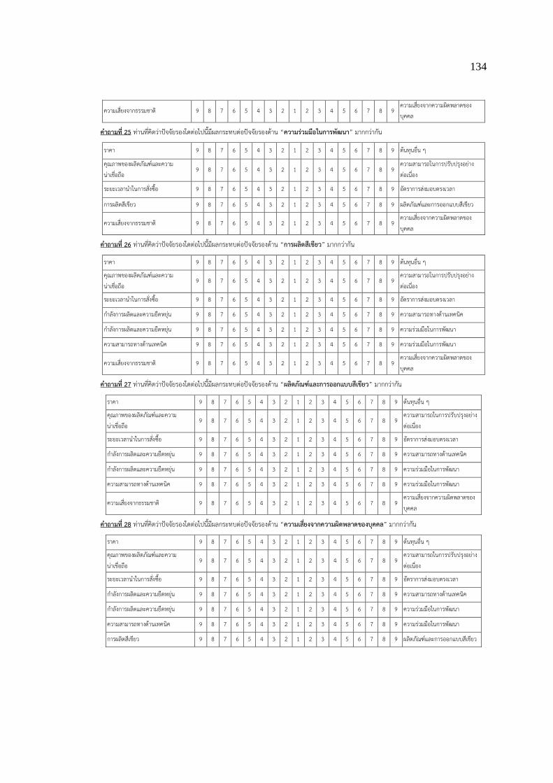
134
ความเสยงจากธรรมชาต 9 8 7 6 5 4 3 2 1 2 3 4 5 6 7 8 9 ความเสยงจากความผดพลาดของบคคล
คาถามท 25 ทานทคดวาปจจยรองใดตอไปนมผลกระทบตอปจจยรองดาน “ความรวมมอในการพฒนา” มากกวากน
ราคา 9 8 7 6 5 4 3 2 1 2 3 4 5 6 7 8 9 ตนทนอน ๆ
คณภาพของผลตภณฑและความนาเชอถอ
9 8 7 6 5 4 3 2 1 2 3 4 5 6 7 8 9 ความสามารถในการปรบปรงอยางตอเนอง
ระยะเวลาน าในการสงซอ 9 8 7 6 5 4 3 2 1 2 3 4 5 6 7 8 9 อตราการสงมอบตรงเวลา
การผลตสเขยว 9 8 7 6 5 4 3 2 1 2 3 4 5 6 7 8 9 ผลตภณฑและการออกแบบสเขยว
ความเสยงจากธรรมชาต 9 8 7 6 5 4 3 2 1 2 3 4 5 6 7 8 9 ความเสยงจากความผดพลาดของบคคล
คาถามท 26 ทานทคดวาปจจยรองใดตอไปนมผลกระทบตอปจจยรองดาน “การผลตสเขยว” มากกวากน
ราคา 9 8 7 6 5 4 3 2 1 2 3 4 5 6 7 8 9 ตนทนอน ๆ
คณภาพของผลตภณฑและความนาเชอถอ
9 8 7 6 5 4 3 2 1 2 3 4 5 6 7 8 9 ความสามารถในการปรบปรงอยางตอเนอง
ระยะเวลาน าในการสงซอ 9 8 7 6 5 4 3 2 1 2 3 4 5 6 7 8 9 อตราการสงมอบตรงเวลา
ก าลงการผลตและความยดหยน 9 8 7 6 5 4 3 2 1 2 3 4 5 6 7 8 9 ความสามารถทางดานเทคนค
ก าลงการผลตและความยดหยน 9 8 7 6 5 4 3 2 1 2 3 4 5 6 7 8 9 ความรวมมอในการพฒนา
ความสามารถทางดานเทคนค 9 8 7 6 5 4 3 2 1 2 3 4 5 6 7 8 9 ความรวมมอในการพฒนา
ความเสยงจากธรรมชาต 9 8 7 6 5 4 3 2 1 2 3 4 5 6 7 8 9 ความเสยงจากความผดพลาดของบคคล
คาถามท 27 ทานทคดวาปจจยรองใดตอไปนมผลกระทบตอปจจยรองดาน “ผลตภณฑและการออกแบบสเขยว” มากกวากน
ราคา 9 8 7 6 5 4 3 2 1 2 3 4 5 6 7 8 9 ตนทนอน ๆ
คณภาพของผลตภณฑและความนาเชอถอ
9 8 7 6 5 4 3 2 1 2 3 4 5 6 7 8 9 ความสามารถในการปรบปรงอยางตอเนอง
ระยะเวลาน าในการสงซอ 9 8 7 6 5 4 3 2 1 2 3 4 5 6 7 8 9 อตราการสงมอบตรงเวลา
ก าลงการผลตและความยดหยน 9 8 7 6 5 4 3 2 1 2 3 4 5 6 7 8 9 ความสามารถทางดานเทคนค
ก าลงการผลตและความยดหยน 9 8 7 6 5 4 3 2 1 2 3 4 5 6 7 8 9 ความรวมมอในการพฒนา
ความสามารถทางดานเทคนค 9 8 7 6 5 4 3 2 1 2 3 4 5 6 7 8 9 ความรวมมอในการพฒนา
ความเสยงจากธรรมชาต 9 8 7 6 5 4 3 2 1 2 3 4 5 6 7 8 9 ความเสยงจากความผดพลาดของบคคล
คาถามท 28 ทานทคดวาปจจยรองใดตอไปนมผลกระทบตอปจจยรองดาน “ความเสยงจากความผดพลาดของบคคล” มากกวากน
ราคา 9 8 7 6 5 4 3 2 1 2 3 4 5 6 7 8 9 ตนทนอน ๆ
คณภาพของผลตภณฑและความนาเชอถอ
9 8 7 6 5 4 3 2 1 2 3 4 5 6 7 8 9 ความสามารถในการปรบปรงอยางตอเนอง
ระยะเวลาน าในการสงซอ 9 8 7 6 5 4 3 2 1 2 3 4 5 6 7 8 9 อตราการสงมอบตรงเวลา
ก าลงการผลตและความยดหยน 9 8 7 6 5 4 3 2 1 2 3 4 5 6 7 8 9 ความสามารถทางดานเทคนค
ก าลงการผลตและความยดหยน 9 8 7 6 5 4 3 2 1 2 3 4 5 6 7 8 9 ความรวมมอในการพฒนา
ความสามารถทางดานเทคนค 9 8 7 6 5 4 3 2 1 2 3 4 5 6 7 8 9 ความรวมมอในการพฒนา
การผลตสเขยว 9 8 7 6 5 4 3 2 1 2 3 4 5 6 7 8 9 ผลตภณฑและการออกแบบสเขยว

135
สวนท 3 การประเมนประสทธภาพของผสงมอบในดานตาง ๆ ในสวนน ขอใหผตอบแบบสอบถามนกถงผสงมอบในปจจบน จ านวน 2 ราย ทท าการสงมอบวตถดบประเภทเดยวกนใหทาน ทงน เพอเปนการรกษาความลบขององคกร ทานไมจ าเปนตองเปดเผยชอผสงมอบ โดยผสงมอบแตละรายจะถกแทนชอดวย “ผสงมอบ A” และ “ผสงมอบ B” แบบสอบถามสวนนแบงเปน 3 ตอน ดงน
ตอนท 1 การตดสนใจเลอกซอวตถดบจากผสงมอบ A และ B
ตอนท 2 การประเมนประสทธภาพของผสงมอบ A
ตอนท 3 การประเมนประสทธภาพของผสงมอบ B ทงนในการประเมนประสทธภาพขอใหทานเลอกวตถดบ 1 รายการทสงจากผสงมอบทง 2 โดยตองอางองจากวตถดบชนดเดยวกน ในการประเมนส าหรบปจจยแตละดานนนจะประเมนประสทธภาพ 4 คา ไดแก - คาเฉลย หรอภาพรวมของประสทธภาพทผานมา - คาต าสด หรอ ระดบของประสทธภาพทต าทสดทเคยเกดขนกบผสงมอบนน - คาสงสด หรอ ระดบของประสทธภาพทสงทสดทเคยเกดขนกบผสงมอบนน - คาทเกดขนบอย หรอ ระดบของประสทธภาพทเกดขนบอยทสดของผสงมอบนน ตวอยาง: การประเมนประสทธภาพปจจยดานราคา จากราคาวตถดบของผสงมอบทผานมาเปนระยะเวลา 1 ป
ตอนท 1 การตดสนใจเลอกซอวตถดบจากผสงมอบ A และ B ระหวางผสงมอบ A และ B ทขายวตถดบประเภทเดยวกบใหกบองคกรของทาน หากอางองจากประสทธภาพโดยรวมในอดตทผานมา ทานจะเลอกซอจากผสงมอบใด ผสงมอบ A ผสงมอบ B ตอนท 2 การประเมนประสทธภาพของผสงมอบ A
ราคาตอชน
(บาทตอชน)
ราคาเฉลย ราคาต าทสด ราคาสงทสด ความผนผวนของราคา โดยสวนใหญ ราคาวตถดบจากผสงมอบ A ทผานมาเมอเทยบกบราคา
เฉลย: ไมตางกน ถกกวา มราคาประมาณ บาท
แพงกวา มราคาประมาณ บาท
คาใชจายอน ๆ ในการสงซอตอครง
(บาทตอครง)
คาใชจายตอครงเฉลย
คาใชจายตอครงต าสด
คาใชจายตอครงสงสด ความผนผวนของคาใชจายอน ๆ ในการสงซอ
โดยสวนใหญ ตนทนอน ๆ ในการสงซอจากผสงมอบ A ทผานมาเมอเทยบกบคาเฉลย:
ไมตางกน ถกกวา มตนทนประมาณ บาท แพงกวา มตนทนประมาณ บาท
020406080
100120140
1 2 3 4 5 6 7 8 9 10 11 12
ราคา
(บาท
ตอชน
)
เดอน
ราคาสงสด
ราคาต าสด
ราคาเฉลย
ราคาทพบบอยทสด

136
อตราการถกตกลบ (Return rate%)
(%)
อตราการถกตกลบเฉลย
อตราการถกตกลบต าสด
อตราการถกตกลบสงสด
ความผนผวนของอตราการถกตกลบ
โดยสวนใหญ อตราการถกตกลบวตถดบของผสงมอบ A ทผานมาเมอเทยบกบคาเฉลย:
ไมผนผวน ต ากวา มอตราตกลบประมาณ % แพงกวา มอตราตกลบประมาณ %
ระยะเวลาน าในการสงซอ (Lead time)
(วน)
ระยะเวลาน าเฉลย ระยะเวลาน าสนสด ระยะเวลาน ายาวสด ความผนผวนของระยะเวลาน าในการสงซอ โดยสวนใหญ ระยะเวลาน าในการสงซอจากผสงมอบ A ทผานมาเมอ
เทยบกบคาเฉลย: ไมผนผวน สนกวา มระยะเวลาน าประมาณ วน แพงกวา มระยะเวลาน าประมาณ วน
อตราการสงมอบตรงเวลา (On-time delivery)
(%)
อตราการสงมอบเฉลย
อตราการสงมอบต าสด
อตราการสงมอบสงสด ความผนผวนของอตราการสงมอบตรงเวลา
โดยสวนใหญ อตราการสงมอบตรงเวลาของผสงมอบ A ทผานมาเมอเทยบกบคาเฉลย:
ไมผนผวน ต ากวา มอตราการสงมอบประมาณ % สงกวา มอตราการสงมอบประมาณ %
สาหรบปจจยตอไปน ขอใหทานประเมนประสทธภาพของผสงมอบ A โดยการใหคะแนนตงแต 0-99 คะแนน โดย คะแนน 0 หมายถงประสทธภาพตาและเปนทไมพงพอใจเปนอยางมาก คะแนน 99 หมายถงประสทธภาพสงและเปนทพงพอใจเปนอยางมาก
คะแนนเฉลย คะแนนต าสด คะแนนสงสด ความผนผวนของคะแนนความพงพอใจ
โดยสวนใหญ คะแนนความพงพอใจททานมตอผสงมอบ A ของแตละปจจย ทผานมาเมอเทยบกบคาเฉลย:
ความสามารถในการปรบปรงอยางตอเนอง
ไมผนผวน ต ากวา มคะแนนประมาณ คะแนน สงกวา มคะแนนประมาณ คะแนน
ก าลงการผลตและความยดหยน
ไมผนผวน ต ากวา มคะแนนประมาณ คะแนน สงกวา มคะแนนประมาณ คะแนน
ความสามารถทางดานเทคนค
ไมผนผวน ต ากวา มคะแนนประมาณ คะแนน สงกวา มคะแนนประมาณ คะแนน
ความรวมมอในการพฒนา ไมผนผวน ต ากวา มคะแนนประมาณ คะแนน สงกวา มคะแนนประมาณ คะแนน
ความใสใจตอการผลตสเขยว
ไมผนผวน ต ากวา มคะแนนประมาณ คะแนน สงกวา มคะแนนประมาณ คะแนน
ความใสใจตอผลตภณฑและการออกแบบสเขยว
ไมผนผวน ต ากวา มคะแนนประมาณ คะแนน สงกวา มคะแนนประมาณ คะแนน
การรบมอกบความเสยงจากธรรมชาต
ไมผนผวน ต ากวา มคะแนนประมาณ คะแนน สงกวา มคะแนนประมาณ คะแนน
การรบมอกบความผดพลาดของบคคล
ไมผนผวน ต ากวา มคะแนนประมาณ คะแนน สงกวา มคะแนนประมาณ คะแนน
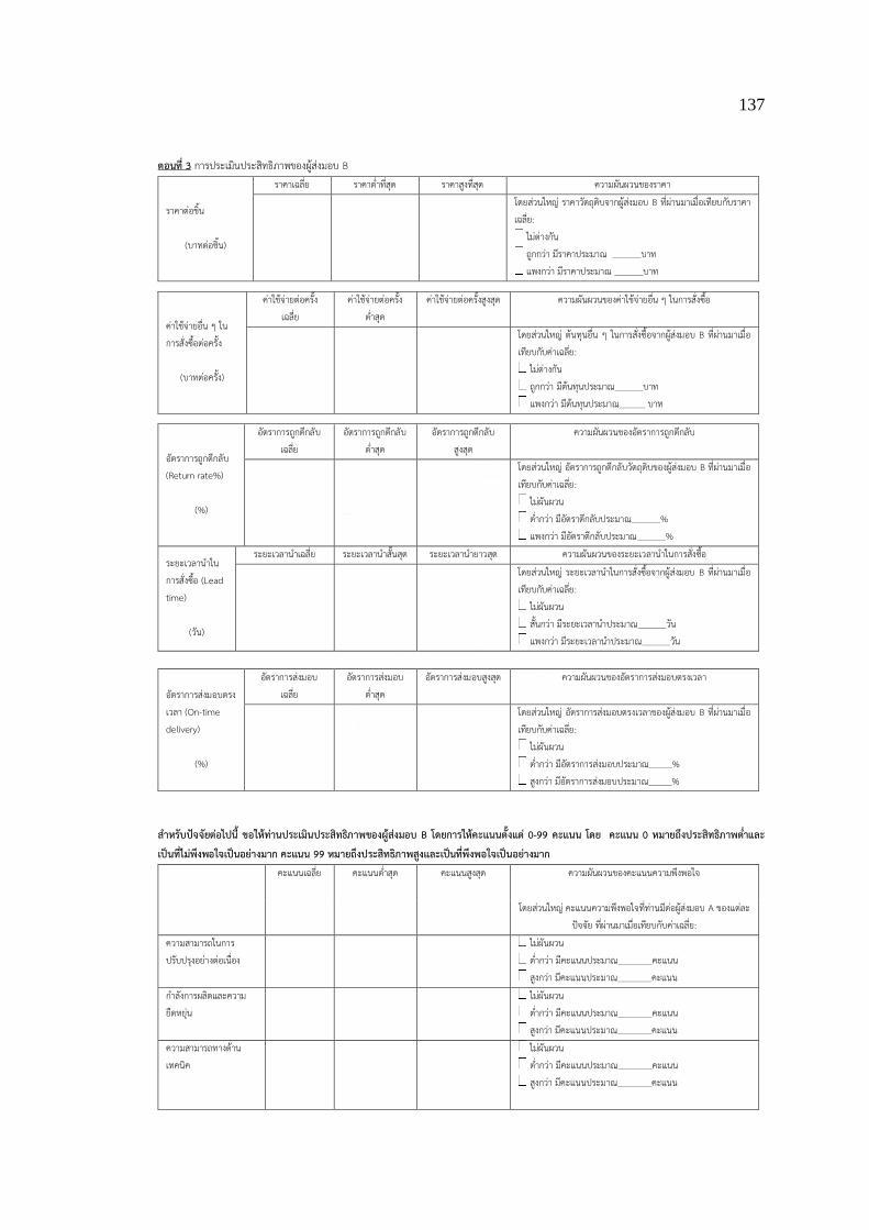
137
ตอนท 3 การประเมนประสทธภาพของผสงมอบ B
ราคาตอชน
(บาทตอชน)
ราคาเฉลย ราคาต าทสด ราคาสงทสด ความผนผวนของราคา โดยสวนใหญ ราคาวตถดบจากผสงมอบ B ทผานมาเมอเทยบกบราคา
เฉลย: ไมตางกน ถกกวา มราคาประมาณ บาท
แพงกวา มราคาประมาณ บาท
คาใชจายอน ๆ ในการสงซอตอครง
(บาทตอครง)
คาใชจายตอครงเฉลย
คาใชจายตอครงต าสด
คาใชจายตอครงสงสด ความผนผวนของคาใชจายอน ๆ ในการสงซอ
โดยสวนใหญ ตนทนอน ๆ ในการสงซอจากผสงมอบ B ทผานมาเมอเทยบกบคาเฉลย:
ไมตางกน ถกกวา มตนทนประมาณ บาท แพงกวา มตนทนประมาณ บาท
อตราการถกตกลบ (Return rate%)
(%)
อตราการถกตกลบเฉลย
อตราการถกตกลบต าสด
อตราการถกตกลบสงสด
ความผนผวนของอตราการถกตกลบ
โดยสวนใหญ อตราการถกตกลบวตถดบของผสงมอบ B ทผานมาเมอเทยบกบคาเฉลย:
ไมผนผวน ต ากวา มอตราตกลบประมาณ % แพงกวา มอตราตกลบประมาณ %
ระยะเวลาน าในการสงซอ (Lead time)
(วน)
ระยะเวลาน าเฉลย ระยะเวลาน าสนสด ระยะเวลาน ายาวสด ความผนผวนของระยะเวลาน าในการสงซอ
โดยสวนใหญ ระยะเวลาน าในการสงซอจากผสงมอบ B ทผานมาเมอเทยบกบคาเฉลย:
ไมผนผวน สนกวา มระยะเวลาน าประมาณ วน แพงกวา มระยะเวลาน าประมาณ วน
อตราการสงมอบตรงเวลา (On-time delivery)
(%)
อตราการสงมอบเฉลย
อตราการสงมอบต าสด
อตราการสงมอบสงสด ความผนผวนของอตราการสงมอบตรงเวลา
โดยสวนใหญ อตราการสงมอบตรงเวลาของผสงมอบ B ทผานมาเมอเทยบกบคาเฉลย:
ไมผนผวน ต ากวา มอตราการสงมอบประมาณ % สงกวา มอตราการสงมอบประมาณ %
สาหรบปจจยตอไปน ขอใหทานประเมนประสทธภาพของผสงมอบ B โดยการใหคะแนนตงแต 0-99 คะแนน โดย คะแนน 0 หมายถงประสทธภาพตาและเปนทไมพงพอใจเปนอยางมาก คะแนน 99 หมายถงประสทธภาพสงและเปนทพงพอใจเปนอยางมาก
คะแนนเฉลย คะแนนต าสด คะแนนสงสด ความผนผวนของคะแนนความพงพอใจ
โดยสวนใหญ คะแนนความพงพอใจททานมตอผสงมอบ A ของแตละปจจย ทผานมาเมอเทยบกบคาเฉลย:
ความสามารถในการปรบปรงอยางตอเนอง
ไมผนผวน ต ากวา มคะแนนประมาณ คะแนน สงกวา มคะแนนประมาณ คะแนน
ก าลงการผลตและความยดหยน
ไมผนผวน ต ากวา มคะแนนประมาณ คะแนน สงกวา มคะแนนประมาณ คะแนน
ความสามารถทางดานเทคนค
ไมผนผวน ต ากวา มคะแนนประมาณ คะแนน สงกวา มคะแนนประมาณ คะแนน

138
คะแนนเฉลย คะแนนต าสด คะแนนสงสด ความผนผวนของคะแนนความพงพอใจ
โดยสวนใหญ คะแนนความพงพอใจททานมตอผสงมอบ A ของแตละปจจย ทผานมาเมอเทยบกบคาเฉลย:
ความรวมมอในการพฒนา ไมผนผวน ต ากวา มคะแนนประมาณ คะแนน สงกวา มคะแนนประมาณ คะแนน
ความใสใจตอการผลตสเขยว
ไมผนผวน ต ากวา มคะแนนประมาณ คะแนน สงกวา มคะแนนประมาณ คะแนน
ความใสใจตอผลตภณฑและการออกแบบสเขยว
ไมผนผวน ต ากวา มคะแนนประมาณ คะแนน สงกวา มคะแนนประมาณ คะแนน
การรบมอกบความเสยงจากธรรมชาต
ไมผนผวน ต ากวา มคะแนนประมาณ คะแนน สงกวา มคะแนนประมาณ คะแนน
การรบมอกบความผดพลาดของบคคล
ไมผนผวน ต ากวา มคะแนนประมาณ คะแนน สงกวา มคะแนนประมาณ คะแนน

139
VITA
VITA
Ornicha Anuchitchanchai was born and raised in Chiang Rai. After
graduation from Samakkhiwitthayakhom School, she attended Chiang Mai
University and received her Bachelor of Industrial Engineering in 2001. She began
her career as production engineer at LTEC Ltd. in Northern Region Industrial Estate.
After working there for one and a half year, she resigned for further study at
Chulalongkorn University and earned Master's Degree in Industrial Engineering in
2006. She have been working as a lecturer in Industrial and Logistics Engineering
since then. She also had professional experiences in logistics consultant of Bureau
of Logistics, Department of Primary Industries and Mines for years.