previous page - eefocusdata.eefocus.com/myspace/0/942/bbs/1174163529/29c6d0e7.pdf · previous page....

BIBLIOGRAPHY

1. J. D. Kraus, Antennas since Hertz and Marconi, IEEE Trans.

Anten. Propag. AP-33:131–137 (Feb. 1985).

2. C. A. Balanis, Antenna Theory: Analysis and Design, Wiley,New York, 1997.

3. C. A. Balanis, Antenna theory: A review, Proc. IEEE 80:7–23(Jan. 1992).

4. Special issue on wireless communications, IEEE Trans. An-

ten. Propag. AP-46 (June 1998).

5. J. C. Liberti, Jr., and T. S. Rappaport, Smart Antennas forWireless Communications: IS-95 and Third Generation

CDMA Applications, Prentice-Hall PTR, Englewood Cliffs,NJ, 1999.

6. T. S. Rappaport, ed., Smart Antennas: Adaptive Arrays, Al-gorithms, & Wireless Position Location, IEEE, 1998.

7. S. Bellofiore, J. Foutz, R. Govindarajula, I. Bahceci, C. A. Bal-anis, A. S. Spanias, J. M. Capone, and T. M. Duman, Smartantenna system, analysis integration, and performance formobile ad-hoc networks (MANETs), IEEE Trans. Anten. Prop-ag. (special issue on wireless communications) 50(5):571–581(May 2002).

8. C. A. Balanis and A. C. Polycarpou, Antennas, in Encyclope-

dia of Telecommunications, Wiley, Hoboken, NJ, 2003, pp.179–188.

9. IEEE Standard Definitions of Terms for Antennas, IEEEStandard 145-1983, IEEE Trans. Anten. Propag. AP-31(PartII of two parts):5–29 (Nov. 1983).

10. C. A. Balanis, Advanced Engineering Electromagnetics, Wi-ley, New York, 1989.

11. Special issue on phased arrays, IEEE Trans. Anten. Propag.47(3) (March 1999).

12. Special issue on adaptive antennas, IEEE Trans. Anten. Prop-ag. AP-24 (Sept. 1976).

13. Special issue on adaptive processing antenna systems, IEEE

Trans. Anten. Propag. AP-34 (Sept. 1986).

ANTENNA RADIATION PATTERNS

MICHAEL T. CHRYSSOMALLIS

Democritus University ofThrace

Xanthi, Greece

CHRISTOS G.CHRISTODOULOU

The University of New MexicoAlbuquerque, New Mexico

1. ANTENNAS AND FUNDAMENTAL PARAMETERS

An antenna is used to either transmit or receive electro-magnetic waves. It serves as a transducer converting guid-ed waves into free-space waves in the transmitting modeor vice versa in the receiving mode. Antennas or aerialscan take many forms according to the radiation mecha-nism involved and can be divided in different categories.Some common types are wire antennas, aperture anten-nas, reflector antennas, lens antennas, traveling-wave an-tennas, frequency-independent antennas, horn antennas,

and printed and conformal antennas, [1, pp. 563–572].When applications require radiation characteristics thatcannot be met by a single radiating element, multiple el-ements are employed. Various configurations are utilizedby suitably spacing the elements in one or two dimensions.These configurations, known as array antennas, can pro-duce the desired radiation characteristics by appropriatelyfeeding each individual element with different amplitudesand phases that allows a mechanism for increasing theelectric size of the antenna. Furthermore, antenna arrayscombined with signal processing lead to smart antennas(switched-beam or adaptive antennas) that offer moredegrees of freedom in the wireless system design [2].Moreover, active antenna elements or arrays incorporatesolid-state components producing effective integratedantenna transmitters or receivers with many applications[1, pp. 190–209; 2].

Regardless of the antenna considered, certain funda-mental figures of merit describe the performance of anantenna. The response of an antenna as a function of di-rection is given by the antenna pattern. This pattern com-monly consists of a number of lobes, where the largest oneis called the mainlobe and the others are referred to assidelobes, minorlobes, or backlobes. If the pattern is mea-sured sufficiently far from the antenna so there is nochange in the pattern with distance, the pattern is theso called ‘far-field pattern’. Measurements at shorter dis-tances yield ‘near-field patterns’, which are a function ofboth angle and distance. The pattern may be expressed interms of the field intensity, called field pattern, or in termsof the Poynting vector or radiation intensity, which areknown as power patterns. If the pattern is symmetric,a simple pattern is sufficient to completely specify thevariation of the radiation with the angle. Otherwise, athree-dimensional diagram or a contour map is required toshow the pattern in its entirety. However, in practice, twopatterns perpendicular to each other and perpendicular tothe mainlobe axis may suffice. These are called the ‘prin-cipal-plane’ patterns, the E plane and the H plane, con-taining the E and H field vectors, respectively. Havingestablished the radiation patterns of an antenna, someimportant parameters can now be considered such as ra-diated power, radiation efficiency, directivity, gain, andantenna polarization. All of them are considered in detailin this article.

Here, scalar quantities are presented in italics, whilevector quantities are in boldface, for example, electric fieldE (vector) of E(¼|E|) (scalar). Unit vectors are boldfacewith a circumflex over the letter; xx, yy, zz, and rr are the unitvectors in x, y, z, and r directions, respectively. A dot overthe symbol means that the quantity is harmonically time-varying or a phasor. For example, taking the electric field,.E represents a space vector and time phasor, but

.Ex is a

scalar phasor. The relations between them are.E¼ xx

.Ex

where.

Ex¼E1ejot.The first section of this article introduces several

antenna patterns, giving the necessary definitions andpresenting the common types. The field regions of anantenna are also pointed out. The most common referenceantennas are the ideal isotropic radiator and the veryshort dipole. Their fields are used to show the calculation

ANTENNA RADIATION PATTERNS 225

Previous Page

and meaning of the different parameters of antennas cov-ered in this article. The second section begins with a treat-ment of the Poynting vector and radiation power density,starting from the general case of an electromagnetic waveand extending the definitions to a radiating antenna. Afterthis, radiation performance measures such that the beamsolid angle, directivity, and gain of an antenna are defined.In the third section the concepts of wave and antenna po-larization are discussed. Finally, in the fourth section, ageneral case of antenna pattern calculation is considered,and numerical solutions are suggested for radiationpatterns that are not available in simple closed-formexpressions.

2. RADIATION FROM ANTENNAS

2.1. Radiation Patterns

The radiation pattern of an antenna is, generally, its mostbasic requirement since it determines the spatial distri-bution of the radiated energy. This is usually the firstproperty of an antenna that is specified, once the operat-ing frequency has been stated. An antenna radiation pat-tern or antenna pattern is defined as a graphicalrepresentation of the radiation properties of the antennaas a function of space coordinates. Since antennas arecommonly used as parts of wireless telecommunicationsystems, the radiation pattern is determined in the far-field region where no change in pattern with distance oc-curs. Using a spherical coordinate system, shown in Fig. 1,where the antenna is at the origin, the radiation proper-ties of the antenna depend only on the angles f and yalong a path or surface of constant radius. A trace of theradiated or received power at a constant radius is called apower pattern, while the spatial variation of the electric ormagnetic field along a constant radius is called an ampli-tude field pattern. In practice, the necessary informationfrom the complete three-dimensional pattern of an anten-na can be received by taking a few two-dimensionalpatterns, according to the complexity of radiation patternof the specific antenna. Usually, for most applications, anumber of plots of the pattern as a function of y for someparticular values off, plus a few plots as a function off forsome particular values of y, give the needed information.

Antennas usually behave as reciprocal devices. This isvery important since it permits the characterization of theantenna as either a transmitting or receiving antenna. Forexample, radiation patterns are often measured with thetest antenna operating in the receive mode. If the antennais reciprocal, the measured pattern is identical when theantenna is in either a transmit or a receive mode. If non-reciprocal materials, such as ferrites and active devices,are not present in an antenna, its transmitting and re-ceiving properties are identical.

The radiation fields from a transmitting antenna varyinversely with distance, while the variation with observa-tion angles (f, y) depends on the antenna type. A very sim-ple but basic configuration antenna is the ideal or very shortdipole antenna. Since any linear or curved wire antennamay be regarded, as being composed of a number of shortdipoles connected in series, the knowledge of this antenna is

useful. So, we will use the fields radiated from an ideal an-tenna to define and understand the radiation pattern prop-erties. An ideal dipole positioned symmetrically, at theorigin of the coordinate system and oriented along the zaxis, is shown in Fig. 1. The pattern of electromagneticfields, with wavelength l, around a very short wire antennaof length L5l, carrying a uniform current I0e

jot, is de-scribed by functions of distance, frequency, and angle. Table1 summarizes the expressions for the fields from a veryshort dipole antenna as [3,4] Ej¼Hr¼Hy¼ 0 for rbl andL5l. The variables shown in these relations are as follows:I0¼ amplitude (peak value in time) of current (A), assumedto be constant along the dipole; L¼ length of dipole (m); o¼2pf¼ radian frequency, where f is the frequency in Hz; t¼time (s); b¼ 2p/l¼phase constant (rad/m); y¼ azimuthalangle (dimensionless); c¼ velocity of light E3� 108 m/s; l¼wavelength (m); j¼ complex operator¼

ffiffiffiffiffiffiffi�1p

; r¼distancefrom center of dipole to observation point (m); and e0¼per-mittivity of free space¼ 8.85 pF/m.

It is to be noted that Ey and Hf are in time phase in thefar field. Thus, electric and magnetic fields in the far fieldof the spherical wave from the dipole are related in thesame manner as in a plane traveling wave. Both are alsoproportional to sin y; that is, both are maximum when y¼901 and minimum when y¼ 01 (in the direction of the di-pole axis). This variation of Ey or Hf with angle can bepresented by a field pattern (shown in Fig. 2), where thelength r of the radius vector is proportional to the value ofthe far field (Ey or Hf) in that direction from the dipole.The pattern in Fig. 2a is the three-dimensional far-fieldpattern for the ideal dipole, while the patterns in Figs. 2band 2c are two-dimensional and represent cross sections ofthe three-dimensional pattern, showing the dependence ofthe fields with respect to angles y and f.

All far-field components of a very short dipole are func-tions of I0, the dipole current; L/l, the dipole length interms of wavelengths; 1/r, the distance factor; jej(ot–br), thephase factor; and sin y, the pattern factor that gives thevariation of the field with angle. In general, the expressionfor the field of any antenna will involve these factors.

�

Azimuth plane

Elevation plane

�

x

y

z

L

E�

E�

Er

r

Figure 1. Spherical coordinate system for antenna analysis pur-poses. A very short dipole is shown with its no-zero field compo-nent directions.

226 ANTENNA RADIATION PATTERNS

For longer antennas with complicated current distri-bution, the field components generally are functions of theterms defined above, which are grouped and designated asthe element factor and the space factor. The element factorincludes everything except the current distribution alongthe source, which is the space factor of the antenna. If, forexample, we consider the case of a finite dipole antenna,we can produce the field expressions by dividing the an-tenna into a number of very short dipoles and summing allthe contributions. The element factor is equal to the fieldof the very short dipole located at a reference point, whilethe space factor is a function of the current distributionalong the source, the latter usually described by an inte-gral. The total field of the antenna is taken by the productof the element and space factors. This procedure is knownas pattern multiplication.

A similar procedure is used in array antennas, whichare used when it is necessary to design antennas with di-rective characteristics. The increased electrical size of anarray antenna due to the use of more than one radiating

elements gives better directivity and special radiation pat-terns. The total field of an array is determined by theproduct of the field of a single element and the array factorof the array antenna. If we use isotropic radiating ele-ments, the pattern of the array is simply the pattern of thearray factor. The array factor is a function of the geometryof the array and the excitation phase. Thus, changing thenumber of elements, their geometric arrangement, theirrelative magnitudes, their relative phases, and their spac-ing, we take different patterns. Figure 3 shows some casesof characteristic patterns of an array antenna with twoisotropic point sources as radiating elements, by usingdifferent values of the above mentioned quantities, whichproduce different array factors.

2.2. Common Types of Radiation Patterns

An isotropic source or radiator is an ideal antenna thatradiates uniformly in all directions in space. Although nopractical source has this property, the concept of the iso-

Table 1. Fields of an Ideal or Very Short Dipole

Component General Expression for All regions Far Field Only

ErI0 Le jðot�brÞ cos y

joe04pr2jbrþ

2

r2

� �0

Ey �I0 Le jðot�brÞ sin y

joe04prb2�

jbr�

1

r2

� �jðL=lÞI0e jðot�brÞ sin y

2e0cr

HfI0 Le jðot�brÞ sin y

4prjbþ

1

r

� �jðL=lÞI0e jðot�brÞ sin y

2r

x

y

�

z

�

HPBW= 90°

sin �

x

z

y

(b) (c)

(a)

Figure 2. Radiation field pattern of far field from anideal or very short dipole: (a) three-dimensional pat-tern plot; (b) E-plane radiation pattern polar plot;(c) H-plane radiation pattern polar plot.


tropic radiator is very useful and is often used as a refer-ence for expressing the directive properties of actual an-tennas. It is worth recalling that the power flux density Sat a distance r from an isotropic radiator is Pt/4pr2, wherePt is the transmitted power, since all the transmitted pow-er is evenly distributed on the surface of a spherical wave-front with radius r. The electric field intensity iscalculated as

ffiffiffiffiffiffiffiffiffiffi30Pt

p=r (using the relation from electric

circuits, power¼E2/Z, where Z¼ the characteristic imped-ance of free space¼ 377O).

On the contrary, a directional antenna is one that ra-diates or receives electromagnetic waves more effectivelyin some directions than in others. An example of an an-tenna with a directional radiation pattern is that of anideal or very short dipole, shown in Fig. 2. It is seen thatthis pattern, which resembles a doughnut with no hole, isnondirectional in the azimuth plane, which is the xy planecharacterized by the set of relations [ f (f), y¼ p/2], anddirectional in the elevation plane, which is any orthogonalplane containing the z axis characterized by [ g(y), f¼constant]. This type of directional pattern is designated asan omnidirectional pattern and is defined as one havingan essentially nondirectional pattern in a given plane,which for this case is the azimuth plane and a directional

pattern in any orthogonal plane, in this case the elevationplane. The omnidirectional pattern—also known as broad-cast-type—is used for many broadcast or communicationsservices where all directions are to be covered equallywell. The horizontal-plane pattern is generally circular,while the vertical-plane pattern may have some directiv-ity in order to increase the gain.

Other forms of directional patterns are pencil-beam,fan-beam, and shaped-beam patterns. The pencil-beampattern is a highly directional pattern that is used to ob-tain maximum gain and when the radiation pattern is tobe concentrated in as narrow an angular sector as possi-ble. The beamwidths in the two principal planes are es-sentially equal. The fan-beam pattern is similar to thepencil-beam pattern except that the beam cross section iselliptical in shape rather than circular. The beamwidth inone plane may be considerably broader than the beam-width in the other plane. As with the pencil-beam pattern,the fan-beam pattern generally implies a rather substan-tial amount of gain. The shaped-beam pattern is usedwhen the pattern in one of the principal planes must pref-erably have a specified type of coverage. A typical exampleis the cosecant type of pattern, which is used to provide aconstant radar return over a range of angles in the

Distance = 0.5� Phase = 180°


Distance = 0.25�Phase = 180°


(c)

(d)

(a)

(b)

Figure 3. Three-dimensional graphs of power radiation patterns for an array of two isotropicelements of the same amplitude and (a) opposite phase, spaced 0.5l apart; (b) phase quadrature,spaced 0.5l apart; (c) opposite phase, spaced 0.25l apart; and (d) opposite phase, spaced 1.5l, apart.


vertical plane. The pattern in the other principal plane isusually a pencil-beam pattern but may sometimesbe a circular pattern as in certain types of beacon anten-nas. In addition to these pattern types, there are a numberof pattern shapes used for direction finding and otherpurposes that do not fall under the categories alreadymentioned. These patterns include the well-knownfigure-of-eight pattern, the cardioid pattern, split-beampatterns, and multilobed patterns whose lobes are ofsubstantially equal amplitude. For those patterns, whichhave particularly unusual characteristics, it is generallynecessary to specify the pattern by an actual plot of itsshape or by the mathematical relationship that describesits shape.

Antennas are often referred to by the type of patternthey produce. Two terms that usually characterize arrayantennas, are broadside and endfire. A broadside antennais one for which the mainbeam maximum is in a directionnormal to the plane containing the antenna. An endfireantenna is one for which the mainbeam is in the planecontaining the antenna. For example, the short dipole an-tenna is a broadside antenna. Figure 4 shows the twocases of broadside and endfire radiation patterns, whichare produced from a linear uniform array of isotropicsources of 0.5 wavelength spacing, between adjacent ele-ments. The type of radiation pattern is controlled by thechoice of phase shift angle between the elements. Zerophase shift produces a broadside pattern and 1801 phaseshift leads to an endfire pattern, while intermediatevalues produce radiation patterns with the mainlobesbetween these two cases.

2.3. Characteristics of Simple Patterns

For a linearly polarized antenna, as a very short dipoleantenna, performance is often described in terms of twopatterns (Figs. 2b and 2c). Any plane containing the z-axishas the same radiation pattern since there is no variationin the fields with angle f (Fig. 2b). A pattern taken in oneof these planes is called an E-plane pattern because it isparallel to the electric field vector E and passes throughthe antenna in the direction of the beam maximum. A

pattern taken in a plane orthogonal to an E plane andcutting through the short dipole antenna, the xy plane inthis case, is called an H-plane pattern because it containsthe magnetic field H and also passes through the antennain the direction of the beam maximum (Fig. 2c). TheE- and H-plane patterns, in general, are referred to asthe principal-plane patterns. The pattern plots in Figs. 2band 2c are called polar patterns or polar diagrams. Formost types of antennas it is a usual practice to orient themso that at least one of the principal-plane patterns coin-cides with one of the geometric principal planes. This isillustrated in Fig. 5, where the principal planes of a mi-crostrip antenna are plotted. The xy plane (azimuthalplane, y¼ p/2) is the principal E plane, and the xz plane(elevation plane, f¼0) is the principal H plane.

A typical antenna power pattern is shown in Fig. 6. InFig. 6a depicts a polar plot in linear scale; Fig. 6b showsthe same pattern in rectangular coordinates in decibels.As can be seen, the radiation pattern of the antenna con-sists of various parts, which are known as lobes. Themainlobe (or mainbeam or major lobe) is defined as thelobe containing the direction of maximum radiation. InFig. 6a the mainlobe is pointing in the y¼0 direction. Insome antennas there may exist more than one major lobe.A minor lobe is any lobe except the mainlobe. Minor lobesare composed of sidelobes and backlobes. The term side-lobe is sometimes reserved for those minor lobes near themainlobe but is most often taken to be synonymous withminor lobe. A backlobe is a radiation lobe in, approximate-ly, the opposite direction to the mainlobe. Minor lobesusually represent radiation in undesired directions, andthey should be minimized. Sidelobes are normally thelargest of the minor lobes. The level of side or minor lobesis usually expressed as a ratio of the power density in thelobe in question to that of the mainlobe. This ratio is oftentermed the sidelobe ratio or sidelobe level, and desiredvalues depend on the antenna application.

For antennas with simple shape patterns, the half-power beamwidth and sidelobe level in the two principalplanes specify the important characteristics of the

(a) (b)

Figure 4. Polar plots of a linear uniform amplitude array of fiveisotropic sources with 0.5l spacing between the sources: (a) broad-side radiation pattern (01 phase shift between successive ele-ments); (b) endfire radiation pattern (1801 phase shift).

E − plane

H − plane

x z

y

Figure 5. The principal plane patterns of a microstrip antenna:(a) the xy plane or E-plane (azimuth plane, y¼p/2) and (b) the xz

plane or H plane (elevation plane, f¼0).


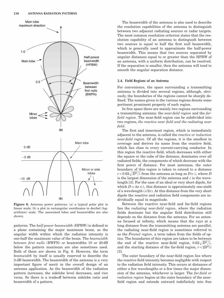
patterns. The half-power beamwidth (HPBW) is defined ina plane containing the major maximum beam, as theangular width within which the radiation intensity isone-half the maximum value of the beam. The beamwidthbetween first nulls (BWFN) or beamwidths 10 or 20 dBbelow the pattern maximum are also sometimes used.Both of them are shown in Fig. 6. However, the termbeamwidth by itself is usually reserved to describe the3-dB beamwidth. The beamwidth of the antenna is a veryimportant figure of merit in the overall design of anantenna application. As the beamwidth of the radiationpattern increases, the sidelobe level decreases, and viceversa. So there is a tradeoff between sidelobe ratio andbeamwidth of a pattern.

The beamwidth of the antenna is also used to describethe resolution capabilities of the antenna to distinguishbetween two adjacent radiating sources or radar targets.The most common resolution criterion states that the res-olution capability of an antenna to distinguish betweentwo sources is equal to half the first null beamwidth,which is generally used to approximate the half-powerbeamwidth. This means that two sources separated byangular distances equal to or greater than the HPBW ofan antenna, with a uniform distribution, can be resolved.If the separation is smaller, then the antenna will tend tosmooth the angular separation distance.

2.4. Field Regions of an Antenna

For convenience, the space surrounding a transmittingantenna is divided into several regions, although, obvi-ously, the boundaries of the regions cannot be sharply de-fined. The names given to the various regions denote somepertinent prominent property of each region.

In free space there are mainly two regions surroundinga transmitting antenna: the near-field region and the far-field region. The near-field region can be subdivided intotwo regions, the reactive near field and the radiating nearfield.

The first and innermost region, which is immediatelyadjacent to the antenna, is called the reactive or inductionnear-field region. Of all the regions, it is the smallest incoverage and derives its name from the reactive field,which lies close to every current-carrying conductor. Inthis region the reactive field, which decreases with eitherthe square or the cube of the distance, dominates over allradiated fields, the components of which decrease with thefirst power of distance. For most antennas, the outerboundary of this region is taken to extend to a distancero0:62

ffiffiffiffiffiffiffiffiffiffiffiD3=l

pfrom the antenna as long as Dbl, where D

is the largest dimension of the antenna and l is the wave-length [3]. For the case of an ideal or very short dipole, forwhich D¼Dz5l, this distance is approximately one-sixthof a wavelength (l/2p). At this distance from the very shortdipole the reactive and radiation field components are in-dividually equal in magnitude.

Between the reactive near-field and far-field regionslies the radiating near-field region, where the radiationfields dominate but the angular field distribution stilldepends on the distance from the antenna. For an anten-na focused at infinity, which means that the rays at along distance from the transmitting antenna are parallel,the radiating near-field region is sometimes referred toas the Fresnel region, a term taken from the fields of op-tics. The boundaries of this region are taken to be betweenthe end of the reactive near-field region, 0:62


p,

and the starting distance of the far-field region, ro2D2/l[3].

The outer boundary of the near-field region lies wherethe reactive field intensity becomes negligible with respectto the radiation field intensity. This occurs at distances ofeither a few wavelengths or a few times the major dimen-sion of the antenna, whichever is larger. The far-field orradiation region begins at the outer boundary of the near-field region and extends outward indefinitely into free

Minor or side lobes

0 dB

−3 dB

−10 dB

Main lobe

(a)

(b)

Figure 6. Antenna power patterns: (a) a typical polar plot inlinear scale; (b) a plot in rectangular coordinates in decibel (log-arithmic) scale. The associated lobes and beamwidths are alsoshown.


space. In this region the angular field distribution of thefield of the antenna is essentially independent of thedistance from the antenna. For example, for the caseof a very short dipole, the sin y pattern dependence isvalid anywhere in this region. The far-field region iscommonly taken to exist at distances r42D2/l from theantenna, and for an antenna focused at infinity it issometimes referred to as the Fraunhofer region. All threeregions surrounding an antenna and their boundaries areillustrated in Fig. 7.

3. ANTENNA PERFORMANCE MEASURES

3.1. Poynting Vector and Radiation Power Density

In an electromagnetic wave, electric and magnetic ener-gies are stored in equal amounts in the electric andmagnetic fields, which together constitute the wave. Thepower flow is found by making use of the Poynting vectorS, defined as

S¼E�H ð1Þ

where E(V/m) and H(A/m) are the field vectors. Sincethe Poynting vector represents a surface power density(W/m2), the integral of its normal component over aclosed surface always gives the total power through thesurface IZ

A

S .dA¼P ð2Þ

where P is the total power (W) flowing out of closed surfaceA and dA¼ nndA, where nn is the unit vector normal to thesurface. The Poynting vector S and the power P in therelations above are instantaneous values.

Normally, it is the time-averaged Poynting vector Sav,which represents the average power density, that is of

practical interest, and is given by

Sav¼1

2Reð

.E�

.H�Þ ðW=m2Þ ð3Þ

where the term Re stands for the real part of the complexnumber and the asterisk � denotes the complex conjugate.Note that

.E and

.H in Eq. (3) are respectively the expres-

sions for the electric and magnetic fields written as com-plex numbers to include the change with time. Thus, for aplane wave traveling in the positive z direction with elec-tric and magnetic field components in x and y directions,respectively, the electric field is E¼ xxEx0ejot, while inEq. (1) it is E¼ xxEx0. The 1

2 factor appears because thefields represent peak values and should be omitted forRMS (root-mean-square) values.

The average power Pav flowing outward through aclosed surface can now be obtained by integratingEq. (3):

Pav¼

IZA

Re.S .dA¼

1

2

IZA

Reð.E�

.H�Þ .dA¼Prad ðWÞ ð4Þ

Consider the case where the electromagnetic wave is ra-diated by an antenna. If the closed surface is taken aroundthe antenna within the far-field region, then this integra-tion results in the average power radiated by the antenna.This is called radiation power Prad, while Eq. (3) repre-sents the radiation power density Sav of the antenna.The imaginary part of Eq. (3) represents the reactivepower density stored in the near field of an antenna. Sincethe electromagnetic fields of an antenna in its far-field re-gion are predominately real, Eq. (3) suffices for ourpurposes.

The average power density radiated by the antenna asa function of direction, taken on a large sphere of constantradius in the far-field region, results in the power pattern

2D2/�

Radiating region

Near field region Far field region

Reactive region

0.62

D

D 3/�

Figure 7. Field regions of an antenna and somecommonly used boundaries.


of the antenna. As an example, for an isotropic radiator,the total radiation power is given by

Prad¼

ZZA

Si .dA¼

Z 2p

0

Z p

0½rrSiðrÞ� . ½rrr2 sin y dydf�

¼ 4pr2Si

ð5Þ

where, because of symmetry, the Poynting vectorSi¼ rrSiðrÞ is taken independent of the spherical coordi-nate angles y and f, having only a radial component.

From Eq. (5) the power density can be found:

Si¼ rrSi¼ rrPrad

4pr2

� �ðW=m2Þ ð6Þ

This result can also be reached if we assume that the ra-diated power expands radially in all directions with thesame velocity and is evenly distributed on the surface of aspherical wavefront of radius r.

As we will see later, an electromagnetic wave may havean electric field consisting of two orthogonal linear com-ponents of different amplitudes, Ex0 and Ey0, respectively,and a phase angle between of them d. Thus, the total elec-tric field vector, called an elliptically polarized vector,becomes

.E¼ xx

.Exþ yy

.Ey¼ xxEx0e jðot�bzÞ þ yyEy0eð jðot�bzþ dÞ ð7Þ

which at z¼0 becomes.E¼ xx

.Exþ yy

.Ey¼ xxEx0e jotþ yyEy0e jðotþ dÞ ð8Þ

So.E is a complex vector (phasor vector) that is resolvable

into two components xx.

Ex and yy.

Ey. The total.

H field vectorassociated with

.E at z¼ 0 is then

.H¼ yy

.Hy � xx

.Hx¼ yyHy0e jðot�zÞ � xxHx0e jðotþ d�zÞ ð9Þ

where z is the phase lag of.

Hy with respect to.

Ex. From Eq.(9) the complex conjugate magnetic field can be foundchanging only the sign of exponents.

Now the average Poynting vector can be calculated us-ing the fields defined above:

Sav¼1

2Re½ðxx� yyÞ

.Ex

.H�

y � ðyy� xxÞ.

Ey

.H�

x�

¼1

2zzReð

.Ex

.H�

y þ.

Ey

.H�

xÞ

¼1

2zzReðEx0Hx0þEy0Hy0Þ cos z

ð10Þ

It should be noted that Sav is independent of d, the phaseangle between the electric field components.

In a lossless medium, z¼ 0, because electric and mag-netic fields are in time phase and Ex0/Hx0¼Ey0/Hy0¼ Z,where Z, is the intrinsic impedance of the medium that is

real. If E¼ffiffiffiffiffiffiffiffiffiffiffiffiffiffiffiffiffiffiffiffiE2

x0þE2y0

qand H¼

ffiffiffiffiffiffiffiffiffiffiffiffiffiffiffiffiffiffiffiffiffiH2

x0þH2y0

qare the am-

plitudes of the total E and H fields, respectively, then

Sav¼1

2zz

E2x0þE2

y0

Z¼

1

2zz

E2

Z

¼1

2zzðH2

x0þH2y0ÞZ¼

1

2zzH2Z

ð11Þ

These expressions are the most general form of radiationpower density of an elliptically polarized wave or of an el-liptically polarized antenna, respectively, and hold for allcases, including the linear and circular polarization cases,which will introduce later on.

3.2. Radiation Intensity

Radiation intensity is a far-field parameter, in termsof which any antenna radiation power pattern can be de-termined. Thus, the antenna power pattern, as a functionof angle, can be expressed in terms of its radiationintensity as [3]:

Uðy;fÞ¼Savr2

¼r2

2ZjEðr; y;fÞj2

¼r2

2ZjEyðr; y;fÞj2þ jEfðr; y;fÞj2� �

�1

2ZjEyðy;fÞj2þ jEfðy;fÞj2� �

ð12Þ

where

U(y, f)¼ radiation intensity (W/unit solid angle)Sav ¼ radiation density or radial component of Poyn-

ting vector (W/m2)E(r, y, f) ¼ total transverse electric field (V/m)H(r, y, f)¼ total transverse magnetic field (A/m)

r¼distance from antenna to point of measure-ment (m)

Z ¼ intrinsic impedance of medium (O per square)

In Eq. (12) the electric and magnetic field are expressed interms of spherical coordinates.

What makes radiation intensity important is that it isindependent of distance. This is because in the far field thePoynting vector is entirely radial, which means that thefields are entirely transverse and E and H vary as 1/r.

Since the radiation intensity is a function of angle, itcan also be defined as the power radiated from an antennaper unit solid angle. The measure of a solid angle is thesteradian. One steradian is described as the solid anglewith its vertex at the center of a sphere that has radius r,which is subtended by a spherical surface area equivalentto that of a square of size r2. But the area of a sphere ofradius r is given by A¼ 4pr2, so in a closed sphere thereare 4pr2/r2

¼ 4p sr. For a sphere of radius r, an infinites-imal area dA on its surface can be written as

dA¼ r2 sin ydydf ðm2Þ ð13Þ

and therefore the element of solid angle dO of a sphere isgiven by

dO¼dA

r2¼ sin ydydf ðsrÞ ð14Þ

Thus, the total power can be obtained by integrating theradiation intensity, as given by Eq. (12), over the entire


solid angle of 4p, as

Prad¼

IZO

Uðy;fÞdO¼Z 2p

0

Z p

0Uðy;fÞ sin ydydf ð15Þ

As an example, for the isotropic radiator ideal antenna,the radiation intensity U(y,f) will be independent of theangles y and f and the total radiated power will be

Prad¼

IZO

UidO¼Ui

Z 2p

0

Z p

0

sin ydydf

¼Ui

IZO

dO¼ 4pUi

ð16Þ

or Ui¼Prad/4p, which is the power density of Eq. (6) mul-tiplied by r2.

Dividing U(y,f) by its maximum value Umax(y,f), weobtain the normalized antenna power pattern:

Unðy;fÞ¼Uðy;fÞ

Umaxðy;fÞðdimensionlessÞ ð17Þ

A term associated with the normalized power pattern isthe beam solid angle. The beam solid angle OA is definedas the angle through which all the power from a radiatingantenna would flow if the power per unit solid angle wereconstant over this angle and equal to its maximum value(Fig. 8). This means that, for typical patterns, the solidbeam angle is approximately equal to the half-power beamwidth (HPBW):

OA¼

Z 2p

0

Z p

0

Unðy;fÞ sin ydydf¼IZ

4pUnðy;fÞdO ðsrÞ

ð18Þ

If the integration is done over the mainlobe, the mainlobesolid angle, OM, is defined, and the difference of OA�OM

gives the minor-lobe solid angle. These definitions hold forpatterns with clearly defined lobes. The beam efficiency(BE) of an antenna is defined as the ratio of OM/OA and is ameasure of the amount of power in the major lobe com-pared to the total power. A high beam efficiency meansthat most of the power is concentrated in the major lobeand that minor lobes are minimized.

3.3. Directivity and Gain

A very important antenna parameter that indicates howwell an antenna concentrates power into a limited solidangle is its directivity D. The directivity of an antenna isdefined as the ratio of the maximum radiation intensity tothe radiation intensity averaged over all directions. Theaverage radiation intensity is calculated by dividing thetotal power radiated by 4p sr. Hence

D¼Umaxðy;fÞ

Uav¼

Umaxðy;fÞUi

¼Umaxðy;fÞPrad=4p

¼4pUmaxðy;fÞ

PradðdimensionlessÞ

ð19Þ

since from Eq. (16), Prad/4p¼Ui. So, alternatively, the di-rectivity of an antenna can be defined as the ratio of itsradiation intensity in a given direction, which usually istaken to be the direction of maximum radiation intensity,divided by the radiation intensity of an isotropic sourcewith the same total radiation intensity. Equation (19) canalso be written

D¼Umaxðy;fÞPrad=4p

¼4pUmaxðy;fÞIZ

4pUðy;fÞdO

¼4pIZ

4pUðy;fÞ=Umaxðy;fÞdO

¼4pIZ

4pUnðy;fÞdO

¼4pOA

ð20Þ

Thus, the directivity of an antenna is equal to the solidangle of a sphere, which is 4p sr, divided by the antennabeam solid angle OA. We can say that by this relation thevalue of directivity is derived from the antenna pattern. Itis obvious from this relation that the smaller the beamsolid angle, the larger the directivity, or stated in a differ-ent way, an antenna that concentrates its power in a nar-row mainlobe has a great value of directivity.

Obviously, the directivity of an isotropic antenna isunity. By definition, an isotropic source radiates equallyin all directions. If we use Eq. (20), then OA¼ 4p sinceUn(y, f)¼ 1. This is the smallest directivity value that onecan attain. However, if we consider the directivity in aspecified direction, for example, D(y,f) its value can besmaller than unity. As an example, let us calculate the

Half-power Beamwidth

(HPBW)

Figure 8. Power pattern and beam solid angle of an antenna.


directivity of the very short dipole antenna. We cancalculate its normalized radiated power using the electricor the magnetic field components, given in Table 1. Usingthe electric field Ey for far-field region, from Eq. (12), wehave

Unðy;fÞ¼Uðy;fÞ

Umaxðy;fÞ¼

E2yðy;fÞ

½E2yðy;fÞ�max

¼ sin2 y ð21Þ

and

D¼4pIZ

4pUnðy;fÞdO

¼4pZ 2p

0

Z p

0sin3 ydydf

¼3

2¼ 1:5

ð22Þ

Alternatively, we can work using power densities insteadof power intensities. The power flowing in a particulardirection can be calculated using Eq. (3) and using theelectric and magnetic far-field components given inTable 1:

Sav¼Z2

I0Lb4pr

� �2

sin2 y ðW=m2Þ ð23Þ

By integrating over all angles the total power flowing out-ward is given by

PT ¼Z

12pðI0LbÞ2 ðWÞ ð24Þ

The directivity of a very short dipole antenna can be foundfrom the ratio of the maximum power density to the av-erage power density. For the very short dipole antenna,the maximum power density is in the y¼901 direction(Fig. 2) and the average power density is found by aver-aging the total power PT from Eq. (24) over a sphere ofsurface area 4pr2:

D¼Sav

PT=4pr2¼ðZ=2ÞðI0Lb=4prÞ2

ðZ=12pÞðI0LbÞ2=4pr2¼

3

2ð25Þ

Thus, the directivity of a very short dipole is 1.5, whichmeans that the maximum radiation intensity is 1.5 timesthe power of the isotropic radiator. This is often expressedin decibels, such that

D¼ 10 log10ðdÞ dB¼ 10 log10ð1:5Þ¼ 1:76 dB ð26Þ

Here, we use small (lowercase) letters to indicate absolutevalue and capital (uppercase) letters for the logarithmicvalue of the directivity, which is a common symbolism inthe field of antennas and propagation.

In some cases it is convenient to use simpler expres-sions for directivity estimation instead of the exact ones.For antennas characterized by a radiation pattern con-sisting of one narrow mainlobe and negligible minorlobes, the beam solid angle can be approximated by theproduct of the half-power beamwidths in two perpendi-cular planes, and the directivity can be given by theexpression

D¼4pOA�

4pY1rY2r

¼41;253

Y1dY2dð27Þ

where Y1r, Y2r and Y1d, Y2d are the half-power beam-widths in two perpendicular planes in radians and de-grees, respectively.

The gain of an antenna is another basic property in thetotal characterization of an antenna. Gain is closely asso-ciated with directivity, which is dependent on the radia-tion patterns of an antenna. The gain is commonly definedas the ratio of the maximum radiation intensity in a givendirection to the maximum radiation intensity produced inthe same direction from a reference antenna with the samepower input. Any convenient type of antenna may be tak-en as a reference antenna. Often the type of the referenceantenna is dictated by the application area, but the mostcommonly used one is the isotropic radiator, the hypothet-ical lossless antenna with uniform radiation intensity inall directions. So

G¼Umaxðy;fÞ

Ui¼

Umaxðy;fÞPin=4p

ðdimensionlessÞ ð28Þ

where the radiation intensity of the reference antenna ofisotropic radiator is equal to the power in the input Pin ofthe antenna divided by 4p.

Real antennas are not lossless, which means that ifthey accept an input power Pin, the radiated power Prad

generally will less be than Pin. The antenna efficiency k isdefined as the ratio of these two powers

k¼Prad

Pin¼

Rr

RrþRlossðdimesionlessÞ ð29Þ

where Rr is the radiation resistance of the antenna. Rr isdefined as an equivalent resistance in which the samecurrent flowing at the antenna terminals will producepower equal to that produced by the antenna. Rloss isthe loss resistance that comes from any heat loss due to thefinite conductivity of the materials used to construct theantenna or due to losses associated by the dielectric struc-ture of the antenna. So, for a real antenna with losses, itsradiation intensity at a given direction U(y,f) will be

Uðy;fÞ¼ kU0ðy;fÞ ð30Þ

where U0(y, f) is the radiation intensity of the same an-tenna with no losses.

Substituting Eq. (30) into (28) yields the definition ofgain in terms of the antenna directivity:

G¼Umaxðy;fÞ

Ui¼

kUmaxðy;fÞUi

¼ kD ð31Þ

Thus, the gain of an antenna over a lossless isotropicradiator equals its directivity if the antenna efficiency isk¼ 1 and is less than the directivity if ko1.

The values of gain may lie between zero and infinity,while for directivity the values range between unity andinfinity. However, while directivity can be computed fromeither theoretical considerations or from measured radia-tion patterns, the gain of an antenna is almost always


determined by a direct comparison of measurementagainst a reference, usually the standard gain antenna.

Gain is also expressed in decibels

G¼ 10 log10ðgÞ dB ð32Þ

where, as in Eq. (26), small and capital letters denote ab-solute and logarithmic values, respectively. The referenceantenna used is sometimes declared as subscript; for ex-ample, dBi means decibels over isotropic.

4. POLARIZATION

4.1. Wave and Antenna Polarization

Polarization refers to the physical orientation of the radi-ated waves in space. It is known that the direction of os-cillation of an electric field is always perpendicular to thedirection of propagation. An electromagnetic wave whoseelectric field oscillation occurs only within a plane con-taining the direction of propagation is called linearly po-larized or plane-polarized. This is because the locus ofoscillation of the electric field vector within a plane per-pendicular to the direction of propagation forms a straightline. On the other hand, when the locus of the tip of anelectric field vector forms an ellipse or a circle, the elec-tromagnetic wave is called an elliptically polarized or cir-cularly polarized wave.

The decision to label polarization orientation accordingto the electric intensity is not as arbitrary as it seems; as aresult, the direction of polarization is the same as the di-rection of the antenna. Thus, vertical antennas radiatevertically polarized waves and, similarly, horizontal an-tennas radiate waves whose polarization is horizontal. Forsome time there has been a tendency to transfer the labelto the antenna itself. Thus people often refer to antennasas ‘‘vertically’’ or ‘‘horizontally polarized’’, whereas it isactually only their radiations that are so polarized.

It is a characteristic of antennas that the radiation theyemit is polarized. These polarized waves are deterministic,which means that the field quantities are definite func-tions of time and position. On the other hand, other formsof radiation, for example, light emitted by incoherentsources such as the sun or light globes, have a randomarrangement of field vectors and is said to be randomlypolarized or unpolarized. In this case the field quantitiesare completely random and the components of the electricfield are uncorrelated. In many situations the wavesmay be partially polarized. In fact, this case can be seenas the most general situation of wave polarization; a waveis partially polarized when it may be considered to consistof two parts, one completely polarized and the other com-pletely unpolarized. Since we are interested mainly inwaves radiated from antennas, we consider only polarizedwaves.

4.2. Linear, Circular, and Elliptical Polarization

Consider a plane wave traveling in the positive z direction,with the electric field at all times in the x direction asshown in Fig. 9a. This wave is said to be linearly polarized(in the x direction) and its electric field as a function of

time and position can be described by

Ex¼Ex0 sinðot� bzÞ ð33Þ

In general, the electric field of a wave traveling in the zdirection may have both an x and a y component, as shownin Figs. 9b and 9c. If the two components Ex and Ey are ofequal amplitude, the total electric field at a fixed value of zrotates as a function of time with the tip of the vectorforming a circular trace and the wave is said to be circularpolarized (Fig. 9b).

Generally, the wave consists of two electric field compo-nents, Ex and Ey, of different amplitude ratios and relativephases. Obviously, there are magnetic fields (not shown inthe Fig. 9, to avoid confusion) with amplitudes proportion-al to and in phase with Ex and Ey, but orthogonal to thecorresponding electric field vectors. In this general situa-tion, at a fixed value of z the resultant electric vector ro-tates as a function of time, where the tip of the vectordescribes an ellipse, called the polarization ellipse, and thewave is said to be elliptically polarized (Fig. 9c). The po-larization ellipse may have any orientation that is deter-mined by its tilt angle, as suggested in Fig. 10, and theratio of the major to minor axes of the polarization ellipseis called the axial ratio (AR). Since the two cases of linearand circular polarization can be seen as two particularcases of elliptical polarization, we will analyze the latterone. Thus, for a wave traveling in the positive z direction,the electric field components in the x and y directions are

Ex¼Ex0 sinðot� bzÞ ð34Þ

Ey¼Ey0 sinðot� bzþ dÞ ð35Þ

where Ex0 and Ey0 are the amplitudes in x and y directions,respectively, and d is the time–phase angle between them.The total instantaneous vector field E is

E¼ xxEx0 sinðot� bzÞþ yyEy0 sinðot� bzþ dÞ ð36Þ

At z¼ 0, Ex¼Ex0 sinot and Ey¼Ey0 sin(otþ d). The ex-pansion of Ey gives

Ey¼E2ðsin ot cos dþ cos ot sin dÞ ð37Þ

x

z

Ex

Ey

y

x

y z

Ex

x

z

Ex

y

Ey

(a) (b) (c)

Figure 9. Polarization of a wave: (a) linear; (b) circular; (c) el-liptical.


Using the relation for Ex, we take sinot¼Ex/E1 and

cos ot¼ffiffiffiffiffiffiffiffiffiffiffiffiffiffiffiffiffiffiffiffiffiffiffiffiffiffiffiffi1� ðEx=E1Þ

2q

, while the introduction of these terms

in Eq. (37) eliminates ot, giving the following relation, af-ter rearranging:

E2x

E21

�2ExEy cos d

E1E2þ

E2y

E22

¼ sin2 d ð38Þ

If we represent this with

a¼1

E21 sin2 d

b¼2 cos d

E1E2 sin2 dc¼

1

E22 sin2 d

Eq. (38) takes the form

aE2x � bExEyþ cE2

y ¼ 1 ð39Þ

which is the equation of an ellipse, the polarization ellipse,shown in Fig. 10. The line segment OA is the semi–majoraxis, and the line segment OB is the semi–minor axis. Thetilt angle of the ellipse is t. The axial ratio is

AR¼OA

OBð1 � AR � 1Þ ð40Þ

From this general case, the cases of linear and circularpolarization can be found. Thus, if there is only Ex(Ey0¼

0), the wave is linearly polarized in the x direction and ifthere is only Ey(Ex0¼ 0), the wave is linearly polarized inthe y direction. When both Ex and Ey exist, for linear po-larization they must be in phase or inverse to each other.In general, the necessary condition for linear polarizationis that the time–phase difference between the two compo-nents must be a multiple of p. If d¼ 0, p, 2p; . . . and Ex0¼

Ey0, the wave is linearly polarized but in a plane at anangle of 7p/4 with respect to the x axis (t¼7p/4). If therelation of amplitudes of Ex0 and Ey0 is different, then thetilt angle will be related to Ey0 /Ex0 ratio value.

If Ex0¼Ey0 and d¼7p/2, the wave is circularly polar-ized. Generally, circular polarization can be achieved only

when the magnitudes of the two components are the sameand the time–phase angle between them is an odd multi-ple of p/2.

Consider the case that d¼ p/2. Taking z¼ 0, from Eqs.(34)–(36) at t¼ 0, it is E¼ yyEy0, while one-quarter cyclelater, at ot¼p/2, it becomes E¼ xxEx0. Thus, at a fixedposition (z¼ 0) the electric field vector rotates as a func-tion of time tracing a circle. The sense of rotation, alsoreferred to as the sense of polarization, can be defined bythe sense of rotation of the wave as it is observed toward oralong the direction of propagation. Thus the above men-tioned wave rotates clockwise if it is observed toward thedirection of travel (viewing the wave approaching) orcounterclockwise observing the wave from the directionof its source (viewing the wave moving away). Thus,unless the wave direction is specified, there is a possibil-ity of ambiguity. The most generally accepted notation isthat of the IEEE, by which the sense of rotation is alwaysdetermined observing the field rotation as the wave isviewed as it travels away from the observer. If the rotationis clockwise, the wave is right-handed or clockwise circu-larly polarized (RH or CW). If the rotation is counterclock-wise, the wave is left-handed or counterclockwisecircularly polarized (LH or CCW). Yet, an alternate wayto define the polarization is with the aid of helical-beamantennas. A right-handed helical-beam antenna radiates(or receives) right-handed regardless of the position fromwhich it is viewed while a left-handed one at the oppositedirection.

Although linear and circular polarizations can beseen as special cases of elliptical, usually, in practice,elliptical polarization refers to other than linear or circu-lar. A wave is characterized as elliptically polarized ifthe tip of its electric vector forms an ellipse. For a wave tobe elliptically polarized, its electric field must havetwo orthogonal linearly polarized components, Ex0 andEy0, but different magnitudes. If the two componentsare not of the same magnitude, the time–phase angle be-tween them must not be 0 or multiples of p, while in thecase of equal magnitude, the angle must not be an oddmultiple of p/2. Thus, a wave that is not linearly orcircular polarized is elliptically polarized. The sense ofits rotation is determined according to the same rule as forthe circular polarization. So, a wave is right-handed orclockwise elliptically polarized (RH or CW) if the rotationof its electric field is clockwise and it is left-handed orcounterclockwise elliptically polarized (LH or CCW) ifthe electric field vector rotates counterclockwise. In addi-tion to the sense of rotation, elliptically polarized wavesare characterized by their axial ratio AR and their tiltangle t. The tilt angle is used to identify the spatialorientation of the ellipse and can be measured counter-clockwise or clockwise from the reference direction(Fig. 10). If the electric field of an elliptically polarizedwave has two components of different magnitude with atime–phase angle between them that is an odd multiple ofp/2, the polarization ellipse will not be tilted. Its positionwill be aligned with the principal axes of the field compo-nents, so that the major axis of the ellipse will be alignedwith the axis of the larger field component and the minoraxis, with the smaller one.

y

z

OAOB

Minor axis

Major axis

Ex0 x

Ey0

�

Figure 10. Polarization ellipse at z¼0 of an elliptically polarizedelectromagnetic wave.


4.3. The Poincare Sphere and Antenna PolarizationCharacteristics

The polarization of a wave can be represented and visu-alized with the aid of a Poincare sphere. The polarizationstate is described by a point on this sphere where thelongitude and latitude of the point are related to param-eters of the polarization ellipse. Each point represents aunique polarization state. On the Poincare sphere thenorth pole represents left circular polarization while thesouth pole, right circular polarization, and the pointsalong the equator linear polarization of different tilt an-gles. All other points on the sphere represent ellipticalpolarization states. One octant of the Poincare sphere withpolarization states is shown in Fig. 11a, while the fullrange of polarization states is shown in Fig. 11b, whichpresents a rectangular projection of the Poincare sphere.

The polarization state described by a point on the Poin-care sphere can be expressed in terms of

1. The longitude and latitude of the point, which arerelated to the parameters of the polarization ellipse

by the relations

LðlongitudeÞ¼ 2t and lðlatitudeÞ¼ 2e

where t¼ tilt angle with values between 0rtrp ande¼ cot�1 (8 AR) with values between � p/4rerþp/4. The axial ratio (AR) is negative and positive forright- and left-handed forms of polarization, respec-tively.

2. The angle subtended by the great circle drawn froma reference point on the equator and the angle be-tween the great circle and the equator:

Great-circle angle¼2g and equator� great-circle angle¼ d

with g¼ tan� 1(Ey0/Ex0) with 0rgrp/2 and d¼ time–phase difference between the components of electricfield (� prdrþ p).

All these quantities, t, e, g and d, are interrelated by trig-onometric formulas [5], and the knowing of (t,e) can deter-mine the (g,d) and vice versa. As a result, the polarizationstate can be described by either of the two these sets ofangles. The geometric relation between these angles isshown in Fig. 12.

The polarization state of an antenna is defined as thepolarization state of the wave radiated by the antennawhen it is transmitting. It is characterized by the axialratio AR, the sense of rotation and the tilt angle, whichidentifies the spatial orientation of the ellipse. However,care is needed in the characterization of the polarization ofa receiving antenna. If the receiving antenna has a polar-ization that is different from that of the incident wave, apolarization mismatch occurs. In this case the amount ofpower extracted by the receiving antenna from the inci-dent wave will be lower than the expected value because ofthe polarization loss. A figure of merit that can be used asa measure of polarization mismatch is the polarizationloss factor (PLF), defined as the cosine raised by a power of2 relative to the angle between the polarization states ofthe antenna in its transmitting mode and the incoming

Left circular

polarization

Left elliptical polarization

Linear polarization

2 = 90°

2 = 45°2� = 90°

2 = 0°2� = 90°

2 = 0°2� = 45°

2 = 0°2� = 0°

2 = 45°2� = 0°

2 = 45°2� = 45°

x

y

z

Left circular

Left elliptical

Linear

Right elliptical

Right circular

+ 90°

− 90°

+ 45°

− 45°

0°

180°+180° +90° +90°0° 2�2

Polarization

(a)

(b)

Figure 11. Polarization states of an electromagnetic wave withthe aid of Poincare sphere: (a) one octant of Poincare sphere withpolarization states; (b) the full range of polarization states inrectangular projection.

2�

2

2�

Polarization state (,�) or (�, )

Figure 12. One octant of Poincare sphere showing the relationsof angles t, e, g, and d that the can be used to describe a polariza-tion state.


wave. Alternatively, another quantity that can be used todescribe the relation between the polarization character-istics of an antenna and an incoming wave is the polar-ization efficiency, also known as loss factor or polarizationmismatch. It is defined as the ratio of the power receivedby an antenna from a given plane wave of arbitrary po-larization to the power that would be received by the sameantenna from a plane wave of the same power flux densityand direction of propagation, whose state of polarizationhas been adjusted for a maximum received power.

In general, an antenna is designed for a specific polar-ization. This is the desired polarization and is called copo-larization or normal polarization, while the undesiredpolarization, usually taken in the direction orthogonal tothe desired one, is known as cross-polarization or oppositepolarization. The latter can be due to a change of polariza-tion characteristics, known as polarization rotation, duringthe propagation of waves. In general, an actual antennadoes not completely discriminate against a cross-polarizedwave because of engineering and structural restrictions.The directivity pattern obtained over the entire directionon a representative plane for cross-polarization with re-spect to the maximum directivity for the normal polariza-tion, called antenna cross-polarization discrimination, is animportant factor in determining the antenna performance.

The polarization pattern gives the polarization charac-teristics of an antenna and is the spatial distribution ofthe polarization of its electric field vector radiated by theantenna taken over its radiation sphere. The descriptionof the polarizations is done by specifying reference lines,which are used to measure the tilt angles of polarizationellipses or the directions of polarization for the case of lin-ear polarizations.

5. EVALUATION OF ANTENNA PATTERN ANDDIRECTIVITY (GENERAL CASE)

5.1. Derivation of Electromagnetic Fields

As already pointed out, the radiation pattern of an anten-na is generally its most basic property and it is usually thefirst requirement to be specified. Of course, the patterns ofan antenna can be measured in the transmitting or re-ceiving mode, selecting in most cases the receiving mode ifthe antenna is reciprocal. But to find the radiation pat-terns analytically, we have to evaluate the fields radiatedfrom the antenna. In radiation problems, the case wherethe sources are known and the fields radiated from thesesources are required is characterized as an analysis prob-lem. It is a very common practice during the analysis pro-cess to introduce auxiliary functions that will aid in thesolution of the problem. These functions are known asvector potentials, and for radiation problems the mostwidely used ones are the magnetic vector potential A andthe electric vector potential F. Although it is possible tocalculate the electromagnetic fields E and H directly fromthe source current densities, it is simpler to first calculatethe electric current J and magnetic current M and thenevaluate the electromagnetic fields. The vector potential Ais used for the evaluation of the electromagnetic field gen-erated by a known harmonic electric current density J.

The vector potential F can give the fields generated by aharmonic magnetic current that, although physically un-realizable, has specific applications in some cases as involume or surface equivalence theorems. Here, we restrictourselves to the use of the magnetic vector potential A,which is the potential that gives the fields for the mostcommon wire antennas.

Using the appropriate equations from electromagnetictheory, the vector potential A can be found as [3]

A¼m0

4p

ZZZJ

e�jbr

rdv ð41Þ

where k2¼o2m0e0, m0 and e0 are the magnetic permeability

and electric permittivity of the air, respectively; o is theradian frequency; and r is the distance from any point inthe source to the observation point. The fields can then begiven by

E¼ � rV � joA ð42aÞ

and

H¼1

m0

r�A ð42bÞ

In Eq. (42a) the scalar function V represents an arbitraryelectric scalar potential that is a function of position. Thefields radiated by antennas with finite dimensions arespherical waves and in the far-field region, the electric andmagnetic field components are orthogonal to each otherand form a TEM (transverse electric mode) wave. Thus inthe far-field region, Eqs. (42) simplify to

E � �joA )

Er � 0

Ey � �joAy

Ef � �joAf

8>><>>:

ð43aÞ

and

H �1

Zrr�E )

Hr � 0

Hy � �Ef

Z

Hf � þEy

Z

8>>>>><>>>>>:

ð43bÞ

So, the problem becomes that of evaluating the function Afrom the specified electric current density on the antenna,first, and then, using Eqs. (43), the E and H fields areevaluated and the radiation pattern is extracted. For ex-ample, for the case of a very short dipole, the magneticvector potential A is given by

A¼ zzm0I0

4pre�jkr

Z L=2

�L=2dz¼ zz

m0I0L

4pre�jkr ð44Þ

Using Eq. (44), the fields shown in Table 1 can be evaluated.

5.2. Numerical Calculation of Directivity

Usually, the directivity of a practical antenna is easier toevaluate from its radiation pattern using numerical meth-ods. This is especially true when radiation patterns are socomplex that closed-form mathematical expressions are


not available. Even if these expressions exist, because oftheir complex form, the integration necessary to findthe radiated power is very difficult to perform. A numer-ical method of integration, like the Simpson or trapezoidrule can greatly simplify the evaluation of radiatedpower and give the directivity, helping in this way to pro-vide a method of general application that necessitates onlythe function or a matrix with the values of the radiatedfield. However, in many cases the evaluation of the inte-gral that gives the radiated power, using a series approx-imation, proves to be enough to give the correct value ofdirectivity.

Consider the case where the radiation intensity of agiven antenna can be written as

Uðy;fÞ¼Af ðyÞgðfÞ ð45Þ

which means that it is separable into two functions, whereeach is a function of one variable only and A is a constant.Then Prad from Eq. (15) will be

Prad¼A

Z 2p

0

Z p

0f ðyÞgðfÞ sin ydy

� �df ð46Þ

If we take N uniform divisions over the p interval of vari-able y and M uniform divisions over the 2p interval ofvariable f, we can calculate the two integrals by a seriesapproximation, respectively, as

Z p

0f ðyÞ sin ydy¼

XNi¼ 1

½f ðyiÞ sin yi�Dyi ð47aÞ

and

Z 2p

0gðfÞdf¼

XMj¼ 1

gðfiÞDfi ð47bÞ

Introducing Eq. (47) in Eq. (46), we obtain

Prad¼ApN

� � 2pM

� �XMj¼ 1

gðfjÞXNi¼ 1

f ðyiÞ sin yi

" #( )ð48Þ

A computer program can easily evaluate this equation.The directivity is then given by Eq. (19), which is repeatedhere:

D¼4pUmaxðy;fÞ

Prad

In the case where y and f variations are not separable,Prad can also be calculated by a computer program by aslightly different expression

Prad¼BpN

� � 2pM

� �XMj¼ 1

XNi¼ 1

Fðyi;fjÞ sin yi

( )ð49Þ

where we consider that in this case U(y,f)¼BF(y,f).For more information on radiation patterns, in general,

and radiation patterns of specific antennas the reader isencouraged to check Refs. 2–13.

BIBLIOGRAPHY

1. J. G. Webster, ed., Wiley Encyclopedia of Electrical and

Electronics Engineering, Vol. 1, Wiley, New York, 1999.

2. S. Drabowitch, A. Papiernik, H. Griffiths, J. Encinas, and B. L.Smith, Modern Antennas, Chapman & Hall, London, 1998.

3. C. A. Balanis, Antenna Theory, Analysis and Design, Wiley,New York, 1997.

4. J. D. Kraus, Antennas, McGraw-Hill, New York, 1988.

5. J. D. Kraus and R. Marhefka, Antennas, McGraw-Hill, NewYork, 2001.

6. J. D. Kraus and K. R. Carver, Electromagnetics, McGraw-Hill,New York, 1973.

7. W. L. Stutzman and G. A. Thiele, Antenna Theory and Design,Wiley, New York, 1981.

8. W. L. Weeks, Antenna Engineering, McGraw-Hill, New York,1968.

9. S. A. Schelknunoff and H. T. Friis, Antenna Theory and Prac-

tice, Wiley, New York, 1952.

10. E. Jordan and K. Balmain, Electromagnetic Waves and Ra-

diating Systems, Prentice-Hall, New York, 1968.

11. T. A. Milligan, Modern Antenna Design, McGraw-Hill, NewYork, 1985.

12. R. C. Johnson (and H. Jasik, editor of first edition), Antenna

Engineering Handbook, McGraw-Hill, New York, 1993.

13. Y. T. Lo and S. W. Lee, eds., Antenna Handbook: Theory, Ap-

plications and Design, Van Nostrand Reinhold, New York,1988.

ANTENNA REVERBERATION CHAMBER

N.K. KOUVELIOTIS

P.T. TRAKADAS

I.I. HERETAKIS

C.N. CAPSALIS

National Technical University ofAthens

Athens, Greece

1. INTRODUCTION

During the last few years there has been increasinglywidespread study of the electromagnetic interference ofequipment to either one of its component sections or toanother apparatus operating in the close vicinity. This hasbeen caused by the continuous development of electronicand electric systems that use the electromagneticspectrum for information transfer purposes [1]. For thisreason, there is a growing interest among scientific com-munities globally in the development of methods andstructures that can determine and identify the electro-magnetic interference phenomena. The scientific field thatcovers the principles of electromagnetic interference anddeals with the harmonic coexistence of complex electricand electronic systems is electromagnetic compatibility(EMC). According to Williams [1], EMC is defined as theability of a device, system, or equipment component to

ANTENNA REVERBERATION CHAMBER 239

satisfactorily operate in its electromagnetic environ-ment without introducing unwanted electromagneticdisturbances in any apparatus that functions in thatenvironment.

In order to ensure that the fundamental principles ofEMC are followed, several tests have to be carried out. Apiece of equipment, according to its classification, has toundergo tests related to conducted emission and conduct-ed immunity, as well as radiated emission and radiatedimmunity. For every equipment unit, the correspondingEMC standards present the appropriate tests togetherwith the proposed methods and structures. A very crucialparameter for determination of conformity of the equip-ment examined, within the limits and restrictions out-lined in the appropriate EMC standard, is the test sitethat will host the measurements performed according tothe standard.

The test sites that are often used and proposed by themajority of the standards are the open-area test site(OATS), the anechoic chamber, the screened room, andmore recently the reverberation chamber. An OATS con-sists of a perfectly conducting ground plane placed on anellipsoidal area that is free of reflecting obstacles and elec-tromagnetic noise from the surrounding environment. It isused mostly for radiated emissions tests. The anechoicchamber is a closed structure with walls coated with aradiosorbent material in order to absorb the unwantedreflections of the propagating waves. Moreover, it providesa high-quality shielding of the test structure, ensuringthat environmental electromagnetic noise is absent or un-der a very low level. The screened room is a test site oftenused for immunity tests, due to the low cost and easy con-structed structure.

A form of screened room used for emission and immu-nity tests is the reverberation chamber [2], which consistsof a highly conductive enclosure that provides high shield-ing for the electrical and electronic equipment being test-ed therein. The main feature that distinguishes it from theother closed cavities is the presence of one or more stir-rers, which modify the internal distribution of the electro-magnetic field, providing the desired electromagneticenvironment for the EMC tests being carried out. It isalso referred to as a mode-stirred chamber.

Reverberation chambers were first introduced for mea-suring the shielding effectiveness of cables, connectors,and enclosures according to specified military standards.The International Electrotechnical Commission (IEC) hasestablished a standard (IEC 61000-4-21 [2]) that regardsthe test methods and procedures for using reverberationchambers for radiated immunity, radiated emissions, andshielding effectiveness measurements. It also describesthe methods that have to be adopted for the proper cali-bration of a reverberation chamber.

The reverberation chamber (see structure shown inFig. 1) consists of a highly conductive electrically largecavity whose smallest dimension is very large compared tothe wavelength at the lowest usable frequency (LUF). TheLUF [2,3] is a crucial parameter for determining the prop-er operation of a reverberation chamber and will be ana-lytically discussed later in this article. As mentionedpreviously, the main feature of a mode-stirred chamber

is the presence of a stirrer, which forms the appropriatefield conditions, which will be described later. It usuallyappears in the shape of a paddle wheel, although severalalternative methods of stirring have been proposed in themore recent literature and discussed later in this article.The choice of the kind of the stirrer as well as the positioninside the chamber where it is fixed to operate are basicparameters for determining the stirrer effectiveness, aswill be shown later.

The main function of a stirrer (or tuner, as it is alsoreferred to) is to significantly vary the field boundary con-ditions in the chamber through its movement or rotation.When the stirrer has moved to a sufficient number of po-sitions, the number of modes propagating in the closedcavity has been significantly increased (usually over 60modes) and the field variations that are caused by itsmovement provide a set of fields that cover all the direc-tions and polarizations. The cavity is then multimoded,and this is interpreted by the relative stability of the fieldmagnitude and direction between all the chamber pointswithin uncertainty limits. The electromagnetic environ-ment that derives from this situation is statistically uni-form and statistically isotropic when it is considered as theaverage value for a sufficient number of stirrer positions.However, in some cases (usually in immunity tests) themaximum value is computed for the corresponding num-ber of stirrer positions. Thus, as will be discussed later, thechoice of the number of stirrer positions during the EMCtest or the calibration of the chamber forms a very criticalparameter for the evaluation of the results and the properoperation of the chamber itself.

There are two basic procedures for stirrer rotation: (1)mode stirring and (2) mode tuning [4,5]. In procedure 1,the stirrer moves continuously during the test and theaverage field is computed or measured; in procedure 2, thestirrer (or tuner) moves at distinct positions with a pre-defined angle of separation to allow the field to becomestable and a maximum measurement or computation isperformed.

The reverberation chamber study requires the use ofstatistical theory to predict the field conditions inside thechamber, as the field is stochastic in nature in contrast tothe anechoic chamber, where the field is deterministic.This property of the mode-stirred chamber enhances theability of performing repeatable EMC tests, due to the

Antenna

Paddlewheel

WorkingVolume

Paddlewheel

Figure 1. Structure of reverberation chamber.

240 ANTENNA REVERBERATION CHAMBER

uniformity and the isotropic conditions over the workingvolume where the equipment under test (EUT) is posi-tioned. This feature allows tests to be performed with ahigh degree of reliability without requiring the rotation ofthe EUT or the interchange of the antennas’ polarizationbetween horizontal and vertical as demanded when ananechoic chamber is used. Consequently, tests are per-formed in a quick and easy manner and are repeatable,which is usually problematic because of the long durationof the tests and the accuracy and credibility requirementsof the results.

Construction of a reverberation chamber is a low-costand easily performed procedure because of the simple andlow-demand structure, as is readily seen in Fig. 1. Thisadvantage allows for mobility in manufacture of the cham-ber, which can be moved and set up wherever the EUT isintended to operate (in situ measurement); thus the EUTdoes not have to be transferred to the laboratory fortesting, which is usually inconvenient for large objects.Furthermore, the multipath propagation environmentthat is accomplished in a mode-stirred chamber repre-sents the actual conditions under which the EUT is de-signed to routinely operate. This is a very importantproperty, as according to EMC principles, the EUT shouldbe tested as close as possible to its real-life operatingenvironment [6].

The ability of a reverberating enclosure to store a highamount of energy is another significant feature. The fieldstrengths that are generated are usually very high, cor-responding to a large value for the chamber’s quality fac-tor (Q) compared to proposed EMC test sites. The Q [2] ofan enclosure is another critical parameter for determiningthe acceptable performance of a mode-stirred chamber,and the methods of calculation and measurement of whichare described analytically later in this article.

However, the use of the reverberation chamber is not apanacea for EMC tests. The statistical nature of the elec-tromagnetic environment inside the chamber proper mayhave some drawbacks as it may be difficult to predict thefield at a certain point. Moreover, the LUF proposes somerestrictions with regard to the use of the chamber at rel-atively low frequencies. It then relies on the cavity dimen-sions, the stirrer effectiveness, and the quality factor todetermine whether the chamber can be used at the desiredlow level of the frequency range. Additionally, when theEUT fails the test, no information is provided regardingthe direction and polarization of the field due to the iso-tropic and randomly polarized electromagnetic environ-ment [7].

The performance of a reverberation chamber hasbeen tested both theoretically and experimentally asreported in the more recent literature. The theoreticalapproach [8–13] is based almost entirely on the use of anappropriate numerical electromagnetic method, which cancompute the fields within the enclosure with high reliabil-ity and derive results for the statistics or the main rever-beration chamber characteristics. The strong benefit ofthis chamber’s realization is the ability to easily evaluatedifferent conditions related to alternating the chamber’sdimensions or shape, the stirrer shape or size, wall mate-rials, and other parameters. Thus, an optimization of the

chamber’s operation can be carried out by performing dif-ferent tests with relatively tolerable time limits. The ex-perimental procedure is based on the assessment ofmeasurement results acquired from a manufacturedmode-stirred chamber or from a screened room properlytransformed to serve as a reverberating enclosure.

The use of reverberation chambers for testing varioustypes of antennas and especially electrically small anten-nas used in terminal mobile or generally wireless devicesis a reliable alternative compared to the widespread an-echoic chamber structure. The usual small size of theseantennas, combined with the relatively high-frequencyspectrum in which they are designed to operate, enhanc-es the adoption of a mode-stirred chamber for measuringthe characteristics of such antennas as few restrictionsbased on dimensions or LUF are imposed. Moreover, themultipath environment in which these types of antennasare designed to operate is best described with the use of areverberation chamber [14].

Many studies presented in the more recent literaturesuggest ways for measuring the radiation efficiency of an-tennas in a mode-stirred chamber [15–18]. By locating atransmitting antenna and an antenna to be tested in thiskind of chamber for different chamber configurations (dueto the alternating environment that the stirrers produce),the received power of the tested antenna is a stochasticvariable. The radiation efficiency of the tested antenna canbe assessed by computing the average value of the re-ceived power over all the different stirrer positions andcomparing it with the average received power of a refer-ence antenna with a predetermined radiation efficiency.However, the results seem to be strongly dependent on theorientation and polarization of the antenna tested, and anuncertainty of 2–3 dB is produced. This can be reduced byreplacing the transmission antenna with either a helicalcircularly polarized antenna or three orthogonally polar-ized fixed antennas. In addition to the radiation efficiency,the input impedance of antennas operating near lossy ma-terials that simulate the human tissue properties can bedetermined with the use of reverberation chambers [19].These conditions are assumed to be very close to the free-space environment.

After approximately 20 years since reverberationchambers were first introduced, only now is their use inEMC tests, according to the present standards, becomingappreciable. This acceptance is predicted to become moreintense in the near future as emission standards will de-mand that tests be carried out at frequencies greater than1 GHz and as the tests at high frequencies of EUTs withelectrically large dimensions turn out to be complicated.Reverberation chambers have also proved to be veryreliable for bioelectromagnetic testing, due to their ad-vantage of providing a uniform environment conduciveto a parallel implementation in which multiple testscan be performed, resulting in an increased number ofstatistical samples and therefore in a more precise set ofresults [20].

In the following sections, we outline the basic charac-teristics of a mode-stirred chamber. The field uniformity,the statistical properties, the LUF, the quality factor, thealternative ways of chamber’s stirring, and the numerical


methods used to simulate the reverberation performancewill be presented on the basis of information acquiredfrom the available literature.

2. FIELD UNIFORMITY

As also mentioned before, field uniformity is a basic fea-ture of a reverberation chamber. It can be interpreted asthe ability of the electromagnetic field inside the chamberto be statistically isotropic, statistically homogeneous, andrandomly polarized. The term isotropic represents theequal statistics of the electromagnetic environment inany given direction. The homogeneous property impliesthat all spatial locations at a sufficient distance from anymetal surfaces inside the chamber are statistically equiv-alent. The random phase between all waves reflects therandom polarization.

After a reverberation chamber is constructed or ismodified to a high degree, a calibration procedure has tobe carried out to ensure that the chamber meets the re-quirements of adequate chamber performance. Therefore,the fields should be tested to verify that the same magni-tude for all polarizations throughout the chamber isachieved, within certain limits of uncertainty. This proce-dure is also used to determine the LUF of the chamber,which will delineate the frequency operating range of theenclosure.

The setup for the calibration procedure is depicted inFig. 1. The calibration is performed over a volume, includ-ing the testbench and the EUT inside the chamber, whichis called the ‘‘test’’ or ‘‘working’’ volume [2]. The workingvolume is thought to be placed at a distance of l/4 m at thelowest frequency of operation from any antenna, tuner, orother reflecting object. For example, for a chamber havinga LUF of 100 MHz, this distance is calculated to be 0.75 m.Measurement of the field uniformity should be done in theabsence of the EUT or any other support equipment and itis carried out at the eight corner points of the workingvolume and for the three individual axes (x, y, z) at eachlocation. Thus, the use of isotropic probes is suggested toallow access to each axis and collecting the maximum dataof the electric field at each location that will be worked outfor the field uniformity assessment. The fields inside thechamber are excited with the use of an antenna thatpoints to one of the chamber’s corners to avoid direct illu-mination of the working volume, which can result in de-gradation of the proper operation of the reverberationchamber. For that reason, a logperiodic antenna is usedbecause of its high directivity patterns. However, as wasreported in the more recent literature [21,22], the directpath between the generating antenna and the EUT, apartfrom not disturbing the desired electromagnetic environ-ment inside the chamber, effectively describes the realconditions of EUT operation. A reference antenna is alsoemployed for recording electric field measurements, whichare used for the determination of certain factors of thechamber’s behavior (i.e., chamber calibration factor andchamber loading factor [2]).

The data recording is repeated while the stirrer is ro-tating either continuously (mode stirring) or at distinct

positions (mode tuning). For the mode-stirring technique,the use of as many samples as possible, provided thesesamples are independent [2], contributes to enhancedchamber operation. Moreover, the considerably shortertest time achieved compared to the mode-tuningtechnique is another significant advantage. However, theresponse of the field sensors and the EUT to the rapidlychanging field is usually problematic and should be sig-nificantly considered each time this stirring method isenforced. The procedure for chamber calibration is similarto that adopted for the mode-tuning technique.

For the case of mode tuning, the number of tunerpositions (i.e., number of samples) is a critical parameterfor field uniformity assessment. The number of tunersteps capable of providing the required field uniformityis shown to be dependent on the frequency of operationaccording to the IEC specification. This approval is de-rived from the fact that for every chamber there is a fre-quency at which the overmoded condition no longer existsand the reverberation characteristics vanish. Compensa-tion can be obtained by increasing the number of tunersteps in order to restore the optimum chamber perfor-mance. Table 1 depicts the recommended [2] number ofsamples (or tuner steps) required for the chamber calibra-tion at each frequency examined and at each point of theworking volume. The choice of more or fewer tuner posi-tions (but not less than 12) will probably improve the fielduniformity.

After obtaining the required data for the electricfield using the procedure mentioned earlier, the fielduniformity should be determined by enforcing an appro-priate method. In one method presented in the literature,the acquired data are reduced by discarding 25% ofthe values that have the maximum variation amongthe eight points (i.e., i¼ 1,y,8) and then requiring thevariation of the remaining data to be usually within6 dB. However, the excluded data are eliminated withoutregard to any ‘‘weight,’’ thus resulting in unknown uncer-tainties. For this reason the method proposed by theIEC standard [2] is widely accepted and employed in theliterature.

The IEC specification utilizes the standard deviationmethod, which computes the standard deviation of thedata among the eight points for the three polarizationsand that, according to the frequency tested, should be be-yond a proposed upper limit. The limits for each frequencyrange are depicted in Table 2 [2].

To calculate the standard deviation, the maximum val-ue of the magnitude of the electric field over the number ofthe discrete tuner steps, determined according to Table 1,at each of the eight points and for each polarization isrecorded and then normalized to the square root of theaverage input power over one tuner rotation:

Eix;y;z¼

Eimax;x;y;zffiffiffiffiffiffiffi

Pin

p ð1Þ

where Eix;y;z is the normalized value of the magnitude of

the electric field for each of the three polarizations x, y, zand at each of the eight points (i¼ 1,y,8), Ei

max; x; y; z rep-resents the maximum, over the number of tuner steps,


recorded value at each point (i¼ 1,y,8) and for eachpolarization, and Pin is the input power over one tunerrotation.

The average value of the normalized maximum of theelectric field for each polarization obtained by Eq. (1) overthe eight locations of the working volume is computed inthe next step. For the x axis this is symbolized by Exh i8 andcalculated by the following equation:

Exh i8¼

P8i¼ 1

Eix

8ð2Þ

where Exi is the normalized maximum magnitude of the x

component of the electric field, derived by Eq. (1), at eachof the eight points of the working volume.

For the y and z polarizations the equations are derivedin a straightforward manner. Moreover, the average Eh i24

of the normalized maximum values over all of the eightlocations and the three polarizations is regarded as well:

Eh i24¼

PEi

x; y; z

24ð3Þ

which is interpreted as the sum of the 24 rectangularelectric field maximum values divided by the number ofthe computed or measured values at all points and for allpolarizations. The IEC specification allows the total num-ber of values (i.e., 24) to be replaced by nine measure-ments or computed results if the frequency of examinationis above 10fl, where, according to Table 1, fl is the lowerfrequency of the range in which the chamber is tested forits operation.

The standard deviation s for each field component andfor the total dataset, which will finally determine the fielduniformity conditions in the reverberation chamber, iscomputed from the following equation:

s¼a�

ffiffiffiffiffiffiffiffiffiffiffiffiffiffiffiffiffiffiffiffiffiffiffiffiffiffiffiffiffiffiffiffiffiffiffiffiffiffiffiffiffiffiffiffiffiffiffiPEi

x; y; z � Ex; y; z

�� 2

N � 1

vuutð4Þ

where N is the number of values in the sample examined(i.e., 8 or 24 or 9), Ex; y; z

�represents the average value

over the eight points of the normalized maximum magni-tude Ei

x;y;z of the x, y, z component or over the total set of 24or 9 measurements, respectively, and a is a constant equalto 1.06 for N � 20 or equal to 1 for N420. To express thestandard deviation in decibels, the following equation isutilized:

sðdBÞ¼ 20� logsþhEx; y; zi

hEx; y; zi

� �ð5Þ

The field uniformity criterion is thought to be satisfied ifthe standard deviations for each of the three polarizationsand for the total dataset is under the limits specified inTable 2.

If the chamber meets the field uniformity criterion, it isregarded as calibrated in the frequency range tested, andthe lowest frequency of this range is generally assumed tobe its LUF. Then, the number of tuner steps required toobtain the uniformity may be reduced in order to gainvaluable test time when an EUT will be introduced fortesting.

The problems arise when the field uniformity criterionis not satisfied and therefore the chamber is not calibrat-ed. The literature, as well as in the IEC specification [2],describes methods for improving the achieved field uni-formity or obtaining the uniformity conditions when achamber fails the calibration test. As mentioned in theIEC standard, increasing the number of tuner steps (orsamples) by 10% or 50% could result in field uniformity.

A reduction of the size of the working volume (whichshould not be smaller than the size of the EUT that is in-tended to be tested) is another method proposed to achievethe required uniformity but only if the fail margin is rel-atively small. Additionally, by increasing the number oftuners or altering the size of tuners or their positionsinside the chamber (e.g., by placing them on the ceilinginstead of one wall [10]), the field uniformity may improveor be achieved if the criterion described above is not sat-isfied. As also stated in the recent literature [9], the uni-formity when two stirrers in the form of the paddle wheelrotate at different speeds is improved, compared to thecase in which one stirrer or two stirrers with equal speedsare utilized. This is interpreted by the observation thatthe alteration of boundary conditions increases with timeand the modes inside the chamber are multiplied and con-sequently an overmoded condition is obtained. The use ofa sufficient paddle ratio [10] (i.e., ratio of paddle sizes)seems to provide an increase in the effectiveness of thetuner, which subsequently improves the field conditions.Also, as illustrated by Harima [9], with a stirrer having awidth greater than 3 l and positioned at a distance of over1 l from the wall surface, the field uniformity is improvedand the uncertainty of the prediction in measurements isminimized.

The properties of the chamber tested influence to a highdegree the uniformity obtained. For the case of a largechamber, the field is found to be uniform at relatively lowfrequencies because of the overmoded condition that isobserved in a chamber with large dimensions compared tothe excitation wavelength. A proposed dimension of a

Table 1. Number of Samples Required for ChamberCalibration

Frequencya Number of samples

fl–3fl 503fl–6fl 186f1–10fl 12410fl 12

a(fl: lowest examined frequency)

Table 2. Standard Deviation Limits for Field UniformityDetermination

Frequency Standard Deviation Limit (dB)

80–100 MHz 4100–400 MHz 4 dB at 100 MHz with linear decrease

to 3 dB at 400 MHz4400 MHz 3


reverberation chamber found in the literature [8] is great-er than 10 l, where l is the excitation wavelength. Thewalls of a mode-stirred chamber are theoretically assumedto be perfect electric conductors, but in practical cases, thevalue of the reflection coefficient is less than unity. As alsoshown by Harima [9], as the reflection coefficient on thechamber’s walls approaches unity with the appropriatechoice of the constructed material, the uniformity im-proves. Some studies [e.g., 5] propose the use of absorb-ing materials (e.g., ferrite tiles) inside the chamber forimproving the field uniformity, especially at low frequen-cies. The aim for this modification of the reverberatingenclosure has been the reduction of the Q of the enclosure,which contributes in a broader resonance bandwidth thatincreases the field uniformity. This situation, however, re-sults in the reduction of the available energy inside thechamber, requiring higher input power in order to com-pensate for the power loss. On the contrary, the use ofacoustic diffusors [13] leads to better field homogeneity,due to the shifting of modes that is observed in frequencyranges where no or only a few modes are present. Thesestructures are alternatively placed vertically or horizon-tally to eliminate the influence of the incident field.

An important issue that should be addressed each timea calibration of a reverberation chamber is performed isthe loading effect [2,23]. After calibration is completed, theEUT should be placed inside the chamber so that the EMCtest can be conducted. The introduction of the EUT in theenclosure will inevitably ‘‘load’’ the chamber, that is, ab-sorb a significant amount of the energy available, whichwill no longer be used for generating the desired field con-ditions in the cavity. As a result, the input power should beincreased, as mentioned previously.

No test should be carried out in a calibrated mode-stirred chamber without encountering the loading effects.For this reason, the average power received by a referenceantenna injected in the chamber with the EUT in placeshould be recorded for a number of tuner steps equal tothose used during the calibration. The eight measure-ments obtained from the calibration are compared to thedata from this single measurement, and the chamber is notconsidered as loaded if the average value of the power re-ceived by the reference antenna, when the EUT is present,does not exceed the uniformity of the average field magni-tude recorded during the calibration procedure. In a dif-ferent case, a factor defined as the chamber loading factor(CLF) is introduced to compute the appropriate level of theinput power capable of providing the desired amount ofstored energy. The CLF is derived by calculating the ratiobetween (1) the measurement acquired when the EUT isplaced in the chamber and (2) the mean value obtainedduring calibration. The chamber loading limit should alsobe determined by testing the field uniformity at conditionswhere tough loading is present.

3. STATISTICAL CHARACTERIZATION OF THE FIELD

A basic feature of a reverberating enclosure is the natureof the generated electromagnetic environment, which ispurely stochastic in contrast to the alternate EMC sites

where the field is found to be deterministic. Therefore, re-search on the statistical properties of the field conditionsinside a mode-stirred chamber turns out to be a very chal-lenging task. In the more recent literature, the statisticalbehavior of a reverberation chamber has gained signifi-cant attention and an adequate number of mathematicalmodels have been derived for the characterization ofsuch a behavior. The received power of the antennaplaced inside the chamber, which is directly related tothe electric field squared, is statistically characterizedwith the use of theoretical prediction models. Other mag-nitudes that are statistically described in the literatureare the maximum received power (i.e., maximum electricfield squared), the rectangular component of the electricfield, and the maximum value(s) of the rectangular com-ponent of the electric field. Because of the statisticalnature of the electromagnetic environment in a reverber-ation chamber, the test conditions at the EUT can beestablished or monitored.

When the reverberation properties are assumed to beperfect (i.e., in an ideal mode-stirred chamber), then thespatial mean value of the field for a fixed boundary con-dition and the corresponding average of the field at a fixedlocation for variable boundary conditions (called the ‘‘en-semble average’’) are equivalent. The variable boundaryconditions are accomplished by either rotating the stirreror alterating the configuration of the objects required forperforming the EMC test in the chamber. Figure 2 dem-onstrates the probability density function (pdf) of the fieldat a location in a reverberation chamber with perfect con-ditions normalized by the ensemble average or the spatialmean value. It can be readily seen that as the number ofthe samples (i.e., different boundary conditions) is in-creased, the average magnitude of the field in the cham-ber at any location (or the ‘‘expected’’ value) converges tothe spatial mean value. The uncertainty of this mean val-ue is expressed by the width of the curve shown in Fig. 2,and as it can be easily derived, it shows a remarkable im-provement as the number of samples grows [2].

Apart from the average value of the chamber field, themaximum magnitude, which is widely used for radiatedimmunity testing, also seems to be influenced by the num-ber of the alternate boundary conditions. In Fig. 3, the pdfof the normalized by the mean value maximum magnitudeof the electric field at a given location in the chamber isdemonstrated. It can be noted that with the increase of thenumber of tuner steps (or boundary conditions), the dis-tribution converges to a single value and the uncertaintyimproves as a result of the narrower width of the curve.This property, combined with the isotropic and homoge-neous nature of the field in the chamber, and with the factthat the electromagnetic environment is characterized byits mean value, is used for the determination of the max-imum value of all components at all locations in the work-ing volume of the chamber by measuring or computing themean of a specific component at a specific location. Thisassumption is, of course, used within some uncertaintybut it is a very vigorous prediction.

When a large number of modes are present in a rever-beration chamber (i.e., when the chamber is overmoded),the energy in a given mode is thought to be a random


variable depending on the position of the tuner [24]. Thefield at a given point is the sum of the contributions of thepropagating modes in the chamber and is characterized bysix parameters (in-phase and quadrature component ineach direction). According to the central-limit theorem,each component should be normally distributed, as it isthought to be the sum of a large number of modes’ ampli-tudes that are random variables. Also, all six componentsare independent and identically distributed when the dis-tance of the point of examination and a reflecting object islarge enough and, likewise, have zero means if the anten-na in the chamber does not directly illuminate the locationexamined. That’s the reason why the antenna in Fig. 1points to the wall or to a corner opposite the EUT. Accord-ing to these features, the magnitude of the total field at alocation inside the mode-stirred chamber, follows the Xdistribution with 6 degrees of freedom, and has the fol-lowing pdf [24,25]

f ðjEtjÞ ¼jEtj

5

8s6t

exp �jEtj

2

2s2t

� �ð6Þ

where Etj j is the magnitude of the total field and st2 is the

variance. The magnitude of any of the three electric fieldcomponents (e.g., the Ex component) is again X-distributedbut with only 2 degrees of freedom or in other words fol-lows the Rayleigh distribution [24,25]

f ðjExjÞ ¼jExj

s2x

exp �jExj

2

2s2x

� �ð7Þ

where Exj j is the magnitude of the Ex component and sx2 is

the variance. The received power Pr of the antenna is pro-portional to the electric field squared and as a result isexponentially distributed [24,25]

f ðPrÞ¼1

2s2r

exp �Pr

2s2r

� �ð8Þ

where sr2 is the variance.

The abovementioned statistical distributions applyfor the case where the antenna, used to inject the appro-priate amount of power in the chamber, does not directly

illuminate the EUT. But according to EMC requirements,the test should be done under conditions as close as pos-sible to those under which the EUT is intended to operate.Most EUTs are designed to function in urban environ-ments, where a direct path between the electromagneticwave source and the EUT exists. Therefore, a model forpredicting the electric field strength involving both deter-ministic and stochastic components has to be adopted. Ac-cording to mobile communication environments, when adirect path is present, the multipath propagation phenom-ena are best described by the Rice distribution[21,22,26,27]

prðrÞ¼r

s2Rice

exp �r2þ r2

s

2s2Rice

" #I0

rrs

s2Rice

!ð9Þ

where r is a random variable, rs a dominant component,sRice

2 denotes the variance, and I0( ) represents the Besselfunction of the first kind and zero order. The Riciandistribution is often described in terms of a parameterK defined as

K ¼ 10 logr2

s

2s2Rice

dB ð10Þ

which can be interpreted as the ratio of the dominantwave power over the power of the multipath components.

As shown in other studies [21,22], the fundamentalproperties of the reverberation chamber are satisfied to ahigh degree despite of the presence of the direct compo-nent, which is usually referred to as the ‘‘unstirred’’ com-ponent, due to its uninfluenced nature with regard toalteration in the chamber boundary conditions. The pro-posed Rice distribution [22] for the case of an unstirredcomponent is well satisfied with the factor K lying be-tween 1.2 and 1.5 for the majority of the frequencies ex-amined. The uniformity tests for all the frequency rangesrevealed a generated electromagnetic environment com-pliant with the requirements of the IEC standard [2], citedin the previous section.

The previously mentioned distributions apply to thefield amplitude. The phase of the electric field componentis another significant parameter to study. When the

0

0.1

0.2

0.3

0.4

0.5

0.6

0.7

0.8

0.9

1

Pro

babi

lity

N=1N=2N=8N=12N=16N=100

−20 −15 −10 −5 0 5 10 15 20

Normalized electric field (dB)

Figure 2. Probability density function ofthe normalized value of the electric field ata fixed location with different number (N) oftuner steps.


antenna in the chamber does not directly illuminatethe EUT, the magnitude of a rectangular component isRayleigh distributed and the phase j is uniformly distrib-uted [28]. Therefore, it can be predicted by the followingpdf:

f ðjÞ¼1

2p; �poj � p ð11Þ

The case of the presence of the unstirred component,where the electromagnetic field is partially stirred, is con-sidered by assuming two real independent Gaussianfields, that have nonzero mean values but the same vari-ance sg

2. Consequently, the resulting field is the complexsuperposition of real and imaginary Gaussian fields withdifferent means, leading to the Rice distribution for thefield magnitude [Eq. (9)] and the phase distributed ac-cording to the following pdf [28]

f jð Þ¼1

2pexp �

jEuj2

2s2g

!½1þ b

ffiffiffipp

eb2

ð1þ erf ðbÞÞ� ð12Þ

where b¼ ð1=sg

ffiffiffi2pÞðEr cosjþEi sinjÞ, Er,Ei are the

means of the real and imaginary Gaussian fields, respec-tively, and Eu stands for the unstirred component.

There are many ways to test the behavior of a rever-beration chamber and verify that it is calibrated and readyto be employed for performing EMC tests. An apparentprocedure for determining the quality of the generatedelectromagnetic field conditions inside the chamber is tocalculate the field uniformity or the statistical distributionof the field and require satisfaction of the proposed limitsor distributions, respectively. Some additional ways whichmore or less give an indication of the proper chamber op-eration have been suggested in the literature.

The most widely known and commonly utilized test,apart from the field uniformity and statistical verification,is the stirring ratio test (or range test). This test deter-mines the ability of the paddle to significantly vary thechamber boundary conditions and, consequently, the fieldstrength at a given point. Ladbury and Goldsmith [29]defined a stirring ratio as the ratio of the maximum value

of the field divided by the minimum value at a fixed point.A value of 20 dB or greater proved adequate to generatethe desired electromagnetic environment and revealed asignificant improvement with an increase in the numberof samples or tuner steps.

Similar to the stirring ratio test, the maximum : aver-age ratio of the field strength or the received power is an-other indicative magnitude for determining the chamber’soperation. Typical measurements [29] have shown a rangeof 6–8 dB to be adequate, and this improved again with theincrease in the number of samples. This range is predictedby the nature of the chi-square (w2) distribution and ap-pears to be important for immunity tests where the max-imum values are most commonly used.

4. LOWEST USABLE FREQUENCY

The frequency above which the chamber operates accordingto the fundamental properties described in Sections 2and 3 is assumed to be the lowest usable frequency. TheLUF is generally determined by the effectiveness of thestirrer and the quality factor of the chamber. Its scope isabout 3–5 times the first chamber resonance. In the IEC61000-4-21 standard [2], it is assumed to be the lowest fre-quency above which the field uniformity requirements areachieved.

With another approach [3], the LUF is considered to bethe frequency at which the chamber, due to the variableenvironment that is created by the movement of the tun-ers, hosts an electromagnetic environment with 60 modes.For a rectangular enclosure the LUF can be determined bythe following equation [2]

N¼8p3

abdf 3

c3� ðaþbþdÞ

f

cþ

1

2ð13Þ

where N is number of modes, f is the frequency of prop-agation, c is the wave speed of propagation, and a,b,d arethe dimensions of the rectangular enclosure. Equation(13), however, is a theoretical approach for determinationof LUF, and an experimental verification should be per-

0

0.05

0.1

0.15

0.2

0.25

0.3

0.35

0.4

0.45

Pro

ba

bili

ty

N=1N=2N=8N=12N=16N=100

−20 −15 −10 −5 0 5 10 15 20

Normalized maximum electric field (dB)

Figure 3. Probability density function of thenormalized maximum field magnitude at afixed location with different number (N) oftuner steps.


formed each time a chamber calibration is done. As de-rived by Eq. (13), the LUF depends primarily on the cham-ber’s dimensions as they define the modal structure as afunction of frequency. A commonly accepted guideline setsthe LUF border at the frequency where the minimumtuner dimension is l/2. However, the use of larger tuners,apart from improving the field uniformity, may result inlower LUF.

The dependence of the LUF on the chamber’sdimensions, quality factor, and stirrer effectiveness canbe conversely used, as for a given value of the LUFthe minimum chamber requirements with regard to thelater characteristics, can be specified. Arnaut [30] gives atheoretical expression for determination of LUF, depend-ing on the chamber mode density and the number of avail-able cavity modes. The use of wave diffractors shows thatan increase or a decrease on the average mode densitydepends on their shape or position in the chamber.Additionally, as depicted by Petirsch and Schwab [13],the use of diffusors seems to increase the density of res-onances at lower frequencies, which results in reduction ofthe minimum operating frequency of the reverberationchamber.

5. QUALITY FACTOR

An important parameter for determination of satisfactoryreverberation chamber performance is the quality factor(often referred to as Q). As mentioned previously, the abil-ity of a mode-stirred chamber to store high-intensity fieldsis a very important feature that distinguishes this kind ofchamber from the other types of screened rooms. Thisability is expressed through the quality factor, which isdefined as the ratio of the energy stored in the chamber tothe losses that occur in the enclosure and is depicted in thefollowing equation [31]

Q¼oU

WLð14Þ

where o¼ 2pf is the angular frequency of operation, U isthe energy stored in the chamber, and WL stands for thelosses.

One dominant factor of losses in a reverberationchamber is related to losses in the walls. These lossesdepend on the material that is used for the constructionof the chamber and apparently are on low level when ahighly conductive material is employed, such as copperand aluminum sheets or galvanized steel. On the contrary,copper and aluminum screen and flame spray give a lowvalue for the quality factor of the chamber [2]. Apart fromthe walls’ losses, some other types of losses that result indecrease in the Q value are the number of absorbingobjects in the chamber, which ‘‘load’’ the chamber as shownbefore for the case of the EUT, the leakage through aper-tures and losses due to the dissipated power in the loadsof receiving antennas. However, when a comparison isneeded between different chambers with regard to thequality factor obtained, only wall losses are taken intoaccount [31].

An expression for the determination of the chamber Qis given in the IEC 61000-4-21 standard [2]

Q¼16p2V

nTxnRxl3

Pav rec

Pinput

� �ð15Þ

where V is the chamber volume (m3), l is the wavelength(m), /Pav rec/PinputS stands for the ratio of the average re-ceived power to the input power for one complete tunerrotation, and nTx, nRx are the efficiency factors of thetransmit and receive antennas, respectively. These latterfactors are set to 0.75 in the case of logperiodic antennasor 0.9 for horn antennas, if manufacturer’s data are notavailable.

In the literature, a theoretical expression for the qual-ity factor of a rectangular reverberation chamber has beenderived [32]. For a chamber with dimensions a, b, c, thisexpression is

Q¼3

2

V

Sdw

1

1þ3p8k

1

aþ

1

bþ

1

c

� � ð16Þ

where V is the volume of the chamber, S is the sum of theareas of the chamber’s walls, k stands for the wavenumberin free space, and dw is the wall skin depth, which is ex-pressed by [33]

dw¼1ffiffiffiffiffiffiffiffiffiffiffipfms

p ð17Þ

where f is the frequency of propagation and m,s are thewall’s permeability and conductivity, respectively.

In order to produce Eq. (16), the field inside the chamberwas expressed through a series of cavity modes and thenthe average was taken over the ensemble of all thesemodes. It was additionally assumed that an equal amountof energy was in each mode, which is typical for randomfields. Dunn [32] adopted a method, based on local planewaves, for the derivation of the Q of the chamber, whichhad the advantage of being applicable to nonseparablegeometries (e.g., to a chamber with curved walls). Theassumptions made were the random nature of the fieldwell away from the walls and the large dimension ofthe chamber compared to the wavelength. The final ex-pression that was derived identically agrees with (16) ex-cept for its adaptability to other than rectangular chambergeometries.

As can be observed in Eq. (16), minimization of the sumof the areas of the chamber’s walls can result in an increaseof the quality factor. Consequently, a spherical chamberstores larger amounts of energy compared to a rectangular,circular, or cubical chamber but will result in poorer spatialfield uniformity due to the focus of the field at the cham-ber’s center. Therefore, the arbitrary shape of the rever-beration chamber is a very challenging topic to dealwith, and similar to Dunn [32], Hill [34] has investigatedthis topic by introducing a reflection coefficient method forthe determination of the quality factor. The expression de-rived is applicable to general wall materials and is trans-formed to the approach presented in Ref. 32, withutilization of highly conducting walls with small skindepth. In the following section, an expression for the qual-


ity factor of a mode-stirred chamber with vibrating walls ispresented, based on an analysis performed using cavitytheory.

6. ALTERNATIVE MEANS OF MODE STIRRING

Up to this point, the traditional reverberation chamber(i.e., rectangular chamber with rotating metallic paddlewheels) was assumed, and its features and propertieshave been presented. However, during the last few yearsthe EMC community has also studied alternative ways ofstirring the propagating modes inside a mode-stirredchamber, instead of using the traditional method. Onemotive for this study has been the complex structure of achamber operating with paddle wheels, thus limiting itsflexibility and mobility for in situ measurements. Addi-tionally, the attempt to improve the performance of amode-stirred chamber, especially at low frequencies, hasalso motivated this particular issue.

Since the objective for the constitution of an overmodedelectromagnetic environment is the alteration of thechamber boundary conditions, this can be achieved byperforming an alternative modification in some of thechamber characteristics. One apparent means of varyingthe chamber boundary conditions is to modify the cham-ber dimensions. This can be achieved by either moving oneor more walls of the chamber, resulting in a moving-wallmode-stirred chamber [22], or by providing a chamberwith flexible conductive walls that vibrate during theEMC test, thus introducing the vibrating reverberationchamber [26,35,36]. In the study presented in Ref. 22, themoving-wall mode-stirred chamber depicted in Fig. 4 wasexamined.

Assuming that the EUT is directly illuminated by asource antenna, the fields inside the chamber were ana-lyzed with the use of a ray-tracing method [37], which wasextended to best describe the direct-path status. The fieldwas found to be homogeneous over a range of frequencieshigher than 450 MHz and also Rice distributed at a spec-ified point (due to the presence of the direct-path signal).Consequently, a LUF of B450 MHz was predicted for thatspecific chamber. The length of the chamber was varied ina random manner, while extended simulation resultsshowed that field homogeneity did not depend significantlyon the range of variation.

Another type of chamber with variable dimensions isthe vibrating reverberation chamber shown in Fig. 5. Thevibrating reverberation chamber consists of flexible wallsmade of highly conductive material to isolate the externalelectromagnetic environment. By vibrating the walls ofthe chamber, the number of the propagating modes is in-creased, resulting in a uniform environment. Because ofthe greater resonance frequency shift [36], the operatingfrequency range is increased and includes the lower fre-quencies. Another advantage of this chamber is its flexiblestructure, which enables it to be used for in situ measure-ments and does not occupy much laboratory space (or oc-cupies no space if it is small enough to be folded).

A theoretical examination of the field conditions insidea vibrating reverberation chamber is presented in Refs. 26and 35, where the finite-difference time-domain (FDTD)method [38] is applied. This numerical method is com-monly used for the computation of the electromagneticfields in a specified space in the time domain and providesthe value of the electric or magnetic field at any givenpoint inside the examination volume. Thus, it is a verygood selection criterion for derivation of the magnitude ofthe electric field in a mode-stirred chamber, as is shown inthe literature [26,35].

With the use of a continuous-wave [35] or pulsed [26]excitation in a vibrating reverberation chamber with a di-pole antenna, the field uniformity was examined accord-ing to the rules defined in the IEC 61000-4-21 standard[2]. The vibrating surfaces were modeled according to theprocedure described in Ref. 39, and the walls were as-sumed to be highly conductive. When a continuous waveexcitation was employed, the field values were recordedafter the field has reached the steady state situation. Onthe other hand, when a pulsed excitation was applied tothe dipole antenna, the field values were computed by ap-plying a discrete Fourier transform to derive the desiredvalues over a wide frequency range.

The results from these two studies [26,35] reveal thatthe required field uniformity is obtained for all the fre-quencies within the frequency ranges examined(300 MHz–1 GHz for a chamber of dimensions 1�1�1 mand 100 MHz–1.9 GHz for a larger chamber with dimen-sions 2� 2� 2 m). In the same bands, the field was foundto satisfy the Rice distribution, which was introduced bythe direct-path signal. Additionally, the number of sam-Figure 4. The moving-wall mode-stirred chamber.

Figure 5. The vibrating reverberation chamber.


ples required for the field uniformity to be below the spec-ified level [2] seems to be less than that proposed by theIEC specification, while the uniformity is improved as thefrequency increases. From these observations it is con-cluded that the vibrating reverberation chamber providesa lowest LUF and requires fewer samples for obtaining theacceptable uniformity level compared to the traditionalrectangular mode-stirred chamber.

Another theoretical study [31] on vibrating reverbera-tion chambers demonstrates the ability of this chamber tostore higher amounts of energy, resulting in a higher qual-ity factor compared to the traditional mode-stirred cham-ber. The quality factor was computed through therelationship depicted in Eq. (14) for a chamber with highlyconducting vibrating walls of the structure shown inFig. 5. The FDTD method adopted for the theoretical sim-ulation and a dipole antenna was again used for the fieldexcitation. The stored energy was computed through thetriple integral of the square of the electric field magnitudeover the entire chamber volume. The chamber losses werefocused only on the walls (as mentioned before when com-paring different reverberating chambers, only walls lossesare regarded) and were calculated by applying a doubleintegral at the square magnitude of the magnetic field ateach surface, which represents the foregoing currents.The quality factor for the rectangular reverberation cham-ber was computed by applying Eqs. (16) and (17) for thecase of aluminum walls. The result derived proved theability of the vibrating reverberation chamber to provide ahigher quality factor compared to the traditional rever-beration chamber, especially at high frequencies, withvalues ranging from 47 to 65 dB, whereas the rectangularchamber yielded a quality factor range of 45–50 dB for thesame frequency band (300 MHz–2 GHz).

Apart from the theoretical approaches with regard tothe usefulness of the vibrating reverberation chamber,some interesting experimental studies have appeared inthe more recent literature. In Ref. 40, a screened roomwith walls made of conductive cloth was transformed in avibrating mode-stirred chamber with the use of a fanplaced outside the enclosure but close to the walls. Theelectromagnetic environment inside the chamber wasfound uniform for frequencies higher than B450 MHz,and the field was found to be Rice distributed as a mono-pole antenna directly illuminated the examined area ofthe chamber. Leferink et al. [36] investigated a vibratingreverberation chamber with walls made of flexibleconducting material and hanging in strings for severalparameters: resonance frequency variation, voltage stand-ing-wave ratio, stirring ratio, probability density function,and cumulative density function. The results derivedshowed adequate operation performance of the chamber,especially at low frequencies, where a high stirring ratiowas observed.

Apart from the two alternative ways for mode stirringdescribed earlier in this article, some others have beensuggested in the literature. More specifically, frequencystirring [41], shows that field uniformity can be obtainedby altering the bandwidth of the frequency modulation ofthe source, where a smaller bandwidth is required at highfrequencies and vice versa, leading to a reduced effective-

ness of this technique at this late range. The intrinsic re-verberation chamber [42], which uses nonparallel walls,where the ceiling is not parallel to the floor and at mosttwo walls are placed perpendicular and fixed field diffus-ers, is another more recently proposed alternate structureof reverberation chamber. The use of a set of wires [43] orcorrugated walls [44] inside the reverberating enclosurereveals that the field uniformity and the general opera-tional conditions of a mode-stirred chamber are improvedto a significant degree. One study [16] proved that for thecase of radiation efficiency measurement of terminal an-tennas, the rotation of the EUT (i.e., the antenna) resultsin an improved accuracy for this measurement; and thisstirring method is referred to as ‘‘platform stirring.’’

7. CONCLUSION

An EMC test site, the reverberation chamber, was studiedin this article. By describing its main features, the advan-tages that arise with the use of such a structure were out-lined. Although not widespread, the reverberationchamber has been adopted at a standard level for EMCtests and is commonly used for antenna measurements,due to its compact size and uniform electromagneticenvironment. In conjunction with the different ways ofaltering the mode distribution, measurements are per-formed with reliable accuracy and repeatability. Thus,when used for measurements not requiring a large testsite or a very low operating frequency range (e.g., for mo-bile or wireless antenna measurements), the mode-stirredchamber is the best solution for performing the appropri-ate tests for each case. Research on reverberation cham-bers is being conducted continuously, with intense interestthroughout the scientific community, because of the dif-ferent operating conditions and structures that it pro-vides. As expected, its characteristics will continue to beinvestigated and optimized in the near future, by fullyutilizing the accoutrements provided by the currenttechnology.

BIBLIOGRAPHY

1. T. Williams, EMC for Product Designers — Meeting the Eu-

ropean EMC Directive, 2nd ed., Newnes, 1996.

2. Standard IEC 61000-4-21, Electromagnetic Compatibility(EMC) — Part 4: Testing and Measurement Techniques, Sec.21: Reverberation Chambers, 2001.

3. M. O. Hatfield, E. A. Godfrey, and G. J. Freyer, Investigationsto extend the lower frequency limit of reverberation cham-bers, Proc. IEEE Int. Symp. Electromagnetic Compatibility,1998, pp. 20–23.

4. M. Petirsch, W. Kurner, I. Sotriffer, and A. Schwab, Compar-ing different measurement approaches in a mode-stirredchamber, Proc. IEEE Int. Symp. Electromagnetic Compatibil-

ity, 1999, pp. 929–933.

5. D. Svetanoff, J. Weibler, R. Cooney, M. Squire, S. Zielinski,M. Hatfield, and M. Slocum, Development of high performancetuners for mode-stirring and mode-tuning applications, Proc.

IEEE Int. Symp. Electromagnetic Compatibility, 1999, pp. 29–34.


6. C. Christopoulos, Principles and Techniques of Electromag-

netic Compatibility, CRC Press, 1995.

7. K. GoldSmith, Reverberation chambers — what are they?IEEE EMC Society Newsl. (1999).

8. L. Bai, L.Wang, B.Wang, and J. Song, Reverberation chambermodeling using FDTD, Proc. IEEE Int. Symp. Electromagnet-

ic Compatibility, 1999, pp. 7–11.

9. K. Harima, FDTD analysis of electromagnetic fields in areverberation chamber, IEICE Trans. Commun. E81-B-10:1946–1950 (1998).

10. L. Bai, L. Wang, B. Wang, and J. Song, Effects of paddle con-figurations on the uniformity of the reverberation chamber,Proc. IEEE Int. Symp. Electromagnetic Compatibility, 1999,pp. 12–16.

11. C. F. Bunting, K. J. Moeller, C. J. Reddy, and S. A. Scearce, Atwo dimensional finite-element analysis of reverberationchambers, IEEE Trans. Electromagn. Compat. 41:280–289(1999).

12. T. H. Lehman, G. J. Freyer, M. O. Hatfield, J. M. Ladbury,and G. H. Koepke, Verification of fields applied to an EUTin a reverberation chamber using numerical modeling,Proc. IEEE Int. Symp. Electromagnetic Compatibility, 1998,pp. 28–33.

13. M. Petirsch, and A. J. Schwab, Investigation of the field uni-formity of a mode-stirred chamber using diffusors based onacoustic theory, IEEE Trans. Electromagn. Compat. 41:446–451 (1999).

14. K. Rosengren and P. S. Kildal, Study of distributions of modesand plane waves in reverberation chambers for the charac-terization of antennas in a multipath environment, Micro-

wave Opt. Technol. Lett. 30:386–391 (2001).

15. P. Hallbjorner, Reflective antenna efficiency measurements inreverberation chambers, Microwave Opt. Technol. Lett.30:332–335 (2001).

16. K. Rosengren, P. S. Kildal, C. Carlsson, and J. Carlsson, Char-acterization of antennas for mobile and wireless terminals inreverberation chambers: improved accuracy by platform stir-ring, Microwave Opt. Technol. Lett. 30:391–397 (2001).

17. P. S. Kildal and C. Carlsson, Detection of a polarizationimbalance in reverberation chambers and how to removeit by polarization stirring when measuring antenna efficien-cies, Microwave Opt. Technol. Lett. 34:145–149 (2002).

18. P. Hallbjorner, A model for the number of independent sam-ples in reverberation chambers, Microwave Opt. Technol.

Lett. 33:25–28 (2002).

19. P. S. Kildal, C. Carlsson, and J. Yang, Measurement of free-space impedances of small antennas in reverberation cham-bers, Microwave Opt. Technol. Lett. 32:112–115 (2002).

20. P. Corona, J. Ladbury, and G. Latmiral, Reverberation cham-ber research—then and now: A review of early work and com-parison with current understanding, IEEE Trans.Electromagn. Compat. 44:87–94 (2002).

21. P. Corona, G. Ferrara, and M. Migliaccio, Reverberatingchamber electromagnetic field in presence of an unstirredcomponent, IEEE Trans. Electromagn. Compat. 42:111–115(2000).

22. N. K. Kouveliotis, P. T. Trakadas, and C. N. Capsalis, Theo-retical investigation of the field conditions in a vibrating re-verberation chamber with an unstirred component, IEEE

Trans. Electromagn. Compat. 45:77–81 (2003).

23. M. O. Hatfield, A calibration procedure for reverberationchambers, Proc. IEEE Int. Symp. Electromagnetic Compati-

bility, 2000, pp. 621–626.

24. J. G. Kostas and B. Boverie, Statistical model for a mode-stirred chamber, IEEE Trans. Electromagn. Compat. 33:366–370 (1991).

25. D. A. Hill, Plane wave integral representation for fields inreverberation chambers, IEEE Trans. Electromagn. Compat.40:209–217 (1998).

26. N. K. Kouveliotis, P. T. Trakadas, and C. N. Capsalis, FDTDmodeling of a vibrating intrinsic reverberation chamber, Prog.

In Electromagn. Res. 39:47–59 (2003).

27. P. Hallbjorner, Reverberation chamber with variable receivedsignal amplitude distribution, Microwave Opt. Technol. Lett.35:376–377 (2002).

28. M. Migliaccio, On the phase statistics of the electromagneticfield in reverberating chambers, IEEE Trans. Electromagn.

Compat. 43:694–695 (2001).

29. J. M. Ladbury and K. Goldsmith, Reverberation chamberverification procedures, or, how to check if your chamber ain’tbroke and suggestions on how to fix it if it is, Proc. IEEE Int.Symp. Electromagnetic Compatibility, 2000, pp. 17–22.

30. L. R. Arnaut, Operation of electromagnetic reverberationchambers with wave diffractors at relatively low frequencies,IEEE Trans. Electromagn. Compat. 43:637–653 (2001).

31. N. K. Kouveliotis, P. T. Trakadas, and C. N. Capsalis, FDTDcalculation of quality factor of vibrating intrinsic reverbera-tion chamber, Electron. Lett. 38:861–862 (2002).

32. J. M. Dunn, Local, high-frequency analysis of the fields in amode-stirred chamber, IEEE Trans. Electromagn. Compat.32:53–58 (1990).

33. S. Ramo, J. R. Whinnery, and T. Van Duzer, Fields and Waves

in Communication Electronics, Wiley, New York, 1965.

34. D. A. Hill, A reflection coefficient derivation for the Q of a re-verberation chamber, IEEE Trans. Electromagn. Compat.38:591–592 (1996).

35. N. K. Kouveliotis, P. T. Trakadas, and C. N. Capsalis, Exam-ination of field uniformity in vibrating intrinsic reverberationchamber using the FDTD method, Electron. Lett. 38:109–110(2002).

36. F. B. J. Leferink, J. C. Boudenot, and W. Etten, Experimentalresults obtained in the vibrating intrinsic reverberationchamber, Proc. IEEE Int. Symp. Electromagnetic Compatibil-ity, 2000, pp. 639–644.

37. L. Cappetta, M. Feo, V. Fiumara, V. Pierro, and I. M. Pinto,Electromagnetic chaos in mode-stirred reverberation enclo-sures, IEEE Trans. Electromagn. Compat. 40:185–192 (1998).

38. A. Taflove, Computational Electrodynamics: The Finite Dif-ference Time Domain Method, Artech House, Norwood, MA,1995.

39. N. K. Kouveliotis, P. T. Trakadas, A. I. Stefanogiannis, and C.N. Capsalis, Field prediction describing scattering by a onedimensional smooth random rough surface, Electromagnetics

22:27–35 (2002).

40. N. K. Kouveliotis, P. T. Trakadas, I. I. Hairetakis, and C. N.Capsalis, Experimental investigation of the field conditions ina vibrating intrinsic reverberation chamber Microwave Opt.

Technol. Lett. 40:35–38 (2004).

41. D. A. Hill, Electronic mode stirring for reverberation cham-bers, IEEE Trans. Electromagn. Compat. 36:294–299 (1994).

42. F. B. J. Leferink, High field strength in a large volume: Theintrinsic reverberation chamber, Proc. IEEE Int. Symp. Elec-

tromagnetic Compatibility, 1998, pp. 24–27.

43. J. Perini and L. S. Cohen, An alternative way to stir the fieldsin a mode-stirred chamber, Proc. IEEE Int. Symp. Electro-magnetic Compatibility, 2000, pp. 633–637.


44. E. A. Godfrey, Effects of corrugated walls on the field unifor-mity of reverberation chambers at low frequencies, Proc.IEEE Int. Symp. Electromagnetic Compatibility, 1999,pp. 23–28.

ANTENNA SCANNING ARRAYS

ROBERT J. MAILLOUX

AFRL/SNHHanscom Air Force Base,Massachusetts

1. INTRODUCTION

There is a growing need for electronically scanned anten-na arrays for both commercial and military applications.In the past the technology was driven by the need for mil-itary radars to find and track a multitude of fast-movingtargets, and that led to the technology of large ground-based scanning arrays with narrow beamwidths, highgain, and thousands of control elements. More recent mil-itary trends have included the development of lightweightairborne arrays that now include solid-state transmit/re-ceive (TR) modules at every element. The signal process-ing aspect of array systems has been exploited for thepurpose of suppressing external noise in both commercialand military systems, and for providing simultaneousmultiple functions or communication links. Researchstudies for wireless base station technology now includeangle diversity, polarization diversity, and adaptive opti-mization algorithms in addition to the traditional spacediversity. There is no limit to the demand for additionalfunctions that would be useful if array technology couldeventually lead to the idealized but cost-effective blackboxwith huge bandwidth or multiple frequency bands andmultiple beams. Unfortunately there is a limit to the rateof advances in the technology, but it is clear that these newapplications will drive scanning array development formany years. This article describes some of the traditionaland new features that can be incorporated into scanningarrays to meet these challenging new requirements.

The most fundamental requirement of a scanning arrayis to provide more gain and a narrower beamwidth thanpossible with a single-antenna element, and to move thatbeam to various observation angles. Array gain and beam-width for broadside radiation are basically the same as forany equal-size aperture antenna, except for dissipativelosses. The gain, as defined below, includes dissipativelosses, but not mismatch losses, which are accounted sep-arately. The maximum array gain when the array isscanned to some angle y, is given as

G¼4pA

l2eaet cos y ð1Þ

where A is the antenna area, l is the wavelength, ea is theaperture efficiency that normalizes the directivity to thatof a uniformly illuminated aperture (ea¼ 1 for uniform), et

accounts for loss in the feed network and antenna, andcos y is the array projector factor.

For a linear array of length L, the 3dB beamwidth (inradius) is given as

y3¼Bð0:886Þ cos yðL=lÞ

ð2Þ

where B is the beam broadening factor. It is unity foruniform illumination across the array and larger forarray illuminations that produce lower sidelobes. For arectangular arm, with sides L1 and L2, the beamwidths y3

and y3 are written as above with L1 and L2 substituted forL and using the appropriate broadening factors in eachplane.

Figure 1a illustrates how scanning is implementedin an array that scans in one dimension. Each antennaelement is fed by an RF signal that is time-delayed by thesequence D, 2D, and so on across the array, where D¼dx sin y0 /c, and c is the velocity of light. This sequence of

Equiphase Front

Time DelayUnit

Radiating Elements

dx

RF divider/combiner

∆ = dx sin �0 /c

Equiphase Front

Time DelayUnit

Radiating Elements

dx

RF divider/combiner

∆ 2∆ 3∆ 4∆ 5∆

0θ

dx

Z

X

θ y

dy

φ

(a)

(b)

Figure 1. (a) Radiation from a linear antenna array; (b) two-di-mensional scanning array.

ANTENNA SCANNING ARRAYS 251

time delays causes the radiation from the various antennaelements to add and form a coherent phase front (showndashed) at some chosen angle y0. The array beamwidthand gain are dependent on array size in ways that aredescribed in the following section.

2. ARRAY SCANNING AND ITS CONSTRAINTS

Figures 1a and 1b show the array element grid locationsand spatial angles. In the plane f¼ 0, the far-field patternof a linear array of N elements located in a plane atxn¼ndx is written

Eðy;fÞ ¼XNn¼ 1

anfn y;fð Þe jkn dxu ð3Þ

where u¼ sin y and k¼ 2p=l and fn(y, f) is the far-fieldelement pattern of the nth element in the array environ-ment. In general, the element patterns fn(y, f) are differ-ent for each array element even though all the elementsare the same. These differences occur because each ele-ment pattern includes the scattered radiation from allother elements, from the array edges, and any scatteringfrom the mounting structure. For most simple elements,like dipoles and slots, the currents or fields on the anten-nas differ by only a constant, and one can adjust the feedweights to compensate for these interaction effects.

For the purpose of illustration, we assume that all theelement patterns fn(y, f) are the same [and given by f (y,f)]. The expression (3) becomes

Eðy;fÞ¼ f ðy;fÞXNn¼ 1

anejkn dxu ð4Þ

When this separation can be made, the pattern is ex-pressed as the product of an element pattern f (y, f) and anarray factor (the indicated summation).

The coefficients an are chosen to move the array’s peakradiation to some desired angle y0 and to produce a spec-ified sidelobe level. In principle, one would choose to steerthe beam using time-delay devices, using the coefficientsdefined as

an¼ anj je�jkn dxu0 ð5Þ

for k¼ 2p/l and u0¼ sin y0. In this expression the wave-number k is the same as that used in Eq. (3), and it varieslinearly with frequency. The expression (3) thus hasthe frequency-dependent form of a signal that has passedthrough a length n dxu0 of coaxial line, and so is time-delayed by nD¼n dxu0/c. With this excitation the far-fieldradiation will always peak at u0 for all frequencies, andthe array bandwidth is limited only by device operation.This is immediately evident since inserting (5) into (4)leads to an expression with the exponent equal to zero at u¼u0. This state is highly desirable, but time-delay devicesare costly and lossy and can constitute a major architec-tural issue in the design of array systems. This is one ofthe constraints that will be discussed later.

2.1. Array ‘‘Squint’’

In lieu of using time delays at every element, it is morecommon to use phase shifters to control arrays. In thiscase, to move a principal maximum to some y0 at a singlefrequency (l¼ l0, k¼ k0), the required phased element ex-citations are given by

an¼ janje�jk0n dxu0 ð6Þ

Substituting Eq. (6) into Eq. (4) results in

Eðy;fÞ¼ f y;fð ÞXNn¼ 1

ane j2p½ðu=lÞ�ðu0=l0Þ�ndx ð7Þ

The pattern has a maximum value at u¼u0(y0, f0) whenl¼ l0. However, for a signal at some other frequency, sincephase shifters produce a phase change that is nearly in-dependent of frequency, Eq. (7) shows a peak at the angle ywhose sine is

sin y¼ll0

� �sin y0 ð8Þ

This beam angle moves, or squints, as a function of fre-quency as indicated in Fig. 2, with the beam peak farthestfrom broadside at the lowest frequency and nearest tobroadside for the highest frequency. This is called arraysquint.

This squint angle change can be interpreted in terms ofa fractional bandwidth by assuming an array beamwidthof Du and assuming that the beam is placed exactly at theangle y0 at center frequency f0. Then defining the upperand lower usable frequencies to be those at which the gainis reduced to half of the angle y0 results in the fractionalbandwidth

Df

f0¼

Du

sin y0

1

ðL=lÞ sin y0ð9Þ

where L is the array length. Arrays with narrowbeamwidths Du thus have less bandwidth and inverseproportionally less bandwidth as the scan angle is in-creased. Since the beamwidth is inversely proportional toarray length, larger arrays suffer more severe squint lossthan do smaller arrays for a given instantaneous band-width.

fmax f0 fmin

θ0

Squ

inte

d be

am p

eaks

θ0f < f0

f = f0

0� = –∆ � +∆ �

∆ �= (2πd/λ0) sin �0

Constant phase incrementrequires θ to increase with

inverse of frequency

θ

Figure 2. Frequency-sensitive beam ‘‘squint’’ for phase steeredarray.

252 ANTENNA SCANNING ARRAYS

Bandwidth requirements that result in the need to in-troduce time delays at every element become a major con-straint in array design.

2.2. Grating Lobes

A second constraint restricts array element spacing and isa result of the array periodicity. The periodicity imposesconstraints on element spacing in order to avoid the for-mation of unwanted radiation peaks, called grating lobes.

The grating lobe phenomenon is apparent from an in-spection of Eq. (10). Consider the one-dimensional arraywith elements at the locations ndx and operating at thefrequency l scanned by phase shifters. The pattern givenby Eq. (7) becomes

Eðy;fÞ¼ f ðy;fÞXNn¼ 1

janjejkndxðsin y�sin y0Þ ð10Þ

The summation has its maximum when the exponent iszero for all n. This occurs at the peak of the mainbeam ofthe array, but the summation is also maximum when theexponent is set equal to any multiple p times j2pn. Atthese peaks, or grating lobes, the array factor is as large asit is at the mainbeam location y¼ y0. These grating lobeangles are given by the angles yp for which

sin yp¼ sin y0þpldx

p¼ 1;2; . . . ð11Þ

for

sin jypj � 1

Grating lobes can be avoided by restricting the elementnormalized spacing dx/l and the scan angle y0. Using Eq.(11) and imposing the criteria that sin|yp|r1 gives thespacing that excludes all grating lobes

dx

l0o

1

1þ sin y0ð12Þ

This condition means that the spacing must be less than l/2 for scanning to endfire (y0¼ 901) and accordingly some-what greater for lesser scan angles. Spacings greater thanone wavelength always produce grating lobes.

The two-dimensional rectangular lattice array of Fig. 1also has sets of grating lobes. These arise from the evidentperiodicities in the array factor. The pattern of this arrayis (at frequency f0)

Eðy;fÞ¼ f y;fð ÞXNn¼1

XMm¼ 1

anmj je jk½ðu�u0Þndx þ ðv�v0Þmdy� ð13Þ

where u¼ sin y cosf and v¼ sin y sinf. This pattern hasgrating lobes at

up¼u0þpldx

ð14Þ

vq¼ v0þqldy

subject to the condition that these lobes fall within theunit circle

u2pþ v2

qo1 ð15Þ

A sketch of the location of these lobes is given in Fig. 3,which indicates the primary beam at (u0,v0) and others atvarious (up,vq) locations. The spacing dx is chosen to illus-trate a case such that for u0¼ 0 there are no other up lobes(upa0) within the allowed circle, but with the scan angle(and direction cosine) u0 were increased, as shown, thelobe at the left with u�1,v0 enters the circle and thereforeradiates. In the other plane the spacing dy/l0 is chosenlarger and even with v0¼ 0 there already is a lobe (u0,v� 1)that radiates. The specific criterion for excluding theselobes is given by Eq. (15), but for wide scan angles in bothplanes, this amounts to keeping the spacings very close toone-half wavelength.

2.3. Array Elements and Mutual Coupling

Scanned arrays can use a wide variety of basic elements,provided that they can fit within the allowed interelementspacing of Eq. (12). This poses no problem at the lowerfrequencies, but above 3 GHz or so it becomes a majorconstraint, since elements, phase control, and often TRmodules may need to fit in a spacing on the order of a half-wavelength on a side. Figure 4 shows several of the basicelements used for array antennas. These are ordered rel-ative to bandwidth, even though bandwidth is only oneamong many criteria for selection. The microstrip patchantenna of Fig. 4a as described by Herd [1] is one variationof this printed circuit antenna that is inexpensive to fab-ricate with computer controlled fabrication processes. Thetraditional microstrip patch (not shown) is driven by aninline microstrip transmission line on the dielectric sub-strate over ground. That technology is very narrowband,but the proximity-coupled patch in this figure uses asmaller patch or open-ended line on a substrate beneaththe surface patch. The resulting double-tuning broadensthe operating bandwidth to 10–15%. The dielectric loadedwaveguide element of Fig. 4b is more expensive tofabricate and feed, although large two-dimensional gridsof waveguides are efficiently fabricated and used forhigh-power radar arrays. Typically the bandwidth ofwaveguides in arrays is less than 40%. Figure 4c shows

u

v

(u0,v0)

(u0,v-1)

(u0,v1)

(u0,v-2)

(u-1,v0)

(u-1,v-1)

λ/dy λ/dx

Figure 3. Grating lobe locations for two-dimensional rectangulargrid array.


one version of a horizontal dipole element fed by a balun.This particular feed combination [2] operates over about40% bandwidth, but some dipole arrays operate overbandwidths in excess of 2 : 1. The flared-notch element ofFig. 4d is the widest-band element used to date in arrays[3]. The element can be designed and balun fed to achieveup to 10 : 1 bandwidth in a scanning environment whenspaced approximately a half-wavelength apart at thehighest frequency.

Restricting element spacings to about a half-wave-length improves the scanning characteristics of the arrayin addition to eliminating grating lobes. Scan behavior isdictated by electromagnetic coupling between the variousarray elements, and this coupling, called mutual couplingor mutual impedance, must be accounted for in the arraydesign. This subject is treated in many journal publica-tions, for example the paper by Wu [4] and texts byBalanis [5] and others, and won’t be described furtherhere except to note that it causes the element impedanceto vary with each scan and so makes array matchingdifficult. In addition, it can cause a phenomenon calledarray blindness as described by Farrell and Kuhn [6] thatcan reduce the array radiation to zero within the normalscan range. This disastrous result appears as an effectiveopen or short circuit at the array input ports, with all sig-nal reflected back from the elements. To avoid building anarray that is ‘‘blind’’ at some angles, designers now typi-cally perform the full electromagnetic analysis of thearray (or an infinite array with the same elementsand spacings) before construction, or they perform mea-surements in an electromagnetic simulator or a small testarray.

Whatever the element and array grid, the occurrence ofblindness is usually reduced by decreasing the spacingbeyond that given in Eqs. (12) and (15). For normally well-behaved elements that do not have a dielectric substrateat the array face (like waveguides or dipoles), Knittel et al.[7] have shown that making the dimensions smaller thanrequired by 10% or so will avoid blindness. Arrays with

dielectric covers or with antennas printed on dielectricsubstrates may have additional blindness due to surfacewaves that propagate along the dielectric.

2.4. Array Pattern Synthesis

A number of very useful pattern synthesis procedureshave been developed over the years. These fall roughlyinto two categories: methods for synthesizing ‘‘shaped’’patterns that follow some prescribed shape like a conicalsector to fill a given area or a cosecant-squared pattern forground radar, and methods for providing a very narrowbeam in one or two orthogonal planes. These latter areoften called ‘‘pencil beam’’ synthesis procedures. It is notgenerally necessary to solve the full electromagnetic cou-pling problem when performing the synthesis studies, forone can synthesize on the basis of antenna currents or slotaperture fields, and then later use the computed mutualimpedances to obtain the array excitation parameters. Inaddition, it is seldom necessary to synthesize scannedpatterns since, for a periodic array, scanning just trans-lates the pattern in u–v coordinates.

The basis for most aperture syntheses is the Fouriertransform relationship between aperture field and farfield for a continuous aperture. Arrays periodic in one ortwo dimensions have far-field patterns describable by dis-crete Fourier transform pairs. In one dimension the arrayfactor at wavelength l is written

FðuÞ¼XðN�1Þ=2

n¼�½ðN�1Þ=2�

anejkn dxu ð16Þ

where the sum is taken symmetrically about the arraycenter. The coefficients an are the array element excitationand are given from orthogonality as

an¼dx

l

Z þ l=2dx

�l=2dx

FðuÞe�jkun dx du ð17Þ

Striplinefeed

Conductor

ConductorSubstrates

Dielectric fill

Ground screen

Substrate

(a) (b)

(c) (d)

Figure 4. Elements for scanning arrays: (a) proximity-coupled microstrip patch (ground screen beneath lowersubstrate); (b) dielectric-loaded waveguide; (c) dipole/balun radiating element; (d) stripline-fed flared-notchelement.


In this expression the integral is taken over the periodicdistance in u space, namely, halfway to the two nearestgrating lobes for a broadside beam. Used in this way, thetechnique gives the best mean-square approximation tothe desired pattern. This feature is lost if spacings are lessthan a half-wavelength, although the technique is stilluseful. This Fourier transform synthesis is especially use-ful for shaped beam patterns, but it also serves as basis formany pencil-beam procedures as well.

A second technique that has found extensive applica-tion to shaped beam pattern synthesis is the Woodwardsynthesis method [8]. This approach uses an orthogonalset of pencil beams to synthesize the desired pattern. Thetechnique has important practical utility because theconstituent orthogonal beams are naturally formed by aButler [9] matrix or other multiple-beam system.

Other techniques for periodic array synthesis are basedon the polynomial structure of the far-field patterns.These include the method of Schelkunov [10] and the Do-lph–Chebyshev method [11]. Among the most successfuland used methods are the pencil-beam synthesis tech-nique of Taylor [12] and the associated monopulse synthe-ses technique of Bayliss [13] (see Fig. 5). These techniquesare derived as improvements to the equal-ripple method ofDolph–Chebyshev, and result in more realizable aperturedistributions, improved gain, and other advantages. Fig-ures 5a–b show the array factors for 50-element arrayswith � 40 dB Taylor and Bayliss distribution with �nn¼ 8.Note that the first sidelobe in both cases is very close to� 40 dB with respect to the pattern maximum. In general,the discretizing of continuous distributions introduces er-rors in the synthesized pattern, and these are more sig-nificant for small arrays or for arrays that are forced tohave very low sidelobes. Usually discretizing the continu-ous distribution is not a problem, but when it is, a numberof iterative techniques are used to converge to the originaldesired pattern. Space here precludes giving a detaileddescription of these procedures, but they are described indetail in a number of references. Notable among these isthe work of Elliott [14].

Finally, in addition to these classic synthesis proce-dures, there have been many iterative numerical solutionsto the synthesis problem. These have, in general, beenshown to be efficient and useful. One such procedure hasutility for both shaped and pencil beams. This procedure,described by Bucci et al. [15], is called the ‘‘method of al-ternating projection’’ or the ‘‘intersection’’ method, andproduces a synthesis that is a best fit, or projection subjectto some specified norm, to a desired pattern function, usu-ally the region between an upper and lower ‘‘mask.’’ Spaceprecludes including the details of this procedure, butFig. 6 shows the upper (dashed) and lower (dotted) masksand the synthesized pattern. The mechanics of the processis to choose an initial guess at the currents (or the far-fieldpattern itself), compute the radiated power pattern usingEq. (16), ‘‘project’’ this to the nearest point on or betweenthe upper or lower masks, and then use Eq. (17) to com-pute the exciting currents an, truncating the series atn¼N. This new set of currents is subjected to the sameprocedure, and the process is repeated until the pattern isconverged. The procedure is dependent on making a real-

istic initial guess, and on choosing a mask set that boundsa realizable solution, but has been found very convenientfor many situations.

2.5. Array Error Effects

The ability to actually produce the synthesized patternswith a real array depends on the errors in the amplitudeand phase of the currents or fields at the array aperture.Fundamental limits on phase shifter or amplitude controltolerance, the discretization of the desired phase, and am-plitude in the aperture can lead either to random or cor-related errors across the array. The average array sidelobelevel (SL), far from the beam peak, and due to randomerror in amplitude and phase errors is given below in aform normalized to the beam peak

SLd10¼ 10 log10 s2 ð18Þ

sin(theta)-1 -0.8 -0.6 -0.4 -0.2 0 0.2 0.4 0.6 0.8 1

sin(theta)-1 -0.8 -0.6 -0.4 -0.2 0 0.2 0.4 0.6 0.8 1

-50

-45

-40

-35

-30

-25

-20

-15

-10

-5

0

AM

PLI

TU

DE

(dB

)

-50

-45

-40

-35

-30

-25

-20

-15

-10

-5

0

AM

PLI

TU

DE

(dB

)

N = 50

N = 50

SLL = 40n = 8

n = 8

(a)

(b)

Figure 5. Pattern synthesis by discretized continuous distribu-tions (50-element array examples): (a) Taylor pattern for –40-dBsidelobes using �nn¼8; (b) Bayliss difference pattern for –40-dBsidelobes using �nn¼8.


where the variance s2¼ ð �FF2þ �dd2Þ=Nea and �FF2 and �dd2

are the amplitude ratio variance and phase variance,N is the number of array elements, and ea is apertureefficiency.

2.6. Adaptive Arrays for Radar and Communication

Military systems have used adaptive antenna principlesfor jammer and other interference suppression formany years. In most early military systems these tookthe form of sidelobe cancelers, with one or several low-gainauxiliary antennas used to form nulls in the sidelobe re-gions of the composite pattern formed by the primary an-tenna and the cancelers. Fully adaptive arrays, whereinall elements of the array are controlled according to theadaptive algorithms, provide far more control than dosidelobe cancelers, but are far more costly and complex.One method, used when the direction of arrival ofsome desired signal is known, is due to Howells and Ap-plebaum [16]. In terms of the total signal received by allports of the array and weighted by the feed network, thearray output is

E¼X

wnen ð19Þ

or in vector form

E¼WTe; ð20Þ

where the signals and weights are shown as column vec-tors. The signal to noise ratio is given as

S=N¼WyMsW

WyMWð21Þ

where w denotes the conjugate transpose (Hermetiantranspose).

The matrices Ms and M are the covariance matricesof the signal and noise. The noise covariance matrix is

written as the outer product

M¼ e�eT ¼

e�1e1 � � e�1eN

� � � �

� � � �

e�Ne1 � � e�NeN

2666664

3777775

ð22Þ

where the included terms are only the noise sources, withno desired signal present. The Ms has the same form, butincludes only the desired signal. Subject to these condi-tions, the optimum weight vector W is given as

W¼M�1W0 ð23Þ

where W0 is the quiescent steering vector, which is usuallyknown for most radar applications. Communication net-works can use this algorithm using known or measureddirection of arrival data.

Figure 7 shows the pattern of an array with the same –40 dB steering vector as Fig. 5a, but subject to strong in-terfering sources at sin y¼ 0.5, 0.52, 054, 0.56. The result-ing pattern isn’t significantly distorted from that ofFig. 5a, but it does have nulls moved to the required an-gles. More serious pattern distortion would occur if theelimination of many more interfering signals were neededor if the interfering signals occupied a part of the main-beam.

3. ARRAY APPLICATIONS, CONTROL, ANDARCHITECTURE

3.1. Applications

The preceding sections of this article have outlined a num-ber of the constituents that make up phased-array tech-nology, as well as a number of constraints that dictateelement spacing, bandwidth, achievable sidelobe levels,

-1 -0.8 -0.6 -0.4 -0.2 0 0.2 0.4 0.6 0.8 1-45

-40

-35

-30

-25

-20

-15

-10

-5

0

5

sin(theta)

Am

plitu

de(d

B)

N = 32

Upper MaskLower Mask

Figure 6. Antenna pattern synthesis using the method of alter-nating projections (32-element array).

-1 -0.8 -0.6 -0.4 -0.2 0 0.2 0.4 0.6 0.8 1-60

-50

-40

-30

-20

-10

0

AM

PLI

TU

DE

(dB

)

Broadside Patternwith forced nulls atsin θ = 0.5, 0.52, 0.54, 0.56

sin(theta)

Figure 7. Pattern adapted to suppress interference at sin y¼0.50, 0.52, 0.54, and 0.56.


and other properties. Present and future applicationsplace new demands on this ubiquitous technology, but ac-tually place separate groups of demands that result inquite different array architectures, and using very differ-ent modes of control.

Wireless mobile communication alone includes ahuge number of varied requirements, from varioussatellite links to aircraft and ground-based users to basestation needs and even to new projections for arrayneeds in individual handheld cellphones. Many of theserequirements are detailed in the review papers by Godora[17] and Dietrich et al. [18] and the book edited byTsoulos [19].

Arrays will reduce the problem of limited channelbandwidth, multipath fading, and insufficient range byproviding higher directivity with tailored beamshapes andthe suppression of cochannel interference. The variouswireless requirements span frequency ranges from UHF(Ultrahigh Frequency) to EHF (Extrahigh Frequency) anddefine array sizes from a few to many hundreds of ele-ments. Of these requirements, the satellite systemsoften require large antenna systems at both ends of thecommunication link, with highly complex scanning ormultibeam systems on the satellites and usually single-beam arrays with tens to hundreds of elements at airborneor Earth stations. Bands of frequencies up to approximate-ly 44 GHz are used by civilian and military systems. Mil-itary airborne satellite terminals might have arrays withhundreds of elements.

Most existing wireless base station systems use fixed-beam arrays with a single element in azimuth, but enoughelements in the vertical plane to provide narrow elevationbeamwidths (o101). The typical three-sided cluster ar-rangement of Fig. 8 has three groups of three arrays eachto cover three contiguous 1201 sectors. Of the three-col-umn arrays that face any particular sector, one transmitswhile the other two receive independent channels andprovide time diversity to eliminate multipath fading.Some systems offer orthogonal polarizations to providepolarization diversity. Systems with small arrays are alsobeing developed to provide angle diversity with scanningor fixed multiple beams. Either function can result in in-creased range and elimination of interference from com-peting signals [17].

More recent experiments conducted with handheld andvehicle mounted arrays have shown significantly reducedfading and multipath interference rejection, so it seemsthat soon even handheld cellphones may have small ar-rays of a few elements.

Applications to military and civilian radar occupy thehigh-end array technology needs, with airborne multi-function arrays requiring hundreds to a few thousandsof elements, while ground- and space-based arrays withtens to hundreds of thousands of elements have beeninvestigated.

3.2. Array Control Modalities

Analog, optical, and digital technologies have been appliedto the control of array antennas. The application of one oranother of these technologies depends on system require-ments and the constraints described earlier. This choice isalso a function of time, since microwave analog technologyis well established and still advancing rapidly throughthe use of circuit and solid-state device integration, whileoptical and digital technologies are far less mature butoffer significant advantageous features for certain appli-cations.

The most basic control circuits for each of these modal-ities are shown in Fig. 9. Analog control, shown in its sim-plest form in Fig. 9a, might consist of a circulator or TRswitch to separate transmit and receive channels at thearray level, followed by a corporate power divider networkthat weights the element level signals to provide for lowsidelobe array illumination. This network could includesimultaneous or switched sum-and-difference beam for-mation. Phase shifters or time-delay devices scan thebeam in one or two dimensions. This basic network suf-fers from losses in the circulator, the power divider, andthe phase or time control devices, and at microwave fre-quencies these could add to half the power. For this reasonit is becoming more common to use solid-state TR modulesat some subarray level or at each element as shown inFig. 9b. Here separate feeds are used for transmit andreceive that often have very different sidelobe require-ments, and each port is routed to a TR module whereit passes through a power amplifier on transmit or a low-noise amplifier on receive. The solid-state module usuallyincludes a circulator for separating the two channels. Twofundamental constraints come into play: (1) time-delaydevices are required if the instantaneous systembandwidth exceeds that of Eq. (9), and (2) spacing mustbe on the order of a half-wavelength at the highestfrequency. However, these analog devices are basicallyswitched lines, and must be on the order of the arrayaperture length, so at the higher frequencies it is difficultto fit the lines and control switches in the interelementarea. These two constraints lead to the use of a subarrayarchitecture for wideband arrays, discussed in a latersection.

Figure 9c shows a basic optical network for array con-trol. In this simplified circuit an optical signal is ampli-tude-modulated by an RF signal, the optical power dividedinto a channel for each antenna element, and then time-delayed by a switched-fiber time-delay unit. After detec-

Column Arrayfor NarrowedElevation Beamwidth

(<10°)

Figure 8. Typical wireless cellular telephone base station arraysusing four-column arrays for each 1201 sector.


tion the RF signal is amplified and radiated. The receivedsignal is handled in a similar manner. This RF/opticalpath is very inefficient and may require amplification else-where in the network. The technology can provide accu-rate time delay with little dispersion, as required for largearrays with wide bandwidth.

Actual networks that are configured for photonic arraycontrol are often far more complex than the simple oneshown in the figure, and may use independent optical

sources for each control port, as done by Lee et al. [20].Still further in the future, photonic systems may use mul-tiple interconnect networks for forming independent mul-tiple beams with MEMS (micro-electromechanical system)mirror switches as described by Morris [21].

The primary obstacles to widespread use of photonicarray control are network losses and device size con-straints. Without amplification in the transmit and re-ceive channels, modulation, detection, and power divider

Transmitter

Receiver

Circulatoror switch

CorporatePower Divider

Phase Shiftor

Time Delay

RadiatingElements

Transmitter

Receiver

Transmit CorporatePower Divider

Phase Shifter

T/R ModuleReceive Corporate

Power Divider

(a) (b)

(c)

(d)

MicrowaveDetection

Optical PowerDivider

Switched Fiber for Time Delay

Switched Fiber for Time Delay

Microwave Detection

HPA

T/R Module

LNA

Optical PowerCombiner

RF Transmitter

Electro-optic Amplitude Modulator

RFReceiver

Electro-opticAmplitudeModulator

D/A

HPA

T/R Module

LNA

A/D

DigitalProcessor

�

�

Figure 9. Array control modalities:(a) analog control using passive compo-nents; (b) analog control using activecomponents; (c) optical control; (d) digitalcontrol.


losses can exceed 10 dB, and this, coupled with thesize constraints, may mean that for many years photonictime-delay control will be useful primarily at the subarraylevel.

Figure 9d shows a rudimentary digital beamformingnetwork. This technology will eventually provide the ulti-mate degree of antenna control, and will present the sig-nal processing computer with digital signals that arepreprocessed to give optimal antenna performance. Thedigital beamforming network will obtain sidelobes as lowas achievable from a given calibration network, providemultiple simultaneous beams or receive with arbitraryweightings on each beam, provide time-delay and wide-band operation using subbanding techniques, provide forarray failure detection and correction, and ‘‘idealize’’ theantenna system itself by providing entirely separate con-trol for each channel path through the array or subarray.Finally, it will allow fully adaptive control using virtuallyany algorithm without network changes.

This digital control is well within the state of the-artnow, but currently not practical for large arrays. Limitingfactors are A/D and D/A (or synthesizer) bandwidth, com-puter speed and storage requirements, power require-ments, and size. The loss in the digitizing process alsomandates use of solid-state modules at the array elementsand the A/D sampling is usually done after downconver-sion to a suitable intermediate frequency. Considering allthese factors leads to some very real and practical appli-cations for relatively small arrays (or for some large butnarrowband military arrays), and for many more applica-tions for digital beamforming at the subarray level.

3.3. Control Architectures

3.3.1. Space-Fed Lens and Reflector Antennas. Figure10a shows a space-fed lens array, which, in its simplestform, is just an alternate to the constrained ‘‘corporatefeed’’ implied in Figs. 1a and 1b. This configuration showsan array face, fed by a single antenna that illuminates theback face of the aperture. The lens is active in that there isphase control at every element in the lens. The main ad-vantage of this configuration is that it reduces the cost andweight of the system by eliminating the corporate feed. Itis therefore applicable to lower-cost ground-based arraysas well as to very large space-based radar systems. Notshown are active reflect arrays that are configured like thelens geometry, but with shorted (short-circuited) lines thatuse phase shifters to vary the effective line lengths. This isa wide-angle scanning technology similar to that in thespace-fed lens. In addition there is a class of space-fed structures including passive reflectors that can bescanned over limited angular regions. All of these space-fed scanning systems have instantaneous bandwidths lim-ited by the use of phase control (or passive reflector) at theobjective aperture.

3.3.2. Multiple-Beam Arrays. One last category of scan-ner is the multiple-beam array shown schematically inFig. 10b, where each input port excites and independentbeam in space. These can be produced with a digital beam-former, but in addition there are a variety of antenna

hardware concepts that produce multiple beams, includ-ing Butler matrices [9,22] (Fig. 11), which involve a circuitimplementation of the fast Fourier transform (FFT) andradiate orthogonal sets of beams with uniform apertureillumination. Lens and reflector systems have the advan-tage of being wideband scanners, since their beam loca-tions do not vary with frequency. A particularlyconvenient implementation is the Rotman lens [23] ofFig. 12, a variant of the earlier Gent bootlace lens [24]that has the special feature of forming three points of per-fect focus for one plane of scan. The Rotman lens can pro-vide good wide-angle scanning out to angles exceeding 451.Multiple-beam lenses and reflectors have been chosen forsatellite communication systems, and in that applicationserve to either produce switched individual beams or useclusters of beams to cover particular areas on Earth. Fig-ure 12 shows a sketch of a Rotman lens, illustrating the

(a) (b)

Figure 10. Phase shift and passive lens arrays: (a) space-fed ar-ray; (b) multiple-beam array.

4L

3L2L

1L 1R2R

3R

4R

2x2x 2x 2x

x x3x 3x

1R 4L 3R 2L 2R 3L 4R 1L

x = π/8 radians phase shiftHybrid coupler convention: Straight through arms have no phase shift,

while coupled arms have 90° phase shift

Figure 11. Eight-element, eight-beam Butler matrix and radiat-ed beams.


several ray paths through the lens, and the associatedradiating wavefront.

3.3.3. Control for Wideband and Fractional Bandwidth‘‘Wideband’’ Arrays. The phenomenon called ‘‘squint’’ [seeFig. 2 and Eqs. (8), (9)] dictates the need for includingtime-delay steering for very wideband arrays and for verylarge arrays with even modest ‘‘fractional’’ bandwidth.These two categories of wideband arrays are distinctlydifferent, and require completely different architectures.Figures 13 and 14 outline several approaches to providingtime delay for the various relevant conditions. Figure 13shows two possible architectures for very wideband(octave or multioctave) or multiple-band control. Thesketch at left (Fig. 13a) shows one TR module and onetime delay unit per element, and provides exact time delayand the ultimate bandwidth subject to antenna element

design (which can now be up to 10 : 1 in some cases). TheTR amplification at the elements is necessary becausetime-delay units are lossy (depending on their length andtechnology). Recalling that an array 100 wavelengths longneeds nearly 100 wavelengths of excess line switched inseries with the outermost elements for scan to 601, it be-comes clear that significant loss can be expected. In addi-tion to loss, there is little room behind each element toinclude the time-delay units and amplification, so thismost basic of architectures is impractical for most appli-cations except for relatively small, very wideband arrays.

Figure 13b shows a more practical configuration forproviding element-level time-delay, and, like the sketch inFig. 13a, provides the exact time delay at every element.This configuration provides small increments of timedelay at each element, perhaps up to two or three wave-lengths, then after grouping these elements into subar-rays and amplifying, provides longer delays at successivelevels of subarraying. Very long delays can then be pro-

12345678

Wavefront

Figure 12. Rotman lens showing ray tracings and radiatedwavefront.

N elements

TDU

T/R

• N T/R modules• N TDUs

TDUT/R

• N size 1 TDUs• N/M size 2 TDUs• Etc.

N elements

TDU

M

Optical or Analog or Digital Time-Delay Beamformer

(a)

(b)

Figure 13. Array architectures for multioctave bandwidth ormultiple-band antennas: (a) array with time-delay units; (b) arraywith cascaded time-delay units.

• N phase shifters• N/M T/R modules• N/M TDUs

TDUT/R

φ

N elements

M

TDUT/R

• N phase shifters• N/Mmax T/R modules• N/Mmax A/D and D/AA/D

T/R

Digital, Optical or Analog Beamformer

N elements

A/DT/R

A/DT/R

Overlap Network

0.4 0.5 0.6 0.7 0.8 0.9u

-60

-50

-40

-30

-20

-10

0

AM

PLI

TU

DE

(dB

) τ1τ2 τ3

Quantization lobes due to time delayquantization at contiguous subarrays

(a)

(b)

Figure 14. Architectures for large ‘‘wideband’’ arrays with frac-tional bandwidth: (a) phased arrays with time-delayed contiguoussubarrays; (b) phased array with time-delayed overlapped subar-rays.


vided by a beamformer using optical, analog, or digitaltime delay. In this case the optical and analog time delay isprovided by a switched line configuration, and so retainsthe wideband features of the basic apertures. Digitalbeamformers don’t presently support octave or multioc-tave bandwidth at microwave frequencies, but can provideaccurate time delay over narrower bandwidths at a mul-titude of frequencies through subbanding and filtering. Inthese cases, the digital beamformer can provide multibandbeams that point in the same direction using the networkof cascaded time-delay units.

Figure 13a addressed truly wideband signal control,but very large arrays require time delay when the instan-taneous bandwidth may be only a few percent, but stillexceeding that of Eq. (9). Certainly the configuration ofFig. 13b will readily satisfy this condition, too, but severalother options are available when the bandwidth is modest.Architectural solutions for such fractional bandwidth, but‘‘wideband’’ arrays are shown in Fig. 14. The obvious so-lution, shown in Fig. 14a, consists of using phase shiftersat the element level, and after amplification, insertingtime delays at the subarray level. This solution is simple,is easy to build, and provides room for including analog,optical, or digital time delay at the subarray level, but canproduce significant quantization lobes as shown in the in-sert. The configuration in Fig. 14b is highly schematic, butintended to indicate that by producing special, shapedsubarray patterns, one can use the subarray patterns asan angular filter to remove the quantization lobes. Thesespecial networks, called overlapped subarray or transformfeeds, have been developed as space-fed or constrainedmicrowave networks, and, as detailed by Mailloux [25], doprovide good pattern control at the expense of increasedcomplexity. Digital control seems particularly appropriatefor these overlapped feed networks because of the addeddegree of flexibility it provides.

4. CONCLUSION

This article has briefly described a variety of technologiesand concepts that are fundamental to antenna scanningarrays. This technology has grown out of the military in-vestments for radar, but now has an increasing role incommercial as well as military systems. One goal of thearticle has been to explain how the physical constraints ofthe interelement spacing and array squint necessary leadto different system architectures depending on the desiredapplication. A second goal has been to briefly addresspresent and new applications in light of the changingavailability of analog, optical, and digital control technol-ogy. It seems reasonable to expect that this growing list ofnew array applications will continue to require an ex-panding collection of control modalities, components, andarchitectures for the foreseeable future.

BIBLIOGRAPHY

1. J. Herd, Full wave analysis of proximity coupled rectangularmicrostrip antenna arrays, Electromagnetics (Jan. 1992).

2. B. Edward and D. Rees, A broadband printed dipole with in-tegrated balun, Microwave J. 30:339–344 (May 1987).

3. N. Schuneman, J. Irion, and R. Hodges, Decade bandwidthtapered notch antenna array element, Proc. 2001 Antenna

Applications Symp., Monticello, IL, Sept. 19–21, 2001,pp. 280–294.

4. C. P. Wu, Analysis of finite parallel plate waveguide arrays,IEEE Trans. Anten. Propag. AP-18(3):328–334 (1970).

5. C. A. Balanis, Antenna Theory: Analysis and Design, Wiley,New York, 1997, Chap. 8.

6. G. F. Farrell, Jr. and D. H. Kuhn, Mutual coupling effects ininfinite planar arrays of rectangular waveguide horns, IEEE

Trans. Anten. Propag. AP-16:405–414 (1968).

7. G. H. Knittel, A. Hessel, and A. A. Oliner, Element patternnulls in phased arrays and their relation to guided waves,Proc. IEEE, 56:1822–1836 (1968).

8. P. M. Woodward, A method of calculating the field over aplane aperture required to produce a given polar diagram,Proc. IEE (Lond.) 93(Part 3A):1554–1555 (1947).

9. J. Butler and R. Loe, Beamforming matrix simplifies design ofelectronically scanned antennas, Electron. Design 9:170–173(April 12, 1961).

10. S. A. Schelkunov, A mathematical theory of linear array, Bell

Syst. Tech. J. 22:80–107 (1943).

11. C. L. Dolph, A current distribution for broadside arrays whichoptimizes the relationship between beamwidth and sidelobelevel, Proc. IRE 34:335–345 (June 1946).

12. T. T. Taylor, Design of line source antennas for narrow beam-width and low sidelobes, IEEE Trans. Anten. Propag.AP-3:16–18 (Jan. 1955).

13. E. T. Bayliss, Design of monopulse antenna differencepatterns with low sidelobes, Bell Syst. Tech. J. 47:623–640(1968).

14. R. S. Elliott,On discretizing continuous aperture distribu-tions, IEEE Trans. Anten. Propag. AP-25:617–621 (Sept.1977).

15. O. M. Bucci, G. Delia, and G. Romito, A generalized projectiontechnique for the synthesis of conformal arrays, Proc. IEEE

AP-S Int. Symp. 1995, pp. 1986–1989.

16. S. P. Applebaum, Adaptive arrays, IEEE Trans. Anten.

Propag. AP-24:585–598 (Sept. 1976).

17. L. C. Godora, Application of antenna arrays to mobilecommunications. Part II: Beamforming and direction-of-arrival considerations, IEEE Proc. 83(8):1195–1245 (Aug.1997).

18. C. B. Dietrich, Jr., W. L. Stutzman, B. Kim, and K. Dietze,Smart antennas in wireless communications: Base-stationdiversity and handset beamforming, IEEE Anten. Propag.Mag. 42(5):145–151 (Oct. 2000).

19. G. V. Tsoulos, ed., Adaptive Antennas for Wireless Communi-cation, IEEE Press, 2001.

20. J. J. Lee, R. Y. Loo, S. Livingston, V. I. Jones, J. B. Lewis,H. -W. Yen, G. L. Tagonau, and M. Wechsberg, Photonicwideband array antennas, IEEE Trans. Anten. Propag.AP-43(9):966–982 (Sept. 1995).

21. A. Morris III, In search of transparent networks, IEEE Spec-

trum 38(10):47–51 (Oct. 2001).

22. J. L. Butler, Digital, matrix, and intermediate frequencyscanning, in R. C. Hansen, ed., Microwave Scanning Anten-

nas, Peninsula Publishing, Los Altos, CA, 1985, Chap. 3.

23. W. Rotman and R. F. Turner, Wide angle microwave lensfor line source applications, IEEE Trans. Anten. Propag.AP-11:623–632 (1963).


24. H. Gent, The bootlace aerial, Roy. Radar Estab. J. 47–57 (Oct.1957).

25. R. J. Mailloux, Phased Array Antenna Handbook, ArtechHouse, Norwood, MA, 1994, Chap. 8.

ANTENNA TESTING AND MEASUREMENTS

W. NEILL KEFAUVER

LOCKHEED MARTIN

Denver, Colorado

Antenna testing uses many creative technological solu-tions to get what is an easily stated and critical function ofa wireless communication, radar, or remote sensing sys-tem. The criterion is simply what level of power will myantenna deliver to or receive from a remote locationdefined by the antenna’s usage. This remote location isalmost always in the ‘‘far field’’ of the antenna, the far fieldof an antenna is the distance beyond which the pattern ofantenna can be accurately approximated as F(y,f) e� jkr/r.The engineering criterion for this distance is 2D2/l, wherel is the wavelength of the signal and D is the antennaaperture’s largest dimension in the same units as thewavelength; this relationship corresponds to a phase errorof 22.51 across the antenna aperture relative to ideal. Thisarticle discusses the techniques used to evaluate antennasand the decades of effort to get the answer without havingto put up with all the risks and delays of trying to obtainthe information after the system is in the field.

1. HISTORY

In the early days of antenna measurements the technol-ogy was based on simple approximation of the operationalenvironment, where measurements were performed out-doors at a sufficient distance to assume that the patternwas not changing with distance. One would build a toweroutside to minimize antenna interactions with the ground,mount the antenna, and point it toward a transmitter agreat distance away on the basis of the 2D2/l criterion.Using conventional motor control mechanisms alreadydeveloped for telescopes and artillery among other appli-cations, the user could obtain a reasonable response withthe microwave detector—sometimes a crystal detector forjust power, but over time the mixer became the sensor ofchoice as it has better dynamic range, can give phase in-formation, and allows one to further filter the signal afterconverting the transmit signal to an intermediate-frequency signal. The data were recorded by synchroniz-ing the motors of the range controller to a turntable andplotting using a pen and translation motor keyed to theamplitude of the received signal.

With the advent of widespread computing in the 1970s,the ranges began to automate, alleviating the menial taskof manually reading data off charts and inputting theminto the analysis computer. One of the first algorithms

implemented in the computer was calculation of circularlypolarized data from linear measurements, eliminating theneed for the rotating linear measurement to determineaxial ratio of the antenna where the source antenna wasspun continuously while scanning the remaining axes.The calculation of polarization using this method led toinvestigation of other information that could be derivedfrom having digital data of the complex fields. Test articlesno longer needed to be precisely aligned in the range; onlyknowledge of the location was necessary. Data processingcould be used to correct misalignment, calibrate againstgain standards, compensate for range polarization impu-rity, and software time-gate the data to reduce multipath.With all this improved capability to measure data, theincrease in the technical knowledge, particularly mathe-matical, was dramatic. The arrival of compact range andnear-field testing in the same decade represented anoutgrowth of the metrology breakthroughs in automatedtesting spearheaded by several universities (particularlyOhio State) and the National Institute of Standardsand Technologies (NIST). Since then the equipmenthas increased in complexity and capability to supportthe increasingly stringent antenna operational require-ments.

2. APPLICATIONS

The vast majority of antennas are used in communica-tions; however, there are more specialized antennas usedfor remote sensing and power transfer.

2.1. Communications

Beginning with Marconi, we have been using antennas tocommunicate at a distance, and the applications of theseantennas have become more sophisticated over thedecades. Today the most complex antennas are built forspacecraft to exacting requirements to optimize the dis-tribution of power and reception of signals from geosyn-chronous orbit. These antennas will often have hundredsof beams working simultaneously to transfer receivedsignals to transmit back to the final destination througha sophisticated communication subsystem. These anten-nas will often transmit two different signals simultaneous-ly on the same frequency using polarization orthogonalityto optimize the bandwidth utilization. In addition, thebeams will be shaped to match specified coverage areas onEarth so that power is not wasted outside the coveragearea. At the other end of the scale of complexity isthe venerable monopole found on your radio, pager, orcellular phone and most portable communication devices;the only requirement expected of the monopole is to trans-fer some small percentage of the power to and fromspace into the communication device. In between thesetwo antennas there are a host of applications requiringvarying complexity, base-station antennas with single ormultiple beams for cellular phones, television and radiotransmit antennas for more efficient horizon coverage, re-flectors for deep-space probes, whip antennas for cars,blade antennas for planes, and GPS patches for locationfinding.

262 ANTENNA TESTING AND MEASUREMENTS

2.2. Remote Sensing

An antenna used for remote sensing is either trying tomeasure a physical phenomenon, such as temperature ora radiated signal. Radar and astronomy antennas are spe-cific examples of this application, where the information isnot embedded in the signal but arises from the propertiesof the detected signal. Antennas used in radiometer work(a type of astronomy) need to have high-beam efficiencybecause the signal is very similar to the entire surround-ing environment. Antennas used for signal detection needto have sensitivity over the desired coverage area and fre-quency, but are typically of a much broader band than arecommunication antennas because the signal source maychange over time intentionally.

2.3. Radar

Radar is the one application where a device learns usefulinformation while trying to talk to itself; the antennasemployed for radar applications are typically highlydirectional in order to maximize power in a desired loca-tion. In specialized applications the pointing can be doneusing sophisticated microwave electronics almost instan-taneously such as the AEGIS or AWACS system. Moregenerally the radar is either pointed or swept through anarea using rotation mechanisms, or for the radar gun, theantenna is manually pointed by the operator.

2.4. Astronomy

Most ground-based antennas used in astronomy have to bemeasured after installation because the individual anten-na is too large to fit into a conventional measurement fa-cility; range testing of these antennas is normally limitedto the feed assembly and final performance is predictedusing detailed modeling. Space-based astronomy usuallyhas antennas that are thoroughly tested on the ground butrequire additional calibration as they settle into orbitaloperation. Antennas used in astronomy are some of themost efficient power conversion systems built because theyhave to resolve a signal of millikelvins from the back-ground radiation of the universe. Also, because of the highsensitivity with which they are designed, the final assem-bly will need calibration to achieve optimal performance.

3. ANTENNA PATTERN MEASUREMENT REQUIREMENTS

Requirements for radiation performance of antennas caneasily be divided into three areas by physical properties—frequency, solid angle, and polarization. Within each ofthese properties, depending on the application, there willbe a large list of more specific requirements. Section 4details many of these terms; the important item toremember is that all radiation behavior of the antenna isbased on these three fundamental properties.

4. TERMINOLOGY

Antenna technology, like all technical specialties, has itsown language, and I will now review some of the common

parameters when specifying an antenna’s performanceagainst system requirements using nonrigorous terminol-ogy. All of these terms have a pure mathematical relation-ship that can be developed rigorously and that can befound in any of the reference materials [1–6]. Antennameasurements require development of the method to con-vert raw response to an accurate, widely accepted versionof these parameters. One reliable source of standard def-initions for antennas is the IEEE [7]. These parametersare as follows:

Isotropic—a theoretical antenna that radiates a purepolarization uniformly in all directions1

Gain—the improvement in the signal strength over anisotropic radiator

Directivity—the ratio of the signal received in thedirection of interest relative to a standard radiatingsource, usually isotropic, less frequently a dipole

Beam width—usually half-power, the angular width ina plane containing the beam peak between the cross-over points on either side of the peak

Cross-polarization—amount of power in the fieldpolarization that is orthogonal to the one you areusing

Polarization—relationship between the two orthogonalcomponents of a traveling wave normal to the direc-tion of propagation

Mainbeam—solid angle between the beam peak andthe sign reversal of the detected signal (the signalusually goes through zero)

Sidelobes—pattern structure outside the main beam,usually desired to be minimal

Efficiency—amount of power delivered to the antennathat is radiated

Beam efficiency—amount of power radiated that is inthe mainbeam

Axial ratio—ratio of the minimum to maximum linearresponse of measured signal at a specific angle

VSWR/return loss—amount of power reflected by an-tenna into the desired impedance

Mechanical boresight—orientation of the test articlerelative to coordinate system, usually defined as thez axis

Electrical boresight—location of the pattern peak rela-tive to the mechanical boresight specified throughtest article physical geometry

Link margin—amount of power available relative tothe required power to close the communication linkbetween two antennas

Geometry—typically either y/f or azimuth/elevation co-ordinate system

G/T—gain of the antenna above the system noisetemperature; defines sensitivity to receivedsignals

1Such a device is not even remotely achievable physically but isthe most commonly used reference for all performance parame-ters.

ANTENNA TESTING AND MEASUREMENTS 263

EIRP—effective isotropic radiated power or power den-sity at a defined distance, measured complete effi-ciency of the transmitter

Bandwidth—frequency range over which the antennameets design requirements

Because of the brevity of this section, I will only try tointroduce the function of each of these particular param-eters for evaluating an antenna. The physical entity mosteasily understood is also one of the hardest to measure tothe desired accuracy is gain. Gain is so significant becauseall other system performance parameters are limited bythis entity. It is difficult to measure with high accuracybecause there are so many possible ways to get significanterror. For instance, the antenna must be aligned with aknown gain standard to high accuracy (less than 0.51), andit must not be significantly affected by the test environ-ment. If the antenna picks up a stray emission 30 dB be-low the test signal, the error will be 0.27 dB or 76%.Because of the strong interaction of the antenna with itsenvironment, it is very difficult to go below this level.Measurements at frequencies below 1 GHz are typicallynot directive and sensitive to multipath, and measure-ments above 1 GHz have stability problems due to thethermal drift moving the response significantly from thetime when a standard was measured to when the antennadata were completed.

5. METHODS

The methods of evaluating antenna performance have di-versified as the computational capabilities have increased.An antenna generates a three-dimensional radiation field,which for the purposes of most antenna applications canbe described using an angular coordinate system; the de-pendence on distance is inversely proportional to distance,with no higher-order terms in the far field of the antenna.Unfortunately, reducing the field description problem totwo spatial dimensions still leaves a great deal of com-plexity, especially if frequency is still a variable as well.Conventionally, a range has to be designed to rotate anantenna on two orthogonal axes to create a surface aboutthe antenna (a sphere). Usually the antenna is rotatedbecause it is easier than building an arch to allow the an-tenna to remain stationary. If this method is used, then acomplete set of radiation data can be collected utilizingeither three rotational axes or two axes and a dual-polar-ized source antenna with a switch.

5.1. Far-Field Range

Far-field ranges are either indoor or outdoor—in-door ranges became common after the development ofcommercially inexpensive anechoic materials to reducemultipath of the signal inside the room in the 1950s. Out-door ranges were the first method developed as the need tocharacterize antennas became prevalent during WorldWar II and are still used to this day for specific applica-tions at low frequencies and involving extremely large testarticles. Multipath problems in outdoor ranges usually

arise from one source—the reflection from the ground ap-proximately halfway between the source antenna and thetest article. The ground reflection is typically controlledthrough geometry by using ground bounce coherently atlow frequencies (below 1 GHz). Otherwise the groundbounce is reduced by radiation fences or building siteson opposite sides of canyons or adjacent hills to reduce thepower reflected into the test article by most of the groundoutside the mainbeam of the source antenna.

5.1.1. Outdoor. The outdoor range often employs a sec-ondary reference antenna in close proximity to the test ar-ticle. This second antenna is used to deal with the outdoorrange phenomenon of scintillation and to minimize cableruns. Outdoor ranges tend to be expensive to maintain be-cause of property costs and frequent weather-related out-ages. The outdoor range does have the advantage of testingthe article in an environment similar to production usagein some cases such as cellular base stations. If an outdoorrange is retrofitted with a modern frequency-agile receiver,the user can take advantage of the same techniques pio-neered in RCS (radar cross section) measurements, whereyou can apply either a software or hardware time gate toreduce multipath in the measured signal. The concept issimple—if the bounce from the ground is delayed by 10 ns,for example, then all signals are filtered out outside of ap-proximately 75 ns from arrival in the direct path. Thelimitation to this technique is the bandwidth of the anten-na and the separation of the arrival time—the longer therange and the shorter the towers, the less able the operatoris to eliminate the ground bounce.

Figure 1 shows a typical range walk depicted thecontribution of different signals to the response of theantenna separated in range and shows how time gatingcan be applied to eliminate some of the extraneous signalpaths. The data were generated by using postprocessingof a stepped-frequency measurement. Making simplechanges to the range configuration can isolate several ofthe additional pulses shown in the figure. If a cable lengthis introduced in between the source antenna and the

0 20 40 60 80 100 120-80

-70

-60

-50

-40

-30

-20

-10Software range walk of an antenna range

distance in meters

dB

Direct Path

Transmitter Leakage

Reflection of article into range

Cable Reflections

Figure 1. Antenna range ‘‘range walk.’’


transmitter, the pulses associated with the cable shouldmove out twice as far as the direct-path signal in the cablewithin the same time. The reflection of the test articleshould change as it is rotated relative to the antenna.Replacing the source antenna with a load can isolate thetransmitter leakage. These diagnostic techniques are typ-ical in any range setup and are key in ensuring that theantenna measurements are as good as can be done withthe equipment. More importantly, these techniques haveuniversal application and show the importance of a rangewalk in evaluating the performance of the range.

5.1.2. Indoor. Indoor ranges come in several types—rectangular (Fig. 2a), tapered (Fig. 2b), and dual-taperedare the most common. The rectangular chamber ideallyhas two square faces with long rectangles forming thewalls, ceiling, and floor. The center of each face is treatedwith thick anechoic material to minimize specular reflec-tions. This type of chamber typically provides a very cleanquiet zone but is limited to higher frequencies due to thereflectivity of the sidewalls. The tapered chamber is spe-cifically optimized for low-frequency measurements. Thetapered chamber is intentionally flared from a point nearthe source’s physical location to a large square aperture atvolume where the antenna under test (AUT) is located.The chamber then terminates in a backwall of an extra-deep absorber to eliminate further chamber reflections.This chamber is more costly to build than a rectangularone and is plagued by a frequency-sensitive source pointto mount the source antenna for optimal performance.The dual-tapered chamber basically bolts two large metalhorns together and applies thick anechoic to the AUT endwhile attempting to reduce the bounce off the throat for aconventional tapered chamber. Full reciprocity does notapply straightforwardly to either the tapered or dual-tapered range because the source antenna is not in‘‘free’’ space; therefore the anechoic material is used tooptimize the delivery of fields to the region in which theAUT is located and the source that is selected has to becompatible with the chamber geometry. The operator doesnot care which antenna transmits and which receives butis extremely concerned as to how the antenna interactswith the chamber throat. This behavior makes three an-tenna calibrations impossible in a taper chamber. For arectangular chamber, spatial reciprocity does apply sincetypically antennas can be physically interchanged with

the same response resulting, so multipath can be evalu-ated with ambivalence to it arising from the AUT or thesource. The theoretical reciprocity of the antenna to trans-mit or receive is not what is important in measurements.Since the traditional method of calibrating an antennafor gain is by substituting a standard, the reciprocity ofphysical location is important since we are replacing anantenna with a known standard and neglecting the cou-pling to the chamber. This step usually predominates overall other error sources in the measurement because theaccuracy of knowledge of the gain standard in the AUTenvironment is often poorly known or assumed to be muchbetter than it really is. The uncertainty comes from thetwo devices that have significantly different patternsand are sensitive to multipath from different directions.In narrow ranges the gain standard may often interactwith the source, causing significant errors, particularly ifthere are large flat surfaces. Often the test article itselfwill have large collimated reflections due to testing it inthe environment in which it will be used. These terms canusually be isolated by time-domain (range walk) methodsand can be surprisingly large. The important criterion isthe tradeoff of facility size for article testing, namely, if youtest in a small facility, the risk of the test article having alarge RCS that interferes with the direct antenna mea-surement increases; as R increases, the contribution fromthe RCS decreases much faster than does the total loss onthe link. The chamber can and will introduce additionalerrors depending on the type of antenna and measure-ment being performed. Possible errors include specularscattering off the flat surfaces of the absorber, reflectionsfrom the positioners, and even radiation from some light-ing systems (particularly for antenna temperature mea-surements).

5.1.3. Pattern Synthesis. A specialized case for antennameasurements are techniques specifically modified tosynthesize plane waves using means other than distance.The obvious reason for developing these other techniqueswas to eliminate the need for facilities many times thesize of the antenna under test. However, if the cross sec-tion of the chamber is only slightly larger than the an-tenna, the far-field criterion causes the length of the rangeto increase in direct proportion to frequency. This type ofrange, although the cost would increase linearly, woulddegrade quickly once the range length increases to more

z x

y

x

y

Source Antenna

z

(a) (b)

Figure 2. Chamber geometries: (a) rectangular; (b) tapered.


than twice the range width. This ratio applies when theangle of incidence on the wall is 601 off normal.

Unfortunately, as the chamber becomes longer, thespecular wall reflections are at a lower angle, causing in-creased multipath as the reflectivity of the absorberdecreases with angle. Absorber reflectivity decreases offnormal incidence because the medium has been intention-ally thinned geometrically to match to free space overseveral wavelengths using pyramids or wedges. As thefield becomes parallel to the top of the absorber, the facesof geometric structures become visible and the transitionfrom free space to carbon-loaded dielectric is instanta-neous instead of spread over wavelengths.

Three well-known types of ranges are applied to eliminatethe need for a long range: compact, near-field, and extrapo-lation. The following sections will briefly cover each type.

5.2. Compact Range

Although this concept is covered extensively in anotherarticle, briefly, the basic concept is that a point source of aconventional range is converted into an approximateplane wave using a reflector system. This concept was ex-plored in the 1960s and perfected in the 1980s as modelingtools became more effective. Primary limitations to thismeasurement technique are the purity of the plane wave,which is limited by the reflector size and surface accuracyin addition to conventional multipath. Since the planewave is synthesized instantaneously, this solution is de-sirable for applications in which speed is more importantthan accuracy. In particular, for situations where theamount of data required is minimal, such as peak gain,beamwidth, and cross-polarization, this type of range willallow the user to turn around hardware more quickly thanusing near-field scanning methods since only the dataneeded for the direct measurement of requirements aregathered. In the case of RCS measurements, the sheervolume of positional data required by near-field measure-ments necessitate that any realistic measurements bedone using either a compact or far-field range.

5.3. Near-Field Range

Near-field measurements were developed in the 1970s toimprove the accuracy of measurement methods. With near-field measurements, the far-field criterion (2D2/l) waseliminated and the concern over the purity of the planewave was eliminated as well using powerful mathematicalfunction space transforms. The ultimate limitation in far-field measurements has always been knowledge of the realdistance between two antennas asymptotically to the farfield. When one wishes to determine the coordinatesystem of the test antenna, all the uncertainties in thegain standard, the source, and the test antenna must beminimized to push measurement uncertainties under0.5 dB. An example of this concern is that if one measuresan antenna in a 100 m range, the knowledge of the relativeposition of the two antennas to the source must be less than50 cm to get the positional error of the gain measurementunder 0.05 dB. The quiet-zone variance over that 50 cm willneed to be less than 0.05 dB to achieve an overall accuracyof o0.1 dB. In near-field ranges the first term is not rele-

vant and the second term is minimized by probe compen-sation. For many users this level of accuracy is beyondtheir needs and requires excellent mathematical skills,which has slowed the proliferation of this technology. Oneadvantage of near-field measurement is that data can ac-curately be calculated for any position in space outside themeasurement surface and fairly accurately calculated allthe way into the test antenna. The limitations of near-fieldmeasurements are threefold: volume of data, processing ofdata, and knowledge of the probe pattern that has beenconvolved into the near-field measurement data.

5.3.1. Planar. Planar near-field measurements werethe first geometry attempted because of the simplicity ofthe associated mathematics, which can be distilled to thefollowing pair of simple equations, although it took a de-cade of research to become confident with the results:

PðkÞAðkÞ¼

IZ½Pðx; y;0Þ �Eðx; y; 0Þ�

� e�j k!�ðx;y;0Þdx dy

EðrÞ¼

IZAðkÞ

e j k!� r!

rsin y dy df

ð1Þ

When the probe being used to measure the fields over theplanar surface is nonisotropic (reality), then the near-fieldmeasured value is the convolution of the probe pattern(P(x, y, 0)) with the test antenna pattern which then mustbe divided out using known probe pattern characteristicsby wavenumber (P(k)) before the second equation. Obvi-ously, to find the test antenna fields, the probe fields mustbe quantified. Often the isotropic approximation is usedwhen the test antenna is highly directive and pointed per-pendicular to the scan plane. Along the way to making thismeasurement method viable, many approximations had tobe evaluated to quantify their contribution to a real mea-surement. First, the surface of a planar scanner is notclosed except at infinity; this error term is called trunca-tion. Moreover, the measured voltage is at discrete loca-tions—the maximum sample spacing is limited by theNyquist criterion to a half-wavelength without significantloss of information. The Nyquist criterion is normally ap-plied in signal processing where the maximum frequency isharder to define sometimes, for antenna measurements themaximum frequency has to be the transmit frequency ofthe antenna, and sampling at twice the transmit frequencycorresponds to sampling every half-wavelength. There areadditional new error terms quantified by Newell and Yaghj-ian [8] in their papers on error analysis of this method. Notethat for the far-field pattern case the second integral de-generates to an identity because wavenumber and directionare equivalent and the distance dependence is eliminated.Orthogonality with the Green function ensures that A(k)¼A(y,f) with A(r)¼ 0 since radial fields do not propagate.

5.3.2. Spherical. Because many antennas have impor-tant pattern characteristics extending into the back hemi-sphere and the method of near-field measurements hadworked so well in the planar geometry, the mathematical


extraction techniques were extended to spherical data col-lection methods. The mathematics is far more complicatedcomputationally by the need for spherical Bessel functionsand Legendre polynomials to perform the spatial functiondecomposition; planar function expansions required onlytrigonometric functions that are conveniently self-invert-ing through the FFT (fast Fourier transform). The spher-ical function coefficient calculations require the use of fulltwo-dimensional integrations to determine the best fit ofcoefficients to the antenna pattern. The positional sensi-tivity of the function expansion also increases dramatical-ly as the near fields are measured over spheres closer tothe size of the antenna. The implementation commerciallyusually involves building a facility that is identical to afar-field range except for having higher-grade rotary stag-es for accurate location of the test article. Several rangeshave been built that move the probe instead of the testantenna to minimize the dynamic loading of the test an-tenna as its center of mass moved about the support tower.In this special case the positional uncertainty of thesphere surface can be reduced relative to the coordinatesystem, allowing for much more accurate measurementson antennas that have significant deflection under gravity.

5.3.3. Cylindrical. Cylindrical near-field measurementcapabilities are easily added to either of the ranges de-scribed above by adding an extra axis of position control.Cylindrical measurements are optimized for fan beam an-tennas such as cellphone base stations and some more so-phisticated radar applications such as the cosecantsquared beams. The mathematical function set is moreeasily dealt with because we are back to using trigonomet-ric functions for evaluating the function coefficients—withprocessing times for a similar-sized collection process suchas planar data by taking advantage of the FFT. Typicallythe antenna will be rotated while a linear scan mechanismtakes the second axis of data. The following equationexpresses the mathematical flow of the processing:

PAðkz;nÞAðkz;nÞ

¼

IZ½Pð0; y; zÞ �Eðr0; y; zÞ�e�j k

!�ðz sin nyÞ

PBðkz;nÞBðkz;nÞ

¼

IZ½Pð0; y; zÞ �Eðr0; y; zÞ�e�j k

!�ðz cos nyÞ

EðrÞ ¼

Z Xn

Aðkz;nÞ�H1

nðrÞ

H1nðr0Þ

�

þBðkz;nÞ�H2

nðrÞ

H2nðr0Þ

�ejkz� r!

r

ð2Þ

Note that the values in the final fields require both a sum-mation and degenerate integral for far-field evaluation.Similar to the planar case, as r becomes large, the k andr vectors provide a significant product only when coinci-dent, due to the function space orthogonality for a partic-ular angle in y. The other obvious introduction is anormalization factor for Bessel function H to resolve the

r dependence of the function. The magnitude of trigono-metric functions does not vary with distance and thus doesnot have to be normalized to the integration surface. Thecosine and sine functions are mathematically similar tothe þ and � of the conventional k-space expansions; theonly difference is that the function has to be mapped to afinite number of functions in y. Further reading on eachof the geometries is available; for instance, the work byYaghjian [8] is excellent in detailing the nuances of themeasurement method.

5.4. Extrapolation Range

An extrapolation range measurement is used to very pre-cisely determine the gain of an antenna at one orientationangle. The method measures the fields in the directiondesired over an extended range from the near field to atleast a reasonable far-field distance. Obviously this meth-od is limited to antennas where this set of data can betaken with reasonably small structure—antennas typical-ly have gains from 0 to 30 dB and frequencies above500 MHz. The set of data from the antenna is then fittedto a polynomial, and the coefficient equivalent to the con-ventional power drop of distance squared is used to cal-culate the gain of the antenna. This method has theadvantage that multipath is measured and then filtereddirectly by the processing. The obvious disadvantage ofthis method is that it requires a priori knowledge of thebeam peak location if that is the direction in which accu-rate knowledge of gain is required. In conventional appli-cations to general gain standards, this information is notconsidered to be in question, but for a generalized case thisknowledge would have to be obtained by one of the othermethods mentioned above.

6. OTHER REQUIREMENTS AND MEASUREMENT CRITERIA

6.1. Health Checks

All the methods described above require extensive check-ing during operation to obtain reasonable accuracies—margins for accurate gain measurements are small sincethe residual error terms, even in the best facilities, canquickly approach the system requirements. Additionally,only rarely is the measurement repeated let alone checkedin an alternate facility, so the performance of the rangemust be carefully monitored. The result is that any rangedelivering data on high-performance antennas has an ex-tensive health check capability—items regularly evaluat-ed are the repeatability of the working standards in therange, the long-term stability of the range measurementsystem, the range alignment, the range multipath, rangepolarization purity, and system crosstalk.

6.2. Standards

Standards are needed for traceability of measurements tothe engineering definitions we covered above. The mostubiquitous standard is the pyramidal horn; these anten-nas are widely accepted as working standards because di-rect gain calibration of each arbitrary antenna wouldrequire three antennas in the same frequency band and


the pyramidal horn is sufficiently accurate without directevaluation to allow measurements to be calibrated by sub-stitution with reasonable accuracy. Also, the gain of thehorn is accurately predicted to less than 0.25 dB, often bycomputation, due to its excellent match and directivity.Other antennas are often used as standards of comparisonbut tend to be less robust in a working laboratory envi-ronment and are also difficult to model with the same con-fidence of accuracy. Of less concern because their errorcontributions are usually smaller by an order of magni-tude are standards of distance, angle, frequency, andlinearity. However, to accurately evaluate antenna perfor-mance parameters, these other items need to be quantifiedand documented. With the advent of automated networkanalyzers, lasers, and synthesizers, these terms shouldalways be less than 0.1 dB.

6.3. Calibration

Range calibration is typically done by introducing one ofthe standards mentioned above in place of the antennaunder test and comparing the measured response. In caseswhere the response would greatly differ between the twoantennas, the one with the high power level is attenuatedusing a device of known loss and low mismatch, and acommercial microwave attenuator will often suffice. Insome of the more complex facilities calibration will alsoevaluate polarization and will be required on multipleports because of the antenna complexity. The accuracy ofthe calibration always is a cost driver in any measurementactivity, and therefore tradeoffs must be made betweenaccuracy and speed.

6.4. Gain by Comparison

Gain by comparison is used in all except the most exactingrequirements because of the simplicity described in thestandards section. Additionally, although the standardagreed to by industry for antenna gain excludes thedevice mismatch, it is usually embedded in the dataand addressed by the device mismatch requirement formicrowave measurements. Why I raise this piece of spe-cific information is to emphasize that measured data donot typically correspond to a specific definition for a pa-rameter—harmless approximations are frequently made,and since they do not change the uncertainty of mostmeasurements, they are seldom mentioned in the finaldata. One obvious exception to this generally relaxed mea-surement approach is the calibration of a gain standard.When a customer requires the antenna measurementknowledge more accurately than the theoretical predic-tion of the gain standard, other measurement methods areapplied. The best known of these is the three-antennacalibration.

6.5. Three-Antenna Measurements

In theory, three-antenna measurements only require theoperator to introduce an alternate antenna at both ends ofthe chamber sequentially and take an additional mea-surement. In practice, this measurement is complicatedby the source interaction with the chamber and is thus

limited to rectangular chambers. The other readily avail-able solution is to have two nearly identical source anten-nas allowing one to use the second antenna as the sourceand also as the test antenna. The equation system is fairlysimple if device mismatch is neglected:

Pr1¼PtG1G2

4pr2

Pr2¼PtG3G2

4pr2

Pr3¼PtG1G3

4pr2

ð3Þ

The term P is treated as a vector of received voltage at thereceive reference plane and is a vector because of the un-known polarization of the antennas tested, thus requiringtwo orthogonal orientations to measure the overall polar-ization. If this effect is neglected (which is usually possiblewhen determining gain standards), then the antenna canbe aligned for optimal delivered power and the only re-quirement is inversion of the set of equations, resulting inthe following scalar result:

G1¼Pr1Pr34pr2

Pr2Pt

G2¼Pr1Pr24pr2

Pr3Pt

G3¼Pr2Pr34pr2

Pr1Pt

ð4Þ

The result still requires knowledge of the total powertransmitted, which is, of course, impacted by mismatchlosses, as well as knowledge of the distance between thetwo antennas. When this result is combined with the ex-trapolation measurement mentioned above, the distancedependence of the calculation can be eliminated with thepolynomial fit. The method also works best for antennas ofmatched polarization because of the ability to neglect theadditional measurements, reducing test drift and detailedunderstanding of the interaction between gain and polar-ization. The importance of the result in Eq. (4) is that nocalibrated components are required in the measurement,eliminating the need for traceability to an externallycalibrated standard.

7. CONCLUSIONS

Antennas are a major component of any wireless applica-tion, including telephony, the Internet, and even manyremote control systems as well as important science toolssuch as remote Earth sensing and radio astronomy. Sincethe build to tolerance of antenna patterns is always areunknown through direct physical probing of the device orvisual inspection, a different technology was required. Asa result, a myriad of solutions have been used to gatherinformation on the radiation characteristics of antennas.The solution can be as simple as a point-to-point connec-tion of two antennas in the far field and as complicated asa multiport spherical near field with many options inbetween. The most important item in any measurement


solution is that precision (repeatability) of the measure-ment is significantly better than the measurementaccuracy. As a result, good antenna ranges can providereasonable error estimates for an arbitrary antennameasurement based on knowledge of the range withoutrequiring significant modifications for the particularantenna pattern. The range design selection can thenbe based on the electrical/physical size of the test article,the weight of the article, the amount of data required,and the frequency to be tested. No particular rangedesign is the best solution to all problems, but under-standing how all the types work is key to making a goodselection.

BIBLIOGRAPHY

1. J. Kraus and R. Marhefka, Antennas, McGraw-Hill, New York,2001.

2. T. Milligan, Modern Antenna Design, McGraw-Hill, New York,1985.

3. C. A. Balanis, Antenna Theory, Analysis and Design, Wiley,New York, 1996.

4. D. Slater, Near-Field Antenna Measurements, Artech House,Boston, 1991.

5. J. E. Hansen, Spherical Near-Field Measurements, Peter Pere-grinus, London, 1988.

6. W. Stutzman and G. Thiele, Antenna Theory and Design,Wiley, New York, 1997.

7. IEEE Standard Definitions of Terms for Antennas, IEEE,1993.

8. A. Yaghjian, Plane-Wave Theory of Time-Domain Fields: Near-

Field Scanning Applications, Wiley–IEEE Computer SocietyPress, May 27, 1999.

ANTENNA THEORY

WILLIAM A. DAVIS

WARREN L. STUTZMAN

Virginia Tech Antenna GroupBlacksburg, Virginia

1. INTRODUCTION

This article introduces the foundation concepts of anten-nas. Radiation of antennas provide the emphasis of thepresentation. Methods of describing antennas includecritical characteristics such as impedance, gain, beam-width, and bandwidth. These parameters provide theprimary information needed for full analysis of a commu-nication system. To address a basic question raised bycommunication system designers, the fundamental limitsof antennas are also presented to relate antenna size andbandwidth. The presentation is closed with a brief over-view of the transient analysis of antennas as is appro-priate for ultra wideband systems.

2. FUNDAMENTALS

2.1. Maxwell’s Equations

Antenna properties are analyzed according to the basiclaws of physics. These laws have been collected into a setof equations commonly referred to as Maxwell’s equations.(The presentation in this section follows the textbook byStutzman and Thiele [1] where a more detailed treat maybe found.) In most antenna applications, we analyzesinusoidally varying sources in a linear environment.For such time-harmonic fields with a radian frequency ofo, the phasor form of Maxwell’s equations as

=�E¼ � joB�M ð1Þ

=�H¼ joDþJ ð2Þ

= .D¼ R ð3Þ

= .B¼m ð4Þ

The quantities, E, H, D, and B, describe the physicalterms of electric and magnetic field intensities and theelectric and magnetic field densities, respectively. Thecross and dot are the curl and divergence differentialoperators respectively. A supplementary equation thatcan be deduced from the second and third equations is

= .J¼ � joR ð5Þ

and is denoted the continuity equation to explicitly de-scribe the electric current density J in terms of the move-ment of volumetric electric charge, R. A similarrelationship holds for the magnetic current density Mand volumetric magnetic charge m. These latter twoquantities have not been identified as actual physicalquantities to date, but are found to be extremely usefulin analysis. In fact, the concept of magnetic current isidentical to the concept of ideal voltage sources in elec-trical networks.

Maxwell’s equations define relationships between thefield quantities, but do not explicitly provide informationabout the media in which the fields exist. The material isusually characterized by three terms: permittivity e, per-meability m, and conductivity s. Sometimes the materialconductivity is given in inverse form as the resistivity r¼1/s. These terms relate the field density and intensityterms as well as the portion of the current due to conduc-tion. Thus, we have D¼ eE, B¼ mH, and J¼ sE to give

=�E¼ � jomH �Mi ð6Þ

=�H¼ ðsþ joeÞEþJi ð7Þ

e�sjo

� �= .E¼ Ri ð8Þ

m= .H¼mi ð9Þ

and

= .Ji¼ � joRi ð10Þ

where the i subscript denotes the impressed sources in thesystem, equivalent to the independent sources of circuit

ANTENNA THEORY 269

theory. We find the medium description in the aboveequations limited in two ways: (1) the medium is describedby scalar quantities, implying isotropic medium, and (2)the material parameters have been extracted from thederivatives, implying a constant, homogeneous medium.These simplifications are valid for antenna problems. Itshould be noted that Eqs. (8) and (9) can be obtained fromEqs. (7) and (6), respectively, with the appropriate con-tinuity relations, such as Eq. (10).

If multiple frequencies are present, the solution to theequations can be found for each frequency separately andthe results combined to form the total solution. A linearityrestriction is used to ensure that the analysis would beproperly performed for a single frequency. For nonlinearmedia and some complex problems, it is advantageous tosolve the equivalent time-domain equations and obtainthe frequency-domain fields through a Fourier (orLaplace) transform process. Computationally, the Fouriertransform is usually obtained using a fast Fourier trans-form (FFT).

2.2. Wave Equations

In the far field of antennas, the solution of Maxwell’sequations are solutions to the wave equation in source-free regions. The wave equation can be obtained byeliminating either E or H from Eqs. (6)–(9) with noimpressed sources as

k2þ=2� � E

H

( )¼ 0 ð11Þ

where k¼offiffiffiffiffiffiffiffiffiffiffiffiffiffiffiffiffiffiffiffiffiffiffiffiffim e� s=jo� �q

. The quantity k is referred to asthe propagation constant or wavenumber and can bewritten in terms of the phase and amplitude constantsas (b� ja). In most antenna problems of interest, it iscommon to use b instead of k since the media is generallylossless. We will retain k for generality.

The solutions to Eq. (11) can be written in terms ofeither traveling or standing waves; traveling waves aremore common for antenna applications. The traveling-wave solution to the electric field has a plane-wave solu-tion form of

EðrÞ¼Eþ e�j~kk .~rrþE�e j~kk .~rr ð12Þ

The corresponding magnetic field is given by

HðrÞ¼1

Zk� Eþ e�j~kk .~rr � E�e j~kk .~rr

h i; Z¼

ffiffiffiffiffiffiffiffiffiffiffiffiffiffiffiffiffiffiffiffim

e�sjo

� �vuuut ð13Þ

The form of Eq. (13) is called a generalized plane wavepropagating along 7k with the restriction that k .E¼ 0,since the divergence is zero. The direct solution of thegeneral differential forms of Maxwell’s equations canbe obtained analytically in special cases and numericallyin most other cases. Numerical procedures typically usefinite differences (FD), the finite difference–time domain(FDTD) method, or finite-element (FE) techniques [2]. Thealternative is to transform the equations into integralforms for solution, where the solution structure is written

in integral form and the integral equation are used tosolve for the field quantities.

2.3. Auxiliary Functions

Auxiliary functions are used to extend the solution of thewave equation beyond the simple traveling plane-waveform. If the magnetic sources are zero, then we can expandthe magnetic flux density in terms of the curl of anauxiliary function, the magnetic vector potential A [3], or

H¼1

m=�A ð14Þ

The corresponding electric field intensity in simple media(using the Lorentz gauge for the potential) is given by

E¼1

jomek2Aþ== .A� �

ð15Þ

This use of a gauge condition completes the specification ofthe degrees of freedom for A. The magnetic-vector poten-tial must satisfy the Helmholtz equation given by

k2þ=2� �

A¼ � mJ ð16Þ

having a solution in free space (no boundary) of

AðrÞ¼ mZ

V

Jðr0Þe�jk r�r0j j

4p r� r0j jdv ð17Þ

for the geometry of Fig. 1. This general form can bespecialized to the far-field case for an antenna locatednear the origin by expanding R¼|r� r0| in a binomialseries as

R¼ r� r0�� ¼ ffiffiffiffiffiffiffiffiffiffiffiffiffiffiffiffiffiffiffiffiffiffiffiffiffiffiffiffiffiffiffiffiffi

r2 � 2r . r0 þ r02p

¼ r�r . r0

rþ

r02

2r�ðr . r0Þ2

2r3þ � � �

ð18Þ

for r0 sufficiently small. Only the first term in this expan-sion, r, needs to be retained for use in the denominator ofEq. (17). However, more accuracy is needed for R in theexponential to account for phase changes; so the secondterm of the expansion is also used in the exponential:

R � r� rr . r0 ð19Þ

The complete far-field approximation becomes

AðrÞ � me�jkr

4pr

ZV

Jðr0Þ e j~kk .~rr0dv ð20Þ

which is the familiar Fourier transform representation.

Source volume v ′

P, field point

J

R = r − r ′

r ′ r

Figure 1. Coordinates and geometry for solving radiation pro-blems.

270 ANTENNA THEORY

In the far field where Eq. (20) is applicable, we mayapproximate the corresponding electric and magneticfields as

E � �jo A� rrðrr .AÞ½ � ð21Þ

and

H �k

jm½rr�A� ð22Þ

The second term in Eq. (21) simply removes the radialportion A from the electric field.

The definition of the minimum far-field distance fromthe source is where errors resulting in the parallel-rayapproximation to the radiation become insignificant. Thedistance where the far field begins rff is taken to be thatvalue of r for which the pathlength deviation due toneglecting the third term of Eq. (18) is a 16th of awavelength. This corresponds to a phase error (by neglect-ing the third term) of 2p/l� l/16¼p/8 rad¼22.51. If D isthe maximum dimension of the source, rff is found to be

ðD=2Þ2

2rff¼

l16

ð23Þ

Solving for rff gives

rff ¼2D2

lð24Þ

The far-field region is rZrff and rff is called the far-fielddistance, or Rayleigh distance. The far-field conditions aresummarized as follows:

rb2D2

lð25aÞ

rbD ð25bÞ

rbl ð25cÞ

The condition rbD is needed in association with theapproximation REr the denominator of Eq. (17) for usein the magnitude dependence. The condition rbl followsfrom kr¼ 2pr=l

� �b1 which was used to reduce Eq. (15) to

Eq. (21), neglecting terms that are inversely proportionalto powers of kr greater than unity. Usually the far field istaken to begin at a distance given by Eq. (24), where D isthe maximum dimension of the antenna. This is usually asufficient condition for antennas operating in the UHFregion and above. At lower frequencies, where the antennacan be small compared to the wavelength, the far-fielddistance may have to be greater than 2D2/l as well as Dand l in order that all conditions in Eq. (25) are satisfied.

The far-field region is historically called the Fraunhoferregion, where rays at large distances from the transmit-ting antenna are parallel. In the far-field region theradiation pattern is independent of distance. For example,the sin y pattern of an ideal dipole is valid anywhere in itsfar field. The zone interior to this distance from the centerof the antenna, called the near field, is divided into twosubregions. The reactive near-field region is closest to theantenna and is that region for which the reactive fielddominates over the radiative fields. This region extends toa distance 0:62


pfrom the antenna, as long as Dbl.

For an ideal dipole, for which D¼Dz5l, this distance is

l=2p. Between the reactive near-field and far-field regionsis the radiating near-field regions in which the radiationfields dominate and where the angular field distributiondepends on the distance from the antenna. For an antennafocused at infinity, this region is sometimes referred to asthe Fresnel region. We can summarize the field regiondistances for cases where Dbl as follows [1]:

Region Distance from antenna ðrÞ

Reactive near field 0 to 0:62ffiffiffiffiffiffiffiffiffiffiffiD3=l

pð26aÞ

Radiating near field 0:62ffiffiffiffiffiffiffiffiffiffiffiD3=l

pto 2D2=l ð26bÞ

Far field 2D2=l to1 ð26cÞ

2.4. Duality

Duality provides an extremely useful way to complete thedevelopment of the solution form as well as equating someforms of antennas. To complete the previous set of equa-tions for the magnetic current and charge, we simply notethat we can change the variable definitions to obtain anidentical form of equations. Specifically, we replace

E! H ð27aÞ

H!�E ð27bÞ

J !M ð27cÞ

A! F ð27dÞ

m! e; e! m ð27eÞ

and

k! k; Z!1

Zð27f Þ

The quantity F is the electric vector potential for M,analogous to the magnetic vector potential for J. Thesolution forms for J and M can be combined for the totalsolution as

E¼1

jomek2Aþ== .A� �

� e=�F ð28aÞ

and

H¼1

jomek2Fþ== .F� �

þ m=�A ð28bÞ

The alternate use of duality is to equate similar dualproblems numerically. A classic problem is the relation-ship between the input impedance of a slot dipole andstrip dipole. The two structures are complements withinthe plane and have input impedances that satisfy

ZslotZstrip¼Z2

4¼

m4e

ð29Þ

This relationship incorporates several equivalencies,but most importantly the electric and magnetic quanti-ties are scaled appropriately by Z to preserve the properunits in the dual relationship. For a 72-O strip dipole,we find the complementary slot dipole has an input

ANTENNA THEORY 271

impedance of Zslot¼ 493.5O. Self-complementary planarantennas such as spirals have an input impedance of188.5O.

2.5. Images

Many antennas are constructed above a large metallicstructure referred to as a ground plane. As long as thestructure is greater than a half-wavelength in radius, thefinite plane can be modeled as an infinite structure for allbut radiation behind the plane. The advantage of theinfinite structure that is a perfect electric conductor(PEC) is that the planar sheet can be replaced by theimages of the antenna elements in the plane. For the PEC,the images are constructed to provide a zero, tangentialelectric field at the plane. Figure 2 shows the equivalentcurrent structure for the original and the image problems.

It is common to feed antennas at the ground planethrough a coaxial cable. If the ground is a good conductor,planar, and very large in extent, it approximates a perfect,infinite, ground plane. Then the equivalent voltage for theimaged problem is twice that of the source above theground plane. The vertical electric current in Fig. 2 fedat the ground plane is called a monopole; it together withits image form a dipole and

Zmonopole¼12 Zdipole ð30Þ

Since the corresponding field is radiated into only a half-space, the directivity of the antenna defined as the peakpower density in the far field compared to the averagepower density over a sphere is double for the ground-plane-fed antenna as

Dmonopole¼2 Ddipole ð31Þ

3. ANTENNA CHARACTERISTICS

There are a number of characteristics used to describe anantenna as a device. Characteristics such as impedanceand gain are common to any electrical device. On theother hand, a property such as radiation pattern is uniqueto the antenna. In this section we discuss patterns andimpedance. Gain is discussed in the following section. Webegin with a discussion of reciprocity.

3.1. Reciprocity

Reciprocity plays an important role in antenna theory andcan be used to great advantage in calculations and mea-

surements. Fortunately, antennas usually behave as re-ciprocal devices. This permits characterization of theantenna as either a transmitting or receiving antenna.For example, radiation patterns are often measured withthe test antenna operating in the receive mode. If theantenna is reciprocal, the measured pattern is identicalwhen the antenna is in either a transmit or a receivemode. In fact, the following general statement applies: Ifnonreciprocal materials are not present in an antenna, itstransmitting and receiving properties are identical. A casewhere reciprocity may not hold is when a ferrite materialor active devices are included as a part of the antenna.

Reciprocity is also helpful when examining the term-inal behavior of antennas. Consider two antennas, a and bshown in Fig. 3. Although connected through the inter-vening medium and not by a direct connection path, wecan view this as a two-port network. For an antennasystem, a property of reciprocity is the equality of themutual impedances:

Zab¼Zba for reciprocal antennas ð32Þ

If one antenna is rotated around the other, the outputvoltage as a function of rotation angle becomes the radia-tion pattern. Since the coupling mechanism is via mutualimpedances Zab and Zba, they must correspond to theradiation patterns. For example, if antenna b is rotatedin the plane of Fig. 3, the pattern in that plane isproportional to the output of a receiver connected toantenna b due to a source of constant power attached toantenna a. For reciprocal antennas, Eq. (32) implies thetransmitting and receiving patterns for the rotated an-tenna are the same.

Reciprocity can be stated in integral form by cross-multi-plying Maxwell’s equations by the opposite field for twoseparate problems, integrating and combining, and takingthe resultant enclosing surface to infinity to obtain [4]Z

V

½ðJa .Eb �Ma .HbÞ�dv¼

ZV

½ðJb .Ea �Mb .HaÞ�dv

ð33Þ

This form will be used in the next section to develop aformula for antenna impedance.

3.2. Antenna Impedance

Reciprocity can be used to obtain the basic formula for theinput impedance of an antenna. If we define the twosystems (a and b) for Eq. (33) as (a) the antenna currentdistribution in the presence of the antenna structure and(b) the same antenna current in free space ðJa¼Jb¼JÞ,

Sources

PEC

Images

I mI mI

I

Figure 2. Images of electric (I) and magnetic (Im) elementalcurrents over a perfect electric ground plane.

Antennaa

Antennab

Figure 3. Two-port device representation for coupling betweenantennas.

272 ANTENNA THEORY

then we can apply Eq. (33) to obtainZV

ðJ .EbÞdv¼

ZV

ðJ .EaÞdv¼ � IVa ð34Þ

Since Va¼ IZ,

Z¼ �1

I2

ZV

ðJ .EbÞdv ð35Þ

Thus, if the current distribution on the antenna is known,or can be estimated, then (35) simply provides a means forcomputing the antenna impedance Z by integrating thenear field radiated by the antenna current in free spacetimes the current distribution itself. A common approachto this computation results in the induced EMF method [5]for determining the input impedance to an antenna. Theradiation resistance can be estimated using conservationof energy.

3.3. Radiation Patterns

The radiation pattern of an antenna is the angular varia-tion of the radiation level around the antenna. This isperhaps the most important characteristic of an antenna.In this section we present definitions associated withpatterns and develop the general procedures for calculat-ing radiation patterns.

3.3.1. Radiation Pattern Basics. A radiation pattern (or,antenna pattern) is a graphical representation of theradiation (far-field) properties of an antenna. The radia-tion fields from a transmitting antenna vary inverselywith distance (e.g., 1/r). The variation with observationangles (y,f), however, depends on the antenna.

Radiation patterns in general can be calculated in amanner similar to that used for the ideal dipole if thecurrent distribution on the antenna is known. This calcu-lation is performed by first finding the vector potentialusing Eq. (20). As a simple example consider a filament ofcurrent along the z axis and located near the origin. Manyantennas can be modeled by this line source; straight-wireantennas are good examples. In this case the vectorpotential has only a z component and the vector potentialintegral is one-dimensional:

Az¼ me�jbr

4pr

Zz

Iðz0Þ e jbz0 zz . rr dz0 ð36Þ

where b has been used for typical radiation media. Be-cause of the symmetry of the source, we expect that theradiation fields will not vary with f. This lack of variationis because as the observer moves around the source, suchthat r and z are constant, the appearance of the sourceremains the same; thus, its radiation fields are also un-changed. Therefore, for simplicity we will confine theobservation point to a fixed f in the xy plane (f¼ 901) asshown in Fig. 5. Then from Fig. 5 we see that

r2¼ x2þ y2 ð37Þ

z¼ r cos y ð38Þ

y¼ r sin y ð39Þ

Applying the general geometry of Fig. 1 to this case,r¼ yyyþ zzz and r0 ¼ z0 zz lead to R¼ r� r0 ¼ yyyþ ðz� z0Þ zzand

R¼

ffiffiffiffiffiffiffiffiffiffiffiffiffiffiffiffiffiffiffiffiffiffiffiffiffiffiffiy2þ ðz� z0Þ2

q¼

ffiffiffiffiffiffiffiffiffiffiffiffiffiffiffiffiffiffiffiffiffiffiffiffiffiffiffiffiffiffiffiffiffiffiffiffiffiffiffiffiffiffiffiy2þ z2 � 2zz0 þ ðz0Þ2

q

� r� z0 cos yð40Þ

in the far field. This expression for R is used in theradiation integral of Eq. (36) to different degrees ofapproximation. In the denominator (which affects onlythe amplitude) we let

R � r ð41Þ

We can do this because in the far field r is very largecompared to the antenna size, so rbz0 z0 cos y. In thephase term, we must be more accurate when computingthe distance from points along the line source to theobservation point and use both terms in Eq. (40). Usingthis far-field approximation in Eq. (36) yields

Az¼mZ

Iðz0Þe�jb r�z0 cos yð Þ

4prdz0 ¼ m

e�jbr

4pr

ZIðz0Þ e jbz0 cos y dz0

ð42Þ

where the integral is over the extent of the line source.The electric field is found from Eq. (21), which is

E � �jo A� rrðrr .AÞ½ � ¼ � joAybHH¼ jo sin yAz

bHH ð43Þ

Note that this result yields the components of A that areperpendicular to rr. This form is an important generalresult for z-directed sources that is not restricted to linesources.

The radiation fields from a z-directed line source (any z-directed current source in general) are Ey and Hf, and arefound from Eqs. (21) and (22). The only remaining problemis to calculate Az, which is given by Eq. (20) in general andby Eq. (42) for z-directed line sources. Calculation of Az isthe focus of linear antenna analysis. We will return to thistopic after pausing to further examine the characteristicsof the far-field region.

The ratio of the radiation field components as given byEqs. (21) and (22) yields

Ey¼omb

Hf¼ ZHf ð44Þ

where Z¼ffiffiffiffiffiffiffim=e

pis the intrinsic impedance of the medium,

377O in a vacuum. An interesting conclusion can be madeat this point. The radiation fields are perpendicular toeach other and to the direction of propagation rr, and theirmagnitudes are related in general by Z.

These are the familiar properties of a plane wave.They also hold for the general form of a transverseelectromagnetic (TEM) wave, which has both the electricand magnetic fields transverse to the direction of propaga-tion. Radiation from a finite antenna is a special case of aTEM wave, called a spherical wave, which propagatesradially outward from the antenna and the radiation fieldshave no radial components. Spherical-wave behavior isalso characterized by the e�jbr=4pr factor in the fieldexpressions; see Eq. (42). The e� jbr phase factor indicatesa traveling wave propagating radially outward from the

ANTENNA THEORY 273

origin and the 1/r magnitude dependence leads to constantpower flow just as with the infinitesimal dipole. In fact,the radiation fields of all antennas of finite extent displaythis dependence with distance from the antenna.

Radiation patterns can be understood by examining theideal dipole. The fields radiated from an ideal dipole areshown in Fig. 4a over the surface of a sphere of radius rthat is in the far field. The length and orientation of thefield vectors follow from Eq. (43); they are shown for aninstant of time for which the fields are peak. The angularvariation of Ey and Hf over the sphere is sin y. An electricfield probe antenna moved over the sphere surface andoriented parallel to Ey will have an output proportional tosin y (see Fig. 4b). Any plane containing the z axis has thesame radiation pattern since there is no f variation in thefields. A pattern taken in one of these planes is called anE-plane pattern because it contains the electric vector. Apattern taken in a plane perpendicular to an E- plane andcutting through the test antenna (the xy plane in the dipolecase) is called an H-plane pattern because it contains the

magnetic field Hf. The E- and H-plane patterns, in gen-eral, are referred to as principal plane patterns. The E- andH-plane patterns for the ideal dipole are shown in Figs. 4band 4c. These are polar plots in which the distance fromthe origin to the curve is proportional to the field intensity;they are often called polar patterns or polar diagrams.

The complete pattern for the ideal dipole is shown inisometric view with a slice removed in Fig. 4d. This solidpolar radiation pattern resembles a doughnut with nohole. It is referred to as an omnidirectional pattern since itis uniform in the xy plane. Omnidirectional antennas arevery popular in ground-based applications with the omni-directional plane horizontal. When encountering newantennas, one should attempt to visualize the completepattern in three dimensions.

Another way to view radiation field behavior is to notethat spherical waves appear to an observer in the far fieldto be a plane wave. This ‘‘local plane-wave behavior’’occurs because the radius of curvature of the sphericalwave is so large that the phase front is nearly planar over

E

H

E E-plane

H -plane

θ

θ

θ

θ

HP = 90°

z

z

y

x

sin

(b)

(d)

(a)

(c)

z

y

x

Figure 4. Radiation from an ideal dipole: (a) field components; (b) E-plane radiation pattern polarplot; (c) H-plane radiation pattern polar plot; (d) three-dimensional pattern plot. From [1]

274 ANTENNA THEORY

a local region. If parallel lines (or rays) are drawn fromeach point in current distribution as shown in Fig. 6, thedistance R to the far field is geometrically related to r byEq. (19), which was derived by neglecting high-orderterms in the expression for R in Eq. (18). The parallel-ray assumption is exact only when the observation point isat infinity, but it is a good approximation in the far field.Radiation calculations often start by assuming parallelrays and then determining R for the phase by geometricaltechniques. From the general source shown in Fig. 6, wesee that

R¼ r� r0 cos a ð45Þ

Using the definition of dot product, we again have Eq. (19):

R¼ r� rr . r0 ð46Þ

This form is the same general approximation to R for thephase factor in the radiation integral for the general casepreviously developed. Notice that if r0 ¼ z0zz, as for linesources along the z axis, (46) reduces to (40).

3.3.2. Steps in the Evaluation of Radiation Fields. Thederivation for the fields radiated by a line source can begeneralized for application to any antenna. The analysis of

the line source, and its generalizations, can be reduced tothe following three-step procedure:

1. Find A. Select a coordinate system most compatiblewith the geometry of the antenna, using the notation ofFig. 1. In general, use Eq. (17) with r in the magnitudefactor and the parallel-ray approximation of Eq. (46)for determining phase differences over the antenna.These yield

A¼ me�jbr

4pr

ZV

Je jbrr . r0dv0 ð47Þ

For z-directed line sources on the z axis

A¼ zzme�jbr

4pr

Zz

Iðz0Þ e jbz0 cos y dz0 ð48Þ

which is Eq. (42).

2. Find E. In general, use the component of

E¼ � joAt ð49Þ

(where the ‘‘t’’ subscript denotes transverse to rr). Thisresult is expressed formally as

E¼ � joAþ jo ðrr .AÞrr¼ � jo AybHHþAfUU

� �ð50Þ

which arises from the component of A tangent to the far-field sphere. For z-directed sources, this form becomes

E¼ joAz sin y bHH ð51Þ

which is Eq. (43).

3. Find H. In general, use the plane-wave relation

H¼1

Zrr�E ð52Þ

This equation expresses the fact that in the far field thedirections of E and H are perpendicular to each other andto the direction of propagation, and also that their magni-tudes are related by Z. For z-directed sources

Hf¼Ey

Zð53Þ

which is Eq. (44).

The most difficult step is the first, evaluating theradiation integral. This topic will be discussed many timesthroughout this encyclopedia, but to immediately developan appreciation for the process, we will present an exam-ple. This uniform line source example will also serve toprovide a specific setting for introducing general radiationpattern concepts and definitions.

3.3.3. Example: The Uniform Line Source. The uniformline source is a line source for which the current isconstant along its extent. If we use a z-directed uniformline source centered on the origin and along the z axis, thecurrent is

Iðz0Þ ¼I0 x0 ¼ 0; y0 ¼ 0; z0j j � L

2

0 elsewhere

(ð54Þ

zP(0,y,z)

z − z ′

z′

x

y

R

y

rθ

Figure 5. Geometry used for field calculations of a line sourcealong the z axis.

αr ′

v ′

r

αr ′ cos

RP

J

dv ′

Figure 6. Parallel-ray approximation for far-field calculations ofradiation from a general source.

ANTENNA THEORY 275

where L is the length of the line source (see Fig. 5). Wefirst find Az from Eq. (48) as follows:

Az¼ me�jbr

4pr

Z L=2

�L=2I0e jbz0 cos ydz0

¼ me�jbr

4prI0L

sin ½ðbL=2Þ cos y�ðbL=2Þ cos y

ð55Þ

The electric field from (51) is then

E¼ joAz sin y bHH¼ jom I0Le�jbr

4prsin y

sin ½ðbL=2Þ cos y�ðbL=2Þ cos y

bHHð56Þ

The magnetic field is simply found from this result usingHf¼Ey=Z.

3.3.4. Radiation Pattern Definitions. Since the radiationpattern is the variation over a sphere centered on theantenna, r is constant and we have only y and f variationsof the field. It is convenient to normalize the field expres-sion such that its maximum value is unity. This isaccomplished as follows for a z-directed source that hasonly a y component of E

Fðy;fÞ¼Ey

EyðmaxÞð57Þ

where F(y, f) is the normalized field pattern and EyðmaxÞis the maximum value of the magnitude of Ey over asphere of radius r.

In general, Ey can be complex-valued and, therefore, socan Fðy;fÞ. In this case the phase is usually set to zero atthe same point that the magnitude is normalized to unity.This is appropriate since we are interested only in relativephase behavior. This variation is, of course, independent of r.

As an example, an element of current on the z axis hasa normalized field pattern of

FðyÞ¼ðIDz=4pÞ jom ðe�jbr=rÞ sin yðIDz=4pÞ jom ðe�jbr=rÞ

¼ sin y ð58Þ

and there is no f variation.The normalized field pattern for the uniform line

source is from Eq. (56)

FðyÞ¼ sin ysin ðbL=2Þ cos y� �ðbL=2Þ cos y

ð59Þ

and again there is no f variation. The second factor of thisexpression is the function sin ðuÞ=u, and we will encounterit frequently. It has a maximum value of unity at u¼ 0;this corresponds to y¼ 90�, where u¼ ðbL=2Þ cos y. Sub-stituting y¼ 90� in Eq. (59) gives unity, and we see thatFðyÞ is properly normalized.

In general, a normalized field pattern can be written asthe product

Fðy;fÞ¼ gðy;fÞ f ðy;fÞ ð60Þ

where gðy;fÞ is the element factor and f ðy;fÞ is the patternfactor. The pattern factor comes from the integral over thecurrent and is due only to the distribution of current inspace. The element factor is the pattern of an infinitesimal

current element in the current distribution as in Eq. (58).For example, for a z-directed current element the totalpattern is given by the element factor

FðyÞ¼ gðyÞ¼ sin y ð61Þ

Actually this factor originates from Eq. (43) and can beinterpreted as the projection of the current element in they direction. In other words, at y¼ 90� we see the maximumlength of the current, whereas at y¼ 0� or 1801 we see theend view of an infinitesimal current that yields no radia-tion. The sin y factor expresses the fraction of the size ofthe current as seen from the observation angle y. On theother hand, the pattern factor f ðy;fÞ represents the in-tegrated effect of radiation contributions from the currentdistribution, which can be treated as being made up ofmany current elements. The pattern value in a specificdirection is then found by summing the parallel rays fromeach current element to the far field with the magnitudeand phase of each included. The radiation integral of Eq.(47) sums the far-field contributions from the currentelements and, when normalized, yields the pattern factor.

Antenna analysis is usually easier to understand byconsidering the antenna to be transmitting as we havehere. However, most antennas are reciprocal and thustheir radiation properties are identical when used forreception, as discussed in Section 3.1.

For the z-directed uniform line-source pattern (59), weidentify the factors as

gðyÞ¼ sin y ð62Þ

and

f ðyÞ¼sin ðbL=2Þ cos y� �ðbL=2Þ cos y

ð63Þ

For long line sources (Lbl) the pattern factor of Eq. (63) ismuch sharper than the element factor sin y, and the totalpattern is approximately that of Eq. (63), that is,FðyÞ � f ðyÞ. Hence, in many cases we need work onlywith f ðyÞ, which is obtained from Eq. (48). If we allowthe beam as in Fig. 7 to be scanned, the element factor

Main lobe maximum direction

Main lobe

Half-power point (left) Half-power point (right)

Half-power beamwidth (HP)

Beamwidth between first nulls (BWFN)

Minorlobes

0.5

1.0

Figure 7. A typical power pattern polar plot. From [1].

276 ANTENNA THEORY

becomes important as the pattern maximum approachesthe z axis.

This concept of element and pattern factors can also beextended to arrays. If we consider an array to be made of acollection of identical elements with input currents of In,we can write the vector potential as

A¼ me�jbr

4pr

ZV

Je jbrr . r0 dv0

¼X

n

Inme�jbr

4pr

ZV

J0ðr0 � rnÞ e

jbrr . r0 dv0

¼X

n

Inejbrr . rn me�jbr

4pr

ZV

J0ðr0Þ e jbrr . r0 dv0

¼A0ðrÞX

n

Ine jbrr . rn ¼A0ðrÞAF

ð64Þ

Expanding this result to the electric field and then topattern, we have

Fðy;fÞ¼ gaðy;fÞ f ðy;fÞ ð65Þ

where ga represents the element pattern of the basic arrayelement and f represents AF which is called the arrayfactor. The array factor includes the phasing effects be-tween the elements. For a large array, the array factordominates the far-field pattern of the array.

Frequently the directional properties of the radiationfrom an antenna are described by another form of radia-tion pattern, the power pattern. The power pattern givesangular dependence of the power density and is foundfrom the y;f variation of the r component of the Poyntingvector [1]. For z-directed sources Hf¼Ey=Z so the rcomponent of the Poynting vector is 1

2 EyHf¼ Eyj j2=ð2ZÞ

and the normalized power pattern is simply the square ofits field pattern magnitude PðyÞ¼ FðyÞ

�� 2. The generalnormalized power pattern is

Pðy;fÞ¼ Fðy;fÞ�� 2 ð66Þ

The normalized power pattern for a z-directed currentelement is

Pðy;fÞ¼ sin2 y ð67Þ

and for a z-directed uniform line source is

PðyÞ¼ sin ysin ðbL=2Þ cos y� �ðbL=2Þ cos y

� �2

ð68Þ

Frequently patterns are plotted in decibels. It is im-portant to recognize that the field (magnitude) patternand power pattern are the same in decibels. This followsdirectly from the definitions. For the field intensity indecibels

Fðy;fÞ��

dB¼ 20 log Fðy;fÞ

�� ð69Þ

and for power in decibels

Pðy;fÞdB¼ 10 log Pðy;fÞ¼ 10 log Fðy;fÞ�� 2

¼ 20 log Fðy;fÞ�� ð70Þ

and we see that

Pðy;fÞdB¼ Fðy;fÞ��

dBð71Þ

3.3.5. Radiation Pattern Parameters. A typical antennapower pattern is shown in Fig. 7 as a polar plot in linearunits (rather than decibels). It consists of several lobes.The main lobe (or main beam or major lobe) is the lobecontaining the direction of maximum radiation. The direc-tion of the main lobe is often referred to as the boresightdirection. There is also usually a series of lobes smallerthan the main lobe. Any lobe other than the main lobe iscalled a minor lobe. Minor lobes are composed of side lobesand back lobes. Back lobes are directly opposite the mainlobe, or sometimes they are taken to be the lobes in thehalf-space opposite the main lobe. The term side lobe issometimes reserved for those minor lobes near the mainlobe, but is most often taken to be synonymous with minorlobe; we will use the latter convention.

The radiation from an antenna is represented mathe-matically through the radiation pattern function Fðy;fÞfor the field and Pðy;fÞ for power. This angular distribu-tion of radiation is visualized through various graphicalrepresentations of the pattern, which we discuss in thissection. Graphical representations also are used to intro-duce definitions of pattern parameters that are commonlyused to quantify radiation pattern characteristics.

A three-dimensional plot as in Fig. 4d gives a goodoverall impression of the entire radiation pattern, butcannot convey accurate quantitative information. Cutsthrough this pattern in various planes are the mostpopular pattern plots. They usually include the E- andH-plane patterns; see Figs. 4b and 4c. Pattern cuts areoften given various fixed f values, leaving the pattern afunction of y alone; we will assume that is the case here.Typically the sidelobes are alternately positive- and nega-tive-valued. In fact, a pattern in its most general form maybe complex-valued. Then we use the magnitude of the fieldpattern FðyÞ

�� or the power pattern PðyÞ.A measure of how well the power is concentrated into

the mainlobe is the (relative) sidelobe level, which is theratio of the pattern value of a sidelobe peak to the patternvalue of the mainlobe. The largest sidelobe level for thewhole pattern is the maximum (relative) sidelobe level,frequently abbreviated as SLL. In decibels it is given by

SLL¼ 20 logFðSLLÞ

FðmaxÞ

�� ð72Þ

where FðmaxÞ�� is the maximum value of the pattern

magnitude and FðSLLÞ�� is the pattern value of the max-

imum of the highest sidelobe magnitude. For a normalizedpattern, FðmaxÞ¼ 1.

The width of the main beam is quantified through thehalf-power beamwidth (HPBW), which is the angularseparation of the points where the mainbeam of the powerpattern equals one-half the maximum value

HPBW¼ yHP left � yHP right

�� ð73Þ

where yHPBW; left and yHPBW; right are points to the ‘‘left’’and ‘‘right’’ of the main beam maximum for which the

ANTENNA THEORY 277

normalized power pattern has a value of one-half (see Fig.8). On the field pattern FðyÞ

�� these points correspond tothe value 1=

ffiffiffi2p

. For example, the sin y pattern of an idealdipole has a value of 1=

ffiffiffi2p

for y values of yHPBW; left¼ 135�

and yHPBW; right¼ 45�. Then HPBW¼ 135� � 45�j j¼ 90�.This is shown in Fig. 4b. Note that the definition ofHPBW is the magnitude of the difference of the half-powerpoints and the assignment of left and right can be inter-changed without changing HPBW. In three dimensionsthe radiation pattern major lobe becomes a solid objectand the half-power contour is a continuous curve. If thiscurve is essentially elliptical, the pattern cuts that containthe major and minor axes of the ellipse determine whatthe Institute of Electrical and Electronic Engineers(IEEE) defines as the principal half-power beamwidths.

Antennas are often referred to by the type of patternthey produce. An isotropic antenna, which is hypothetical,radiates equally in all directions, giving a constant radia-tion pattern. An omnidirectional antenna produces apattern that is constant in one plane; the ideal dipole ofFig. 4 is an example. The pattern shape resembles adoughnut. We often refer to antennas as being broadsideor endfire. A broadside antenna is one for which themainbeam maximum is in a direction normal to the planecontaining the antenna. An endfire antenna is one forwhich the mainbeam is in the plane containing theantenna. For a linear current on the z axis, the broadsidedirection is y¼ 901 and the endfire directions are 01 and1801. For example, an ideal dipole is a broadside antenna.For z-directed line sources several patterns are possible.Figure 8 illustrates a few f ðyÞ

�� patterns. The entirepattern (in three dimensions) is imagined by rotatingthe pattern about the z axis. The full pattern can thenbe generated from the E-plane patterns shown. The broad-side pattern of Fig. 8a is called the fan beam. The fullthree-dimensional endfire pattern for Fig. 8c has a singlelobe in the endfire direction. This single lobe is referred toas a pencil beam. Note that the sin y element factor, whichmust multiply these patterns to obtain the total pattern,will have a significant effect on the endfire pattern.

4. ANTENNA PERFORMANCE MEASURES

Antennas are devices that are used in systems for com-munications or sensing. There are many parameters usedto quantify the performance of the antenna as a device,which in turn impacts on system performance. In this

section we consider the most important of these para-meters when they are employed in their primary applica-tion area of communication links, such as the simplecommunication link shown in Fig. 9. We first discuss thebasic properties of a receiving antenna. The receivingantenna with impedance ZA and terminated in load im-pedance ZL is modeled as shown in Fig. 10. The totalpower incident on the receiving antenna is found bysumming up the incident power density over the area ofthe receive antenna, called effective aperture. How anantenna converts this incident power into available powerat its terminals depends on the type of antenna used, itspointing direction, and polarization. In this section wediscuss the basic relationships for power calculations andillustrate their use in communication links.

4.1. Directivity and Gain

For system calculations it is usually easier to work withdirectivity rather than its equivalent, maximum effectiveaperture. The maximum effective aperture of an antennais related to the effective length of the antenna. Usingreciprocity, it can be shown that the effective length isgiven by

hðy;fÞ¼Eðy;fÞ

jom Iine�jkr

4pr

2664

3775�

¼1

Iin

ZV

Je jbrr . r0 dv0 �

ð74Þ

with the corresponding open-circuit voltage given as

Voc¼h�ðy;fÞ .Eiðy;fÞ ð75Þ

The power available from the antenna is realized whenthe antenna in terminated in a conjugately matchedimpedance of ZL¼Rr � jXA assuming Rohmic¼ 0. The max-imum available power is then

PAm¼1

8

Vocj j2

Rrad¼

1

8

h�ðy;fÞ .Eiðy;fÞ

�� 2Rrad

¼1

8

hj j2 Ei�� 2p

Rradð76Þ

zz

z

(a) (b) (c)

Figure 8. Polar plots of uniform line source patterns: (a) broadside; (b) intermediate; (c) endfire.

Transmitter Receiver

R

Figure 9. A communication link.

278 ANTENNA THEORY

where p is the polarization factor

pðy;fÞ¼h�.Einc

�� 2

h�

�� 2 Einc

�� 2 ð77Þ

The quantity represents the fractional power receivedcompared to the total possible received power underperfect polarization match conditions. It is also calledpolarization efficiency and varies from 0 to 1.

The available power can also be calculated by examin-ing the incident wave. The power density, Poynting vectormagnitude, in the incoming wave is

S¼1

2E�H�� ¼ 1

2

Ei�� 2Z

ð78Þ

with Z � 120p in a vacuum. The available power is foundusing the maximum effective aperture Aem, which is thecollecting area of the antenna. The receiving antennacollects power from the incident wave in proportion to itsmaximum effective aperture

PAm¼S Aem p ð79Þ

and using Eq. (74) for the effective length, we have

Aem¼Z hmaxj j

2

4Rrad¼

Z Emaxj j2

4Rrad omIine�jkr

4pr

��2¼

Z2Smax

ðomÞ2

pPrad

4pr2

¼l2

4pD

ð80Þwhere the radiated power is given in terms of the inputcurrent and radiation resistance. The factor D in Eq. (80)is directivity defined as the ratio of the maximum radiatedpower density to the total radiated power defines theantenna directivity as

D¼Smax

Prad=4pr2¼

maximum power density

average power densityð81Þ

For a short dipole, the effective length and radiationresistance Rr are respectively equal to Dz 2p

3 ZDzl

� �2h i

, givingand effective aperture of [1]

Aemðshort dipoleÞ ¼3

2

l2

4p; where D¼

3

2ð82Þ

The maximum effective aperture of an ideal dipole isindependent of its length Dz (as long as Dz5l). However,it is important to note that Rrad is proportional to (Dz/l)2 so

that even though Aem remains constant as the dipole isshortened, its radiation resistance decreases rapidly andit is more difficult to realize this maximum effectiveaperture because of the required conjugate impedancematch of the receiver to the antenna.

Directivity is defined more directly through an inversedependence on beam solid angle as

D¼4pOA

ð83Þ

where

OA ¼

ZZFðy;fÞ�� 2 dO ð84Þ

This directivity definition has a simple interpretation.Directivity is a measure of how much greater the powerdensity at a fixed distance is in a given direction than if allpower were radiated isotropically. This view is illustratedin Fig. 11. For an isotropic antenna, as in Fig. 11a, thebeam solid angle is 4p, and thus Eq. (83) gives a directivityof unity.

The directivity of the ideal dipole can be written in thefollowing manner:

D¼3

2¼

4p

l2

3

8pl2

ðideal dipoleÞ ð85Þ

Grouping factors this way permits identification of Aem

from Eq. (80). Thus

D¼4p

l2Aem ð86Þ

This relationship is true for any antenna. For an isotropicantenna the directivity by definition is unity, so fromEq. (86) with D¼1, or

Aem¼l2

4pðisotropic antennaÞ ð87Þ

Comparing this to D¼ 4p=OA, we see that

l2¼AemOA ð88Þ

which is also a general relationship. We can extractsome interesting concepts from this relation. For a fixedwavelength, Aem and OA are inversely proportional;that is, as the maximum effective aperture increases(as a result of increasing its physical size), the beamsolid angle decreases, which means that power is moreconcentrated in angular space (i.e., directivity goes up).

Incidentwave with

powerdensity, S

(a) (b)

ZL

ZA

VA

I A

ZL

V

Figure 10. Equivalent circuit for a receiving antenna: (a) receiveantenna connected to a receiver with load impedance ZL; (b)equivalent circuit.

Uave

Uave

Um = DU ave

(b)(a)

Figure 11. Illustration of directivity: (a) radiation intensitydistributed isotropically; (b) radiation intensity from an actualantenna.

ANTENNA THEORY 279

For a fixed maximum effective aperture (i.e., antennasize), as wavelength decreases (frequency increases), thebeam solid angle also decreases, leading to increaseddirectivity.

In practice, antennas are not completely lossless. Ear-lier we saw that power available at the terminals of atransmitting antenna was not all transformed into ra-diated power. The power received by a receiving antennais reduced to the fraction er (radiation efficiency) fromwhat it would be if the antenna were lossless. This isrepresented by defining effective aperture

Ae¼ er Aem ð89Þ

and the available power with antenna losses included,analogous to Eq. (79), is

PA ¼S Ae ð90Þ

This simple equation is very intuitive and indicates that areceiving antenna acts to convert incident power (flux)density in W/m2 to power delivered to the load in watts.Losses associated with mismatch between the polarizationof the incident wave and receiving antenna as well asimpedance mismatch between the antenna and load arenot included in Ae. These losses are not inherent to theantenna, but depend on how it is used in the system. Theconcept of gain is introduced to account for losses on anantenna, that is, G¼ erD. We can form a gain expressionfrom the directivity expression by multiplying both sidesof Eq. (86) by er and using Eq. (89):

G¼ erD¼4p

l2erAem¼

4p

l2Ae ð91Þ

For electrically large antennas effective aperture is equalto or less than the physical aperture area of the antennaAp, which is expressed using aperture efficiency eap:

Ae¼ eapAp ð92Þ

It is important to note that although we developed thegeneral relationships of Eqs. (76), (80), and (92) for receiv-ing antennas, they apply to transmitting antennas as well.The relationships are essential for communication systemcomputations, which we consider next.

4.2. Antennas in Systems

Antennas are used in a variety of applications. Theprimary application that most people think of is commu-nications. The other major application is sensing, includ-ing radar (navigational, surveillance, and ground-penetrating) and radiometry. There is a new interest intransient, broadband application — called ‘‘ultrawide-band’’ because of the large bandwidth. This section willconsider these systems aspects of antennas.

4.3. Communication Links

We are now ready to completely describe the powertransfer in the communication link of Fig. 9. If thetransmitting antenna were isotropic, it would have power

density at distance R of

S¼Uav

R2¼

Pt

4pR2ð93Þ

where Pt is the time-average input power (Pin) accepted bythe transmitting antenna. The quantity Uav denotes thetime-average radiation intensity given in the units ofpower per solid angle (see Fig. 11). For a transmittingantenna that is not isotropic but has gain Gt and is pointedfor maximum power density in the direction of the recei-ver, we have for the power density incident on the receiv-ing antenna:

S¼GtUav

R2¼

GtPt

4pR2ð94Þ

Using this in Eq. (90) gives the available received power as

Pr¼SAer¼GtPtAer

4pR2ð95Þ

where Aer is the effective aperture of the receiving an-tenna and we assume it to be pointed and polarized formaximum response. Now from Eq. (91) Aer¼Grl=4p, soEq. (95) becomes

Pr¼PtGtGrl

2

ð4pRÞ2ð96Þ

which gives the available power in terms of the trans-mitted power, antenna gains, and wavelength. Or, wecould use Gt¼ 4pAet=l

2 in Eq. (91), giving

Pr¼PtAetAer

R2l2ð97Þ

which is called the Friis transmission formula [1].The power transmission formula Eq. (96) is very useful

for calculating signal power levels in communicationlinks. It assumes that the transmitting and receivingantennas are matched in impedance to their connectingtransmission lines, have identical polarization, and arealigned for polarization match. It also assumes the anten-nas are pointed toward each other for maximum gain.If any of the abovementioned conditions are not met, itis a simple matter to correct for the loss introduced bypolarization mismatch, impedance mismatch, or antennamisalignment.

The antenna misalignment effect is easily included byusing the power gain value in the appropriate direction.The effect and evaluation of polarization and impedancemismatch are additional considerations. Figure 10 showsthe network model for a receiving antenna with inputantenna impedance ZA and an attached load impedanceZL, which can be a transmission line connected to adistant receiver. The power delivered to the terminatingimpedance is

PD¼pq Pr ð98Þ

where

PD¼power delivered from antennaPr ¼power available from receiving antennap ¼polarization efficiency (or polarization mismatch fac-

tor), 0rpr1

280 ANTENNA THEORY

q ¼ impedance mismatch factor, 0rqr1Ae ¼ effective aperture (area)

An overall efficiency, or total efficiency etotal, can bedefined that includes the effects of polarization and im-pedance mismatch:

etotal¼pq eap ð99Þ

Then PD¼ etotalPr. It is convenient to express Eq. (98) indecibel form

PDðdBmÞ¼ 10 log pþ10 log qþPrðdBmÞ ð100Þ

where the unit dBm is power in decibels above a milliwatt;for example, 30 dBm is 1 W. Both powers could also beexpressed in units of decibels above a watt, dBW. Thepower transmission formula Eq. (96) can also be expressedin dB form as

PrðdBmÞ ¼PtðdBmÞþGtðdBÞþGrðdBÞ

� 20 log RðkmÞ � 20 log f ðMHzÞ � 32:44

ð101Þ

where Gt(dB) and Gr(dB) are the transmit and receiveantenna gains in decibels, R (km) is the distance betweenthe transmitter and receiver in kilometers, and f (MHz) isthe frequency in megahertz.

4.4. Effective Isotropically Radiated Power (EIRP)

A frequently used concept in communication systems isthat of effective (or equivalent) isotropically radiatedpower, EIRP. It is formally defined as the power gain ofa transmitting antenna in a given direction multiplied bythe net power accepted by the antenna from the connectedtransmitter. Sometimes it is denoted as ERP, but thisterm, effective radiated power, is usually reserved forEIRP with antenna gain relative to that of a half-wavedipole instead of gain relative to an isotropic antenna.

As an example of EIRP, suppose an observer is locatedin the direction of maximum radiation from a transmittingantenna with input power Pt. Then the EIRP can beexpressed as

EIRP¼PtGt ð102Þ

For a radiation intensity Um, as illustrated in Fig. 11b, andGt¼ 4pUm /Pt, we obtain

EIRP¼Pt4pUm

Pt¼ 4pUm ð103Þ

The same radiation intensity could be obtained from alossless isotropic antenna (with power gain Gi¼ 1) if it hadan input power Pin equal to PtGt. In other words, to obtainthe same radiation intensity produced by the directionalantenna in its pattern maximum direction, an isotropicantenna would have to have an input power Gt timesgreater. Effective isotropically radiated power is a fre-quently used parameter. For example, FM radio stationsoften mention their effective radiated power when theysign off at night.

4.5. Noise and Antenna Temperature

Receiving systems are vulnerable to noise and a majorcontribution is the receiving antenna, which collects noisefrom its surrounding environment. In most situations areceiving antenna is surrounded by a complex environ-ment as shown in Fig. 12a. Any object (except a perfectreflector) that is above absolute zero temperature willradiate electromagnetic waves. An antenna picks up thisradiation through its antenna pattern and produces noisepower at its output. The equivalent terminal behavior ismodeled in Fig. 12b by considering the radiation resis-tance of the antenna to be a noisy resistor at a tempera-ture TA such that the same output noise power from theantenna in the actual environment is produced. Theantenna temperature TA is not the actual physical tem-perature of the antenna, but is an equivalent temperaturethat produces the same noise power, PNA, as the antennaoperating in its surroundings. This equivalence is estab-lished by assuming the model of Fig. 12b, the noise poweravailable from the noise resistor in bandwidth D f attemperature TA is

PNA ¼ kTAD f ð104Þ

where

PNA¼ available power due to antenna noise (W)k ¼Boltzmann’s constant¼ 1.38� 10�23 J/KTA ¼ antenna temperature (K)Df ¼ receiver bandwidth (Hz).

Such noise is often referred to as Nyquist or Johnson noisefor system calculations. The system noise power PN iscalculated using the total system noise temperature Tsys

in place of TA in Eq. (104) with Tsys¼TA þTr where Tr isthe receiver noise temperature.

Antenna noise is important in several system applica-tions including communications and radiometry. Commu-nication systems are evaluated through ‘‘carrier-to-noiseratio,’’ which is determined from the signal power and thesystem noise power as

CNR¼PD

PNð105Þ

Temperature distributionT ( ) θ, φ

Power patternP ( ) θ, φ

TA

TA TA

Rr

(a) (b)

Figure 12. Antenna temperature: (a) an antenna receivingnoise from directions (y,f) producing antenna temperature TA;(b) equivalent model.

ANTENNA THEORY 281

where PN¼ kTsysDf denoting the system noise power. Thisnoise power equals the sum of PNA and noise powergenerated in the receiver connected to the antenna.

Noise power is found by first evaluating antennatemperature. As seen in Fig. 12a, TA is found from thecollection of noise through the scene temperature distri-bution T(y, f) weighted by the response function of theantenna, the normalized power pattern P(y, f). This isexpressed mathematically by integrating over the tem-perature distribution:

TA ¼1

OA

Z p

0

Z 2p

0Tðy;fÞ Pðy;fÞdO ð106Þ

If the scene is of constant temperature T0 over all angles,T0 comes out of the integral and then

TA ¼T0

OA

Z p

0

Z 2p

0Pðy;fÞdO¼

T0

OAOA ¼T0 ð107Þ

using Eq. (84) for Ok. The antenna is completely sur-rounded by noise of temperature T0 and its output an-tenna temperature equals T0 independent of the antennapattern shape.

In general, antenna noise power PNA is found from Eq.(104) using TA from Eq. (106) once the temperaturedistribution T(y, f) is determined. Of course, this dependson the scene, but in general T(y, f) consists of twocomponents: sky noise and ground noise. Ground noisetemperature in most situations is well approximated forsoils by the value of 290 K, but is much less for surfacesthat are highly reflective as a result of reflection of lowtemperature sky noise. Also, smooth surfaces have highreflection for near grazing incidence angles.

Unlike ground noise, sky noise is a strong function offrequency. Sky noise is made up of atmospheric, cosmic, andmanmade noise. Atmospheric noise increases with decreas-ing frequency below 1 GHz and is due primarily to lightning,which propagates over large distances via ionospheric reflec-tion below several MHz. Atmospheric noise increases withfrequency above 10 GHz due to water vapor and hydrome-teor absorption; these depend on time, season, and location.It also increases with decreasing elevation angle. Atmo-spheric gases have strong, broad spectral lines, such aswater vapor and oxygen lines at 22 and 60 GHz, respectively.

Cosmic noise originates from discrete sources such asthe sun, moon, and ‘‘radio stars’’ as well as our (MilkyWay) galaxy, which has strong emissions for directionstoward the galactic center. Galactic noise increases withdecreasing frequency below 1 GHz. Manmade noise isproduced by power lines, electric motors, and other equip-ment and usually can be ignored except in urban areas atlow frequencies. Sky noise is very low for frequenciesbetween 1 and 10 GHz, and can be as low as a few K forhigh elevation angles.

Of course, the antenna pattern strongly influences an-tenna temperature; see Eq. (106). The ground noise tem-perature contribution to antenna noise can be very low forhigh-gain antennas having low sidelobes in the direction ofEarth. Broadbeam antennas, on the other hand, pick up asignificant amount of ground noise as well as sky noise.Losses on the antenna structure also contribute to antenna

noise. A figure of merit used with satellite Earth terminalsis G/Tsys, which is the antenna gain divided by system noisetemperature usually expressed in dB/K. It is desired to havehigh values of G to increase signal and to have low values ofTsys to decrease noise, giving high values of G/Tsys.

4.5.1. Example: Direct Broadcast Satellite Reception. Re-ception of high-quality television channels at home in the1990s, with an inexpensive, small terminals, is the resultof three decades of technology development, including newantenna designs. DirecTv (trademark of Hughes NetworkSystems) transmits from 12.2 to 12.7 GHz with 120 W ofpower and an EIRP of about 55 dBW in each 24 MHztransponder that handles several compressed digital videochannels. The receiving system uses a 0.46-m (18-in.)-diameter offset fed reflector antenna. In this example weperform the system calculations using the following linkparameter values:

f ¼ 12:45 GHz ðmidbandÞ

PtðdBWÞ¼ 20:8 dBW ð120 WÞ

GtðdBÞ¼EIRP ðdBWÞ � PtðdBWÞ ¼55� 20:8¼ 34:2 dB

R¼ 38; 000 km ðtypical slant pathlengthÞ

Gr¼4p

l2eap Ap¼

4p

ð0:024Þ20:7 p

0:46

4

� �2

¼ 2538

¼ 34 dB ð70% aperture efficiencyÞ

The received power of a polarized matched system fromEq. (101) is

PDðdBmÞ¼ 20:8þ 34:2þ 34� 20 log ð38; 000Þ

� 20 log ð12; 450Þ � 32:44¼ � 113:9 dBm

ð108Þ

This is 2� 10�12 W! Without the high gains of the anten-nas (68 dB combined), this signal would be hopelessly lostin noise.

The receiver uses a 67 K noise temperature low-noiseblock downconverter. This is the dominant receiver con-tribution, and when combined with antenna temperatureleads to a system noise temperature of Tsys¼ 125 K.The noise power in the effective signal bandwidth Df¼20 MHz is

PN¼ kTsys D f

¼ 1:38� 10�23 . 125 . 20� 106¼ 3:45� 10�14

¼ � 134:6 dBW

ð109Þ

Thus the carrier-to-noise ratio from Eqs. (105) and (108) is

CNRðdBÞ¼PDðdBWÞ � PNðdBWÞ

¼ � 116:9� ð�134:6Þ ¼17:7 dBð110Þ

4.6. Antenna Bandwidth

Bandwidth is a measure of the range of operating fre-quencies over which antenna performance is acceptable.

282 ANTENNA THEORY

Bandwidth is computed in one of two ways, percentagebandwidth or ratio bandwidth. Let fU and fL be the upperand lower frequencies of operation for which satisfactoryperformance is obtained. The center (or sometimes thedesign frequency) is denoted as fC. Then bandwidth as apercent of the center frequency Bp is

Bp¼fU � fL

fC� 100 ð111Þ

Bandwidth is also defined as a ratio Br by

Br¼fU

fLð112Þ

The bandwidth of narrowband antennas is usually ex-pressed as a percent, whereas wideband antennas aredescribed with Br. Resonant antennas have small band-widths. For example, the half-wave dipoles have band-widths of up to 16%, ( fU and fL determined by the voltagestanding-wave ratio VSWR¼ 2.0). On the other hand,antennas that have traveling waves on them rather thanstanding waves (as in resonant antennas) have largerbandwidths.

5. FUNDAMENTAL LIMITS OF ANTENNAS

Antenna designers are often asked to make an antennasmaller without sacrificing performance from the system.To be able to address this design possibility with commu-nications system designers, the fundamental limits ofantennas have been developed. The basic work, byWheeler [6] and Chu [7], resulted in an approximateexpression for the minimum radiation Q, or quality factor,of a small antenna. Extensions and corrections have beenpresented by Harrington [8], Collin and Rothschild [9],Fante [10], and McLean [11]. Further work by the authorsimproved the lower bound estimate on the fundamentallimit by evaluating the total stored energy that is avail-able for energy dissipation in a cycle. For small antennas,all the approaches provide the same result. The totalstored energy approach allows an extension to largerstructures, providing a higher bound for larger antennastructures as well as correcting the inconsistent results forcircular polarized antennas.

The bound for the radiation Q is given by [7]

Q¼1þ2 kað Þ2

kað Þ3 1þ kað Þ2h i ð113Þ

where the Q or quality factor of the antenna provides ameasure of the center frequency compared to bandwidth.This Q is based on the bandwidth of the input impedanceto the antenna and does not account for the sourceimpedance, commonly called the ‘‘unloaded’’ Q. To give acommon measure for experimental data, we translate thecommonly used VSWR measure of 2 relative to theresistance at the center of the band to an equivalent3-dB quality factor. For a given VSWR and bandwidth,Q may be determined as [12]

Q¼VSWR� 1

BWVSWR

ffiffiffiffiffiffiffiffiffiffiffiffiffiffiffiVSWRp ð114Þ

It is customary to calculate VSWR based on a perfectmatched impedance, so that VSWR¼ 1 at the centerfrequency where the reactance of the antenna at midbandis tuned out. This leaves the antenna resistance at mid-band as the characteristic impedance. For a VSWR¼ 2,Eq. (114) reduces to

Q¼1ffiffiffi

2p

BWVSWR¼ 2

ð115Þ

Also, from Eq. (114) we see that a VSWR¼ 2.62 givesbandwidth is equivalent to a 3 dB bandwidth of theunloaded input impedance.

The relationship between Q and antenna size given byEq. (113) is plotted in Fig. 13 as the solid line. Also shownare data for several typical antennas for communicationapplications. In order to provide a consistent application offundamental limits, we evaluate the Q as the inverse of thefractional bandwidth with respect to the 3 dB impedancelimits as used in Eq. (111). All the antennas evaluated doindeed fall above the fundamental limit definition. To gobelow the limit, it is generally required that loss must beadded to the antenna, producing an inefficient antenna.

6. TRANSIENT ANTENNA CONCEPTS

Current technology is demanding extremely widebandantennas for ultrawideband (UWB) applications. UWBantennas typically require a minimum of a 25% bandwidthand are best evaluated using time-domain approaches. Wepresent some of the concepts to give the reader a starttoward understanding UWB antenna systems.

A fundamental view of the antenna first comes from theFriis transmission forms of Eqs. (96) and (97). If anantenna system has constant gain with frequency, thereceived signal is inversely proportional to frequencysquared. Conversely, if the system has constant effectiveaperture, the received signal is proportional to frequencysquared. A more direct view is to modify the effectivelength definition in Eq. (74) for frequency domain applica-

0 0.5 1 1.5 210

−1

100

101

102

ka

Rad

iatio

n Q

Antenna Fundamental Limit - Lossless

Dipole

Goubau

Inverted F

Dual Inverted F

Planar Inverted F

Patch

Foursquare

Wideband, Compact, Planar Inverted F

Time view McLean (11)

Figure 13. Sample antennas and their fundamental limits fromexperiment/computation.

ANTENNA THEORY 283

tions to the transient domain:

h y;f; tð Þ¼1

Iin

ZV

J r0; tþrr . r0

c

� �dv0 ð116Þ

and

VocðtÞ ¼h y;f; tð Þ � Ei y;f; tð Þ ð117Þ

where the ‘‘�’’ denotes a vector dot product withtime convolution. Transient fields radiated from an an-tenna are obtained from the field forms previously deve-loped as

Aðr; tÞ � m1

4pr

ZV

J r0; t�r

cþ

rr . r0

c

� �dv ð118Þ

with the corresponding electric and magnetic fields given as

E � �OOt

A� rrðrr .AÞ½ � ð119Þ

and

H � �1

Z½rr�E� ð120Þ

The two important aspects of this transient representa-tion are the computation of the effective length, which isalso fundamental to the radiated field. In addition to thiseffective length of the antenna, the field also contains atime derivative. For an impulse-type system, it is desiredthat the effective length be a transient impulse. For suchimpulse antennas, the reception is given by the timederivative of the transmitter waveform.

The input reflection properties of the antenna areindicative of the efficiency of the antenna and should notbe considered as the primary aspect needed for transientradiation. Several broadband antennas such as the Archi-median spiral and the log-periodic dipole provide excellentreflection properties over the bandwidth. However,these antennas have poor UWB transmission proper-ties, leading to a chirp response due to phase dispersionof the structures. Excellent results are obtained with theTEM horn, disk–cone, and Vivaldi antennas, but theseantenna are too large for many applications. These anten-nas provide a smooth transition of the transmit waveformto space, with minimal reflection over the band of interest.

The pattern properties of a transient antenna aretypically represented by a transient waveform in selecteddirections rather than a continuous plot in for a singlefrequency. All of these transient properties are transfor-mations from the basic concepts presented in the fre-quency domain, but with concepts of convolution andpulse response becoming dominant players. Further dis-cussion of transient properties of antennas is beyond thescope of this article, but may inferred from the develop-ment presented in the frequency domain.

7. SUMMARY

This article has provided the foundation concepts of anten-nas. The emphasis has focused on the radiation propertiesof antennas and the methods of characterizing antennas.Critical components include impedance, gain, beamwidth,and bandwidth as are needed for communication systems.

A system designer must incorporate these parameters intoa full analysis of the communication system.

BIBLIOGRAPHY

1. W. L. Stutzman and G. A. Thiele, Antenna Theory and Design,2nd ed., Wiley, New York, 1998.

2. A. F. Peterson, S. L. Ray, and R. Mittra, Computational

Methods for Electromagnetics, IEEE Press, New York, 1998.

3. C. A. Balanis, Advanced Engineering Electromagnetics, Wiley,New York, 1989, p. 256.

4. R. F. Harrington, Time-Harmonic Electromagnetic Fields,McGraw-Hill, New York, 1961, p. 117.

5. E. C. Jordan and K. G. Balmain, Electromagnetic Waves and

Radiating Systems, 2nd ed., Prentice-Hall, New York, 1968,p. 555.

6. H. A. Wheeler, Fundamental limitations of small antennas,Proc. IEEE 69:1479–1484, Dec. 1947.

7. L. J. Chu, Physical limitations on omni-directional antennas,J. Appl. Phys. 19:1163–1175, Dec. 1948.

8. R. F. Harrington, Effect of antenna size on gain, bandwidth, andefficiency, J. Res. Nat. Bur. Stand. 64-D:1–12, Jan./Feb. 1960.

9. R. E. Collin and S. Rothschild, Evaluation of antenna Q, IEEE

Trans. Anten. Propag. AP-12:23–27, Jan. 1964.

10. R. L. Fante, Quality factor of general ideal antennas, IEEETrans. Anten. Propag. AP-17:151–155, Mar. 1969.

11. J. S. McLean, A reexamination of the fundamental limits onthe radiation Q of electrically small antennas, IEEE Trans.

Anten. Propag. 44:672–675, May 1996.

12. K. R. Carver and J. W. Mink, Microstrip antenna technology,IEEE Trans. Anten. Propag. AP-29:2–24, Jan. 1981.

ANTENNAS

C. G. CHRISTODOULOU

University of New MexicoAlbuquerque, New Mexico

P. F. WAHID

University of Central FloridaOrlando, Florida

1. HISTORY OF ANTENNAS

Since Marconi’s first experiments with transmitting elec-tromagnetic waves in 1901, antennas have found severalimportant applications over the entire radiofrequencyrange, and numerous designs of antennas now exist. An-tennas are an integral part of our everyday lives and areused for a multitude of purposes, such as cell phones,wireless laptop computers, TV, and radio. An antenna isused to either transmit or receive electromagnetic waves,and it serves as a transducer converting guided waves intofree-space waves in the transmitting mode or vice versa,in the receiving mode. All antennas operate on the samebasic principles of electromagnetic theory formulated byJames Clark Maxwell. Maxwell put forth his unified the-ory of electricity and magnetism in 1873 [1] in his famous

284 ANTENNAS

book A Treatise on Electricity and Magnetism. His theorywas met with much skepticism and it wasn’t until 1886that Heinrich Hertz [2], considered the father of radio,was able to validate this theory with his experiments. Thefirst radio system, at a wavelength of 4 m, consisted of a l/2 dipole (transmitting antenna) and a resonant loop (re-ceiving antenna) as shown in Fig. 1 [3]. By turning on theinduction coil, sparks were induced across gap A, whichwere detected across gap B of the receiving antenna.

Almost a decade later, Guglielmo Marconi, in 1901, wasable to receive signals across the Atlantic in St. Johns,Newfoundland, sent from a station he had built in Poldhu,Cornwall, England. Marconi’s transmitting antenna was afan antenna with 50 vertical wires supported by two 6-mguyed wooden poles. The receiving antenna was a 200-mwire pulled up with a kite [3]. For many years since Mar-coni’s experiment, antennas operated at low frequencies,up to the UHF region and were primarily wire-typeantennas. The need for radar during World War IIlaunched antenna design into a new era and opened upthe entire RF spectrum for their use. Since the 1950smany antennas types such as reflector, aperture, and hornantennas came into use, most of them operating in themicrowave region. Their use ranged from communicationsto astronomy to various deep-space applications. Theseantennas have been discussed in a plethora of books, someof these have been included in the Bibliography [4–23].

A good explanation of how an antenna can act as a ra-diator or a receiver is given in Refs. 20 and 23. To under-stand how an antenna radiates, consider a pulse of electriccharge moving along a straight conductor. A static electriccharge or a charge moving with a uniform velocity doesnot radiate. However, when charges are accelerated alongthe conductor and decelerated on reflection from its end,radiated fields are produced along the wire and at eachend [20,21]. The IEEE Standard Definitions of Terms forAntennas [24] and Balanis [25] provide good sources ofdefinitions and explanations of the fundamental parame-ters associated with antennas.

2. TYPES OF ANTENNAS

Modern antennas or antenna systems require carefuldesign and a thorough understanding of the radiation

mechanism involved. Selection of the type of antenna to beused is determined by electrical and mechanical con-straints and operating costs. The electrical parameters ofthe antenna include the frequency of operation, gain, po-larization, radiation pattern, and impedance. The me-chanical parameters of importance include the size,weight, reliability, and manufacturing process. In addi-tion, the environment under which the antenna is to beused also must be considered, including the effects of tem-perature, rain, wind vibrations, and the platform that theantenna is mounted. Antennas are shielded from the en-vironment through the use of radomes whose presence istaken into account while designing the antenna.

Antennas can be classified broadly into the followingcategories: wire antennas, reflector antennas, lens anten-nas, traveling-wave antennas, frequency-independentantennas, horn antennas, and conformal antennas. In addi-tion, antennas are very often used in array configurations,such as in phased-array or adaptive array antennas, to im-prove the characteristics of an individual antenna element.

2.1. Wire Antennas

Wire antennas were among the first type of antennas usedand are the most familiar type to the average person.These antennas can be linear or in the form of closed loops.The thin linear dipole antenna is used extensively, and thehalf-wavelength dipole antenna has a radiation resistanceof 73O, very close to the 75-O characteristic impedance offeedlines such as the coaxial cable. It has an omnidirec-tional pattern as shown in Fig. 2, with a half-power beam-width of 781. Detailed discussions on dipole antennas ofdifferent lengths and their various applications can befound in Ref. 25.

Loop antennas can have several different shapes, suchas circular, square, or rectangular. Electrically small loopsare those whose overall wire extent is less than one-tenthof a wavelength. Electrically large loops have circumfer-ences that are of the order of a wavelength. An electricallysmall circular or square loop antenna can be treated as aninfinitesimal magnetic dipole with its axis perpendicular tothe plane of the loop. Various configurations of polygonalloop antennas have been investigated [26,27], includingthe ferrite loop, where a ferrite core is placed in the loopantenna to increase its efficiency. Loop antennas are inef-ficient with high ohmic losses and are often used as receiv-ers and as probes for field measurements. The radiationpattern of a small loop antenna has a null perpendicular tothe plane of the loop and a maximum along the plane of theloop. An electrically large antenna has a maximum radia-tion perpendicular to the plane of the loop and is regardedas the equivalent to the half-wavelength dipole.

Dipole and loop antennas find applications in the low–medium-frequency ranges. They have wide beamwidths,and their behavior is greatly affected by nearby obstaclesor structures. These antennas are often placed over aground plane. The spacing above the ground plane deter-mines the effect of the ground plane has on the radiationpattern and the increase in directivity [21].

Thick dipole antennas are used to improve the narrowbandwidth of thin dipole antennas. Examples of these are

C C’

M b

dc

a

A

Figure 1. Heinrich Hertz’ radio system.

ANTENNAS 285

the cylindrical dipole, the folded dipole, and the biconicalantennas. The use of a sleeve around the input region andthe arms of the dipole also results in broader bandwidths.

2.2. Reflector Antennas

Since World War II, when reflector antennas gained prom-inence for their use with radar systems, these antennashave played an important role in the field of communica-tions. Love [28] has published a collection of papers on re-flector antennas. Reflector antennas have a variety ofgeometrical shapes and require careful design and a fullcharacterization of the feed system (the system that illu-minated the reflector surface with electromagnetic fields).Silver [5] presents the technique for analysis based on ap-erture theory and physical optics. Other methods such asthe geometric theory of diffraction (GTD) and fast Fouriertransform (FFT) along with various optimization tech-

niques [29] are now used for a more accurate design ofthese antennas.

The plane reflector is the simplest type of a reflectorand can be used to control the overall system radiationcharacteristics [21]. The corner reflector has been inves-tigated by Kraus [30], and the 901 corner reflector is foundto be the most effective. The feeds for corner reflectors aregenerally dipole antennas placed parallel to the vertex.These antennas can be analyzed in a rather straightfor-ward manner using the method of images. Among curvedreflectors, the paraboloid is the most commonly used. Theparaboloid reflector shown in Fig. 3 is formed by rotating aparabolic reflector about its axis. The reflector transformsa spherical wave radiated from a feed at its focus into aplane wave.

To avoid blockage caused by the feed placed at the focalpoint in a front-fed system, the feed is often offset from theaxis [31]. The Cassegrain reflector is a dual-reflector sys-tem using a paraboloid as the primary and a hyperboloidas the secondary reflector with a feed along the axis of theparaboloid.

The Gregorian dual-reflector antenna uses an ellipse asthe subreflector. The aperture efficiency in a Cassegrainantenna can be improved by modifying the reflector sur-faces [28]. Most paraboloidal reflectors use horn antennas(conical or pyramidal) for their feeds. With a paraboloidalreflector, beam scanning by feed displacement is limited. Aspherical reflector provides greater scanning but requiresmore elaborate feed design since it fails to focus an inci-dent plane to a point. Spherical reflectors can suffer from aloss in aperture and increased minor lobes due to blockageby the feed.

z

(c)

sin�

�

HPBW = 90°

y

x

(b)

�

�/2

(a)

x y

z

Figure 2. A half-wavelength dipole and its radiation pattern.

Parabolic reflector

Feed

Figure 3. A parabolic reflector antenna with its feed.

286 ANTENNAS

2.3. Lens Antennas

At larger wavelengths, reflectors become impracticalbecause of the necessity for large feed structures and tol-erance requirements. At low frequencies, the lens antennais prohibitively heavy. Both lens antennas and parabolicreflectors use free space as a feed network to excite a largeaperture. The feed of a lens remains out of the apertureand thus eliminates aperture blockage and high sidelobelevels. Dielectric lens antennas are similar to opticallenses, and the aperture of the antenna is equal to theprojection of the rim shape. Lenses are divided into twocategories: single-surface and dual-surface. In the single-surface lens one surface is an equiphase surface of theincident or emergent wave and the waves pass throughnormal to the surface without refraction.

In a dual-surface lens, refraction occurs at both lenssurfaces. Single-surface lenses convert either cylindricalor spherical waves to plane waves. Cylindrical waves re-quire a line source and a cylindrical lens surface, andspherical waves require a point source. The far field is de-termined by diffraction from the aperture. Dual-surfacelenses allow more control of the pattern characteristics.Both surfaces are used for focusing, and the second sur-face can be used to control the amplitude distribution inthe aperture plane. These simple lenses are many wave-lengths thick if their focal length and aperture are largecompared to a wavelength. The surface of the lens can bezoned by removing multiples of wavelengths from thethickness. The zoning can be done in either the refractingor nonrefracting surface as shown in Fig. 4. The zoned

lens is frequency-sensitive and can give rise to shadowinglosses at the transition regions [5].

Artificial dielectric lenses in which particles such asmetal spheres, strips, disks, or rods are introduced in thedielectric have been investigated by Kock [32]. The size ofthe particles has to be small compared to the wavelength.Metal plate lenses using spaced conducting plates areused at microwave frequencies. Since the index of refrac-tion of a metal plate medium depends on the ratio of thewavelength to the spacing between the plates, these lensesare frequency-sensitive. The Luneberg lens is a spherical-ly symmetric lens with an index of refraction that variesas a function of the radius. A plane wave incident on thislens will be brought to a focus on the opposite side. Theselens antennas can be made using a series of concentricspherical shells, each with a constant dielectric.

2.4. Traveling-Wave Antennas

Traveling-wave antennas [33] are distinguished from oth-er antennas by the presence of a traveling wave along thestructure and by the propagation of power in a single di-rection. Linear wire antennas are the dominant type oftraveling-wave antennas. Linear wave antennas withstanding-wave patterns of current distributions are re-ferred to as standing-wave or resonant antennas, wherethe amplitude of the current distribution is uniform alongthe source but the phase changes linearly with distance.There are in general two types of traveling-wave anten-nas: (1) the surface-wave antenna, which is a slow-wavestructure, where the phase velocity of the wave is smallerthan the velocity of light in free space and the radiationoccurs from discontinuities in the structure; and (2)a leaky-wave antenna, which is a fast-wave structure, wherethe phase velocity of the wave is greater than the velocity oflight in free space. The structure radiates all its power withthe fields decaying in the direction of wave travel.

A long-wire antenna, many wavelengths in length, is anexample of a traveling-wave antenna. The ‘‘beverage’’ an-tenna is a thin wire placed horizontally above a groundplane. The antenna has poor efficiency but can have gooddirectivity and is used as a receiving antenna in the low–mid-frequency range. The V antenna is formed by usingtwo beverage antennas separated by an angle and fed froma balanced line. By adjusting the angle, the directivity canbe increased and the sidelobes can be made smaller. Ter-minating the legs of the V antenna in their characteristicimpedances makes the wires nonresonant and greatly re-duces backradiation. The rhombic antenna consists of twoV antennas. The second V antenna brings the two sidestogether, and a single terminating resistor can be used toconnect the balanced lines. An inverted V over a groundplane is another configuration for a rhombic antenna.

The pattern characteristics can be controlled by vary-ing the angle between the elements, the lengths of theelements, and the height above ground. The helical an-tenna [21] is a high-gain broadband endfire antenna. Itconsists of a conducting wire wound in a helix. It hasfound applications as feeds for parabolic reflectors and forvarious space communications systems. A popular andpractical antenna is the Yagi–Uda antenna [34,35], shown

Removed mass

Zones

Figure 4. Zoned lenses.

ANTENNAS 287

in Fig. 5. It uses an arrangement of parasitic elementsaround the feed element to act as reflectors and directorsto produce an endfire beam. The elements are lineardipoles with a folded dipole used as the feed. The mutualcoupling between the standing-wave current elements inthe antenna is used to produce a traveling-wave unidirec-tional pattern.

2.5. Frequency-Independent Antennas

Frequency-independent antennas or self-scaling antennaswere introduced in the early 1950s, extending antennabandwidths by greater than 40% [36]. Ideally, an antennawill be frequency-independent if its shape is specified onlyin terms of angles. These antennas have to be truncatedfor practical use, and the current should attenuate alongthe structure to a negligible value at the termination.Examples of these antennas are the eight-element log-periodic circular configuration shown in Fig. 6.

2.6. Horn Antennas

The electromagnetic horn antenna is characterized by at-tractive qualities such as a unidirectional pattern, highgain, and purity of polarization. Horn antennas are usedas feeds for reflector and lens antennas and as a labora-tory standard for other antennas. A good collection of pa-pers on horn antennas can be found in Ref. 37. Horns canbe of a rectangular or circular shape as shown in Fig. 7.

Rectangular horns derived from a rectangular wave-guide can be pyramidal or sectoral E-plane and H-planehorns. The E-plane sectoral horn has a flare in the direc-tion of the E-field of the dominant TE10 mode in the rect-angular waveguide, and the H-plane sectoral horn has aflare in the direction of the H-field. The pyramidal hornhas a flare in both directions. The radiation pattern of thehorn antenna can be determined from a knowledge of theaperture dimensions and the aperture field distribution.The flare angle of the horn and its dimensions affect the

radiation pattern and its directivity. Circular horns de-rived from circular waveguides can be either conical,biconical, or exponentially tapered.

The need for feed systems that provide low cross-polar-ization and edge diffraction and more symmetric patters ledto the design of the corrugated horn [38]. These horns havecorrugations or grooves along the walls that present equalboundary conditions to the electric and magnetic fieldswhen the grooves are l/4 to l/2 deep. The conical corrugat-ed horn, referred to as the scalar horn, has a larger band-width than do the small-flare-angle corrugated horns.

2.7. Conformal Antennas

Microstrip antennas have become a very important classof antennas since they received attention in the early1970s. These antennas are lightweight, easy to manufac-ture using printed-circuit techniques, and compatible withMMICs (monolithic microwave integrated circuits). Anadditional attractive property of these antennas is thatthey are low-profile and can be mounted on surfaces; thatis, they can be made to ‘‘conform’’ to a surface and henceare referred to as conformal antennas. The microstripantenna consists of a conducting ‘‘patch’’ or radiatingelement that may be square, rectangular, circular, trian-gular, or of another shape, etched on a grounded dielectricsubstrate as shown in Fig. 8.

These antennas are an excellent choice for use on air-craft and spacecraft. Microstrip antennas have been in-vestigated extensively over the past twenty years and thetwo volumes published by James and Hall [39] provide anexcellent description of various microstrip antennas, in-cluding their design and usage. Microstrip antennas arefed either using a coaxial probe, a microstrip line, or prox-imity coupling or through aperture coupling. A majordisadvantage of these antennas is that they are poorradiators and have a very narrow frequency bandwidth.

Directors

Drivenelement

Reflector

Figure 5. A Yagi–Uda antenna.

Figure 6. An eight-element log-periodic circular antenna.

288 ANTENNAS

They are often used in an array environment to achievethe desired radiation characteristics. Larger frequencybandwidths are obtained by using stacked microstrip an-tennas.

2.8. Antenna Arrays

Antenna arrays are formed by suitably spacing radiatingelements in a one- or two-dimensional lattice. By suitablyfeeding these elements with relative amplitudes and phas-

es, these arrays produce desired directive radiation char-acteristics. The arrays allow a means of increasing theelectric size of the antenna without increasing the dimen-sions of the individual elements. Most arrays consist ofidentical elements such as dipoles, helices, large reflectors,or microstrip elements. The array has to be designed suchthat the radiated fields from the individual elements addconstructively in the desired directions and destructivelyin the other directions. Arrays are generally classified asendfire arrays that produce a beam directed along the axisof the array, or broadside arrays producing a beam direct-ed in a direction normal to the array. The beam directioncan be controlled or ‘‘steered’’ using a phased-array an-tenna in which the phase of the individual elements isvaried. Frequency-scanning arrays are an example wherebeam scanning is done by changing the frequency. Adap-tive array antennas produce beams in predetermineddirections. By suitably processing the received signals,the antenna can steer its beam toward the direction of thedesired signal and simultaneously produce a null in thedirection of an undesired signal.

2.9. Reconfigurable Antennas

With the advent of RF microelectromechanical system(MEMS) switches, a new class of antennas has emergedthat are capable to radiate more than one pattern, at dif-ferent frequencies and with multiband characteristics[40–42]. A MEMS-switched reconfigurable antenna canbe dynamically reconfigured within a few microseconds toserve different applications at different frequency bands,which are necessary in radar and modern telecommuni-cation systems. RF MEMS switches are used to connectantennas together to create different configurations (lin-ear, planar, circular arrays, etc.), which results in a re-duction of architectural complexity, and hence cost, ofany communication devices while simultaneously enhanc-ing performance. Figure 9 depicts a fractal antenna withonly its diagonal elements activated through RF MEMSswitches. By activating six diagonal elements, the anten-na works as a rotated array consisting of triangularelements.

Pyramidal Sectoral H-plane

Sectoral E-planeConical Figure 7. Examples of horn antennas.

(a)

(b)

Figure 8. (a) A microstrip antenna and (b) a stacked microstripantenna.

ANTENNAS 289

3. APPLICATIONS AND IMPACT ON SYSTEMS

Antennas enjoy a very large range of applications, in boththe military and commercial sectors. The most well knownapplications of antennas to the average person are thoseassociated with radio, TV, and communication systems.Today, antennas find extensive use in biomedicine, radar,remote sensing, astronomy, navigation, RF identification,controlling space vehicles, collision avoidance, air trafficcontrol, GPS, pagers, wireless telephone, and wirelesslocal-area networks (LANs). These applications cover avery wide range of frequencies as shown in Table 1 [2,3,43]:

3.1. Antennas in Communication Systems

Antennas are one of the most critical components in acommunication system since they are responsible for theproper transmission and reception of electromagneticwaves. The antenna is the first part of the system thatwill receive or transmit a signal. A good design can relaxsome of the complex system requirements involved in a

communication link and increase the overall system per-formance.

The choice of an antenna for a specific application (cel-lular, satellite-based, ground-based, etc.) depends on theplatform to be used (car, ship, building, spacecraft, etc.),the environment (sea, space, land), the frequency of oper-ation, and the nature of the application (video, audio data,etc.). Communication systems can be grouped in severaldifferent categories.

3.1.1. Direct (Line-of-Sight) Links. This is transmissionlink established between two highly directional antennas.The link can be between two land-based antennas (radiorelays); between a tower and a mobile antenna (cellularcommunication), between a land-based antenna and a sat-ellite antenna (Earth–space communication), or betweentwo satellite antennas (intraspace communication). Usual-ly these links operate at frequencies between 1 and 25 GHz.A typical distance between two points in a high capacity,digital microwave radio relay system is about 30 mi.

3.1.2. Satellites and Wireless Communications. Anten-nas on orbiting satellites are used to provide communica-tions between various locations around Earth. In general,most telecommunication satellites are placed in a geosta-tionary orbit (GEO), about 22,235 mi above Earth as shownin Fig. 10. There are also some satellites at lower-Earthorbits (LEOs) that are used for wireless communications.Modern satellites have several receiving and transmittingantennas that can offer services such as video, audio, datatransmission, and telephone communication in areas thatare not hardwired. Moreover, direct TV is now possiblethrough the use of a small 18-in. reflector antenna, with 30million users in the United States today [44,45].

Satellite antennas for telecommunications are usedeither to form a large area-of-coverage beam for broad-casting or spot beams (with a small area of coverage) forpoint-to-point communications. Also, multibeam antennas

1

Figure 9. A fractal antenna with six activated elements.

Table 1. Frequency Bands and General Usage

Band DesignationFrequency

Range Usage

Very low frequency (VLF) 3–30 kHz Long-distance telegraphy, navigation; antennas are physically large but electri-cally small; propagation is accomplished using Earth’s surface and the iono-sphere; vertically polarized waves

Low frequency (LF) 30–300 kHz Aeronautical navigation services; long-distance communications; radio broadcast-ing; vertical polarization

Medium frequency (MF) 300–3000 kHz Regional broadcasting and communication links; AM radio.High frequency (HF) 3–30 MHz Communications, broadcasting, surveillance, CB (Citizens’ band) radio (26.965–

27.225 MHz); ionospheric propagation; vertical and horizontal propagationVery high frequency (VHF) 30–300 MHz Surveillance, TV broadcasting (54–72 MHz), (76–88 MHz), and (174–216 MHz),

FM radio (88–108 MHz); wind profilersUltrahigh frequency (UHF) 300–1000 MHz Cellular communications, surveillance TV (470–890 MHz).L 1–2 GHz Long-range surveillance, remote sensingS 2–4 GHz Weather, traffic control, tracking, hyperthermiaC 4–8 GHz Weather detection, long-range trackingX 8–12 GHz Satellite communications, missile guidance, mappingKu 12–18 GHz Satellite communications, altimetry, high-resolution mappingK 18–27 GHz Very-high-resolution mappingKa 27–40 GHZ Airport surveillanceSubmillimeter waves — In experimental stage

290 ANTENNAS

are used to link mobile and fixed users that cannot belinked economically via radio or land-based relays [46–49].

The impact of antennas on satellite technology contin-ues to grow. For example, very-small-aperture terminal(VSATs) dishes at Ku band, which can transmit any com-bination of voice, data, and video using satellite network-

ing, have become valuable tools for several small and largecompanies. Most satellites operate at the L, S, or Ku band,but increasing demand for mobile telephony and high-speed interactive data exchange is pushing the antennaand satellite technology into higher operational frequen-cies [50]. Future satellites will be equipped with antennasat both the Ku and the Ka bands. This will lead to greaterbandwidth availability. For example, the ETS-VI (Engi-neering Test Satellite) [a Japanese satellite comparable toNASA’s TDRS (tracking and data relay satellite)], carriesfive antennas: an S-band phased array, a 0.4-m reflector for43/38 GHz, for uplinks and downlinks, an 0.8-m reflectorfor 26/33 GHz, a 3.5-m reflector for 20 GHz, and a 2.5-mreflector for 30 and 6/4 GHz. Figure 11 shows a few typicalantennas used on satellites and spacecrafts. It is expectedthat millions of households, worldwide, will have access todual Ku/Ka band dishes later in this (twenty-first) century.

3.1.3. Personal/Mobile Communication Systems. The ve-hicular antennas used with mobile satellite communica-tions constitute the weak link of the system. If the antennahas high gain, then tracking of the satellite becomes nec-essary. If the vehicle antenna has low gain, the capacity ofthe communication system link is diminished. Moreover,handheld telephone units require ingenious design be-cause of the lack of ‘‘real estate’’ on the portable device.

There is more emphasis now on enhancing antennatechnologies for wireless communications, especially incellular communications, which will enhance the link

22500 miles

Satellite dish

Satellite

Satellite dish

Figure 10. A satellite communication system.

Low-gainantenna

EngineeringFields and particles

ProbeRemote sensing

Plasma-waveantenna

Magnetometersensors

EnergeticParticles detectorPlasma science

Dust detector

Retropropulsion module

Above: Spun section

Below: Despun section

RTG

Heavy ion counter (Back)

Scan platform, Containing:Ultraviolet spectrometerSolid-state imaging cameraNear-infrared mapping spectrometerPhotopolarimeter radiometer

Jupiteratmospheric

probe

Proberelay

antenna

Radioisotopethermoelectric

generators (RTG)(2 places)

Thrusters(2 places)

Starscanner

ExtremeUltraviolet

spectrometer

Sunshields

Figure 11. Line drawing of the Galileo spacecraft showing several of the antennas used on board.[Courtesy NASA, JPL (Jet Propulsion Laboratory).]

ANTENNAS 291

performance and reduce the undesirable visual impact ofantenna towers. Techniques that utilize ‘‘smart’’ antennas,fixed multiple beams, and neural networks are now beingutilized to increase the capacity of mobile communicationsystems, whether it is land-based or satellite-based [51]. Itis anticipated that later in this century the ‘‘wire’’ will nolonger dictate where we must go to use the telephone, fax,send or receive electronic mail (e-mail), or run a computer.This will lead to the design of more compact and moresophisticated antennas.

3.2. Antennas for Biomedical Applications

In many biological applications the antenna operates un-der very different conditions than do the more traditionalfree-space, far-field counterparts. Near fields and mutualinteraction with the body dominate. Also, the antennaradiates in a lossy environment rather than free space.Several antennas, from microstrip antenna to phasedarrays, operating at various frequencies, have been deve-loped to couple electromagnetic energy in or out of thebody. Most medical applications can be classified into twogroups [52]: (1) therapeutic and (2) informational. Exam-ples of therapeutic applications are hyperthermia for can-cer therapy, enhancement of bone and wound healing,nerve simulation, neural prosthesis, microwave angiopla-sty, treatment of prostatic hyperlastia, and cardiac abla-tion. Examples of informational applications are tumordetection using microwave radiometry, imaging using mi-crowave tomography, measurement of lung (pulmonary)water content, and dosimetry.

Therapeutic applications are further classified as inva-sive and noninvasive. Both applications require differenttypes of antennas and different restrictions on their design.In the noninvasive applications (not penetrating the body),antennas are used to generate an electromagnetic field toheat some tissue. Antennas such as helical coils, ring ca-pacitors, dielectrically loaded waveguides, and microstripradiators are attractive because of their compactness.Phased arrays are also used to provide focusing and in-crease the depth of penetration. The designer has to choosethe right frequency, size of the antenna, and the spot sizethat the beam has to cover in the body. The depth of pen-etration, since the medium of propagation is lossy, is de-termined by the total power applied or available to theantenna. Invasive applications require some kind of im-plantation in the tissue. Many single antennas and phasedor nonphased arrays have been used extensively for treat-ing certain tumors. A coaxial cable with an extended centerconductor is a typical implanted antenna. This type of an-tenna has also been used in arteries to soften arterialplaque and enlarge the lumen of narrowed arteries.

Antennas have also been used to stimulate certainnerves in the human body. As the technology advancesin the areas of materials and in the design of more com-pact antennas, more antenna applications will be found inthe areas of biology and medicine.

3.3. Radio Astronomy Applications

Another field where antennas have made a significantimpact is astronomy. A radio telescope is an antenna

system that astronomers use to detect RF radiation emit-ted from extraterrestrial sources. Since radio wavelengthsare much longer that those in the visible region, radiotelescopes make use of very large antennas to obtain theresolution of optical telescopes. Today, the most powerfulradio telescope is located in the plains of San Augustin,near Sorocco, New Mexico. It is made of an array of 27parabolic antennas, each about 25 m in diameter. Its col-lecting area is equivalent to a 130-m antenna. This an-tenna is used by over 500 astronomers to study the solarsystem, the Milky Way Galaxy, and extraterrestrial sys-tems. Arecibo, Puerto Rico is the site of the world’s largestsingle-antenna radio telescope. It uses a 300-m sphericalreflector consisting of perforated aluminum panels. Thesepanels are used to focus the received radiowaves on mov-able antennas placed about 168 m above the reflector sur-face. The movable antennas allow the astronomer to tracka celestial object in various directions in the sky.

Antennas have also been used in constructing a differ-ent type of a radio telescope, called an radio interferome-ter. It consists of two or more separate antennas that arecapable of receiving radiowaves simultaneously but areconnected to one receiver. The radiowaves reach thespaced antennas at different times. The idea is to use in-formation from the two antennas (interference) to mea-sure the distance or angular position of an object with avery high degree of accuracy.

3.4. Radar Applications

Modern airplanes, both civilian and military, have severalantennas on board used for altimetry, speed measure-ment, collision avoidance, communications, weather de-tection, navigation, and a variety of other functions[43,53–55]. Each function requires a certain type of an-tenna. It is the antenna that makes the operation of a ra-dar system feasible. Figure 12 shows a block diagram of abasic radar system.

Scientists in 1930 observed that electromagnetic wavesemitted by a radio source were reflected back by aircrafts(echoes). These echoes could be detected by electronicequipment. In 1937, the first radar system, used in Brit-ain for direction finding of enemy guns, operated at20–30 MHz. Since then, several technological developmentshave emerged in the area of radar antennas. The desire tooperate at various frequencies lead to the development ofseveral very versatile and sophisticated antennas. Radarantennas can be ground-based, mobile, satellite-based, orplaced on any aircraft or spacecraft. The space shuttleorbiter, for example, has 23 antennas. Among these, fourC-band antennas are used for altimetry, two to receive andtwo to transmit. There are also six L-band antennas andthree C-band antennas used for navigation purposes.

Today, radar antennas are used for coastal surveil-lance, air traffic control, weather prediction, surfacedetection (ground-penetrating radar), mine detection,tracking, air defense, speed detection (traffic radar), bur-glar alarms, missile guidance, mapping of Earth’s surface,reconnaissance, and other applications.

In general, radar antennas are designed as part of avery complex system that includes high-power klystrons,

292 ANTENNAS

traveling-wave tubes, solid-state devices, integrated cir-cuits, computers, signal processing, and a myriad of me-chanical parts. The requirements of the radar antennasvary depending on the application (continuous-wave,pulsed radar, Doppler, etc.) and the platform of operation.For example, the 23 antennas on the space shuttle orbitermust have a useful life of 100,000 operational hours over a10-year period or about 100 orbital missions. The antennasalso have to withstand a lot of pressure and a direct light-ning strike. The antenna designer will have to meet all ofthese constraints along with the standard antenna prob-lems such as polarization, scan rates, and frequency agility.

3.5. Impact of Antennas in Remote Sensing

Remote sensing is a radar application in which antennassuch as horns, reflectors, phased arrays, and syntheticapertures are used to monitor conditions on Earth from anairplane or a satellite to infer the physical properties ofthe planetary atmosphere and surface or to photograph ormap images of objects.

There are two types of remote sensing—active and pas-sive (radiometry)—and both are in wide use. In the activecase, a signal is transmitted and the reflected energy, in-tercepted by radar as shown in Fig. 13, is used to deter-mine several characteristics of the illuminated object suchas temperature or shape. In the passive case, the antennadetects energy radiated by thermal radiation from the ob-jects on Earth. Radiometers are used to measure the ther-

mal radiation of the ground surface and/or atmosphericconditions [13,56,57].

Most antennas associated with radiometers are down-ward-looking, where radiation patterns possess small,close-in sidelobes. Radiometer antennas require a verycareful design to achieve high beam efficiency, low anten-na losses, low sidelobes, and good polarization properties.The ohmic loss in the antenna is perhaps the most criticalparameter since it can modify the apparent temperatureobserved by the radiometer system.

The degree of resolution of a remote-sensing map de-pends on the ability of the antenna system to separateclosely spaced objects in range and azimuth. To increasethe azimuth resolution, a technique called synthetic aper-ture is employed. Basically, as an aircraft flies over a tar-get, the antenna transmits pulses assuming the value of asingle radiating element in a long array. Each time a pulseis transmitted, the antenna, in response to the aircraft’smotion, is further along the flight path. By storing andadding up the returned signals from many pulses, the sin-gle antenna element acts as the equivalent of a very largeantenna, hundreds of feet long. Using this approach, anantenna system can produce maps approaching the qualityof good aerial photographs. This synthetic aperture anten-na becomes a ‘‘radio camera’’ that can yield excellent re-mote imagery. Figure 14 shows an image of the air (thickwith dust and smoke) over the Mediterranean Sea.

Today, antennas are used in remote-sensing applicationsfor both the military and civilian sectors. For example, inthe 1960s the United States used remote-sensing imagingfrom satellites and aircraft to track missiles activities overCuba. In 1970s, remote sensing provided NASA with need-ed maps of the lunar surface before the Apollo landing.Also, in July 1972, NASA launched the first Earth ResourceTechnology Satellite (ERTS-1). This satellite provided dataabout crops, minerals, soils, urban growth, and other Earthfeatures. This program still continues its original successusing the new series of satellites ‘‘the Landsats.’’ In 1985,British scientists noted the ‘‘ozone depletion’’ over the Ant-arctica. In 1986, U.S. and French satellites sensed theChernobyl nuclear reactor explosion that occurred in theUkraine. Landsat images from 1975 to 1986 proved to bevery instrumental in determining the deforestation ofEarth, especially in Brazil. In 1992, hurricane ‘‘Andrew,’’the most costly natural disaster in the history of the UnitedStates, with winds of 160 miles per hour, was detected ontime by very-high-resolution radar on satellites. Because ofthe ability to detect the hurricane from a distance, on time,through sophisticated antennas and imagery, the casualties

Transmitter Duplexer LNA

Display

VideoampDetector

IFampMixerLO

Pulsemodulator

Figure 12. A basic radar system (IF¼ intermedi-ate frequency; LNA¼ low-noise amplifier; LO¼local oscillator).

TransmitterPt

Pr

Receiver

�min �max

Figure 13. Active remote sensing (scatterometer).

ANTENNAS 293

from this hurricane were low. In 1993, during the floodingof the Mississippi River, antenna images were used toassist in emergency, planning, and locating threatenedareas. Finally, NASA, using antennas, managed to receivesignals from Mars and have the entire world observe the‘‘pathfinder’’ maneuver itself through the Rocky Martianterrain.

BIBLIOGRAPHY

1. J. C. Maxwell, A treatise on Electricity and Magnetism,Oxford Univ. Press, London, 1873, 1904.

2. H. R. Hertz, Electric Waves, Macmillian, London, 1893; Dover,New York, 1962.

3. J. D. Kraus, Antennas since Hertz and Marconi, IEEE Trans.

Anten. Propag. AP-33:131–137 (Feb. 1985).

4. J. Aharoni, Antennae, Oxford Univ. Press, London, 1946.

5. S. Silver, Microwave Antenna Theory and Design, MIT Radi-ation Lab. Series, Vol. 12. McGraw-Hill, New York, 1949.

6. S. A. Schelkunoff and H. T. Friis, Antenna Theory and Prac-

tice, Wiley, New York, 1952.

7. S. A. Schelkunoff, Advanced Antenna Theory, Wiley, NewYork, 1952.

8. E. A. Laport, Radio Antenna Engineering, McGraw-Hill, NewYork, 1952.

9. R. E. Collin and F. J. Zucker, eds., Antenna Theory, Parts1 and 2, McGraw-Hill, New York, 1969.

10. R. S. Elliot, Antenna Theory and Design, Prentice-Hall, NewYork, 1981.

11. W. L. Stutzman and G. A. Thiele, Antenna Theory and Design,Wiley, New York, 1981.

12. A. W. Rudge, K. Milne, A. D. Olver, and P. Knight, eds., TheHandbook of Antenna Design, Vols. 1 and 2, Peter Peregrinus,London, 1982.

13. R. C. Johnson and H. Jasik, Antenna Engineering Handbook,McGraw-Hill, New York, 1961, 1984.

14. K. F. Lee, Principles of Antenna Theory, Wiley, New York, 1984.

15. W. L. Weeks, Antenna Engineering, McGraw-Hill, New York,1984.

16. R. E. Collin, Antennas and Radiowave Propagation, McGraw-Hill, New York, 1985.

17. J. R. Wait, Introduction to Antennas and Propagation, IEE,Hithin Herts, UK, 1986.

18. L. V. Blake, Antennas, Wiley, New York, 1966; Artech House,Norwood, MA, 1987.

19. E. Wolff, Antenna Analysis, Wiley, New York, 1966; ArtechHouse, Norwood, MA, 1988.

20. Y. T. Lo and S. W. Lee, eds., Antenna Handbook: Theory

Applications and Design, Van Nostrand Reinhold, New York,1988.

21. J. D. Kraus, Antennas, McGraw-Hill, New York, 1950, 1988.

22. F. R. Connor, Antennas, Edward Arnold, London, 1989.

23. C. A. Balanis, Antenna Theory: Analysis and Design, Wiley,New York, 1982, 1996.

24. IEEE Standard Definitions of Terms for Antennas, IEEEStandard, 145-1993; reprinted in IEEE Trans. Anten. Prop-

ag. AP-27(6):3–29 (1993).

25. C. A. Balanis, Antenna theory: A review, Proc. IEEE 80(1):7–23 (Jan. 1992).

26. T. A. Mulligan, Modern Antenna Design, McGraw-Hill, NewYork, 1985.

27. T. Tsukiji and S. Tou, On polygonal loop antennas, IEEE

Trans. Anten. Propag. AP-28(4):571–575 (July 1980).

28. A. E. Love, ed., Reflector Antennas, IEEE Press, New York,1978.

29. P. J. Wood, Reflector Analysis and Design, Peter Peregrinus,London, 1980.

30. J. D. Kraus, The corner reflector antenna, Proc. IRE 28:513–519 (Nov. 1940).

31. A. W. Rudge, Off-set parabolic reflector antennas: A review,Proc. IEEE 66(12):1592–1618 (Dec. 1978).

32. W. E. Kock, Metal lens antennas, Proc. IRE 34:828–836 (Nov.1946).

33. C. H. Walter, Traveling Wave Antennas, McGraw-Hill,New York, 1965.

34. S. Uda, Wireless beam of short electric waves, J. IEE (Jpn.)1209–1219 (Nov. 1927).

35. H. Yagi, Beam transmission of ultra short waves, Proc. IEE

26:715–741 (June 1928).

36. V. H. Rumsey, Frequency Independent Antennas, AcademicPress, New York, 1966.

37. A. W. Love, ed., Electromagnetic Horn Antennas, IEEE Press,New York, 1976.

Figure 14. The air over the Mediterranean Sea(thick with smoke and dust). This sea image showsmost of the Algerian coastline to be on fire. (Cour-tesy NASA Goddard Center.)

294 ANTENNAS

38. P. J. B. Clarricoats and A. D. Olver, Corrugated Horns for

Microwave Antennas, Peter Peregrinus, London, 1984.

39. J. R. James and P. S. Hall, Handbook of Microstrip Antennas,Vols. 1, 2, Peter Peregrinus, London, 1989.

40. J. L. Eaves and E. K. Reedy, (eds.), Principles of Modern Ra-

dar, Van Nostrand Reinhold, New York, 1987.

41. J. Griffiths, Radio Wave Propagation and Antennas, Prentice-Hall Int., London, 1987, Chapters 8, 9.

42. F. J. Ricci, Personal Communications Systems Applications,Englewood Cliffs, NJ, Prentice-Hall, 1997.

43. T. T. Ha, Digital Satellite Communications, Macmillan, NewYork, 1986.

44. M. Rubelj, P. F. Wahid, C. G. Christodoulou, A microstriparray for direct broadcast satellite receivers, Microwave Opt.

Technol. Lett. 15(2):68–72 (June 1997).

45. W. L. Pritchard and J. A. Sciulli, Satellite Communications

Systems Engineering, Prentice-Hall, Englewood Cliffs, NJ, 1986.

46. L. H. Van Tress, ed., Satellite Communication Systems, IEEEPress, New York, 1979.

47. S. D. Dorfman, Satellite Communications in the 21st Century,Strategies Summit, Telecom ’95 (IUT), Geneva, Switzerland,Oct. 10, 1995.

48. A. H. El Zooghby, C. G. Christodoulou, and M. Georgiopoulos ,Performance of radial basis functions for direction of arrivalestimation with antenna arrays, IEEE Trans. Anten. Propag.(Nov. 1997).

49. C. H. Durney, Antennas and other electromagnetic applica-tors in biology and medicine, Proc. IEEE, 80(1) (Jan. 1992).

50. M. I. Skolnik, Introduction to Radar Systems, 2nd ed., Mc-Graw-Hill, New York, 1980.

51. D. K. Barton, Radar Systems Analysis, Artech House, Ded-ham, MA, 1976.

52. G. W. Stimson, Introduction to Airborne Radar, Hughes Air-craft Company, Radar Systems Group, El Segundo, CA, 1983.

53. C. T. Swift, Passive microwave remote sensing of the ocean—areview, Bound. Layer Meteorol. 18:25–54 (1980).

54. R. H. Dicke, The measurement of thermal radiation atmicrowave frequencies, Rev. Sci. Instrument. 17:268–275(1946).

55. J. K. Smith, MEMS and advanced radar, Tutorial Session onMEMS for Antenna Applications, 1999 Antenna ApplicationsSymp., Allerton Park, Monticello, IL, Sept. 15–17, 1999.

56. E. R. Brown, RF-MEMS switches for reconfigurable integratedcircuits, IEEE Trans. Microwave Theory Technol. 46(11):1868–1880 (Nov. 1998).

57. N. S. Barker and G. M. Rebeiz, Distributed MEMS true-timedelay phase shifters and wide-band switches, IEEE Trans.

Microwave Theory Technol. 46(11):1881–1890 (Nov. 1998)

FURTHER READING

J. R. Reid, An Overview of micro-electro-mechanical systems(MEMS), Tutorial Session on MEMS for Antenna Applications,1999 Antenna Applications Symp., Allerton Park, Monticello,IL, Sept. 15–17, 1999.

W. H. Weedon, W. J. Payne, G. M. Rebeiz, J. S. Herd andM. Champion, MEMS-switched reconfigurable multi-band an-tenna: design and modeling, Proc. 1999 Antenna ApplicationsSymp., Allerton Park, Monticello, IL, Sept. 15–17, 1999.

W. J. Payne and W. H. Weedon, Stripline feed networks for re-configurable patch antennas, Proc. 2000 Antenna Applications

Symp., Allerton Park, Monticello, IL, Sept. 2000.

ANTENNAS FOR HIGH-FREQUENCYBROADCASTING

RONALD WILENSKY

GORDON G. SINCLAIR

RICHARD R. GREENE

Technology for CommunicationsInternational

Fremont, California

1. INTRODUCTION

High-frequency (HF) broadcasting uses discrete bandswithin the frequency range from 2 to 30 MHz (Table 1).These bands are based on international agreements thatalso permit broadcasting at other frequencies on a non-interference basis. HF, also known as shortwave, is veryeffective for transmitting voice and program material overdistances of thousands of kilometers. While HF broad-casting’s role is changing as the world becomes moreinterconnected by satellites and cable, it is still usedextensively for broadcasting across national borders bygovernmental and private organizations. The implemen-tation of digital HF broadcasting will improve the qualityof the received signals and is likely to increase thepopularity of HF broadcasts.

2. GENERAL CHARACTERISTICS

The path between an HF transmitter and a receiver maybe either along Earth’s surface, by means of ground waves,or via the ionosphere, by means of sky waves. Groundwaves are reliable but at HF frequencies are limited to afew kilometers over land. HF broadcasting uses sky wavesexclusively. Sky waves are radiowaves that radiate awayfrom Earth’s surface at some ‘‘takeoff angle’’ (TOA) abovethe horizon. Sky waves may pass through the ionosphere,or they may be absorbed or refracted back to Earth’ssurface. The refraction mode is the propagation mode ofinterest to shortwave broadcasters. The electrical charac-teristics of the ionosphere change with time of day andhours of daylight (season), and electrical activity of thesun (sunspot number). In addition, the ionosphere’s abilityto propagate and refract HF radiowaves varies signifi-cantly with frequency; therefore, broadcasters must care-fully select frequencies that will produce the bestpropagation paths at any given time.

HF signals propagate by refraction from the E and Flayers of the ionosphere, regions of charged particleslocated approximately 100–400 km above Earth’s surface.HF broadcasts must use optimum frequencies in order toobtain useful signal strength at the receiver. Optimumfrequencies, normally referred to as FOTs (frequency ofoptimum transmission) vary widely during a 24-h period.A typical day’s ionospheric activity begins with thebuildup of a D layer, a layer that forms only on the sunlitside of Earth. The D layer strongly absorbs low HFfrequencies, so daytime frequencies must always be highenough to get through it. At night the D layer disappearsand FOTs drop. Late at night even the E and F layers may

ANTENNAS FOR HIGH-FREQUENCY BROADCASTING 295

diminish significantly, especially at times of low solaractivity or long winter nights, when FOTs may drop tothe bottom of the band. The subject of propagation ofradiowaves via the ionosphere is vast; additional refer-ences may be found in this encyclopedia and in theFurther Reading list at the end of this article. Becausethe FOT can vary widely over the course of a single day,HF broadcasting antennas should be capable of transmit-ting over as many of the allocated bands as possible.

Coverage area is a function of the antenna’s takeoffangle and beamwidth. Local coverage requires high TOAs,on the order of 901, while long-range coverage requiresthat the signal takeoff at a low angle. The coverage areawhere the signal is first refracted back to Earth is knownas the first-hop footprint. The angle of arrival will nor-mally be the same as the takeoff angle. The ‘‘hopping’’process may continue as many as 2 or 3 more times,ionospheric conditions permitting. Multihop signals areusually terminated if they reach longitudes of dawn ordusk. The limit of good-quality HF service is generallytaken to be 6000 km; this distance represents the approx-imate end of the second-hop coverage area.

HF broadcasting typically uses transmitter carrierpowers of 50–500 kW, with a few systems using 1000 kW.Currently, HF transmissions use double-sideband (DSB)amplitude modulation to allow signals to be received anddemodulated by simple and inexpensive receivers. Morerecent plans calling for the conversion of HF broadcastingto single sideband have been shelved in favor of conver-sion to digital broadcasting using a worldwide standardthat was promulgated in 2003. Digital test transmissionscommenced in 2003 with encouraging initial results, andsome broadcasters predict widespread implementation ofdigital broadcasting by 2010.

A DSB AM signal with carrier power P and modula-tion index m, where 0omr1, has an average power of(1þm2/2) P and peak envelope power of (1þm)2 P. For100% modulation (m¼ 1), average and peak power levelsare thus 1.5 P and 4 P, respectively. An antenna excited bya fully modulated 500-kW transmitter must therefore bedesigned to withstand the currents of a 750-kW sourceand the voltages and fields of a 2000-kW source.

3. GENERAL ANTENNA CHARACTERISTICS

HF broadcasting antennas must have radiation patternsthat match the requirements for a particular target servicearea. The antenna’s gain, horizontal beamwidth, andvertical angle of radiation [takeoff angle (TOA)]must be chosen carefully in order to provide a strong signalin the audience area. This requires taking into account theionospheric propagation characteristics, distance to theaudience area, and geometric shape of the audience area.Antenna selection is aided by computerized propagationprediction programs such as VOACAP and IONCAP, whichcalculate TOAs, FOTs, gain, and signal strengths.

Despite the variability of the ionosphere as a refractingmedium, some general rules apply to the selection of HFbroadcasting antennas. HF broadcasting antennas gene-rally operate in the 6–21 MHz frequency bands. Antennasthat serve distant audiences have low TOAs, narrowhorizontal beams, and high gain of 15–30 dBi (dBi is theantenna gain in decibels above an isotropic radiator).Antennas that serve nearby audiences have higherTOAs, broader or even omnidirectional beams, and lowergains in the range 9–14 dBi. These antennas are oftendesigned to operate down to 2.3 or 3.2 MHz, frequenciesthat are required for propagation over short distances,particularly at night and when sunspot activity is low.

HF broadcasting antennas are almost without exceptionhorizontally polarized. Although vertically polarized HFantennas have many desirable characteristics, such as lowTOA and broad azimuthal patterns, their gain is reducedby several decibels if the ground in front of the antenna isnot highly conductive. The gain of horizontally polarizedantennas is much less dependent on ground conductivity.At low TOAs poor ground conductivity reduces the gain of ahorizontally polarized antenna by only a few tenths of adecibel. The ground losses associated with vertically polar-ized antennas may be partially overcome by siting theantenna very close to seawater, which has excellent elec-trical conductivity, or by installation of an artificiallyenhanced ground made from a large mesh of copper wires.In most situations, such solutions are neither desirable norpossible; consequently, horizontal polarization remains theprimary choice for HF broadcasting antennas.

HF broadcasting antennas fall into two main classes:log-periodics and dipole arrays. Log-periodics are wide-band, generally not steerable, and limited to 250 kW ofcarrier power. Dipole arrays are limited in bandwidth, butcan handle more power and are capable of being steered,or ‘‘slewed’’ electrically by up to 7301. This allows broad-casters to serve different target areas with the sameantenna. An alternative approach to steering the beamrotates the entire antenna; rotatable antennas are rarelyused, however, owing to the cost and complexity of thesteering mechanisms and the associated structures.

4. LOG-PERIODIC ANTENNAS

Log-periodic antennas (LPAs) are a class of frequency-inde-pendent antennas first developed in the 1960s. In the HFband LPAs have been used mainly for communications, but

Table 1. HF Broadcast Bands

Band(MHz)

Frequencies(MHz) Comments

2 2.300–2.4953 3.200–3.4004 3.950–4.000 ITU regions 1 and 3 only5 4.750–5.060 5.0 MHz excluded for time signals6 5.900–6.2007 7.100–7.350 7.1–7.3 MHz excluded in ITU region 29 9.400–9.900

11 11.600–12.10013 13.570–13.87015 15.100–15.80017 17.480–17.90019 18.900–19.02021 21.450–21.85026 25.670–26.100

296 ANTENNAS FOR HIGH-FREQUENCY BROADCASTING

since the 1970s have been increasingly used for broadcasting.Unlike a single-dipole array, whose operation is limited to aone-octave (2–1) frequency range, an LPA can operate overnearly a 4-octave (16–1) frequency range, covering all of theinternational broadcast bands from 5.9 through 21MHz.

LPAs constitute a series of half-wave dipoles spacedalong a transmission line where all electrical lengths(lengths of both the dipoles and intervening transmissionlines) follow a geometric progression. The ratio of successivesmaller lengths is a constant, commonly called the scalingconstant and represented by the Greek letter t. By con-vention, the progression starts with the longest element sothat t is less than 1 and typically in the range 0.8–0.92.LPAs are fed at their high-frequency end, where theradiators are smallest. Current flows up the internalantenna feedline until it reaches a group of radiators,called the active region, which are approximately one-halfwavelength wide at the excitation frequency. The activeregion radiates in the direction of the smaller radiators.LPAs typically have balanced input impedances of100–400O and maximum VSWR of 1.8–1 or less.

A highly desirable feature of LPAs is the ability to tailortheir radiation patterns to satisfy different broadcastingrequirements. The designer can control the way theradiation pattern varies with frequency by making thepattern dependent on frequency. This is not true for dipolearrays, whose patterns vary with frequency in a way thatcannot be controlled.

The radiation pattern of an LPA is determined by thenumber and arrangement of the curtains. In some LPAs theTOA is designed to decrease as frequency increases. Thishelps reach audiences at varying distances, since long pathsgenerally propagate best using higher frequencies, while atthe same time requiring low TOAs. In other cases the TOAis kept constant, which is very useful for broadcasting to afixed geographic area. The horizontal beamwidth of an LPAcan also be controlled by the designer, although in mostsituations a fixed beamwidth is most useful.

The physical size of an LPA depends on the antenna’sfrequency range (principally its low-frequency limit) andradiation pattern characteristics. While the relationshipsamong these characteristics are complex, the followingrelationships generally apply:

1. The largest radiators of an LPA are approximatelyone-half wavelength long at the lowest operatingfrequency. Thus, the lower an antenna’s frequencylimit, the larger the physical size.

2. The TOA of any horizontally polarized antenna isgiven by the formula

TOA¼ sin�1 l4h

ð1Þ

where l is the wavelength at the operating fre-quency and h is the height above ground of theradiating element with the highest current. Thus,for a low TOA, an antenna’s height will be largecompared to its wavelength; conversely, high TOAsrequire lower heights.

3. The horizontal beamwidth of an antenna variesinversely with its horizontal radiating aperture

(the physical width of the active region relative tothe wavelength at the operating frequency). Narrowbeamwidths require larger apertures and physicalsize than do broad beamwidths.

LPAs have been designed to operate at transmit powers of500 kW with 100% amplitude modulation; however, theseantennas are large and expensive. Power levels exceeding250 kW are better handled by dipole arrays. The most cost-effective power range for high-power LPAs is 50–250 kW,with 100-kW versions the most common.

Antenna radiators must have a large electrical dia-meter to prevent corona discharge at high power levels,since the electric field perpendicular to the surface of aconductor is inversely proportional to the electrical dia-meter of the conductor. Although radiators can be madefrom large-diameter tubes or pipes, the resulting struc-tures are expensive and mechanically unreliable. A morereliable and less expensive means of increasing electricaldiameter is to form two small-diameter (8–12 mm) wirecables into a triangular tooth (Fig. 1). Radiators with largeelectrical diameters have lower Q and broader bandwidththan do thin radiators. In an LPA, lower Q results in agreater the number of radiators in the active region, whichdecreases the power in each radiator. The larger activeregion also provides a small increase in antenna gain.

4.1. Examples of Log-Periodic Antennas

4.1.1. Short-Range LPAs. To cover short distances, anHF antenna must direct energy at high angles with peakradiation at vertical incidence (i.e., TOA¼ 901). Accordingto Eq. (1), the active region at each frequency must beapproximately 0.25 wavelength at the operating fre-quency. Figure 1 illustrates a two-curtain LPA that pro-vides a vertically incident pattern giving primarycoverage from 0 to 1500 km. Short-range antennas havelow-frequency operating limits in either the 2.3- or3.2-MHz bands. The upper frequency limit is usually setat 18 MHz to cover areas in the 1000–1500 km range.

The short-range LPA has a maximum gain of 9 dBi atvertical incidence and produces a nearly circular horizon-

Figure 1. Two-curtain short-range omnidirectional log-periodicantenna.


tal pattern. The elevation pattern has its � 3-dB points atapproximately 501 above the horizon. The antenna obtainsits high-angle coverage by firing energy downward intothe ground, which in turn reflects it upward. A groundscreen minimizes losses in the imperfectly conductingEarth. The short-range LPA is the only horizontallypolarized antenna for which a ground screen providesmeaningful gain enhancement.

4.1.2. Medium-Range LPAs. A two-curtain LPA suitablefor broadcasting over distances of 700–2000 km is illu-strated in Fig. 2. While similar to the LPA shown in Fig. 1,this antenna fires obliquely into the ground, rather thanvertically, producing a lower TOA and narrower elevationpattern than the short-range LPA. Antennas of this typehave TOAs in the range of 20–451, with gains of 14and 10 dBi respectively, and horizontal patterns having� 3-dB beamwidths of 68–901.

4.1.3. Long-Range LPAs. A four-curtain LPA (Fig. 3)provides vertical and horizontal patterns that are narrowerthan those of the two-curtain LPA. This antenna providesgain of up to 18 dBi and low TOA in the range of 12–201.The � 3-dB horizontal beamwidth is 381. This patternprovides excellent coverage for broadcasts beyond 1500 km.

5. DIPOLE ARRAYS

Dipole arrays are rectangular or square arrays ofhalf-wave dipoles mounted in front of a reflecting screen(Fig. 4). Dipole arrays have high power handling capacityand provide a wide variety of different radiation patterns

to serve different broadcasting requirements. Beams ofdipole arrays can be steered in both the vertical andhorizontal planes without moving the entire antenna.

Dipole arrays containing four or more dipoles have lowVSWR over a 1-octave frequency range. Arrays with fewerthan four dipoles generally have narrower impedancebandwidths. Unlike an LPA, one dipole array cannot coverthe entire shortwave frequency range, which is 4 octaveswide. However, two dipole arrays, one operating in the6/7/9/11-MHz bands and the other in the 13/15/17/19/21/26-MHz bands, can cover the frequencies used in interna-tional broadcasting. The dimensions of a dipole array aredetermined by its design frequency f0, which is approxi-mately equivalent to the arithmetic mean of the lowestand highest operating frequencies. The design wavelength,l0 (meters) is 300/f0 (MHz). Horizontal and verticalcenters of the dipoles are spaced at 0.5l0 wavelengths.

The dipoles in the array are interconnected by a set ofbalanced transmission lines. The transmission lines ter-minate at a single feedpoint having a balanced impedanceof 200–330O. The input VSWR of a dipole array is gen-erally 1.5–1 or less in its operating bands.

The most commonly used dipole arrays are described bythe standard nomenclature AHRS m/n/h; ‘‘H’’ indicates thatthe antenna is horizontally polarized; ‘‘R’’ that it has anaperiodic (i.e., nonresonant) reflecting screen, and ‘‘S’’ (ifpresent) that the antenna beam can be slewed horizontallyor vertically. m and n are integers that indicate, respec-tively, the number of vertical columns and the number ofdipoles in each column; h is the height of the lowest dipoleabove ground in wavelengths at the antenna design fre-quency. The m, n, and h parameters determine the anten-na’s radiation patterns. Most common values are m¼ 2 or 4,n¼ 2, 4, or 6, and h¼ 0.5–1.0. The radiation patterns forvarious dipole arrays (Table 2) demonstrate the wide vari-ety of radiation patterns which dipole arrays can provide.

The number of vertical columns m determines thehorizontal aperture of the antenna. For m41, the � 3 dBhorizontal beamwidth (HBW) at frequency f is approxi-mately 1001( f0 /mf ). At f¼ 1.34f0, the upper frequencylimit of a 1-octave bandwidth, the minimum HBW is 751divided by m.

The number of dipoles in each column (n) and height ofthe lowest dipole (h) determine the TOA and elevation

Figure 2. Two-curtain medium-range directional log-periodicantenna.

Figure 3. Four-curtain long-range directional log-periodic an-tenna.

Figure 4. 4�4 dipole array with reflecting screen.


pattern beamwidth. In typical dipole arrays hr1.0 andnr6 (larger values would result in very tall and expensiveantennas). The effective height of radiation is the averageheight above ground of all the excited dipoles. The effec-tive height can be used in Eq. (1) to calculate the TOA.

Modern dipole arrays use reflecting screens to suppressradiation behind the antenna and increase forward gainby nearly 3 dB. A typical screen consists of horizontalwires with a vertical separation of 0.04–0.06l0. The screenis placed approximately 0.25l0 behind and parallel tothe plane of the dipoles. It extends approximately0.125–0.25l0 beyond the edges of this plane. Screens for2-, 4-, and 6-high arrays have 25–35 wires, 50–75 wires,and 75–100 wires. These parameters produce a backlobewhich is 12–15 dB below the gain of the mainbeam. Thebacklobe may be reduced further by adding more screenwires. Halving the vertical spacing by doubling the num-ber of wires reduces the backlobe by 6 dB, although thereis a tradeoff—screens with more wires impose greaterloads on the support towers.

6. SLEWING DIPOLE ARRAYS

Phase delays can be inserted via RF switches in theinternal feedlines of a dipole array to slew, or steer, thepattern in the horizontal plane. Horizontal slews of up to7301 relative to boresight are accomplished by switchingin delay lines that introduce a progressive phase delayfrom column to column. Phase delays greater than 301should not be used since the result would be high VSWRand excessive sidelobe levels. For maximum horizontalcoverage with minimum complexity and cost, slewingsystems should provide angular steps equal to approxi-mately 50–75% of the HBW. Thus, a five-position slewingsystem providing 10–151 steps is suitable for a 4-widearray, which has a minimum HBW of 191.

Vertical slew may be accomplished by switching offone or more pairs of dipoles in each column. For example,6-high arrays commonly have three vertical slew posi-tions. The lowest TOA is obtained with all six dipolesexcited. Medium/high-angle slews are obtained by excitingonly the bottom four and bottom two dipoles, respectively.

Slewing of a dipole array can cause resonances near thelower frequency limit. Resonances always produce vol-tages much higher than normal, and may also causeexcessive VSWR. Resonances are caused by circulatingcurrents that flow between the interconnected dipoles. Ata circulating current resonance, some dipoles have nega-

tive input resistance and thus act as a power source ratherthan a power sink. Circulating current resonances are50–250 kHz wide, comparable to the width of a broadcastband. In 4- and 6-high arrays, multiple resonances canoccur, preventing operation in one or more bands. Reso-nant frequencies are determined by the pathlength be-tween the dipoles and can be changed by altering thislength. The prediction and measurement of circulatingcurrent resonances is an important part of both the designand construction of dipole arrays.

7. TRANSMISSION LINES, SWITCHING SYSTEMS, ANDBALUNS

A broadcast station’s transmitters are connected to itsantennas via a feed system that includes balanced and/orcoaxial transmission lines. All but the simplest feed sys-tems also include switching, usually provided by a matrix ofswitches, which select the antennas that are to be con-nected to the transmitters. Feed systems generally includebalanced-to-unbalanced (balun) transformers to match thebalanced impedance of most high-power HF antennas tothe unbalanced impedance of modern transmitters.

8. RIGID COAXIAL LINE

RF output is typically taken from the transmitter by meansof a rigid coaxial transmission line. Coax sizes range from61

8 -in: EIA standard for 100 kW to 9-in. standard (nominal,not standardized) for 500 kW. Characteristic impedance isusually 50 or 75O. Coax lines outside the transmitterbuilding require constant pressurization with 3–10 psi(lb/in.2) of dry air to prevent condensation of moisture.Lines within the building do not require pressurization.

9. SWITCH MATRIX

The typical switch matrix comprises a number of rows andcolumns of motorized single-pole, double-throw switches.Typically, transmitters feed the rows of switches; in turn,the columns of switches feed the antennas. The matrixconfiguration allows any transmitter–antenna combina-tion while prohibiting the connection of two transmittersto a single antenna, or two antennas to a single transmit-ter. A typical switch matrix comprising 5 rows and 6columns is shown in Fig. 5.

Switch matrices can be either balanced or unbalanced.Balanced matrices have impedance levels of 300–330O.

Table 2. Radiation Patterns of Typical Dipole Arrays over 2–1 Bandwidth

Array Type TOA �3 dB HBW �3 dB VBW Gain (dBi)

AHRS 2/2/0.5 13–251 40–701 13–251 18–15AHRS 4/2/0.5 13–251 20–351 13–251 21–18AHRS 2/4/0.5 7–141 40–701 7–141 21–18AHRS 4/3/0.5 8–161 20–351 8–161 23–18AHRS 4/4/0.5 7–141 20–351 7–141 24–19AHRS 4/4/1.0 5–101 20–351 5–101 24–19AHRS 4/6/0.5 4–81 30–351 4–81 25–20

Note: The first value in the range is the highest frequency; the second value is the lowest frequency.


Unbalanced matrices are either 50 or 75O. Balancedmatrix switches are generally shielded to minimize RFradiation in the vicinity of the switch. Coaxial matrixswitches are inherently shielded by nature of their con-struction. Coaxial switch matrices generally preferred innew installations because they are smaller in size andhave greater RF isolation between the switches.

10. BALUNS

The input of a balun matches the impedance of the coaxialportion of the system, usually 50 or 75O; the outputmatches the balanced impedance of the antenna, usually300O. Some transmitters are equipped with baluns thatuse a network of motorized adjustable components thatare set to different values for each transmitter operatingfrequency. Another type of balun is a completely passivedevice designed to operate over a wide range of frequencieswithout tuning. A broadband balun consists of a coaxialsection that converts the RF power to a balanced mode,and a tapered balanced transmission line that transformsthe impedance to 300O. A typical broadband balun is 33 mlong and operates at 5.9–26 MHz.

11. BALANCED TRANSMISSION LINE

A balanced, or ‘‘open wire,’’ transmission line is commonlyused to feed high-power RF to antennas. This line usuallyconsists of two pairs of copper, aluminum, aluminum-cladsteel, or copper-clad steel wire cables held at a fixeddistance by means of high-voltage insulators. The line is

held under tension 3–6 m above ground by poles spaced at15–25-m intervals. Open wire transmission line costs lessthan rigid coax and is much easier to repair.

12. FEED SYSTEM CONFIGURATIONS

HF broadcasting stations generally use one of three typesof feed systems: (1) all balanced, (2) all unbalanced, or (3)combined balanced–unbalanced. The balanced system isused when the transmitter includes its own balun andtherefore provides a balanced output. The RF switchesand transmission lines will be balanced and have animpedance level that matches that of the antennas. Inthe unbalanced system, all feeders from the transmitter tothe RF switches and from the switches to the antenna arecoaxial lines. Each antenna has a broadband balun whosefrequency range matches that of the antenna. In thecombined unbalanced/balanced system, coaxial feedersare used between the transmitters and switch matrixand from the switch matrix to an area outside but nearthe transmitter building in which broadband baluns areplaced. Balanced open wire transmission lines intercon-nect the baluns to the antennas.

The balanced system is used primarily at small stationsthat contain a small number of transmitters and anten-nas. It is the least expensive of the three systems. Instations containing a large number of transmitters, abalanced switch matrix will occupy a large amount ofspace and is therefore not desirable. The unbalancedsystem is the most expensive and is preferred when thereare environmental concerns that necessitate maximumshielding of the transmission-line system. The combinedunbalanced/balanced system is the one most commonlyused at modern stations because it provides a good trade-off between cost, size, and performance.

FURTHER READING

G. Braun, Planning and Engineering of Shortwave Links,Hayden, London, 1982.

R. E. Collin and Z. A. Zucker, Antenna Theory, Vols. 1 and 2,McGraw-Hill, New York, 1969.

K. Davies, Ionospheric Radio, Peter Peregrinus, London, 1990.

J. M. Goodman, HF Communication Science and Technology, VanNostrand, New York, 1992.

G. Jacobs and T. J. Cohen, The Shortwave Propagation Handbook,Cowan, Port Washington, NY, 1979.

R. C. Johnson, ed., Antenna Engineering Handbook, 3rd ed.,McGraw-Hill, New York, 1993.

J. A. Kuecken, Antennas and Transmission Lines, Howard Sams,Indianapolis, 1969.

Y. T. Lo and S. W. Lee, Antenna Engineering Handbook, VanNostrand, New York, 1988.

W. L. Stutzman and G. A. Thiele, Antenna Theory and Design,Wiley, New York, 1981.

W. Wharton, S. Metcalfe, and G. Platts, Broadcasting Transmis-sion Engineering Practice, Butterworth-Heineman, London,1992.

J. Wood, History of International Broadcasting, Peter Peregrinus,London, 1992.

Figure 5. Coaxial switch matrix, 5 rows�6 columns.


Next Page

previous page - eefocusdata.eefocus.com/myspace/0/942/bbs/1174163529/29c6d0e7.pdf · previous page....

Documents