price optimization in fashion e-commerce

Price Optimization in Fashion E-commerceSajan Kedia

[email protected] Designs

India

Samyak [email protected]

Myntra DesignsIndia

Abhishek [email protected]

Myntra DesignsIndia

AbstractWith the rapid growth in the fashion e-commerce industry,it is becoming extremely challenging for the E-tailers to setan optimal price point for all the products on the platform.By establishing an optimal price point, they can maximizethe platform’s overall revenue and profit. In this paper, wepropose a novel machine learning and optimization tech-nique to find the optimal price point at an individual productlevel. It comprises three major components. Firstly, we use ademand prediction model to predict the next day's demandfor each product at a certain discount percentage. Next step,we use the concept of price elasticity of demand to get themultiple demand values by varying the discount percentage.Thus we obtain multiple price demand pairs for each productand we've to choose one of them for the live platform. Typi-cally fashion e-commerce has millions of products, so therecan be many permutations. Each permutation will assign aunique price point for all the products, which will sum upto a unique revenue number. To choose the best permuta-tion which gives maximum revenue, a linear programmingoptimization technique is used. We've deployed the abovemethods in the live production environment and conductedseveral A/B tests. According to the A/B test result, our modelis improving the revenue by 1% and gross margin by 0.81%.

Keywords Pricing, Demand Prediction, Price Elasticity ofDemand, Linear Programming, Optimization, Regression

1 IntroductionThe E-commerce industry is growing at a very rapid rate.According to Statista report1, it is expected to become $4.88trillion markets by 2021. One of the biggest challenges tothe e-commerce companies is to set an optimal price forall the products on the platform daily, which can overallmaximize the revenue & the profitability. Specifically fash-ion e-commerce is very price sensitive and shopping be-haviour heavily relies on discounting. Typically in a fashione-commerce platform, starting from the product discoveryto the final order, discount and the price point is the mainconversion driving factor. As shown in Figure 1, the List Page& product display page (PDP) displays the product(s) withit's MRP and the discounted price. Product 1,4 is discounted,whereas product 2,3 is selling on MRP. This impacts the click-through rate (CTR) & conversion. Hence, finding an optimal

1https://www.statista.com/statistics/379046/worldwide-retail-e-commerce-sales/

price point for all the products is a critical business needwhich maximizes the overall revenue.

To maximize revenue, we need to predict the quantity soldof all products at any given price. To get the quantity sold forall the products, a Demand Prediction Model has been used.The model is trained on all the products based on their his-torical sales & browsing clickstream data. The output label isthe quantity sold value, which is continuous. Hence it's a re-gression problem. Demand prediction has a direct impact onthe overall revenue. Small changes in it can vary the overallrevenue number drastically. For demand prediction, severalregression models like Linear Regression, Random ForestRegressor, XGBoost [2], MultiLayer Perceptron have beenapplied. An ensemble [11] of the models mentioned above isused since each base model was not able to learn all aspectsabout the nature of demand of the product and wasn't givingadequate results. Usually, the demand for a product is tem-poral, as it depends on historical sales. To leverage this fact,Time Series techniques like the autoregressive integratedmoving model (ARIMA) [9] [3] is used. An RNN architecturebased LSTM(Long Short-Term Memory) model [6] is alsoused to capture the sequence of the sales to get the next day'sdemand. In the result section, a very detailed comparativestudy of these models is explained.Another significant challenge is cannibalization among

products, i.e., if we decrease the discount of a product, it canlead to an increase in sales for other products competing withit. For example, if the discount is decreased for Nike shoes,it can lead to a rise in sales for Adidas or Puma shoes sincethey are competing brands & the price affinity is also verysimilar. We overcame this problem by running the modelat a category level and creating features at a brand level,which can take into account cannibalization. The secondmajor challenge is to predict demand for new products, it'sa cold start problem since we don't have any historical datafor these products. To overcome this problem, we've used aDeep Learning-based model to learn the Product embedding.These embeddings are used as features in the Demand Model.

The demand prediction model generates demand for allthe products for tomorrow at the base discount value. To getdemand at different discount values economics concept of"Price Elasticity of Demand" (PED) is used. Price elasticityrepresents how the demand for a product varies as the pricechanges. After applying this, we get multiple price-demandpairs for each product. We have to select a single price point

arX

iv:2

007.

0521

6v2

[cs

.LG

] 2

4 A

ug 2

020

https://www.statista.com/statistics/379046/worldwide-retail-e-commerce-sales/

https://www.statista.com/statistics/379046/worldwide-retail-e-commerce-sales/

AI4FashionSC KDD, August 23, 2020, Virtual Event, CA, USA Kedia, et al.

for every product such that the chosen configuration maxi-mizes the overall revenue. To solve it, the Linear Program-ming optimization technique [15] is used. Linear Program-ming Problem formulation, along with the constraints, isdescribed in detail in section 3.4.The solution was deployed in a live production environ-

ment, and several A/B Tests were conducted. During the A/Btest, A set was shown the same default price, whereas theB set was shown the optimal price suggested by the model.As explained in the Result section we're getting a revenueimprovement by approx 1% and gross margin improvementby 0.81%.The rest of the paper is organized as follows. In Section

2, we briefly discuss the related work. We introduce theMethodology in Section 3 that comprises feature engineering,demand prediction model, price elasticity of demand, andlinear programming optimization. In Section 4, Results andAnalysis are discussed, and we conclude the paper in Section5.

Figure 1. List Page and PDP page

2 Related WorkIn this section, we've briefly reviewed the current literaturework on Price Optimization in E-commerce. In [7], authorsare first creating customer segments using K-means cluster-ing; then, a price range is assigned to each cluster using aregression model. Post that authors are trying to find out thecustomer's likelihood of buying a product using the previousoutcome of user cluster & price range. The customer's like-lihood is calculated by using the logistic regression model.This model gives price range at a user cluster level, whereasin typical fashion e-commerce exact price point of each prod-uct is desired.

Paper [14] describes the price prediction methodologyfor AWS spot instances. To predict the price for next hour,they've trained a linear model by taking the last three months& previous 24 hours of historical price points to capture thetemporal effect. The weights of the linear model is learnedby applying a Gradient descent based approach. This priceprediction model works well in this particular case since thenumber of instances in AWS is very limited. In contrast, infashion e-commerce, there can be millions of products, sothe methodology mentioned above was not working well inour case.

In paper[13], authors studied how the sales probability ofthe products are affected by customer behaviors and differentpricing strategies by simulating a Test Market Environment.They used different learning techniques to estimate the salesprobability from observable market data. In the second step,they used data-driven dynamic pricing strategies that alsotook care of themarket competition. They compute the pricesbased on the current state as well as taking future states intoaccount. They claim that their approach works even if thenumber of competitors is significant.Paper [16] authors have explained the optimal price rec-

ommendation model for the hosts at the Airbnb platform.Firstly they've applied a binary classification model to pre-dict booking probability of each listing in the platform; afterthat, a regression model predicts the optimal price for eachlisting for a night. At last, they apply a personalization layerto generate the final price suggestion to the hosts for theirproperty. This setup is very different from a conventionalfashion e-commerce setup where we need to decide an exactprice point for all the products, whereas in the former case,it's a range of price.To address the above issues, we've proposed a novel ma-

chine learning mechanism to predict the exact price pointfor all the products on a fashion e-commerce platform at adaily level.

3 MethodologyIn this section, we have explained the methodology of deriv-ing the optimal price point for all the products in the fashione-commerce platform.Figure 2 shows the architecture diagram to optimize the

price for all the products.

R =n∑i=1

piqi (1)

Here R is the revenue of the whole platform, pi is the priceassigned to ith product, and qi is the quantity sold at thatprice.

According to Equation 1, revenue is highly dependent onthe quantity sold. Quantity sold is, in turn, dependent onthe price of the product. Typically, as the price increases, thedemand goes down and vice-versa. So there is a trade-off

Price Optimization in Fashion E-commerce AI4FashionSC KDD, August 23, 2020, Virtual Event, CA, USA

Figure 2. Architecture Diagram

between cost and demand. To maximize revenue, we needdemand for all the products at a given price. Therefore, ademand prediction model is required. Predicting demand fortomorrow at an individual product level is a very challengingtask. For new products, there is a cold start problemwhichweaddress by using product embeddings. Another challengingtask is how to capture the cannibalization of product.

3.1 Feature EngineeringTo estimate the demand for all products in the platform ex-tensive feature engineering is done. The features are broadlycategorized into four categories :

Figure 3. Feature Engineering for Demand Prediction

• Observed features: These features showcase the brows-ing behavior of people. They include quantity sold, listcount, product display count, cart count, total inven-tory, etc. From these features, the model can learnabout the visibility aspects of the products. These di-rectly correlate with the demand for the product.

• Engineered features: To capture the historical trendof the products, we've handcrafted multiple features.For example, the last seven days of sales, previous 7days visibility, etc. They also capture the seasonalityeffects and its correlation to the demand of the product.

The ratio of quantity sold at BAG level (brand, arti-cle, gender) to the total quantity sold of a product iscalculated to take care of the competitiveness amongsubstitutable products.

• Sort rank: Search ranking of a product is very highlycorrelated with the quantity sold. Products listed inthe top search result generally have higher amountssold. The search ranking score has been used for allthe live products to capture this effect in our model.

• Product Embedding: From the clickstream data, theuser-product interactionmatrix is generated. The valueof an element in this matrix signifies the implicit score(click, order count, etc.) of a user's interaction withthe product. Skip-gram based model[8] is applied tothe interaction matrix, which captures the hidden at-tributes of the products in the lower dimension latentspace. Word2Vec [12] is used for the implementationpurpose.

3.2 Demand Prediction ModelDemand for a product is a continuous variable, hence regres-sion based models, sequence model LSTM, and time seriesmodel ARIMA were used to predict future demand for allthe products. Since the data obeyed most of the assumptionsof linear regression (the linear relationship between inputand output variables, feature independence, each featurefollowing normal distribution and homoscedasticity), linearregression became an optimal choice. Hyperparameters likelearning rate (alpha) and max no. of iterations were tunedusing GridSearchCV and by applying 5 fold cross-validation.The learning rate of 0.01 and the max iteration of 1000 waschosen as a result of it. Overfitting was taken care of byusing a combination of L1 and L2 regularization (Elastic NetRegularization). Tree-based models were also used. Theydo not need to establish a functional relationship betweeninput features and output labels, so they are useful when itcomes to demand prediction. Also, trees are much better tointerpret and can be used to explain the outcome to businessusers adequately. Various types of tree-based models likeRandom Forest and XGBoost were used. Hyperparameterslike depth of the tree and the number of trees were tunedusing the technique mentioned above. Overfitting was takencare of by post-pruning the trees. Lastly, a MLP regressorwith a single hidden layer of 100 neurons, relu activation,and Adam optimizer was used. Finally, an ensemble of allthe regressors was adopted. The median of the output ofall the regressors was chosen as the final prediction. It waschosen because each of the individual regressors was notable to learn all aspects of the nature of the demand for theproduct and wasn't giving adequate results. Thus, the ensem-ble approach was able to capture all aspects of the data anddelivered positive results. LSTMwith a hidden layer was alsoused to capture the temporal effects of the sale. Batch-size foreach epoch was chosen in such a way that it comprised of all


the items of a particular day. Hyperparameters like loss func-tion, number of neurons, type of optimization algorithm, andthe number of epochs were tuned by observing the trainingand validation loss convergence. Mean-squared error loss,50 neurons, Adam optimizer, and 1000 epochs were used toperform the task. Arima was also used to capture the trendsand seasonality of the demand for the product. The threeparameters of ARIMA : p (number of lags of quantity sold tobe used as predictors), q (lagged forecast errors), and d (min-imum amount of difference to make series stationery) wereset using the ACF and PACF plots. The order of difference (d)= 2 was chosen by observing when the ACF plot approaches0. The number of lags (p) = 1 was selected by observing thePACF plot and when it exceeds the PACF's plot significancelimit. Lagged forecast errors (q) = 1 was chosen the sameway as p was chosen but by looking at the ACF plot insteadof PACF.

3.3 Price Elasticity of DemandFrom the demand model, we get the demand for a particularproduct for the next day based on its base discount. To getthe demand for a product at a different price point, we usethe concept of price elasticity of demand [1][10].

Figure 4. Variation of Price and Demand of a Product

Figure 4 illustrates the effects of change in price on thequantity demanded of a product. When the price drops fromINR 1400 to 1200, the quantity demanded of the productincreases from 7 to 11. The price elasticity of demand is usedto capture this phenomenon.

The formula for price elasticity of demand is :

Ed =∆Q

Q.P

∆P(2)

where Q , P are the original demand and price for theproduct, respectively.∆Q represents the change in demand asthe price changes, and ∆P depicts the change in the product’sprice.

A product is said to be highly elastic if for a small changein price there is a huge change in demand, unitary elasticif the change in price is directly proportional to change indemand and is called inelastic if there is a significant changein price but not much change in demand.Since we are operating in a fashion e-commerce envi-

ronment determination of price elasticity of demand is achallenging task. There is a wide range of products that aresold, so we experience all types of elasticity. Usually priceand demand share an inverse relationship i.e., when the pricedecreases, the demand for that product increases and vice-versa.

But this relationship is not followed in the case of Gif-fen/Veblen goods. Giffen/Veblen goods are a type of product,for which the demand increases when there is an increasein the price. In our environment, we not only experiencedifferent types of elasticity, but we also have to deal with Gif-fen/Veblen goods. E.g., Rolex watch is a type of Veblen goodas its demand increases with an increase in price because itis used more as a status symbol.Due to these reasons calculating the price elasticity of

demand at a brand, category, or any other global level is notpossible. So we have computed it for each product based onthe historical price-demand pairs for that product. For newproducts, the elasticity of similar products determined byproduct embeddings were used.

Price elasticity is used to calculate the product demand atdifferent price points. From the business side, there is a strictguardrail of max ±δ % change in the base discount, where δis a user defined threshold. The value of δ is kept as a smallpositive integer since a drastic change in the discounts of theproducts is not desired. We have the demand value for allthe products for tomorrow at the base discount by using theaforementioned demand prediction model. We also calculatetwo more demand values by increasing the base discount byδ% and decreasing by δ% by using the price elasticity. Thusthe output after applying the elasticity concept is that we getthree different price points and the corresponding demandvalue for all products. The price elasticity changes with time,so its value is updated daily.

3.4 Linear ProgrammingAfter applying the price elasticity of demand, we get threedifferent price points for a product and the correspondingdemand at those price points.

Now we need to choose one of these three prices such thatthe net revenue is maximized. Given 3 different price pointsand N products, there will be 3N permutations in total. Thus,the problem boils down to an optimization problem, and weformulate the following integer problem formulation: [5].

max3∑

k=1

n∑i=1

pikxikdik


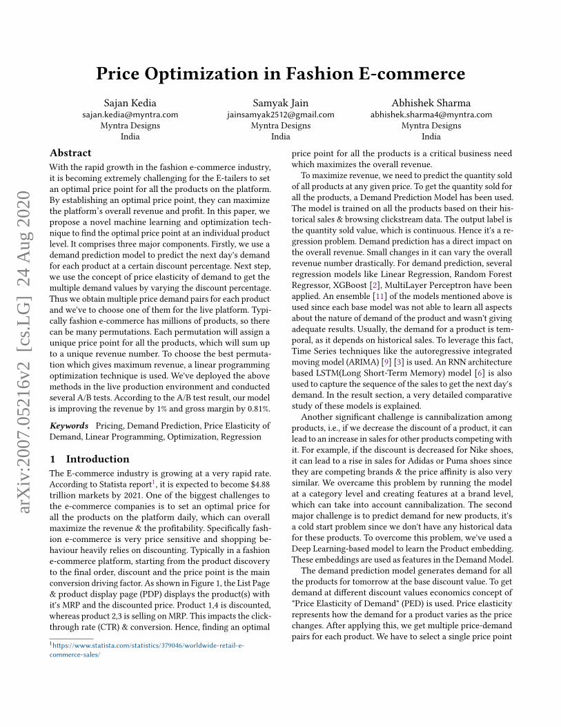
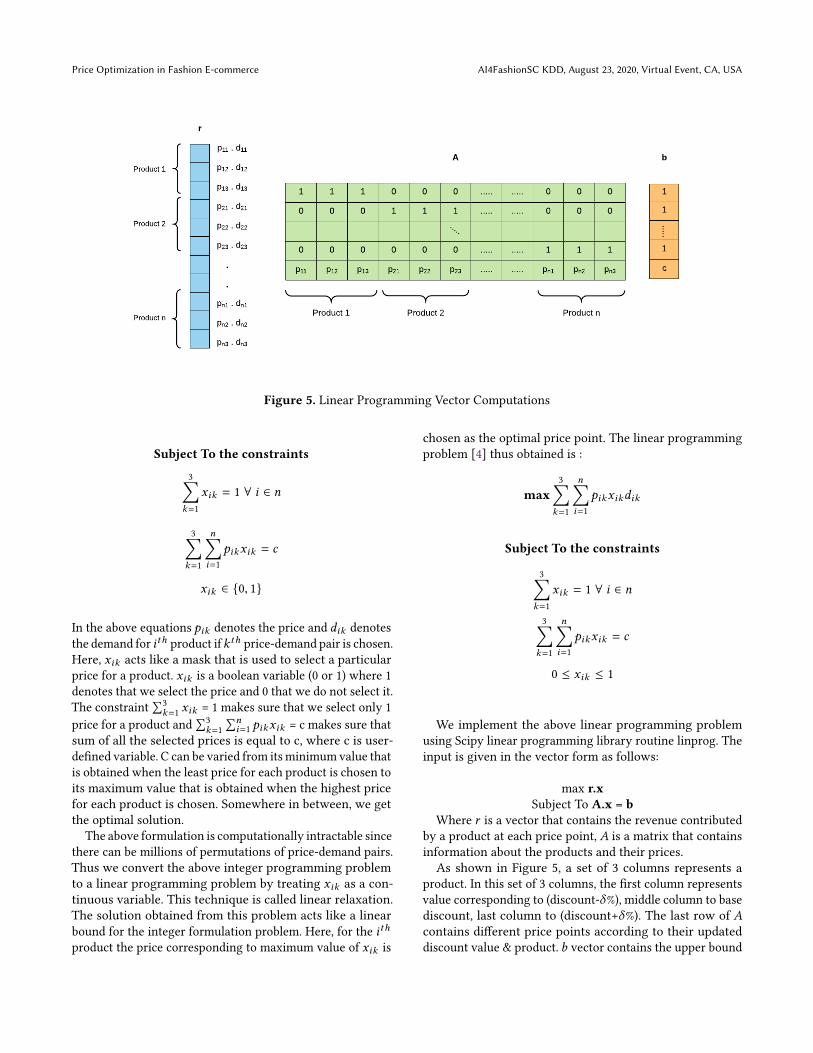
Figure 5. Linear Programming Vector Computations

Subject To the constraints

3∑k=1

xik = 1 ∀ i ∈ n

3∑k=1

n∑i=1

pikxik = c

xik ∈ {0, 1}

In the above equations pik denotes the price and dik denotesthe demand for ith product ifkth price-demand pair is chosen.Here, xik acts like a mask that is used to select a particularprice for a product. xik is a boolean variable (0 or 1) where 1denotes that we select the price and 0 that we do not select it.The constraint

∑3k=1 xik = 1 makes sure that we select only 1

price for a product and∑3

k=1∑n

i=1 pikxik = c makes sure thatsum of all the selected prices is equal to c, where c is user-defined variable. C can be varied from its minimum value thatis obtained when the least price for each product is chosen toits maximum value that is obtained when the highest pricefor each product is chosen. Somewhere in between, we getthe optimal solution.

The above formulation is computationally intractable sincethere can be millions of permutations of price-demand pairs.Thus we convert the above integer programming problemto a linear programming problem by treating xik as a con-tinuous variable. This technique is called linear relaxation.The solution obtained from this problem acts like a linearbound for the integer formulation problem. Here, for the ithproduct the price corresponding to maximum value of xik is

chosen as the optimal price point. The linear programmingproblem [4] thus obtained is :

max3∑

k=1

n∑i=1

pikxikdik

Subject To the constraints

3∑k=1

xik = 1 ∀ i ∈ n

3∑k=1

n∑i=1

pikxik = c

0 ≤ xik ≤ 1

We implement the above linear programming problemusing Scipy linear programming library routine linprog. Theinput is given in the vector form as follows:

max r.xSubject To A.x = b

Where r is a vector that contains the revenue contributedby a product at each price point, A is a matrix that containsinformation about the products and their prices.As shown in Figure 5, a set of 3 columns represents a

product. In this set of 3 columns, the first column representsvalue corresponding to (discount-δ%), middle column to basediscount, last column to (discount+δ%). The last row of Acontains different price points according to their updateddiscount value & product. b vector contains the upper bound


of the constraints. All entries in b are 1 except the last one,which is equal to c. Here 1 represents that only one price canbe selected for each product, and c indicates the summationcorresponding to the chosen prices.

4 Results & AnalysisIn this section, we have discussed the data sources used tocollect the data, followed by an analysis of the data and theinsights derived from it. Different kinds of evaluation metricsused to check the accuracy are also discussed along with thecomparative study of different models used.

4.1 Data SourcesData was collected from the following sources :

• Clickstream data: this contained all user activitysuch as clicks, carts, orders, etc.

• Product Catalog: this contained details of a productlike brand, color, price, and other attributes related tothe product.

• Price data: this contained the price and the quantitysold of a product at hour level granularity.

• Sort Rank: this contained search rank and the corre-sponding scores for all the live products on the plat-form.

4.2 Analysis of DataAccording to the analysis, 20% of the products generate 80%of the revenue. Hence, it is required to price these productsprecisely. This is the biggest challenge when it comes to de-mand prediction. Figure 6 shows the distribution of quantity

Figure 6. Distribution of Quantity Sold

sold for all the products on the platform. It is evident that aminority of products contribute towards the total revenue.Figure 7 shows the elasticity distribution of the products

on the platform. The y-axis of the graph depicts the densityrather than the actual count frequency of the elasticity value.As discussed in Section 3.3, the determination of elasticity isa difficult task. All kinds of elasticity are experienced, and

hence elasticity is calculated at a product level. It is evidentfrom the figure that the range of elasticity is from -5 to +5. -5indicates that if the price is dropped, then demand increasesdrastically, and +5 suggests that if the price is increased, thendemand also increases by a large margin. It can be observedthat most of the time, elasticity value is 0; this is so because80% of the quantity of the product sold is 0. Lastly, it can beconcluded that most of the product’s elasticity lies between-1 to +1. Hence, most of the products are relatively inelastic,but there are few products whose elasticity is very high andare at extreme ends, so it has to be calculated accurately.

Figure 7. Distribution of Elasticity

4.3 Evaluation MetricTo evaluate the demand prediction models, mean absoluteerror & root mean squared error is used as a metric. Theyboth tell us the idea of how much the predicted output isdeviating from the actual label. For this scenario, coefficientof determination i.e., R2 or adjusted R2, is not a good measureas it involves the mean of the actual label. Since 80% of thetime actual label is 0 mean cannot accommodate it, and henceR2 cannot judge the demand model's performance.

4.4 ResultsIn this section results of different models are discussed in ta-ble 1. Majorly three different classes of the model were testedand compared. They include regressors, LSTM, and ARIMA.mae and rmse were chosen as the evaluation metric to com-pare these models. The reason for this choice is discussed insection 4.3. All the models were trained on historical data ofthe past three months, comprising of over a million records.For the test data, the recent single day records were used.First, different kinds of regressors were used; out of all theregressors, XGBoost gave the best result. It is so because it’stough to establish a functional relationship between inputfeatures and output demand. As XGBoost does not need toestablish any functional relationship, it performed better.


Model mae rmseLinear Regression 0.207 0.732Random Forest Regressor 0.219 0.854XG Boost 0.195 0.847MLP Regressor 0.254 1.471Ensemble 0.192 0.774LSTM 0.221 0.912ARIMA 0.258 1.497

Table 1. Comparative performance of various models

However, all individual regressors were not able to captureall aspects of the data, so an ensemble of all the regressorsgave the ideal result. The ensemble takes advantage of allregressors and hence is chosen. Then, after regressors, LSTM& ARIMA were also tried, but it failed to give the desiredresult as due to multiple external factors in the business, thedemand data for the products did not exhibit sequential &temporal characteristics.

4.5 Experimental DesignIn this section, we describe live experiments that were per-formed on one of the largest fashion e-commerce platforms.The experiments were run on around two hundred thousandstyles spread across five days. To test the hypothesis thatmodel recommended prices are better than baseline prices,two user groups were created:

• Set-A (Control group) was shown the baseline prices• Set-B (Treatment group) was shown model recom-mended prices.

These sets were created using a random assignment fromthe set of live users. 50% of the total live users were assignedto Set A and the rest to Set B.Users in Control and Treatment groups were exposed to

the same product. But the products were priced differentlyaccording to the group they belong to. Both groups werecompared with respect to the overall platform revenue andgross margin. Revenue is already defined and explained insection 3, whereas gross margin can be defined as follows :

GrossMarдin = (Revenue − (buyinд cost))/RevenueIn general, the gross margin in our scenario is pure profit

bottom line.In table 2, the first three instances correspond to the busi-

ness unit - Men's Jeans and Streetwear, while the last 2 areof Women's Western wear and Eyewear respectively.

In the case of Men's Jeans and Streetwear, there is a steadyincrease in both revenue and gross margin of the wholeplatform. From this, it can be concluded that the model rec-ommended price gave positive results for this business unit.

Percentage increment in Revenue GM % UpliftTest 1 0.96% 0.99%Test 2 1.96% 0.95%Test 3 0.09% 0.49%Test 4 3.27% -0.41%Test 5 7.05% 0.15%

Table 2. A/B test results

In the case of Women's Western wear, there was a massivelift in revenue, but the gross margin fell. The reason for thisis that women's products were highly elastic. Small changesin price had a significant impact on demand. So due to themodel’s recommended price, there was a vast fluctuation indemand (i.e., demand for products increased), and the rev-enue thus increased. However, the gross margin was slightlyimpacted, and it decreased.

Eyewear is a small business unit, so the impact of discountchange is enormous, i.e., 7.05% increment in the revenue,whereas the GM increased by 0.15%.

Overall there was an approximately 1% increase in revenueof the platform and 0.81% uplift in gross margin due to modelrecommended prices. These are computed by taking theaverage of the first three instances since they belong to thesame business unit.

5 ConclusionFashion e-tailers currently find it extremely hard to decidean optimal price & discounting for all the products on a dailybasis, which can maximize the overall net revenue & theprofitability. To solve this, we have proposed a novel methodcomprising three major components. First, a demand predic-tion model is used to get an accurate estimate of tomorrow'sdemand. Then, the concept of price elasticity of demand isused to get the demand for a product at multiple price points.Finally, a linear programming optimization technique is usedto select one price point for each product, which maximizesthe overall revenue. Online A/B test experiments show thatby deploying the model revenue and gross margin increases.Right now, the prices are decided and updated daily, but inthe future, we would like to extend our work so that we canalso capture the intra-day signals in our model & accordinglydo the intra-day dynamic pricing.

References[1] M Babar, PHNguyen, V Cuk, and IG Kamphuis. 2015. The development

of demand elasticity model for demand response in the retail marketenvironment. In 2015 IEEE Eindhoven PowerTech. IEEE, 1–6.

[2] Tianqi Chen and Carlos Guestrin. 2016. Xgboost: A scalable treeboosting system. In Proceedings of the 22nd acm sigkdd internationalconference on knowledge discovery and data mining. ACM, 785–794.

[3] Javier Contreras, Rosario Espinola, Francisco J Nogales, and Antonio JConejo. 2003. ARIMA models to predict next-day electricity prices.IEEE transactions on power systems 18, 3 (2003), 1014–1020.


[4] MAH Dempster and JP Hutton. 1999. Pricing American stock optionsby linear programming. Mathematical Finance 9, 3 (1999), 229–254.

[5] Ralph E Gomory and William J Baumol. 1960. Integer programmingand pricing. Econometrica: Journal of the Econometric Society (1960),521–550.

[6] Klaus Greff, Rupesh K Srivastava, Jan Koutník, Bas R Steunebrink,and Jürgen Schmidhuber. 2016. LSTM: A search space odyssey. IEEEtransactions on neural networks and learning systems 28, 10 (2016),2222–2232.

[7] Rajan Gupta and Chaitanya Pathak. 2014. A Machine Learning Frame-work for Predicting Purchase by Online Customers based on DynamicPricing. In Complex Adaptive Systems.

[8] David Guthrie, Ben Allison, Wei Liu, Louise Guthrie, and Yorick Wilks.2006. A closer look at skip-gram modelling.. In LREC. 1222–1225.

[9] Maobin Li, Shouwen Ji, and Gang Liu. 2018. Forecasting of ChineseE-Commerce Sales: An Empirical Comparison of ARIMA, NonlinearAutoregressive Neural Network, and a Combined ARIMA-NARNNModel. Mathematical Problems in Engineering 2018 (2018).

[10] Lusajo MMinga, Yu-Qiang Feng, and Yi-Jun Li. 2003. Dynamic pricing:ecommerce-oriented price setting algorithm. In Proceedings of the 2003International Conference on Machine Learning and Cybernetics (IEEE

Cat. No. 03EX693), Vol. 2. IEEE, 893–898.[11] Xueheng Qiu, Le Zhang, Ye Ren, Ponnuthurai N Suganthan, and Gehan

Amaratunga. 2014. Ensemble deep learning for regression and time se-ries forecasting. In 2014 IEEE symposium on computational intelligencein ensemble learning (CIEL). IEEE, 1–6.

[12] Xin Rong. 2014. word2vec parameter learning explained. arXiv preprintarXiv:1411.2738 (2014).

[13] Rainer Schlosser and Martin Boissier. 2018. Dynamic pricing undercompetition on online marketplaces: A data-driven approach. In Pro-ceedings of the 24th ACM SIGKDD International Conference on Knowl-edge Discovery & Data Mining. ACM, 705–714.

[14] Vivek Kumar Singh and Kaushik Dutta. 2015. Dynamic Price Predictionfor Amazon Spot Instances. 2015 48th Hawaii International Conferenceon System Sciences (2015), 1513–1520.

[15] Daniel Solow. 2007. Linear and nonlinear programming. Wiley Ency-clopedia of Computer Science and Engineering (2007).

[16] Peng Ye, Julian Qian, Jieying Chen, Chen-hung Wu, Yitong Zhou,Spencer De Mars, Frank Yang, and Li Zhang. 2018. Customized Re-gression Model for Airbnb Dynamic Pricing. In Proceedings of the 24thACM SIGKDD International Conference on Knowledge Discovery & DataMining. ACM, 932–940.

price optimization in fashion e-commerce

Documents