J~urnul of Intrmutionaf .Cfone~~ and Finance ( 199 I ). 10. 3 10-329

Pricing foreign currency options under stochastic interest rates

KAUSHIK I. AMIN

School of Business Administration, The Unirersitjv of Michigan. Ann Arbor, MI 48109-1234. USA

AND

ROBERT A. JARROW

S.C. Johnson Graduate School of Management, Cornell University., Ithaca, NY 14853. USA

In this paper, we build a general framework to price contingent claims on foreign currencies using the Heath et al. (1987) model of the term structure. Closed form solutions are obtained for European options on currencies and currency futures assuming that the volatility functions determining the term structure are deterministic. As such, this paper provides an example of a bond price process (for both the domestic and foreign economies) consistent with Grabbe’s (1983) formulation of the same problem.

An American call (put) option on a foreign currency or currency futures gives the holder the right to buy (sell) a fixed amount of the foreign currency or currency futures, respectively, at a predetermined price at any time until a fixed expiration date. The corresponding European options can be exercised only at the expiration date. In the USA, listed call and put options on foreign currency and currency futures are traded on the Philadelphia Stock Exchange and the International Monetary Market at the Chicago Mercantile Exchange, respectively.

The existing academic literature studying the pricing of these options can be divided into two categories. In the first, both domestic and foreign interest rates are assumed to be constant whereas the spot exchange rate is assumed to be stochastic. Valuation models which assume constant interest rates are appealing due to their simplicity. Yet, these models trivialize the differences between futures prices and spot prices by ignoring the complications associated with marking to market; see Jarrow and Oldfield (1981). Empirical verification of this class of models has been disappointing (see Bodurtha and Courtadon, 1987; Goodman et al., 1985; Shastri and Tandon, 1986a, b; Tucker et al., 1988; Shastri and Wethyavivorn, 1987; and Melino and Turnbull, 1987, 1988).

The second class of models for pricing foreign currency options incorporate stochastic interest rates, and are based on Merton’s (1973) stochastic interest rate model for pricing equity options (see Feiger and Jacquillat 1979; Grabbe,

The authors gratefully acknowledge the helpful comments of IWO anonymous referees.

0261-5606~91/03~0310-20 c 1991 Butterworth-Heinemann Ltd

KAUSHWC I. AWN AND ROBERT A. JARROW 311

1983; and Adams and Wyatt, 1987). Unfortunately, this pricing approach does not integrate a full-fledged term structure model into the valuation framework. This is important since, in Merton’s (1973) formulation, every distinct exercise date for European calls requires a distinct bond (matching the maturity) to form the hedge. Hence, due to early exercise considerations, a continuum of distinct bonds are needed to value American type options. Without the entire term structure, Merton’s partial differential equation approach cannot be extended to price American claims. This consideration also applies to the pricing of foreign currency futures options, where marking to market again requires knowledge of the entire evolution of interest rates and a continuum of bonds.

This paper’s contribution is to provide an alternative class of option pricing models which incorporate stochastic interest rates yet avoid the shortcomings of Merton’s formulation. This approach is based on the martingale measure technique recently developed to price interest rate options; see Ho and Lee (1986) and Heath et ul. (1987). In particular, we apply the Heath et ul. (1987) model of the term structure to price foreign currency and currency futures options.

An outline for this paper is as follows. The next section introduces the terminology, notation, and assumptions underlying the economy. Section II describes the conditions necessary for an arbitrage-free economy. Section III applies the methodology to price European options on the spot exchange rate, while Section IV investigates forward and futures options. Section V explores the issue of domestic currency versus foreign currency valuation, and Section VI concludes the paper.

I. The economy

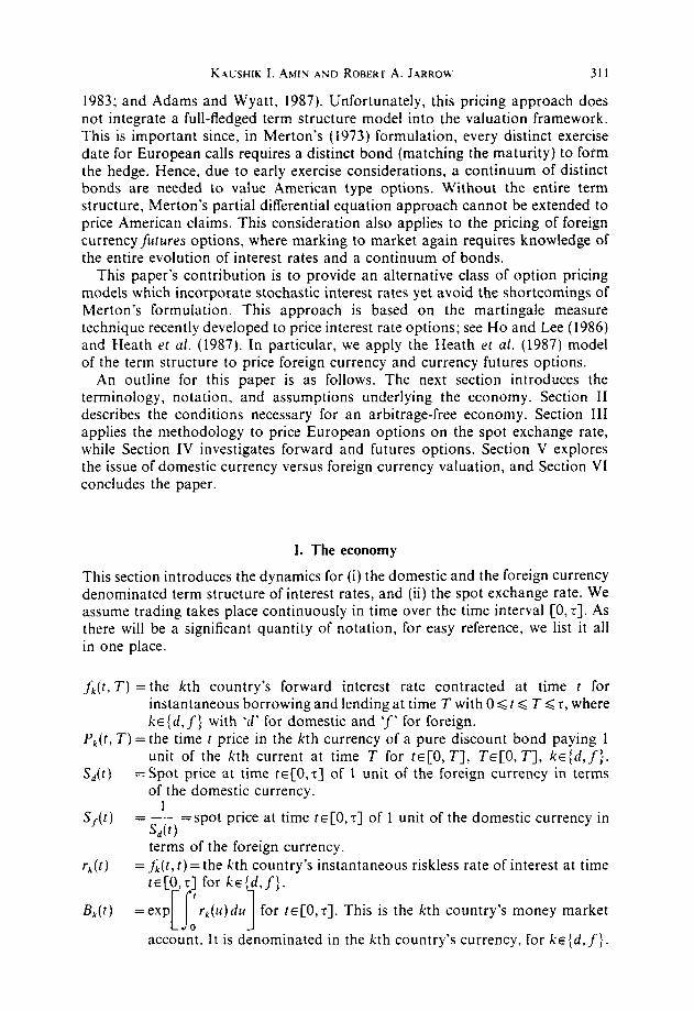
This section introduces the dynamics for (i) the domestic and the foreign currency denominated term structure of interest rates, and (ii) the spot exchange rate. We assume trading takes place continuously in time over the time interval [0, T]. As there will be a significant quantity of notation, for easy reference, we list it all in one place.

fk(t, T) = the kth country’s forward interest rate contracted at time t for instantaneous borrowing and lending at time T with 0 < t 6 T < T, where k~(n,f) with ‘d’ for domestic and ‘f’ for foreign.

Pk(t, T) = the time r price in the kth currency of a pure discount bond paying 1 unit of the kth current at time T for tE[O, T], TE[O, T], k~{d,f}.

S,(c) = Spot price at time t~[O,5] of 1 unit of the foreign currency in terms of the domestic currency.

1 S,(t) =-- =spot price at time re[O,s] of 1 unit of the domestic currency in

S,(t) terms of the foreign currency.

rk(t) = fk(t, t)= the kth country’s instantaneous riskless rate of interest at time te[O,r] for kg’d,f).

I

B,(r) = exp [S 1

T~(II)~CI for t~[O,s]. This is the kth country’s money market

accou,“t. It is denominated in the kth country’s currency, for k~(d,fj.

312 Priciny forriyn curwnc~ oplions

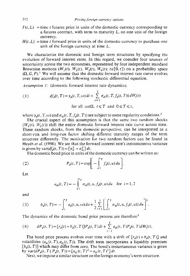
F(r, L) = time t futures price in units of the domestic currency corresponding to a futures contract, with term to maturity L, on one unit of the foreign currency.

H(t, L) = time t forward price in units of the domestic currency to purchase one unit of the foreign currency at time L.

We characterize the domestic and foreign term structures by specifying the evolution of forward interest rates. In this regard, we consider four sources of uncertainty across the two economies, represented by four independent standard Brownian motions (tVr(t), Wz(t), W3(t), W4(t); t~[O,s]) on a probability space (52, G, P).’ We will assume that the domestic forward interest rate curve evolves over time according to the following stochastic differential equation.

Assrrmpfion I: (domestic forward interest rate dynamics).

(1) df,(r, T)=z,(t, T,co)dt+ i adi(r7 T3 Sd(f, T)) dW(r) i= 1

for all CUE!& rd T and O<T<T,

where ~(t, T, w) and a,,,(~, T,f,(r, T)) are subject to some regularity conditions.’ The crucial aspect of this assumption is that the same two random shocks

(WI(r), Wz(r)) shift the entire domestic forward interest rate curve across time. These random shocks, from the domestic perspective, can be interpreted as a short-run and long-run factor shifting different maturity ranges of the term structure differently. The motivation for two random factors can be found in Heath et al. (1990). We see that the forward interest rate’s instantaneous variance is given by var(cif(r, T)) = [a:, + o~J dr.

The domestic bond price in units of the domestic currency can be written as:

(2)

Let

Pd(r, T)=exp[ -rld(r,n)dn]

and

a,,(r, T) = - s

T o,Jr, u,f,(r, 14) tlu for i= l,:!

f

s T

a,(r, u, o) du + i ,i [S

T

1 2

(3) b,(r, T) = - crJr, u, f;(r, u)) drr . I -I=1 t

The dynamics of the domestic bond price process are therefore3

(4) dP,(r, T)=[r,(r)+h,(r, T)]P,(r, T)dr+ i a,,(t, T)P,(r, T)dCy(t). i=l

The bond price process evolves over time with a drift of [r,,(r)+bd(r, T)] and volatilities (ad, (r, T), a,+(r, T)). The drift term incorporates a liquidity premium Cb,,(r, T)] which may differ from zero. The bond’s instantaneous variance is given by var(dP,(r, T)i’P,(r, T)) = [a,,(r, T)‘+a,:(r, T)‘] dr.

Next, we impose a similar structure on the foreign economy’s term structure.

KAUSHIK I. AMIN AND ROBERT A. JARROW

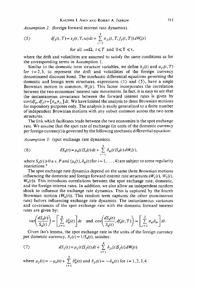
Assumption 2: (foreign forward interest rate dynamics)

313

i=2

for all osR, r<T and O<T <T,

where the drift and volatilities are assumed to satisfy the same conditions as for the corresponding terms in Assumption 1.

Similar to the domestic term structure variables, we define b,-(t) and aIi(t, T) for i=2,3, to represent the drift and volatilities of the foreign currency denominated discount bond. The stochastic differential equations governing, the domestic and foreign term structures, expressions (1) and (5), have a single Brownian motion in common, W2(r). This factor incorporates the correlation between the two economies’ interest rate movements. In fact, it is easy to see that the instantaneous covariance between the forward interest rates is given by

Ch?fd7 &,I = c o,,p,-J dt. We have limited the analysis to three Brownian motions for expository purposes only. The analysis is easily generalized to a finite number of independent Brownian motions with any subset common across the two term structures.

The link which facilitates trade between the two economies is the spot exchange rate. We assume that the spot rate of exchange (in units of the domestic currency per foreign currency) is governed by the following stochasticdifferential equation:

Assumption 3: (spot exchange rate dynamics).

(6) nsd(t)=~(d(f)Sd(f)dt+ i 6,i(r)S,(t)dWi(f), i=l

where s,(t) > 0 as. P and &(t), 6di(t) for i = 1, . . , 4) are subject to some regularity restrictions.4

The spot exchange rate dynamics depend on the same three Brownian motions influencing the domestic and foreign forward interest rate structures (kVr(t), W2(t), W3(t)). This introduces correlations between the spot exchange rate, domestic, and the foreign interest rates. In addition, we also allow an independent random shock to influence the exchange rate dynamics. This is captured by the fourth Brownian motion (W4(f)). This random term captures the other (non-interest rate) factors influencing exchange rate dynamics. The instantaneous variances and covariances of the spot exchange rate with the domestic forward interest rates are given by:

Given Ito’s lemma, the spot exchange rate in the units of the foreign currency per domestic currency, s,-(t) = l/s,(t), satisfies:

‘(7) dS~(t)=P~(f)S~(f)dt+ i bfi(c)Sf(f)dW(r)

i= I

where /c,(t)= -pLd(t)+ t 8zi(t) and 6,,(t)= -d,Jt) for i= 1,2,3,4. i=l

314 Priciny fivriyn currencj~ options

II. Arbitrage free international economy

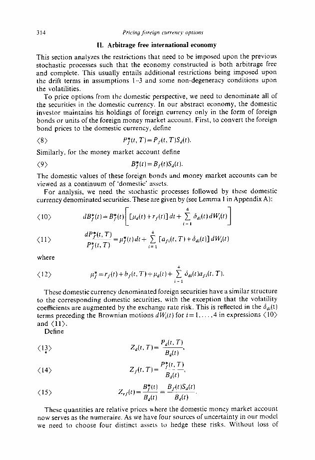
This section analyzes the restrictions that need to be imposed upon the previous stochastic processes such that the economy constructed is both arbitrage free and complete. This usually entails additional restrictions being imposed upon the drift terms in assumptions l-3 and some non-degeneracy conditions upon the volatilities.

To price options from the domestic perspective, we need to denominate all of the securities in the domestic currency. In our abstract economy, the domestic investor maintains his holdings of foreign currency only in the form of foreign bonds or units of the foreign money market account. First, to convert the foreign bond prices to the domestic currency, define

(8) p;(t, T)= P,(t, %CJ(t).

Similarly, for the money market account define

(9) B,*(t)= B,(0Xl(0.

The domestic values of these foreign bonds and money market accounts can be viewed as a continuum of ‘domestic’ assets.

For analysis, we need the stochastic processes followed by these domestic currency denominated securities. These are given by (see Lemma 1 in Appendix A):

(10) [~(d(t)+T/(f)] nt+ r 6,i(t)ciWi(t) i=l 1 (11) dpq;*;;y;; =/q(t) dt + t [Ufi(f, T) + s&(t)] dW,(t)

/ ’ i= 1

where

(12) 11; =r,(r)+b,(t, T)+/c,(r)+ i bdi(t)Uyi(t, T). i=l These domestic currency denominated foreign securities have a similar structure

to the corresponding domestic securities, with the exception that the volatility coefficients are augmented by the exchange rate risk. This is reflected in the ddi(t) terms preceding the Brownian motions nw,(t) for i= 1,. . ,4 in expressions ( 10) and (11).

Define

(1;)

(14)

(15)

P*(t, 7-J Z,(t, T) = -~

B,,(f) ’ P;(L T)

Z,(t, T) = ___ &t(t) ’

B;(r) Z,,(t)= __ =

BJW,(t)

b(t) W) ’ These quantities are relative prices where the domestic money market account

now serves as the numeraire. As we have four sources of uncertainty in our model we need to choose four distinct assets to hedge these risks. Without loss of

KALSHIK I. AWN AND ROBERT A. JARROU 315

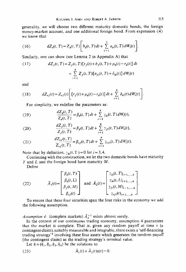
generality, we will choose two different maturity domestic bonds, the foreign money-market account, and one additional foreign bond. From expression (4) we know that

(16) dZ,(t, T) =Z,(t, T) [

bd(t, T) dr + ~ a,,(r, T)dWi(r) , i=l 1

Similarly, one can show (see Lemma 2 in Appendix A) that

(17) dZ,(r, T) =Z,(t, T)[:JO+ b,(t, T)+P,(~)--r,(t)] dr

+ i: Zf(r, T)Cafi(t, T) + Jdi(t)l dW(t)

i=l

and

(18) dZ,,(t) = Z,,(r) [

[q(t) +iG)- M)l &+ i a,,(t) dWi(r) . i=l 1

For simplicity, we redefine the parameters as:

(19)

cw

C-21)

“,“;~‘f,‘=/$(r, T)dr+ i Ydi(r, T)dW,(r), d 9 i=l

:;I”,:’ = j?/(r, T) dr + i ‘J/Jr, T) dw(r), / ’ i=l

i=l

Note that by definition, ydi(t,T )=0 for i= 3,4. Continuing with the construction, we let the two domestic bonds have maturity

T and L and the foreign bond have maturity M. Define

(22) A,(r)= [ t!(!;:] and A,(r)= [ ~~~~~~~~~.

. .

To ensure that these four securities span the four risks in the economy we add the following assumption.

Assumption 4: (complete markets) 1; 1 exists almost surely. In the context of our continuous trading economy, assumption 4 guarantees

that the market is complete. That is, given any random payoff at time T (a contingent claim), suitably measurable and integrable, there exists a ‘self-financing trading strategy’5 involving these four assets which generates the random payoff (the contingent claim) as the trading strategy’s terminal value.

Let 9 = (q,, qz, q3, v4) be the solutions to

(23) A,(r)+A2(r)fj(r)=0.

316 Pricing foreign currenc~v oprions

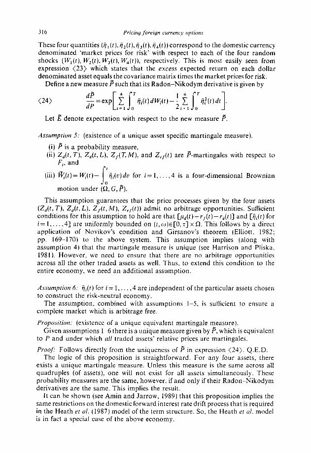
These four quantities (u,(t), rjJ(r), dj(r), da(t)) correspond to the domestic currency denominated ‘market prices for risk’ with respect to each of the four random shocks (WI(t), Wz(t), Wj(r), W4(t)), respectively. This is most easily seen from expression (23) which states that the c.~ccss expected return on each dollar denominated asset equals the covariance matrix times the market prices for risk.

Define a new measure P such that its Radon-Nikodym derivative is given by

(24) rli(r)d~i(r)-~ ,~ ’ -’ I I o Vi (r)dr s 1 .

Let i? denote expectation with respect to the new measure is.

Assumption 5: (existence of a unique asset specific martingale measure).

(i) P is a probability measure, (ii) Z,(t, T), Z,(t,L,), Z,(T,M), and Z,,(t) are P-martingales with respect to

F,, and

(iii) @i(t)= wi(t)- s

‘ili(” for i= 1,. . . ,4 is a four-dimensional Brownian

motion under (A, G, P).

This assumption guarantees that the price processes given by the four assets (Z,(t, T), Z,(t, L), Z,(t, M), Z,,-(r)) admit no arbitrage opportunities. Sufficient conditions for this assumption to hold are that [,u,Jt)+rJr)-‘Jr)] and [iji(r) for i= 1,. . . ,4] are uniformly bounded on (r,w)E[O, r] x R. This follows by a direct application of Novikov’s condition and Girsanov’s theorem (Elliott, 1982; pp. 169-170) to the above system. This assumption implies (along with assumption 4) that the martingale measure is unique (see Harrison and Pliska, 1981). However, we need to ensure that there are no arbitrage opportunities across all the other traded assets as well. Thus, to extend this condition to the entire economy, we need an additional assumption.

Asscrmprion 6: vi(t) for i= 1,. . . ,4 are independent of the particular assets chosen to construct the risk-neutral economy.

The assumption, combined with assumptions l-5, is sufficient to ensure a complete market which is arbitrage free.

Proposifion: (existence of a unique equivalent martingale measure). Given assumptions l-6 there is a unique measure given by P, which is equivalent

to P and under which all traded assets’ relative prices are martingales.

Proof Follows directly from the uniqueness of P in expression (24). Q.E.D. The logic of this proposition is straightforward. For any four assets, there

exists a unique martingale measure. Unless this measure is the same across all quadruples (of assets), one will not exist for all assets simultaneously. These probability measures are the same, however, if and only if their Radon-Nikodym derivatives are the same. This implies the result.

It can be shown (see Amin and Jarrow, 1989) that this proposition implies the same restrictions on the domestic forward interest rate drift process that is required in the Heath et al. (1987) model of the term structure. So, the Heath et al. model is in fact a special case of the above economy.

KAUSHIK I. AMIN AND ROBERT A. JARROW 317

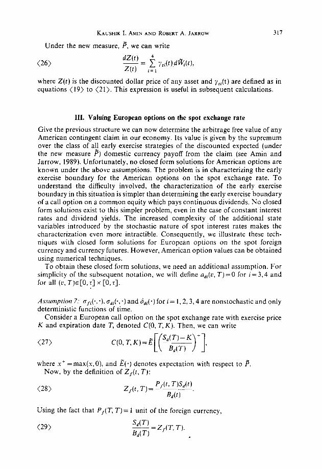
Under the new measure, P, we can write

(26) dZ(t) 4 z(t) = 1 ?;i(t)dR(r),

i=l

where Z(t) is the discounted dollar price of any asset and rri(t) are defined as in equations (19) to (21). This expression is useful in subsequent calculations.

III. Valuing European options on the spot exchange rate

Give the previous structure we can now determine the arbitrage free value of any American contingent claim in our economy. Its value is given by the supremum over the class of all early exercise strategies of the discounted expected (under the new measure P) domestic currency payoff from the claim (see Amin and Jarrow, 1989). Unfortunately, no closed form solutions for American options are known under the above assumptions. The problem is in characterizing the early exercise boundary for the American options on the spot exchange rate. To understand the difficulty involved, the characterization of the early exercise boundary in this situation is simpler than determining the early exercise boundary of a call option on a common equity which pays continuous dividends. No closed form solutions exist to this simpler problem, even in the case of constant interest rates and dividend yields. The increased complexity of the additional state variables introduced by the stochastic nature of spot interest rates makes the characterization even more intractible. Consequently, we illustrate these tech- niques with closed form solutions for European options on the spot foreign currency and currency futures. However, American option values can be obtained using numerical techniques.

To obtain these closed form solutions, we need an additional assumption. For simplicity of the subsequent notation, we will define adi(r, T) = 0 for i= 3,4 and for all (c, T)E[O, T] x [O,r].

Assumption 7: a~,(., *), ~di(., *) and 6,i( .) for i= 1,2,3,4 are nonstochastic and only deterministic functions of time.

Consider a European call option on the spot exchange rate with exercise price K and expiration date 7’, denoted C(0, T, K). Then, we can write

07) C(0, T,K)=e[(Sd;;;K)+],

where .Y+ =max(.u,O), and E(s) denotes expectation with respect to P. Now, by the definition of Z,(t, T):

(28) Z,(t, T) = P,k T)&(t)

Bd(f) .

Using the fact that P,-(T, T)= 1 unit of the foreign currency,

(29) S,(T) ~ =Z,-(T, T). B,(T)

318 Pricing jbrrign curwmy options

This implies that we can write

(30) K +

Z,(T,T)-- >I B,(T) ’

Substituting Lemmas 3 and 4 of Appendix A into equation (30) yields:

(31) C(O.T.K)=B[Z,(O,~)exp(~~~~~~u,.(~,T)CJ,i(c)]d~(r)

[U/i(L;, T) + S,,(C)]’ dV

)

- KP,(O, T)

U,i(U, T) d~i(V)- - C :if: JoT~:i(Cl~ T)dc)]‘.

Noting that Z,(O, T)= P,(O, T)S,(O) and using Lemma 5 in Appendix A, the above can be rewritten as

(32) C(O,7-, K) = P,(O, T&(O)@(h) - KP,(O, T)@(h - i),

where

and

(34) 1 [Ufi(L’, T)+6,i(c)-Udi(~., T)12 do.

A direct application of the second part of Lemma 5 in Appendix A now yields the price of the corresponding put option, denoted P(0, T, K), to be

(35) P(0, T, K) = KP,(O, T)@( -h + <) - P,(O, 7-)&(0)0(-h).

If we write out the expression for dF(t, T)/F(t, T) (where F(t, T) is the forward rate of exchange, i.e., S,(t)P,.(r, T)/P,(t, T)), the volatility term is exactly the term in brackets in equation (34). Hence, with this identification, expression (34) is a parameterized version of Grabbe’s (1983) formula. We see that the ‘volatility’ of the foreign currency option reflects not only the ‘volatility’ of the spot exchange rate, but also the ‘volatility’ of the domestic and foreign forward interest rates as well. The advantage of our framework, as distinct from that of Grabbe (1983), is that our model explicitly incorporates a continuum of traded domestic and foreign discount bonds into the analysis. This additional structure enables the pricing of foreign currency futures options, to which we now turn.

IV. Futures contracts, forward contracts and their options

In this section, we extend the previous analysis to the pricing of futures and forward contracts and European options on these contracts. The spot foreign

KAUSHIK I. AWN AND ROBERT A. JARROW 319

currency can be viewed as identical to a risky asset paying a stochastic dividend yield equal to the foreign currency spot interest rate. As it costs nothing to enter into a futures contract and the value of a futures contract is continuously reset to zero, by risk-neutrality, the futures price must be a P-martingale. We can use this observation to determine the futures price.

The futures price is given by the following expression (see Lemma 1 in Appendix B for the proof):

(36) F(t, T)=F(O, T)exp

[a/i(c, T)+ S,i(U)-adi(L., T)12 dv 1 9

where the time zero futures price is given by

(37) F(0, T) = P,(O, mf(O)

P,(O, 7-1

a,i(U, T)[Udi(L’, T)-Ufi(~, T)-~di(t’)] dc 1 .

It is well known that the forward price is given by the following expression:

(38) H(0, T) = P,(O, T)?,(O)

P,(O, T) ’

Combining this with expressions (36) and (37) gives the relationship between the futures and forward exchange rates:

U,i(c, T)[U,i(L., T)-U/i(L:, T)-6,,(()] dc 1 .

The forward and the futures prices differ only by the exponential term in the above expression which reflects the covariance between short rates and long-term bond prices. An interesting observation is that a deterministic domestic term structure is sufficient to make the domestic futures price equal to the forward price. This equivalence is independent of the foreign term structure volatilities. This fact can be explained by realizing that the spot currency can be viewed as a risky asset paying a stochastic dividend yield equal to the foreign spot interest rate. We know from Jarrow and Oldfield (1981) that a stochastic dividend yield is not what causes the difference between futures and forward prices.

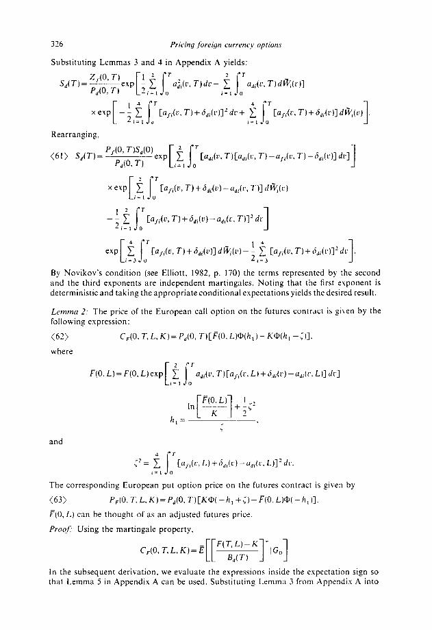
Similar to the case for the call option in Section III, we can use the martingale property to evaluate an expression for the price of a European futures option. The price of the European call option with maturity T and strike price K on the fitures contract with maturity L> T, denoted C,(O, T, L,K), is given by the following expression

(40) C#, T, L, K)=P,(O, T)CRO, L)@(h,)--K@(h, -;)I,

320

where

and

Pricing [breign currency options

F(0, L)= F(0, L)exp Ii~=, f f aa,(c, T)[afi(c,L)+ba,(v)-aadt',L)]dc 1,

hi=

(42)

where

~' = ,~1 [ayi(c, L) + 6ai(v) -- aai(c, L)] 2 dr.

The corresponding European put option price with maturity date T and strike price K on the futures contract with maturity L, denoted Pt.(O, 7", L, K), is given by

(41) Pr(O,T,L,K)=Pa(O,T)[KdO(-ht +(.)-F(O,L)O(-ht)].

We can think ofF(0, L) as an adjusted futures price where the adjustment depends on the volatility of the domestic and foreign term structures. The proofs of expressions (40) and (41) can be found in Lemma 2 in Appendix B.

Notice that the definition of ff is identical to that given in equation (34). Hence, the volatility term is exactly the same as in the case of the spot currency option. It corresponds to the volatility of the forward price. As the futures and the forward price differ only by a deterministic quantity, the volatility of the futures price is also identical.

The price of a European option with maturity date T and strike price K on a forward contract with maturity L, denoted C,(O,T,L,K), is given by the following expressions:

Ctt(O, 7", L, K)= Pa(O, r)[/4(0, L )aO(h2)- K q)(h,. -~)],

F±fo /7(0, L)= H(0, L)exp [a~i(t', T ) - a:i(v, L)] L i = l

× [ a f i ( v , L) + 3di(V) - - a d i ( l : , L)] dcJ,

is defined as expression (40) , and h 2 is given by

H L) 1 In + 2 ~-'

h2=

The corresponding put option price, denoted by Pn(O, T, L, K), is given by

(43) Pn(O, T, L, K)= Pd(O, T)[KO)(- h2 + ~)- /7(0, L ) ~ ( - h 2 )].

The proofs of these expressions are in Lemma 3 of Appendix B. These valuation formulas so obtained are testable, given estimation of the

volatilities given in assumptions 1-3. A comparison of the option on the spot

KACSHM I. AWN AND ROBERT A. JARROW 321

(expression (32)), the option on the futures (expression (40)). and the option on a forward (expression (42)) shows that all three values differ. If the option on both the forward and futures contract matures at time T (i.e., L= T). then the option on the spot and the option on the forward have identical values. Yet, the option on the futures has a different value. This difference emphasizes the importance of stochastic interest rates when valuing futures options. Indeed, if interest rates were deterministic, then all three values would be identical in the case where L= T.

V. Valuation under a foreign trader based perspective

The selection of the domestic currency versus the foreign currency was arbitrary in the preceding sections. Consequently, the analysis applies equally well to a foreign trader valuing claims in the foreign currency. The notation just needs to be symmetrically transformed. However, this observation leads to a subtle, but important insight.

When changing perspectives from a domestic trader with assets denominated in the domestic currency to a foreign trader with assets denominated in the foreign currency, the equivalent martingale measure of the proposition will change. This is true even if both traders have identical probability beliefs represented by P on (12, G). This follows because although Z(r) as given by expression (26) is a P-martingale, the foreign currency denominated relative price with the foreign money market account as the denominator need not be a p-martingale. To see this, consider Z,, which is a martingale under P. We have

Z,,(t) = B,WdO)

R,(t) ’ The analogous expression from the foreign trader’s perspective is

&f(r)&(r) KJ(t) 1

B,(t) UcP,(t) &-W

In general, if Z,, is a martingale, (l/Z,r) is not. Consider the stochastic differential def

equation6 governing the evolution of l/Z,,(t) = Z,*,(t):

dZ,; -----_=- Z$

i: ;‘,,$i@Jt)+ i i’pt. i=l i=l

The drift term in this expression is clearly non-zero, implying that l/Z,, is not a martingale.

This has an intuitive economic explanation as well. To make the argument in its simplest form, let both the domestic investor and the foreign investor be risk averse in assets denominated in their own currencies. Let the domestic investor have probability beliefs P and the foreign investor probability beliefs P. This is an acceptable system of beliefs. Under the domestic denominated money market relative price, the foreign trader appears risk neutral (because of the proposition). Yet, he is not. To consume. he must first move his assets into the foreign currency, and he is subject to exchange rate risk. The risk is real and he requires a positive market price of risk for bearing it. Hence, from his perspective, denominating

322 Priciny ftireign currmc~~ options

relative prices in foreign money market accounts, the analogous B from an analogous proposition will differ from his beliefs P. This completes the explanation.

From a practical perspective, once a particular currency is chosen as a base currency, option valuation can proceed as in Sections I-IV. There is no problem in currency option valuation. One can go from domestic prices to foreign prices at the spot exchange rate. The warning occurs when switching currency perspective including the denomination, i.e., the money market account. Then, to value options, one needs to change the risk neutral probability measure as well.

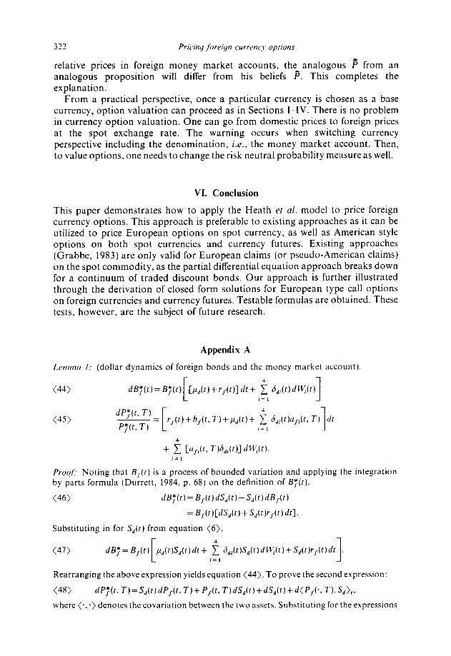
VI. Conclusion

This paper demonstrates how to apply the Heath ef al. model to price foreign currency options. This approach is preferable to existing approaches as it can be utilized to price European options on spot currency, as well as American style options on both spot currencies and currency futures. Existing approaches (Grabbe, 1983) are only valid for European claims (or pseudo-American claims) on the spot commodity, as the partial differential equation approach breaks down for a continuum of traded discount bonds. Our approach is further illustrated through the derivation of closed form solutions for European type call options on foreign currencies and currency futures. Testable formulas are obtained. These tests, however, are the subject of future research.

Appendix A

Lcwrwr 1; (dollar dynamics of foreign bonds and the money market account).

(44)

(45)

dB,*(f)=B;(t) [

[/~d(t)+rf(t)]df+ 2 ci,,(r)t/W,(t) i=l 1

dPf(r, T) 1

P;(t, T) ‘-,(t)+b/(t, T)+df)+ 1 S,Jf)~l/~(t, T) clt i=l 1

+ i [a&, T)6,,(t)] tin;(f). i=l

Proof Noting that B/(C) is a process of bounded variation and applying the integration by parts formula (Durrett, 1984, p. 68) on the definition of B;(t),

(46) tlB;(r)=B/(t)rlS,(r)+S,(r)ciB/(t)

=B/(t)[dS,(t)+S,(r)r/(f)dt].

Substituting in for S,(t) from equation (6),

(47) dB;=B,(r) [ ~Jt)SJt)dt+ i B,i(t)S,(r)rlCt~(t)+S,(t)r~(t)dt 1 i=l Rearranging the above expression yields equation (44). To prove the second expression:

(48) dP;(r, T)=S,(r)dP/(t, T)+ P,(t, T)dS,(t)+dS,(r)+d(P,(., T).S,>,,

where (*;) denotes the covariation between the two assets. Substituting for the expressions

KACSHIK I. AMIN AND ROBERT A. JARROW 3’3

and noting that

d(P/(‘, T),S,),= ~ ci,i(t)S,(f)a/i(f. T)P/(f, T)dt i=l yields the desired result. This completes the proof.

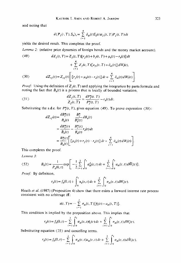
Lemnzn 2: (relative price dynamics of foreign bonds and the money market account),

(49) dZ,(t, V=Z,(t, T)[r,(t)+b,(t, T)+~d(~)-rd(r)ldr

+ i Z,(r, T)[a/j(f* r)+s,itf)] dkK(t), i=l (50) dZ,/(f)=Z,/(f) .[ C~~(f)+~~,(f)-r,(t)ldf+ i ci,i(f)dW,(f) i=l 1 Pro@? Using the definition of Z,-(t, T) and applying the integration by parts formula and noting the fact that BJt) is a process that is locally of bounded variation,

(51) dZ,(f, T) dPT(f. T) ------= Z,(f> T) P;(f, T)

-r,(t)dt.

Substituting the s.d.e. for P;(t, T), gives equation (49). To prove expression (50):

(q(f) dZ,,(f)= .-~ - Y

B‘,(f) ---c/B,(t) ES(f)

dB;(t) B;(t)

B,(f) ---rr,(t)df B,(f)

B;(t) = B(I, Mf)+r,(f)-rJt)]dt+ i Sd,(t)dM/(t) J i=l 1

This completes the proof.

Lenmn 3.

a;i(c.t)dc+ t s

I

(52) BJt) = u,,(~.f)di7vi(c)]. i=l 0 Proq/I By definition,

1

f rd(f)=AAO,f)+ r,(u,r)dr+ i 0 I I r7JL’, f) dWi(V). i=* 0

Heath et al. (1987) (Proposition 4) show that there exists a forward interest rate process consistent with no arbitrage iff:

i=l

This condition is implied by the proposition above. This implies that

r,(r)=f,(O.t)- t s

, cJdi(L’. f)lj,(I.)fil. + t

I odi(L.,f)dy(L.). i=l 0 s i=l 0

Substituting equation (15) and cancelling terms.

324

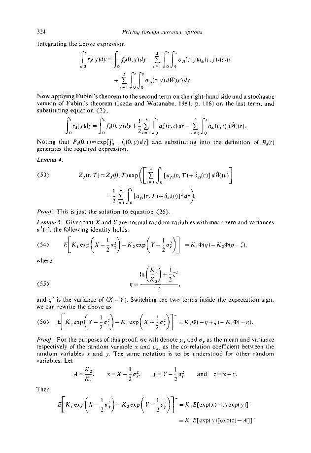
Integrating the

Pricity ./iwriqlrf crrrrrnc~~ opriotfs

above expression

, ss Y

a,,(r, 4’) tf Wi(L’) d_v. i=l 0 0

Now applying Fubini’s theorem to the second term on the right-hand side and a stochastic version of Fubini’s theorem (Ikeda and Watanabe, 1981, p. 116) on the last term, and substituting equation (2),

j+)d,.= j; /m):~~Y+ ;,$ , * j+wr-;, Ja,,li.r)dw.~.

Noting that P,(O, t) = exp[Ib -f,(O, y) dy] and substituting into the definition of B,(r) generates the required expression.

Letntm 4.

(53) Z,(t,T)=ZJ(O,T)exp ([ j

t ‘[nl-,(~.r)+6,,(r)]dit;(c) i=l II 1 -;,i j’[Uli(l.,T)+6di(C),zdl:).

L I 0

Proojl This is just the solution to equation (26).

Lmznw 5: Given that X and Y are normal random variables with mean zero and variances g2(*), the following identity holds:

(54) ~[~,exp(X-~~~)-K~exp(Y-14!1+=h.,m(il)-h.,m(n-;).

where

i

and c2 is the variance of (X- Y). Switching the two terms inside the expectation sign. we can rewrite the above as

Proof! For the purposes of this proof, we will denote /‘I- and 6, as the mean and variance respectively of the random variable .Y and px, as the correlation coefficient between the random variables I and y. The same notation is to be understood for other random variables. Let

and -_=s-y.

Then

= K, E[exp( y )[exp(:) - A]] -

KALSHIK I. AWN AND ROBERT A. JARROW 325

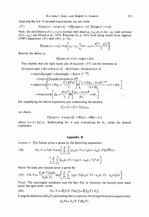
Applying the law of iterated expectations, we can write

(57) E[exp(s)-.l exp(y)]+ =E[[exp(-_)-A]‘E(exp(.r)I:=u)].

Now, the distribution of J/Z= II is normal with mean /~,+pJcr,,/~._)(u -pZ) and variance a_:(1 -p$) (see Mood et a!.. 1974, Theorem 16. p. 167). Now using results from Ingersol (1987) (equations (67) and (69), p. 14).

E[exp(J)I:=ri]=exp o’(1 -p’_)

~,+p,,O’(rl-/&)+~~ 0: 2 1 Rewrite the above as

E[exp( .r)I~=u]=exp(r+/?u).

This implies that the right hand side of equation (57) can be rewritten as:

E[exp(u)exp(r+pfc)lexp(u)2A]-E[A exp(r+/IItc)lexp(u)>A]

=exp(z)E[exp((l +B)u)lexp((l +P)rr)>A’ +8]

On simplifying the above expression and substituting the identity,

0; = 0; + C7f + 10,.6, pY_

we obtain

E[exp(x)-A exp(y)]’ =4)[~]-A@[~--a,].

where q=A + :af/a,. Substituting for A and multiplying by K, yields the desired expression.

Appendix B

Lrtmzn I: The futures price is given by the following expression:

(50 F(t,T)=F(O.T)exp [a&, r)+d,,(r)-n,,(c, r,] dngc)

l1 r

--ZT 1. [aJi(r3 T)+dfJ,(L.)-Udi(C, T)]*dl: ,

-,=I 0 1 where the time zero futures price is given by

(59) F(0, T)= p,a V,(O)

P,(O, T) adi(L.* T)[a,i(c, T)-a/i(r, r)-6,,(r)]dr 1

Proox The martingale condition and the fact that at maturity the futures price must equal the spot price, yields

(60) F(t,T)=~[F(T,T)IG,]=~[S,(T)IG,].

Using the definition of.S,( T) and noting that at maturity the foreign bond price equals unity

S,W=Z,tT, TPJT).

326 Pricing foreign currency options

Substituting Lemmas 3 and 4 in Appendix A yields:

s

r

adi(C, T)d~i(~)] i=L 0 T)+b,i(r)]‘dt,+ i jr ~a/i(~, T)+6,i(r)] d%(c)]. i=l 0

Rearranging,

(61) S,(T)= p$O;;)s,:o)exp [Udi(r’> T)[a,+i(r, T)-a,i(~, T)-~,;(c)] do] d 9 1

[a/i(L!, T)+6,i(r)-a,i(r, T)] dii/,(~)

[U/i(u, T)+Bdi(~‘.)-adi(l’, T)]‘dc 1 exp t

[ s T

[a/,(~, T)+bdi(u)] dtS/,(/1)- ; .$ [afi(u, T)+S,,(r)]‘dc 1=3 0 1 3 I

By Novikov’s condition (see Elliott, 1982, p. 170) the terms represented by the second and the third exponents are independent martingales. Noting that the first exponent is deterministic and taking the appropriate conditional expectations yields the desired result.

Lemnzn 2: The price of the European call option on the futures contract is given by the following expression:

where

F(0, L)=F(O, L)exp (Idi( T)[~/,(v, L)+d,,i(r)-~,i(r. L)] dr]

In

[ 1

+ ! -2 QO- L! K

i

h,= z . *

and

4 1 -2 _ 5 - 4 [u,~(L., L)+dd,(~)--~~,J~, L)]‘tk.

i=l 0

The corresponding European put option price on the futures contract is given by

(63) PF(O.T,L,K)=Pd(O,T)[K@(-h,++~(O,L)O(-h,)].

f(0, L) can be thought of as an adjusted futures price.

Proof! Using the martingale property,

In the subsequent derivation. we evaluate the expressions inside the expectation sign so that Lemma 5 in Appendix A can be used. Substituting Lemma 3 from Appendix A into

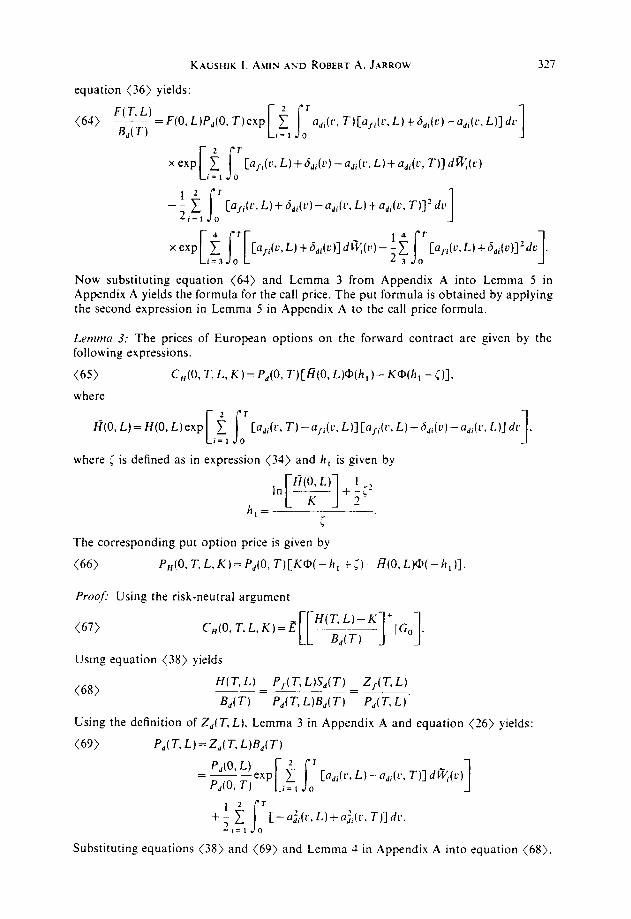
KAUSHIK I. ANN AND ROBERT A. JARROW

equation (36) yields:

327

(64) F(T, L) __ = f(O, L)P,(O, T)exp

B,(T) ‘Jdi(L.7 T)[a/i(r, L)+h,,(~‘)-_di(~., I_)] d[ 1

Cafi(c- L)+Bdi(L’)-UsJi(V, L)+U,,(c, T)]d*(r)

C’,,(‘,L)+d,i(c)-a,i(~. L)+u,,(~, T)]‘du 1 1 .

Now substituting equation (64) and Lemma 3 from Appendix A into Lemma 5 in Appendix A yields the formula for the call price. The put formula is obtained by applying the second expression in Lemma 5 in Appendix A to the call price formula.

Lenmn 3; The prices of European options on the forward contract are given by the following expressions.

(65) C,(O,T,L,K)=P,(O,T)[R(O,L)~(h,)-K~(h,-i)],

where

R(0, L)=H(O, L)exp [ s

t T

[adi(r> T)-a/i(~y L)][a/i(~, L)+~,~(L~)-Q,,(v, L)] dP 3 i=l 0 1

where ; is defined as in expression (34) and h, is given by

The corresponding put option price is given by

(66) P,(O, T. L, K ) = P,(O, T) [ K@( - h, + I, - f7(0, L)@( - h, ,]

Proof Using the risk-neutral argument

(67)

Using equation (38) yields

(68) Ht T, L) P/V, L&(T) Z/V-, L) c----_. BAT) PAT, L)B,(T) PAT. L)

Using the definition of Z,fT. L), Lemma 3 in Appendix A and equation (26) yields:

(69) PJT.L)=ZJT, L)B,(T)

CQ,i(t, L)-a,i(V, T)] dWi(r) 1 +‘i s

T

?,=I 0 C-aji(c, L)+ nf,(r+ T)] dc.

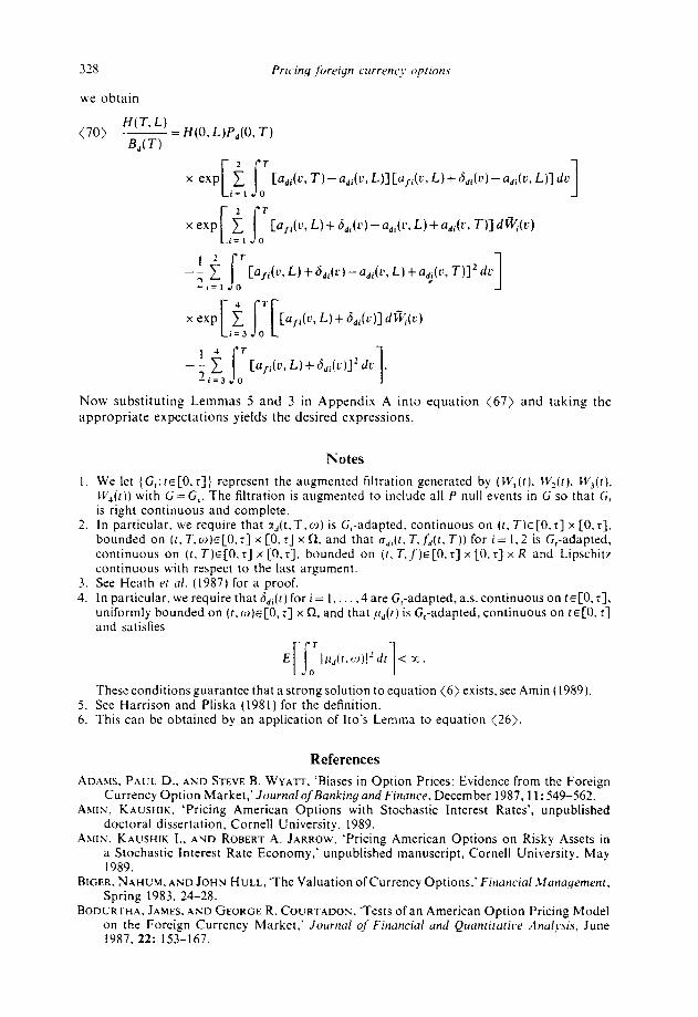
Substituting equations (38) and (69) and Lemma 1 in Appendix A into equation (68).

325

WC obtain

Pricing ftirriyn currenc~~ oprions

(70) H(T, L) ~ = H(0, L)P,(O, T) B,(T)

2 T

x fw C c s Cadi(cy T)-a,i(c, L)] [U,i(c, L)+ dd<(L’)-adi(U, L)] dc i=l 0 1

xexp t c s

T

Cafi(u. L)+ ddi(L’)-~di(L., L)+o,~(L’, T)] d%(c) i=l 0

C’fi(u* L)+a,i(c)-U,i(U, L)+Udj(ti, T)12 dti 1 [a/,(~, L)+h,Jc)] d%(c)

Ca/i(~.L)+d,,(~)12 dc 1 Now substituting Lemmas 5 and 3 in Appendix A into equation (67) and taking the appropriate expectations yields the desired expressions.

I.

2.

3

4:

5. 6.

We let (G,: t~[0, r]; represent the augmented filtration generated by (W,(t), W,(t). W3(r), B;(r)) with G=G,. The filtration is augmented to include all P null events in G so that G,

Notes

is right continuous and complete. In particular. we require that z,(t.T.w) is G,-adapted. continuous on (t. T)E[O. T] x [O.T]. bounded on (t, T,w)E[O,T] x [O,T] x0. and that cdi(r. T,I,(t, T)) for i= I.2 is G,-adapted, continuous on (t. T)c[O, r] x [0, T], bounded on (r. T.f)s[O. T] x [O. r] x R and Lipschitz continuous with respect to the last argument. See Heath er al. (1957) for a proof. In particular, we require that d,,(r) for i= I. (4 are G,-adapted, a.s. continuous on rc[O. r], uniformly bounded on (r,w)E[O, T] x R, and that p,,(r) is G,-adapted, continuous on rs[O. T] and satisfies

7 E

[s l&,(t.cJ)l’dr < %.

0 1

These conditions guarantee that a strong solution to equation (6) exists, see Amin (1989). See Harrison and Pliska (1981) for the definition. This can be obtained by an application of Ito’s Lemma to equation (26).

References

ADASIS, PAUL D.. AND STEVE B. WYATT. ‘Biases in Option Prices: Evidence from the Foreign Currency Option Market,‘JournalofBan&ny and Finunce. December 1987,11:549-562.

A~IIN, KAUSHIK. ‘Pricing American Options with Stochastic Interest Rates’, unpublished doctoral dissertation, Cornell University. 1989.

Axus, KAUSHIK I., AND ROBERT A. JARROW. ‘Pricing American Options on Risky Assets in a Stochastic Interest Rate Economy,’ unpublished manuscript, Cornell University, May 1989.

BIGER, NAHUXI, AND JOHN HULL, ‘The Valuation of Currency Options.’ Financial Management, Spring 1983. 24-28.

BODURTHA, JA~IES, AND GEORGE R. COURTADOS. ‘Tests of an American Option Pricing Model on the Foreign Currency Market,’ Journal of Finuncial und Quanrirurice Analysis, June 1987. 22: 1.53-167.

KAUSHIK I. AWIN AND ROBERT A. JARROW 329

Cox, JOHN, AND STEPHEN Ross. ‘The Valuation of Options for Alternative Stochastic Processes,’ Journal of Financial Economics, January 1976. 3: 145-166.

DURRETT, RICHARD, Browniun Motion and Martinyules in Ancllysis. California: Wadsworth. 1984.

ELLIOTT, ROBERT J., Stochastic Calculus and Applicafions, Berlin: Springer-Verlag. 1982. FEIGER, GEORGE, AND BERTRAND JACQUILLAT, ‘Currency Option Bonds, Puts and Calls on

Spot Exchange and the Hedging of Contingent Foreign Earnings,’ Journa! of Finance. December 1979. 5: 1129-l 139.

GARMAN, MARK, AND STEVEN KOHLHAGEN, ‘Foreign Currency Exchange Values.’ Journal of Inrernational Money nnd Finance. December 1983, 2: 231-237.

GOODMAN, LAURIE S., SUSAN Ross, AND FREDERICK SCHMIDT, ‘Are Foreign Currency Options Overvalued? The Early Experience of the Philadelphia Stock Exchange,’ The Journal of Futures Markets, Fall 1985, 5: 349-359.

GRABBE, J. ORLIN, ‘The Pricing of Call and Put Options on Foreign Exchange,’ Journal of International Money and Finance, December 1983, 2: 239-253.

HARRISON, J. M., AND S. R. PLISKA, ‘Martingales and Stochastic Integrals in the Theory of Continuous Trading,’ Stochustic Processes and Their Applicntions, July 198 1.11: 2 15-260.

HEATH, DAVID, ROBERT JARROW, AND ANDREW MORTON, ‘Bond Pricing and the Term Structure of Interest Rates: A New Methodology for Contingent Claims Valuation,’ unpublished manuscript, Cornell University, October 1987.

HEATH, DAVID, ROBERT JARROW, AND .ANDREW MORTON, ‘Contingent Claim Valuation with a Random Evolution of Interest Rates,’ The Recieu,of Futures Markers, forthcoming 1990.

Ho. T., AND S. LEE, ‘Term Structure Movements and Pricing Interest Rate Contingent Claims,’ Journal of Finance, December 1986. 41: 101 l-1028.

IKEDA, N., AND S. WATANABE, Stochusric Differential Equations und Di@ion Processes, New York: North-Holland, 1981.

INGERSOLL, JONATHAN E.. Theory of Financial Decision Mnking, Rowman and Littlefield, 1987. JARROW, ROBERT, AND G. OLDFIELD, ‘Forward Contracts and Futures Contracts,’ Journal of

Financial Economics, December 1981, 9: 373-382. MELINO, ANGELO, AND STUART M. TURNBULL, ‘The Pricing of Foreign Currency Options,’

unpublished manuscript, University of Toronto, December 1987. MELINO, ANGELO, AND STUART M. TURNBULL, ‘Pricing Foreign Currency Options with

Stochastic Volatility,’ unpublished manuscript, University of Toronto, June 1988. MERTON, ROBERT C., ‘The Theory of Rational Option Pricing,’ Bell Jortrnal of Economics and

Management Science, Spring 1973, 4: 141-183. Moor, ALEXANDER M., FRANKLIN A. GRAYBILL, AND DUANE C. BOES, Introduction to the

Theory of Stafisrics, New York: McGraw-Hill, 1974. SHASTRI, KULDEEP, AND KISHORE TANDON, ‘On the Use of European Models to Price American

Options on Foreign Currency,‘Journal of Futures ,lfarkets, Spring 1986.6: 93-108 ( 1986a). SHASTRI, KULDEEP, AND KISHORE TANDON, ‘Valuation of Foreign Currency Options: Some

Empirical Tests,’ Journal of Financial and Quantiratice Analysis, June 1986, 21: 145-160 (1986b).

SHASTRI, KULDEEP, AND KULPATRA WETHYAVIVORN, ‘The Valuation of Currency Options for Alternate Stochastic Processes,’ The Journal of Financial Research, Summer 1987, 10: 283-293.

TUCKER, ALAN L., DAVID R. PETERSON, AND ELTOS SCOTT, ‘Tests of the Black-Scholes and Constant Elasticity of Variance Currency Call Option Valuation Models,’ The Journal q/ Financial Research, Fall 1988. 11: 201-213.