Pricing in the London Market

Working Party

D.Sanders (Chairman) P.Grealy A.Hitchcox

T. Magnusson R.Manjrekar

J.Ross S.Shepley L.Waters

103

Insurance Convention1995 General

Pricing in the London Marke

5.

1. 2. 3.

Introduction Summary of the Paper Pricing Techniques used in practice 3.1

3.2

3.3 3.4 3.5 3.6 3.7 3.8

-Risk Excess of Loss Treaties Experience Rating Curve Fitting Exposure Rating Catastrophe Excess of Loss Aggregate based Methods Loss Based Methods Simulation/modelling type Methods Burning Cost Rating Exposure Rating Proportional Treaties Use of simulation methods Stop Loss treaties Credibility Theory Distribution Calculus Generalised Interactive Linear Models

4. Strategic Pricing 4.1 Introduction 4.2 Underwriting Targets & Control Cycle 4.3 Risk and Reward 4.4 Profit Testing 4.5 Underwriting Management Actuaries as Underwriters

Bibliography and Assorted Reading Appendix 1 Future Developments

1.1 Introduction 1.2 Neural Networks 1.3 Chaos Theory and New Distributions 1.4 Modelling Extreme Events 1.5 Relativistic Methods - Options and Curves 1.6 Financial Models

Appendix 2 Output from Catstrophe Simulation Appendix 3 Philbrick Tables

104

Pricing in the London Market

1. Introduction

1.1 The role of actuaries in pricing products in the London Market is an area where there

is considerable interest, both from the view of the actuary and from the view of

management. In the past underwriters have used their skills to identify risks that are

acceptable and quote rates that, in broad terms, have provided the shareholders or

names at Lloyd’s with acceptable profits. The number of cases of imprudent

underwriting is limited, although their consequences have often been disastrous. What

new features and ideas can an actuary bring to the pricing table to ensure that his skills

are valued and seen essential to all parties in the prudent management of the

business?

1.2 One of the main problems in writing this paper was trying to find the audience to focus

our comments. Clearly actuaries themselves would be in that audience, as would

Underwriters, Chief Executives, Finance Directors, Claims Managers, and even

trainees. The main conclusion was that the paper, although addressed for an Actuarial

Conference, should focus on the Management Team of a London Market operation.

The reasons for this will become apparent. Actuaries learning about this subject will

benefit from the additional reading and sophisticated software identified in Appendices.

What the Management Team needs to address is to view the actuarial role beyond the

annual reserving and fully involve him in the day to day management of the operation.

The role of the Actuary in Life Insurance is defined as the Financial Management of

the Insurance Operation. The President of the Institute, in his presidential address

endorsed the expansion of this role into General Insurance. This paper helps form a

basis of how this objective may be achieved.

1.3 We need to identify the reasons why an actuary should be involved in pricing. We

need to identify what skills set he can bring to the process that can be of benefit to

both the underwriter and his managers. The role needs both clarificationand

professional guidance to avoid such problems.

105

The reasons identified were as follows:-

1. Actuaries are trained in Financial Management and see the broader picture. An

actuary can identify assumptions in the underwriting process in an explicit form, for

example, claims inflation, investment income and so on. These may often be identified

only implicitly in an underwriter’s rate.

2. Actuaries can interpret the numbers in ways that may bring new insight into the risk.

3. Actuaries can act as a peer review to the individual risks, an aggregate pool of risks

and ultimately the whole book. The actuary can back up what may appear to be

difficult decision for the underwriter to take, and maybe form a focus for discussion of

particular problems as the relationship develops.

4. There is a clear relationship between pricing and reserving. An actuary involved in

pricing will be able to assist the reserving actuary in identifying particular features of

the account which are relevant in assessing the reserves.

5. The actuary gives a degree of comfort to the Board and shareholders, The actuary

is professional in his approach, and this should outweigh any vested interest that may

arise.

14 Given these attributes, there are clear problems which we have identified which will

lead to potential problems,

1. Actuarial resources are scarce, and there are a limited number of individuals with

the practical experience to undertake such a responsible task,

2. There is a need for clear communication and possible avoidance of jargon in

discussions between actuary and underwriter. Lack of clear communication could lead

to potential problems due to the lack of real understanding by the underwriter of the

consequences of not moving the rates

3. The involvement of actuaries in pricing needs full backing from the Chief Executive

downwards. Without this backing the task becomes impossible as other issues take

over. An example is the renewal of a risk not on price but because the underwriter has

led the risk for 10 years.

4. The actuary is often seen as giving post event justification to the underwriter. There

is often a short time between viewing the risk and acceptance, and the actuary may find

the assessment very difficult in the very limited time he has to analyse the risk.

106

1.5 In practice the role of the actuary in pricing in the London Market depends much on

the quality and quantity of information involved. There are clearly those risks were the

volume of information available will enable a reasonable price to be assessed by both

actuary and underwriter. It is the underwriters responsibility to write that risk, and in

doing so he may adjust the actuarial rate to take account of special features which have

been identified but which are difficult to price with any degree of certainty, for example

good risk management or a potential health hazard. The risks of lower information

quality may be pooled in some form as assessment, and eventually the whole book may

be reviewed as a valuation process. In a simplistic world, an actuary may identify, for a

given corporate profit objective, that the underwriter needs to write a specific book of

business to achieve a specific income. Let us say the actuarial income is £10 million. If

the underwriter writes those risks for £9.5 million, then the Board is aware, based on

the estimates, there is likely to be a deficit of £0.5 million on the results. Actual

experience may differ, but there is an early warning. Conversely if the underwriter

achieves £10.5 million in premium, then the Board can rest a little easier. To achieve

this level of understanding by all parties often needs input of an actuary The comfort

it may give to management is potentially enormous.

1.6 The London Market itself is a complex animal with conflicts between various risk

takers. Although the insurance product is for one year, the market in general views

continuity as important. This is indeed recognised in the long term planning and

objectives of both insurance companies and Lloyd’s. How often has the argument “We

have held the risk for twenty years” been used in the past to justify accepting a risk,

despite the fact the current rates may not support the risk. There is therefore a conflict

between short term pricing and long term pricing. This conflict helps generate the

variations we see in the rates, and managers clearly need to understand the potential

costs to the balance sheet, be it a syndicate or a company, and be able to maximise

profits within the risk constraints.

107

2. Summary of Paper

2.1 The paper is split into 2 primary sections, The purpose of these sections is to give a

good but broad view of the techniques. Examples are included in each of the sections

and are augmented by further examples in Appendix 3. A summary bibliography us

included together with references to additional reading. It should be noted that this

reference list is not comprehensive.

2.2 Section 3 of this paper deals with the individual risk methods which are used currently

in the day to day assessment of risks. Methods in this section are of value to those

actively assisting the underwriter.

Section 4 deals with the other issues which are normally implicit in the current pricing

but need to be expressed explicitly. These include risk/reward approaches and detailed

analysis of the cash flows and investment income (profit testing). These more general

approaches have been used, and possibly of more substantial benefit to management

than the “premium checking” approach in section 3. The concept of the insurance cycle

is introduced.

In Section 5 the challenging issue of actuaries being actively used in underwriting is

broached There are many views on this subject, and some of the issues are addressed

in that section.

In Appendix 1 we try to identify other methods which have been used by one or two

individuals to assess rates, but are generally not well known or adequately tested.

These include approaches from Financial Theory and from Neural Networks These

methods are rapidly becoming part of today’s actuary’s toolbox and is an area of

continual interest. These are both new directions and esoteric methods. Such methods,

if they pass the test, will become the standard pricing techniques of tomorrow.

108

3. PRICING TECHNIQUES USED IN PRACTICE

This section represents a simple “tool box” of techniques used in practice. It deals with

the loss cost only, i.e. does not consider expense and profit loadings. The structure of

the section is as follows:-

A list of the various pricing techniques available is given.

For each technique we try to provide the following:

Introductory remarks describe how it is used

The basic recipe is described.

Fuller details together with an illustrative example is given

References to further reading which contain more detail are provided.

Comments are made on application of the technique in practice,

The list of headings is as follows:

3.1 Risk excess of loss treaties

3.1.1. Experience rating

3.1.2 Curve fitting (including Pareto rating)

3.1.3 Exposure rating

3.2 Catastrophe excess of loss treaties

3.2.1 Aggregate-based methods

3.2.2 Loss-based methods

3.2.3 Simulation/modelling type methods

3.2.4 Burning Cost Bates

3.2.5 Exposure Bates

3.3. Proportional treaties

3.4. Use of simulation methods

3.5. Stop-loss treaties

3.6 Credibilitv Theory

3.7 Distribution Calculus

3.8 Generalised Interactive Linear Models

In addition to these see chapter 6 of The Foundations of Casualty Actuarial Science

which has many excellent worked examples.

109

3.1. Risk excess of loss treaties (Risk X/L)

3.1.1 Experience rating

(i) Introductory remarks

Experience rating (or burning cost) is an intuitively appealing approach to pricing,

taking into account as it does the cedant’s past loss history in trying to estimate future

losses to a layer. In theory it can be used for any class of business where there is an

adequate loss history, but it is perhaps most often used to price commercial fire, the

non-liability element of motor and liability business. It is also frequently used to price

medical malpractice business.

(ii) Basic recipe

The following is an example of how a layer might be priced using experience rating.

The FGU (fill ground up) development of the cedant’s large claims for a number of

past years of account is obtained. “Large” claims would typically mean claims which

do, or are likely to, impact the layer to be priced; the reinsurer’s reporting requirement

might typically be for all losses with an incurred equal to 50-75% of the deductible

after allowing for any indexation clause. (Note: in the US, development may not be

available by individual claims, only on an aggregate basis). The development is

adjusted for an appropriate measure of claims inflation to the period to be covered and

for any changes to, for example, policy wordings, business profile, claim size and

frequency, in market jargon it is reworked on an “as if” basis.

The ultimate for each loss in each year is then estimated using appropriate methods, for

example, a traditional triangulation method might be used, with tail factors and market

statistics applied where the development available is inadequate. Having adjusted the

loss development for IBNR, it can be put to the layer to be priced to produce an

estimate of the ultimate losses to the layer for each year under consideration.

Next, the premium in each year of account is [projected to ultimate and] inflated to the

period of cover allowing for any changes in coverage, past rate inadequacy,

appropriate sum insured inflation, etc. The estimated ultimate loss ratio, or perhaps

more frequently the burning cost (equal to the loss cost to the layer, the burn, divided

by the original cedant’s premium) to the layer for each year can then be calculated, a

110

suitable average selected, and loadings added for the reinsurer’s expenses, to get to the

indicated rate, per unit of direct premium written.

(iii) Illustrative example

Risk Excess of Loss

Casualty Burning Cost Rating Example

250,000 XS 250,000

Allocated Loss Adjustment Expenses Covered Pro Rata pro Loss

1. For each accident year, adjust each loss on as “as if” basis, for both indemnity

and expenses, for an appropriate measure of claims inflation, to the period to be

covered. For example consider 1991 accident year, 4 years after the start of the

accident year

Reported Reported Inflation Adjusted Adjusted Indemnity

Loss Expenses Factor Indemnity Expenses Expenses

(1) (2) (3) (4) (5) (6)

1 500,000 50,000 1.464 732,050 73,205 605,255

2 450,000 45,000 1.464 658,645 65,085 724.730 3 325,000 24,000 1.464 475,833 35,136 510.971

4 300,000 7,000 1.464 439,230 10,249 449,479

5 240,000 11,000 1.464 351,364 16,105 367,489

Total 1,815,000 137,000 2,657,342 200,582 2,857,923

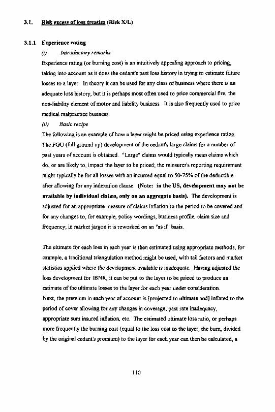
Use an appropriate method to estimate loss development factors to ultimate, hence to

estimate the ultimate value of each loss from 1. above, for each accident year under

consideration. For example by using a triangulation of the adjusted losses from 1:

111

Indemnitvy

Accident Development Year

Year 3 4 5 6 7 1988 2,277,920 2,961,295 3,656,565 4,764,620 5,980,775

1989 1.793,420 2,510,790 3,422,050 3,969,755

1990 1,568,855 2,353,285 3,136,930

1991 1,754,203 2,857,923

1992 3,855,907

3. For each accident year under consideration, increase the adjusted losses in 1. by the

appropriate factor to ultimate, and then put each loss to the layer to be priced to

calculate the loss in the layer For example the 1991 accident year

Adjusted Adjusted Develop Est UIt Est UIt indemnity Pro-rata Total

Loss Indemnity Expenses Factor Indemnity Expenses in Layer Expenses in Leyer

(7) (8) (8) (10) (10) (11) (12) (13) 1 732,050 73,205 2.449 1,793,074 179,307 250,000 25,000 275,000

2 658,645 65,885 2.449 1,613,767 161,377 250,000 25,000 275,000

3 475,833 35,138 2.449 1,165,498 86,068 250,000 18,462 268,462

4 439,230 10.249 2.449 1,075,844 25,103 250,000 5,833 255,833

5 351.384 16,105 2.449 860,676 39,448 250,000 11,456 281,458 2,657342 200,582 6,508,859 491,302 1,250,000 85,753 1,335,753

112

7:Ult

LOSS

1.200 1.225 1.250 1.333 1.500 Selected

1.250 1.200 1.333 1.457 Average

1992

1.629 1991

1.333 1.500 1990

1.160 1.363 1.400 1989

1.250 1.240 1.303 1.300 1988

6:7 5:6 4:5 3:4 Year

Factors Development

Accident

1.200 1.470 1.838 2.449 3.674 Cumulative

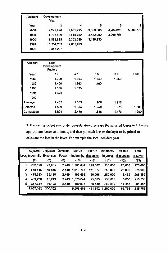
4. Adjust subject premiums to current premium levels, for example, for changes in rate

adequacy and changes in exposure and calculate exposure premium.

Accident

Year

1988

1989

1990

1991

1992

Adjusted Adjusted Indicated

Subject Losses Loss

Premium in Layer Rate

(14) (15) (16)

10,000,000 2,657,892 0.266

12,000,000 3,125,000 0.260

14,500,000 4,125,036 0.284

17,000,000 1,335,753 0.079

19,000,000 2,501,420 0.132

72,500,000 13,745,101 0.204

(17) Indicated loss rate

(18) Reinsurer loading (say)

(19) Exposure premium per unit of cedant’s direct premium

(iv) Practical considerations

In theory experience rating requires a statistically significant historical loss

development to be available for the cedant, and as such is much more suited to

working layers of an X/L programme. In practice there can be other sources of loss

development, for example IS0 development factors in the US, so full cedant FGU data

might not be needed. IS0 does a lot of work on development factors within layers

(see Pinto & Gogol), and when pricing US X/L it may not be necessary to work with

fu11 FGU losses, but simply to work with losses to the layer. Consideration must be

given to losses below the deductible; and how IS0 and similar development factors

cope with the losses, which incurred below the deductible, which might impact the

layer in the future’

Loss adjustment expenses must be allowed for appropriately depending on whether

they are included with the loss to be put to the layer, or are allocated on a pro-rata

basis.

113

0.224

100/80

0.255

3.1.2 Curve fitting 1

(i) Introductory remarks

A method which is not dissimilar to experience rating, but instead of using the FGU

data directly, a curve, of ten a Pareto, is fitted to the FGU data and rates are derived by

reference to the fitted curve. The data required is very similar to that required for

experience rating, in particular, the cedant’s FGU data for large claims is needed,

where “large” claims are defined as before. It is a method which can be used for both

property and casualty business and is often used for hospitals’ medical malpractice in

the US.

Much work has been carried out on the single parameter Pareto. This simplification

arises if the FGU data is normalised, by dividing each loss by the observation point, the

size below which losses are not included in the FGU data used. This paper does not

repeat the derivation of the various formulae quoted, but the interested reader is

referred to, in particular, Stephen Philbrick's paper and the reading list included in that.

(ii) Basic recipe

Obtain FGU data from the cedant for the past few years, perhaps five or six years, for

losses which satisfy the reporting requirements for the layer to be priced (i.e. losses in

excess of the observation point). Project this data to ultimate to obtain an estimate of

the IBNR This can be done after fitting the curve. Although claims inflation has a

more marked effect on frequency of losses in the layer, rather than the average claim

size of yjr layer, it is generally better toadjust the loss data for claims inflation to a

common point in time. Philbrick argues that thr Pareto described in his paper does not

require the original loss data to be adjusted for claims inflation, but this only holds if

the Pareto fitted is a good fit for all claims above a lower observation point in earlier

years, being the current observation point reduced for claims inflation.

Next, normalise the adjusted data by dividing each loss by the observation point and

then fit a one parameter Pareto by estimating the shape parameter a.

For further details see “A Practical Guide to the Single Parameter Pareto Distribution, Stephen W. Philbrick, Proceedings of the Casualty Actuarial Society, 1985.

114

1

This can be done, for example, by Maximum Likelihood, and Philbrick’s paper gives

the appropriate formula:

for a fitted by Maximum Likelihood, where n is the number of losses in the observed FGU data and X, is the size of the (normalised) ith loss If a is the Pareto parameter,

U is the upper limit (or censorship point) and R is the retention of the layer to be

priced. and OP is the observation point, then the expected loss size in the layer

iscalculated as:

which simplifies to

Having fitted a curve for severity, one must consider frequency. A distribution for

frequency, typically Poisson, might be assumed, and the parameter(s) estimated from

the data. First estimate the number of losses in excess of the observation point for

each accident year under consideration, then divide by the exposure, for example the

original cedant’s premium adjusted to date on an “as if’ basis, to estimate the frequency

above the observation point for each accident year. (Note: For frequencies, an

increase in claims inflation, and in claim sizes due to development of a loss, both tend

to increase the frequency of losses to the layer. Therefore if the original loss data has

not been trended, these frequencies must be adjusted by where i is an appropriate measure of claims inflation, a is the Pareto parameter, and n is the number

of years between each accident year and the year to which frequencies are being

projected )

A “suitable” averaged or trended value is selected from the adjusted observed

frequencies, and an estimated number of losses in excess of the observation point is

calculated, using (an estimate of) the exposure for the year to be priced. This

frequency then needs to be adjusted to get to the frequency of losses above the

retention

This is done by multiplying the projected frequency of losses in excess of the

observation point by:

Having fitted a curve, and calculated the expected claim cost to the layer and the

expected claim frequency to the layer, the actuary should consider both these estimates

for reasonableness, and it will often be useful to get the view of the underwriter.

115

The risk premium can then be calculated and loaded for the reinsurer’s expenses,

contingency margins, etc. as before. The variance of the aggregate losses to the layer

can be calculated, and under the assumption of a Poisson distributed frequency, again

using formulae demonstrated in Philbrick, the variance of the total loss to the layer is

given by:

from which it is possible to calculate a risk loading.

116

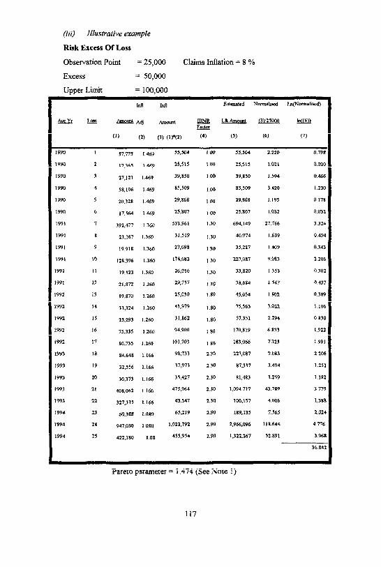
(iii) Illustrative example

Risk Excess Of Loss

Observation Point = 25,000 Claims Inflation = 8 %

Excess = 50,000

Upper Limit = 100,000

Infl Infl Estimated Nomalised Ln(NomaIised)

Acc Yr Loss Amount Adj Amount IBNR Ult Amount (3)/25000 In((6)) Factor

(1) (2) (4) (5) (6) (7)

1990 1 37,775 1 469 55,504 100 55,504 2.220 0.798

1990 2 17,365 1.469 25.515 1,00 25,515 1.021 0.010

1990 3 27,121 1.469 39,850 1.00 39,850 1.594 0.466

1990 4 58.196 1.469 85,509 1.00 85,509 3.420 1 .230

1990 5 20,328 1.469 29,868 100 29,868 1.195 0 178

1990 6 17.564 1 469 25,807 100 25.807 1.032 0.032

1991 7 392,477 1.360 533,961 1.30 694,149 21.766 3.324

1991 8 23.167 I.360 31,519 1 .30 40.974 1.639 0.494

1991 9 19,918 1.360 27,098 1.30 35,227 1.409 0.343

1991 IO 128.396 1.360 174,682 130 227,087 9.083 2.206

1991 II 19,123 I.360 26,016 1.30 33,820 I.353 0.302

1991 12 21,872 1360 29,757 1.30 38+684 1.547 0.437

1992 13 19,870 1.260 25,030 1.80 45.054 I.802 0.589

1992 14 33.324 1.260 41,919 1.80 75.563 3.022 1.106

1992 I5 25,293 1.260 31,862 I.80 57.351 2.294 0.830

1992 16 75,335 1.260 94,900 1.80 170,819 6.833 1922

1992 17 80,735 1.260 101,703 1.80 183,066 7 323 I.991

1993 18 84.648 1.166 98,733 2.30 227,087 9.083 2206

1993 19 32,556 I.166 37,973 2.30 117.337 3.494 1.251

I993 20 30,373 1.166 35,427 2.30 81,483 3.259 I.182

1993 21 4011,062 1 166 475,964 2.30 1,094,.717 43.789 3 778

1991 22 327,335 1166 43.547 1.30 loo.157 4.006 1.388

1994 23 60,388 1.080 65,219 2.90 189,135 7.565 2.024

1994 24 947,030 1080 1.022.792 2.90 2,966,096 118.644 4.776

I334 25 422, I80 1.08 453.954 2.90 1,322,267 52.891 3.968

36.842

Pareto parameter = 1.474 (See Note 1)

117

(3)-(1)*(2)

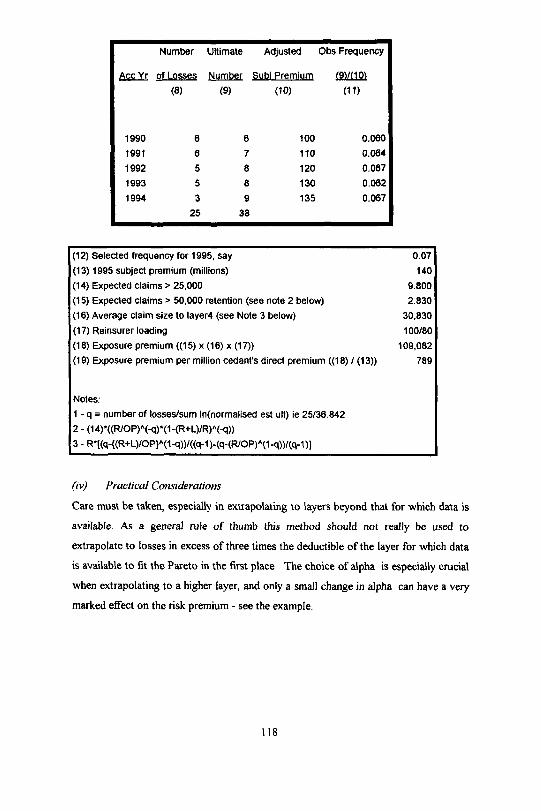
Number Ultimate Adjusted Obs Frequency

Acc Yr of Losses Number Subi Premium (9)/(10)

(8) (9) (10) (11)

1990 6 6 100 0.060

1991 6 7 110 0.064

1992 5 0 120 0.067

1993 5 8 130 0.062

1994 3 9 135 0.067

25 38

(12) Selected frequency for 1995, say

(I3) 1995 subject premium (millions)

(14) Expected claims > 25,000

(15) Expected claims > 50,000 retention (see note 2 below) (16) Average claim size to layer4 (see Note 3 below)

(17) Reinsurer loading (18) Exposure premium ((15) x (16) x (17))

(19) Exposure premium per million cedant’s direct premium ((18) / (13))

0.07

140

9.800 2.830

30.830

100/80

109,082

789

Notes:

1 - q = number of losses/sum In(normalised est ult) ie 25/36.842

(iv) Practical Considerations

Care must be taken, especially in extrapolating to layers beyond that for which data is

available. As a general rule of thumb this method should not really be used to

extrapolate to losses in excess of three times the deductible of the layer for which data

is available to fit the Pareto in the first place. The choice of alpha is especially crucial

when extrapolating to a higher layer, and only a small change in alpha can have a very

marked effect on the risk premium - see the example.

118

2 - (14)*((R/OP) (-q)*(1-(R+L)/R) (-q))

3 - R*[(q-{(R+L)/OP} (1-q))/((q-1)-(q-(R/OP) (1-q))/(q-1)]

Other curves may be appropriate to certain situations, and the lognormal might be used

if there are unlikely to be too many aggregations of losses, so that the tail of the

business is not too long.

The frequency at the observation point is used to infer the frequency at the retention,

and is often not the best guide to use. In practice, it can prove used to make

judgmental changes to the frequency at the observation point, effectively to treat the

Pareto as a two parameter distribution.

The Pareto has a fairly “thick” tail, and is usually censored. It does not fit well over

the full range of losses, and is only typically used for the upper tail of a given loss

distribution.

119

3.1.3 Exposure rating2

(i) Introductory remarks

Exposure rating is a technique for pricing X/L reinsurance which does not rely on the

availability of historical loss data. Instead the ceding company’s distribution of direct

premium by policy limit, (its “risk profile”) either current, or projected future, is used

together with, typically, increased limit factors (ILFs) for casualty business or Ludwig

tables for property or other published tables appropriate to a particular class and

territory, or a reinsurer’s own internal tables.

(ii) Basic recipe

For the class of business for which an X/L policy is to be priced, an estimate is needed

of the ceding company’s direct premium by policy limit over the period of cover. For a

Property cover, the first step would be to express the retention for the layer to be

priced as a percentage of each of the policy limits written by the cedant direct. The

retention plus the limit for the layer are then expressed as a percentage of each of the

direct limits in the same way. The former can be thought of as the proportion of each

policy limit being retained by the cedant, and the latter less the former as the

proportion of each policy limit which falls in the layer to be priced.

The next step is to choose appropriate values from Ludwig’s table of cumulative loss

amount distributions, depending on the class of business and type of coverage being

priced, for each of the percentages already calculated. For each direct policy limit, the

difference between the Ludwig values, multiplied by the direct premium for the limit

gives the expected value of the exposure premium for the limit falling into the layer

being priced.

For further details see “An Exposure Rating Approach to Pricing Property Excess of Loss Reinsurance”, Stephen J. Ludgwig, proceedings of the Casualty Actuarial Society, 1991.

120

2

This exposure premium must then be adjusted for

1. The portion of the direct premium in respect of losses,

2. The loss adjustment expenses to be allocated,

3. Any premium inadequacy,

4 Reinsurer’s expenses,

5. The absolute amount of direct premium projected to be written by the cedant

to get to a final exposure premium rate, per unit of direct premium written by

the cedant

For a casualty treaty, the method would be similar, but would use ILFs instead of

Ludwig values

(iii) Illustrative example

Example A

Property Exposure Rating Example,

Homeowner’s (Non-Catastrophe) Wind Losses: 150,000 xs 50,000

Allocated Loss Adjustment Expense Covered Pro-Rata to Loss

(1) (2) (3) (4) (5) (6) (7) (Retention 1 Value from Value from Exposure

Policy Subject Retention as Limit) (aS Ludwig Curve Ludwig Curve Premium

Limit Premium % of Pol Limit % of Pol Lim for (3) for (4) ((6+(5))‘(2))

100,000 4,000,000 50.00 % 200.00 % 0.980 1.000 80,000

300,000 3,000,000 16.67% 66.67% 0.951 0.986 160,000

500,000 2,000,000 10.00 % 40.00 % 0.934 0.976 84,000

750,000 1,500,000 6.67 % 26.67 % 0.892 0.966 110,500

1 ,000,000 2,000,000 5.00 % 20.00 % 0.871 0.959 176,500

2,000,000 750,000 2.50 % 10.00 % 0.860 0.934 55,000

13.250.000

121

612.000

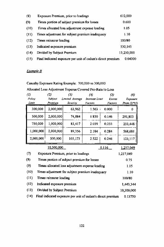
(8) Exposure Premium, prior to loadings 612,000

(9) Times portion of subject premium for losses 0.600

(10) Times allocated loss adjustment expense loading 1.05

(11) Ties adjustment for subject premium inadequacy 1.10

(12) Times reinsurer loading 100/80

(13) Indicated exposure premium 530,145

(14) Divided by Subject Premium 13,250,000

(15) Final indicated exposure per unit of cedant’s direct premium 0.04000

Example B

Casualty Exposure Rating Example: 700,000 xs 300,000

Allocated Loss Adjustment Expense Covered Pro-Rata to Loss

(1) (2) (3) (4) (5) Policy Subject Limited Average Increase Limit Excess

Text

Exposure Limit Premium Severity Factor Factor Prem (2)*(5)

300,000 2,000,000 63,962 1.563 0.000 0

500,000 2,000,000 74,884 1.830 0.146 291,803

750,000 1,000,000 83,417 2.039 0.233 233,448

1,000,000 2,000,000 89,356 2.184 0.284 568,681

2,000,000 500,000 103,173 2.522 0.246 Text

(7)

(8)

(9)

(10)

(11)

(12)

(13)

(14)

10.500.000 0.116 1.217.049

Exposure Premium, prior to loadings

Times portion of subject premium for losses

Times allocated loss adjustment expense loading 1.15

Times adjustment for subject premium inadequacy 1.10

Times reinsurer loading 100/80

Indicated exposure premium 1,443,344

Divided by Subject Premium 10,500,000

Final indicated exposure per unit of cedant’s direct premium 0.13750

122

1,217,049

0.75

(iv) Practical considerations

Exposure rating can be a usefultool, in particular in circumstances where little or no

historical loss information is available, so an experience rating approach cannot be

used. It can also be combined with experience rating into a credibility type approach

to pricing a layer of X/L.

Clearly care is needed in the use of, for example, the Ludwig tables, or the derivation

of ILFs to make sure they are appropriate to the coverage being priced.

In an ideal world excess of loss reinsurance rating should be a combination of both

experience rating and exposure rating. The rates under the different approaches are

unlikely to be the same, and the question of what weights are to attach to what

methods. This issue is addressed in “Credibility for Treaty Reinsurance Excess Pricing”

by Gary Patrick and Isaac Mashitz in CAS 1990 Discussion Papers on Pricing.

If both exposure and experience rates have been successfully estimated and they differ,

then there is a clear question of which to use. If the book has changed dramatically

over a period of time, then experience rating will be meaningless. If the future

exposure is likely to have changed, then the exposure rate is in doubt. In practice the

rate lies between the two.

123

3.2. Catastrophe excess of loss treaties

Introductory remarks

The available methods depend crucially on the information available, which varies

widely from territory to territory.

Good information is available in Australia where following the Darwin loss, the ICA

(Insurance Council of Australia) set up a detailed exposure tracking system.

Reasonable quality information is available from Cresta for earthquake zones for many

territories.

The data available for European Windstorm is generally moderate to poor, with

inconsistent monitoring of aggregates.

The UK flood is an example where historically information has not been available. This

may change with the publication of the Halcrow Report commissioned by the ABI and

other alternative studies being undertaken.

Information from United States is detailed.

It is of interest that the so-called developed territories are often worse at providing

aggregates information on a regular basis than those territories which are less well

developed.

Some markets have a Tariff rate for primary cover which may be used. The question

as to its adequacy may arise. For example, the rates for earthquake cover in Turkey

were set by the Government on the advice of a leading reinsurer so may be felt to be

reliable.

Information can be obtained from R&D departments of consultancies on damagability

and return periods of events.

124

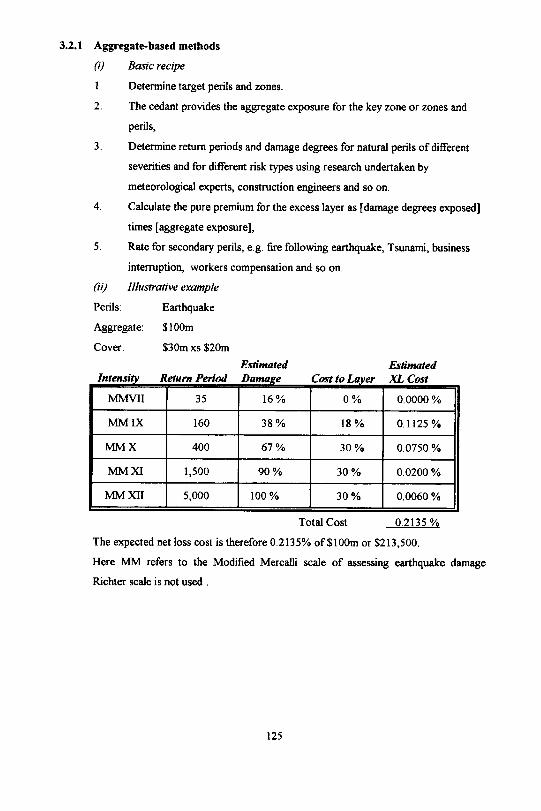
3.2.1 Aggregate-based methods(i) Basic recipe1. Determine target perils and zones.2. The cedant provides the aggregate exposure for the key zone or zones and

perils,3. Determine return periods and damage degrees for natural perils of different

severities and for different risk types using research undertaken bymeteorological experts, construction engineers and so on.

4. Calculate the pure premium for the excess layer as [damage degrees exposed]times [aggregate exposure],

5. Rate for secondary perils, e.g. fire following earthquake, Tsunami, businessinterruption, workers compensation and so on

(ii) Illustrative examplePerils: EarthquakeAggregate: $l00mCover: $30m xs $20m

Estimated Estimated

MMIX 160 38% 18% 0.1125 %

MMX 400 67% 30 % 0.0750 % I

MMXl 1,500 90 % 30% 0.0200 %

MMXII 5,000 100% 30 % 0.0060 %

Total Cost 0.2135 %The expected net loss cost is therefore 0.2135% of %l00m or $213,500.Here MM refers to the Modified Mercalli scale of assessing earthquake damage.Richter scale is not used

125

Intensity Return Period

Estimated

Damage Cost to Layer XL Cost

M M V I I 35 1 6 % 0 % 0.0000%

(iii) Additional examplesAn alternative method can be used for Australia where original gross premium is splitby zone, peril and coverage, Thus, the percentage relating to catastrophe ground upcan be determined and spread using a Pareto-type loss curve.Various studies for Caribbean windstorm have been undertaken to determinedamagability and return periods,(iv) Points in practiceCare must be exercised over the reliability of, and sensitivity to, the underlying returnperiod and damage assumptions. The choice of key zone is also problematic, especiallyfor windstorm exposures but also for earthquake. For instance, the impact ofearthquake in Mexico is very difficult to model. This is because Mexico City is builton landfill, surrounded by mountains which amplifies the earth’s movements; a quakefalling in this mountainous area will therefore cause a higher degree of damage to thecity than at its epicentre. The 1985 Earthquake had its epicentre in the PacificPremium is independent of market and cedant rates.The need to understand original coverage, coinsurance and deductibles make thepractical application very difficult.

3.2.2 Loss based methods(i) Basic recipeObtain the historic loss amount from specified events,Revalue for inflation,“As if’ for changes in the portfolio//exposure,Assign return periods to the catastrophic events,Add “ghost” events and return periods outside historical experience.(ii) Illustrative examples“90A” for UK wind,Typhoon 19 Mireille for Japanese wind.(iii) Points in practiceA common problem can be rating for one event only. There is the need to recognisethat two or more events are possible. Some lower layer catastrophes are effectivelysecond loss policies.

126

32.3 Simulation/modelling methods(i) Basic recipeObtain the cedant exposure split by postcode, prefecture, etc.,Determine a distribution of events with data either from external consultancies or aninternal R&D department. This will need frequency and severity components, togetherwith an implied damage ratio for each severity.,Run a 1,000 year simulation, say. It is better to use stratified than random sampling tocope with the rare events. A good example is the Latin Hypercube sampling used by“Crystal Ball”. Monte Carlo simulation does not have this feature, and could lead tounderpricing.Determine the average and standard deviation ( and possibly higher moments) oflosses to the layer concerned.(ii) Illustrative exampleThe output of a simulation on a UK property account is part of Appendix 2 to thispaper. This has been achieved by using a commercially available package. As analternative see “Storm Rating in the Nineties” [21].(iii) Points in practiceVery complex and subjective modelling is necessary,Packages can be bought in the marketplace.(iv) ExampleHistorically in the US the following procedure was used:Establish the total wind exposed premium. This was a percentage of total premiumvarying by line, e.g. 25 to 30% for homeowners or 7½ to 10% for auto propertydamage.Apply a 20% PML. This gave the attachment point for a reasonable catastropheprogramme for which a rate on line of 20 to 25% would be charged. Higher layerswere then priced at around two-third of the previous layer and experience adjustmentswere made.However, following the 1989 Hurricane Hugo loss rates increased dramatically. Thisled to pressure from carriers who were less exposed to refined pricing methods,

127

The simulation programme CATMAP is now widely used. This at a standard levelruns off the income split by State, but enhanced versions use a county or even zip codebreakdown. The results cover wind and earthquake exposure, but an additional loadneeds to be made for other perils such as riot, flood and terrorism, or additionalcoverages such as California workers’ compensation or business interruption.Other packages are available for UK and other territories.

3.2.4 Burning Cost Rating

Under Burning Cost Rating actual losses incurred are used to determine the cost. Thekeys to assessing these rates are:-(a)

(b)

(c)(d)

Loss FrequencyA burning cost method is only suitable if there are a sufficient number of lossesto obtain a suitable loss frequency.lndexationLosses should be revalued into current terms. This involves both inflation andthe increase in number of policies. A suitable index could be premium incomeadjusted for any rate changes.Changes in Policy ConditionsChanges in Retention

3.2.5 Exposure RatingExposure rating is used to rate areas and covers with little or no loss experience. Thereare three stages:-(1) Establish a Catastrophe Estimated Maximum Loss (E.M.L.).(2) Establish a Catastrophe Premium - this is normally From The Ground Up -

(F.G.U.).(3) Establish a suitable Loss Distribution Curve. A Pareto type distribution is the

norm, although this is derived frorm “feel” rather than parameters, due to thelack of data..

128

Set out below is an example of a calculation for a UK direct writer requiring a quote of£25 million excess of £50 million. Reinstatements and brokerage are ignored. This isbased on a 1992 quotation.The estimated Gross Premium income for 1992 is £230 million and the loss data is asfollows:

1984 145,000,000 6,500,000 10,310,344

Premium F.G.U.Losses Indexed

1991 220,000,000 Nil Nil1990 200,000,000 95,000,000 109,250,000 (90A)

22,000,000 25,300,000 (90D)1989 180,000,000 Nil Nil1988 170,000,000 Nil Nil1987 160,000,000 65,000,000 96,451,612 (875)1986 155,000,000 Nil Nil1985 150,000,000 Nil Nil

1983 120,000,000 NilNil1982 1,00,000,000` Nil Nil

First calculate the Maximum Possible loss. This is assumed to be twice the 90A LossIndexed i.e. £220 million (2 x 109.250). This is based on “current market practice.”Flood damage is not considered, but could give rise to a substantially higher PML.Next, we calculate a loss for a specific layer. The practice is to use 90% xs of 10% ofthe largest loss (109,250,000) say £90 million xs £10 million.The losses to this treaty at the current index would be £90 million + El 5. 3 million +£86,`451 million + SO.310 million = £192.151 million (This is similar to the burningcost). The average cost is £19.215 million per annum.This cost, from the Pareto curve, represents about 50% of the total cost. This is takenfrom the size of loss curve below looking at the size of loss of 10 (giving 20%) and 50(giving 70%). Therefore, the total catastrophe programme should cost £38.42 million.

129

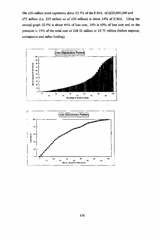
The £50 million point represents about 22.5% of the E.M.L. of £220,000,000 and£75 million (i.e. £25 million xs of £50 million) is about 34% of E.M.L. Using thesecond graph 22.5% is about 45% of loss cost, 34% is 60% of loss cost and so thepremium is 15% of the total cost of £38.42 million or £5.73 million (before expense,

commission and safety loading).

130

3.3 Proportional treaties(i) Introduictory remarksTraditionally, the attitude of “follow the fortunes” meant that the only pricing decisionwas how much over-rider commission to add to the cedant’s original commission. Inrecent years, poor underlying performance, and growing recognition of the unlimitednature of the cover and the extent of natural perils exposures, have led reinsurers tomake their own assessment of the total reinsurance commission affordable,independent of the original commission This section will use a property proportionalexample to illustrate the ideas, then discuss application to other lines of business.(ii) Basic recipe1. Split the exposure into three separate components:

Basic loss cost (ordinary losses)

2.

Large individual fire losses (peak losses)Catastrophe/event losses (natural perils losses),

The basic loss cost may be priced using normal burning cost/experience ratingmethods as follows:a) Take the 100% cost of claims to the treaty for the last 5 or 10 years,

and subtract peak and natural perils losses above a certain level, toobtain the experience of ordinary losses

b) Put the historic experience onto an “as it" basis of the currentexposures, e.g. adjusting for changes in primary underwriting terms andconditions, changes in portfolio mix and any other appropriate factor,

c) Revalue the experience to reflect claims inflation and changes inprimary rates.

d) Take a suitable average or trend of historic experience, to arrive at anexpected basic loss cost for the forthcoming treaty year.

131

3. For peak losses, a suitable deductible is chosen The cost of claims below thislevel falls into the basic loss cost. The cost of exposure to claims above thislevel should be priced using normal risk X/L methods, e.g.:

a) Obtain a risk profileb) Use a loss curve to apportion the original premium to exposures above

and below the deductible.c) If a risk profile is not available, you may be able to use a Pareto curve

extrapolation of the recent large loss history, but this is less satisfactoryd) upper limit equals treaty maximum sum insured.

4. Catastrophe losses should be priced using a normal X/L method of ratingsuitable to the risk and territory concerned:a) The choice of deductible will depend on the territory and perilSometimes the cedant will only report natural perils losses above a certainamount, e.g. minor snow/freeze losses in the UK, e.g. minor typhoons inSE Asia. Sometimes the cedant will report all losses, and the peril should berated from the ground upb) The upper limit can be chosen as the event limit if the treaty is capped,

otherwise treat as an unlimited treaty.c) If the cedant is using cession limits, the reinsurer needs to be very

confident of the basis before using this as a pricing cap.d) Then use normal aggregate or loss based methods, consistent with

rating X/L exposure in the same territory.

e) Often there will be a tariff in the territory for the natural perilconcerned, e.g. earthquake in Turkey, and the primary premium will besplit between natural peril and fire premium, with different commissionscales. The reinsurer should obviously make himself aware of thesource of the tariff, and in the spirit of proper pricing be prepared totake a different view.

(iii) IIIustrative exampleThe separate components of basic loss cost, peak loss cost and natural perils cost areall calculated using similar techniques to those shown in the X/L sections,

132

(IV) References for further reading“The Rating of Pro-Rata Treaties”, LIRMA 1994, gives a clear exposition of theprinciples, and a long worked example,“Property Insurance: Data Requirements for Calculating Correct Premiums inInsurance and Reinsurance”, Munich Re 1990, covers other topics as well, but showsin great detail the degree of information reinsurers should ideally require from cedants.

v) Points in practiceUnderwriters now find that, given the information requirements and the variety oftechniques involved, pricing a proportional treaty is often harder than pricing an X/Ltreaty. Given the relative premium volumes, and the greater uncertainty on exposures,they should not be surprised!Other issues include variable commission scales, Loss participation clauses (LPC) andloss corridors, event limits (cf. cession limits), and the cashflo wmechanics of differenttypes of commission scale

133

3.4. Use of simulation methodsi) Introductory remarksUsed for calculations in the following circumstances:Special treaty conditions depending on the aggregate amount of losses:

Aggregate deductiblesReinstatement premiumsSliding scale commissions on pro-rata treatiesSliding scale premiums on risk X/L treaties (“swing rates”)Profit commission,

Treaties with special coverages depending on the aggregate amount of losses:Loss corridorsLoss participation clausesCovers with aggregate annual limitsTotal loss only covers.

(ii) Basic recipeAssess the loss cost for the ordinary cover without the special conditions, using thenormal techniques,Analyse the ordinary loss cost into separate components of frequency and severity,Assume a suitable distribution for each of these components, e.g. Poisson forfrequency and Pareto or lognormal for severity,Using this model of the loss cost, simulate the result of, say, 1,000 years of experienceof the coverage with the special conditions included using, say, the @RISK add-onpackage,Care should be taken over the treatment of expense and profit loadings:Calculate amount of loading on the original premium. This should be a cash amountaddition to special premium, not a percentage loading.(iii) Illustrative exampleSuppose you have a cover £0.5 xs £0.5, where the ordinary loss cost (beforeloadings) is 1 15% of GNPI of £1000, i.e. you expect about 4 to 5 losses to hit thelayer, and the cedant asks you to quote for the cover with an annual aggregatedeductible of £1m,

134

Assuming the exposure is per risk only with no event exposure, then re-express thepremium basis as:a.) expected frequency of 5.0 losses p.a. to the layer, modelled as having a Poissondistributionb) severity is Pareto with alpha of 2.3These parameters might come directly from the original rating calculation. If they arenot available, for example, because an experience method was used, it is probablyinstructive to estimate them from the data as a first check of the result.Then it is very simple to model the cover with the deductible in @RISK, which showsthe new loss cost is £0.34m, i.e. the credit for the deductible is £0.81m, i.e. 81%.If the original loadings for expenses and profit had been (100/75), i.e 33%, the newpremium should be loaded with £0.38m (33% of El .15m), not £011.m (33% of£0.34m).Further examples are given in section 4.3 on stochastic profit testingFor simulating catastrophic events alpha stable distributions are being considered SeeAppendix 1.2

135

3.5. Stop-loss treaties

(i) Introduction

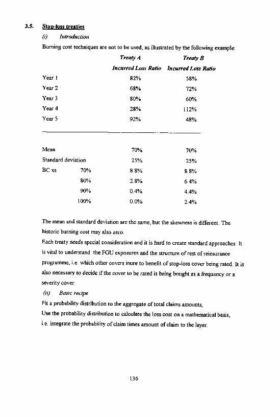
Burning cost techniques are not to be used, as illustrated by the following example:

Treaty A Treaty B

Incurred Loss Ratio Incurred Loss Ratio

Year 1 82% 58%

Year 2 68% 72%

Year 3 80% 60%

Year 4 28% 112%

Year 5 92% 48%

Mean 70% 70%

Standard deviation 25% 25%

BC xs 70% 8.8% 8.8%

80% 2.8% 64%

90% 0.4% 4.4%

100% 0.0% 2.4%

The mean and standard deviation are the same, but the skewness is different. The

historic burning cost may also zero.

Each treaty needs special consideration and it is hard to create standard approaches. It

is vital to understand the FGU exposures and the structure of rest of reinsurance

programme, i.e which other covers inure to benefit of stop-loss cover being rated It is

also necessary to decide if the cover to be rated is being bought as a frequency or a

severity cover.

(ii) Basic recipe

Fit a probability distribution to the aggregate of total claims amounts,

Use the probability distribution to calculate the loss cost on a mathematical basis,

i.e. integrate the probability of claim times amount of claim to the layer.

136

Ideally, you would like to create separately distributions for both frequency andseverity of the underlying primary experience, but you may have to fit it against as-ifhistorical loss-ratio experience.

(iii) Illustrative exampleConsider a medium size specialist UK insurer seeking a stop-loss on its household andsmall business property account. The natural perils losses were subtracted from theexperience of the last 20 years. Once the residual experience was revalued, it wasquite clear that there was an underlying cycle. Instead of taking the plain arithmeticalstandard deviation, the variability about a suitably modelled trend was assessed. Thiswas used to model an expected trend loss ratio for underlying claims, and variabilityaround the trend.The catastrophe exposure was modelled separately, using a loss-based method giving adistribution of return periods for events of different sizes,The two separate distributions were combined using @RISK, which allowed thepricing any desired stop-loss cover.(iv) References for furher reading“On the Rating of a Special Stop Loss Cover”, G. Benktander, ASTIN 1974.(v) Points in practiceCare over treatment of expense and profit loadings.In excess of loss reinsurance rating, only 5 years of statistical information is normallyused. In stop loss, you need a much longer period, desirably 20 to 25 years. It ispreferable to have covers where the fluctuation comes from the claims side and not thepremium side, e.g. hail or windstorm.

137

3.6. Credibilitv Theory

3.6.1 Much has been written about Credibility Theory in Actuarial and Risk TheoryLiterature. Interested readers can refer to [IS] and [ 16] for further and more detailedinformation. This section highlights aspects of Credibility Theory that are sometimesused in the London Market albeit often without the knowledge of the user.

3.6.2. Consider the following scenario, You need to charge a premium for a risk where youeither have :-1. No loss data for the risk (e.g. a new building); or2. Some loss data relating to the actual risk.In the first case you may end up charging what is perceived to be the “Market Rate”for the exposure unit appropriate for the class with perhaps some subjective allowancefor the feel of the risk; for example the quality of the risk management, the quality ofthe business the broker usually shows you, the current market cycle, and so on. In thesecond more common scenario we are faced with some further additional questions:-1. What use are we to make of the loss history presented to us ?2. Is the data relevant to the loss experience going forward ?3. Is other collateral data relevant to the risk, and if so, what use can we make of

it ?

3.6.3 In essence, we want to incorporate an allowance for both the collateral data relating toother similar risks and to the individual assureds loss experience. Ignoring expenses,commission, profit and other loadings we wish to arrive at a premium based on

P = z* + (1-z)*µ (1)P = premium = price based on loss experience onlyZ = Credibility weightµ = price based on collateral data only

3.6.4 Applying equation (1) to the above two examples, Z takes the value 0 in the first caseas no weight is given to the individual assureds historic loss experience. Moreover, theabsence of any historical loss experience may lead to an extra element of doubt in theunderwriters mind and would thus lead to an extra risk loading on the overall premium.

138

Case 2 requires a lot more effort in arriving at an appropriate credibility factor Z forthe risk in question. There are some natural constraints on the value.1. Z can only take values between 0 and 1.2. The more data we have for the risk, the more weight we should attach to the

insured’s historic loss experience, i.e. the larger Z.3. The less relevant the collateral data, the less weight we should attach to it, i.e.

the larger Z.4. The more the underwriter feels the claims process going forward is likely to be

similar to the past, the larger the value of Z.This naturally leads to the question of how much data is needed before full credibility isascribed, i.e. Z equals 1.

3 6.5 The criterion used by some North American actuaries to determine the amount of dataavailable from the risk under consideration was sufficiently large for Z to be taken asunity was that the relative error between the true pure premium and that estimatedbased on historical data alone should be less than some given amount with some givenprobability. The terminology used is that the data set is Fully Credible (k,p) if the datasize is such that the probability of the pure premium estimate is p percent certain ofbeing within k per cent of its “required” value. Numerical examples are given in [ 16].When full credibility is not available, partial credibility results in Z being less thanunity. There are a few ad-hoc methods employed to assign a value to Z, for example

n = number of claims in loss historym0 = number of claims required for full credibility

This formula has the advantage that it is easy to understand and has some statisticaljustification if we are looking at a risk whose aggregate loss distribution is compoundPoisson.

3.6.6 Empirical Bayes Credibility TheoryThis is a useful branch of credibility theory which has practical uses in premium ratingwhere you have loss and exposure data for similar risks. Consider the data in theexample which relates to the number of losses for various hospital trusts in a particular

139

American State, We wish to estimate the expected loss frequency for the forthcomingpolicy year.Y,, represents the number of losses experienced by hospital i in year jP, represents the exposure measure for hospital i in year jx‚‚ therefore represents the loss frequency per unit of exposure for hospital i in year j

and equals Y‚‚IP‚‚We wish to estimate the loss frequency for one or more hospitals in the state for theforthcoming year The process used will allow us to use the collateral data availablefrom other hospitals which can be expected to exhibit similar but probably not identicalloss frequencies.

3.6.7 The assumptions underlying the Empirical Bayes Credibility Theory Model are1. xij are independent for j = 1,...,n

The distribution of Xij depends on the value of whose value is fixed butunknown Xi,!01, Xi2 01 are independent but not necessarily identicallydistributed,

2. 3. are independent and identically distributed.

If we assume that there are functions m( ) and s( ) such that(2)(3)

Rewriting equation (1), our estimate of loss Frequency will be in the form :-Loss frequency = z1 × x1 + (1-Z1) × E[m( )] (4)

IF we further define

It can be shown that the estimates for the credibility frequency are

140

The Paris and are independent for i#k

where

3.

3.6.8 Example

Hospital Yij

1234567

pij j Total Exposures (OBU)

Total

Yij/Pij

2

YearTotal Number of Claims1 2 3 4

520 464 400 380178 188 150 145100 88 89 110200 189 212 230300 250 340 19950 80 100 8940 60 61 59

18000350013223750645440001215

28241

2 3 4 57500 7454 8125 85654512 4156 4878 42101566 1787 1714 15003600 3500 3700 37826544 4959 5252 57454152 4565 4755 65001515 2000 1858 1959

29389 28421 30282 32261

542520012522528811062

1 2 3 4 50.065 0.062 0.054 0.047 0.0500.051 0.042 0.036 0.030 0.0480.076 0.056 0.050 0.064 0.0830.053 0.053 0.061 0.062 0.0590.046 0.038 0.069 0.038 0.0500.013 0.019 0.022 0.019 0.0170.033 0.040 0.031 0.032 0.032

It follows from the above equations that = 148594P* = 3596,93 = 0.0451

Whence

141

j

1234567

1234567

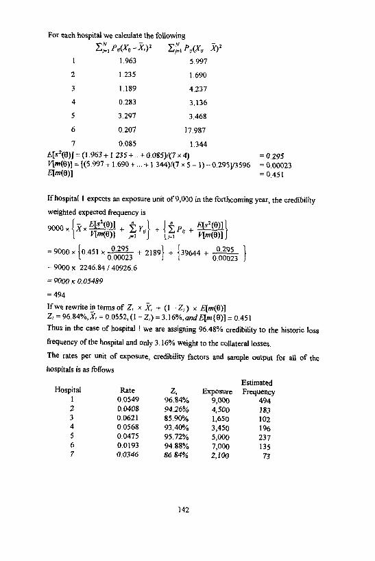
For each hospital we calculate the following

1 1.963 5.9972 1.235 1.6903 1.189 4.2374 0.283 3.1365 3.297 3.4686 0.207 17.9877 0.085 1.344=(1.963+1.235+..+0.085)/(7×4) = 0.295=[(5.997+...+1.344)/(7×5-1)-0.295]/3596 = 0.00023

= 0.451

If hospital I expects an exposure unit of 9,000 in the forthcoming year, the credibilityweighted expected frequency is

= 9000 x 2246.84 /140926.6= 9000 x 0.05489= 494If we rewrite in terms of z1× X1 + (1 -Z,) x E[m( )]Zi =96.84%,Xi = 0.0552,(1-Zi)=3.16%,andE[m{ )]=0.451Thus in the case of hospital ! we are assigning 96.48% credibility to the historic lossfrequency of the hospital and only 3.16% weight to the collateral lossesThe rates per unit of exposure, credibility factors and sample output for all of thehospitals is as follows

Hospital Rate Zi Exposure1 0.0549 96.84% 9,0002 0.0408 94.26% 4,5003 0.0621 85.90% 1,6504 0.0568 93.40% 3,4505 0.0475 95.72% 5,0006 0.0193 94.88% 7,0007 0.0346 86.8% 2,100

EstimatedFrequency

49418310219623713573

142

3.6.9 Robust CredibilityAnother problem in assessing credibility is the existence of outliers, i.e. extreme eventswhich, although appearing in the data, should be initially ignored for the purpose ofrating. A paper by Gisler & Reinhard in Bulletin of ASTIN gives a solution to part ofthe problem. In this paper they deal with loss ratios, Previous methods of treatingextreme loss ratios is to apply trimming at some percentage point, and to “distribute”the excess losses over the whole portfolio by an appropriate loading. The questionarises as to the level of such trimming.

3.6.10 The real aim is to limit the influence of large claims on the data, and this is the directaim of Robust Statistics Theory. The combination of Robust Statistics and CredibilityTheory gives us Robust CredibilityIn their paper Gisler & Rheinhart apply the mathematics of Robust Credibility to claimswhich act in accordance with the general Buhlmann Straub model ( which is similar tothe Bayesian technique given above.

Let Xij be the anticipated loss ratio for policy i in year j.

Let Ti be the credible loss ratio for the upper trimming of data(Note that the paper does not consider trimming low loss ratios )

The calculations give a loss ratio as follows

3.6.11 Alternatively, the estimate for the rate is calculated by trimming the loss ratio at twicethe expected value. Ti is solved by iteration.The paper does not deal with the use of low cut off points (i.e. where loss ratios in oneyear are exceptionally low) and as far as we are aware there is no solution to theproblem. It has been suggested that the truncations form a pair (Tb , Tb ) where Tbrepresents the lower bound and Tb the upper bound. (0, 2Ti ) is just one suchpairing.This sort of approach may be considered against (say) the background of swing rated(or experience rated ) business where upper and lower limits are placed on the baserate to accommodate variation in the loss ratios.

143

3.7 Distribution Calculus methods

Distribution calculus is an important method in assessing rates for risk excess

reinsurance The basis is to start with a number of individual (or grouped) claims over

either one or more years. Technical details such as indexation, and how to deal with

incomplete sets of data need to be addressed (truncated or censored data).

From this data set an empirical loss distribution is devised. Then, using maximum

likelihood methods or similar statistical approach, a Fitted Distribution is calculated

which may extend the empirical distribution to allow for the possibility of claims in

excess of those recorded. The distribution selected may be more prudent than the

empirical data.

The next stage is to calculate the aggregate loss distribution for the layer. This is

achieved by recursive algorithms which are documented in many papers, and in

particular [6]. The method is as follows

1. Determine the distribution of claim size.

2. Determine the lower limit (truncation point) and upper limit (censor

point).

3. Use an appropriate claims distribution, often determined by the first three

moments (mean, variance and skewness).

4. The distribution is calculated, and in particular the expected value and

variance, and these are then input into the appropriate rating formula to

calculate the rate.

The algorithms are readily available in computer programmes, and are relatively easy

to apply

144

3.8 Generalised Linear Interactive Models (GLIM)

3.8.1 Generalised Linear Interactive Models are used in those cases where there is a

substantial volume of individual data and well defined rating factors. As such their use

in pricing London market business is very limited. The use of the GLIM algorithm is

well documented in recent actuarial papers and in text books. Examples of London

market business where it is of use include Motor Classes, Marine Hull, Marine Cargo

and P&I Clubs.

3.8.2 GLIM models are normally applied to large data sets that can easily be classified into

constituent rating groups. The algorithm then seeks to apportion the extent that the

expected loss cost was related to the individual rating factors. Individual rating factors

could be eliminated from the pricing process if their contribution to the expected loss

cost was not significant. i.e. they do not significantly improve the fit of the model. The

“best” model would then be the one which produced the nearest approximation to the

data based on the least number of rating factors.

3.8.3 As an example , for Marine Hull business, losses could be categorised by Age,

Tonnage, Type of Vessel, Location of Loss and so on. A Linear Model is then fitted to

this, and careful consideration must be paid to any interactions that may exist, for

example between Tonnage and Age, and also the uneven distributions in the database.

Oil Tankers below 40,000 tonnes are rare, as are Tugs over 15,000 tonnes.

145

4. STRATEGIC PRICING

4.1 Introduction

This section of the paper describes the various components of an approach to pricing

under the heading of “Strategic Pricing”. It is considered that the pricing/underwriting

objectives must fall within the company’s overall objectives. These are usually

formalised when a corporate plan is prepared setting out the direction of the company

over the planning horizon, The plan may consider the type of business the company

wishes to write and the capital required to support that business. Certain underwriting

results after expenses would be required from the business written which together with

any investment income should be sufficient to provide the required return on the

capital and to generate sufficient surplus to meet any growth targets included in the

plan.

The methodology described in this section may be used in many different ways, for

example to :

a) Provide input on price determination of large risks

b) To set portfolio pricing objectives

c) Input into strategic planning

d) As part of the control cycle

The above uses of pricing are each considered through the application of profit test

methodology allowing for the time value of money, risk/reward and other assumptions

to determine the true profitability of a particular tranche of business.

There are two main approaches when considering pricing

Approach 1 - Empirical Pricing by Individual Risk

Take an estimated loss ratio derived using more traditional techniques and then apply

profit test logic to determine the true profitability of the business, probably using a

Return on Capital (ROC) type measure. Revise underwriting approach if the result id

not what is required. This approach is useful when trying to price a particular risk,

where allowances for individual risk characteristics may be made, for example

premium receipt patterns, level of excess,

146

Approach 2 - Portfolio Pricing Targets

Make assumptions about the required return, investment return and so on to determine

the required ‘target’ loss ratio which is needed to satisfy shareholders’ objectives. This

approach is useful when considering a collection of risks together at various levels.

Section 4.2 describes the links between underwriting targets, pricing and reserving.

The processes involved in determining the underwriting targets and pricing and

accepting new business are outlined. The underwriting performance measurement in

the form of reserving and monitoring plan variances are then described. This is

followed by description of early warning systems and feedback loops whereby the

latest available information is made use of in the planning and pricing decisions for the

subsequent periods.

Section 4.3 describes the processes involved in segmenting the business, measuring

risk variability of different classes of business and in determining the capital required to

support a given level of business. The processes involved in determining risk weighted

return on capital are then described. The determination of capital requirement to

support business written is related to the concept of risk based capital which looks at

the company from the solvency perspective.

Section 4.4 describes the concept of profit testing. The concept is described in outline

including the various assumptions, cash flow projections and scenario testing. The

section also illustrates the concept for a simplified class of business.

Section 4.5 covers the topic of underwriting management. This includes problems

encountered in managing the underwriting cycle and detailed consideration of factors

influencing underwriting targets, balancing the portfolio and risk selection.

147

4.2 UDERWRWRITING TARGETS & CONTROL CYCLE

4.2.1 Introduction

This part of the paper describes the links between underwriting targets, pricing and

reserving. The processes involved include reserving, tracking the business written and

establishing feedback loops whereby the latest available information is made use of in

the planning and pricing decisions in the subsequent periods. The process may be

schematically described by the following diagram:

4.2.2 Planning over a time horizon

A reinsurance company may prepare a business plan over one year, three year, or

possibly even longer time scales. A one year plan considers the underwriting targets for

the forthcoming year and has an immediate impact, whereas a three year plan allows

longer term strategy and direction to be considered. A five year or longer term plan

may be less common in the London Market, but could be beneficial if it was possible to

forecast the underwriting cycles, which have historically tended to repeat over five-six

year time periods.

The business plan makes best assumptions about the levels of business expected to be

written. These may be based on capital allocations and required return on capital,

allowing for market conditions and expected developments over the plan period.

The assumed losses may be based on weighted loss ratios for the significant business

within each portfolio allowing for any market trends. The loss ratios may be those

given by the pricing models, either conventional or profit testing models described

later. It is possible that such loss ratios may be inconsistent with those required to

148

achieve the return on capital, in which case such inconsistency may have been accepted

in view of longer term strategy considerations or it may be intended to achieve the

target loss ratios by actively managing the portfolio. These issues are considered in

detail later on in the paper.

The plan will make other assumptions such as expense levels and investment income.

The plan may also consider cash flow projections which involve assumptions about

premium and paid loss developments. Any such assumptions should be consistent with

those used in the profit testing and pricing models.

4.2.3 Pricing & accepting new business

The underwriter may carry out pricing calculations and accept/reject business using

either the conventional methods, profit testing models, application of judgement, or a

combination of methods.

He will have the underwriting premium targets in mind since his performance may be

measured against these targets. If the market conditions are less favourable than

anticipated in the plan then the underwriter will be faced with difficult decisions. It is

also possible that the plan assumptions may have been overtaken by subsequent events,

e.g. a large catastrophe in the interim significantly affecting the market conditions.

There may also be new opportunities not envisaged in the plan.

The underwriter may be constrained by guidelines on limits by contracts, programs

( groups of contracts within a class of business), reinsureds, class of business and

countries. The underwriter will also have limits by individual events or perils and

aggregate exposure to such losses by individual territories. Such limitations may be

determined by the existence of outwards reinsurance program and the nature and terms

of such program.

The underwriter will went to make effective use of the capacity available and will want

to ensure that he leverages the capacity for catastrophe business to get better deals

with individual reinsureds on other classes of business

Some of these issues are considered in more detail later in the section 4.5 of this

paper on “Underwriting Management”.

In any case at the time of underwriting a risk, there will be more up to date information

available relating to the market as a whole and the experience of the individual risks

149

being underwritten. There may also be more up to date information available in respect

of historic underwriting years relating to the class of business.

More and relevant the information available to the underwriters the better the

underwriting decisions that can be made. The quality and the timeliness of the

appropriate underwriting information can make the difference between profit and loss

when the market conditions are difficult and competitive.

4.2.4 Reserving

The reserving process may be considered as periodic evaluation of the underwriting

performance. The process makes use of the known information together with

assumptions about the unknown. The experience is then tracked and the assumptions

are modified in the light of the emerging experience.

When no historic credible data is available, the reserving process effectively starts with

the plan assumptions, The reserves are based on up to date premium estimates, the loss

ratios assumed for the plan and allow for the expected development patterns of

premiums, paid losses and incurred losses. The development patterns may be based on

the company’s own experience for previous underwriting years adjusted for any

available market statistics.

If the actual reported losses are adverse compared to the expected losses, the adverse

movement may be investigated in more detail to determine scope for further

deterioration and the plan reserves may be strengthened accordingly.

Thus in the reserving process, more up to date information becomes available at the

portfolio level. This information may shed light on deterioration in any risk factors

used in the pricing process, Information may become available on how the historic

years are materialising and if any marked changes have occurred in premium and loss

development patterns. In analysing adverse loss movements, further information may

become available on individual large losses, or losses by regions or for individual

reinsureds.

In some instances, such matters may be discussed extensively with the underwriters so

that they too are more aware of how the business written in more recant years is

performing.

150

4.2.5 Monitoring variances in Underwriting Targets

The actual experience will be monitored against the underwriting targets. The variance

will be analysed in detail and explained so that the information can be used in future

plans.

As more up to date information becomes available about the market conditions, terms

of trade and the business actually written, it may be possible to draw conclusions from

this information about how the current year is likely to materialise.

New information about losses from the current year and historic years will become

available from the reserving process described above. In addition, more up to date

information about outwards reinsurance costs and expenses will become available as

well as any changes in exchange rates and investment returns

Efficient collation and use of such information as it becomes available not only gives

advance indicators of the potential profitability of the year as a whole, but also gives

information as to validity or otherwise of the assumptions made in the planning and

pricing models. This enables any significant changes in the underlying assumptions to

be considered and immediately reflected in the subsequent pricing decisions.

Such information would also enable the company to take corrective measures relating

to types and levels of business to be written and to achieve more effective control and

use of resources.

4.2.6 Early warning systems

In the process of monitoring the variances in the underwriting targets, information will

come to light on various risk factors which are likely to have an impact on the business

development, Use of the information from the reserving process combined with

effective management information systems will give early advance indicators about

favourable or adverse developments. The use of this information would enable the

company to achieve the business development in a controlled environment.

Some of the risk factors which would be closely monitored are aggregate exposures,

rates of premium growth, trends in loss ratios and reasons for any adverse movements,

effectiveness of the reinsurance program, trends in expense ratios and acquisition

costs, and investment returns.

151

Effective management information systems would enable the above risk factors to be

analysed and tracked at a detailed constituent level so that the effect of the changes at

individual class/risk level can be assessed as well as the combined effect on the

business as a whole.

4.2.7 Feedback loops to Underwriters I Senior Managers

At a micro level, the actuary would talk to the underwriters/claims staff about

experience of a class at a portfolio level or of individual risks in order to understand

the business, so that the reserving process can be made more effective. When exploring

adverse movements, the actuary will gain an insight into the underlying risk factors

which can then be incorporated into any pricing models. The actuary can also give the

underwriters useful information at the portfolio level so that the underwriters can

better appreciate the effect of their underwriting decisions on the financial results.

Any sophisticated pricing models incorporating various risk factors and financial

considerations may assist the underwriters in identification of the obviously good and

bad risks so that they can focus on the more difficult and complicated risks. The

actuary can also assist the underwriters with the larger risks which have significant

financial impact and where a different perspective may he useful and justified.

The actuary will also be involved at the macro level in investigating the business

experience and presenting the actuarial report to the senior managers. At such

presentations the actuary may report on variances against plan, the reasons for the

variances and any corrective measures required. The senior management meeting may

also address longer term strategy issues on capital allocations, return on equity, levels

and classes of business to be pursued, effective resource management, investment and

taxation matters, cash flow management and dynamic solvency

The actuary is well positioned to participate in both micro and macro levels since he

has the relevant skills and knowledge to communicate effectively at both levels.

152

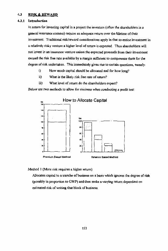
4.3 RISK & REWARD

4.3.1 Introduction

In return for investing capital in a project the investors (often the shareholders in a

general insurance context) require an adequate return over the lifetime of their

investment. Traditional risk/reward considerations apply in that to entice investment in

a relatively risky venture a higher level of return is expected. Thus shareholders will

not invest in an insurance venture unless the expected proceeds from their investment

exceed the risk free rate available by a margin sufficient to compensate them for the

degree of risk undertaken. This immediately gives rise to certain questions, namely:

i) How much capital should be allocated and for how long?

ii) What is the likely risk free rate of return?

iii) What level of return do the shareholders expect?

Below are two methods to allow for riskiness when conducting a profit test:

to Allocate Capital

Allocates capital to a tranche of business on a basis which ignores the degree of risk

(possibly in proportion to GWP) and then seeks a varying return dependent on

estimated risk of writing that block of b u s i n e s s ,

153

Method 1 (More risk requires a higher return)

isk

Method 2 (More risk requires more capital backing)

Allocate variable amounts of capital dependent on the estimated level of downside risk

associated with writing a particular tranche of business but seek the same return to

shareholders for all capital invested regardless of where.

Empirically Method 1 would appear to be sensible, however under this method it is

less clear what the maximum amount of business is which could be supported by a

given amount of financing Furthermore the relationship between risk and return for

various tranches of business needs to be determined in the form of percentages.

Like Method 1, Method 2 also needs to determine the relationship between risk and

return but this seems more straightforward in that the impact on capital of certain

downside risks is easier to contemplate (e.g. the impact on capital of a major

catastrophe say once in 10 years). As in practice most insurance concerns will know

reasonably accurately what their current available capital is, it is straightforward to

determine the implications on maximum premium volume of a given capital allocation.

Ideally the absolute level of risk needs to be determined for each class being modelled.

This is perfectly possible though a partial solution is to consider relative levels of risk

between class.

There is a hybrid approach making use of both Method 1 and Method 2, for example a

large multinational may decide that its’ insurance subsidiary needs to yield x% and its’

non-insurance activities need to yield y% with capital being allocated between the two

using a broad brush approach along the lines of Method 1. However within each

subsidiary Method 2 could be used.

When considering the return to shareholders taxation should not be forgotten

Determining the absolute level of risk associated with a particular class of business is

not straightforward (use of some statistical models to give an estimate of volatility

would help). Though statistical models find it difficult to model systematic influences

unless explicitly modelled (e.g. prior to the late 1980s what level of risk would have

been estimated for MIG business?).

154

a first cut approachmay be determined by considering on a relative basis how risky

each class of business, some examples include:

i) Working excess of loss versus high layer protection

ii) Direct hull versus cargo

iii) Treaty versus facultative

iv) Proportional versus non-proportional

There are many reasons why capital is required to back insurance business, the main

ones are listed below:

Under-reserving Poor Investment Performance

Unexpected Catastrophes Fraud

Absence of claims equalisation reserves Bad Management

Unanticipated high claims frequency Statutory Requirement

R/1 failure Unfavourable currency movements

Market Requirement

It is important to decide how capital should be allocated

a) In proportion to written premium - the traditional approach

b) In proportion to reserves, with subsequent release in proportion to the run

off of the reserves.

As most of the reasons that capital is required remain during the run-off of a block of

business it appears sensible that capital should be allocated on a basis based on

estimate of reserves.

Due to the element of independence of results between different types of business

(class, territory etc.) a given portfolio of business may be backed by an amount of

capital that is less than the sum of all the capital required if each tranche of business

bad been written via a separate entity, this is a non-trivial problem which RBC has

already begun to tackle.

155

4.4 PROFIT TESTING

Table of Contents

4.4.0 An Overview

4.4.1 Introduction

4.4.2 The Profit Test Table

4.4.3 Underwriting Cashflow Items

4.4.4 Capital Base Cashflow and Reserving Strain

4.4.5 The Application of Profit Tests at Different Levels of Aggregation

44.6 Application I: Distribution of Portfolio Results through Simulations

4.4.7 Application 2: Distribution of Treaty Results through Simulations

4.4.8 Application 3: Optimisation of Portfolio Mix

4.4.9 References

4.4.0 An Overview

Profit testing falls into three distinct elements and views the interaction of three

processes, which are usually analysed separately, and at three (or more) levels.

The three distinct elements are

1. Establish cash flow analysis on an agreed determined set of parameters

2. Review these processes by assessing the impact of changes in the parameter

assumptions in a deterministic way (A 1% change in a specific assumption

gives an x% change in profit).

3. Review this second process in a stochastic manner by setting distributions to

the parameters and simulating the likely outputs.

The three distinct processes are

1. Underwriting

2. Asset assumptions and Management

3. The servicing of allocated capital.

The three levels are

1. The individual policy level (true pricing)

2. The portfolio/account level

3. The whole business level.

This latter should relate to the business plan.

156

To understand and analysethe cash flows we must first review the three processes,

Underwriting

Here we need to make assumptions on the following

1. The collection of premiums

2. Payments to brokers (or other third parties)

3. Expenses (acquisition and ongoing)

4. Claims reporting pattern

5. Claims payment pattern (including claims expenses)

6. Anticipated Ultimate Loss Ratio (for assessing IBNR)

7. Strength in reserving

8. Rate of interest used to discount reserves.

Expenses may differ between a renewed contract and a new business proposal. It is

unusual to take this into account in the individual policy profit test, but when looking

at portfolios over time it is vital to get some correspondence between model and real

expenses.

Assets

1. Yield on Capital Assets/Free Reserves

2. Yield on Insurance Reserves

3. Cost of borrowing (to finance cash and reserve requirements)

4. Investment expenses

Clearly these assumptions can be complicated by asset mix, tax and so on.

Capital

1. Amount allocated to product

2. Yield on assets

3. Pattern of payment to shareholders.

157

4.4.1 Introduction

The technique of profit testing is routinely used in the life insurance industry, but less

frequently so in general reinsurance. There may be many causes for this, for instance

that

1. focus is on determining the expected loss cost and its variability, which is

normally less problematic for life business, and that

2. general business is typically not as long-term as life, which reduces the

importance of investment income.

In view of the generally slim margins in general insurance, properly taking account of

all cashflows caused by the insurance transactions in a profit test is nevertheless very

valuable, both for pricing individual pieces of business as well as for business segment

studies. In this section, we will develop such a profit test for application to general

reinsurance.

The application that most naturally springs to mind is the evaluation of a block of

business, for instance a territory or a class of business. In order to fix ideas, let us think

about evaluating the profitability of a medium-tailed class of business in sections

4.4.3.-4, and postpone the discussion about the applicability of the model to different

aggregation levels to section 4.4.5. The details of an example profit test are discussed

in two sections, section 4.4.3, which deals with the underwriting cashflow, and section

4.4.4, discussing the cashflows arising from the capital base and from conservative

reserves,

A profit test should by definition carry out a present value calculation of all cashflows

caused by the considered business, and subsequently compare this present value

against the required risk weighted target return on capital.

158

A list of the cashflows to consider for general reinsurance would include:

- Premiums

- Claims

- External acquisition costs

- Expenses

- Outwards reinsurance costs

- Potential recoveries

- Capital base allocation

- Technical reserves

- Investment income on technical reserves and capital base

By making assumptions about investment returns, setting the return on capital to the

target one, and subsequently solving for the ultimate loss ratio, one could also

compute an implied maximum allowed loss ratio for the considered business segment.

Finally, by varying the parameters over which the reinsurer has some control, e.g.

acquisition costs, expenses, outwards reinsurance costs and capital base allocation, one

can study the effect on profitability of writing varying premium volumes for a business

segment, and the effects of using different allocation bases for these parameters. For

example, writing a larger book of business for a certain line normally results in reduced

profitability for the extra volume, it affects retrocession costs and capital allocation,

and often reduces the management expense ratio. A profit test can study the impact of

all these changes simultaneously. If this is done as a strategic study for all segments of

business simultaneously, a suitable allocation of costs and capital can be arrived at,

which would even allow the reinsurer to calculate the overall maximum theoretically

achievable expected profit amount, and the optimal line of business premium mix. This

will be described in section 4.4.8, by way of a simplified example.

In all the above proposed analyses, it is of fundamental importance also to study the

sensitivity in the resulting answers, One can often learn just as much from studying the

sensitivity in the profit to for instance interest rate or loss ratio assumptions as from

the actual computation of the profitability, and we will give several examples of simple

sensitivity tests in sections 4.4.3-4.4.4.

159

4.4.2 The profit test table

An example of what a six year basic profit test table may look like is shown in Table 1.

This is intended to fix ideas for the discussion of individual items in section 4.4.3,

realising that there are many different ways of designing the table. In particular, table 1

shows cashflows as percentages of ultimate premiums, and a natural alternative would

be to show them as amounts.

“PV” in the table stands for present value at 1/1 of development year 1, and the choice

of discounting rate is somewhat involved Any realised profit or loss must obviously be

revalued at the return on investment required from the insurance operations. The

return on investment used in the profit test table is 15%.

160

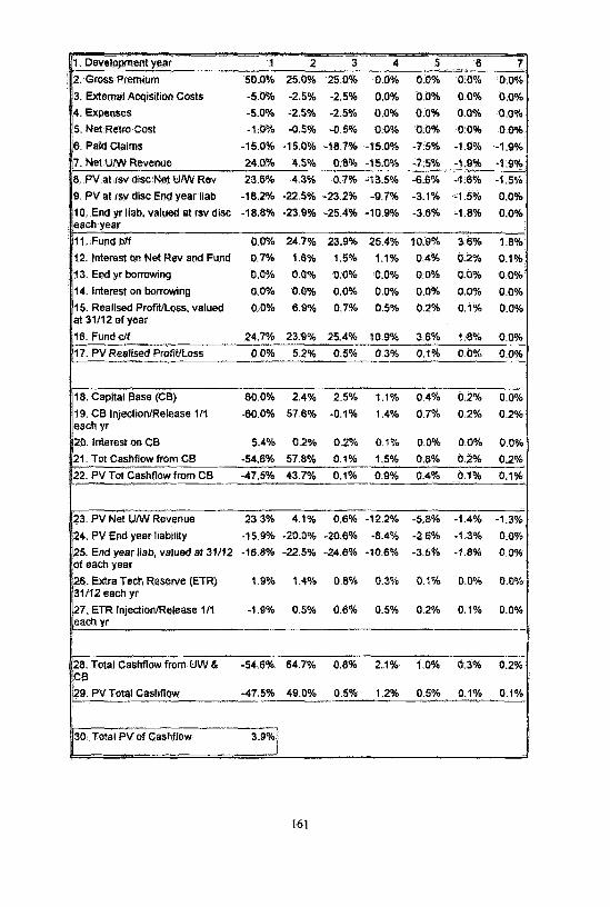
5. Net Retro Cost

End year

21. Tot Cashflow from CB -54.6% 57.8% 0.1% 1.5% 0.8% 0.2% 0.2%

22. PV Tot Cashflow from CB -47.5% 43.7% 0.1% 0.9% 0.4% 0.1% 0.1%

23. PV Net U/W Revenue 23.3% 4.1% 0.6% -12.2% -5.8% -1.4% -1.3%

24. PV End year liability

25 . of each year

26. Extra Tech Reserve (ETR) 31/12 each yr

28. Total Cashflow from UW & -54.6% 64.7% 0.8% 2.1% 1.0% 0.3% 0.2% CB

1. Development year 1 2 3 4 5 6 7

2. Gross Premium 50.0% 25.0% 25.0% 0.0% 0.0% 0.0% 0.0%

3. External Acqisition Costs -5.0% -2.05% -2.0% 0.0% 0.0% 0.0% 0.0% 4. Expenses -5.0% -2.5% -2.5% 0.0% 0.0% 0.0% 0.0%

-1.0% -0.5% -0.5% 0.0% 0.0% 0.0% 0.0%

6. Paid Claims -15.0% -15.0% -18.7% -15.0% -7.5% -1.9% -1.9%

7. Net U/W Revenue 24.0% 4.5% 0.8% -15.0% -7.5% -1.9% -1.9%

8. PV at rsv disc Net U/W Rev 23.6% 4.3% 0.7% -13.5% -6.6% -1.6% -1.5%

9. PV at rsv disc End year liab -18.2% -22.5% -23.2% -9.7% -3.1% -1.5%

10. End yr liab, valued at rsv disc -18.8% -23.9% -25.4% -10.9% -3.6% -1.8% 0.0%

0.0%

each Year

11. Fund Text b/f 0.0% 24.7% 23.9% 25.4% 10.9% 3.6% 1.8%

12. tnterest on Net Rev and Fund 0.7% 1.6% 1.5% 1.1% 0.4% 0.2% 0.1%

13. End yr burrowing 0.0% 0.0% 0.0% 0.0% 0.0% 0.0% 0.0%

14. Interest on borrowing 0.0% 0.0% 0.0% 0.0% 0.0% 0.0% 0.0%

15. Realised Profit/Loss, valued 0.0% 6.9% 0.7% 0.5% 0.2% 0.1% 0.0% at 31/12 of year

16. Fund off 24.7% 23.9% 25.4% 10.9% 3.6% 1.8% 0.0%

17. PV Realised Profit/Loss 0.0% 5.2% 0.5% 0.3% 0.1% 0.0% 0.0%

18. Capital Base (CB)

19. CB Injection/Release 1/1 each yr

20. Interest on CB

60.0% 2.4% 2.5% 1.1% 0.4% 0.2% 0.0%

-60.0% 57.6% -0.1% 1.4% 0.7% 0.2% 0.2%

5.4% 0.2% 0.2% 0.1% 0.0% 0.0% 0.0%

-15.9% -20.0% -20.6% -8.4% -2.6% -1.3% 0.0%

liab, valued at 31/12 -16.8% -22.5% -24.0% -10.6% -3.5% -1.8% 0.0%

1.4% 0.8% 0.3% 0.1% 0.0% 0.0%

Injection/Release 1/1 -1.9% 0.5% 0.6% 0.5% 0.2% 0.1% 0.0% 27. ETR each yr

29. PV Total Cashflow -47.5% 49.0% 0.5%

30. Total PV of Cashflow 3.9%

161

1.9%

0.1% 0.1% 0.5% 1.2%

However, the underwriting cashflow, resulting in a net underwriting revenue, cannot

simply be revalued at the same rate of interest as profits, as premiums are not available

for writing new business against until the corresponding claims have been paid.

Instead, they are put in a technical reserve, which is typically allowed to grow only at a

lower, less risky interest rate, often close to the long bond yield of the currency of the

book considered.

In many cases, regulatory concerns or company policy decisions prevents the reinsurer

from using even a risk-free rate for the discounting of the technical reserves, and a very

conservative rate is used instead, or no discounting at all takes place. The discounting

interest for the technical reserves in the example is 3%.

There are several interesting issues arising from the choice of interest rate on technical

reserves, most of which are beyond the scope of this paper. However, it deserves to be

mentioned that many companies with technical reserves predominantly invested in

equities, would still choose to use a low risk/risk-free, notional, discounting interest

rate, This is logical as long as the performance is measured against the risk-weighted

capital allocated to the insurance operations, as the insurance result on capital should

not gain from profits produced by taking investment risks, as long as these are backed

up by a capital base of their own. A company that would choose a higher interest

based on equity investments would thus also have to increase the capital base and/or

the return requirement. In our example profit test, we have chosen a nominal interest

rate on technical reserves of 6%. Investment expenses are assumed to have been taken

into account into this choice.

The final aspect of interest rates we need to bring up is the case where the cashflow

generated by the business does not generate enough funds for the technical reserves.

This is often the case for undiscounted reserves for long-tailed business. The required

funds can in principle be obtained by borrowing From shareholders capital, or from a

third party. The appropriate borrowing yield to apply depends on

1. The risk involved that the borrowed money may have to be used for paying

claims. If money is borrowed for a short-tail business being funded for three

years for accounting purposes only, this risk is very low, while if the money is

for long-tail business being discounted at a slightly conservative rate, the risk is

obviously considerably higher.

162

2. Whether the shareholders capital is seen as an indivisible entity, and an

risk-adjusted rate of return has been determined for this capital base, or if

different parts of the capital base are seen as being exposed to different levels

of risk.

In the example profit test, a borrowing yield of 10% is used.

The calculation of the table is straightforward, but in order to ensure a full

understanding for the discussion of the underwriting cashflow items in the next section,

we just briefly mention that

- PV End year liability, is the sum of all future PV Net U/W Revenues,

- The End year liability, valued at 31/12 of each year, is the preceding PV End year

liability revalued to 31/12 of each year by the technical reserve interest rate,

- Total borrowing, which is the technical reserve minus the available fund, and

- The interest rate on Net Revenue and Fund, is calculated as the interest for a full

year on the fund b/f and interest on 6 months on the Net U/W Revenue for each

year.

4.4.3 Underwriting Cash Flow Items

The items in the table has, somewhat artificially, been grouped into underwriting items,

lines 1 to 17, and capital base (CB) and extra technical reserve (ETR) items, lines 25 to

27. The present section will discuss the items normally directly connected to

underwriting, while the details of the CB and ETR’s are left for section 2.3.4. It is not

unusual to see profit test tables in the London market only covering the underwriting

cashflow, and this can to some extent be motivated by the typically quite small effects

of the other cashflows. However, for a full understanding of the results of writing

reinsurance business they should not be omitted. An additional reason for including

them would be, again, that the margins in reinsurance over time are not large enough

to ignore even small effects if their effects are negative, which is often the case for the

CB and ETR cashflows.

The premiums and claims paid distributions over time must be studied carefully in

advance, to determine an underlying development pattern (accumulated proportion

paid of ultimate by development year) for each one of them, and a forecasted ultimate

163

claims ratio. The payment patterns can be calculated from classical triangulation

schemes, with proper care taken to reflect expected future changes in payment speeds.

These triangles reflecting historic results also give ideas for future expected loss ratios,

which must be complemented with underwriting information.

For the table 1 profit test, the underlying development patterns are shown in the

following table:

Claims payment pattern

Ultimate loss ratio

20.0% 40.0% 65.0% 85.0% 95.0% 97.5% 100.0%

75.0%

Table 2. Payment patterns

Premiums and external acquisition costs are typically the most straightforward items.

However, in reinsurance, there are complicating features that make even them

stochastic. Firstly, the net premium may be determined by a claims-dependent formula,

such as a sliding commission, profit commission, a sliding scale or a reinstatement

premium and secondly, the reinsurance premium will always depend on the original

gross net premium income, which is only estimated in advance by the cedant. These

features will be reflected in triangulations for prior years only as long as the nature of

the business is not expected to change much in the near future.

Retrocession costs have to be modelled carefully, if retrocession is not bought only to

a negligible degree. As the profit table is concerned with expected cashflows, the net

retrocession cost after taking expected recoveries into account, should be given a

payment pattern. This pattern will greatly depend on whether the cover bought is

proportional or nonproportional. Again, triangulation schemes may be valuable,

although the losses to retrocession programmes are typically rare, so triangles would

often have to be coupled with sound judgement. A common simplification is to assume

that if very high-level covers are bought, the recoveries are so remote they can be

ignored, and then the retrocession payment premium is just a proportion of the

164

Development year 1 2 3 4 5 6 7

%

Premium payment pattern 50.0% 75.0% 100.0% 100.0% 100.0% 10.0% 100.0%

incoming premium. This is the simplifying assumption in table 1, where retrocession

costs have been set to 2% of the incoming premium.

It is also common to start the profit test table with the premium net after retrocession,

which is particularly suitable if the underlying triangulations are done on a net basis, or

if the retrocession is proportional.

The expense ratio is determined by the allocation basis and the overall expense level of

the company. A traditional approach would be to allocate expenses by premium

income, maybe modified for proportional/nonproportional and/or fac/treaty, depending

on the reinsurer’s organisation. A more detailed allocation can certainly be of value for

strategic purposes, for instance favouring growth areas,

Paid claims is the most obviously stochastic item in the table. The shown values are

expected values, but both the timing and the amounts are stochastic. Variability in final

loss ratio can often be calculated by modifying classical pricing formulae. Timing

variability has been studied very little in the actuarial literature, although some

guidance can be found in for instance in [Mack94]. If one is able to measure the

variability, a stochastic model in a simulation package could be set up to give a better

picture of the potential expected profits and timings. An example of this is shown in

section 4.4.8.

Underwriting profits or losses in this example are booked after two years, with

additional profits appearing with the unwinding of the discount. Other common rules

are realisation after one year, but with more conservative technical reserves, or

realisation spread out over several years. Both rules are easily implemented in the

profit test table. The decreased risk of taking out the profits later is matched by the

fact that their present value decreases with time, as the profits only earn a low return

as long as it resides in the technical reserves, while they are eventually discounted at

the return on investment requirement when released.

165

4.4.4 Capital Base Cashflow and Reserving Strain

A capital base is allocated to your business when the business is written, and then

released as the reserve is run off. The way in which the capital is allocated is

determined is not the subject of this section, and often the capital is released after one

calendar year, as a simplification. A tentative capital base, with a 60% capital to

premium ratio for the first year, and then a 10% capital to liability ratio for the

remaining years, is used to the profit test of table 1.

As the capital also produces investment income, this interest needs to be included in

the model. The investment policy for the capital base may differ substantially from the

policy for technical reserves, as it is often less conservative and contains a higher

proportion shares, so care must be taken to reflect that properly. As already discussed

in section 4.4.2, a common approach is to include only a nominal growth on the capital

base, and consequently keep the risk-weighted target return free from investment risk,

although this is by no means the only way to proceed.

One may think that adding the investment income from the capital base may

automatically give a higher profit in the profit test, as more income but no new losses

are added. However, the required return from underwriting and capital growth is

naturally higher than that from underwriting alone. This is reflected in the

risk-weighted target return at which the profits are revalued, which now is the

company’s full return on investment requirement and in the target profit, so it does not

necessarily lead to easier targets. The present value profits at varying target returns as

shown in graph 1 for the example profit test at a constant ratio.

166

Graph I PVReturn on Capital as a

function of the target ratio

Graph 2 Pv ROC sensitivity to

ultimate loss ratio

Thus, we need three lines in the profit test to conveniently describe the effect of the

capital base, one for the capital base itself, one for the necessary injection or release of

capital to shareholders, and finally one for the nominal interest on the capital base,

To be able to run off our capital base against the technical reserve and to compute

interest rates on reserves, we need to know exactly how the reserves are determined.

This information could be in the form of an IBNR profile, a reserve discounting policy

and a general reserving policy (degree of conservatism, “50/50” reserve etc.). An

IBNR profile giving more prudent reserves than the present value of future liabilities, a

policy to discount technical reserves at a low interest rate, a general policy to carry 5%

more reserves than the expected loss or reserves enough to meet liabilities with a high

probability, are all different ways of specifying the extra reserve, which is really just a

way to increase the capital base allocated to the line.

In the example profit test, we have as already mentioned used a conservative interest

rate for technical reserves as this is the most common way of specifying an ETR, but

then we have also calculated the amount by which the reserve is prudent, as this

information shows the increase in the actual capital base.

167

If the introduction of an ETR is for accounting or regulatory purposes, the pattern of

emerging profits is more often than not affected. The “unwinding of the discount" is

probably the most common example of this. However, if the ETR is a provision against

run-off deviations, one could just as well argue that the profits could be realised just as

without this extra reserve.

Taking the present value of the injections and releases of capital base amounts gives us

an amount to be added to the present value of the underwriting cashflow , giving us

the NPV of the business segment considered in the profit test. This value can then, for

instance, be divided by the capital base of the first year, giving a return on capital

measure. If this value meets the target one, then the studied segment of business is

considered sufficiently profitable to take on the books, or to continue to write.

Naturally, the target return may have been set to reflect a long term commitment to a

territory or class (it may even be negative!), and therefore meeting the target does not

necessarily mean profitability.

In another approach we would set the investment return, return on equity parameters

and also the target profit according to our assumptions and requirements and

subsequently solve for the highest L/R allowing us to meet the target. This approach

has its value in that it provides the underwriters with a parameter that is meaningful to

their work, and can be discussed with cedants.

There are several other ways to use the results of the profit test. A common method

from the life insurance industry would be to actually solve the entire table for the rate

of return (the internal rate of return, IRR) giving a nil present value of the total

cashflow and compare this to the target rate of return. As Gpraph 1 shows the ROC as a

function of the target rate, the IRR can be looked up immediately from the graph. In

general business, the total cashflow can in fact change sign more than once, giving rise

to the well-known problem of multiple IRR’s. We will see two more profit test

applications in sections 4.4.6-8.

The sensitivity of profit to small changes in the ultimate loss ratio is typically quite

high, and this is depicted in Graph 2. A capital to premium ratio of 60% is assumed for

this class. It is worth pointing out though, that the effect often is roughly linear, as long

as profits are realised within a few years.

168

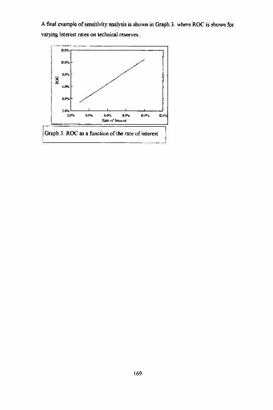
A final example of sensitivity analysis is shown in Graph 3. where ROC is shown for varying interest rates on technical reserves..

Graph 3. ROC as a function of the rate of interest

169

4.4.5 The Application of Profit Tests at Different Levels of Aggregation

In the preceding sections, we have looked at a generic profit test, without reference to

any difference in application depending on the level at which it is applied or to the

relative importance of different problems. In this section, we aim to give some

guidance on these issues.

There are three obvious levels of application,

1. the whole account level,

2. the business segment level, and

3. the individual treaty level,

The most common application would be the second one, where many of the

parameters are already set, for example capital allocation, retrocession and

management expenses, and the typical question is whether a certain book of business is

profitable or not, or at what target loss ratio it could be written to be profitable. The

business segment needs to be a reasonably homogeneous for the profit test to be valid,

as a mix of long and short tailed business could distort the effects of investment

income.

In order to answer some of the strategic issues arising a whole account level, for

example about optimal premium volumes and suitable expense and capital allocations,

the profit test needs to be applied to the whole account. This does not mean just one

profit test for all business, especially in view of what has just been said about

homogeneity, but rather a number of simultaneous profit tests, run with different

scenarios for the studied strategic parameters. In life insurance terminology, this would

be a “model office”. This is an integral part of the planning process. The practical

problems of actually carrying out an optimisation in this environment are enormous, so

one would typically have to confine oneself to look at a small number of scenarios,

Another issue to consider when using profit tests for strategic purposes, and in

particular for multiyear planning, is the issue of tax. If the target ROC is set net of tax,

one has to bear that in mind in the profit calculation. In particular, if the target ROC is

considered a long-term average target, and if results are volatile, tax will only be paid

on profitable years, and hence simulations or scenarios are necessary, rather than just a

straight percentage deduction,

170

Finally, when most parameters have been set in the cascade structure of the whole

account and business segment profit tests, we need to perform profit tests for

individual treaties, or groups of treaties. Overall targets without proper reference to

individual circumstances, or at least territory and class-specific calculations, are seldom

accurate enough. Obviously, it is difficult to determine payment patterns for single

treaties unless very large, but as far as possible one must try to use similar treaties and

to reflect present, not past, market conditions and practices.

4.4.6 Application 1: Distribution of Portfolio Results through Simulations

In this section, we look at the variability in results for a nonproportional, long-tailed

line of business, and the effects of uncertainties in some of the underwriting

parameters.

The portfolio studied is a book of liability business, where the loss ratio for a specific

underwriting year has been estimated to be normally distributed, for simplicity, with an

average of 95% and a standard deviationof 10%. The premiums are paid up-front, and

the claims are paid with a linear payment pattern over 10 years. Brokerage is 10%,

internal expenses 10%, capital base 50%, and the rest of the parameters are as in our

example profit test from section 4.42. As the result sensitivy to variations in the loss

ratio is roughly linear (cf. graph 2), the return on capital (ROC) distribution is

approximately normal as well, as shown in graph 5. The expected value and standard

deviation are 3.1% and 6.9%. The expected value can be compared to the

deterministic profit of 3.5%. 1000 simulations in @RISK were run.

I71

Ap

Graph 5. Distributions of results with deterministic and stochastic payment delays.

The next step in our study is to look at the sensitivity to payment delays. What if we have got

the average payment delay (5 years) wrong? First of all, let us just look at the

deterministic result after changing the pattern to a linear one with a 5.5 year average.

The ROC now becomes 6.5%, which is quite a large difference, considering that the

future average payment delay is often hard to determine with good precision. If we, for

the sake of argument, consider the payment delay to be an uncertain, random variable,

with say a uniform distribution between 4.5 and 5.5 years, and run the same

simulations as above, the standard deviation now becomes 7.9%, while the expected

value is 7.0%. The explanation for this is of course that we add uncertainty in the

payment pattern, but the since the effect is roughly linear for a small change in the

payment delay, the expected value does not change.

Finally, we are going to try to take into account that this particular book’s ultimate loss

ratio is sensitive to the average payment delay through social inflation. If we make the

simplified assumption that the expected loss ratio goes from 90% to 100% as the

average payment delay goes from 4.5 to 5.5 years, due to social inflation on this

nonproportional account, we can very easily build this into our simulation model. The

standard deviation for the loss ratio is now reduced to 4.0%. The ROC distribution for

172

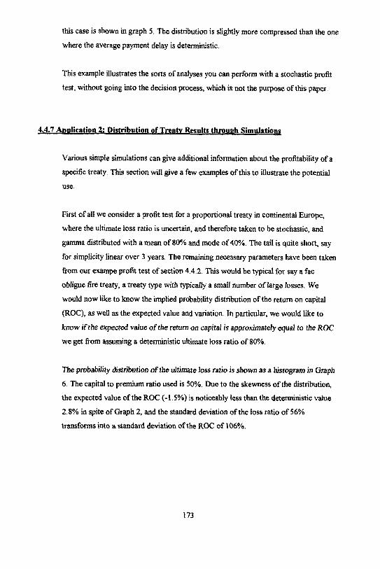
this case is shown in graph 5. The distribution is slightly more compressed than the one

where the average payment delay is deterministic.

This example illustrates the sorts of analyses you can perform with a stochastic profit

test, without going into the decision process, which is not the purpose of this paper.

4.4.7 Application 2: Distribution of Treaty Results through Simulations

Various simple simulations can give additional information about the profitability of a

specific treaty. This section will give a few examples of this to illustrate the potential

use.

First of all we consider a profit test for a proportional treaty in continental Europe,

where the ultimate loss ratio is uncertain, and therefore taken to be stochastic, and

gamma distributed with a mean of 80% and mode of 40%. The tail is quite short, say

for simplicity linear over 3 years. The remaining necessary parameters have been taken

from our exampe profit test of section 4.4.2. This would be typical for say a fac

obligue fire treaty, a treaty type with typically a small number of large losses. We

would now like to know the implied probability distribution of the return on capital

(ROC), as well as the expected value and variation. In particular, we would like to

know if the expected value of the return on capital is approximately equal to the ROC

we get from assuming a deterministic ultimate loss ratio of 80%.

The probability distribution of the ulimate loss ratio is shown as a histogram in Graph

6. The capital to premium ratio used is 50% . Due to the skewness of the distribution,

the expected value of the ROC (-1.5%) is noticeably less than the deterministic value

2.8% in spite of Graph 2, and the standard deviation of the less ratio of 56%

transforms into a standard deviation of the ROC of 106%.

173

Graph 6. Gamma distributed claims ratios.

A more interesting question could be the following: What if the commission is a sliding

commission going from 20% to 0% for loss ratios from 60% to 80%? Is the expected

commission still 10/o? What is the expected ROC?

The distribution of commissions and ROC is shown in a pair of histograms below,

Graphs 7&S, the expected commission is 12.0%, which is a not insignificant deviation

from the deterministic 10%, and consequently the ROC has lost value to -5.5%. The

standard deviation is reduced significantly, which is the very purpose of the sliding

scale commission, to 86%.

The questions posed above were just intended for illustration purposes, and were by no

means chosen for radical results. There is a multitude of questions to be asked for each

treaty of segment of business in questions, and in many cases the answers can be quite

surprising, both in terms of giving different expected values than expected, but also by

the large variability in the results.

174

Graphs 7&8

Distributions for sliding scale commission and ROC, given a gamma distributed

4.4.8 Application 3: Optimisation of Portfolio Mix

An important application of profit tests is the area of strategic planning for business

units writing a more than one line of business. This would be part of the planning

process and we are here looking at a one-year planning horison only. The actual profit

test is an integral part of the optimisation procedure, and will become important if at

least one of the lines of business is a long-tailed one. We will look at a simplified, but

non-trivial example of determining the optimal business mix for a book of two lines of

business, catastrophe excess of loss, which is very short-tailed, and nonproportional

motor third party, which is very long-tailed. To fix ideas, let us assume that the

business is written in the UK. For each line, the profits, capita1 needed and costs will

be described, and subsequently the optimisation procedure and results are presented.

The company in question deem it possible to write between 10 and 20 million pounds

cat x/l for the year in question, the management expense ratio depends on the income

written. There are both fixed and variable costs, and the total expense ratio can be

described as

175

where p is the cat x/l income in millions of pounds. As almost no diversification is c

achieved by writing more income for this class on its own, all ceding companies are

likely to be hit rougly to the same degree by a windstorm or flood, the capital base is

decided to be 120%, irrespective of income level. The underwriter also estimates that

the expected L/R at which he would write the book at would increase from 50% to

60% linearly as the income rose. Acquisition costs are 10%.

For the motor book, the feasible income range is estimated to between 10 and 30

million pounds and the expense ratio

where p is the motor income in million pounds. m

As the treaties are relatively independent, and as most potential treaty shares would be

roughly of the same size, it is estimated that a capital base (expressed as a percentage

of premium)

is adequate for the class written on its own. Thus, at minimum income level, the capital

base would be 63%, and at maximum level, it would be 37%. For this portfolio, the

L/R estimate From the underwriter is that the L/R will increase from 100% to 120%

with income, and acquisition costs are 10%.

The capital base advantage of writing the two classes together is felt to be

appropriately reflected in a reduction of the overall capital base percentage by the term

(“covariance term”)

r = 0.4c c c m

This formula could have been arrived at by way of stochastic modelling the

portfolio. The resulting overall capital need is shown in a graph for two different levels

of catastrophe business and a range of levels of motor business.

176

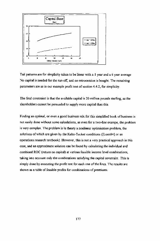
Tail patterns are for simplicity taken to be linear with a 1 year and a 6 year average.

No capital is needed for the run-off, and no retrocession is bought. The remaining

parameters are as in our example profit test of section 4.4.2, for simplicity.

The final constraint is that the available capital is 20 million pounds sterling, as the

shareholders cannot be persuaded to supply more capital than this.

Finding an optimal, or even a good business mix for this simplified book of business is

not easily done without some calculations, as even for a two-line exampe, the problem

is very complex. The problem is in theory a nonlinear optimisation problem, the

solutions of which are given by the Kuhn-Tucker conditions ([Luen84] or an

operations research textbook). However, this is not a very practical approach in this

case, and an approximate solution can be found by calculating the individual and

combined ROC (return on capital) at various feasible income level combinations,

taking into account only the combinations satisfying the capital constraint. This is

simply done by executing the profit test for each one of the lines. The results are

shown as a table of feasible profits for combinations of premiums.

177

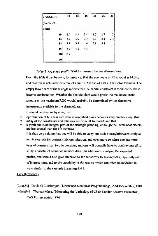
Cat\Motor

Premium

(£m)

10 2.9 3.3 3.4 3.2 2.7 2

12 3.2 3.6 3.7 3.6 3.1 2.4 14 3.4 39 4 3.9 3.4

16 3.6 4.1 4.3

18 3.7

20

Table 2. Expected profits (£m) for various income distributions.

From the table it can be seen, for instance, that the maximum profit amount is £4.3m,

and that this is achieved for a mix of about £16m cat x/1 and £18m motor business. The

empty lower part of the triangle reflects that the capital constraint is violated for these

income combinations, Whether the shareholders would prefer the maximum profit

amount or the maximum ROC would probably be determined by the alternative

investments available to the shareholders.

It should be obvious by now, that

optimisation of business mix even in simplified cases becomes very cumbersome, that many of the constraints and relations are difficult to model, and that a profit test is an integral part of the strategic planning, although the investment effects are less crucial than for life business,

It is thus very seldom that one will be able to carry out such a straightforward study as

in this example for business mix optimisation, and even more so when one has more

lines of business than two to consider, and one will normally have to confine oneself to

study a handful of scenarios in more detail. In addition to studying the expected

profits, one should also give attention to the sensitivity to assumptions, especially rate

of interest ones, and to the variability in the results, which can often be modelled in

ways similar to the example in section 4.4.6.

4.4.9 References

[Luen84] David G Luenberger, “Linear and Nonlinear Programming”, Addison-Wesley, 1984

[Mack94] Thomas Mack, “Measuring the Variability of Chain Ladder Reserve Estimates”,

CAS Forum Spring 1994.

178

10 14 18 22 26 30

u

u

u

4.5 UNDERWRITING MANAGEMENT

This section describes the problems encountered in managing the underwriting cycle

and possible approaches to overcoming the problems. The section covers topics such

as determining the underwriting targets, balancing the portfolio of business and

individual risk selection.

4.5.1. Managing the Underwriting Cycle

It could be argued that how can one manage the underwriting cycle if it can not be

measured or predicted. Furthermore, if the cycles were predictable, then people would

act accordingly, and make the cycles unpredictable.

What we get is extremes of cycles, The cycles are caused by actual underwriting

experience and perception of how that experience is expected to develop over the next

few years. As a result of adverse claims experience the capacity for writing new

business diminishes putting upward pressure on rates. Then the ensuing hard market

leads to a period of profitability attracting new capital and capacity to the market

which in turn put downward pressure on the rates. The extent of rigidities in the ability

to increase rates or attract new capital affects the degree to which the cycles are

extended and accentuated.

As for predicting the cycles, the reinsurance cycles may precede the insurance cycles.

The extent of the availability and cost of reinsurance may affect the rates insurers can

charge the primary insureds. Conversely, the demand for insurance may be affected by

the economic climate. Thus, the supply and demand for reinsurance is very difficult to

forecast.

Therefore, managing the underwriting cycle may be less concerned with forecasting

the cycles accurately, and more concerned with the ability of the company to respond

flexibly, speedily and profitably to an eventuality falling within a reasonably acceptable

range of scenarios.

179

In order to achieve this, the company may consider the likely economic climate and

market trends over the foreseeable future and take a view about a range of expected

market conditions, It is possible that different conditions may be expected for different

segments of the market ( e.g. by class of business or territories). The company would

then consider a range of business strategies appropriate to the range of expected

scenarios.

A detailed audit of the company’s resources and capabilities will enable the company to

identify any needs in terms of capital or resources to adopt a given strategy and to be

in a position to respond to changes in market conditions.

Thus, managing the underwriting cycle is about being in a state of preparedness to

respond to a given change in market conditions within an expected range of scenarios.

The extent of analysis carried out internally and externally, and the flexibility of the

organisation structure to respond to a given change would differentiate between the

companies which are able to survive and prosper in the current competitive climate of

global reinsurance and the companies which are not.

4.5.2 Underwriting Targets

The underwriting targets may be discussed and agreed when the corporate plan is

prepared. The targets may be broad in terms of premium income, target loss ratios,

and target operational ratios for the business units, or they may be more detailed in

terms of units of risks within a class of business in a given territory.

The targets may be constrained by fimits on aggregate exposures which may be

determined in the light of the company’s outwards reinsurance program. There may

also be limits on risk size for an individual risk, groups of risks, or exposure to a given

reinsured.

The underwriter will want to ensure that he makes full use of the available capacity to

achieve not only his immediate targets but also to develop long term relationships with

the reinsured for mutual benefit. He will want to ensure that adequate returns are

made in relation to the risks accepted without penalising the reinsured for an

exceptional bad experience.

The underwriter will have an understanding of the portfolio of business he has written

in terms of the risk profile of the business. He will perform an analysis of the portfolio

180

by the number of risks and program of risks with a given reinsured and how that

program has behaved over the past and is continuing to behave. Such portfolio analysis

may be carried out periodically at a detailed level to identify the significant risk

exposures, The underwriter will also consider the cost and benefit of such analysis in

relation to future profitability,

The detailed portfolio analysis at periodic points will enable the underwriter to

consider the current shape of the portfolio and the desired shape of the portfolio in

order to meet his underwriting targets. In this context, he may consider the current

security rating of the reinsured in order to take a view as to continued existence of the

reinsured in the foreseeable future. The underwriter will be effectively building a

portfolio which is expected to be durable and profitable over the longer period.

4.5.3 Balancing a Portfolio

It is a fundamental concept of insurance business to spread the insurance risk over a

large portfolio of insureds to obtain some stability and predictability to the emerging

losses. It is therefore important to ensure that any insurance operation has a large and

diversified portfolio of risks both within class and over the whole company. Against

this is the constraint that the number of such risks need to be correctly underwritten

and managed.

The underwriting targets at the corporate plan level will attempt to balance the

portfolio at the highest level to achieve a desired risk/reward trade off. At a business

class level, a portfolio analysis will highlight the current risk profile and the desired risk

profile in the future. In this context, the underwriter will be concerned with benefit of

diversification compared to the potential cost of diversification from additional

resources required to service that portfolio, Conversely, a fewer number of risks well

researched and costed may well generate less volatility.

The risk profile and the balance of a portfolio could be investigated by formulation of a

model office for the classes of business which are currently being written. The model

office will include specimen policies representative of the portfolio and can attempt to

simulate losses for those policies on a range of assumptions. The model can be

expanded to incorporate various assumptions associated with the insurance operation

The effect of changing the risk profile on the stability can be investigated. A balanced

181

portfolio is one where the aggregate expected losses are stable over time and do not

demonstrate large volatility

The concept of the model office can in fact be significantly expanded to model the

company as a whole, In this case all the constituents such as premiums, assets,

expenses, investment returns can be incorporated within the model office. The model

office would then consider the volatility of the emerging profits on current conditions

and perform various scenario testing to determine the effect on profitability and the

solvency position on different sets of assumptions,

4.5.4 Risk Selection

In selecting an individual risk the underwriter may use techniques such as those

described in this paper but ultimately he will exercise underwriting judgement on

whether the risk contributes towards his overall underwriting targets.

The underwriter will be constrained by what risks are presented to him. This will

depend on his standing in the market and the perception of his company’s image and

security rating. If the underwriter is considered a lead underwriter, then his past

performance may well be under regular scrutiny. In order for a program to be fully

subscribed by the market, the lead underwriter’s rating has to be respected and

acceptable to the following underwriters.

The underwriter will select an individual risk not only because it is technically priced

adequately, but also whether it falls within his general underwriting strategy and

underwriting authority. Typical considerations are:-

1 The limits of liability.

2. Any potential impact on the outwards reinsurance treaty.

3. The Annual Premium Income Limits set by his Board.

4. The minimum premium limits per risk

5. The minimum rate on line.

The underwriter will also be looking to develop and maintain a long term relationship

with the reinsured. In any business, it is more expensive to generate new business than

to renew existing business. The underwriter will therefore wish to select those

reinsureds who are likely to be profitable, show good risk management skills and are

expected to survive the peaks and troughs of underwriting cycles.

182

aae will consider the group of policies with a given reinsured to ensure

that the overall returns from these policies are adequate. He will also want to ensure

that he makes good use of his capacity to write catastrophe business by leveraging this

against other classes of business relating to the reinsured. There are other

considerations,

1. Exclusivity of risk

The underwriter may exercise commercial judgement when considering certain risks.

For example, he may take a higher percentage line with the intention of keep the risk

exclusive. A 100% line may be written with the intention of preventing competitors

having access to the risk. Writing at a 75% level will open the door to other insurers

and could readily result in the signing down of the risk, as well as a potential loss of

information,

2. New line of business.

When presented with a new or unusual line of business, the underwriter may initially

accept a small line in order to gather the underlying experience before fully committing

himself,,

3. High Profile Risks

The underwriter may also at times take on a high profile risk for reasons of prestige.

4. Cross subsidy within a risk

An underwriter may accept a lower rate for a particular layer to access a more

attractively priced layer in the same program. In this case it is the overall combines

profit that is important.

Finally, underwriting should be considered as much as an art as science. it is important

to ensure that all the technical aspects are fully explored and correctly costed.

However, ultimately the skills of underwriting may be in understanding in depth

qualitative information relating to the nature of an individual risk and the quality of

reinsured, as well as in negotiating the best price for the risk.

183

underwriter

5. The Role of Actuaries in Pricing

5.1 This paper has broached the subject of Actuaries becoming more involved with the

underwriting process. This naturally prompts the question “Would involving actuaries

in the underwriting process be of benefit to the business?” There are clearly mixed

reactions to this type of proposal as some may view this as be taking over the

underwriting role. Qualified actuaries have even progressed to underwriting lines of

business both in U.S. and in Europe.

5.2 When we started to write this paper, the actuarial role in most London Market

Companies was essentially one of reserving, and only occasionally were they asked for

their opinion on rating. These risks tended to be those with a large volume of historic

loss data which requires techniques similar to reserving to project the profitability of

these past years. During the ensuing months there was a clear trend to actuaries being

employed in a pricing role, particularly in those companies with European or American

parents.

5.3 The skills of the actuary and underwriter are complementary. The actuary has

considerable technical skills, and in this respect he is better equipped than the

underwriter. This paper has dealt with those skills by illustrating the calculation of the

technical rate for the risk. Having computed this rate, the underwriter imputes his skills

which takes into account market conditions, handling negotiations with brokers, and so

on. The skills required in the underwriting process are:-

1. Risk selection and assessment

2. Product design (coverage, terms and conditions)

3 Treaty wording and legal skills

4. Contract negotiation with cedant or broker

5. Questions of balance of portfolio

6. Longer term strategy.

We have shown that actuarial skills could assist in the management of this process,

particularly in the first and last two area.

184

5.4 The crucial point is that underwriters must first have confidence in the actuary. For this

condition to hold actuaries certainly need to understand the underlying business and

have a working knowledge of the various contracts. This extends to the standard

policy wording and the slip details and market conditions

5.5 Factors affecting the future exposure change. The risk management features of the

account needs to be understood for the actuary to translate from the historic loss

experience (and any collateral data employed in the rating) to the new exposure period

being assessed. Experience in this process could be gamed by the actuary spending a

portion of his training period in the underwriting room assisting in the day to day

underwriting. The average period to qualify for a good student actuary is between 4 to

7 years, so a period of 1 to 2 years in that function is not unrealistic.

56 One by product of this training strategy is that the student would be in a position to

add considerable value to the continuing reserving process of the account. The role of

the Chief Executive of a London Market operation is also as Chief Underwriter, and if

actuaries harbour ambitions to achieve such a status then it is essential that they have a

sound grasp of the day to day operations in the underwriting room and the difficulties

that underwriters have in pursuing their objective of writing profitable business. Can

actuaries achieve this goal while pursuing a purely reserving role.?

5.7 As actuaries become more involved in this role there is clear potential for a conflict

between a pricing and reserving role, not least in the remuneration is contingent on the

performance of a specific account. There is a clear need for professional guidance with

the possibility of divorcing the actuarial pricing and reserving roles. Such a divorce

between sales and control is extremely common in other financial service industries.

5.8 In conclusion, this paper illustrates the skills that have evolved and continue to be

developed as actuaries become more involved with the pricing role. These new skills

are becoming actively used in many companies; and will give companies who use

actuaries in pricing a distinct competitive advantage.

185

Appendix 1 More Advanced Techniques

The purpose of this appendix is to explore new techniques that may be applied to

London Market business or new approaches that are being developed. Some of these

techniques have been applied in the past, but are complex mathematically and esoteric

in places

These can be classified into three types of development.

1. Direct Modelling.

In section 3 we had mention of Generalised Linear Models. These type of models are

being slowly introduced into London Market rating. On top of these lie Fuzzy Sets and

NeuraI Networks. Fuzzy Sets apply when there is uncertainty about the choice of the

rating parameter. Neural Networks apply when there is uncertainty about the model.

Neural Networks are described in more depth in Appendix I.2

2. Modelling of Extreme Events,

The buzz words of the moment are Chaos Theory and Self Similarity. Some of the

Distributions generated by this theory give a better fit to both frequency and size of

some of the catastrophic events we have recently had than the more conventional

theories and distributions.

3. The use of Financial Mathematics to rate policies.

An Excess of LOSS Policy has the same pay off structure as an option so can’t we price

them in a similar way? The Return on Equity approach to pricing which is found in US

rating has its foundations in Financial Mathematics.

186

Appendix 1.2 Direct Modelling - Neural Networks.

Trying to model the underwriting process using a mathematical black box is not new.

In the early 1980’s the Government, ABI and a number of Insurance Companies tried

to create an expert system that would emulate the underwriting of UK Commercial

Business. The derived model was not used in practice. Ayling [ 18] undertook an

analysis of a London Market underwriter in the Aviation Excess of Loss Market He

attempted, by standard statistical methods, to identify and measure the components

used to rate such business. The results of the analysis indicated the task was extremely

difficult

1. Claims in the underwriting year could not be reasonably be assessed from slip details

at the beginning of the year.

2 Price variations over a period were being reasonably estimated

3. There was no strong relationship between premiums charged and the ensuing claim

costs.

4. The premiums charged by the underwriters could not be reasonably estimated from

details on the slip.

This work was done in 1984 on data then 10 years old, but is still a slightly

disconcerting. The years being reviewed were the profitable years!

One option to this problem is to use neural networks to try and understand what is

happening. There are currently a number of software houses selling neural network

systems. They tend to be black box in nature, but have the potential advantage in that

they can capture the essentials of what is happening in certain systems, particularly

those involving human behaviour, over the more traditional models. They act by

learning what the underwriter has done before to come up with an answer consistent

with recent proposals. To be a good system, it is important to have rejected contracts

in the data base, and this is often a barrier to practical application.

187

There are three types of systems that might be considered

System Type 1.

Under this type contract information is input, and the system decides whether the

contract is likely to be underwritten or not. Rejected policies are not processed full

System Type 2

Based on recent policies that have been underwritten, what is the likely premium I

for the contract under review.

System Type 3.

How much of the risk do I want to take.

Clearly non-neural network systems can be devised to solve these problems.

Input to Hidden Layer

Hidden to Output

f(x) a transfer function

h(j) = Sum (w(i,j)xI(i))

S(j) = f(h(j))

h(k) = Sum (W(j,k)xS(j))

o(k) = f(h(K))

I(i) are the network inputs

O(k) are the network outputs

W(i,j) represent the weight connecting neuron i in layer 1 to neuron j in layer 2

W(j,k) represent the weight connecting neuron j in layer 2 to neuron k in layer 3

f(x) is the neuron transfer function, for example 1/(l+exp(-x)).

188

This function is not dissimilar to the inverse link function in Generalised Linear

Models. However GLLM models are usually fitted by maximum likelihood methods,

neural networks are trained by least squares. Neural networks can model non linearity

189

Appendix 1.2 Chaos Theory and New Distributions

Alpha Stable Non Gaussian Distributions.In 19th Century mathematicians discovered that the best fit of a curve to a series ofpoints was achieved by the method of least squares, The distribution of errors

emphasised the importance of the Normal or Gaussian Distribution. At the same timeFourier invented his famous series and transforms and this was applied to probability

distributions to generate characteristic functions, Laplace noted that the the Gaussiandensity function was its own Fourier transform.In 1850 Cauchy extended this to generate further distributions

This essentially replaced the Fourier integral using t withtN

When N=2 we have the Gaussian caseWhen N=l we have the Cauchy Distribution

In 1919 Bersham showed-that fN was probability distribution if 0 <N _< 2.Traditionally N is replaced by aThese distributions have special features.1. The central limit theorem does not apply for < 22. They are stable in the sense that if X1,X2 are random variables with the same

distribution then CX = C1X1 + C2X2 has a similar distribution with the sameindeX foranyC,C1,C2when

These distributions have many interesting features, with high value radical jumps.Having said this the mathematics of emulating the process is difficult,

190

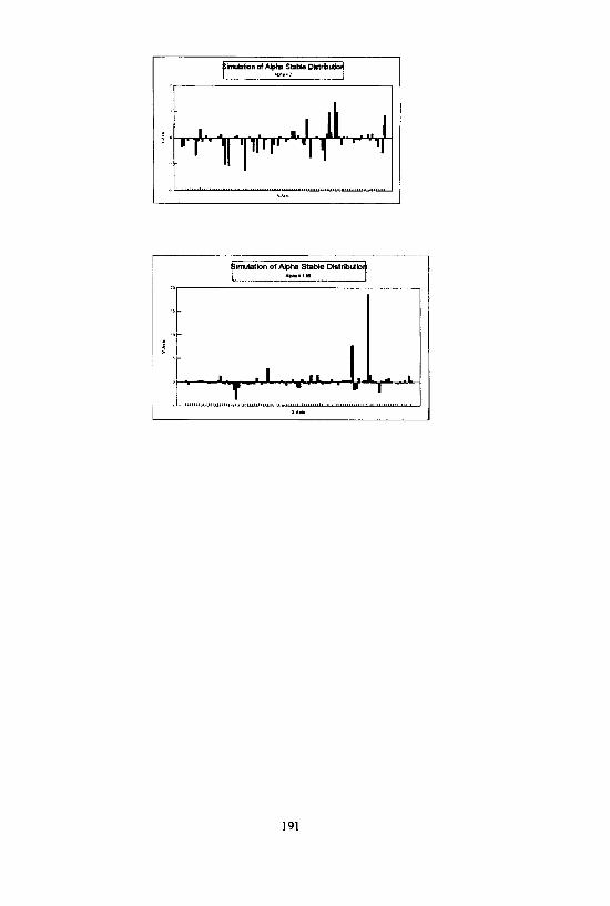
191

Appendix 1.3 Modelling of Extreme Events

For certain classes of reinsurance the modelling of extreme events is of paramount

importance. In modelling claims distributions it is often found that whereas the

distribution gives an excellent tit to the bulk of the data, the extrapolated tail

distribution may appear to differ significantly from what few data points that may exist.

In modelling extreme events then there are often few or even no data points in the

range where the quotation is required. This problem may be solved by the use of fitting

extreme curves,

The Fisher Tippet Theorem comes, in part, to the rescue. This states that data will

trend to one of three distributions, subject to an affine ( linear with positive slope)

transformation.LetThis gives rise to a class of distributions known as MAX-STABLE providing they

satisfy max(X1,. ..... ,Xn) cnX+dn,cn > 0

The Fisher-Tippet Theorem then statesLet Mn = max(X1,........ ,Xn) where {Xk} is a sequence of independent randomvariables.If, for some sequence of normalising constants, cn > 0,dn there exists anon-degenerate random variable Y such that

then the distribution of Y is one of the three following types.

Frechet

Weibull

Gumbel

if

Hence in the Frechet Casein the Weibull Casein the Gumbel Case

192

ififif

as

ExampleLet {Xk} be Cauchy, i.e.

As (by l’Hopita1)

The types of distributions are as follows

FRECHET Cauchy, Pareto, Loggamma, Burr, Benktander Type 1

WEIBULL Uniform, Polynomial Growth, Beta

GUMBEL Generalised Weibull, Exponential, Gamma, Normal;

Lognormal

The estimation of the parameters is undertaken using a variety of estimators, of which

the most useful is possibly the Hills estimators. The software package XTREMES,

which is associated with the book “The Law of Small Numbers: Extremes and Rare

Events” by Falk et al and published by Birkhausen concentrates on this approach. In

addition there are approaches known as Quick estimates and Mean Estimates.

Attached is an example and data set of Hurricane Data from Hogg & Klugman

This uses the Xtremes software and assumes different numbers of extreme points..

In addition a book entitled “Modelling of Extreme Events in Insurance” by Embrechts

et al is soon to be published by Springer. There is a bibliography of over 340

references.

Fitting of Hurricane Projections Using Hill Estimators

193

Hence

i.e. Frechet with

HURRICANE DATA

Total damage done by hurricane (in $1,000,000)

Source: Hogg R.V. and Klugman, S.A. (1984), Loss Distributions. Wiley, New York.

History: Total damages above $5,000,000 caused by hurricanes from 1949 to 1980

compiled by the American Insurance Association A trend factor is included which is

based on the Residential Construction Index.

Hogg R.V. and Klugman, S.A. (1984): Suggest, according to the empirical mean

residual life (excess) function, that the Weibull and lognormal distributions may

provide good models for these observations.

Data Set

5,6.766,7.123, 10.562, 14.474, 15.351, 16,983, 18.383, 19.030,25.304,29.112,

30.146,33.727,40.596,41.409,47.905,49.397,52.600,59.917,63.123, 77.809,

102.942, 103.217, 123.680, 140.136, 192.013, 198.446,227.338, 329.511,361.200,

421.680,513.586, 545.778,750.389,863.881, 1638.000.

194

Appendix1.4 Relativistic Methods- Options and Curves

One of the questions that can be raised is whether a contract has been priced well with

respect to other contracts in the same programme or with peer contracts in other

programmes. These have been viewed by two approaches, namely Option pricing

Theory and Curve Pitting techniques,

Option Pricing

In [ 20 ] Sanders noted the similarity between the pay off pattern of an option and a

stoptoss policy. The question was explored whether the theory of option prices could

assist in either the absolute or relative pricing of aggregate excess of loss contracts and

catastrophe excess of loss. In other words have the layers been priced consistently

The Black-Scholes formula, calculated in Option Price theory, makes assumptions of

lognormalilty in the incremental price jumps.

The formula isWhere

N(*)=cumulative normal distribution

This calculation is derived from Stochastic calculus, although an alternative approach

in the paper is to use a binomial model.

The equation is normally used to calculate the option price, and for this we need to

calculate the volatility The trick is to reverse the issues; for a given option price there

is an implied volatility.

In the paper Sanders used this approach to calculate the reinsurance cost based on the

assumed volatility of a particular portfolio, given specific quotes, and to simulate costs

when the claims distribution when not log normal There showed a remarkable

consistency between the results of the simulation and the pricing using the Black

Scholes equation on a stop loss model.

195

c = cost of a call

S = current price

T = timeE = exercise price

o2 = volatilityRf = risk free rate of interest

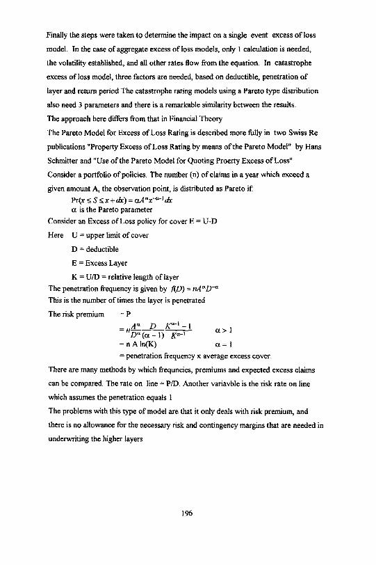
Finally the steps were taken to determine the impact on a single event excess of loss

model. in the case of aggregate excess of loss models, only 1 calculation is needed,

the volatility established, and all other rates flow from the equation. In catastrophe

excess of loss model, three factors are needed, based on deductible, penetration of

layer and return period The catastrophe rating models using a Pareto type distribution

also need 3 parameters and there is a remarkable similarity between the results.

The approach here differs from that in Financial Theory

The Pareto Model for Excess of Loss Rating is described more fully in two Swiss Re

publications “Property Excess of Loss Rating by means of the Pareto Model” by Hans

Schmitter and “Use of the Pareto Model for Quoting Proerty Excess of Loss”

Consider a portfolio of policies, The number (n) of claims in a year which exceed a

given amount A, the observation point, is distributed as Pareto if

is the Pareto parameterConsider an Excess of Loss policy for cover E = U-D

Here U = upper limit of cover

D = deductible

E = Excess Layer

K = U/D = relative length of layerThe penetration frequency is given by f(D) = nAa D-aThis is the number of times the layer is penetrated

The risk premium = P

>1

=nAln(K) a=1= penetration frequency x average excess cover.

There are many methods by which frequncies, premiums and expected excess claims

can be compared. The rate on line = P/D Another variable is the risk rate on line

which assumes the penetration equals 1

The problems with this type of model are that it only deals with risk premium, and

there is no allowance for the necessary risk and contingency margins that are needed in

underwriting the higher layers

196

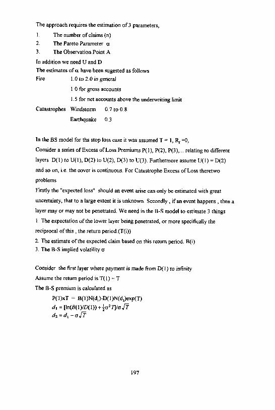
The approach requires the estimation of 3 parameters,

1. The number of claims (n)2. The Pareto Parameter a3. The Observation Point A

In addition we need U and DThe estimates of a have been sugested as followsFire 1.0 to 2.0 in general

10 for gross accounts

1.5 for net accounts above the underwriting limit

Catastrophes Windstorm 0.7 to 0.8

Earthquake 0.3

In the BS model for ths stop loss case it was assumed T = 1, Rf =0,

Consider a series of Excess of Loss Premiums P(l), P(2), P(3),. relating to different

layers D(1) to U(l), D(2) to U(2), D(3) to U(3). Furthermore assume U(l) = D(2)

and so on, i.e. the cover is continuous. For Catastrophe Excess of Loss theretwo

problems

Firstly the “expected loss” should an event arise can only be estimated with great

uncertainty, that to a large extent it is unknown. Secondly , if an event happens , then a

layer may or may not be penetrated. We need in the B-S model to estimate 3 things

1. The expectation of the lower layer being penetrated, or more specifically the

reciprocal of this , the return period.(T(i))

2. The estimate of the expected claim based on this return period. B(i)3. The B-S implied volatility

Consider the first layer where payment is made from D(1) to infinity

Assume the return period is T(l) = T

The B-S premium is calculated as

197

Consider an Excess of Loss with a return period of 4 years

Consider the following 4 layers

Layer 1 150 xs 100

Layer 2 750xs250

Layer 3 3000 xs l000

Layer 4 6000 xs 4000

The results of the calculation by the Pareto formula and BS is given below

Alpha B BS All Layer 2 Layer 3 Layer 4

Volatility Layer to Layer 4 to Layer 4

2 99 39 9 1.5

185 0.8 98 40 154 n/a

1.5 180 106 43 12

270 1 183 109 42 3,938

1 460 369 230 91

550 1.25 460 366 173 316

0.8 755 655 463 210

850 1.38 758 656 398 227

0.6 1,327 1,216 949 484

1,420 1.51 1,327 1,216 890 475

0.4 2,474 2,352 1,977 1,117

2,570 1,66 2,476 2,358 1,966 1,297

The calculations are made for different alphas. The first premium is that calculated by

assuming a Pareto distribution, and the second by the distribution free B-S approach.

This assumes n = 25, i.e. a return period of 4 years. Note the consistency in the low

alpha range for catastrophes.

198

Note

1 The B’s are intependent of the period of return and depend solely on alpha.

They are approximately equal to :Deductible plus Penetration x Expected Excess Claim

2. There is a consistent relationship between the BS volatility for all layers This

is given by

BS Volatility (Alpha 1) = BS Volatility (Alpha 2) X[ 1+[Alpha2 -Alpha1]

2]

Again this is independent of the return period.

What is perhaps surprising is the consistency in the results.

Pareto Calculations for T=4

PenetrationPenetration

Expected Excess ClaimExpected Excess Claim

PenetrationPenetration

Expected Excess ClaimExpected Excess Claim

PenetrationPenetration

Expected Excess ClaimExpected Excess Claim

PenetrationPenetration

Expected Excess ClaimExpected Excess Claim

PenetrationPenetration

Expected Excess ClaimExpected Excess Claim

PenetrationPenetration

Expected Excess ClaimExpected Excess Claim

Alpha

20

1.5

1.0

0.8

0.6

0.4

Layer 1 Layer 2 Layer 3 Layer 4

1.0000 0.1600 0.0100 0.0016

60 187.5 750 2,400

1.0000 0.2530 0.0316 0.0040

73 250 1,000 2,940

1.0000 0.4000 0.1000 0.0250

92 347 1,386 3,665

1.0000 0.4804 0.1585 0.0523

101 399 1,597 4,022

1.0000 0.5771 0.2512 0.1093

111 463 1,852 4,427

1.0000 0.6931 0.3981 0.2287

122 540 2,162 4,885

199

Curve Fitting

This method is fairly simple.

Rates from a number of contracts are represented as a rate on line versus the exposure

calculated on a consistent basis. An example might be as a percentage of the expected

loss should a storm like 90A repeat itself based on the current portfolio. The points

may be based on deductible. mid point of range, and upper limit.

Once these are graphed a curve of a sepcific type is plotted to get a good fit and

statistical limits are placed on the curve to identify outliers.

Examples of curves include negative exponentials with an upward shift (to represent a

minimum rate on line) athough other curves may also be used. There is a balance

between goodness of fit and the number of parameters

Table of Exposure versus Rate on Line

200

Appendix 1.6 Financial Models

Financial models have been used in practice to determine premium rates for a number

of classes in the United States. They have been used to determine the appropriate rate

required to give an equity holder in the company an appropriate “rate of return”. This

return is also supposed to take in the degree of risk. They do not appear to have been

used for reinsurance pricing, but there must be a strong possibility that the techniques

are explored for appropriate application in the future.

The key work is The Financial Theory of Pricing Property Liability Contracts by

D’Arcy and Doherty[]. They explore three models, the Capital Asset Pricing Model,

the Arbitrage Pricing Model and the Option Pricing Model. Note that the Option

Pricing model differs from that used in the relativistic pricing in section. Other financial

‘theory approaches include discounted cash flow, return on equity and other issues

dealt with elsewhere in this paper.

The Capital Assets Pricing Model.(CAPM)

This was applied in 1976 to automobile insurance rates in Massachusetts.

In Capital Asset Pricing Theory, the return required by an investor is expressed as a

linear function of the security BETAE(r) = rf + ß(E(rm) - rf)rf is the return on the securityrm is the market (or portfolio) returnß is the measure of market (or systematic) risk

The return on equity re on an insurance contract is given by

ru is the underwriting returnrt is the investment returnP are the written premiums

X are the costs (excluding capital costs) and x = X/P

k is the fond generating coefficient and is a corrective factor to allow for

the period over which funds earn interest.

Taking expectations we haveK(r) = [ 1 + k(P/JZ)( 1 - x)]E(r,) + (P/E)E(ru)

The investment returns are assumed to be in equilibrium, that is

201

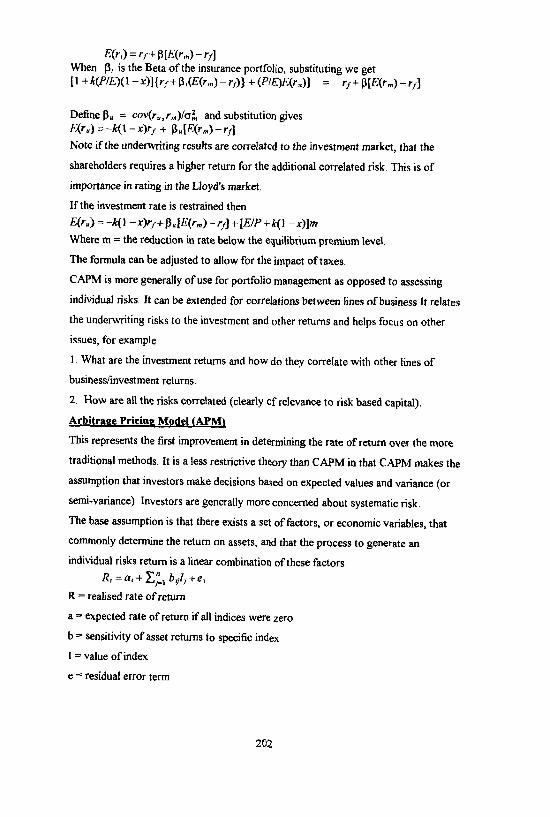
E(r1) = rf + ß[E(rm) - rf]When ß1 is the Beta of the insurance portfolio, substituting we get[1+k(P/E)(1-x)]{rf+ß1(E(rm)-rf)}+(P/E)E(Rn)]=rf+ß[E(rm)-rf]

Define and substitution givesE(ru) = -k(1-x)rf + ßu[E(rm)-rf]Note if the underwriting results are correlated to the investment market, that the

shareholders requires a higher return for the additional correlated risk. This is of

importance in rating in the Lloyd’s market

If the investment rate is restrained thenE(ru)=-k(1-x)rf+ßu[E(rm)-rf]+[E/P+k(1-x)]m

Where m = the reduction in rate below the equilibrium premium level

The formula can be adjusted to allow for the impact of taxes.

CAPM is more generally of use for portfolio management as opposed to assessing

individual risks. It can be extended for correlations between lines of business It relates

the underwriting risks to the investment and other returns and helps focus on other

issues, for example

1. What are the investment returns and how do they correlate with other lines of

business/investment returns.

2. How are all the risks correlated (clearly of relevance to risk based capital).

Arbitrage Pricing Model (APM)

This represents the first improvement in determining the rate of return over the more

traditional methods. It is a less restrictive theory than CAPM in that CAPM makes the

assumption that investors make decisions based on expected values and variance (or

semi-variance) Investors are generally more concerned about systematic risk.

The base assumption is that there exists a set of factors, or economic variables, that

commonly determine the return on assets, and that the process to generate an

individual risks return is a linear combination of these factors

R = realised rate of return

a = expected rate of return if all indices were zero

b = sensitivity of asset returns to specific index

I = value of index

e = residual error term

202

The pricing relationship is

E(r1) = where r1f = expected return on zero systematic risk

= excess return factor with only one unit of systematic risk of that factor and

no other systematic risk

These factors are determined by factor analysis as the bij from source data

For underwriting

These results look remarkably similar to many linear models used in alternative rating

strategies

Option Pricing Model

This is put forward as an extension of the above to be used primarily in rating

aggregate excess of loss contracts.

The formula is

PR = competitive price for reinsurance contract

rF = riskless interest rateRF=l+rf

t = corporate marginal tax rate = effective tax late on reinsurers investment income

k = funds generating coefficient

S = premium to surplus ratio for the reinsurer

D = deductible on the reinsurance contract

P = premium on direct contract (which is assumed to be competitive)

Nor(*) = cumulative standard normal density at *

nor(*) = standard normal density at *o(L) = standard deviation of loss distribution.

203

Where

θ

Data comes from four sources1. Not specific to the firm rf,12. Financial data specific to the reinsurer3. Data specific to the loss4. Data on direct insurance contract P

Using similar techniques as in Sanders[20], this approach could be extended to event

excess of loss contracts using return periods.

The formula assumes that the Central Limit Theorem applies. Non normal distributions

can be handled be these techniques, but some care is required

204

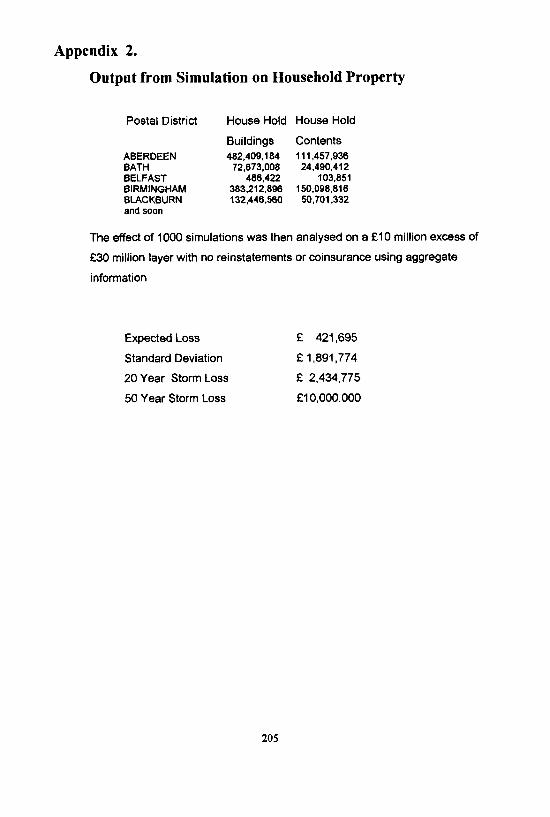
Appendix 2.

Output from Simulation on Household Property

Postal District

ABERDEEN BATH BELFAST BIRMINGHAM BLACKBURN and soon

House Hold House Hold

Buildings Contents

482,409,104 111,457,938 72,673,008 24,490,412

486,422 103,851 383,212,896 150,098,818 132,446,560 50,701,332

The effect of 1000 simulations was then analysed on a £l0 million excess of

£30 million layer with no reinstatements or coinsurance using aggregate

information

Expected Loss £ 421,695

Standard Deviation £ 1,891,774

20 Year Storm Loss £ 2,434,775

50 Year Storm Loss £ l0,000.000

205

Appendix 3

Tables From

“An Exposure Rating Approach to Pricing Property Excess

of Loss Reinsurance”

These tables give the Loss Distribution as a Percentage of Insured Value

The distributions are split into the following Policy Limit Ranges

1. $1,000 to $25,000

2. $25,000 to $100,000

3. $100,000 to $300,000

4. $300,000 to $1,000,000

5. In excess of $1,000,000

Losses are expresses as a percent if insured value at the levels of 5%, 10%, 20% and in

10% increments to 100%

The Distribution given are

Retail/Wholesale Risk, Fire Losses Only, Contents Only

Retail/Wholesale Risk. All Other Policies

All Commercial Combined Classes - Fire Losses Only

- Wind Losses Only

- ALL Other Losses

Retail/Wholesale Risks Only

Services/Office Risks

Restaurant Risks

- Fire Losses Only

- Wind Losses Only

- All Other Losses

- As above

- As above

206

Example All Commercial Property Classes - Wind Loss Only

Jnsurance Range

5 %

10%

20 %

30 %

40%

50 %

60%

70%

80 %

90%

100%

1,000 to 25,000 to 100,000 to 300,000 to Greater than

25,000 100,0a0 300,000 1,000,000 1 ,000,000

29.0 63.3 84.3 82.5 99.1

45.2 74.5 91.9 87.0 100.0

65.0 82.8 97.3 92.5 100.0

76.8 87.4 99.5 95.8 100.0

84.7 904 100.0 97.6 100.0

89.3 92.8 100.0 99.3 100.0

93.1 94.8 100.0 100.0 100.0

95.6 96.6 100.0 100.0 100.0

97.3 97.9 100.0 100.0 100.0

98.7 99.2 100.0 100.0 100.0

100.0 100.0 100.0 100.0 100.0

207

Bibliography

1.

2.

3

4

5

6

Beer R.A & Nemlick K.J PCAS 146 (1990) Pricing the Impact of Adjustable Features and Loss Sharing Provisions of Reinsurance

Treaties

Clark DR 1994 CAS Call Papers A Simple Tool for Pricing Loss Sensitive features of Reinsurance Treaties.

The Beer paper used just a lognormal distriibution to assess the cost, whereas Clark

uses a lognormal mixed with a Gamma. The advantage is that Clarks distribution is a

closed form and can be used more readily in spreadsheets. Cozzolino J.M. and Mikelaj PJ 1994 CAS Call Papers

Undewriting Best Share of Excess of Loss Stannard J N and John R T. PCAS 1990

Evaluation of the Effect of Reinsurance Contract Terms

This paper uses cash flow simulation techniques to measure the impact ofchanges in

contract terms.

7

8

9

Hogg R.A. and Klugman S.A

Loss Distributions Wiley 1984

Panjer HH and Wilmott GE

Insurance Risk Models Society of Actuaries 1992

Details the Distribution Calculus as well as describing the classical distributions.

Samorodnitsky G. and Taqqi M.S.

Stable Non Gaussian Random Processes Stochastic Models with Infinite Variance Chapman and Hail

Janicki A.and Weson A.

Simulation and Chaotic Behaviour of alpha stable stochastic processes Decker

Embrechts, Kuppelberg & Michovitch

Modelling of Extremal events in Insurance & Finance

Springer (To appear 1996)

208

10.

11.

12.

13.

14

IS

16

17

Kiln RJ

Reinsurance in Practice Witherby Kiln RJ

Reinsurance Underwriting DYP

Practical examples of how a top underwriter assesses both the risk and the premiums.

Excellent examples in the second volume.

Goovaerts, de Vylder and Haezendench

Insurance Premiums

Highly Mathematical and appears to be too general without any real practical

examples. Carriere J.F & Buhr K.A

Valuation of Carastrophe Insurance Contracts Using Compound Poisson Claim

Assumptions ARCH 1995.1

Falk M., Huusler J. & Rees R.A

Laws of Small Numbers: Extremes and Rare Events Birkhauser Verlag

A useful book with some real applications, Usefull for its associated XTREMES

programme which comes with the book

Casualty Actuarial Society The Foundations of Casualty Actuarial Science

Chapter 6 Reinsurance by Gary Patrick

Chapter 7 Credibility by Gary G Ventner Hertzog T.N.

Introduction to Credibility Theory ACTEX

This is the Casualty Actuarial text book which has replaced the famous Longley Cooke

paper” Ab introduction to Credibility Theory” OCAS 49 (1962). This book covers

most approaches and is an excellent introduction Brown RL Introduction to Ratemaking and Loss Reserving for Property and Casualty Insurance

Actex This is a basic book and is primarily concerned with direct insurance

209

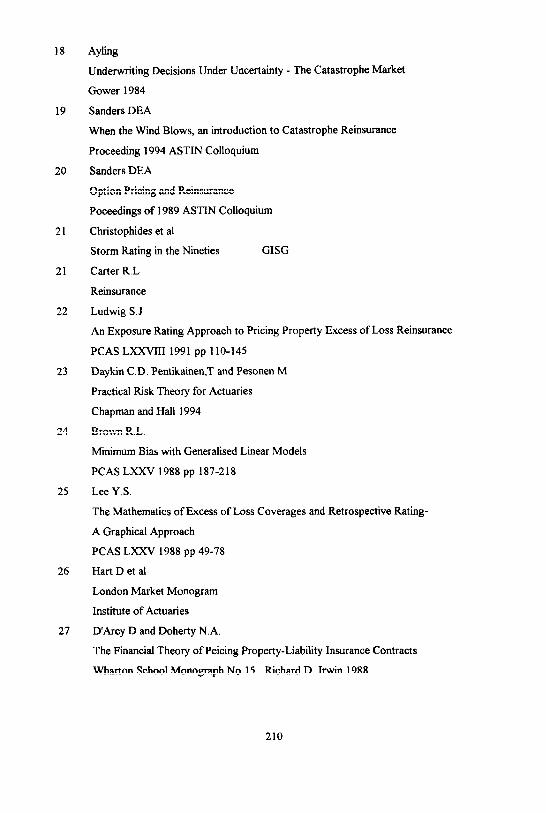
18

19

20

21

21

22

23

24

25

26

27 D’Arcy D and Doherty N.A. The Financial Theory of Peicing Property-Liability Insurance Contracts

Wharton School Monograph No 15 Richard D. Irwin 1988

Ayling Underwriting Decisions Under Uncertainty - The Catastrophe Market

Gower 1984

Sanders DEA When the Wind Blows, an introduction to Catastrophe Reinsurance

Proceeding 1994 ASTIN Colloquium

Sanders DEA Option Pricing and Reinsurance

Poceedings of 1989 ASTIN Colloquium

Christophides et al Storm Rating in the Nineties

Carter R.L

Reinsurance

Ludwig SJ

GISG

An Exposure Rating Approach to Pricing Property Excess of Loss Reinsurance

PCAS LXXVIII 1991 pp 110-145

Daykin C.D. Pentikainen,T and Pesonen M Practical Risk Theory for Actuaries

Chapman and Hall 1994

Brown R.L.

Minimum Bias with Generalised Linear Models

PCAS LXXV 1988 pp 187-218

Lee Y.S. The Mathematics of Excess of Loss Coverages and Retrospective Rating-

A Graphical Approach PCAS LXXV 1988 pp 49-78 Hart D et al London Market Monogram

Institute of Actuaries

210

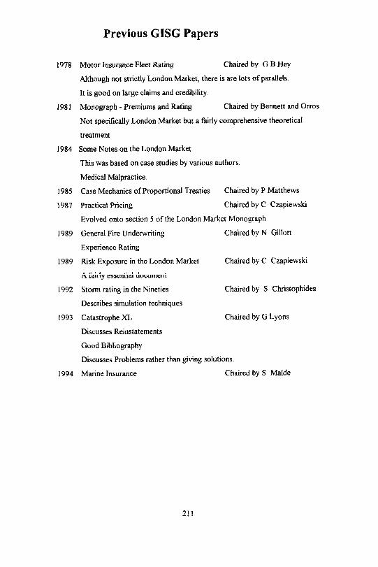
Previous GISG Papers

1978

1981

1984

1985

1987

1989

1989

1992

1993

1994

Motor Insurance Fleet Rating Chaired by G.B Hey

Although not strictly London Market, there is are lots of parallels.

It is good on large claims and credibility.

Monograph - Premiums and Rating Chaired by Bennett and Orros

Not specifically London Market but a fairly comprehensive theoretical

treatment

Some Notes on the London Market

This was based on case studies by various authors.

Medical Malpractice.

Case Mechanics of Proportional Treaties Chaired by P Matthews

Practical Pricing Chaired by C Czapiewski

Evolved onto section 5 of the London Market Monograph

General Fire Underwriting Chaired by N Gillott

Experience Rating

Risk Exposure in the London Market

A fairly essential document

Storm rating in the Nineties

Describes simulation techniques

Catastrophe XL

Discusses Reinstatements

Good Bibliography

Chaired by C Czapiewski

Chaired by S Christophides

Chaired by G Lyons

Discusses Problems rather than giving solutions.

Marine Insurance Chaired by S Malde

211