Pricing Information Goods:

A Strategic Analysis of the Selling and

Pay-per-use Mechanisms

_______________

Sridhar BALASUBRAMANIAN

Shantanu BHATTACHARYA

Viswanathan KRISHNAN

2011/118/TOM

Pricing Information Goods: A Strategic Analysis of the

Selling and Pay-per-use Mechanisms

Sridhar Balasubramanian*

Shantanu Bhattacharya**

Viswanathan Krishnan***

.

* Associate Professor of Marketingt at Kenan-Flagler Business School, University of North

Carolina, 300 Kenan Center Drive, Chapel Hill, NC 27599, USA.

Email: sridhar_balasubramanian@unc.edu

** Associate Professor of Operations Management at INSEAD, 1 Ayer Rajah Avenue, 138676

Singapore. Email: shantanu.bhattacharya@insead.edu

*** Professor and Sheryl and Harvey White Endowed Chair at Rady School of Management,

University of California San Diego, 9500 Gilman Drive 0553 La Jolla, California, USA.

Email: vkrishnan@ucsd.edu

A Working Paper is the author’s intellectual property. It is intended as a means to promote research to

interested readers. Its content should not be copied or hosted on any server without written permission

from publications.fb@insead.edu

Find more INSEAD papers at http://www.insead.edu/facultyresearch/research/search_papers.cfm

Pricing Information Goods: A Strategic Analysis ofthe Selling and Pay-per-use Mechanisms

Sridhar BalasubramanianUniversity of North Carolina at Chapel Hill, Sridhar Balasubramanian@unc.edu

Shantanu BhattacharyaINSEAD, shantanu.bhattacharya@insead.edu

Viswanathan KrishnanUniversity of California, San Diego, vkrishnan@ucsd.edu

We analyze two pricing mechanisms for information goods – selling, where an up-front payment allows

unrestricted use by the consumer, and pay per-use pricing where the payments are tailored to the consumer’s

usage patterns. We analytically model these pricing mechanisms in a market where consumers differ in

terms of usage frequency and utility-per-use. When a monopolist employs each mechanism independently, we

demonstrate that pay-per-use pricing generally yields higher profits than selling, provided the transaction cost

associated with the former is not too high. We then show that pay-per-use yields higher profits than selling

when usage frequency is uncertain, whereas selling yields higher profits when utility-per-use is uncertain. We

then analyze a duopoly and demonstrate that, in the only non-zero pricing equilibrium, one duopolist employs

selling and the other employs pay-per-use. Here, the findings from the monopoly case are reversed and selling

always yields higher profits than pay-per-use. Further, we demonstrate that as the transaction cost associated

with pay-per-use increases, the profits of both duopolists can increase. If an upgrade is to be offered later, we

show that if consumers are myopic, the pay-per-use mechanism performs better in a monopoly, and selling

performs better in a duopoly. Finally, we model the scenario where competing, vertically differentiated firms

can choose endogenously between the two pricing mechanisms and demonstrate how the firms move from

each offering both mechanisms when the transaction cost associated with pay-per-use is low to each offering

only selling when this cost is very high.

Key words : information goods, competitive strategy, pricing mechanisms

History :

1. Introduction

Advances in network technology have enhanced the popularity of “pay-per-use” pricing for infor-

mation goods (Altinkemer and Tomak 2001, Choudhary et al. 1998). With the rapid growth of

Cloud-based computing and information management,the pay-per-use model is now increasingly

being applied across usage settings including gaming and movies (Altinkemer and Bandyopadhyay

2000, Krause 2004, Machrone 2006), data plans (Chavez 2011), information storage (Clark 2011),

monetary transactions (Reeve 2011), teleconferencing (McKnight and Boroumand 2000), billing

1

2

services, software applications such as Salesforce.com that now allow payment on a “per-login”

basis, and Computer Aided Design (CAD) suites (Machine Design 2000). In this paper, we analyze

the performance of conventional selling (i.e., unlimited-use pricing) and pay-per-use mechanisms

for information-intensive goods in monopoly and duopoly contexts.

Pricing has been described as the moment of truth in the marketing context (Corey 1991), and

is sensitive to consumer usage patterns and heterogeneity (Chen et al. 2001). Independent of how

much value the company has created for customers, a bad pricing decision can lower profits either

because the company tries to extract too much value back from the customer, or because the

company leaves too much value on the table for the customer. In particular, when it comes to

information goods, pay-per-use and other technology-intensive pricing strategies can play a key

role in enhancing the value delivered to the customer, in facilitating better extraction of created

value, and ultimately, in altering the competitive landscape (Nault and Dexter 1995).

To motivate the theoretical development, consider the application of pay-per-use pricing in the

engineering design industry. Altair Engineering’s Hyperworks On-Demand is a computer-aided

engineering (CAE) simulation software platform that is applied by clients to create virtual models

that can aid structural optimization (Roush 2011), and the study of fluid-structure interaction

and multi-body dynamics (e.g., collisions between “virtual” cars). Under a “pay-per-usage” license

model, customers purchase HyperWorks “units” which are used to pay for the metered use of a

suite of HyperWorks products that are hosted in the Cloud. Altair highlights four key benefits of

the pay-per-use pricing model: (a) Flexibility – the client can avoid scaling up or scaling down

any hardware capacity in response to demand peaks and valleys; (b) Efficiency – the hardware

capabilities and solutions employed by Altair will handle workloads better that a typical client’s

in-house infrastructure; (c) Accessibility – the client can access the platform from any physical

location; and (d) Security – each client’s data is safely partitioned and stored in the Cloud.

In contrast to renting or leasing, which typically confer complete usage rights on the consumer

for a limited temporal period, pay-per-use tightly links the consumer’s usage patterns to payment

(Altman and Chu 2001). This makes pay-per-use more appealing than selling to consumers with

low usage frequencies (Nicolle 2002). Despite this benefit, there is an ongoing debate about the

relative advantages of pay-per-use pricing compared to selling (Bonasia 2007). We demonstrate

how the strength of each mechanism varies as a function of consumers’ utility-per-use and usage

frequency, and across monopoly and duopoly contexts. Our analysis contributes to the literature

and practice by addressing the following questions, among others: How do conventional selling and

pay-per-use pricing perform in markets where consumers differ in terms of (a) utility-per-use and

3

(b) usage frequency? How do sellers and pay-per-use providers compete for such a market? How

do competing firms that offer vertically differentiated information goods endogenously choose a

pricing strategy?

Our analysis delivers several findings across monopoly and duopoly contexts. Some key findings

are briefly summarized as follows. First, consider a monopolist who chooses between selling and

pay-per-use pricing. Here, pay-per-use yields higher profits provided the transaction cost associated

with it is not too high. Further, consumer surplus is generally higher under selling; in contrast,

social surplus is higher under selling only when the transaction cost associated with pay-per-use

is low. We also study the impact of demand uncertainty in either the frequency of usage or the

utility-per-use on both mechanisms, and find that uncertainty in usage frequency favors the pay-

per-use mechanism, whereas uncertainty in utility-per-use favors the selling mechanism. If the firm

can offer upgrades later, we find that in a monopoly, the pay-per-use mechanism performs better

than the selling mechanism.

Second, we consider the case where duopolists that offer identical products can choose any one,

or both, of the pricing mechanisms. Here, we demonstrate that, in equilibrium, one firm sells the

good, and the other employs pay-per-use. Further, in contrast to the monopoly, selling strongly

outperforms pay-per-use pricing in a duopoly. An interesting finding here is that the profits of the

pay-per-use provider are inverted-U shaped with respect to the transaction costs associated with

that mechanism. We demonstrate that a higher transaction cost can reduce competitive pressure

and allow the profits of both firms to increase. If the firm can offer upgrades later, we find that in

a duopoly, selling performs better than the pay-per-use mechanism.

Following that, we consider the case where duopolists with vertically differentiated information

goods can employ either one or both mechanisms. Here, we show that the pay-per-use mechanism

makes a minor contribution to the profits of each firm but plays an important role in enhancing

the profits from selling. We also demonstrate how the equilibrium choices of pricing mechanisms

by the firms vary as a function of the transaction cost associated with the pay-per-use mechanism.

We also consider how the relative attractiveness of the pricing mechanisms is affected by other

factors, including: (a) uncertainty about consumer utility-per-use and/or usage frequency; (b) the

possibility of upgrades being offered by the firm; (c) alternative (non-uniform) distributions of these

utility dimensions; and (d) implementation and service costs encountered in enterprise contexts.

1.1. Extant Literature and Contribution

Research on renting versus selling in economics and marketing has primarily focused on the durable

goods context. The key theme here is the seller must coordinate primary and secondary markets

4

to maximize profits (Bulow 1982, Desai and Purohit 1998, Shulman and Coughlan 2007). An

advantage of selling is that it can help “lock up” the market when there is a threat of competitive

entry (Bucovetsky and Chilton 1986). Similarly, in a competitive environment in the auto industry,

Desai and Purohit (1999) find that competitors do not lease all their units, but they either use a

combination of both leasing and selling, or only selling. They also find that the fraction of leasing

decreases as the manufacturer’s products become more similar, and the competition between them

increases. Finally, Purohit (1997) and Bhaskaran and Gilbert (2009) compare leasing and selling

when manufacturers have multiple competing intermediaries. We make a number of contributions to

this stream of literature. First, whereas the existing literature has considered competition between

a designated seller and a designated pay-per-use provider (Fishburn and Odlyzko 1999), we analyze

the equilibrium that involves the endogenous choice of the selling and/or pay-per-use by a pair of

competing firms. In this context, we derive a “defensive positioning” outcome – specifically, the

firm may choose pay-per-use in a monopoly, but if it expects competition, it can protect profits

by selling the good. Additionally, we demonstrate that as the transaction cost associated with

pay-per-use increases, the profits of both duopolists can increase. Second, we move beyond the

existing literature by analyzing the more general equilibrium where duopolists who offer vertically

differentiated goods can choose either or both of the pricing mechanisms. Here, we demonstrate how

the market is divided among the competing mechanisms, and show that when the transaction cost

associated with pay-per-use is: (a) at low to moderate levels, both firms employ both mechanisms;

(b) high, then the firm that offers higher quality employs both mechanisms, but the competitor

only engages in selling; and (c) very high, then both firms only sell the good.

Second, in the context of durable goods, the impact of demand uncertainty on the leasing and

selling mechanisms has been studied by Desai et al. (2007), who find that demand uncertainty

causes the producer’s inventory level to be U-shaped in the durability of the product, and leasing

causes a larger loss due to uncertainty than selling the product. We contribute to this stream of

literature by showing that demand uncertainty has different effects if the uncertainty is in the usage

frequency (in which case, the pay-per-use mechanism performs better), or in the utility-per-use (in

which case, selling performs better). The impact of upgrades has been studied by Yin et al. (2010)

in the durable goods sector, and Sankaranarayan (2007) for information goods. Yin et al. (2010)

find that frequent product upgrades are caused by the existence of electronic peer-to-peer markets,

and the interaction of these markets with the markets for retail goods. Sankaranarayan (2007)

finds that frequent new version releases of software result in lowering the developer’s profits due to

the strategic delaying of purchasing the software by consumers, and an offer by the developer of a

5

warranty for new versions solves this commitment problem. Providing software as a service can also

lead to lower investments in quality in the long run compared to the case where the software is sold

under a perpetual license (Choudhary 2007). We contribute to this stream of literature by showing

that for information goods, the introduction of upgrades favors the pay-per-use mechanism in a

monopoly, and selling in a competitive environment.

A number of studies in the durable goods context has examined the choice of leasing or sell-

ing for a monopolist. Desai and Purohit (1998) find that the relative profitability of leasing and

selling hinges on the rates at which leased and sold units depreciate, and if sold units depreciate

significantly faster than leased units, then selling is the better option. If both units depreciate

at different rates, then the firm should use a combination of leasing and selling. Bhaskaran and

Gilbert (2005) find that in durable goods, a manufacturer that leases its products charges a higher

price by limiting the availability of the product in response to the availability of a complement.

Finally, Chien and Chu (2008) show that profits from selling durable goods is higher than from

leasing durable goods, as selling durable goods creates a stronger customer base using penetration

pricing.

In the study of information goods as well, selling and renting may not be mutually exclusionary –

a monopolist can optimally employ both mechanisms when consumer preferences are heterogeneous

and future upgrades are of uncertain quality (Zhang and Seidmann 2003). Similarly, Zhang and

Seidmann (2010) demonstrate that, in the presence of quality uncertainty and network effects,

the firm should offer both the selling and pay-per-use mechanisms as this increases both profits

and consumer welfare. Other studies of electronic goods pricing include pricing of online services

(Essegaier et al. 2002, Gurnani and Karlapalem 2001, Jain and Kannan 2002), and the interaction

of pricing of online goods and product customization (Dewan et al. 2003). Postmus et al. (2009)

compare selling and the pay-per-use mechanism with software development costs, and find that

pay-per-use dominates if software development is expensive, while selling dominates if development

costs are low. Sundararajan (2004) compares the selling and pay-per-use (usage based) mechanisms

in a monopoly setting and derives conditions where a combination of usage based pricing and selling

should be used. In contrast, our analyses throughout correspond to the case where consumers are

jointly differentiated in terms of both usage utility and usage frequency for information goods. Jiang

et al. (2007a) consider a similar differentiation and show that selling is optimal when consumers

have homogeneous valuations, but pay-per-use is more profitable than selling in markets with

heterogeneous consumers and low user inconvenience costs, when there is the potential of piracy

in the market. The presence of network effect also favors pay-per-use over selling. We show that if

6

a monopolist wants to choose one mechanism, it should prefer pay-per-use if transaction costs are

low, and selling if transaction costs are high. If both mechanisms can be used, then pay-per-use

is used to cover a larger share of the market if transaction costs are low, and a lower share of the

market if transaction costs are high.

Overall, our research contributes to the literature in a number of ways. Our analyses throughout

correspond to the case where consumers are jointly differentiated in terms of both usage utility

and usage frequency. This approach reveals some interesting insights that are unavailable in the

literature. In a monopolistic environment, the pay-per-use mechanism performs better in a wider

variety of cases if transaction costs are low, while selling dominates in a competitive environment

even when transaction costs are low. When transaction costs are high, selling performs better than

the pay-per-use mechanism. On balance, much remains to be studied about how usage-sensitive

pricing mechanisms can create a strategic advantage (Ba and Johansson 2006). Our work takes a

step towards filling in some of the knowledge gaps.

The base model is introduced in Section 2. In Section 3, the pricing mechanisms are analyzed

in both monopoly and duopoly contexts. In Section 4, we analyze competition with differentiated

goods. Model extensions and tests for robustness are presented in Section 5. We conclude with

Section 6.

2. The model2.1. Assumptions and notation

Assumption 1 : Consumers purchase the information good, pay for it per use, or abstain from the

market after considering the benefits over a N -period horizon.

Assumption 2 : Each consumer i is characterized by the coordinate pair (θi,φi), where θi is the

expected usage frequency of consumer i in any period and φi is the associated utility-per-use.

Assumption 3 : Usage utility φ is distributed U [0, φH ] and usage frequency θ is distributed

U [0, θH ]. The upper limits of the distributions are elastic – this captures a range of market struc-

tures and consumer behaviors. For example, if θH > 1, consumers can use the good multiple times

per period. The situation where θ is distributed U [0,1] is a special case where θi represents the

probability of use in a given period.

Assumption 4 : Consumers using pay-per-use incur a transaction cost T per usage occasion. This

cost reflects the disutility from the repeated administrative and transaction costs associated with

pay-per-use pricing (Varian 2000, Cheng et al. 2003). For example, to play a game from an online

site, the consumer may need to first establish some authentication. The transaction cost could

7

also capture the “ticking meter” effect that results when payment is tightly linked to consumption

(Train 1991). When usage experiences in the pay-per-use and selling mechanisms converge, T=0.

Assumption 5 : Reflecting a perfect capital market, the discount factor for future utility, δ, is the

same for the firm and consumers.

Assumption 6 : The information good can be reproduced and delivered at negligible marginal cost.

Further, we ignore fixed costs because they do not directly impinge on optimal pricing decisions.

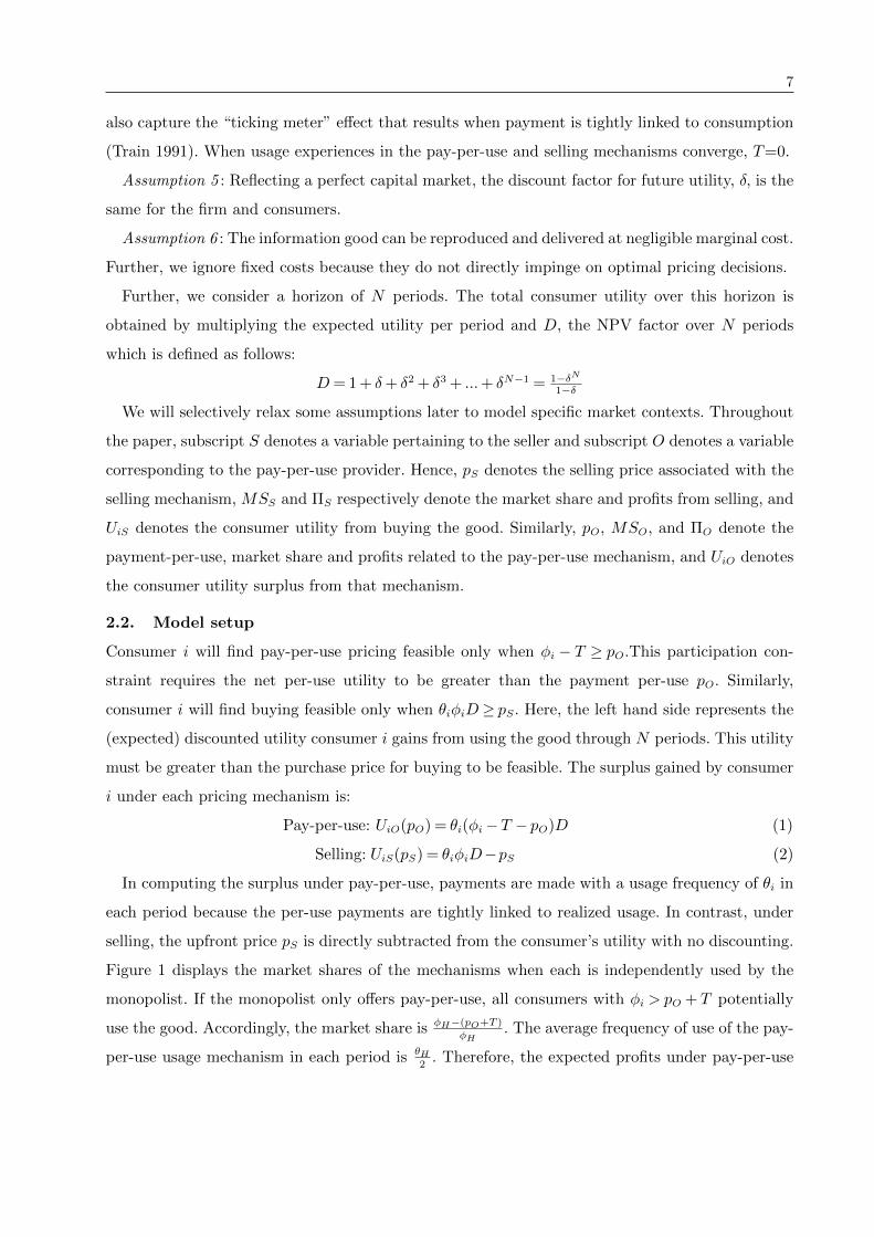
Further, we consider a horizon of N periods. The total consumer utility over this horizon is

obtained by multiplying the expected utility per period and D, the NPV factor over N periods

which is defined as follows:

D= 1 + δ+ δ2 + δ3 + ...+ δN−1 = 1−δN1−δ

We will selectively relax some assumptions later to model specific market contexts. Throughout

the paper, subscript S denotes a variable pertaining to the seller and subscript O denotes a variable

corresponding to the pay-per-use provider. Hence, pS denotes the selling price associated with the

selling mechanism, MSS and ΠS respectively denote the market share and profits from selling, and

UiS denotes the consumer utility from buying the good. Similarly, pO, MSO, and ΠO denote the

payment-per-use, market share and profits related to the pay-per-use mechanism, and UiO denotes

the consumer utility surplus from that mechanism.

2.2. Model setup

Consumer i will find pay-per-use pricing feasible only when φi − T ≥ pO.This participation con-

straint requires the net per-use utility to be greater than the payment per-use pO. Similarly,

consumer i will find buying feasible only when θiφiD≥ pS. Here, the left hand side represents the

(expected) discounted utility consumer i gains from using the good through N periods. This utility

must be greater than the purchase price for buying to be feasible. The surplus gained by consumer

i under each pricing mechanism is:

Pay-per-use: UiO(pO) = θi(φi−T − pO)D (1)

Selling: UiS(pS) = θiφiD−pS (2)

In computing the surplus under pay-per-use, payments are made with a usage frequency of θi in

each period because the per-use payments are tightly linked to realized usage. In contrast, under

selling, the upfront price pS is directly subtracted from the consumer’s utility with no discounting.

Figure 1 displays the market shares of the mechanisms when each is independently used by the

monopolist. If the monopolist only offers pay-per-use, all consumers with φi > pO + T potentially

use the good. Accordingly, the market share is φH−(pO+T )

φH. The average frequency of use of the pay-

per-use usage mechanism in each period is θH2

. Therefore, the expected profits under pay-per-use

8

Figure 1 Market shares for pay-per-use pricing and selling

φΗ

θH

0

Pay-per-use

fraction

Uncovered

market

pO

pO+T

φΗ

θH

0

Uncovered

market

pS=θφD

Buying

fraction

are:

ΠO(pO) = φH−(pO+T )

φH

θH2pOD (3)

If the firm sells the good, all consumers with usage frequencies in the range θ ∈ [ pSφD, θH ] derive

(weakly) positive utility from buying the good. The market share of the seller and the resulting

profits are, respectively:

MSS(pS) = 1φHθH

∫ φHφ=

pSθHD

[θH − pSφD

]dφ= 1φHθH

[θHφH − pSD

+ pSD

log( pSθHφHD

)]

ΠS(pS) =MSS(pS)pS = pSφHθH

[θHφH − pSD

+ pSD

log( pSθHφHD

)] (4)

The model provides a parsimonious and flexible representation of selling and pay-per-use mech-

anisms.

3. Pricing in monopoly and duopoly contexts3.1. Monopoly

We first analyze the separate use of each mechanism by a monopolist. The results are tabulated in

Table 1 (see Appendix A1 for proof).Pay-per-use Selling

Payment per use/Selling price pO = φH−T2

pS = 0.285θHφHD

Market share MSO = φH−T2φH

MSS = 0.358

Profits 18

θH (φH−T )2

φHD 0.1018θHφHD

Consumer Surplus 116

θH (φH−T )2

φHD 0.0769θHφHD

Social Welfare 316

θH (φH−T )2

φHD 0.1787θHφHD

Table 1: Optimal outcomes in a monopoly

Proposition 1: If the monopolist uses only pay-per-use pricing or selling, the profits from pay-

per-use pricing are higher than those from selling if T < 0.0976φH . The net consumer surplus is

9

always higher under selling, but the total social welfare under pay-per-use is higher than that under

selling if T < 0.0237φH .

A monopolist prefers pay-per-use when T is low, consistent with Sundararajan (2004). Intuitively,

pay-per-use perfectly discriminates among consumers in terms of usage frequency. This is because,

if the total cost per use – the sum of pO and T – is lower than the utility-per-use, consumers will

use the product on every occasion that they need to. This total cost is low when T is low, thereby

increasing market share and profits. In contrast, under selling, forward-looking consumers make

purchase decisions by comparing their total utility across time – this depends on both utility-per-

use and usage frequency – to the selling price. Therefore, selling is relatively more attractive than

pay-per-use for consumers with a low per-use utility but a high usage frequency (see Figure 1). The

level of T decides which of these contrasting benefits translate into higher profits. Another insight

is that, because the per-use payment is set to maximize profits on a period-by-period basis, the

optimal per-use payment and corresponding market share are independent of the usage frequency

and the NPV factor D (see Table 1).

Consumers have a higher net surplus under selling because, unlike pay-per-use, the firm that

sells cannot discriminate perfectly along the usage frequency dimension. Interestingly, even when

T = 0,the net consumer surplus under pay-per-use is lower than that under selling. However, the

increased profitability from pay-per-use ensures that for very low transaction costs (T < 0.0237φH),

the social welfare under pay-per-use is higher than under selling.

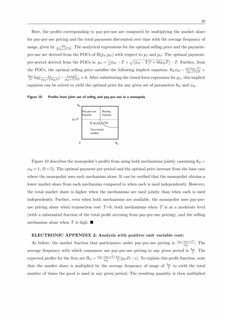
We extend these findings in two directions. First, consider the case where the monopolist jointly

offers both mechanisms. Here, only consumers with usage frequency higher than a certain critical

frequency given by θc = pS(pO+T )D

will buy the good, and others will prefer pay-per-use. We demon-

strate that the monopolist employs only pay-per-use when T = 0, and only selling as T approaches

φH . For intermediate levels of T , the monopolist employs both mechanisms. The role of pay-per-use

in generating profits decreases as T increases (see Electronic Appendix 1 for proof).

Second, consider the case where the good has positive marginal costs, possibly due to some

material content. We demonstrate that such costs decrease profits more sharply from pay-per-use

than from selling. Intuitively, under selling, there is a dedicated unit variable cost allocated to

each consumer who buys the good. In contrast, the allocation of supply to demand is more finely

controlled under pay-per-use. For example, as noted by Varian (2000), the same DVD at a rental

outlet can be shared by different consumers at different points of time – therefore, variable costs can

be allocated across a wider consumer base. Such “resource pooling” enhances profits (see Electronic

Appendix 2 for proof).

10

Moving forward from the “base case,” we now examine how uncertainty in usage frequency and

utility-per-use affect the performance of these mechanisms.

3.2. Uncertainty in usage frequency and utility-per-use

In this section, we consider the impact of uncertainty in the usage frequency and utility-per-use

separately first, and then jointly. In the case where only the usage frequency is uncertain, let the

usage frequency be distributed U [0, θH + v] with probability 0.5, and U [0, θH − v] with probability

0.5 (as before, utility-per-use is distributed U [0, φH ]). Similarly, in the case where only the utility-

per-use is uncertain, let the utility-per-use be distributed U [0, φH + v] with probability 0.5, and

U [0, φH − v] with probability 0.5 (the usage frequency is distributed U [0, θH ]). We can show that

any other binary probability combinations will not affect our findings. Here, v captures the degree of

uncertainty, and v= 0 implies the absence of uncertainty. We find that (see Electronic Appendices

3A and 3B for proof):

Proposition 2: (i) If the usage frequency is uncertain, the cut-off transaction cost below which

pay-per-use is more profitable than selling is higher than in absence of uncertainty.

(ii) If the utility-per-use is uncertain, the cut-off transaction cost below which pay-per-use is more

profitable than selling is lower than in the absence of uncertainty.

Effectively, uncertainty in usage frequency increases the relative attractiveness of the pay-per-use

mechanism. Recall that, under pay-per-use, a consumer pays for the good contingent on usage.

If consumers use the information good more or less frequently compared to the expected usage

frequency, the (risk neutral) firm still performs as well on average with the payment-per-use set

at the same level as in the case with no uncertainty. That is, there is no efficiency loss from such

uncertainty. In contrast, under selling, if the firm persists with same selling price as in the case

without uncertainty, then it loses market share if the actual distribution of usage frequency is at

the high end, and loses margin if that distribution is at the low end. Hence, the firm prices lower

under such uncertainty, reducing its profits.

In contrast, the expected profits under both mechanisms decrease when utility-per-use is uncer-

tain, but profits under pay-per-use decrease more sharply. Therefore, such uncertainty increases

the attractiveness of selling. The intuition is as follows. When the firm employs pay-per-use, its

market share is driven solely by utility-per-use because pay-per-use discriminates perfectly across

consumers in terms of usage frequency. Uncertainty regarding utility-per-use lowers the market

share under pay-per-use sharply because the firm is forced to choose a substantially lower payment-

per-use that can reasonably accommodate both the possible scenarios. On the other hand, selling is

less affected because the usage frequency, which plays a role in the construction of consumer utility

11

when evaluating the pricing mechanism, is known to the firm. Therefore, uncertainty along the

usage frequency and utility-per-use dimensions have distinct implications for each pricing mecha-

nism.

Next, consider the case where there is uncertainty in both usage frequency and utility-per-use.

We find that dual uncertainty lowers profits under pay-per-use to a lesser extent than under selling

(see Electronic Appendix 3C for a numerical analysis). This is because pay-per-use is negatively

affected only by uncertainty in utility-per-use whereas selling is negatively affected by both sources

of uncertainty.

3.3. Duopoly with undifferentiated information goods

Consider a duopoly where each firm can employ either selling or pay-per-use, or both mechanisms.

We model this game in two stages, where each firm chooses their mechanisms in the first stage, and

then given their choice of mechanisms, they choose their prices in the second stage (Coughlan 1985,

Gupta and Loulou 1998). Each firm’s good offers utility-per-use φ to consumers, and consumers

have the same usage frequency θ for both products. Result 1 summarizes the equilibrium outcome

for the channel choice game (see Electronic Appendix 4 for proof):

Result 1: Consider a duopoly with undifferentiated information goods. In the corresponding

Nash equilibrium, one firm employs selling and the other employs pay-per-use. There exists no

Nash equilibrium with positive firm profits where either firm employs both mechanisms, or both

firms employ the same mechanism.

If both firms employ the same mechanism, they compete themselves down to zero profits. Each

firm can lower its selling price or the payment-per-use to undercut the other – this cycle of under-

cutting will lead to a zero-profit outcome.

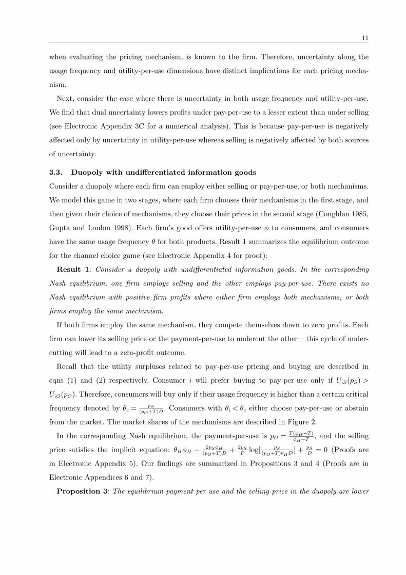
Recall that the utility surpluses related to pay-per-use pricing and buying are described in

eqns (1) and (2) respectively. Consumer i will prefer buying to pay-per-use only if UiS(pS) >

UiO(pO). Therefore, consumers will buy only if their usage frequency is higher than a certain critical

frequency denoted by θc = pS(pO+T )D

. Consumers with θi < θc either choose pay-per-use or abstain

from the market. The market shares of the mechanisms are described in Figure 2.

In the corresponding Nash equilibrium, the payment-per-use is pO = T (φH−T )

φH+T, and the selling

price satisfies the implicit equation: θHφH − 2pSφH(pO+T )D

+ 2pSD

log[ pS(pO+T )θHD

] + pSD

= 0 (Proofs are

in Electronic Appendix 5). Our findings are summarized in Propositions 3 and 4 (Proofs are in

Electronic Appendices 6 and 7).

Proposition 3: The equilibrium payment per-use and the selling price in the duopoly are lower

12

Figure 2 Market shares for pay-per-use pricing and selling in duopoly

φΗ

θH

0

Pay-per-use

fraction

Uncovered

market

pO+T

Buying

fraction

θc=pS/(pO+T)D

than the corresponding optimal payment-per-use and selling price when a monopolist uses the mech-

anisms independently. However, the equilibrium payment-per-use of the pay-per-use provider in the

duopoly first increases, and then decreases with transaction cost (T).

Figure 3 Selling price and payment-per-use in base case and duopoly

Seller's price w ith T

0

0.2

0.4

0.6

0.8

1

1.2

1.4

1.6

0 0.1 0.3 0.4 0.6 0.7 0.9

Transaction cost T

Se

lle

r's

pri

ce

Duopoly

Base

On-demand per-period payment with T

0

0.1

0.2

0.3

0.4

0.5

0.6

0 0.1 0.3 0.4 0.6 0.7 0.9

Transaction cost T

Pe

r-p

eri

od

pa

ym

en

t

Duopoly

Base

Proposition 3 captures the price suppressing effect of competition. However, in addition, there

are some subtle and interesting forces at work here (see Figures 3, 4 and 5 for a comparison of

prices, profits, and market shares across the base case and the duopoly (plotted for θH = φH = 1,

D = 5). In the duopoly, one would expect that payment-per-use and profits of the pay-per-use

provider are high when the associated transaction cost (T ) is low. However, when T is very low,

both the payment-per-use and the profits of pay-per-use provider are low. Both initially increase as

T increases, leading to the increasing part of the inverted U-shaped profit function. The intuition

is that, when T is very low, the seller has to sharply lower prices to attract consumers – this

enhances competition and lowers profits across the board. As T increases, the competitive pressure

13

decreases and the profits of both firms increase. However, as T increases even further, the profits

of the pay-per-use provider begin to decrease because that mechanism is ultimately less attractive

from the consumer’s viewpoint.

Figure 4 Profits from selling and pay-per-use pricing in base case and duopoly

0

0.1

0.2

0.3

0.4

0.5

0.6

0 0.1 0.3 0.4 0.6 0.7 0.9

Transaction cost T

Se

lle

r's

pro

fits

Duopoly

Base

0

0.1

0.2

0.3

0.4

0.5

0.6

0.7

0 0.1 0.3 0.4 0.6 0.7 0.9

Transaction cost T

Pa

y-p

er-

us

e p

rofi

ts

Duopoly

Base

Proposition 4: In a duopoly, the profits of the seller are always higher than those of the firm

that offers pay-per-use pricing.

Proposition 4 is interesting in several respects. Recall that when T is low, a monopolist will prefer

pay-per-use pricing over selling. However, in a duopoly, the seller’s profits are higher even when T

is low. The intuition is as follows. When the pay-per-use provider increases its payment-per-use,

it loses substantial revenues because all consumers with a utility per-use that is lower than that

payment drop out, taking the entire temporal stream of revenue associated with them. In contrast,

under selling, the usage frequency contributes to the total projected utility of the consumer and

ties the consumer to the selling mechanism. Further, selling captures the “best” consumers – those

with high utility-per-use and high usage frequency in a duopoly – leaving the less attractive fraction

of the market to the pay-per-use mechanism (see Figure 2). The ability of pay-per-use to allow

consumers to flexibly tailor payments to usage is a strength in the monopoly context. The reverse

side of the coin, though, is the inability of pay-per-use pricing to lock in consumers at an early

stage. This inability has no adverse consequences in a monopoly, but hurts the mechanism in a

duopoly.

Propositions 1 and 4 jointly offer some interesting insights on the choice of both mechanisms.

When T is low, a firm will adopt pay-per-use if it does not expect competition. However, if it expects

14

competition, it will sell the good instead. That is, the firm will adopt a “defensive positioning”

strategy, where it accepts lower profits which are more robust in the face of competition, rather

than higher profits that are susceptible to significant erosion on competitive entry.

The consumer surplus and social welfare generated by the selling and the pay-per-use mechanisms

are derived in Electronic Appendix 8 and plotted in Figure 13 in the Electronic Appendix. When T

is low, the consumer surplus and social welfare generated by the pay-per-use mechanism is higher

because the firm is forced to offer a low payment-per-use. When T is high, the consumer surplus

and social welfare generated by selling are higher.

Figure 5 Selling and pay-per-use market shares in base case and duopoly

0

0.1

0.2

0.3

0.4

0.5

0.6

0 0.1 0.3 0.4 0.6 0.7 0.9

Transaction cost T

Se

lle

r's

ma

rke

t s

ha

re

Duopoly

Base

0

0.1

0.2

0.3

0.4

0.5

0.6

0 0.1 0.3 0.4 0.6 0.7 0.9

Transaction cost T

Pa

y-p

er-

us

e m

ark

et

sh

are

Duopoly

Base

3.4. Selling and pay-per-use pricing with upgrades

In this section, we consider the impact of a future upgrade to the information good in a monopoly

(where the monopolist can choose either selling or pay-per-use pricing) and in a duopoly (where

one firm chooses selling and the other chooses pay-per-use pricing), where the upgrade is a part of

the sequential product introduction strategy of the firm (Padmanabhan et al. 1997). We assume

that consumers are myopic, myopic consumers have no foresight regarding the introduction of the

upgrade. Therefore, the upgrade will introduce no competitive effect because these consumers will

initially choose between selling and pay-per-use pricing solely based on the base information good.

Later on, these consumers will simply decide whether or not to purchase the upgrade.

Let the upgrade be introduced in period k, where k <N . The consumer obtains a higher per-use

utility of aφ (a > 1) from the upgrade. Therefore, post-upgrade, the per-use utility is uniformly

15

distributed between 0 and aφH . Let Dk−1 denote the NPV factor over k−1 periods (Dk−1 = 1−δk−1

1−δ ),

and D denote the NPV factor over N periods (as before).

3.4.1. Upgrades in a monopoly First, consider a monopolist who adopts pay-per-use pricing

in a market where consumers are myopic. The profits from the base good and the upgrade are

denoted by, respectively:

ΠO1(pO1) = φH−(pO1+T )

φH

θH2pO1Dk−1 ; ΠO2(pO2) = aφH−(pO2+T )

aφH

θH2pO2(D−Dk−1) (5.1)

The total profits are ΠO = ΠO1 + ΠO2 (from eqn 5.1). Because the upgrade delivers a higher

utility, the firm charges a higher per-use payment after the upgrade has been introduced (the

optimal per-period payments are derived in the Electronic Appendix 9).

Second, consider the case where the monopolist employs selling in a market where consumers

are myopic. Here, the base good will be priced exactly as in the monopoly without upgrades and

profits are identical to that case as well (see eqn. (4) for the profit expression). Consumers only

pay for the additional utility derived from the upgrade. If the upgrade is introduced in period k,

this additional surplus is: (a− 1)φθ(D−Dk−1)− δk−1pU . This additional surplus is set to zero to

find the fraction of consumers who will buy the upgrade. This condition is structurally identical

to that which applies when consumers decide whether or not to buy the base good. Therefore, all

consumers who purchase the base good will also choose to upgrade. The profits from the upgrade

alone (ΠS2) are denoted by:

ΠS2(pU) = δk−1pUMSS2 = δk−1pUφHθH

[θHφH− δk−1pU(a−1)(D−Dk−1)

+ δk−1pU(a−1)(D−Dk−1)

log( δk−1pU(a−1)θHφH (D−Dk−1)

)](5.2)

When consumers are myopic, the monopolist first solves for the optimal price of the base good.

Given the optimal price pS1 for the base good, the firm then solves for the optimal upgrade price

that maximizes the profits denoted in eqn. (5.2) above. In doing so, the monopolist must ensure

that MSS2 ≤MSS1,so that only a subset of consumers who purchased the base good will purchase

the upgrade. This condition is satisfied because all consumers who purchased the base good will also

buy the upgrade. With this setting, the key finding here is summarized as follows (See Electronic

Appendix 9 for proof):

Proposition 5: If a monopolist offers the information good with a future upgrade, then the

cut-off transaction cost below which pay-per-use pricing yields higher profits than selling is higher

compared to the case where the firm only offers the basic information good. Therefore, the presence

of the future upgrade increases the relative attractiveness of pay-per-use pricing compared to selling.

In a monopoly, the cut-off transaction cost below which pay-per-use pricing is superior to selling

is TC = 0.0976φH (see Proposition 1). According to the result, the cut-off transaction cost is higher

16

than 0.0976φH if the monopolist offers a future upgrade. The intuition is as follows. Under pay-

per-use, the payment-per-use can easily be shifted upward to recapture a substantial fraction of the

surplus generated by the increase in utility-per-use delivered by the upgrade. In contrast, the selling

mechanism cannot separately deal with this increase in utility-per-use because here consumers

consider the total utility derived from a combination of usage utility and usage frequency. Therefore,

selling is less efficient at recapturing the surplus generated by the upgrade.

3.4.2. Upgrades in a duopoly Myopic consumers do not expect the upgrade – therefore,

competition in the context of the base good is identical to competition in the case without the

upgrade. However, once the consumers are locked into either mechanism for the base good, the

competitors simply price the upgrade when it is introduced as if they were monopolists with captive

customers. The following proposition describes how the upgrade affects the attractiveness of the

two pricing mechanisms (See Electronic Appendix 10 for proof):

Proposition 6: Consider a duopoly where one firm sells the information good and the other

adopts pay-per-use pricing. If the competitors offer a future upgrade, the profits of firm that sells the

good increases to a greater extent than those of the firm that adopts pay-per-use pricing. Therefore,

the presence of the future upgrade increases the relative attractiveness of selling compared to pay-

per-use pricing in a duopoly.

The intuition behind Proposition 6 is as follows. In a duopoly, if the firm that offers pay-per-

use pricing increases its per-use payment for the base information good and the upgrade, it loses

substantial revenues. This is because all consumers with a utility-per-use that is lower than the

revised per-use payment drop out, taking the entire temporal stream of revenue associated with

them. In contrast, under selling, the frequency of usage contributes to the total projected utility of

the consumer and performs the role of tying the consumer more tightly to the selling mechanism.

Therefore, even with the upgrade, selling can address the market more efficiently in a competitive

setting by jointly leveraging the utility-per-use and the usage frequency dimensions.

From Proposition 3, we know that in a competitive environment, the firm that adopts the selling

mechanism has higher profits from the base information good than the firm that adopts the pay-

per-use mechanism. When the two firms introduce the upgrade, they no longer compete with

each other for the upgrade because consumers have chosen either the pay-per-use mechanism or

the selling mechanism for the base good (under certain conditions that prevent consumers from

switching to the other mechanism, which can be seen to be easily satisfied for the upgrade to yield

positive utility to either set of consumers). Because the market share of the selling mechanism for

the base information good is higher under competition, and because selling has already captured

17

the customers whose utility-per-use and usage frequency are jointly high, the firm that sells can

price the upgrade to extract a higher profit than the firm that adopts pay-per-use. Therefore, the

presence of the upgrade benefits the seller to a greater extent in a duopoly.

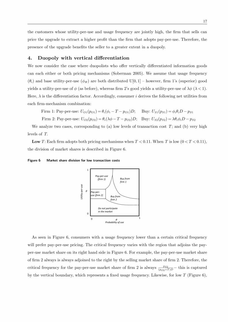
4. Duopoly with vertical differentiation

We now consider the case where duopolists who offer vertically differentiated information goods

can each either or both pricing mechanisms (Soberman 2005). We assume that usage frequency

(θi) and base utility-per-use (φH) are both distributed U[0,1] – however, firm 1’s (superior) good

yields a utility-per-use of φ (as before), whereas firm 2’s good yields a utility-per-use of λφ (λ< 1).

Here, λ is the differentiation factor. Accordingly, consumer i derives the following net utilities from

each firm-mechanism combination:

Firm 1: Pay-per-use: UO1(pO1) = θi(φi−T − pO1)D; Buy: US1(pS1) = φiθiD− pS1

Firm 2: Pay-per-use: UO2(pO2) = θi(λφ−T − pO2)D; Buy: US2(pS2) = λθiφiD− pS2

We analyze two cases, corresponding to (a) low levels of transaction cost T ; and (b) very high

levels of T.

Low T : Each firm adopts both pricing mechanisms when T < 0.11. When T is low (0<T < 0.11),

the division of market shares is described in Figure 6.

Figure 6 Market share division for low transaction costs

θ

φ

10

0

1

Uti

lity

-pe

r-u

se

Probability of use

Buy from

firm 1

Buy from

firm 2

Pay-per-use

(firm 1)

Pay-per-

use (firm 2)

Do not participate

in the market

As seen in Figure 6, consumers with a usage frequency lower than a certain critical frequency

will prefer pay-per-use pricing. The critical frequency varies with the region that adjoins the pay-

per-use market share on its right hand side in Figure 6. For example, the pay-per-use market share

of firm 2 always is always adjoined to the right by the selling market share of firm 2. Therefore, the

critical frequency for the pay-per-use market share of firm 2 is always pS2(pO2+T )D

− this is captured

by the vertical boundary, which represents a fixed usage frequency. Likewise, for low T (Figure 6),

18

the pay-per-use market share of firm 1 is adjoined to the right by the selling market share of firm

1 for high levels of usage utility φ− here again, the critical frequency is pS1(pO1+T )D

, which is again

represented by a vertical boundary. However, for lower values of φ in Figure 6, the pay-per-use

market share of firm 1 is adjoined by the selling market share of firm 2. To find the critical frequency

in these regions, we set UO1(pO1) = US2(pS2). The critical frequency here is θi = pS2[pO1+T−(1−λ)φi]D

.

Intuitively, this frequency is now additionally a function of λ and utility-per-use (φ) because the

competing goods yield different levels of utility.

Analytical expressions for the market shares and profits are derived in Electronic Appendix 11.

We numerically characterize the Nash equilibria. The equilibrium profits are plotted for different

values of T (0< T < 0.11, representing low transaction costs) in Figure 7 and for different values

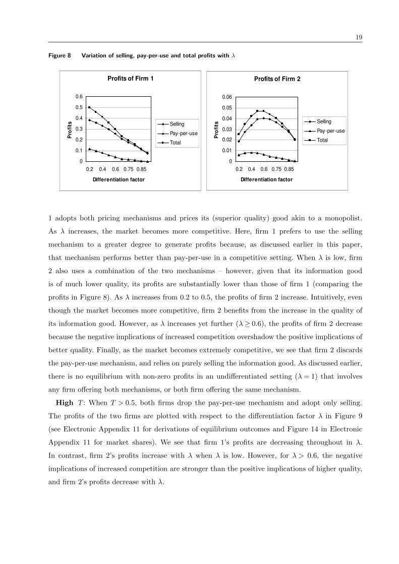
of the differentiation factor λ in Figure 8.

Figure 7 Variation of selling, pay-per-use and total profits with T

Profits of Firm 1

0

0.02

0.04

0.06

0.08

0.1

0.01 0.03 0.05 0.1 0.11

Transaction cost T

Pro

fits

Selling

Pay-per-

use

Total

Profits of Firm 2

0

0.005

0.01

0.015

0.02

0.025

0.01 0.03 0.05 0.1 0.11

Transaction cost T

Pro

fits

Selling

Pay-per-

use

Total

The analysis yields some interesting insights. First, the profits in Figure 7 correspond to the

case where the market is competitive (λ= 0.9) and T is low – the configuration of market shares

corresponds to Figure 6. Here, each firm uses both pricing mechanisms, but the profits from selling

to each firm are much higher than those from pay-per-use. This effect is more pronounced as T

increases because the profits from pay-per-use decrease in T . In particular, the profits from the

pay-per-use mechanism for firm 2, that offers lower quality, are marginal. Therefore, as T increases,

we can expect the firms, and firm 2 in particular, to discard the pay-per-use mechanism.

Moving to Figure 8, we observe that firm 1’s profits from both selling and pay-per-use are

uniformly decreasing in λ. When λ is low, the firms are sufficiently differentiated. Therefore, firm

19

Figure 8 Variation of selling, pay-per-use and total profits with λ

Profits of Firm 1

0

0.1

0.2

0.3

0.4

0.5

0.6

0.2 0.4 0.6 0.75 0.85

Differentiation factor

Pro

fits Selling

Pay-per-use

Total

Profits of Firm 2

0

0.01

0.02

0.03

0.04

0.05

0.06

0.2 0.4 0.6 0.75 0.85

Differentiation factor

Pro

fits

Selling

Pay-per-use

Total

1 adopts both pricing mechanisms and prices its (superior quality) good akin to a monopolist.

As λ increases, the market becomes more competitive. Here, firm 1 prefers to use the selling

mechanism to a greater degree to generate profits because, as discussed earlier in this paper,

that mechanism performs better than pay-per-use in a competitive setting. When λ is low, firm

2 also uses a combination of the two mechanisms – however, given that its information good

is of much lower quality, its profits are substantially lower than those of firm 1 (comparing the

profits in Figure 8). As λ increases from 0.2 to 0.5, the profits of firm 2 increase. Intuitively, even

though the market becomes more competitive, firm 2 benefits from the increase in the quality of

its information good. However, as λ increases yet further (λ≥ 0.6), the profits of firm 2 decrease

because the negative implications of increased competition overshadow the positive implications of

better quality. Finally, as the market becomes extremely competitive, we see that firm 2 discards

the pay-per-use mechanism, and relies on purely selling the information good. As discussed earlier,

there is no equilibrium with non-zero profits in an undifferentiated setting (λ = 1) that involves

any firm offering both mechanisms, or both firm offering the same mechanism.

High T : When T > 0.5, both firms drop the pay-per-use mechanism and adopt only selling.

The profits of the two firms are plotted with respect to the differentiation factor λ in Figure 9

(see Electronic Appendix 11 for derivations of equilibrium outcomes and Figure 14 in Electronic

Appendix 11 for market shares). We see that firm 1’s profits are decreasing throughout in λ.

In contrast, firm 2’s profits increase with λ when λ is low. However, for λ > 0.6, the negative

implications of increased competition are stronger than the positive implications of higher quality,

and firm 2’s profits decrease with λ.

20

Figure 9 Variation of selling, pay-per-use and total profits with λ for very high T

Profits of Firm 1

0

0.07

0.14

0.21

0.28

0.35

0.42

0.4 0.6 0.8

Differentiation factor

Se

llin

g p

rofi

ts

Firm 1

Profits of Firm 2

0

0.01

0.02

0.03

0.04

0.05

0.06

0.4 0.6 0.8

Differentiation factor

Se

llin

g p

rofi

ts

Firm 2

Overall, our findings in this section highlight the importance of thinking about how the pay-

per-use and selling mechanisms can work in cooperation with each other to enhance profits, and

competitively against each other to reduce profits. The optimal go-to-market strategy should bal-

ance these forces with the objective of maximizing firm-level profits.

5. Model extensions and tests for robustness

We extended the model in multiple directions and also tested our findings for robustness:

Variability in usage frequency and utility-per-use: We find that variability in usage fre-

quency does not affect the relative performance of the two mechanisms (Electronic Appendix 12).

If the utility-per-use is higher later in the horizon, the profits under pay-per-use rise more sharply

as the pay-per-use mechanism differentiates perfectly between consumers on the utility-per-use

dimension. Therefore, such an increase in the utility-per-use increases the attractiveness of the

pay-per-use mechanism. However, when the utility-per-use decreases later in the horizon, the mar-

ket share under pay-per-use decreases sharply because the firm is forced to choose a substantially

lower payment-per-use later in the horizon.

Inclusion of implementation and service costs: In an enterprise software context, we

assume that when a software application is purchased outright, an enterprise client incurs a one-

time implementation cost (C) and a service (or maintenance) cost each time the application is

used (cs) (Electronic Appendix 13). Under pay-per-use, the service provider incurs a one-time

implementation cost (S) to move the enterprise client’s database to the service provider’s server,

21

and a service cost (co) each time the client uses the application. As might be expected, an increase

in C and cs favors pay-per-use whereas an increase in S and co favors selling, which is similar to

Ma and Seidmann (2007). Effectively, implementation and service costs shift the boundary that

demarcates the parametric regions where one pricing mechanism yields higher profits than the

other.

Correlated utility dimensions: Modifying the assumption that utility-per-use and usage

frequency are independently distributed, we analyzed the case where these dimensions are perfectly

correlated, so that consumers with high utility-per-use also have a high usage frequency (Electronic

Appendix 14). We find that such correlation further enhances the relative advantage of the pay-

per-use mechanism in a monopoly context. This is because the market share of the pay-per-use

mechanism generally consists of consumers with a high utility-per-use. If these consumers also have

a high usage frequency, the revenue streams that accrue to this mechanism are of even greater

magnitude. The reverse is true in a duopoly with undifferentiated information goods. Intuitively,

under competition, the market share carved out by the selling mechanism consists of consumers

whose utility-per-use and usage utility are both relatively high even when these utility dimensions

are independently distributed. However, when these dimensions are perfectly correlated, selling

efficiently captures the most valuable part of the market. Therefore, such correlation enhances the

relative advantage of selling over pay-per-use in the competitive context.

Non-uniform distributions of utility-per-use and usage frequency: We modified the

assumption that utility-per-use and usage frequency were uniformly distributed (Electronic

Appendix 15). Consider the case where each pricing mechanism is independently used by the

monopolist. First, if utility-per-use has an upper triangular distribution (skewed to the right), we

find that the pay-per-use mechanism does better than in the uniform distribution case. Intuitively,

the market share of the pay-per-use mechanism is graduated solely on the utility-per-use dimension

– therefore, this mechanism can efficiently capture consumers with a high utility-per-use. Selling,

on the other hand, does not benefit as strongly under this distribution because it does not serve

consumers with a low usage frequency, even if their utility-per-use is high. Conversely, if utility-

per-use has a lower triangular distribution (skewed to the left), then the selling mechanism does

better than in the uniform distribution case. This is because the scarcity of consumers with high

utility-per-use hurts the pay-per-use mechanism.

Next, consider the case where usage frequency has an upper triangular distribution (skewed to

the right). Here, we find that, while both mechanisms yield a higher profit than in the uniform dis-

tribution case, selling benefits to a greater extent. This is because selling captures more consumers

22

with both a higher utility-per-use and a higher usage frequency. In contrast, some consumers with a

high utility-per-use who are captured by pay-per-use now use the information good less frequently.

Finally, consider the case where usage frequency has a lower triangular distribution (skewed to the

left). Here, the profits from both mechanisms decrease compared to the uniform distribution case,

but the profits from selling decrease more sharply. This is because selling would ideally capture

customers with both a high utility-per-use and a high frequency, but fewer customers now exhibit

both these characteristics.

Endogenous usage frequency: Finally, we analyzed the case where consumers (endogenously)

reduced their usage frequency if the payment-per-use was high in a setting where a monopolist

chose one of the two mechanisms (Electronic Appendix 16). Here, we find that the monopolist

who adopts pay-per-use lowers the payment-per-period to accommodate this externality. Therefore,

ceteris paribus, selling becomes more attractive in the presence of such endogeneity.

6. Conclusion

We analyzed two pricing mechanisms for information goods – selling, where an up-front payment

bestows unrestricted usage rights, and pay-per-use, where payments are closely tailored to the

consumer’s usage patterns. Consumer utility was modeled as a function of the usage frequency and

the utility-per-use of the good.

We first considered a monopolist who could employ either mechanism. Here, we first showed that

as long as the transaction cost associated with pay-per-use is low, profits from that mechanism

are higher than those from selling. Intuitively, pay-per-use pricing achieves perfect discrimination

along the usage frequency dimension by allowing consumers to pay for the good only when it was

used. In contrast, selling is attractive to consumers who have both a relatively high utility-per-use

and a high usage frequency. We then showed that the presence of a positive unit marginal cost

lowers profits from both mechanisms but hurts selling more than pay-per-use. This is because,

under pay-per-use, there is superior resource pooling and a smaller quantity of goods, representing

a lower total marginal cost, can be more intensively used by multiple customers across time to

satisfy market demand.

Next, we considered the impact of uncertainty in consumer utility-per-use and usage frequency.

We demonstrate that pay-per-use performs relatively well when usage frequency is uncertain. Going

further, we demonstrate that uncertainty in utility-per-use lowers profits from both mechanisms,

but lowers profits from pay-per-use to a greater. This is because the market share of the pay-

per-use mechanism is determined solely based on the distribution of utility-per-use, whereas the

23

reduction in the profits from selling is tempered by the fact that the distribution of usage frequency

is known with certainty. If both the usage frequency and the utility-per-use are uncertain, then

profits under pay-per-use reduce to a lower extent than under selling compared to the case where

both are known with certainty because pay-per-use is not affected by uncertainty along the usage

frequency dimension.

Moving to the competitive context, we analyzed a duopoly where firms offering identical infor-

mation goods could employ either or both pricing mechanisms. We find that, in equilibrium, one

firm adopts selling and the competitor adopts pay-per-use. Here, in contrast to the monopoly, the

seller’s profits generally dominate the pay-per-use provider’s profits. The key implication is that

a monopolist who employs one pricing mechanism is better off with pay-per-use pricing provided

the associated transaction costs are not too high. In contrast, a monopolist who expects future

competition should pursue a “defensive” positioning strategy and choose to sell the good instead.

We also find that the profits of the pay-per-use provider were inverted U-shaped with respect to

the transaction cost associated with that mechanism. The intuition was traced back to the role of

the transaction cost in moderating the level of competition in the market.

We then analyzed a duopoly where firms offering vertically differentiated information goods could

employ either or both pricing mechanisms. When the transaction costs associated with pay-per-use

are low, we find that each firm adopts both mechanisms, but the major share of the profits for each

firm accrues from selling. Whereas the pay-per-use mechanisms contributes only weakly to profits,

the high payments-per-use play a role in propping up the selling prices and increasing profits from

selling. The profits of the firm offering the superior information good are strictly decreasing in the

quality of the competitor. In contrast, the profits of the firm offering the inferior information good

are inverted U-shaped in the quality of the good – the initial improvement in quality increases

profits, but as the separation between the two competing goods decreases, further improvement

in quality depresses profits on account of more intense competition. When the transaction cost

associated with pay-per-use is high, the firm offering the inferior good dispenses with pay-per-use

pricing and adopts only selling, whereas the competitor adopts both mechanisms. This reduces the

intensity of competition and increases the profits of both firms. Finally, when the transaction cost

is very high, both firms adopt only selling. Overall, our findings provide a range of insights into

how pricing strategies for information goods must be designed in various market environments.

Our analysis has the following limitations that can be addressed by future research. First, the

role of usage frequency-based discounts and other price discrimination mechanisms can be analyzed

in both the monopoly and competitive contexts. Second, we have primarily focused on the case

24

where consumers are differentiated in terms of utility-per-use and usage frequency. Future work

could incorporate the notion of horizontal differentiation where consumers have varying preferences

for the offerings. This is an emerging research domain and much remains to be done. We hope our

analysis and findings catalyze further inquiry in the area.

References

Altinkemer, K. and S. Bandyopadhyay. 2000. The effect of the Internet on the music industry.

Journal of Organizational Computing and Electronic Commerce 10 (3) 209224.

Altinkemer, K. and K. Tomak. 2001. A distributed allocation mechanism for network resources

using software agents. Information Technology and Management, 2, 165-173.

Altman, J. and K. Chu. 2001. How to charge for network services – Flat-Rate or Usage-Based.

Computer Networks, 36, 519-531.

Ba, S. and W.C. Johansson. 2006. An exploratory study of the impact of e-service process on

online customer satisfaction. Production and Operations Management. In press.

Bhaskaran, S.R. and S.M. Gilbert. 2005. Selling and leasing strategies for durable goods with

complementary products. Management Science, 51, 1278-1290.

Bhaskaran, S.R. and S.M. Gilbert. 2009. Implications of channel structure for selling and leasing

of durable goods. Marketing Science, Sep/Oct 28, 918-934.

Bonasia, J. 2007. Lawson wary of hype in pay-per-use software. Investors Business Daily, Thurs-

day, August 9.

Bucovetsky, S. and J. Chilton. 1986. Concurrent renting and selling in a durable goods monopoly

under threat of entry. Rand Journal of Economics. 17 261-275.

Bulow, J.I. 1982. Durable-Goods Monopolists. Journal of Political Economy, 90 314-332.

Chavez, C. 2011. T-Mobile Adding New Pay-Per-Use Data to All Smartphone Accounts Without

a Data Plan. Phandroid Newsletter, August 25, 1-2.

Chen, Y., C. Narasimhan and Z.J. Zhang. 2001. Consumer Heterogeneity and Competitive Price-

Matching Guarantees. Marketing Science, 20 (3) 300-314.

Cheng, H.K., H. Demirkan and G.J. Koehler. 2003. Price and capacity competition of application

services duopoly. Information Systems and E-Business Management, 1, 305-329.

Chien, H-K. and C.Y.C. Chu. 2008. Sale or lease? Durable-goods monopoly with network effects.

Marketing Science, Nov/Dec 27, 1012-1019.

Choudhary, V., K. Tomak and A. Chaturvedi. 1998. Economic benefits of renting software.

Journal of Organizational Computing and Electronic Commerce, 8(4), 277-305.

25

Choudhary, V. 2007. Comparison of software quality under perpetual licensing and software as

a service. Journal of Management Information Systems, 24 141-165.

Clark, J. 2011. Hitachi Data Systems gets into rentable clouds. ZDNET UK Newsletter, October

25, 3-3.

Corey, E.R. 1991. Industrial Marketing: Cases and concepts. Prentice-Hall College Division,

March.

Coughlan, A.T. 1985. Competition and cooperation in marketing channel choice: Theory and

application. Marketing Science, Spring, 4 110-129.

Desai, P., O. Koenigsberg and D. Purohit. 2007. The role of production lead time and demand

uncertainty in marketing durable goods. Management Science, 53 150-158.

Desai, P. and D. Purohit. 1998. Leasing and Selling: Optimal Marketing Strategies for a Durable

Goods Firm. Management Science, 44 S19-S34.

Desai, P. and D. Purohit. 1999. Competition in durable goods markets: the strategic consequences

of leasing and selling. Marketing Science, Winter 18, 42-58.

Dewan, R., B. Jing and A. Seidmann. 2003. Product customization and price competition on

the Internet. Management Science, 49, 1055-1070.

Essegaier, S., S. Gupta and Z. J. Zhang. 2002. Pricing Access Services. Marketing Science 21(2)

139-159.

Fishburn, P.C. and A.M. Odlyzko. 1999. Competitive pricing of information goods: Subscription

pricing versus pay-per-use. Economic Theory, 13 (2) 447-470.

Gupta, S. and R. Loulou. 1998. Process innovation, product differentiation, and channel struc-

ture: Strategic incentives in a duopoly. Marketing Science, Fall, 17 301-316.

Gurnani H. and K. Karlapalem. 2001. Optimal Pricing Strategies for Internet-Based Software

Dissemination. The Journal of the Operational Research Society 52 64-70.

Jain, S. and P. Kannan. 2002. Pricing of information products on online servers: Issues, models

and analysis. Management Science, 48, 1123-1142.

Jiang, B., P.Y. Chen and T. Mukhopadhyay. (2007a). Software Licensing: Pay-per-use versus

Perpetual. Tepper School of Business Working Paper, Carnegie-Mellon University.

Jiang, B., P.Y. Chen and T. Mukhopadhyay. (2007b). Pay-per-use enterprise software: the soft-

ware as a service model. Tepper School of Business Working Paper, Carnegie-Mellon University.

Krause, J. 2004. Enhanced TV. The Internet Encyclopaedia, Vol. 2, H. Bidgoli, ed., John Wiley

and Sons.

26

Ma, D. and A. Seidmann. 2007. ASP On-Demand Versus MOTS In-House Software Solutions.

Available at SSRN: http://ssrn.com/abstract=996774

Machine Design. 2000. Renting CAD over the Internet. Machine Design, 72, 70-73.

Machrone, B. 2006. What’s in your wallet? PC Magazine, June 6, 68-69.

McKnight, L. and J. Boroumand. 2000. Pricing Internet services: After flat rate. Telecommuni-

cations Policy, 24, 565-590.

Nault, B. R. and A. S. Dexter. 1995. Added value and pricing with information technology. MIS

Quarterly, 19 (4), 449-463.

Nicolle, L. 2002. At your service. Enterprise, April/May 17-18.

Padmanabhan, V., S. Rajiv and K. Srinivasan. 1997. New Products, Upgrades, and New Releases:

A Rationale for Sequential Product Introduction. Journal of Marketing Research, 34 (4) 456-472.

Postmus, D., J. Wijngaard and H. Wortmann. 2009. An economic model to compare the prof-

itability of pay-per-use and fixed-fee licensing. Information and Software Technology, 51 581-588.

Purohit, D. 1997. Dual distribution channels: the competition between rental agencies and deal-

ers. Marketing Science, Summer 16, 228-245.

Reeve, R. 2011. Enhance Your Productivity via the Web. PC World, October 31, 1-2.

Roush, M. 2011. Altair Enables Innovation in the Cloud by Launching HyperWorks On-Demand.

CBS Detroit Newsletter, June 23.

Sankaranaryan, R. 2007. Innovation and the durable goods monopolist: The optimality of fre-

quent new-version releases. Marketing Science, Nov/Dec, 26, 774-791.

Shulman, J.D. and A.T. Coughlan. 2007. Used goods, not used bads: Profitable secondary market

sales for a durable goods channel. Quantitative Marketing and Economics, 5 (2) 191-210.

Soberman, D. 2005. Questioning Conventional Wisdom About Competition in Differentiated

Markets. Quantitative Marketing and Economics, 3 (1) 41-70.

Sundararajan, A. 2004. Nolinear pricing of information goods. Management Science, 50 1660-

1673.

Train, K. 1991. Optimal regulation. MIT Press, Cambridge, MA.

Varian, H. R. 2000. Buying, sharing and renting information goods. The Journal of Industrial

Economics, XLVIII 4, 473-488..

Yin, S., S. Ray, H. Gurnani and A. Animesh. 2010. Durable products with multiple used goods

markets: Product upgrade and retail pricing implications. Marketing Science, May/Jun, 29 540-560.

Zhang, J. and A. Seidmann. 2003. The optimal software licensing policy under quality uncer-

tainty. Proceedings of the 5th International Conference on Electronic Commerce, ACM Press, New

York, 276-286.

27

Zhang, J. and A. Seidmann. 2010. Selling or Subscribing Software under Quality Uncertainty and

Network Externality Effect. Proceedings of the 43rd Hawaii International Conference on System

Sciences (HICSS), 1-10.

APPENDIX

APPENDIX A1: Proof of Proposition 1:

If the firm charges a payment-per-use of pO, all consumers with φi ≥ pO +T use the information

good. The market fraction using the good is, therefore: φH−(pO+T )

φH. The average frequency of use

for consumers in this fraction in any given period is θH2. The expected profits for the firm are:

ΠO = φH−(pO+T )

φH

θH2pOD

The first order condition (FOC, henceforth) with respect to pO yields pO = φH−T2

. The second

order condition (SOC, henceforth) for ΠO to be concave can easily be seen to be satisfied because

ΠO is quadratic in pO with a negative sign on the square term (the second derivative of ΠO with

respect to pO is −1). Substituting the optimal value for pO in the expression for the market fraction

and profits yields the optimal outcomes.

Under selling, if the firm sets a selling price of pS, then in Figure 2, at any given usage utility

φ,consumers with usage frequencies in the range θ ∈ [ pSφD, θH ] derive (weakly) positive utility from

the purchase. From Figure 1, the market fraction thay buys the good and the profits, respectively,

are denoted by:

MSS = 1φHθH

∫ θHpSφHD

[φH − pSθD

]dθ= 1φHθH

[θHφH − pSD

+ pSD

log{ pSθHφHD

}]

ΠS = pSφHθH

[θHφH − pSD

+ pSD

log{ pSθHφHD

}]

The FOC with respect to pS yields 2pSθHφHD

log{ pSθHφHD

} − pSθHφHD

+ 1 = 0. If pSθHφHD

= d, then

d= 0.285, and therefore pS = 0.285θHφHD. The SOC evaluated at pS = 0.285θHφHD reveals that

the second derivative with respect to pS is negative. For all conditions of pO and pS in all the

sections in this paper, the FOCs are sufficient because the optimal solutions have to be interior

point solutions (except for the monopoly case, where the firm may prefer one mechanism to the

other). This is because the profits go to zero if pO and pS are priced at the extremities (if either pO

or pS is zero, then the margins are zero, and if they are equal to the upper bounds, then the market

shares are zero). Substituting the optimal value for pS in the expression for the market fraction

and profits yields the optimal outcomes. Equating the profits from pay-per-use pricing and selling

yields the cut-off transaction cost.

Social Welfare: We first integrate the cumulative surplus of all consumers who use the infor-

mation good by pay-per-use (consumers with φi > p∗O +T ).

28

Pay-per-use: CS(p∗O) = 1θHφH

∫ φHp∗O

+T(φ−T − p∗O)dφ

∫ θH0

θdθD

= 1φH

(φH−T )2

16θHD since p∗O = φH−T

2.

From Equation (2), if the monopolost uses the selling mechanism, consumer i’s cumulative surplus

is given by:

Selling: UiS(pS) = θiφiD− pSWe next integrate the cumulative surplus of all consumers who buy the information good (con-

sumers with θiφiD > p∗S = 0.285θHφH). For consumers with a given θ, the surplus is given by∫ φH0.285θHφH

θ

(θφ − θHφH)Ddφ. The frequency of usage varies from 0.285θH (when φ = φH) to θH .

Hence,

CS(p∗S) = 1θHφH

[∫ θH

0.285θH{∫ φH

0.285θHφHθ

(θφD− p∗S)dφ}dθ]

= 0.0769θHφHD.

The social welfare is given by the sum of the profits and net consumer surplus from that mech-

anism. �

ELECTRONIC APPENDIX FOR

Pricing Information Goods: A Strategic Analysis of the Selling and Pay-per-use

Mechanisms

ELECTRONIC APPENDIX 1: Joint use of pay-per-use and selling mechanisms in

a monopoly:

Recall that the utilities related to pay-per-use pricing and buying are UiO(pO) = θi(φi−T −pO)D

and UiS(pS) = θiφiD− pS respectively. Consumer i uses pay-per-use only if UiO(pO)> UiS(pS), if

their usage frequency is higher than a critical frequency θc = pS(pO+T )D

. Others will prefer pay-per-

use, or not participate in the market. From Figure 2, the analytical expressions for the market

shares of the selling and pay-per-use mechanisms are the same as in the duopoly, given by:

MSS(pS, pO) = 1φHθH

[∫ θH

pSφHD

[φH − pSθD

]dθ−∫ pS

(pO+T )DpSφHD

[φH − pSθD

]dθ]

= 1φHθH

[θHφH − pSφH(pO+T )D

+ pSD

log{ pSθH (pO+T )D

}]

MSO(pS, pO) = 1φHθH

[φH − (pO +T )] pS(pO+T )D

In calculating MSS(pS, pO) above, we subtract out those consumers with a usage frequency lower

than θc from the market share of selling in the monopoly case. The profits from the selling and

pay-per-use mechanisms, and total profits are, respectively:

ΠS(pS, pO) = 1φHθH

[θHφH − pSφH(pO+T )D

+ pSD

log{ pSθH (pO+T )D

}]pSΠO(pS, pO) = 1

2φHθH[φH − (pO +T )][ pS

(pO+T )D]2pOD

Π(pS, pO) = 1φHθH

[θHφH − pSφH(pO+T )D

+ pSD

log{ pSθH (pO+T )D

}]pS + 12φHθH

[φH − (pO +T )][ pS(pO+T )D

]2pOD

29

Here, the profits corresponding to pay-per-use are computed by multiplying the market share

for pay-per-use pricing and the total payments discounted over time with the average frequency of

usage, given by pS2(pO+T )D

. The analytical expressions for the optimal selling price and the payment-

per-use are derived from the FOCs of Π(pS, pO) with respect to pS and pO. The optimal payment-

per-period derived from the FOCs is: pO = 14[φH − T +

√(φH −T )2 + 16φHT ]− T. Further, from

the FOCs, the optimal selling price satisfies the following implicit equation: θHφH − pS(φH−T )

(pO+T )D+

2pSD

log[ pS(pO+T )θHD

]− pSφHT

(pO+T )2D= 0. After substituting the closed form expression for pO, this implicit

equation can be solved to yield the optimal price for any given set of parameters θH and φH .

Figure 10 Profits from joint use of sellng and pay-per-use in a monopoly

φΗ

θH

0

Pay-per-use

fraction

Uncovered

market

pO+T

Buying

fraction

θc=pS/(pO+T)D

Figure 10 describes the monopolist’s profits from using both mechanisms jointly (assuming θH =

φH = 1, D= 5). The optimal payment-per-period and the optimal price increase from the base case

where the monopolist uses each mechanism alone. It can be verified that the monopolist obtains a

lower market share from each mechanism compared to when each is used independently. However,

the total market share is higher when the mechanisms are used jointly than when each is used

independently. Further, even when both mechanisms are available, the monopolist uses pay-per-

use pricing alone when transaction cost T=0, both mechanisms when T is at a moderate level

(with a substantial fraction of the total profit accruing from pay-per-use pricing), and the selling

mechanism alone when T is high. �

ELECTRONIC APPENDIX 2: Analysis with positive unit variable cost:

As before, the market fraction that participates under pay-per-use pricing is φH−(pO+T )

φH. The

average frequency with which consumers use pay-per-use pricing in any given period is θH2

. The

expected profits for the firm are ΠO = φH−(pO+T )

φH

θH2

(pOD− c). To explain this profit function, note

that the market share is multiplied by the average frequency of usage of θH2

to yield the total

number of times the good is used in any given period. The resulting quantity is then multiplied

30

by pO to yield the total revenue per period. Finally, multiplying the revenue by the NPV discount

factor D yields the discounted value of total revenues. On the cost side, the firm needs to produce

at the outset the quantity of goods that will be used during each period – this is denoted by

φH−(pO+T )

φH

θH2

– at the cost of c per unit. For example, at a video store, a fixed number of DVDs

are procured, which can be used over multiple months. This cost is subtracted from the revenues

to yield the net profits in the expression above. Alternatively, if the firm sells the good outright,

then from eqn (4), the profits are:

ΠS = (pS−c)φHθH

[θHφH − pSD

+ pSD

log( pSθHφHD

)]

The optimal payments per period and the optimal selling price are derived from the correspond-

ing FOCs. The optimal per-period payment is pO = (φH−T )D+c

2and the corresponding profits are

ΠO = [(φH−T )D−c]2θH8φHD

. The optimal price is characterized by the implicit equation θHφH − pSD

+

2pSD

log( pSθHφHD

)− cD

log( pSθHφHD

) = 0.

Both the optimal per-period payment and the optimal price increase if there is a positive unit

variable cost. This is intuitive. The cut-off transaction cost below which pay-per-use pricing yields

higher profits than selling is described in the figure in Figure 11 (for D= 5).

Figure 11 Cut-off transaction cost ratio TCφH

with unit variable cost c (D= 5)

0

0.05

0.1

0.15

0.2

0.1 0.2 0.3 0.4 0.5 0.6 0.7 0.8 0.9

Unit variable cost c

TC/ φφ φφ

H

As observed in Figure 11, the cut-off transaction cost (TC) increases in the unit variable cost.

That is, the presence of a positive unit variable cost increases the relative attractiveness of pay-

per-use compared to selling. �

31

ELECTRONIC APPENDIX 3A

Proof of Proposition 2a:

If the firm adopts the selling mechanism and sets a selling price of pS, the market share of the

firm is:

MS+(pS) = 1φH (θH+v)

[(θH + v)φH − pSD

+ pSD

log( pS(θH+v)φHD

)] if the actual frequency of usage

θ˜U(0, θH + v).

MS−(pS) = 1φH (θH−v)

[(θH − v)φH − pSD

+ pSD

log( pS(θH−v)φHD

)] if the actual frequency of usage

θ˜U(0, θH − v).

The expected profits of the firm are:

E[ΠS(pS)] = pSMS+(pS)+MS−(pS)

2

If the firm adopts pay-per-use and sets a payment-per-use of pO, its profits are:

ΠO+(pO) = φH−(pO+T )

φH

(θH+v)

2pOD if the actual frequency of usage θ˜U(0, θH + v).

ΠO−(pO) = φH−(pO+T )

φH

(θH−v)

2pOD if the actual frequency of usage θ˜U(0, θH − v).

The expected profits of the firm are E[ΠO(pO)] =ΠO+(pO)+ΠO−(pO)

2.

If the firm uses pay-per-use in the presence of uncertainty in usage frequency, its expected profits

are:

E[ΠO(pO)] =ΠO+(pO)+ΠO−(pO)

2=⇒E[ΠO+(pO)] = φH−(pO+T )

φH

(θH+v)

2pOD, which is the same as the

case where the distribution of the frequency of usage is known with certainty. Therefore, the firm

sets the payment-per-use pO = φH−T2

and optimal profits are E[ΠO(pO)] = 18

θH (φH−T )2

φHD.

If the firm adopts selling, its expected profits are:

E[ΠS(pS)] = pSMS+(pS)+MS−(pS)

2where

MS+(pS) = 1φH (θH+v)

[(θH + v)φH − pSD

+ pSD

log( pS(θH+v)φHD

)] and

MS−(pS) = 1φH (θH−v)

[(θH − v)φH − pSD

+ pSD

log( pS(θH−v)φHD

)].

The expected profits under selling are:

E[ΠS(pS)] = pS2

[{1− pSφH (θH+v)D

+ pSφH (θH+v)D

log( pS(θH+v)φHD

)}

+{1− pSφH (θH−v)D

+ pSφH (θH−v)D

log( pS(θH−v)φHD

)}]

In the case without uncertainty, the profits of the firm under selling mechanism are:

ΠS = pS[1− pSθHφHD

+ pSθHφHD

log{ pSθHφHD

}]

We need to show that, when the firm adopts selling, expected profits under uncertainty are lower

than those under no uncertainty. That is, we need to show that:

pS2

[{1− pSφH (θH+v)D

+ pSφH (θH+v)D

log( pS(θH+v)φHD

)}+ {1− pSφH (θH−v)D

+ pSφH (θH−v)D

log( pS(θH−v)φHD

)}]

< pS[1− pSθHφHD

+ pSθHφHD

log{ pSθHφHD

}]

This is true by Jensen’s inequality because for a concave function f , f(x+v)+f(x−v)< 2f(x).

32

Now, to show that f(θH) = pS[1− pSθHφHD

+ pSθHφHD

log{ pSθHφHD

}] is concave in θH ,we note that

∂2f(θH )

∂2θH= pS[−1 + 2 log{ pS

θHφHD}]< 0. This is because pS < θHφHD for selling to be feasible.

Therefore, profits under selling when there is uncertainty in the distribution of usage frequency

are lower than in the absence of uncertainty. Because the profits of the firm under pay-per-use are

identical across the cases with and without uncertainty in usage frequency, the cut-off transaction

cost below which pay-use-use yields higher profits than selling is higher in the presence of such

uncertainty. Stated differently, such uncertainty makes pay-per-use more attractive from the firm’s

perspective. �

ELECTRONIC APPENDIX 3B

Proof of Proposition 2b:

If the firm adopts selling and sets a selling price of pS, its market share is:

MS+(pS) = 1θH (φH+v)

[(φH + v)θH − pSD

+ pSD

log( pS(φH+v)θHD

)] if the utility-per-use φ˜U(0, φH + v)

MS−(pS) = 1θH (φH−v)

[(φH − v)θH − pSD

+ pSD

log( pS(φH−v)θHD

)] if the utility-per-use φ˜U(0, φH − v).

The expected profits are:

E[ΠS(pS)] = pSMS+(pS)+MS−(pS)

2

If the firm adopts pay-per-use and sets a payment-per-use of pO, its profits are

ΠO+(pO) = φH+v−(pO+T )

φH+v

θH2pOD if the actual frequency of usage φ˜U(0, φH + v).

ΠO−(pO) = φH−v−(pO+T )

φH−vθH2pOD if the actual frequency of usage φ˜U(0, φH − v).

The expected profits of the firm are E[ΠO(pO)] =ΠO+(pO)+ΠO−(pO)

2

= [1− pO+T

φH− v2φH

] θH2pOD. Denote φH − v2

φHby φH . Then E[ΠO(pO)] = [1− pO+T

φH] θH

2pOD. The FOC

with respect to pO yields pO = φH−T2

and the expected profits under pay-per-use are E[ΠO(pO)] =

18

θH (φH−T )2

φHD.

Under selling, the expected profits are:

E[ΠS(pS)] =

pS2

[{1− pS(φH+v)θHD

+ pS(φH+v)θHD

log( pS(φH+v)θHD

)}+ {1− pS(φH−v)θHD

+ pS(φH−v)θHD

log( pS(φH−v)θHD

)}]

E[ΠS(pS)] = pS[1− pSθHφHD

+ pSθHφHD

log{ pSθHφHD

}+K] (E2a.1)

where φH = φH − v2

φHand

K = 12[ pS(φH+v)θHD

log( pS(φH+v)θHD

) + pS(φH−v)θHD

log( pS(φH−v)θHD

)]− pSθHφHD

log{ pSθHφHD

}

Condition A1: We show that K > 0 because

pS(φH+v)θHD

log( pS(φH+v)θHD

) + pS(φH−v)θHD

log( pS(φH−v)θHD

)> 2pSθHφHD

log{ pSθHφHD

}

That is, we prove that

pS(φH+v)θHD

log( pSθHD

) + pS(φH+v)θHD

log 1φH+v

+ pS(φH−v)θHD

log( pSθHD

) + pS(φH−v)θHD

log 1φH−v

>

33

2pSθHφHD

log{ pSθHφHD

}

=⇒To prove that

1φH+v

log( pSθHD

) + 1φH+v

log 1φH+v

+ 1φH−v

log( pSθHD

) + 1φH−v

log 1φH−v

> 2

φHlog{ pS

θHD}+ 2

φHlog{ 1

φH}

The terms corresponding to log( pSθHD

) cancel out. Therefore, we need to prove that:

1φH+v

log 1φH+v

+ 1φH−v

log 1φH−v

> 2

φHlog{ 1

φH}

On simplifying, this reduces to proving that

(φH + v) log(φH + v) + (φH − v) log(φH − v)> 2φH logφH

which is true by Jensen’s inequality, because if f is a convex function of x, f(x+v) +f(x−v)>

2f(x). f(φH) = φH logφH is a convex function of φH as ∂2

∂2φH(φH logφH) = 1

φH> 0. Therefore,

Condition A1 is true.

From Equation (E2a.1),

E[ΠS(pS)] = pS[1− pSθHφHD

+ pSθHφHD

log{ pSθHφHD

}+K]

> pS[1− pSθHφHD

+ pSθHφHD

log{ pSθHφHD

}] (E2a.2)

Let pS be the price that maximized the RHS in equation (E2a.2). pS = 0.285θHφHD. Substituting

this back in (E2a.2) gives

E[ΠS(pS)]> 0.1018θHφHD

We have already proved that E[ΠO(pO)] = 18

θH (φH−T )2

φHD. To find the cut-off transaction cost TC

at which the profits from selling and pay-per-use are equal, note that

18

θH (φH−TC)2

φHD > 0.1018θHφHD. Therefore, TC < 0.0976φH = 0.0976(φH − v2

φH),which is lower

than the cutoff transaction cost in the case of no uncertainty (TC = 0.0976 φH). �

ELECTRONIC APPENDIX 3C

Both utility-per-use and usage frequency are uncertain

In this case, we assume that the utility-per-use can be uniform either between 0 and φH + vφ or

uniform between 0 and φH − vφ, with a probability of 0.5 assigned to each of these distributions.

We also assume that usage frequency can be uniform either between 0 and θH + vθ or uniform

between 0 and θH − vθ, with a probability of 0.5 assigned to each of these distributions. This case

cannot be solved in closed form. We numerically simulate and compare profits under the selling

and pay-per-use mechanisms for different values of vφ and vθ (we assume φH = θH = 1), and . The

regions of preference of the selling and pay-per-use mechanisns are described in Figure 12.

ELECTRONIC APPENDIX 4

Proof of Result 1:

Table T1 below summarizes the possible strategies used by both parties in equilibrium.

34

Figure 12 Regions of preference (compared to certainty case) of selling and pay-per-use mechanisms when both

are uncertain

vφ

vθ

Pay-per-use

Sell

x

x x x

xxx

x x x

s

s

s

s

0

φH-T

θH

Firm 1Selling Pay-per-use Both

Selling No equilibrium Equilibrium exists No equilibriumFirm 2 Pay-per-use Equilibrium exists No equilibrium No equilibrium

Both No equilibrium No equilibrium No equilibriumTable T1 : Nash equilibrium outcomes when firms can use either or both mechanisms

Case 1: Firm 1 uses only selling, Firm 2 uses only selling

If the firms each use the selling mechanism only, let the selling price charged by firm 1 be denoted

by pS1 and the selling price of firm 2 be denoted by pS2. Let the profits of firm 1 be denoted by

ΠS1(pS1, pS2) and the profits of firm 2 be denoted by ΠS2(pS1, pS2). A necessary condition for the

Nash equilibrium (with non-zero profits for both firms) to exist is (here p∗S1 and p∗S2 are the Nash

equilibrium prices):

ΠS1(p∗S1, p∗S2)>ΠS1(p∗S1 + ε, p∗S2) and ΠS1(p∗S1, p

∗S2)>ΠS1(p∗S1− ε, p∗S2)

ΠS2(p∗S1, p∗S2)>ΠS2(p∗S1, p

∗S2 + ε) and ΠS2(p∗S1, p

∗S2)>ΠS2(p∗S1, p

∗S2− ε)

That is, both firms should have no incentive to deviate from the Nash equilibrium prices.

The net surpluses of a consumer who buys the information from firm 1 and firm 2 are, respec-

tively:

UiS1(pS1) = θiφiD− pS1

UiS1(pS2) = θiφiD− pS2

If the information good is not vertically differentiated, it is easy to see that if pS1 6= pS2, the

entire market share goes to the firm with the lower selling price, and the other firm is left with

zero profits. This leads to price undercutting, which can be formally proven as follows.

Without loss of generality, assume that the selling price duo (p∗S1, p∗S2) is a Nash equilibrium and

35

let p∗S1 < p∗S2, where p∗S1 > 0 and p∗S2 > 0. Then,

ΠS1(p∗S1, p∗S2) = p∗S1[1− p∗S1

θHφHD+

p∗S1θHφHD

log(p∗S1

θHφHD)]

ΠS2(p∗S1, p∗S2) = 0

However, for firm 2, ΠS2(p∗S1, p∗S2) > ΠS2(p∗S1, p

∗S2 − ε) is not satisfied, because if ε = lim

h→0p∗S2 −

p∗S1−h,then:

ΠS2(p∗S1, p∗S2− ε) = lim

h→0(p∗S1−h)[1− p∗S1−h

θHφHD+

p∗S1−hθHφHD

log(p∗S1−hθHφHD

)]>ΠS2(p∗S1, p∗S2) = 0 for all p∗S1 >

0.

Therefore, there is a contradiction, and a non-zero price Nash equilibrium cannot exist if p∗S1 6=

p∗S2. Since profits are zero if the prices are zero, a non-zero price Nash equilibrium cannot exist if

p∗S1 6= p∗S2.

Now, let us assume that (p∗S1, p∗S2) is a Nash equilibrium and let p∗S1 = p∗S2 = p∗S, where p∗S1 =

p∗S2 > 0. Because the net consumer surplus for both firms is equal, we can assume that the market

shares for both firms are equal (half of that of the monopolist who prices at p∗S). Then:

ΠS1(p∗S1, p∗S2) =

p∗S2

[1− p∗SθHφHD

+p∗S

θHφHDlog(

p∗SθHφHD

)] and

ΠS2(p∗S1, p∗S2) =

p∗S2

[1− p∗SθHφHD

+p∗S

θHφHDlog(

p∗SθHφHD

)]

In this case, the conditions ΠS1(p∗S1, p∗S2)>ΠS1(p∗S1− ε, p∗S2) and ΠS2(p∗S1, p

∗S2)>ΠS2(p∗S1, p

∗S2− ε)

are not satisfied for all p∗S > 0. If ε= limh→0

h, for firm 1, then:

ΠS1(p∗S1− limh→0

h,p∗S2) = limh→0

(p∗S −h)[1− p∗S−hθHφHD

+p∗S−hθHφHD

log(p∗S−hθHφHD

)]

>p∗S2

[1− p∗SθHφHD

+p∗S

θHφHDlog(

p∗SθHφHD

)].

A symmetric condition holds for firm 2. Therefore, there is a contradiction and Nash equilibrium

with non-zero prices and profits exists when each firm employs only selling. �

Case 2: Firm 1 uses only the pay-per-use mechanism and Firm 2 uses only the

pay-per-use mechanism only

Similar to case 1, each firm can undercut the (positive) payment-per-use of other to obtain

the full market share, and therefore, there is no equilibrium where either firm charges a positive

payment-per-use and makes a positive profit in this case. The detailed proof is very similar to Case

1 and can be obtained from the authors. �

Case 3: Firm 1 uses the selling mechanism only, Firm 2 uses the pay-per-use mech-

anism only

This case is analyzed in Electronic Appendix 6 (see below), and it yields an equilibrium with a

positive payment-per-use and a positive selling price, and positive profits for each firm. The case

with firm 1 using pay-per-use only and firm 2 using selling only is symmetric.

36

Case 4: Firm 1 uses the selling and pay-per-use mechanisms together, Firm 2 uses

the pay-per-use mechanism only

Let the payment-per-use charged by firm 1 be denoted by pO1, its selling price by pS1 and the

payment-per-use of firm 2 by pO2. Let the profits of firm 1 be denoted by ΠB1(pS1, pO1, pO2) and

the profits of firm 2 be denoted by ΠO2(pS1, pO1, pO2). The following conditions should hold for a

Nash equilibrium (with non-zero profits to each firm) to exist (here, p∗S1, p∗O1 and p∗O2 are the Nash

equilibrium prices):

ΠB1(p∗S1, p∗O1, p

∗O2)>ΠB1(p∗S1, p

∗O1 + ε, p∗O2) and ΠB1(p∗S1, p

∗O1, p

∗O2)>ΠB1(p∗S1, p

∗O1− ε, p∗O2)

ΠO2(p∗S1, p∗O1, p

∗O2)>ΠO2(p∗S1, p

∗O1, p

∗O2 + ε) and ΠO2(p∗S1, p

∗O1, p

∗O2)>ΠO2(p∗S1, p

∗O1, p

∗O2− ε)

That is, both firms should have no incentive to deviate from the Nash equilibrium prices. The net

consumer surpluses derived from buying from firm 1 or from adopting the pay-per-use mechanism

from firms 1 and 2 are, respectively:

UiS1(pS1) = θiφiD− pS1

UiO1(pO1) = θiD[φi− (pO1 +T )]

UiO1(pO2) = θiD[φi− (pO2 +T )]

Similar to the previous case, we can show that if p∗O1 6= p∗O2, then the firm with the higher

payment-per-use obtains zero market share and can simply discard that pricing mechanism. If that

firm is firm 2, then firm 2 obtains zero profits overall. Therefore, firm 2 has the incentive to reduce

its payment-per-use to a level below that of firm 1. Therefore, no equilibrium is possible with

p∗O1 6= p∗O2, if firm 2 charges the lower payment-per-use. On the other hand, if the firm that with

the higher payment-per use is firm 1, than that mechanism obtains zero market share for firm 1.

In this case, that mechanism can be discarded by firm 1, and we arrive at a situation where firm

1 adopts only selling and firm 2 adopts only pay-per-use (which does constitute an equilibrium).

Now, let us assume that (p∗S1, p∗O1, p

∗O2) is a Nash equilibrium and let p∗O1 = p∗O2 = p∗O, where

p∗O1 = p∗O2 > 0 and p∗S1 > 0. Because the net consumer surplus for both firms from the pay-per-use

mechanism is equal, we can assume that the market share from the pay-per-use mechanism for

both firms is equal. Then,

ΠB1(p∗S1, p∗O1, p

∗O2) =

p∗S1[1− p∗S1φHθHφH (p∗

O+T )D

+p∗S1

θHφHDlog{ p∗S1

θH (p∗O

+T )D}]+ 1

2φHθH[φH − (p∗O +T )][

p∗S1(p∗O

+T )D]2p∗O2D and

ΠO2(p∗S1, p∗O1, p

∗O2) = 1

2φHθH[φH − (p∗O +T )][

p∗S1(p∗O

+T )D]2p∗O2D

In this case, the conditions ΠB1(p∗S1, p∗O1, p

∗O2)> ΠB1(p∗S1, p

∗O1 − ε, p∗O2) and ΠO2(p∗S1, p

∗O1, p

∗O2)>

ΠO2(p∗S1, p∗O1, p

∗O2− ε) are not satisfied for all p∗O > 0. If ε= lim

h→0h, for firm 1,

ΠB1(p∗S1, p∗O1− lim

h→0h,p∗O2) =

37

limh→0

p∗S1[1− p∗S1φHθHφH (p∗

O−h+T )D

+p∗S1

θHφHDlog{ p∗S1

θH (p∗O−h+T )D

}]+ 12φHθH

[φH−(p∗O−h+T )][p∗S1

(p∗O−h+T )D

]2(p∗O−

h)D

>p∗S1[1− p∗S1φHθHφH (p∗

O+T )D

+p∗S1

θHφHDlog{ p∗S1

θH (p∗O

+T )D}]+ 1

2φHθH[φH − (p∗O +T )][

p∗S1(p∗O

+T )D]2p∗O2D.

A symmetric argument holds for firm 2 as well. Intuitively, with equal and positive payments-

per-use across the firms, one firm can always lower its payment-per-use slightly and capture all

the market share associated with the pay-per-use mechanism of the competitor. Therefore, there is

a contradiction and no Nash equilibrium with positive profits for each firm when the pay-per-use

mechanism is offered by both firms. The no-equilibrium outcomes for the other cases (corresponding

to the cells in Table T1) are proved similarly. and the proofs are available with the authors. �

ELECTRONIC APPENDIX 5: Proof of price and payment-per-use in a duopoly

Consider a duopoly where one firm offers pay-per-use and the competitor sells the informa-

tion good. From Figure 2, the expressions for the market shares of the selling and pay-per-use

mechanisms are, respectively:

MSS(pS, pO) = 1φHθH

[∫ θH

pSφHD

(φH − pSθD

)dθ−∫ pS

(pO+T )DpSφHD

(φH − pSθD

)dθ]

= 1φHθH

[θHφH − pSφH(pO+T )D

+ pSD

log{ pSθH (pO+T )D

}]

MSO(pS, pO) = 1φHθH

[φH − (pO +T )] pS(pO+T )D

The competing firms maximize their individual profits:

Seller: MaxpS

ΠS(pS, pO) = 1φHθH

[θHφH − pSφH(pO+T )D

+ pSD

log{ pSθH (pO+T )D

}]pSPay-per-use: Max

pOΠO(pS, pO) = 1

2φHθH[φH − (pO +T )][ pS

(pO+T )D]2pOD

The profits of the firm that offers pay-per-use pricing are:

ΠO = 12φHθH

[φH − (pO +T )][ pS(pO+T )D

]2pOD

The first order condition with respect to pO yields:

(pO +T )2[φH − 2pO−T ] = 2pO[φH − (pO +T )](pO +T )

which on simplification yields pO = T (φH−T )

φH+T. Next, the seller’s profits in the duopoly are:

ΠS = 1φHθH

[θHφH − pSφH(pO+T )D

+ pSD

log{ pSθH (pO+T )D

}]pSThe FOC for the seller with respect to ps yields:

θHφH − 2pSφH(pO+T )D

+ pSD

log{ pSθH (pO+T )D

}+ pSD

[1 + log{ pSθH (pO+T )D

}] = 0

which on simplification yields the implicit equation:

θHφH − 2pSφH(pO+T )D

+ 2pSD

log{ pSθH (pO+T )D

}+ pSD

= 0

ELECTRONIC APPENDIX 6: Proof of Proposition 3

(i) To prove that the equilibrium payment-per-use in the duopoly is lower than the optimal

payment-per-use charged by a monopolist who employs only the pay-per-use mechanism, we need

to prove that T (φH−T )

φH+T≤ φH−T

2, which simplifies to φH ≥ T. This is true by assumption.

38

(ii) Next, consider the selling price. We have to show that the selling price in a duopoly

(referred to in this proof as pDS) as characterized by the implicit equation θHφH − 2pDSφH(pDO+T )D

+

2pDSD

log{ pDSθH (pDO+T )D

} + pDSD

= 0 (where pDO = T (φH−T )

φH+T) is lower than the selling price in a

monopoly (referred to in this proof as pPS) as characterized by the implicit equation θHφH +

2pPSD

log pPS − pPSD

[2 log(DφHθH) + 1] = 0 (where pPS = 0.285θHφHD).

We rewrite the implicit equations for the selling price in the duopoly and monopoly cases as,

respectively:

θHφH + 2pDSD

log pDS − pDSD

[2 log(DθH) + 2 log(pDO +T ) + 2φHpDO+T

− 1] = 0

θHφH + 2pPSD

log pPS − pPSD

[2 log(DφHθH) + 1] = 0

Comparing the two implicit equations, we note that if the part of the third term multiplying

pDSD

in the first equation is greater than the one multiplying pPSD

in the second equation, then the

corresponding pDS must be smaller for the equations to both equal zero. Therefore, to show that

pDS < pPS, we need to show that:

2 log(DθH) + 2 log(pDO +T ) + 2φHpDO+T

− 1> 2 log(DφHθH) + 1

which reduces to showing that 2φHpDO+T

− 1> 2 log φHpDO+T

+ 1

which reduces to showing that φHpDO+T

> log φHpDO+T

+ 1.

Now this is always true because, if x > 1, then x > 1 + log(x), as evident from the power series

expansion of log(x).

(iii) Finally, one can directly see from the expression pO = T (φH−T )

φH+Tthat the equilibrium payment-

per-use first increases and then decreases with T. �

ELECTRONIC APPENDIX 7: Proof of Proposition 4

To prove that the seller’s profits in the duopoly are always greater than those of the firm that

offers pay-per-use pricing, we have to prove that (using expressions from above):

ΠDS = 1φHθH

[θHφH − pDSφH(pDO+T )D

+ pDSD

log{ pDSθH (pDO+T )D

}]pDS >ΠDO =

12φHθH

[φH − (pDO +T )][ pDS(pDO+T )D

]2pDOD

Note that for the selling price in a duopoly, the FOC is given by:

θHφH − pDSφH(pDO+T )D

+ pDSD

log{ pDSθH (pDO+T )D

}= pDSφH(pDO+T )D

− pDSD

log{ pDSθH (pDO+T )D

}− pDSD

Substituting the right hand side into the expression for ΠDS,we have to prove that:

pDS[pDSφHrD

− pDSD

log{ pDSθHrD

}− pDSD

]> 12(r−T )(φH − r)

p2DSr2D

where r= pDO +T = 2TφHφH+T

.

This reduces to proving that φHr− log{ pDS

θHrD}−1> 1

2

(r−T )(φH−r)r2

. After simplification, this reduces

to proving that (φH − r−T )r+φHT − 2r2 log{ pDSθHrD

}> 0 or (φH − r)(r+T )> 2r2 log{ pDSθHrD

}.

Note that φH > r because r= 2TφHφH+T

, and by assumption, T < φH . The term (r+T ) = 3TφH+T2

φH+Tis

positive. Therefore, the LHS is positive. Now, pDSrD

= pDS(pDO+T )D

is the cut-off frequency under which

39

pay-per-use yields the same utility surplus as selling (see Section 3.2 in the paper). Therefore,

pDSrD

< θH and pDSθHrD

< 1. The natural logarithm of a number less than 1 is always negative –

therefore, the RHS is negative. Therefore, (φH − r)(r+T )> 2r2 log{ pDSθHrD

} always holds true. �

ELECTRONIC APPENDIX 8:

Social Welfare:

As proved above in Electronic Appendix 6, the payment-per-use in the duopoly is p∗O = T (φH−T )

φH+T.

The total net consumer surplus from using the pay-per-use is:

1

φHpDS

(p∗O

+T )D

∫ φHp∗O

+T[φ− p∗O +T ]dφ

∫ pDS(p∗O

+T )D

0 θdθD

Here, the maximum frequency of the consumers using the pay-per-use mechanism is given by

pDS(p∗O

+T )D.

Therefore, the net consumer surplus = φH (φH−T )2

4(φH+T )2pDS

(p∗O

+T ).

The total social welfare is the sum of the profits of the firm adopting pay-per-use and the net

consumer surplus from that mechanism.

For selling, we integrate the cumulative surplus of all consumers who buy the information good

(consumers with θiφiD> p∗S = 0.285θHφH and θi >pDS

(p∗O

+T )D). We first find the cumulative surplus

for consumers with a given usage frequency (θ) and then integrate across θ to find the cumulative

net surplus. The total social welfare is the sum of the cumulative surplus and the profits of the

seller. For consumers with a given θ, the net social welfare is∫ φHkθHφH

θ

(θφ − kθHφH)Ddφ, where

pDS = kθHφHD satisfies θHφH − 2pDSφH(pO+T )D

+ 2pDSD

log{ pDSθH (pO+T )D

}+ pDSD

= 0, the implicit solution for

the selling price in a duopoly. The frequency of usage varies from kθH (when φ= φH) to θH .

Hence, net consumer surplus from selling= 1θHφH

[∫ θHkθH{∫ φHkθHφH

θ

(θφD− p∗S)dφ}dθ]

= θHφH4− φH

4θH[ pDS(p∗O

+T )D]2− kφH{θH − pDS

(p∗O

+T )D}− k2θHφH

2log{ pDS

θH (p∗O

+T )D}

The net social welfare, which comprises the sum of the consumer surplus and profits from selling,

is plotted in Figure 13. �

ELECTRONIC APPENDIX 9

Proof of Proposition 5: We first derive the optimal payment-per-use, prices, and profits when

the basic information good is introduced at the outset and an upgrade is introduced in period k.

Pay-per-use pricing: When the information good is first introduced, all consumers with φi >

pO1 + T use the good, where pO1 denotes the payment-per-period for the basic (non-upgraded)

good. Therefore, the market fraction initially using the good is φH−(pO1+T )

φH. The average usage

frequency for consumers in this fraction in any period is θH2

. Between the kth and N th periods (i.e.,

post-upgrade), if the firm charges a per-period payment of pO2, then the market fraction using

40

Figure 13 Net consumer surplus and social welfare of selling and pay-per-use mechanisms in duopoly (θH =

φH = 1, D= 5)

0

0.1

0.2

0.3

0.4

0.5

0.6

0 0.2 0.4 0.6 0.8 1

Transaction cost T

Ne

t c

on

su

me

r s

urp

lus

Selling

Pay-per-use

0

0.1

0.2

0.3

0.4

0.5

0.6

0 0.2 0.4 0.6 0.8 1

Transaction cost T

So

cia

l W

elf

are

Selling

Pay-per-use

the good on demand is aφH−(pO2+T )

aφH. The average usage frequency for consumers in this fraction

in any period is again θH2

. Accordingly, the firm’s profits are ΠO1 = φH−(pO1+T )

φH

θH2pO1Dk−1 for the

first k− 1 periods. For the periods between and including the kth and N th periods, its profits are

ΠO2 = aφH−(pO2+T )

aφH

θH2pO2(D−Dk−1). It can be verified that the total profits (ΠO = ΠO1 + ΠO2) are

quadratic with respect to both pO1 and pO2. Accordingly, the FOCs with respect to each of these

yield the optimal per-period payments: pO1 = φH−T2

and pO2 = aφH−T2

. Substituting them back into

the profit function yields the total profits denoted by ΠO = θH8

[ (φH−T )2

φHDk−1 + (aφH−T )2

aφH(D−Dk−1)]

. It is easy to see that under pay-per-use pricing with myopic consumers, there is no coupling

between the profits before and after the upgrade has been introduced.

Selling: This pertains to the situation where the monopolist sells the information good and

consumers are myopic. Denote the selling price of the basic good by pS and let pU be the price

of the upgrade introduced in period k. There are two classes of consumers here. The first class of

consumers purchase the basic information good at the outset. The second class of consumers, which

is a subset of the first class, purchase the upgrade in period k. Their surpluses are, respectively,

U1(S) = θiφiD− pS and U2(S) = θi(a− 1)φi(D−Dk−1)− δk−1pU . For the basic information good

in the first period, all consumers with usage probability in the range θ ∈ [ pSφD, θH ] derive (weakly)

positive utility from their purchase. Similar to the scenario without the upgrade, the fraction of

the market purchasing the basic good and the resulting profits are, respectively:

MSS1 = 1φHθH

∫ φHφ=

pSθHD

[θH − pSφD

]dφ= 1φHθH

[θHφH − pSD

+ pSD

log( pSθHφHD

)]

ΠS1 =MSS1pS = pSφHθH

[θHφH − pSD

+ pSD

log( pSθHφHD

)].

41

For the upgrade in the kth period, all consumers with usage probability in the range θ ∈

[ δk−1pU(a−1)φi(D−Dk−1)

, θH ] derive (weakly) positive utility from their purchase. The fraction of the market

purchasing and the resulting profits for the upgrade are, respectively:

MSS2 = 1φHθH

∫ φHφ=

δk−1pU(a−1)(D−Dk−1)θH

[θH − δk−1pU(a−1)φ(D−Dk−1)

]dφ=

1φHθH

[θHφH − δk−1pU(a−1)(D−Dk−1)

+ δk−1pU(a−1)(D−Dk−1)

log( δk−1pU(a−1)θHφH (D−Dk−1)

)]

ΠS2 =MSS2δk−1pU = δk−1pU

φHθH[θHφH − δk−1pU

(a−1)(D−Dk−1)+ δk−1pU

(a−1)(D−Dk−1)log( δk−1pU

(a−1)θHφH (D−Dk−1))]

Note that if the firm uses the selling mechanism only, its profits from selling the base information

good are: ΠS1 =MSS1pS = pSφHθH

[θHφH− pSD

+ pSD

log( pSθHφHD

)]. From Proposition 4, these profits are

optimized if pS = 0.285 θH φHD and the firm’s profits from the basic information good are: ΠS1 =

0.1018 θH φHD. From the upgrade, the firm’s profits are: ΠS2 = MSS2δk−1pU = δk−1pU

φHθH[θHφH −

δk−1pU(a−1)(D−Dk−1)

+ δk−1pU(a−1)(D−Dk−1)

log( δk−1pU(a−1)θHφH (D−Dk−1)

)]. The FOC with respect to pU yields:

2δk−1pUθHφH (a−1)(D−Dk−1)

log{ δk−1pUθHφH (a−1)(D−Dk−1)

} − δk−1pUθHφH (a−1)(D−Dk−1)

+ 1 = 0. The solution to this

implicit equation is: δk−1pU = 0.285 θH φH(a− 1)(D−Dk−1). This yields the same market share

for the upgrade as the basic information good, implying that all consumers who purchase the basic

good also purchase the upgrade. Substituting this back into the profit function yields: ΠS2 = 0.1018

θH φH(a− 1)(D−Dk−1). The total profits of the seller from the base information good and the

upgrade are ΠS = ΠS1 + ΠS2 = 0.1018 θH φH [D+ (a− 1)(D−Dk−1)].

Now, if the firm offers an upgrade, then profits under pay-per-use pricing are ΠO =

θH8

[ (φH−T )2

φHDk−1 + (aφH−T )2

aφH(D−Dk−1)] and, as demonstrated above, those under selling are ΠS =

0.1018 θH φH [D + (a− 1)(D −Dk−1)]. To find the cut-off transaction cost in the scenario with

upgrades, we equate these profits:

θH8

[ (φH−TC)2

φHDk−1 + (aφH−TC)2

aφH(D−Dk−1)] = 0.1018 θH φH [D+ (a− 1)(D−Dk−1)]

Therefore, (1− TCφH

)2Dk−1 + (a− TCφH

)2D−Dk−1

a= 0.1018 ∗ 8[D+ (a− 1)(D−Dk−1)]

Rewrite the LHS as (1− TCφH

)2[D+(a−1)(D−Dk−1)]−(1− TCφH

)2[D−Dk−1 +(a−1)(D−Dk−1)]+

(a− TCφH

)2D−Dk−1

a. If the first term is set equal to the RHS, it yields TC = 0.0976 φH , because the

solution to (1− TCφH

)2D = 0.1018 ∗ 8D is TC = 0.0976 φH . We will first show that the sum of the

other two terms on the LHS is positive. To do this, we need to show that:

(a− TCφH

)2D−Dk−1

a> (1− TC

φH)2[D−Dk−1 + (a− 1)(D−Dk−1)]

or to show that (a− TCφH

)2 >a2(1− TCφH

)2

or to show that a− TCφH

>a− aTCφH

.

Now this is true by assumption because a > 1 for the upgrade. Now, given that the sum of the

other two terms is positive, the first term on the LHS has to be lower so that the equality continues

to hold. Therefore, in order to make the term (1− TCφH

)2 smaller, the cut-off transaction cost TC

42

below which pay-per-use is more profitable than selling is higher than it is in the absence of an

upgrade. �

ELECTRONIC APPENDIX 10

Proof of Proposition 6: If consumers are myopic, then when the firms introduce the base

information good, as in the duopoly case in Section 3.2, the profits of the two firms from the base

information good are:

ΠS(pS, pO) = 1φHθH

[θHφH − pSφH(pO+T )D

+ pSD

log{ pSθH (pO+T )D

}]pSΠO(pS, pO) = 1

2φHθH[φH − (pO +T )][ pS

(pO+T )D]2pOD

From Proposition 3, we know that the firm that adopts the selling mechanism has higher profits

from the base information good than the firm that adopts the pay-per-use mechanism. When the

two firms introduce the upgrade, they no longer compete with each other for the upgrade because

consumers have chosen either the pay-per-use mechanism or the selling mechanism for the base

good (under certain conditions that prevent consumers from switching to the other mechanism,

which can be seen to be easily satisfied for the upgrade to yield positive utility to either set of

consumers). Because the market share of the selling mechanism for the base information good is

higher under competition, and because selling has already captured the customers whose utility-

per-use and usage frequency are jointly high, the firm that sells can price the upgrade to extract a

higher profit than the firm that adopts pay-per-use. Therefore, the presence of the upgrade benefits

the seller to a greater extent in a duopoly. �

ELECTRONIC APPENDIX 11:

Market shares and profits under competition with vertical differentiation

We focus on deriving analytical expressions for the firms’ market shares and profits below.

Equilibrium outcomes were then derived after numerically solving the first order conditions corre-

sponding to these profit expressions.

Case 1: Low transaction cost (Figure 6)

When the transaction cost is low (0 < T < 0.11), the equilibrium division of market shares is

displayed in Figure 6 in the paper. On the lower side, the market share of the selling mechanism for

firm 1 is obtained by comparing the net consumer surpluses from buying that good from firm 1 and

buying the good offered by firm 2. Consumers buy the good from firm 1 iff US1(pS1) = φiθiD−pS1 >

US2(pS2) = λθiφiD−pS2 =⇒ φiθi >pS1−pS2(1−λ)D

. On the left, the market share of the selling mechanism

employed by firm 1 is characterized by θi >pS1

(pO1+T )D. Therefore, the market share of that good

from selling is:

43

MSS1 =∫ 1

pS1(pO1+T )D

[1− pS1−pS2(1−λ)θD

]dθ= 1− pS1(pO1+T )D

+ pS1−pS2(1−λ)D

log( pS1(pO1+T )D

)

To find the market share of the pay-per-use mechanism of firm 1, we note that the pay-per-use

market share is to the left of the selling market share of firm 1 above and the selling market share

of firm 2 below. The latter boundary is represented by UO1(pO1) = θi(φi−T − pO1)D=US2(pS2) =

λθiφiD−pS2, which is characterized by θi = pS2[pO1+T−(1−λ)φi]D

. On the right side (above), the market

share is bounded by firm 1’s selling region, and this boundary is characterized by θi = pS1(pO1+T )D

. On

the lower side, the market share of the pay-per-use mechanism of firm 1 is bounded by the market

share of the pay-per-use mechanism of firm 2. This boundary is represented by UO1(pO1) = θi(φi−

T − pO1)D = UO2(pO2) = θi(λφ− T − pO2)D, which is characterized by φi = pO1−pO2(1−λ)

. Integrating

out the relevant area, the market share of the pay-per-use mechanism of firm 1 is:

MSO1 = [1− (pS1−pS2)(pO1+T )

pS1(1−λ)] pS1(pO1+T )D

+∫ (pS1−pS2)(pO1+T )

pS1(1−λ)pO1−pO2

(1−λ)

pS2[pO1+T−(1−λ)φi]D

dφ

= pS1(pO1+T )D

− (pS1−pS2)

(1−λ)D− pS2

(1−λ)Dlog pS2(pO1+T )

pS1(pO2+T )

To find the market share of the pay-per-use mechanism of firm 2, we note that the pay-per-

use market share is to the left of the selling market share of firm 2. The boundary between the

two regions is represented by: UO2(pO2) = θi(λφ− T − pO2)D = US2(pS2) = λθiφiD− pS2, which is

characterized by θi = pS2(pO2+T )D

. On the lower side, the market share of the pay-per-use mechanism

of firm 2 is bounded by zero, and this boundary is characterized by: φi = pO2+T

(1−λ). Therefore, the

market share of the pay-per-use mechanism of firm 2 is:

MSO2 = [pO1−pO2(1−λ)

− pO2+T

(1−λ)] pS2(pO2+T )D

We next find the fraction of non-adopters. This fraction is represented by the area under the

pay-per-use and selling regions of firm 2. The area under the fraction of φi = pO2+T

λwho buy

information good from firm 2 is:∫ pO2+Tλ

pS2λD

[1− pS2λφD

]dφ= pO2+T

λ− pS2

λD+ pS2

λDlog[ pS2

(pO2+T )D]

Therefore, the total fraction of non-adopters is:

MSNA = pO2+T

λ− [pO2+T

λ− pS2

λD+ pS2

λDlog[ pS2

(pO2+T )D] = pS2

λD− pS2

λDlog[ pS2

(pO2+T )D]

The market share of the selling mechanism of firm 2 is: MSS2 = 1−MSS1 −MSO1 −MSO2 −

MSNA

The profits from the pay-per-use mechanism for firm 1 equal the sum of the profits from two

areas: the region bounded by the selling region of firm 1 to the right, and the region bounded by

the selling region of firm 2 to the right. Denoting these profits by ΠO1(RS1) and ΠO1(RS2), we

obtain:

ΠO1(RS1) = [1− (pS1−pS2)(pO1+T )

pS1(1−λ)] 12[ pS1(pO1+T )D

]2pO1D

Here 12

pS2[pO1+T−(1−λ)φi]D

is the average frequency of usage.

44

ΠO1(RS2) = pO1D∫ (pS1−pS2)(pO1+T )

pS1(1−λ)pO1−pO2

(1−λ)

pS2[pO1+T−(1−λ)φi]D

∗ 12

pS2[pO1+T−(1−λ)φi]D

dφ

= pO1p2S2

2D(1−λ)[ pS1pS2(pO1+T )

− 1pO2+T

]

Therefore,

ΠO1(pS1, pO1) = [1− (pS1−pS2)(pO1+T )

pS1(1−λ)] 12[ pS1(pO1+T )D

]2pO1D+ pO1p2S2

2D(1−λ)[ pS1pS2(pO1+T )

− 1pO2+T

]

The profits from the pay-per-use mechanism for firm 2 are:

ΠO2(pS2, pO2) = [pO1−pO2(1−λ)

− pO2+T

(1−λ)] 12[ pS2(pO2+T )D

]2pO2D

The total profits of the two firms are:

Π1(pS1, pO1) = pS1MSS1 + ΠO1(pS1, pO1)

= pS1MSS1 + pO1p2S2

2D(1−λ)[ 1[pO1+T−(1−λ)]

− 1pO2+T

]

Π2(pS2, pO2) = pS2MSS2 + ΠO2(pS2, pO2)

= pS2MSS2 + [pO1−pO2(1−λ)

− pO2+T

(1−λ)] 12[ pS2(pO2+T )D

]2pO2D

Case 2: Very High transaction cost (T > 0.5)

Figure 14 Market shares of firm 1 and firm 2 with very high transaction cost

φΗ

θH

0

Firm 1

Firm 2

When the transaction cost is very high, each firm uses only the selling mechanism. The market

share of firm 1 is bounded below by the market share of firm 2, and is characterized by: φiθi >

pS1−pS2(1−λ)D

. The market shares of firms 1 and 2 are plotted in Figure 14. Therefore, firm 1’s market

share is:

MSS1 =∫ 1pS1−pS2(1−λ)D

[1− pS1−pS2(1−λ)φD

]dφ= 1− pS1−pS2(1−λ)D

+ pS1−pS2(1−λ)D

log(pS1−pS2(1−λ)D

)

The profits of firm 1 are:

ΠS1 = pS1[1− pS1−pS2(1−λ)D

+ pS1−pS2(1−λ)D

log(pS1−pS2(1−λ)D

)]

The market share of firm 2 is bounded by non-adopters below, and buyers of information good

1 from above. Because the net utility surplus of consumers who buy from firm 2 is US2(pS2) =

λθiφiD − pS2, the boundary with the non-adopters is represented by: φiθi >pS2λD. Therefore, the

market share of firm 2 is:

45

MSS2 =∫ 1pS2λD

[1− pS2λD

]dφ−MSS1

= pS1−pS2(1−λ)D

− pS2λD− pS1−pS2

(1−λ)Dlog(pS1−pS2

(1−λ)D) + pS2

λDlog(pS2

λD)

The profits of firm 2 are:

ΠS2 = pS2[pS1−pS2(1−λ)D

− pS2λD− pS1−pS2

(1−λ)Dlog(pS1−pS2

(1−λ)D) + pS2

λDlog(pS2

λD)]

ELECTRONIC APPENDIX 12

Variability in usage frequency and utility-per-use

Variability in usage frequency: In this section, we analyze the efficacy of the selling and

pay-per-use mechanisms when either the frequency of usage or the utility-per-use varies across

periods. For simplicity, we adopt a two-period model, the results of the model are generalizable to

N periods. In the first period, let the usage frequency θ be distributed U [0, θH ] as before, while in

the second period, the usage frequency is modeled as kθ, if k > 1, then the frequency of usage is

higher in the second period, while if k < 1, the frequency of usage is lower in the second period.

As before, utility-per-use is distributed U [0, φH ].

Proposition 12a: In the presence of variability in usage frequency across periods, the cut-off

transaction cost below which pay-per-use is more profitable than selling is the same as in the absence

of variability.

Effectively, uncertainty in usage frequency does not change the relative attractiveness of the two

mechanisms. Recall that, under pay-per-use, a consumer pays for the good contingent on usage. If

consumers use the information good more or less frequently in different periods compared to the

expected usage frequency, the (risk neutral) firm still performs as well on average with the payment-

per-use set at the same level as in the case with no uncertainty. That is, there is no efficiency loss

from such uncertainty. Under selling, rational consumers consider their total frequency of usage

across periods when buying the information good. Hence, the firm sets the selling price to be

consistent with the average frequency of usgae by consumers (discounted appropriately). Hence,

there is no difference between the two mechanisms if the usgae frequency is variable across periods.

Variability in utility-per-use: Let the utility-per-use φ be distributed U [0, φH ] in the first

period and let the utility-per-use be kφ in the second period, if k > 1, then the consumers derive a

higher utility-per-use from the information good in the second period, and a lower-utility-per-use

if k < 1, we also assume the frequency of usage is distributed U [0, θH ].

Proposition 12b: In the presence of variability in utility-per-use, the cut-off transaction cost

below which pay-per-use is more profitable than selling is higher than in the absence of uncertainty

if k > 1 (the utility-per-use is higher in the second period), and lower if k < 1.

46

If the utility-per-use is higher in the second period, the profits under pay-per-use rise more sharply

as the pay-per-use mechanism differentiates perfectly between consumers on the utility-per-use

dimension. Therefore, such an increase in the utility-per-use increases the attractiveness of the pay-

per-use mechanism. However, when the utility-per-use decreases in the second period, the market

share under pay-per-use decreases sharply because the firm is forced to choose a substantially lower

payment-per-use in the second period. On the other hand, selling is less affected because the usage

frequency, which plays a role in the construction of consumer utility when evaluating the pricing

mechanism, is known to the firm and the same. Therefore, variability across periods along the usage

frequency and utility-per-use dimensions have distinct implications for each pricing mechanism.

Proof of Proposition 12a:

If the firm adopts the selling mechanism and sets a selling price of pS, the net consumer surplus

in two periods is given by

φθ+ δφkθ− pSTo find the market share of the firm with the selling mechanism, we find the area for which

φθ > pS1+δk

This gives us:

MSS(pS) = 1φHθH

[θHφH − pS1+δk

+ pS1+δk

log( pS(HφH (1+δk)

)].

The expected profits of the firm are:

E[ΠS(pS)] = pSMSS(pS)

If the firm adopts pay-per-use and sets a payment-per-use of pO1, in the first period and pO2 in

the second period, its profits are:

ΠO1(pO1) = φH−(pO1+T )

φH

θH2pO1 in the first period.

ΠO2(pO2) = φH−(pO2+T )

φH

kθH2δpO2 in the second period.

The expected profits of the firm are E[ΠO(pO)] = ΠO1(pO1) + ΠO2(pO2) = φH−(pO1+T )

φH

θH2pO1 +

φH−(pO2+T )

φH

kθH2δpO2.

From the first-order conditions (FOC), the firm sets the payment-per-use in the two periods to

be pO1 = pO2 = φH−T2

and optimal profits are Π∗O = 18

θH (φH−T )2

φH(1 + δk).

If the firm adopts selling, its expected profits are:

E[ΠS(pS)] = pS[θHφH − pS1+δk

+ pS1+δk

log( pS(HφH (1+δk)

)]

The function is the same as the profit function with no variability (Proposition 1) withD= 1+δk.

Hence, the optimal selling price p∗S = 0.285θHφH(1 + δk) and the profits of the firm under the

selling mechanism are given by Π∗S = 0.1018θHφH(1 + δk). Equating the respective profit functions

from the pay-per-use mechanism and the selling mechanism (Π∗O = 18

θH (φH−T )2

φH(1 + δk) = Π∗S =

47

0.1018θHφH(1 + δk)) gives us the cutoff transaction cost of TC = 0.0976φH , which is the same as

before.

Therefore, profits under selling when there is variability in the distribution of usage frequency

are scaled identically as the profits under the pay-per-use mechanism in the presence of such

variability. Hence, the two mechanisms do not differ in efficiency if the frequency of usage varies

across periods. �

Proof of Proposition 12b:

If the firm adopts the selling mechanism and sets a selling price of pS, the net consumer surplus

in two periods is given by

φθ+ δkφθ− pSTo find the market share of the firm with the selling mechanism, we find the area for which

φθ > pS1+δk

This gives us:

MSS(pS) = 1φHθH

[θHφH − pS1+δk

+ pS1+δk

log( pS(HφH (1+δk)

)].

The expected profits of the firm are:

E[ΠS(pS)] = pSMSS(pS)

If the firm adopts pay-per-use and sets a payment-per-use of pO1, in the first period and pO2 in

the second period, its profits are:

ΠO1(pO1) = φH−(pO1+T )

φH

θH2pO1 in the first period.

ΠO2(pO2) = kφH−(pO2+T )

kφH

θH2δpO2 in the second period.

The expected profits of the firm are E[ΠO(pO)] = ΠO1(pO1) + ΠO2(pO2) = φH−(pO1+T )

φH

θH2pO1 +

kφH−(pO2+T )

kφH

θH2δpO2.

From the first-order conditions (FOC), the firm sets the payment-per-use in the two periods to

be pO1 = φH−T2

and pO1 = kφH−T2

The optimal profits are Π∗O = 18

θH (φH−T )2

φH+ δ

8

θH (kφH−T )2

kφH.

If the firm adopts selling, its expected profits are:

E[ΠS(pS)] = pS[θHφH − pS1+δk

+ pS1+δk

log( pS(HφH (1+δk)

)]

The function is the same as the profit function with no variability (Proposition 1) withD= 1+δk.

Hence, the optimal selling price p∗S = 0.285θHφH(1+δk) and the profits of the firm under the selling

mechanism are given by Π∗S = 0.1018θHφH(1 + δk).

Case 1: K > 1. Here we show that TC > 0.0976φH , which is the cutoff transaction cost in the

absence of variability. We begin by setting the profits from the pay-per-use and selling mechanisms

to be equal to each other.

48

18

θH (φH−T )2

φH+ δ

8

θH (kφH−T )2

kφH= 0.1018θHφH(1 + δk) (E2b.1)

Note that in the absence of variability in utility-per-use, the cutoff transaction cost is given by

the solution to the equation

18

θH (φH−T )2

φH+ δ

8

kθH (φH−T )2

φH= 0.1018θHφH(1 + δk) (E2b.2)

Comparing the second term of the LHS in the two equations, we note that the term in (E2b.1)

is higher as

δ8

θH (kφH−T )2

kφH> δ

8

kθH (φH−T )2

φHas

(kφH−T )2

k>k(φH −T )2 as

kφH −T > kφH − kT as k > 1.

Since the LHS of (E2b.1) is higher than the LHS of (E2b.2) for the same value of the cutoff

transaction cost, and the LHS is decreasing in the cutoff transaction cost, it follows that the cutoff

transaction cost T is higher for (E2b.1) than it is for (E2b.2). Hence, if k > 1, the cutoff transaction

cost T is higher than in the case with no variability.

Case 2: K < 1. Here we show that TC < 0.0976φH , which is the cutoff transaction cost in the

absence of variability. We begin by setting the profits from the pay-per-use and selling mechanisms

to be equal to each other.

18

θH (φH−T )2

φH+ δ

8

θH (kφH−T )2

kφH= 0.1018θHφH(1 + δk) (E2b.3)

Note that in the absence of variability in utility-per-use, the cutoff transaction cost is given by

the solution to the equation

18

θH (φH−T )2

φH+ δ

8

kθH (φH−T )2

φH= 0.1018θHφH(1 + δk) (E2b.2)

Comparing the second term of the LHS in the two equations, we note that the term in (E2b.3)

is lower as

δ8

θH (kφH−T )2

kφH< δ

8

kθH (φH−T )2

φHas

(kφH−T )2

k<k(φH −T )2 as

kφH −T < kφH − kT as k < 1.

Since the LHS of (E2b.3) is lower than the LHS of (E2b.2) for the same value of the cutoff

transaction cost, and the LHS is decreasing in the cutoff transaction cost, it follows that the cutoff

transaction cost T is lower for (E2b.3) than it is for (E2b.2). Hence, if k < 1, the cutoff transaction

cost T is lower than in the case with no variability. �

ELECTRONIC APPENDIX 13

Inclusion of implementation and service costs

In this section we modify the base model to fit an enterprise software context. We assume

that when a software application is purchased outright, an enterprise client incurs a one-time

49

implementation cost (C) and a service (or maintenance) cost each time the application is used

(cs). Under pay-per-use, the service provider incurs a one-time implementation cost (S) to move

the enterprise client’s database to the service provider’s server, and a service cost (co) each time

the client uses the application. Under these conditions, the net surplus of the client from each

mechanism is:

Pay-per-use: UiO(pO) = θi(φi−T − pO)D

Selling: UiS(pS) = θi(φi− cs)D− pS −C

With implementation and service costs, the net surplus decreases under selling. In contrast,

under pay-per-use, these costs reduce the margins of the service provider. The implications of these

costs are as follows:

Proposition 13A In the presence of implementation and service costs, the cut-off transaction cost

below which pay-per-use yields higher profits than selling is increasing in the implementation cost

(C) and the service costs ( cs) incurred by enterprise clients who buy the good outright, but is

decreasing in the implementation cost (S) and the service cost ( co) incurred by the service provider

offering the pay-per-use mechanism.

Proof of Proposition 13A:

As before, the market share of the pay-per-use mechanism is MSO(pO) = φH−(pO+T )

φH. Therefore,

the expected profits under pay-per-use are:

ΠO(pO) = φH−(pO+T )

φH[ θH

2(pO− co)D−S]

If the firm sells the enterprise software, all clients with usage frequencies in the range θ ∈

[ pS+C

(φ−cs)D , θH ] derive (weakly) positive utility from their purchase. The fraction of the market pur-

chasing the good, and the resulting profit expressions are, respectively:

MSS(pS) = 1φHθH

∫ φHφ=c+

pS+CθHD

[θH− pS+C

(φ−cs)D ]dφ= (1− csφH

)[1− pS+C

(φH−cs)θHD+ pS+C

(φH−cs)θHDlog( pS+C

(φH−cs)θHD)]

ΠS(pS) =MSS(pS)pS = pS(1− csφH

)[1− pS+C

(φH−cs)θHD+ pS+C

(φH−cs)θHDlog( pS+C

(φH−cs)θHD)]

The profits of the firm from the pay-per-use mechanism in the presence of implementation and

service costs are:

ΠO(pO) = φH−(pO+T )

φH[ θH

2(pO− co)D−S]

The FOC of these profits with respect to the payment-per-use pO is:

(1− pO+T

φH) θH

2D− θHD

2φHpO + θH

2φHcoD+ S

φH= 0

This yields pO =φH−T+co+ 2S

θHD

2

Substituting this back into the profit function yields:

ΠO = 18φH

[φH −T − co− 2SθHD

]2

50

Reassuringly, this reduces to 18φH

[φH −T ]2 if co = S = 0.

The profits under selling are:

ΠS(pS) = pS(1− csφH

)[1− pS+C

(φH−cs)θHD+ pS+C

(φH−cs)θHDlog( pS+C

(φH−cs)θHD)]

The FOC of the selling profits with respect to pS yields:

1− pS+C

(φH−cs)θHD+ 2pS+C

(φH−cs)θHDlog( pS+C

(φH−cs)θHD) = 0

The structure of the equation of the FOC is similar to what we had before if C = cs = 0. If

C = η(φH − cs)θHD and the optimal price p∗S = k(φH − cs)θHD, then k satisfies

1− (k+ η) + (2k+ η) log(k+ η) = 0

Note that the pay-per-use profits are decreasing in the implementation cost and the service cost.

Because ΠO = 18φH

[φH − T − co − 2SθHD

]2, an increase in co and S will lower the profits from the

pay-per-use mechanism. Therefore, the cut-off transaction cost will have to decrease to offset this

increase in the implementation and service and maintenance costs. Similarly, the selling profits are

decreasing in the implementation and maintenance costs (C and cs). Therefore, increasing these

costs would lower the profits from selling, and the cut-off transaction cost would have to increase

to compensate for this reduction. �

As might be expected, an increase in C and cs favors pay-per-use whereas an increase in S and co

favors selling. However, the mechanisms through which these costs affect firm profits differ. Under

selling, because C and cs are borne by the clients, the seller’s market share is lower than when these

costs are absent. Correspondingly, the seller reduces the selling price at the margin to moderate

this decrease in market share. Under pay-per-use, S and co are borne by the service provider –

so the market share is undisturbed for the same payment-per-use compared to the case without

these costs. However, to reduce the margin-reducing impact of these costs, the service provider

increases the payment-per-use (pO). Consequently, its market share decreases as well. Effectively,

implementation and service costs shift the boundary that demarcates the parametric regions where

one pricing mechanism yields higher profits than the other.

Electronic Appendix 14

Selling versus pay-per-use when the utility-per-use and usage frequency are corre-

lated

In this section, we analyze the performance of the selling and pay-per-use mechanisms when

utility-per-use and usage frequency are positively and perfectly correlated. For ease of exposition,

we assume that each consumer has the same usage frequency as the utility-per-use – represented

by the parameter τ. τi is assumed to be uniformly distributed between 0 and τH (as before). From

51

equations (1) and (2) in the paper, the net consumer surpluses from the selling and pay-per-use

mechanisms are:

Pay-per-use: UiO(pO) = τi(τi−T − pO)D

Selling: UiS(pS) = τ 2i D− pS

We first compare the two mechanisms when each is used separately by a monopolist, and then

consider the impact of competition.

E14.1 Monopoly

Result: If usage frequency and utility-per-use are perfectly correlated, the cut-off transaction

cost below which pay-per-use is more profitable than selling is higher than in the case where the

two utility dimensions are independent. That is, the presence of correlation increases the relative

attractiveness of the pay-per-use mechanism.

Proof : First, we cover the intuition. While the profits of both the pay-per-use mechanism and

the selling mechanism increase when the frequency of usage and the utility-per-use are correlated,

the pay-per-use profits increase to larger extent. The consumers who adopt pay-per-use mechanism

have a high utility-per-use in the first place, and under perfect correlation their usage frequency

is also high. Therefore, the profits under pay-per-use increase sharply. The profits under selling

also increase, but to a lower degree. This is because consumers whose utility-per-use and usage

frequency were both high preferred to purchase the product even in the absence of correlation

between the utility dimensions.

To prove this formally, we first note that when the firm adopts selling, then for the marginal

consumer we have τM =√

pSD. Therefore, the profits of the firm from selling are:

ΠS = 1τH

[τH −√

pSD

]pS

The FOC of the profit function with respect to the selling price pS is pS = 49τ 2HD. Substituting

this back into the profit function yields the optimal profits:

ΠS = 427τ 2HD

If the firm employs pay-per-use, the utility-per-use for the marginal consumer is obtained by

setting τM −T − pO = 0, and the corresponding market share is [1− pO+T

τH]. The average frequency

of usage of this set of consumers is:

1τH−(pO+T )

∫ τHpO+T

τdτ = τH+(pO+T )

2. Therefore, the profits under pay-per-use are:

ΠO = [1− pO+T

τH] τH+(pO+T )

2pOD=

τ2H−(pO+T )2

2τHpOD

52

The FOC of the profit function under the pay-per-use with respect to the payment-per-use

yields pO =−4T+

√12τ2

H+4T2

6. Substituting this back into the profit function of the firm equating the

resulting expression to the profits under selling yields the cut-off transaction cost:

TC = 0.147τH

This cut-off transaction cost is greater than that when the frequency of usage and the utility-

per-use are independent (0.0976 τH).�

E14.2 Duopoly

Here, one firm uses selling and the other employs pay-per-use.

Result: In a duopoly where one firm employs selling and the other employs pay-per-use, the firm

that employs selling always has higher profits, and these profits are higher than the corresponding

profits in the case where the utility dimensions are not correlated. The firm that employs pay-per-

use has lower profits, and these profits are lower than the corresponding profits in the case where the

utility dimensions are not correlated. The profits of the firm that employs pay-per-use first increase

and then decrease with the transaction cost T .

Proof : We first discuss the intuition. In a duopoly with no correlation between the utility

dimensions, selling captures the consumers who have both a high utility-per-use and a high usage

frequency. The pay-per-use mechanism captures consumers with a relatively high utility-per-use,

but with a lower frequency of usage (only consumers with a lower frequency of usage than pS(pO+T )D

will choose pay-per-use over selling). When these dimensions are correlated, more consumers with a

high utility-per-use now also have a high usage frequency, and selling now captures these customers

as well. This hurts the pay-per-use mechanism. The inverted-U shaped profit function with the

transaction cost T for the firm that employs pay-per-use is observed here as well – the intuition is

similar to that presented in Section 3.2.

To prove the result, we note first that consumers who satisfy UiS(pS) = τ 2i D− pS > UiO(pO) =

τi(τi− T − pO)D prefer selling over pay-per-use. Of the remaining consumers, those who obtain a

(weakly) positive net surplus from the pay-per-use mechanism adopt that mechanism. The market

shares of the pay-per-use mechanism and the selling mechanism are [ pS(pO+T )D

− (pO + T )] and

1τH

[τH − pS(pO+T )D

] respectively.

The profits of the competitors are as follows:

ΠS = 1τH

[τH − pS(pO+T )D

]pS

ΠO = [1− pS(pO+T )D

] 12[ pS(pO+T )D

+ (pO +T )]pOD= 12τH

[{ pS(pO+T )D

}2− (pO +T )2]pOD

53

Here, 12[ pS(pO+T )D

+ (pO +T )] is the average frequency of usage of the fraction of the market using

the pay-per-use mechanism.

In equilibrium, the FOC of the firm using the selling mechanism with respect to pS yields

pS = τH (pO+T )D

2

The FOC of the firm using the pay-per-use mechanism yields:

{ pS(pO+T )D

}2[1− 2pOpO+T

] = (pO +T )(3pO +T )

Substituting the equilbrium selling price in the FOC for the payment-per-use and solving the

resulting (cubic) equation for different values of T yields the result. Figure 15 displays the prof-

its from the selling and pay-per-use mechanisms as a function of the transaction cost when the

frequency of usage and utility-per-use are perfectly correlated. �

Figure 15 Profits with perfect correlation between selling and pay-per-use (θH = 1, φH = 1, D= 5)

0

0.02

0.04

0.06

0.08

0.1

0.04 0.1 0.3 0.5 0.7

Transaction cost T

Pa

y-p

er-

us

e p

rofi

ts

0

0.2

0.4

0.6

0.8

1

0.04 0.1 0.3 0.5 0.7

Transaction cost T

Se

llin

g p

rofi

ts

ELECTRONIC APPENDIX 15

Non-uniform distribution of utility-per-use and usage frequency

In this section, we examine how alternative distributions of the utility dimensions affect the

attractiveness of the pricing mechanisms. We first analyze the case where utility-per-use is

distributed across consumers according to an upper triangular distribution function (pdf) of

2φ

φ2H

between 0 and φH (this has consumers clustering at the higher end of the distribution, skewing

54

the distribution to the right) and then analyze the case where utility-per-use is distributed across

consumers according to a lower triangular distribution function (pdf) of 2(φH−φ)

φ2H

between 0 and φH

(this has consumers clustering at the lower end of the distribution). These functions are chosen to

facilitate comparison with the uniform distribution, as the net market share at zero prices will be

the same in both cases. Usage frequency is assumed to be uniformly distributed between 0 and θH

(as before).

Following that, we analyze the reverse case where the usage frequency is distributed across con-

sumers with the upper or lower triangular distribution (pdfs), whereas utility-per-use is uniformly

distributed (as before). In general, we find that the major impact on the decision on which mech-

anism to use (selling or pay-per-use) is on account of the skew in the distribution. Symmetric

distributions like the normal distribution and the isosceles triangular distribution do not have a

significant impact. While we analyze the monopoly case here, we expect the intuition to carry

forward to the competitive cases as well.

Case 1: Upper triangular distribution for utility-per-use

Result: If utility-per-use has an upper triangular distribution and usage frequency is uniformly

distributed, then the cut-off transaction cost below which pay-per-use yields higher profits than

selling is higher than that when both utility dimensions are uniformly distributed. That is, the

relative advantage of pay-per-use is enhanced when utility-per-use exhibits an upper triangular

distribution.

Proof : We first discuss the intuition. If the utility-per-use has an upper triangular distribution

(skewed to the right), then consumers are clustered towards the high end in terms of utility-per-use.

This is highly advantageous to the pay-per-use mechanism because it increase the payment-per-

use and yet retain a substantial fraction of the market. Whereas selling also benefits to some

extent from the increase in average utility-per-use, it still will not serve consumers with a high

utility-per-use but a low usage frequency. Therefore, it gains less than the pay-per-use mechanism.

If the monopolist employs pay-per-use with the payment-per-use set at pO, the market share is:

MSO =∫ φHpO+T

2 φ

φ2Hdφ= 1

φ2H

[φ2H − (pO +T )2]. The profits from pay-per-use are:

ΠO = 1φ2H

[φ2H − (pO +T )2] θH

2pOD

If the firm employs the selling mechanism with a selling price of pS, the market share is:

MSS =∫ φH

pSθHD

2 φ

φ2H

[1− pSφθHD

]dφ= 1− 2 pSθHφHD

+p2S

(θHφHD)2

The selling profits are:

ΠS = pS[1− 2 pSθHφHD

+p2S

(θHφHD)2]

55

The FOC of the profit expression when using the selling mechanism is: (θHφHD)2−4pSθHφHD+

3p2S = 0, which yields pS = θHφHD

3. Substituting this selling price into the profit function yields the

optimal selling profits ΠS = 427θHφHD.

The FOC with respect to the payment-per-use pO in the profit expression corresponding to

the pay-per-use mechanism is: 3p2O + 4pOT − (φ2

H − T 2) = 0. This yields pO =−4T+

√12φ2

H+4T2

6.

Substituting this value into the pay-per-use profit expression and equating the resulting profit to

the profits under selling yields the cut-off transaction cost of TC = 0.147φH . This cut-off transaction

cost is greater than that when the the utility-per-use is uniformly distributed (TC = 0.0976φH). �

Case 2: Upper triangular distribution for usage frequency

Result: If the usage frequency has an upper triangular distribution and utility-per-use is uni-

formly distributed, then the cut-off transaction cost below which pay-per-use yields higher profits

than selling is lower than that when both utility dimensions are uniformly distributed. That is,

the relative advantage of pay-per-use is reduced when usage frequency exhibits an upper triangular

distribution.

Proof : We first discuss the intuition. If usage frequency has an upper triangular distribution

(skewed to the high end), the number of consumers who have both a high utility-per-use and a

high usage frequency increases. Selling is ideally suited to appeal to these consumers, and gains

substantially in market share under these conditions. In contrast, the pay-per-use mechanism does

not gain as much from an upper skew in usage frequency because it can efficiently discriminate

across consumers and extract surplus related to the usage frequency dimension anyway.

Formally, the profits from the pay-per-use mechanism are 1φH

[φH − (pO + T )] 23θH pOD. Here,

the average usage frequency is∫ θH

0θf(θ)dθ =

∫ θH0

θ 2θθ2Hdθ = 2

3θH . The selling profits are the same

as in Case 1 above (ΠS = 427θHφHD) because the selling mechanism is symmetric between the

utility-per-use and the usage frequency.

If the frequency of usage has an upper triangular distribution, the selling profits are given by as

in the above case, while the pay-per-use profits are given by 16

(φH−T )2

φHθHD . Setting the two profits

equal gives us the cut-off transaction cost to be TC = 0.057φH , which is lower than the cut-off

transaction cost when the utility-per-use is uniformly distributed (TC = 0.0976φH). �

Case 3: Lower triangular distribution for utility-per-use

Result: If utility-per-use has a lower triangular distribution and usage frequency is uniformly

distributed, then the cut-off transaction cost below which pay-per-use yields higher profits than

56

selling is lower than that when both utility dimensions are uniformly distributed. That is, the relative

advantage of pay-per-use is reduced when utility-per-use exhibits a lower triangular distribution.

Proof : We first discuss the intuition. If the utility-per-use has a lower triangular distribution

(skewed to the left), then the payment-per-use needs to be sharply lower to gain significant market

share. This is because a consumer’s decision to adopt pay-per-use is contingent solely on the

payment-per-use and not on usage frequency. In contrast, selling profits also decrease when utility-

per-use has a lower triangular distribution, but to a lesser extent. The decrease is tempered by the

fact that the attractiveness of selling depends on the distribution of the usage frequency as well –

and this distribution continues to be uniform. We now formally prove the result.

If the firm employs pay-per-use mechanism with the payment-per-use set at pO, its market share

is:

MSO =∫ φHpO+T

2 (φH−φ)

φ2H

dφ= 1φ2H

[φH − (pO +T )]2. The profits under pay-per-use are:

ΠO = 1φ2H

[φH − (pO +T )]2 θH2pOD

In this expression, the average usage frequency of consumers who engage in pay-per-use is θH2.

If the firm sells the good and sets a selling price of pS, its market share is:

MSS =∫ φH

pSθHD

2(φH −φ)[1− pSφθHD

]dφ= 1 + 2 pSθHφHD

log( pSθHφHD

)− p2S(θHφHD)2

The selling profits are:

ΠS = pS[1 + 2 pSθHφHD

log( pSθHφHD

)− p2S(θHφHD)2

]

The FOC of the selling profits with respect to pS is: 1 + 4 pSθHφHD

log( pSθHφHD

) − 3p2S(θHφHD)2

+

2 pSθHφHD

= 0, which yields pS = 0.1955θHφHD. Substituting this selling price into the profit function

yields the optimal selling profits: ΠS = 0.0632θHφHD.

The FOC of the profits under pay-per-use with respect to pO is: φH − 3pO − T = 0. This yields

pO = φH−T3

. Substituting this value into the pay-per-use profit function and setting it equal to the

selling profits yields the cut-off transaction cost of TC = 0.05φH .This cut-off transaction cost is lower

than the cut-off transaction cost when the utility-per-use is uniformly distributed (TC = 0.0976φH).

�

Case 4: Lower triangular distribution for usage frequency

Result: If usage frequency has a lower triangular distribution and utility-per-use is uniformly

distributed, then the cut-off transaction cost below which pay-per-use yields higher profits than

selling is higher than that when both utility dimensions are uniformly distributed. That is, the

relative advantage of pay-per-use is enhanced when usage frequency exhibits a lower triangular

distribution.

57

Proof : We first discuss the intuition. Selling works best when consumers with high usage fre-

quency and high utility-per-use are clustered together. When usage frequency has a lower triangular

distribution, there are fewer consumers who have both a high utility-per-use and a high usage

frequency. This hurts selling. Profits from pay-per-use also decrease because consumers use pay-

per-use less often on average, but the decrease is not as substantial as in the case of selling.

To prove this, we note that when the firm uses the pay-per-use with the payment-per-use set

at pO, the average usage frequency of consumers who adopt the mechanism is∫ θH

0θf(θ)dθ =∫ θH

0θ 2(θH−θ)

θ2H

dθ= 13θH . The corresponding profits are 1

φH[φH − (pO +T )] 1

3θHpOD.

The FOC with respect to the payment-per-use pO in the pay-per-use profits yields: φH − 2pO −

T = 0. This yields pO = φH−T2

. Substituting this value into the pay-per-use profit function yields

the firm’s profits when using that mechanism. The profits under selling are the same as in case 3

above (0.0632θHφHD), because the selling mechanism is symmetric between the utility-per-use and

usage frequency. Equating these profits yields the cut-off transaction cost of TC = 0.13φH which

is higher than the cut-off transaction cost when both utility dimensions are uniformly distributed

(TC = 0.0976φH). �

ELECTRONIC APPENDIX 16

Endogenous choice of usage frequency

We investigate the performance of the pricing mechanisms when the usage frequency depends

on the payment-per-use charged by the pay-per-use provider. For example, in the gaming context,

if the ”pay-per-play” rates are high, gamers may play the game less often. This issue does not

impact selling because consumers buy the information good once and then use it as often as they

want for a fixed fee. To maintain consistency with the earlier analysis, we assume that the actual

frequency of usage is θ = θ− kpO, where θ is distributed uniformly between 0 and θH . As before,

utility-per-use ( φ) is assumed to be distributed uniformly between 0 and φH .

The net surplus for consumer i under pay-per-use is: UiO(pO) = (φi−T −pO)(θ−kpO)D. Accord-

ingly, the market share of the pay-per-use mechanism is:

MSO = 1

θφH[φ− (pO +T )][θ− kpO]. The profits under pay-per-use are:

ΠO = 1

θHφH[φH − (pO +T )][θH − kpO] 1

2pO[θH − kpO]D

= 1

2θHφH[φH − (pO +T )][θH − kpO]2pOD

Here, 12[θH − kpO] is the average usage frequency of consumers who adopt pay-per-use. Differ-

entiating these profits with respect to payment-per-use pO and equating that differential to zero

yields the relevant FOC. Solving the FOC yields the optimal payment-per-use:

58

p∗O = 2θH+3k(φH−T )−√

4θ2H−4θHk(φH−T )+9k2(φH−T )2

8k

Setting θH = φH = 1, D = 1 and T = 0.1, we simulate the payment-per-use, market share and

profits under the pay-per-use mechanism, and compare it to the case where k = 0 (in this case,

p∗O = 1−T2

= 0.45, MSO = 1 − p∗O+T

φH= 0.45,ΠO = 1

8φH(φH − T )2θHD = 0.10125). The profits are

plotted in Figure 16, the market share is plotted in Figure 17, and the optimal payment-per-use is

plotted in Figure 18. We see that if the optimal payment-per-use charged by the firm is lower when

usage frequency is endogenous. The market share holds steady because the lower average frequency

of usage ( 12[θH − kpO]) is balanced by the lower payment-per-use p∗O. The profits of the firm from

the pay-per-use mechanism are strictly decreasing in the degree of endogeneity. Therefore, ceteris

paribus, endogeneity of usage frequency increases the relative attractiveness of selling. �

Figure 16 Pay-per-use profits with endogenous frequency of usage (θH = 1, φH = 1, D= 5)

0

0.02

0.04

0.06

0.08

0.1

0.12

0.01 0.03 0.1 0.2

k

Pro

fits

Profits

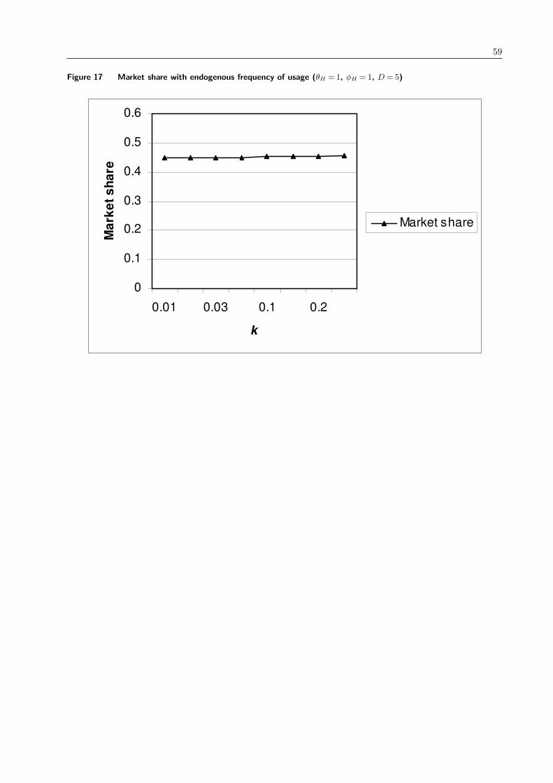
59

Figure 17 Market share with endogenous frequency of usage (θH = 1, φH = 1, D= 5)

0

0.1

0.2

0.3

0.4

0.5

0.6

0.01 0.03 0.1 0.2

k

Ma

rke

t s

ha

re

Market share

60

Figure 18 Payment-per-use with endogenous frequency of usage (θH = 1, φH = 1, D= 5)

0.36

0.38

0.4

0.42

0.44

0.46

0.48

0.01 0.03 0.1 0.2

k

Pa

ym

en

t-p

er-

us

e

Payment-per-

use