Pricing Methods and Hedging Strategiesfor Volatility Derivatives

H. Windcliff∗ P.A. Forsyth†, K.R. Vetzal‡

May 4, 2003

Abstract

In this paper we investigate the behaviour and hedging of discretely observed volatil-ity derivatives. We begin by comparing the effects of variations in the contract design,such as the differences between specifying log returns or actual returns, taking into con-sideration the impact of possible jumps in the underlying asset. We then focus on thedifficulties associated with hedging these products. Naive delta-hedging strategies areineffective for hedging volatility derivatives since they require very frequent rebalancingand have limited ability to protect the writer against possible jumps in the underlyingasset. We investigate the performance of a hedging strategy for volatility swaps thatestablishes small, fixed positions in straddles and out-of-the-money strangles at eachvolatility observation.

1 Introduction

Recently there has been some interest in developing derivative products where theunderlying variable is the realized volatility or variance of a traded financial assetover the life of the contract. The motivation behind introducing volatility derivativeproducts is that they could be used to hedge vega exposure or to hedge against implicitexposure to volatility, such as expenses due to more frequent trades and larger spreadsin a volatile market. In addition, these products could be used to speculate on futurevolatility levels or to trade the spread between the realized and implied volatility levels.

The simplest such contracts are volatility and variance swaps. For example, thepayoff of a volatility swap is given by:

volatility swap payoff = (σR −Kvol)×B , (1)

∗School of Computer Science, University of Waterloo, Waterloo ON, Canada N2L 3G1,hawindcliff@elora.math.uwaterloo.ca†School of Computer Science, University of Waterloo,Waterloo ON, Canada N2L 3G1,

paforsyt@elora.math.uwaterloo.ca‡Centre for Advanced Studies in Finance, University of Waterloo, Waterloo ON, Canada N2L 3G1,

kvetzal@watarts.uwaterloo.ca

1

where σR is the realized annualized volatility of the underlying asset, Kvol is the an-nualized volatility delivery price and B is the notional amount of the swap in dollarsper annualized volatility point. More complex derivative contracts are also possible,such as volatility options and products which cap the sizes of the discretely sampledreturns.

The analysis of variance is inherently easier than the analysis of volatility andconsequently a lot of work in this area [4, 7, 5, 11] has focused on variance products.There are two commonly proposed hedging models for variance. The first involveshedging with a log contract [17], which can be approximated by trading in a largenumber of vanilla instruments [4, 8]. A second hedging approach involves direct delta-hedging of the variance product [11]. Interestingly, the proponents of each methodindicate that the other method is likely to fail in the presence of transaction costs, apoint we will investigate in this paper. Further, most analytic work [4, 8, 12] specifiescontinuously realized variance, whereas in practice the variance is discretely monitored.

Another collection of papers has focused on volatility derivative products, consider-ing them to be a square root derivative of variance as discussed in [8]. In [2] the authorsprovide a volatility convexity correction relating variance and volatility products. Oneproblem with hedging volatility products is that they require a dynamic position inthe log contract, which will result in a large amount of trading in far out-of-the-moneyvanilla instruments. Due to the difficulties with hedging these products, some authorshave even suggested pricing these products via expectation in the real physical measure[13].

In this paper we develop pricing and hedging methods for discretely sampled volatil-ity derivatives. We focus on the structure that is imposed by the design of the contractrather than on a specific model for the stochastic process followed by the underlyingasset. We will find that the contract structure will affect the feasibility of varioushedging methods when applied to these products. Even in a constant volatility Black-Scholes setting, delta hedging strategies must be rebalanced so frequently that they arenot a practical method for hedging discretely observed volatility. Further, if there arepossible jumps in the underlying asset price then even if the delta hedge is rebalancedvery frequently it does not effectively manage downside tail events. As an alternative,we will investigate the performance of a delta-gamma hedging strategy with an ap-propriate selection of vanilla hedging instruments. This strategy can be viewed as anapproximation of the log contract hedge, while avoiding rebalancing a large numberof positions in far out-of-the-money vanilla instruments. Simulation experiments pro-vided in this paper demonstrate that this technique can provide very effective downsiderisk management. We will conclude by investigating the impact of transaction costson the various proposed hedging strategies.

2 Volatility Derivative Products

In the introduction, we discussed a very simple volatility derivative product, the volatil-ity swap. Even restricting ourselves to volatility swaps, there are many possible con-tract variations. For example, there are many possible ways that the volatility deriva-tive contract may define the realized volatility and many ways that the discretelysampled returns can be calculated. In this section we discuss some common volatility

2

and variance derivative contracts.

2.1 Calculation of Returns

If we sample the underlying asset price at the times:

{tobs,i | i = 0, . . . , N} , (2)

then there are two common contractual definitions of the return during the interval[tobs,i−1, tobs,i]. If we define ∆tobs,i = tobs,i− tobs,i−1 then the actual return is defined tobe:

Ractual,i =S(tobs,i)− S(tobs,i−1)

S(tobs,i−1). (3)

We define the log return to be:

Rlog,i = log(

S(tobs,i)S(tobs,i−1)

). (4)

Both of these definitions of the return involve dividing by the previous asset level andthe contract would need to define how the payoff is calculated in the event that theasset price becomes zero.

2.2 Calculation of Volatility

In addition to specifying how the discretely sampled returns are measured, the contractmust also specify how the volatility or variance is calculated. From a discrete sampleof N returns, the annualized realized volatility, σR,stat, can be measured by:

σR,stat =

√√√√√ AN

N − 1

1N

(N∑i=1

R2i

)−

(1N

N∑i=1

Ri

)2 . (5)

The annualization factor, A, converts this expression to an annualized volatility andfor equally spaced discrete observations is given by A = 1/∆tobs. In order to convertunits of volatility into volatility points we would multiply by 100.

Although this is how one would statistically define an estimate for the standarddeviation of returns from a sample, volatility derivatives often define a simpler approx-imation for the volatility. Since many volatility derivative products are sampled atmarket closing each day and the mean daily returns are typically quite small, often thecontract defines the realized volatility, σR,std, to be:

σR,std =

√√√√A

N

N∑i=1

R2i , (6)

the average of the squared returns. Notice that the factor N/(N−1) has been removedfrom the definition of σR,std since it was used to account for the fact that there is aloss of one degree of freedom used to determine the mean return in (5). In this paperwe will refer to (5) as the statistical realized volatility, whereas we will say that (6) isthe standard realized volatility.

3

2.3 Contractual Payoffs

Once the contract has defined how the volatility is to be calculated, the derivativepayoff can be specified. As mentioned above, the payoff of a volatility swap is givenby:

volatility swap payoff = (σR −Kvol)×B . (7)

There are two objectives that are of interest when pricing volatility swaps. Since thereis no cost to enter into a swap, one objective is to determine the fair delivery priceKvol, which makes the no-arbitrage value of the swap initially zero. The volatilitydelivery price can be found by computing the value of a swap with zero delivery priceand multiplying by erT , where r is the risk-free rate and T is the maturity date of thecontract.

A second objective is to determine the fair value of the volatility swap at sometime during the contract’s life given the initially specified delivery price. Because ofthe simplicity of the payoff of the swap contract, it is sufficient to be able to find theno-arbitrage value of a contract which pays σR at maturity.

In some markets severe volatility spikes are occasionally observed. In order toprotect the short volatility position some contracts cap the maximum realized volatility.For example, a capped volatility swap would have a payoff given by:

capped volatility swap payoff = (min(σR, σR,max)−Kvol)×B . (8)

In the variance swap market the maximum realized volatility is typically set to be 2.5times the variance delivery price. The payoffs for variance based derivative productscan be obtained by substituting in σ2

R in place of σR in the above definitions. Althoughwe will not focus on more complex contract structures in this work, some institutionsdo offer products such as corridor swaps [3].

3 A Computational Model for Pricing Volatility

Derivatives

In this section we describe two computational frameworks, one based on a numericalPDE approach and the other based on Monte Carlo simulation methods, that can beused to price volatility and variance based derivative products. In this paper we focuson our ability to hedge a volatility derivative product with value V = V (S, t; . . .).We utilize numerical PDE methods to obtain accurate delta, ∆ = VS , and gamma,Γ = VSS , hedging parameters. We then simulate the performance of various hedgingstrategies by simulating their performance under the real-world (physical) measure andcompare the resulting distributions of profits and losses.

The numerical experiments provided in this paper assume a jump-diffusion model.The sizes of the jumps, J , are drawn from a lognormal distribution with:

log J ∼ N(µJ , γ2J) . (9)

and the underlying asset price, S, which follows the SDE:

dS = (µ− λm)S dt+ σ(S, t)S dW + (J − 1)S dq , (10)

4

where m = E[J − 1] = exp(µJ + 12γ

2J)− 1 and E[ · ] is the expectation operator. Also,

µ is the drift rate of the underlying asset in the physical measure, σ = σ(S, t) is the(state dependent) volatility function, and dW is an increment from a Wiener process.Jumps in the underlying asset price are modelled by the last term with dq being aPoisson process with arrival intensity λ:

dq =

{1 with probability λdt0 with probability 1− λdt .

(11)

The situation where the underlying asset price evolves continuously without jumps canbe modelled by setting the arrival intensity λ = 0. For simplicity, we assume that nodividends are paid by the underlying asset although it is straightforward to incorpo-rate either a continuous dividend yield or discrete dollar dividends in our numericalframework. We also point out that in our numerical approach it is possible to use anyjump size distribution in place of (9).

3.1 Risk-Neutral Valuation

Some of the numerical results provided in this paper were obtained using Monte Carlosimulation. Further, we will use the risk-neutral valuation ideas presented here toanalyze the asymptotic behaviour of volatility derivative contracts.

Under the risk-neutral measure, Q, the underlying asset follows the SDE:

dS = (r − λm)S dt+ σ(S, t)S dW + (J − 1)S dq . (12)

The local volatility surface, σ(S, t), and the jump parameters λ, µJ and γJ , havebeen selected so that the model correctly prices existing options in the market. Theno-arbitrage value is found by approximating the expectation:

V (S(0), 0) = e−rTEQ[V (S, T ; σR)] , (13)

by averaging over many sample asset paths and computing the realized quantity σRalong each of these paths. Although this technique is very straightforward to imple-ment, it is difficult to obtain accurate estimates of the delta and gamma derivativesthroughout the life of the contract, which are necessary when we simulate the per-formance of various hedging strategies. When a general volatility surface is used wecannot integrate (12) analytically, although we can generate the risk-neutral randomwalks numerically using, for example, an Euler timestepping method.

3.2 Numerical PDE Framework

Many of the results provided in this paper were obtained using a numerical partialdifferential equation (PDE) framework. This allows us to efficiently compute the deltaand gamma derivatives used later in this paper to simulate the performance of varioushedging strategies for these contracts.

In [16] the authors provide an efficient computational model for pricing discretelysampled variance swaps in a Black-Scholes setting. The efficiency of their method comesfrom exploiting the linear structure of variance products and cannot be extended tovolatility derivative products, which have matters complicated by the coupling of therealized returns through the square root function.

5

3.2.1 State Variables and Updating Rules

In order to price a general volatility derivative product we introduce two additionalstate variables. Let P represent the stock price at the previous volatility observationtime and let Z be the average of the squared returns observed to date:

Zi =1i

i∑j=1

R2j . (14)

In some situations it is possible to use a similarity reduction in the variable ξ = S/P .However, for a general volatility function, σ(S, t), this dimensionality reduction is notpossible.

Initially the state variables are set to:

P (0) = S(0) (15)Z(0) = 0 . (16)

These variables are changed only at the discrete volatility sampling times, tobs,i, i =1, . . . , N according to the following jump conditions. If t−obs,i and t+obs,i represent theinstants immediately before and after the ith observation date then:

P (t+obs,i) = S(t−obs,i) , (17)

Z(t+obs,i) = Z(t−obs,i) +R2i − Z(t−obs,i)

i. (18)

The return, Ri, can be computed from the state variables contained in the computa-tional model. For example, if the contract specifies that log returns are used then:

Ri = log

(S(t−obs,i)

P (t−obs,i)

). (19)

The updating rules for the state variables are implicitly defined by the volatilityderivative contract and are independent of any assumptions regarding the behaviourof the underlying asset. We will find that this structure has important ramificationswhen we consider the hedging of these products.

3.2.2 Evolution Equations Between Volatility Observations

Between the discrete volatility sampling times the state variables do not change. Con-sequently, between observations we can think of the value of the volatility derivativeproduct as being a function of the underlying asset price S and time t, parameterizedby the state variables:

V = V (S, t; P,Z) . (20)

So far in this section our discussion has been independent of any assumptions regardingthe behaviour of the underlying asset. In order to model the behaviour of the contractbetween volatility observations we need to make some assumptions. In this paper wewill work with a one factor model that utilizes a local volatility surface. In someexamples we allow the possibility of jumps in the underlying asset price. It could

6

be argued that it would also be useful to consider a stochastic volatility model as in[12, 13, 11]. However, our focus in this paper is to investigate hedging results thatare independent of the assumptions about the evolution of the underlying asset. Thesimple one factor, jump-diffusion model is sufficient to illustrate our point that deltahedging strategies are ineffective for managing the risk associated with these products.

In the jump-diffusion model, the value of the volatility derivative satisfies the partialintegro-differential equation (PIDE):

Vt + (r − λm)SVS +12σ2(S, t)S2VSS − rV + λE[∆V ] = 0 , (21)

where:

E[∆V ] = E[V (JS, t)]− V (S, t) (22)

=∫V (JS, t)p(J)dJ − V (S, t) , (23)

and p( · ) is the probability density function for the jump size. This equation is solvedbackwards from maturity, t = T , to the present time, t = 0, to determine the currentfair value for the contract. For a description of the computational methods used tosolve this PIDE the reader is referred to [9].

3.2.3 Maturity Conditions

If the volatility is defined without the mean according to (6) then it is straightforwardto specify the value of the volatility derivative as a function of the state variables. Forexample, from the contractual payoff we see that the appropriate terminal conditionfor a volatility swap would be:

V (S, T ; P,Z)volatility swap = (100√AZ −Kvol)×B , (24)

where Kvol is the volatility delivery price, A is the annualization factor and B is thenotional amount. The terminal condition for a variance swap would be:

V (S, T ; P,Z)variance swap = (100AZ −Kvar)×B , (25)

where Kvar is the variance delivery price. More exotic volatility payoffs are also possiblein this framework. For example the terminal condition for a capped volatility swapwould be:

V (S, T ; P,Z)capped volatility swap = (min(100√AZ, σR,max)−Kvol)×B . (26)

In summary, the value of the volatility derivative product is a time-dependent func-tion of three space-like variables. After applying the terminal condition at maturity wesolve a collection of independent backward equations (21) between the discrete obser-vation times. At the discrete volatility sampling times we apply the jump conditions(17)-(18). When we reach the date of sale of the contract, the no-arbitrage value ofthe volatility derivative is given by:

V (S = S(0), t = 0; P = S(0), Z = 0) . (27)

An example of this technique applied to a different type of path-dependent option isgiven in [23].

7

3.2.4 Asymptotic Boundary Conditions

In order to complete the numerical problem, we determine appropriate conditions atthe boundary of the computational domain, S = Smin and S = Smax. Although it ispossible to reduce the boundary truncation error in the region of interest near S = S(0),t = 0, to an arbitrary tolerance by sufficiently extending the computational domain[14], it is of practical interest to accurately specify the boundary behaviour in order toreduce the number of nodes in the grid.

The payoff of a volatility option or swap (capped or otherwise) is linear in σR.Thus, it suffices to analyze the asymptotic behaviour of a contract that pays off therealized volatility at maturity, V (S, T ) = σR. To determine appropriate boundaryconditions we look at the asymptotic form of the jump conditions. Notice that thesecan be thought of as specifying initial data over a given volatility observation period.

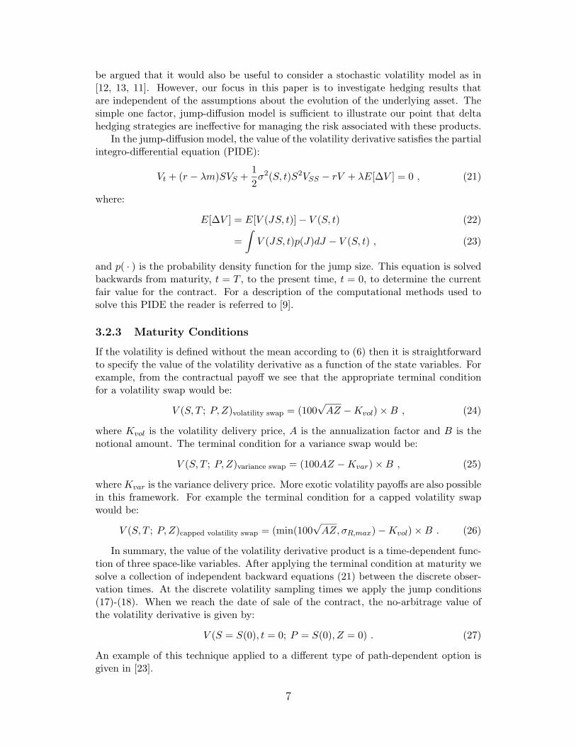
We begin by analyzing the value of the volatility derivative at the instant imme-diately preceding the jth volatility observation, t−obs,j . If we let F(t) represent theinformation available at time t then, assuming that σR is defined according to (6),using risk-neutral valuation we find:

V (S, t−obs,j) = e−r(T−tobs,j)EQ[σR|F(t−obs,j)] (28)

= e−r(T−tobs,j)√A

NEQ

√√√√j−1∑

i=1

R2i +R2

j +N∑

i=j+1

R2i

∣∣∣∣F(t−obs,j)

. (29)

The first term in the square root is a constant, independent of S, as it represents thepast volatility observations. The second term, R2

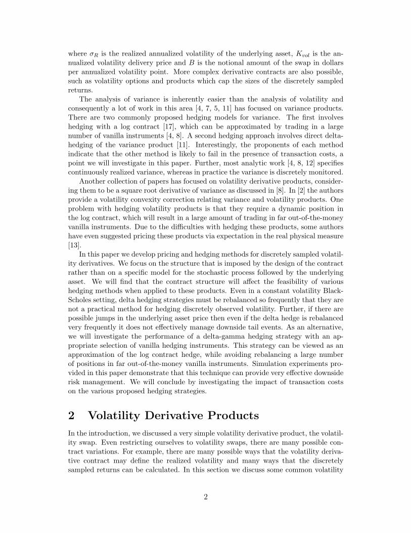
j , represents the current volatilityobservation. It depends on S in a the way specified by the contractual definition of theobserved returns. At time t−obs,j the last term is random, corresponding to the level offuture volatility samples. This decomposition is illustrated in Figure 1.

Suppressing the explicit reference to the time, t−obs,j , for S far away from the pre-vious asset level P , if the volatility function is suitably well behaved, the currentvolatility observation, R2

j , will dominate in (29). Thus the value is approximately alinear function of the current return at the boundaries. For actual returns we have:

Rj =S − PP

,dRjdS

= 1/P,d2RjdS2

= 0 . (30)

This indicates that VSS → 0 at both boundaries when actual returns are specified. Forlog returns we have:

Rj = log(S/P ),dRjdS

= 1/S,d2RjdS2

= −1/S2 , (31)

which indicates that VSS → 0 as the asset level becomes large. In practice, the volatilityderivative contract would need to specify how future returns would be computed in theevent that the asset price became zero. However, the lower boundary is an outflowboundary [22] and using the approximation VSS = 0 at S = S1 will not affect thesolution near S = S(0), t = 0, assuming that the computational domain is sufficientlywide [14].

8

Asset Price

Rea

lized

Vol

atili

tyFuture volatility

Past volatility

Currentvolatility

S=P

Figure 1: Heuristic decomposition of the realized volatility in terms of the past, currentand future volatility samples, at a time immediately preceeding a volatility observation.

4 Pricing Volatility Exposure

Now that we have described numerical methods for pricing these contracts we can in-vestigate the impact of various modelling assumptions and contractual designs on thefair value of these products. Specifically, we would like to determine how robust thepricing and hedging results are against changes in our assumptions regarding the mod-elling of the underlying asset price movements. Also, we would like to understand theeffect that variations in the contract design will have on the pricing of these products.

4.1 Effect of the Underlying Asset Price Model

In this section we compare the value of the volatility swap assuming a jump-diffusionmodel, a local volatility function model with no jumps, and a constant volatility modelwith no jumps. We consider a market where the underlying asset price contains possiblejumps and that these jumps are priced into a market of available options. The optionsmarket consists of European call and put options with strikes spaced by ∆K = $10 andmaturities spaced by ∆T = .1 year, or approximately one month. We assume that thewriters of options in this market use the risk-adjusted parameters λ = .1, µJ = −.9,γJ = .45 and σ = .2 to price these instruments and charge the fair value.1 Thisdefines a market consistent with the jump-diffusion model parameters given above. Inorder to facilitate comparisons between the various models of the underlying asset,we calibrated a local volatility function2 as described in [6], and a constant implied

1These parameters are approximately the values reported in [1], which the authors found were implied ina certain set of S&P options market prices.

2Source: the local volatility function was computed using the Calcvol volatility surface calibration pro-gram developed at Cornell University.

9

0

0.2

0.4

0.6

0.8

Loca

lVo

latil

ity

0

0.2

0.4

0.6

Time to Maturity 80

100

120

Asset Level

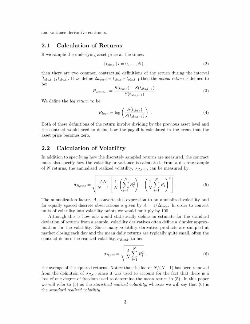
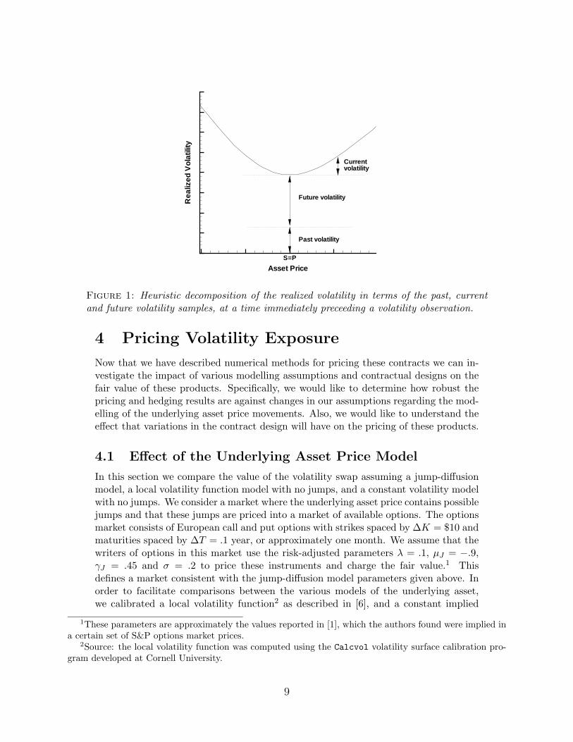
Figure 2: Local volatility function computed to match the prices of call and put options ina synthetically generated market. The options were priced assuming r = .05, σ = .2 withjump parameters λ = .1, µJ = −.9 and γJ = .45, S(0) = $100.

volatility to these market prices of vanilla options.Although jump-diffusion models have recently been gaining popularity, solving the

PIDE (21) for exotic options requires advanced numerical software and is somewhatmore complex than the techniques required to value exotic options in the standardBlack-Scholes framework without jumps. As a result it is common to use local volatil-ity surfaces in order to price exotics consistently with observed market prices. If wecalibrate a local volatility function consistent with the option prices observed in oursynthetic market, the resulting local volatility function is as shown in Figure 2. Thelocal volatility function exhibits the skewed smile that is often observed in optionsmarkets, which flattens off for longer maturities.

Even simpler than using a local volatility function, we can consider matching asingle constant implied volatility, σimp, using an at-the-money option with the samematurity as the volatility swap we are pricing. We find that an implied volatility ofσimp = 0.25046 matches the price of an at-the-money option in our synthetic market.

We now have three possible models for the underlying asset price that are all plausi-ble given currently observed market prices. In practice, the person hedging the volatil-ity derivative would not know which of these (or other) models truly generates theunderlying price process and would need to choose among them. Here we briefly dis-cuss some of the similarities and differences that can occur in the valuation and hedgingof volatility products under these different models.

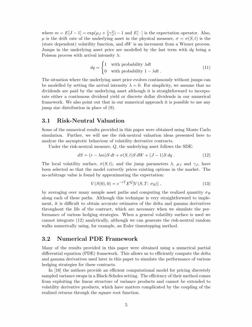
In Figure 3(a) we see that there are some qualitative properties that hold for allof the models for the underlying asset process. All models have a minimum occurringnear the initial asset level (corresponding to the previous asset price during the first

10

Asset Price

Val

ue

50 100 150 2000

10

20

30

40

50

60

70

80

90

100

Jump DiffusionConstant Vol.Local Vol. Function

(a) The effect of assumptions regardingthe underlying asset price process. Thelocal volatility function and constant im-plied volatilities were chosen to be consis-tent with the pricing of vanilla call and putoptions under the jump-diffusion process,which utilized σ = .20, µJ = −.9, γJ = .45and λ = .1.

Asset Price

Val

ue

40 60 80 100 120 140 160 180 2000

10

20

30

40

50

60

70

80

90

100

Actual ReturnsLog ReturnsCapped Contract

(b) The effect of the contractually definedreturn on the fair value of a volatility swapcontract. The capped contract used log re-turns with a maximum realized volatility ofσR,max = .50. The underlying asset pricefollowed geometric Brownian motion withσ = .20, S(0) = $100, and no jumps.

Figure 3: The volatility swap payoff was calculated using standard realized volatility,T = .5, Kvol = 0 and B = 1 with daily observations, ∆tobs = .004. The initial asset pricewas S(0) = $100 and the risk-free rate was r = .05.

volatility sample). As one moves away from the previous asset level, the value of thevolatility swap increases because more volatility will accrue during the current volatilitysample. Looking at the slope, which corresponds to the delta hedging parameter, wesee that a delta hedging strategy will hold a long position in the underlying asset ifS > P to protect against further increases in the asset price. Similarly, a delta hedgingstrategy will hold a short position in the underlying asset if S < P to protect againstthe volatility accrued if the asset value decreases further.

As we would expect, there are some quantitative differences between the valuationsobtained using the different models for the underlying asset. Although the constantvolatility model and the jump-diffusion model give very similar solutions, the localvolatility function model gives somewhat different results. This is because the localvolatility function behaves as if the volatility is state dependent, and from Figure 2 wesee that the local volatility function imposes a higher volatility when the asset priceis either well below or well above S(0) = $100. Although the valuations, and hencethe implied hedging positions, differ slightly for the various underlying asset models,the qualitative properties, and the general hedging results given in Section 5 based onthese qualitative properties, continue hold for different models of the underlying asset.

4.2 The Influence of Product Design on Pricing

In this section, we investigate the impact of variation in the design of the contract onthe fair volatility delivery price. Specifically, we investigate the differences caused by

11

Jumps Sampling frequency Return type Kvol

(volatility points)

No Daily Log 19.961Actual 19.961Capped 19.961

No Weekly Log 19.806Actual 19.835Capped 19.806

Yes Daily Log 25.440Actual 23.052Capped 21.354

No Daily Log (σR,stat) 19.961Weekly Log (σR,stat) 19.794

Table 1: The impact of variations in the contract definition on the fair forward deliveryprice. The capped contracts specified a maximum realized volatility of σR,max = .50 withlog returns. Unless mentioned otherwise, the volatility swap specified standard calculationof realized volatility, T = .5, and B = 1. For daily observations ∆tobs = .004 while forweekly observations ∆tobs = .02. The risk-free rate is r = .05 and a constant volatilityof σ = .20 was used. The experiments that included jumps in the underlying asset pricespecified λ = .1, µJ = −.9 and γJ = .45.

the definition of return, the frequency of observation and the impact of whether or notthe mean is included in the calculation of volatility. The numerical computations givenin this section were performed using a sufficiently fine discretization that the solutionsare accurate to within approximately ±.001.

In Table 1 we see that when the volatility is sampled very frequently (i.e. dailyor weekly) and the asset price evolves continuously, the definition of the return hasvery little impact on the fair value of the contract. The capped contract used logreturns and the total realized volatility was limited to a maximum of σR,max = .50.In the simulations that were carried out, with daily and weekly sampling the cap wassufficiently large that it never affected the payoff when there were no jumps in theunderlying asset price. Figure 3(b) illustrates the differences between the realizedvolatility when the contract specifies log returns, actual returns and a cap on the fairvalue of these contracts. The sampling frequency has a larger impact on the fair valueof these contracts, with differences between weekly and daily sampling occurring in thethird digit. As a result, hedging strategies based on a continuously observed volatilitymay become less effective for longer sampling intervals.

If the underlying asset price jumps then the differences between log, actual andcapped returns become more noticeable. In Table 1 we see that the capped contractis less affected when we introduce a jump component to our simulation model. In thiscase we have introduced jumps according to a Poisson process with intensity, λ = .1.If a jump occurs, the size of the jump is drawn from a lognormal distribution withmean, µJ = −.9, and standard deviation, γJ = .45. Notice in Figure 3(b) that thevalue of the contract using log returns increases more quickly than the value of thecontract using actual returns when S � P . Since on average the jumps are downward,

12

contracts defined using log returns are the most dramatically impacted by the jumpcomponent.

At the bottom of Table 1 we investigate the impact of statistically defining therealized volatility as in equation (5) compared with the more common standard defi-nition of the realized volatility given by equation (6). We find that for daily samplingthe differences are minimal, affecting the fifth digit. As the sampling becomes lessfrequent, there is more difference between the fair values of the contracts depending onwhether or not the mean is included in the calculation of the volatility. For examplewith weekly sampling, the effects of whether or not the mean in included lie in thefourth digit.

5 Hedging Volatility Exposure

We will see that hedging volatility swap contracts is more difficult than hedging simplevanilla call and put options. There are two standard dynamic approaches that wecan use to hedge these contracts; delta hedging and delta-gamma hedging. In thissection we look at the relative merits of each of these approaches and investigate theperformance of these hedging methods considering the effects of transaction costs andjumps in the underlying asset price.

In this paper we computed the delta and gamma hedging parameters using a suf-ficiently fine mesh during the numerical PDE computations such that further refine-ments did not appreciably affect the hedging results provided in this section. We thenperformed simulations where the asset path evolved according to (10) using non-risk-adjusted parameters (i.e. in the physical measure) in order to investigate the perfor-mances of the various hedging strategies. The profit and loss (P&L) is the value of thehedging portfolio less the value of the payout obligation for the short volatility swapat the maturity of the contract. For each simulation study we provide the expectedprofit (or loss if negative), the standard deviation of the P&L distribution and the 95%conditional value at risk (CVaR) which is the average of the worst 5% of the outcomesin the P&L distribution. The CVaR measure satisfies certain axiomatic properties[18] that are consistent with the notion of risk. It has also been recognized as a morerobust measure downside risk than standard value at risk (VaR) when the profit andloss distribution has fat tails [18].

5.1 Model-Independent Hedging Results

There are two main model-independent results that we focus on in this section. Theseare imposed on us by the structure of the volatility contract and consequently hold forgeneral models of the price movements by the underlying asset. First, we demonstratethat discretely observed volatility derivative products require very frequent rebalancing.Second, we offer suggestions as to appropriate hedging instruments based on the profileof the realized volatility during the current observation.

5.1.1 Frequency of Rebalancing

Consider the situation of the investor who is short the floating leg of the volatility swap.In theory, one can delta hedge risk exposure to a short position in a derivative contract

13

Profit and Loss DistributionHedge type ∆thedge Mean Std. dev. 95% CVaR

No hedge None -.005 1.27 -2.66Delta hedge ∆tobs -.002 1.26 -2.65

∆tobs/2 -.003 .89 -1.86∆tobs/4 -.002 .63 -1.32

Delta-Gamma hedge ∆tobs .004 .03 -.05

Table 2: Statistics of the profit and loss distribution of a discretely hedged, short volatilityswap position. The volatility swap specified log returns, no mean, T = .5, Kvol = 19.961,∆tobs = .004, and B = 1. It was assumed that r = .05, µ = .1 and σ = .2. The numericalcomputations were obtained from Monte Carlo experiments using 1,000,000 simulations.

with value V (S, t) by holding VS(S, t) shares in the underlying asset at all times. Thisstrategy can be viewed as setting up a local tangent line approximation to the valueof the volatility swap. In practice, we define a regular hedging interval, ∆thedge, andadjust the hedging position at th = h∆thedge, h = 1, 2, . . . , nh, where nh = bT/∆thedgec.In order to delta hedge over the time interval [th, th+1), the investor holds VS(S(th), th)shares of the underlying asset. In order for the discrete delta hedging strategy to beaccurate we need to choose ∆thedge sufficiently small so that:

VS(S(th), th;P (th), Z(th)) ≈ VS(S(t), t;P (t), Z(t)) (32)

for all t ∈ [th, th+1), where we have explicitly written the dependence of the underlyingasset price and state variables on time. Since the state variables change at the volatilitysampling times, we require that the delta hedging interval cannot be longer than thevolatility sampling period, ∆thedge ≤ ∆tobs.

To illustrate the fact that very frequent rebalancing is required for discretely ob-served volatility derivative contracts, we consider a very simple Black-Scholes settingwith a constant volatility model. Focusing on the middle section of Table 2 we see thatthe delta hedging strategy must be rebalanced four times per observation in order tosubstantially reduce the risk when compared with the unhedged position. This exces-sive rebalancing makes delta hedging appear to be inappropriate for these contracts.In a more realistic non-constant volatility model we would need to delta hedge thecurrent volatility exposure as well as manage changes in the level of volatility, makingthis hedging approach even less viable. In the next section we will consider a moreflexible delta-gamma hedging strategy. We will find that this hedging strategy can pro-vide good performance even if we only rebalance our hedging positions at the volatilityobservation times.

5.1.2 Appropriate Hedging Instruments

We have seen that delta hedging strategies must be rebalanced much more frequentlythan the volatility sampling frequency. We now investigate the structure of the up-dating rules for the state variables in order to gain insight as to why the underlyingasset is not an appropriate hedging instrument. One reason for this is illustrated inFigure 4. In this figure we see that when S = P the tangent to the curve denoting the

14

Asset Price

Val

ue

Delta Hedge

Delta-GammaHedge

Volatility Swap(Target)

S=P

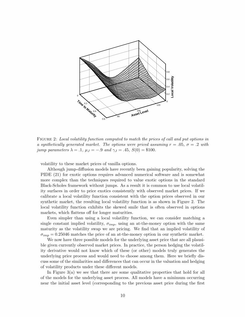
Figure 4: Demonstration of the ability of a delta-gamma hedging strategy to match thevalue profile of a daily sampled volatility swap. The delta-gamma hedge was constructed us-ing an at-the-money straddle position as the secondary hedging instrument. The delta hedgetakes no position in the underlying asset and is unable to hedge against price movementsin either direction.

value as a function of underlying asset price is horizontal. This indicates that VS ≈ 0and that the delta hedge does not take a position in the underlying asset at this time.Unfortunately, most of the time S ≈ P since the previous asset level is set to thecurrent asset level at each volatility observation date. This is evident in Table 2 wherewe see that delta hedging only at the volatility sampling times yields almost identicalresults to the situation where the writer elects not to hedge the volatility product at all.The underlying asset is not flexible enough to simultaneously hedge the volatility thatwould be accrued if the asset price moved in either direction. As a result, in order todelta hedge our volatility exposure we will need to adjust our hedging positions muchmore frequently than the volatility sampling frequency.

Looking at Figure 4, we see that the value of the volatility swap attributed tothe current sample is quite similar to the payoff of a straddle position struck at theprevious asset level. If the underlying asset price moves away from the previous assetlevel in either direction, then this sample will accrue a positive amount towards thefinal realized volatility. As a result, we suggest constructing straddle or out-of-the-money strangle positions at each volatility observation. Although this will still involverebalancing at each volatility observation, the positions taken will be quite small sincewe are only hedging the volatility that accrues over the current volatility samplingperiod.

In order to hedge a short position in the volatility derivative with price given byV , a delta-gamma hedging strategy holds positions x1 in the underlying asset and x2

15

in appropriate short-term options according to:

x1 = VS − x2IS , (33)

x2 =VSSISS

, (34)

where IS , ISS are the delta and gamma respectively of the secondary instruments. Wewill choose the secondary instruments so that ISS is large enough so that the positionin the secondary instruments given by (34) does not become too large. Although theweights of the hedging instruments have been chosen to locally match the delta andgamma of the product we are hedging, we have also chosen the secondary instrumentsto be consistent with the far-field behaviour. As a result, if there are large asset priceswings, the proposed hedging strategy qualitatively matches the target profile. InSection 5.4 we will see that this strategy is closely related to a hedging strategy forvariance swaps that utilizes a log contract.

We assume that the writers set up their hedging positions using short term, ex-change traded options. Exchange traded options tend to have a fixed range of avail-able strike prices. In our experiments, it was assumed that the strike prices of availableoptions used as secondary instruments were spaced by ∆K = $10 and the initial assetprice was S(0) = $100. The delta-gamma hedging strategy constructs either straddleor out-of-the-money strangle positions at each volatility observation using the strikeprices nearest the current asset price while attempting to maintain a roughly symmet-ric risk exposure to large price movements. Specifically, if Ki ≤ S ≤ Ki+1 at timetobs,j , then we construct:

• A straddle position with strike Ki if S −Ki < .2∆K.

• A straddle position with strike Ki+1 if Ki+1 − S < .2∆K.

• An out-of-the-money strangle position using put options with strike Ki and calloptions with strike Ki+1 otherwise.

In order to avoid excessive transaction costs, once we establish an out-of-the-moneystrangle position, we will only change the secondary hedging instruments if the assetlevel moves beyond the strike prices of either the call or put option.

In our experiments we assume that the options in the market mature at approx-imately monthly intervals where ∆T = .1 year. In general we use the shortest termoptions whose maturity date is later than the next volatility observation since shortterm options have a higher ratio of gamma to value, which will be useful in reducingtransaction costs. However, as we near the maturity date of the secondary optionstheir gammas become too localized around the strike prices and we choose to restrictourselves to using options with a minimum remaining time to maturity of half of amonth, i.e. T − t ≥ .05 years.

In Table 2 we see that the delta-gamma hedging strategy performs very well relativeto the delta hedging strategy. If we only adjust the delta-gamma hedge at the volatilityobservations, the standard deviation of the profit and loss distribution is reduced by afactor of over 20 when compared with a delta hedging strategy that is re-balanced fourtimes per volatility sampling period. We refer to this delta-gamma hedging strategyas a semi-static hedge because it constructs small, fixed positions at each volatilityobservation which are not adjusted until the next volatility sampling date.

16

Profit and Loss DistributionHedge type ∆thedge Mean Std. dev. 95% CVaR

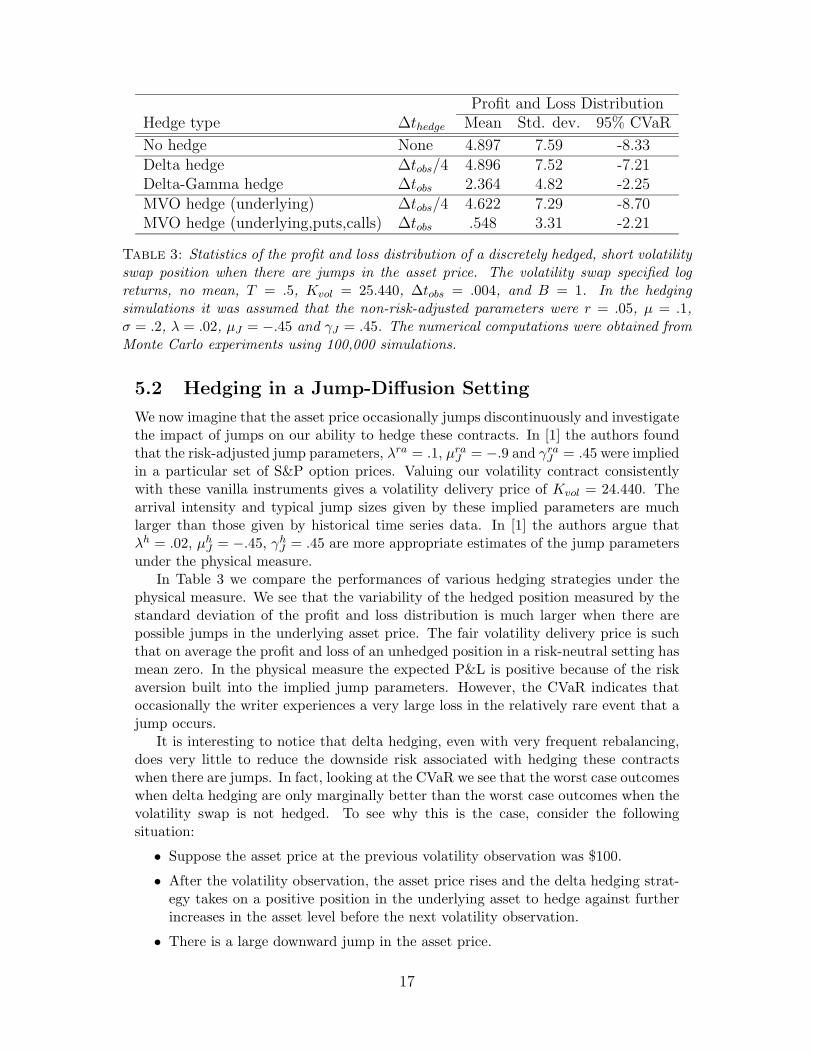
No hedge None 4.897 7.59 -8.33Delta hedge ∆tobs/4 4.896 7.52 -7.21Delta-Gamma hedge ∆tobs 2.364 4.82 -2.25MVO hedge (underlying) ∆tobs/4 4.622 7.29 -8.70MVO hedge (underlying,puts,calls) ∆tobs .548 3.31 -2.21

Table 3: Statistics of the profit and loss distribution of a discretely hedged, short volatilityswap position when there are jumps in the asset price. The volatility swap specified logreturns, no mean, T = .5, Kvol = 25.440, ∆tobs = .004, and B = 1. In the hedgingsimulations it was assumed that the non-risk-adjusted parameters were r = .05, µ = .1,σ = .2, λ = .02, µJ = −.45 and γJ = .45. The numerical computations were obtained fromMonte Carlo experiments using 100,000 simulations.

5.2 Hedging in a Jump-Diffusion Setting

We now imagine that the asset price occasionally jumps discontinuously and investigatethe impact of jumps on our ability to hedge these contracts. In [1] the authors foundthat the risk-adjusted jump parameters, λra = .1, µraJ = −.9 and γraJ = .45 were impliedin a particular set of S&P option prices. Valuing our volatility contract consistentlywith these vanilla instruments gives a volatility delivery price of Kvol = 24.440. Thearrival intensity and typical jump sizes given by these implied parameters are muchlarger than those given by historical time series data. In [1] the authors argue thatλh = .02, µhJ = −.45, γhJ = .45 are more appropriate estimates of the jump parametersunder the physical measure.

In Table 3 we compare the performances of various hedging strategies under thephysical measure. We see that the variability of the hedged position measured by thestandard deviation of the profit and loss distribution is much larger when there arepossible jumps in the underlying asset price. The fair volatility delivery price is suchthat on average the profit and loss of an unhedged position in a risk-neutral setting hasmean zero. In the physical measure the expected P&L is positive because of the riskaversion built into the implied jump parameters. However, the CVaR indicates thatoccasionally the writer experiences a very large loss in the relatively rare event that ajump occurs.

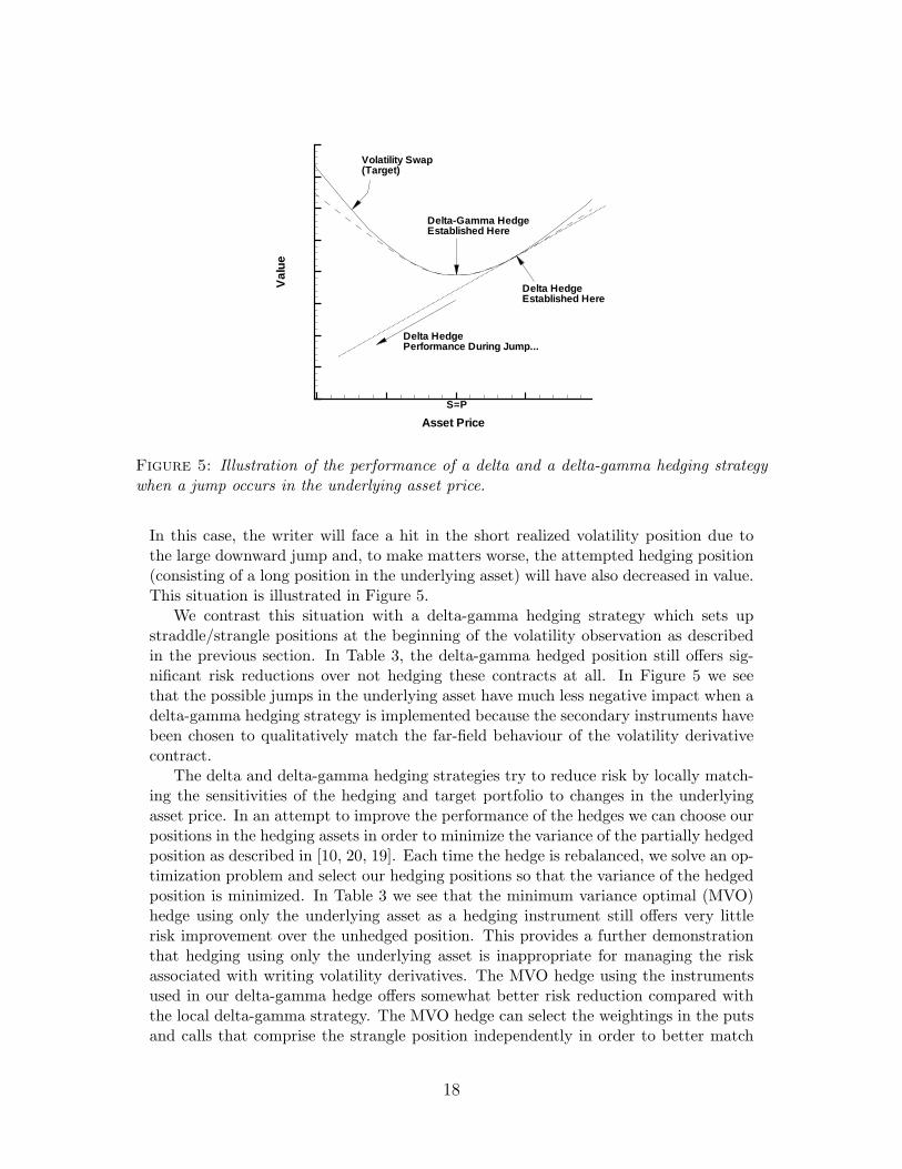
It is interesting to notice that delta hedging, even with very frequent rebalancing,does very little to reduce the downside risk associated with hedging these contractswhen there are jumps. In fact, looking at the CVaR we see that the worst case outcomeswhen delta hedging are only marginally better than the worst case outcomes when thevolatility swap is not hedged. To see why this is the case, consider the followingsituation:

• Suppose the asset price at the previous volatility observation was $100.

• After the volatility observation, the asset price rises and the delta hedging strat-egy takes on a positive position in the underlying asset to hedge against furtherincreases in the asset level before the next volatility observation.

• There is a large downward jump in the asset price.

17

Asset Price

Val

ue

Delta-Gamma HedgeEstablished Here

Volatility Swap(Target)

Delta HedgeEstablished Here

Delta HedgePerformance During Jump...

S=P

Figure 5: Illustration of the performance of a delta and a delta-gamma hedging strategywhen a jump occurs in the underlying asset price.

In this case, the writer will face a hit in the short realized volatility position due tothe large downward jump and, to make matters worse, the attempted hedging position(consisting of a long position in the underlying asset) will have also decreased in value.This situation is illustrated in Figure 5.

We contrast this situation with a delta-gamma hedging strategy which sets upstraddle/strangle positions at the beginning of the volatility observation as describedin the previous section. In Table 3, the delta-gamma hedged position still offers sig-nificant risk reductions over not hedging these contracts at all. In Figure 5 we seethat the possible jumps in the underlying asset have much less negative impact when adelta-gamma hedging strategy is implemented because the secondary instruments havebeen chosen to qualitatively match the far-field behaviour of the volatility derivativecontract.

The delta and delta-gamma hedging strategies try to reduce risk by locally match-ing the sensitivities of the hedging and target portfolio to changes in the underlyingasset price. In an attempt to improve the performance of the hedges we can choose ourpositions in the hedging assets in order to minimize the variance of the partially hedgedposition as described in [10, 20, 19]. Each time the hedge is rebalanced, we solve an op-timization problem and select our hedging positions so that the variance of the hedgedposition is minimized. In Table 3 we see that the minimum variance optimal (MVO)hedge using only the underlying asset as a hedging instrument still offers very littlerisk improvement over the unhedged position. This provides a further demonstrationthat hedging using only the underlying asset is inappropriate for managing the riskassociated with writing volatility derivatives. The MVO hedge using the instrumentsused in our delta-gamma hedge offers somewhat better risk reduction compared withthe local delta-gamma strategy. The MVO hedge can select the weightings in the putsand calls that comprise the strangle position independently in order to better match

18

the target profile of the contract that we are hedging.

5.3 Hedging with a Bid-Ask Spread

We now investigate the impact of transaction costs on the valuation and hedging ofthese contracts. Specifically, we assume that the hedger incurs transaction costs dueto a bid-ask spread. We define the one-way transaction cost loss due to trading in theunderlying asset to be:

κ =(

12

)Sask − Sbid

Sask. (35)

Typically, the bid-ask spread for liquidly traded assets is quite small and in our exper-iments we use κ = .001 or 10 basis points. On the other hand, the bid-ask spread forexchange traded options can be quite large, and typical values for the transaction costparameter for the secondary instruments would be around κSI = .05.3

When there are transaction costs [21] we replace (21) with:

Vt + rSVS +12σ2S2VSS − κσS2

(√2

π∆thedge

)|VSS | − rV = 0 . (36)

The new term containing |VSS | estimates the expected costs of changing the deltahedged position at the end of the hedging interval. In general this equation is non-linear and must be solved numerically. However, when actual returns are specified thegamma, VSS , is always positive and we can simply use the Leland volatility correction[15]:

σLeland = σ

(1 +

(√8

π∆thedge

)κ

σ

)1/2

. (37)

Even when log returns were specified, the regions where the gamma changes sign areso far away from the region of interest (see Figure 3(b)) that we could not noticeany differences between the solution computed using (36) compared with the solutioncomputed using (21) with (37).

Assuming that κ = .001 and re-balancing the delta hedged position four timesper volatility observation, ∆thedge = .001, the cost of hedging the realized volatilityis $21.786 at time t = 0, giving a fair delivery price at maturity of Kvol = 22.338.Comparing with the fair delivery price without considering transaction costs givenin Table 1, we see that the expected transaction costs are $2.377. In other words,approximately 10% of the value of the delivery price is lost through hedging transactioncosts. If we do choose not to hedge the product, then at maturity we expect to haveapproximately $2.377 in profit, at the expense of the additional risk we take on by nothedging. This is very close to the expected excess of the unhedged position in Table 4.

3An alternative to exogenously specifying the option bid-ask spread would be to determine the inferredspread in terms of the bid-ask spread for the underlying asset using a transaction cost model. However,the rebalancing interval used to hedge the vanilla instruments would probably be much longer than therebalancing interval used to hedge the volatility derivative contract, making the implied bid-ask spreadsomewhat arbitrary. Instead, we choose κSI to be representative a typical options market.

19

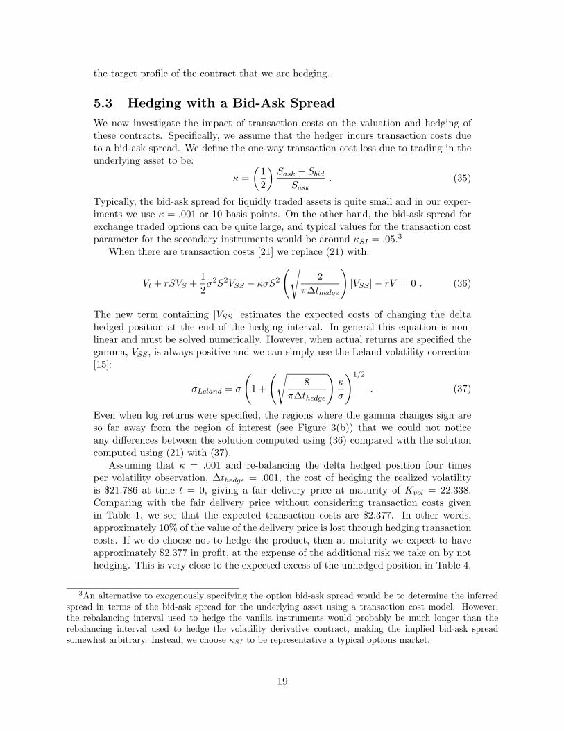
Profit and Loss DistributionHedge type ∆K κSI Mean Std. dev. 95% CVaR

No hedge N/A N/A 2.375 1.26 -.27Delta hedge N/A N/A -.427 .68 -1.84Delta-Gamma hedge $10 .05 -3.564 .85 -5.35

$10 .001 .843 .15 .50$20 .001 .991 .23 .55

Table 4: Statistics of the profit and loss distribution of a discretely hedged, short volatilityswap position when there are transaction costs. The volatility swap specified log returns,no mean, T = .5, Kvol = 22.338, ∆tobs = .004, and B = 1. It was assumed that r = .05,µ = .1, σ = .2, κ = .001 and S(0) = $100. The numerical computations were obtainedfrom Monte Carlo experiments using 1,000,000 simulations.

If we attempt to delta hedge the contract we find that the profit and loss distri-bution has a negative mean value, indicating that equation (36) has underestimatedthe expected transaction costs. To explain this, recall that the Leland transaction costmodel uses a gamma approximation in order to determine the expected change in theposition of the hedging asset. In Figure 4 we see that this second-order approximationunderestimates the curvature, and hence the expected transaction costs, for larger as-set price movements. The risk associated with the delta hedged position is similar tothat found in Table 2 in the absence of a bid-ask spread.

To this point, the delta-gamma hedging strategy that involves setting up straddle-strangle positions at each volatility observation has performed very well. However, thebid-ask spread on exchange traded options is quite large and typical values might bearound κSI = .05. We see in the bottom row of Table 4 that when faced with theselarge transaction costs, the delta-gamma hedging strategy is no longer feasible.

On the other hand, it might be plausible to assume that the institution hedgingthe volatility swap has clients who can act as natural counterparties to the positionsin these vanilla options. In this situation we assume a much smaller transaction costassociated with trading in the secondary instruments, κSI = .001. Now the delta-gamma hedging strategy incurs fewer transaction costs and has less variability thanthe delta hedged position with transaction costs. In fact, now approximately half ofthe additional mark-up due to the transaction costs is now retained as profit and thedelta-gamma hedging is so effective that even the 95% CVaR is positive.

When there are transaction costs there are tradeoffs that must be considered in theselection of the hedging instruments. At the bottom of Table 4 we compare the per-formance of the delta-gamma hedging strategy when ∆K = $10 and when ∆K = $20.We see that by choosing wider strangle positions we expect to incur less transactioncosts since we will change the structure of the positions less frequently. This is at theexpense of a moderate increase in variability because the wider strangle positions areless precise.

20

5.4 Hedging Using a Log Contract

Much of the existing work on volatility based derivatives [8, 16, 4] has focused onvariance swaps. We now summarize one of the important results given in [8], whichcan be used to price and hedge variance swaps. Assuming that the underlying assetevolves continuously according to:

dS = µS dt+ σ(S, t)S dW (38)

where µ is the drift rate of the underlying asset in the physical measure, σ(S, t) is thevolatility function and dW is an increment from a Wiener process. Using Ito’s lemmawe see that:

d(log(S)) =dS

S− 1

2σ2dt . (39)

Integrating both sides with respect to time we find that:

log(S(T )S(0)

)=∫ T

0

dS

S− 1

2

∫ T

0σ2dt . (40)

Rearranging we find that the continuously observed variance is given by:

σ2R,cts =

1T

∫ T

0σ2dt (41)

=2T

[∫ T

0

dS

S− log

(S(T )S(0)

)]. (42)

We refer to this hedging strategy as a semi-static hedge, since it consists of a staticshort position in a log contract4, and a dynamic position in the underlying asset thatis always instantaneously long 1/S(t) units worth $1, with a scaling factor of 2/T .In fact, we will see that this semi-static hedging strategy is very closely related tothe delta-gamma hedging strategy that we discussed earlier for volatility derivativeproducts using out-of-the-money strangle positions. It is interesting to note that thepricing and hedging of a variance swap given by (42) is independent of the form of thevolatility function σ(S, t), in the sense that this has been appropriately priced into thelog contract.

There are several issues that one encounters when we consider hedging volatilityderivative products using this log contract formulation.

• This pricing and hedging strategy will only be accurate if σ2R,cts is a good estima-

tion of the discretely sampled variance defined in the contract. We would expectthis to be the case if ∆tobs is sufficiently small, such as daily sampling, but itmay not hold for longer sampling intervals, such as weekly samples. We will lookat how the hedging strategy using the log contract should be extended to handlediscretely observed variance sampling.

• Log contracts are not traded and must be synthetically created. In [8] the authorsdemonstrate how to approximate a log contract using a static hedge in traded op-tions with a discrete set of available strikes. In order to hedge volatility derivativeproducts we need to hedge a square root derivative on the variance swaps, which

4A log contract [17] is simply a derivative product whose payoff at time T is given by log(S(T )/S(0)).

21

will involve dynamic trading in these log contracts. Since synthetically replicatingthe log contract requires trading in a large number of exchange traded options,this may result in excessive transaction costs. We will find that the delta-gammahedging strategy discussed previously in this paper can be viewed as an approxi-mation of the log contract hedging strategy that reduces the number of positionstaken in the exchange traded options.

• Finally, the derivation of this hedging strategy for variance swaps assumes thatthere are no jumps and that the underlying asset price evolves in a continuousmanner. Consistent with ideas in [8], we expect that the log contract hedge willoffer reasonable performance even when there are possible jumps in the asset pricedue to its connection with the delta-gamma hedging strategy.

We now investigate the connection between the hedging strategy for variance swapsusing a log contract with the delta-gamma hedging strategies discussed in Section 5.1.2.We will then look at how we can efficiently modify these techniques to handle the directhedging of volatility derivative products.

5.4.1 Connection to the Delta-Gamma Hedging Strategy

In order to see the connection between the hedging strategy using the log contractand the delta-gamma hedging strategy discussed earlier in this paper we can write adiscrete representation of (42) as:

σ2R,cts ≈

2T

N∑h=1

[S(th)− S(th−1)

S(th−1)− log

(S(th)S(th−1)

)](43)

where th = h∆thedge, h = 1, 2, . . . , nh, where nh = bT/∆thedgec. In the limit as∆thedge → 0 this becomes identical to (42) where we have conceptually expanded thelog contract into an equivalent sequence of log contract positions.

In order to replicate the accrued variance during the time interval [th−1, th), weconstruct the portfolio, consisting of 2/(TS(th−1)) shares of the underlying asset and ashort position of 2/T in a contract whose payoff at time th is given by log[S(th)/S(th−1)].If we let dΠh−1 represent the value of the payoff received at time th of this replicatingportfolio established at time th−1, then:

dΠh−1 =2T

[S(th)− S(th−1)

S(th−1)− log

(S(th)S(th−1)

)]. (44)

We find [8] that the position in the underlying asset exactly neutralizes the delta ofthe log position and that a second-order approximation gives:

EQ[dΠh−1

∣∣F(th−1)]

=σ2∆thedge

T. (45)

As ∆thedge → 0 this becomes the continuous variance over the sampling period [th−1, th].We can think of the log contract hedge as being a delta-gamma hedge with a clever

choice of hedging instruments. Because the gamma of the log contract scales with1/S2, and because the payoff of the variance swap contract depends linearly on theindividual accrued variances, our position in the log contract does not need to change

22

throughout the life of the contract. As the asset price process evolves, we simply needto adjust our position in the underlying asset so that the hedging position is deltaneutral and so that the instantaneous variance is captured.

If the contract specifies a discretely observed variance, then as suggested in [8] wecan imagine using the same short position in the log contract to hedge our gammaexposure, except that now we would only adjust our position in the underlying assetto make our position delta neutral at the sampling times. In other words, we woulduse the hedging strategy implied by (43) where we set ∆thedge = ∆tobs. Althoughthis hedging strategy is no longer exact, we saw in Table 2 that this second-orderapproximation can provide very significant risk reductions if the sampling occurs quitefrequently.

5.4.2 Using Log Contracts to Hedge Volatility Derivative Products

So far, we have discussed ways to use log contracts to hedge variance exposure. Whenhedging volatility exposure we need to hedge a square root contract on the underlyingvariance. This will involve adjusting our positions in the log contract as the realizedvariance to date fluctuates. In [8] the authors describe how to replicate a log contractusing out-of-the-money options and many of these contracts are far away from thecurrent asset level. Since our holdings in the log contract are uncertain, if there aretransaction costs it makes sense to avoid holding these far out-of-the-money optionsuntil they actually have an impact on the performance of the hedging strategy. Ofcourse there will be some tradeoff between the possibility of facing transaction coststo reacquire positions versus the transaction costs of acquiring positions that are neverutilized. The delta-gamma hedging strategies described in this paper using straddleand out-of-the-money strangle positions can be thought of as constructing only theportion of the log contract that is near the current asset price.

6 Conclusions

This paper has focused on several issues concerning the pricing and hedging of volatilityderivative products. First, we described a computational framework for pricing volatil-ity products using numerical PDE methods that can be extended to handle a varietyof modelling assumptions including local volatility models, jump-diffusion models, andtransaction cost models. Using this framework we investigated the effects of assump-tions regarding the underlying asset price movements and effects of the contractualdesign on the pricing of volatility derivatives. We then studied our ability to hedgethese products using delta and delta-gamma hedging strategies in a variety of settings.

When we began investigating the hedging of these products, we found it convenientto think of the volatility as decomposing into three parts: the past, current and futurerealized volatility. We then focused on our ability to actively hedge the volatility thatwill accrue over the current observation. Dynamic delta hedging is not effective forhedging volatility exposure because it requires extremely frequent rebalancing. Also,if there are jumps in the underlying asset price, then there are situations where deltahedging can increase the risk of the net position. As a result we consider delta-gammahedging strategies that have been constructed using instruments that have similar

23

profiles as the volatility product we are replicating; namely straddle and strangle posi-tions using exchange traded options with discretely spaced strikes. These delta-gammahedging strategies provided excellent risk reduction and were still effective when theunderlying asset price contained jumps since the hedging instruments were chosen toqualitatively match the far-field behaviour of the volatility product. We also discussedthe close connections between the proposed delta-gamma hedging strategies describedin this paper with the log contract hedging strategies for variance swaps.

If there is a large bid-ask spread in the market prices of the exchange traded optionsthen transaction costs may make the proposed delta-gamma hedging strategy infeasible.However, if the institution writing the volatility swap has natural counterparties fortheir positions in the vanilla options then the delta-gamma hedging strategies proposedhere using straddle/strangle positions can be very effective for managing downside risk.

Acknowledgement This work was supported by the Natural Sciences and En-gineering Research Council of Canada, the Social Sciences and Humanities ResearchCouncil of Canada, RBC Financial Group, and a subcontract with Cornell University,Theory & Simulation Science & Engineering Center, under contract 39221 from TGInformation Network Co. Ltd.

References

[1] L. Andersen and J. Andreasen. Jump-diffusion processes: Volatility smile fittingand numerical methods for option pricing. Review of Derivatives Research, 4:231–262, 2000.

[2] O. Brockhaus and D. Long. Volatility Swaps Made Simple. Risk, 13(1):92–95,2000.

[3] P. Carr and K. Lewis. Corridor variance swaps. Working Paper, 2002.

[4] P. Carr and D. Madan. Towards a theory of volatility trading. In Volatility: NewEstimation Techniques for Pricing Derivatives. Risk Publications, London, 1998.

[5] N. Chriss and W. Morokoff. Market Risk of Variance Swaps. Risk, 12(10):55–59,1999.

[6] T. F. Coleman, Y. Li, and A. Verma. Reconstructing the unknown local volatilityfunction. Journal of Computational Finance, 2(3):77–102, 1999.

[7] K. Demeterfi, E. Derman, M. Kamal, and J. Zou. A Guide to Variance Swaps.Risk, 12(6):54–59, 1999.

[8] K. Demeterfi, E. Derman, M. Kamal, and J. Zou. A guide to volatility and varianceswaps. Journal of Derivatives, 6(4):9–32, 1999.

[9] Y. d’Halluin, P. A. Forsyth, and K. R. Vetzal. Robust numerical methods forcontingent claims under jump diffusion processes. Working paper, University ofWaterloo, School of Computer Science, 2003.

[10] D. Duffie and H. R. Richardson. Mean-variance hedging in continuous time. TheAnnals of Applied Probability, 1:1–15, 1991.

24

[11] S. L. Heston and S. Nandi. Derivatives on Volatility: Some Simple Solutions Basedon Observables. Technical report, Federal Reserve Bank of Atlanta, November2000. Working paper 2000-20.

[12] S. D. Howison, H. O. Rasmussen, and A. Rafailidis. A Note on the Pricing andHedging of Volatility Derivatives. Technical report, Financial Mathematics Re-search Group, King’s College, 2002. Working paper.

[13] A. Javaheri, P. Wilmott, and E. G. Haug. GARCH and Volatility Swaps. Workingpaper, 2003.

[14] R. Kangro and R. Nicolaides. Far field boundary conditions for Black-Scholesequations. SIAM Journal on Numerical Analysis, 38(4):1357–1368, 2000.

[15] H. Leland. Option pricing and replication with transaction costs. Journal ofFinance, 40:1283–1301, 1985.

[16] T. Little and V. Pant. A finite-difference method for the valuation of varianceswaps. Journal of Computational Finance, 5(1):81–101, 2001.

[17] A. Neuberger. The Log Contract: A new instrument to hedge volatility. Journalof Portfolio Management, pages 74–80, Winter 1994.

[18] R. T. Rockafellar and S. Uryasev. Conditional Value-at-Risk for General LossDistributions. Journal of Banking and Finance, 26(7):1443–1471, 2002.

[19] M. Schal. On quadratic cost criteria for option hedging. Mathematics of OperationsResearch, 19(1):121–131, 1994.

[20] M. Schweizer. Mean-variance hedging for general claims. The Annals of AppliedProbability, 2:171–179, 1992.

[21] P. Wilmott. Derivatives. John Wiley and Sons, West Sussex, England, 1998.

[22] H. Windcliff, P. A. Forsyth, and K. R. Vetzal. Analysis of the stability of the linearboundary condition for the Black-Scholes equation. Working paper, University ofWaterloo, School of Computer Science, 2003.

[23] H. Windcliff, P. A. Forsyth, K. R. Vetzal, A. Verma, and T. F. Coleman. An ob-ject oriented framework for valuing shout options on high-performance computingarchitectures. Journal of Economic Dynamics and Control, 27(6):1133–1161, 2003.

25