Pricing strategies for viral marketing on Social Networks

David Arthur ∗ Rajeev Motwani ∗ Aneesh Sharma† Ying Xu‡

darthur,rajeev,aneeshs,xuying@cs.stanford.edu

February 20, 2009

Abstract

We study the use of viral marketing strategies on social networks to maximize revenue from the sale ofa single product. We propose a model in which the decision of a buyer to buy the product is influencedby friends that own the product and the price at which the product is offered. The influence modelwe analyze is quite general, naturally extending both the Linear Threshold model and the IndependentCascade model, while also incorporating price information. We consider sales proceeding in a cascadingmanner through the network, i.e. a buyer is offered the product via recommendations from its neighborswho own the product. In this setting, the seller influences events by offering a cashback to recommendersand by setting prices (via coupons or discounts) for each buyer in the social network.

Finding a seller strategy which maximizes the expected revenue in this setting turns out to be NP-hard. However, we propose a seller strategy that generates revenue guaranteed to be within a constantfactor of the optimal strategy in a wide variety of models. The strategy is based on an influence-and-exploit idea, and it consists of finding the right trade-off at each time step between: generating revenuefrom the current user versus offering the product for free and using the influence generated from thissale later in the process. We also show how local search can be used to improve the performance of thistechnique in practice.

1 Introduction

Social networks such as Facebook, Orkut and MySpace are free to join, and they attract vast numbers ofusers. Maintaining these websites for such a large group of users requires substantial investment from thehost companies. To help recoup these investments, these companies often turn to monetizing the informationthat their users provide for free on these websites. This information includes both detailed profiles of usersand also the network of social connections between the users. Not surprisingly, there is a widespread beliefthat this information could be a gold mine for targeted advertising and other online businesses. Nonetheless,much of this potential still remains untapped today. Facebook, for example, was valued at $15 billion byMicrosoft in 2007 [13], but its estimated revenue in 2008 was only $300 million [17]. With so many usersand so much data, higher profits seem like they should be possible. Facebook’s Beacon advertising systemdoes attempt to provide targeted advertisements but it has only obtained limited success due to privacyconcerns [16].

This raises the question of how companies can better monetize the already public data on social networkswithout requiring extra information and thereby compromising privacy. In particular, most large-scalemonetization technologies currently used on social networks are modeled on the sponsored search paradigmof contextual advertising and do not effectively leverage the networked nature of the data.

Recently, however, people have begun to consider a different monetization approach that is based onselling products through the spread of influence. Often, users can be convinced to purchase a product if∗Department of Computer Science, Stanford University†Institute for Computational and Mathematical Engineering, Stanford University‡Work done when author was a student at the Department of Computer Science, Stanford University

1

arX

iv:0

902.

3485

v1 [

cs.D

S] 2

0 Fe

b 20

09

many of their friends are already using it, even if these same users would be hard to convince through directadvertising. This is often a result of personal recommendations – a friend’s opinion can carry far more weightthan an impersonal advertisement. In some cases, however, adoption among friends is important for evenmore practical reasons. For example, instant messenger users and cell phone users will want a product thatallows them to talk easily and cheaply with their friends. Usually, this encourages them to adopt the sameinstant messenger program and the same cell phone carrier that their friends have. We refer the readerto previous work and the references therein for further explanations behind the motivation of the influencemodel [6, 4].

In fact, many sellers already do try to utilize influence-and-exploit strategies that are based on thesetendencies. In the advertising world, this has recently led to the adoption of viral marketing, where aseller attempts to artificially create word-of-mouth advertising among potential customers [8,9,14]. A morepowerful but riskier technique has been in use much longer: the seller gives out free samples or coupons to alimited set of people, hoping to convince these people to try out the product and then recommend it to theirfriends. Without any extra data, however, this forces sellers to make some very difficult decisions. Who dothey give the free samples to? How many free samples do they need to give out? What incentives can theyafford to give to recommenders without jeopardizing the overall profit too much?

In this paper, we are interested in finding systematic answers to these questions. In general terms, wecan model the spread of a product as a process on a social network. Each node represents a single person,and each edge represents a friendship. Initially, one or more nodes is “active”, meaning that person alreadyhas the product. This could either be a large set of nodes representing an established customer base, or itcould be just one node – the seller – whose neighbors consist of people who independently trust the seller,or who are otherwise likely to be interested in early adoption.

At this point, the seller can encourage the spread of influences in two ways. First of all, it can offercashback rewards to individuals who recommend the product to their friends. This is often seen in practicewith “referral bonuses” – each buyer can optionally name the person who referred them, and this person thenreceives a cash reward. This gives existing buyers an incentive to recommend the product to their friends.Secondly, a seller can offer discounts to specific people in order to encourage them to buy the product, aboveand beyond any recommendations they receive. It is important to choose a good discount from the beginninghere. If the price is not acceptable when a prospective buyer first receives recommendations, they might notbother to reconsider even if the price is lowered later.

After receiving discount offers and some set of recommendations, it is up to the prospective buyers todecide whether to actually go through with a purchase. In general, they will do so with some probabilitythat is influenced by the discount and by the set of recommendations they have received. The form of thisprobability is a parameter of the model and it is determined by external factors, for instance, the qualityof the product and various exogenous market conditions. While it is impossible for a seller to calculate theform of these probability exactly, they can estimate it from empirical observations, and use that estimate toinform their policies. One could interpret the probabilities according to a number of different models thathave been proposed in the literature (for instance, the Independent Cascade and Linear Threshold models),and hence it is desirable for the seller to be able to come up with a strategy that is applicable to a widevariety of models.

Now let us suppose that a seller has access to data from a social network such as Facebook, Orkut, orMySpace. Using this, the seller can estimate what the real, true, underlying friendship structure is, andwhile this estimate will not be perfect, it is getting better over time, and any information is better thannone. With this information in hand, a seller can model the spread of influence quite accurately, and theformerly inscrutable problems of who to offer discounts to, and at what price, become algorithmic questionsthat one can legitimately hope to solve. For example, if a seller knows the structure of the network, she canlocate individuals that are particularly well connected and do everything possible to ensure they adopt theproduct and exert their considerable influence.

In this paper, we are interested in the algorithmic side of this question: Given the network structure anda model of the purchase probabilities, how should the seller decide to offer discounts and cashback rewards?

2

1.1 Our contributions

We investigate seller strategies that address the above questions in the context of expected revenue maxi-mization. We will focus much of our attention on non-adaptive strategies for the seller: the seller choosesand commits to a discount coupon and cashback offer for each potential buyer before the cascade starts. If arecommendation is given to this node at any time, the price offered will be the one that the seller committedto initially, irrespective of the current state of the cascade.

A wider class of strategies that one could consider are adaptive strategies, which do not have this restric-tion. For example, in an adaptive strategy, the seller could choose to observe the outcome of the (random)cascading process up until the last minute before making very well informed pricing decisions for each node.One might imagine that this additional flexibility could allow for potentially large improvements over non-adaptive strategies. Unfortunately, there is a price to be paid, in that good adaptive strategies are likely tobe very complicated, and thus difficult and expensive to implement. The ratio of the revenue generated fromthe optimal adaptive strategy to the revenue generated from the optimal non-adaptive strategy is termedthe “adaptivity gap”.

Our main theoretical contribution is a very efficient non-adaptive strategy whose expected revenue iswithin a constant factor of the optimal revenue from an adaptive strategy. This guarantee holds for a widevariety of probability functions, including natural extensions of both the Linear Threshold and IndependentCascade models1. Note that a surprising consequence of this result is that the adaptivity gap is constant,so one can make the case that not much is lost by restricting our attention to non-adaptive policies. Wealso show that the problem of finding an optimal non-adaptive strategy is NP-hard, which means an efficientapproximation algorithm is the best theoretical result that one could hope for.

Intuitively, the seller strategy we propose is based on an influence-and-exploit idea, and it consists ofcategorizing each potential buyer as either an influencer or a revenue source. The influencers are offered theproduct for free and the revenue sources are offered the product at a pre-determined price, chosen basedon the exact probability model. Briefly, the categorization is done by finding a spanning tree of the socialnetwork with as many leaves as possible, and then marking the leaves as revenue sources and the internalnodes as influencers. We can find such a tree in near-linear time [7,10]. Cashback amounts are chosen to bea fixed fraction of the total revenue expected from this process. The full details are presented in section 3.

In practice, we propose using this approach to find a strategy that has good global properties, and thenusing local search to improve it further. This kind of combination has been effective in the past, for exampleon the k-means problem [1]. Indeed, experiments (see section 4) show that combining local search with theabove influence-and-exploit strategy is more effective than using either approach on its own.

1.2 Related work

The problem of social contagion or spread of influence was first formulated by the sociological community,and introduced to the computer science community by Domingos and Richardson [2]. An influential paperby Kempe, Kleinberg and Tardos [5] solved the target set selection problem posed by [2] and sparked interestin this area from a theoretical perspective (see [6]). This work has mostly been limited to the influencemaximization paradigm, where influence has been taken to be a proxy for the revenue generated througha sale. Although similar to our work in spirit, there is no notion of price in this model, and therefore, ourcentral problem of setting prices to encourage influence spread requires a more complicated model.

A recent work by Hartline, Mirrokni and Sundararajan [4] is similar in flavor to our work, and alsoconsiders extending social contagion ideas with pricing information, but the model they examine differs fromour model in a several aspects. The main difference is that they assume that the seller is allowed to approacharbitrary nodes in the network at any time and offer their product at a price chosen by the seller, while inour model the cascade of recommendations determines the timing of an offer and this cannot be directlymanipulated. In essence, the model proposed in [4] is akin to advertising the product to arbitrary nodes,bypassing the network structure to encourage a desired set of early adopters. Our model restricts such direct

1More precisely, the strategy achieves a constant-factor approximation for any fixed model, independent of the social network.If one changes the model, the approximation factor does vary, as made precise in Section 3.

3

advertising as it is likely to be much less effective than a direct recommendation from a friend, especially whenthe recommender has an incentive to convince the potential buyer to purchase the product (for instance,the recommender might personalize the recommendation, increasing its effectiveness). Despite the differentmodels, the algorithms proposed by us and [4] are similar in spirit and are based on an influence-and-exploitstrategy.

This work has also been inspired by a direction mentioned by Kleinberg [6], and is our interpretation ofthe informal problem posed there. Finally, we point out that the idea of cashbacks has been implementedin practice, and new retailers are also embracing the idea [8,9,14]. We note that some of the systems beingimplemented by retailers are quite close to the model that we propose, and hence this problem is relevant inpractice.

2 The Formal Model

Let us start by formalizing the setting stated above. We represent the social network as an undirected graphG(V,E), and denote the initial set of adopters by S0 ⊆ V . We also denote the active set at time t bySt−1 (we call a node active if it has purchased the product and inactive otherwise). Given this setting, therecommendations cascade through the network as follows: at each time step t ≥ 1, the nodes that becameactive at time t−1 (i.e. S0 for t = 1, and u ∈ St−1 \St−2 for t ≥ 2) send recommendations to their currentlyinactive friends in the network: N t−1 = v ∈ V \St−1|(u, v) ∈ E, u ∈ St−1\St−2. Each such node v ∈ N t−1

is also given a price cv,t ∈ R at which it can purchase the product. This price is chosen by the seller to eitherbe full price or some discounted fraction thereof.

The node v must then decide whether to purchase the product or not (we discuss this aspect in thenext section). If v does accept the offer, a fixed cashback r > 0 is given to a recommender u ∈ St−1 (notethat we are fixing the cashback to be a positive constant for all the nodes as the nodes are assumed tobe non-strategic and any positive cashback provides incentive for them to provide recommendations). Ifthere are multiple recommenders, the buyer must choose only one of them to receive the cashback; this is asystem that is quite standard in practice. In this way, offers are made to all nodes v ∈ N t−1 through therecommendations at time t and these nodes make a decision at the end of this time period. The set of activenodes is then updated and the same process is repeated until the process quiesces, which it must do in finitetime since any step with no purchases ends the process.

In the model described above, the only degree of freedom that the seller has is in choosing the prices andthe cashback amounts. It wants to do this in a way that maximizes its own expected revenue (the expectationis over randomness in the buyer strategies). Since the seller may not have any control over the seed set, weare looking for a strategy that can maximize the expected revenue starting from any seed set on any graph.In most online scenarios, producing extra copies of the product has negligible cost, so maximizing expectedrevenue will also maximize expected profit.

Now we can formally state the problem of finding a revenue maximizing strategy as follows:

Problem 1. Given a connected undirected graph G(V,E), a seed set S0, a fixed cashback amount r, anda model M for determining when nodes will purchase a product, find a strategy that maximizes the expectedrevenue from the cascading process described above.

We are particularly interested in non-adaptive policies, which correspond to choosing a price for eachnode in advance, making the price independent of the time of the recommendation and the state of thecascade at the time of the offer. Our goal will be threefold: (1) to show that this problem is NP-hard evenfor simple models M, (2) to construct a constant-factor approximation algorithm for a wide variety of models,and (3) to show that restricting to non-adaptive policies results in at most a constant factor loss of profit.

To simplify the exposition, we will assume the cashback r = 0 for now. At the end of Section 4, we willshow how the results can be generalized to work for positive r, which should be sufficient incentive for buyersto pass on recommendations.

4

2.1 Buyer decisions

In this section, we discuss how to model the probability that a node will actually buy the product given a setof recommendations and a price. We use a very general model in this work that naturally extends the mostpopular traditional models proposed in the influence maximization literature, including both IndependentCascade and Linear Threshold.

Consider an abstract model M for determining the probability that a node will buy a product given aprice and what recommendations it has received. We allow M to take on virtually any form, imposing onlythe following conditions:

1. The seller has full information about M. This is a standard assumption, and it can be approximated inpractice by running experiments and observing people’s behavior.

2. A node will never pay more than full price for the product (we assume this full price is 1 without loss ofgenerality). Without an assumption like this, the seller could potentially achieve unbounded revenueon a single network, which makes the problem degenerate.

3. A node will always accept the product and recommend it to friends if it receives a recommendationwith price 0 (i.e. if a friend offers the product for free). Since nodes are given positive cash rewardsfor making recommendations, this condition is true for any rational buyer.

4. If the social network is a single line graph with S0 being the two endpoints, the maximum expectedrevenue is at most a constant L. Intuitively, this states that each prospective buyer on a social networkshould have some chance of rejecting the product (unless it’s given to them for free), and therefore themaximum revenue on a line is bounded by a geometric series, and is therefore constant.

5. There exist constants f , c, q so that if more than fraction f of a given node’s neighbors recommendthe product to the node at cost c, the node will purchase the product with probability q. This rulesout extreme inertia, for example the case where no buyer will consider purchasing a product unlessalmost all of its neighbors have already done so.

The fourth and fifth conditions here are used to parametrize how complicated the model is, and our finalapproximation bound will be in terms of this model “complexity”, which is defined to be L

(1−f)cq . While itmay not be obvious that all these conditions are met in general, we will show that they are for both theIndependent Cascade and Linear Threshold models, and indeed, the arguments there extend naturally tomany other cases as well.

In the traditional Independent Cascade model, there is a fixed probability p that a node will purchase aproduct each time it is recommended to them. These decisions are made independently for each recommen-dation, but each node will buy the product at most once.

To generalize this to multiple prices, it is natural to make p a function [0, 1]→ [0, 1] where p(x) representsthe probability that a node will buy the product at price x. For technical reasons, however, it is convenientto work with the inverse of p, which we call C.2 Our general conditions on the model reduce to settingC(0) = 1 and C(1) = 0 in this case. To ensure bounded complexity, we also impose a minor smoothnesscondition.

Definition 1. Fix a cost function C : [0, 1] → [0, 1] with C(0) = 1, C(1) = 0 and with C differentiable at 0and 1. We define the Independent Cascade Model ICMc as follows:Every time a node receives a recommendation at price C(x), it buys the product with probability x and doesnothing otherwise. If a node receives multiple recommendations, it performs this check independently foreach recommendation but it never purchases the product more than once.

Lemma 1. Fix a cost function C. Then:

2It is sometimes useful to consider functions p(·) that are not one-to-one. These functions have no formal inverse, but inthis case, c can still be formally defined as C(x) = maxy |p(y)| ≥ x.

5

1. ICMC has bounded (model) complexity.

2. If C has maximum slope m (i.e. |C(x) − C(y)| ≤ m|x − y| for all x, y), then ICMC has O(m2)complexity.

3. If C is a step function with n regularly spaced steps (i.e. C(x) = C(y) if b xnc = b ync), then ICMC hasO(n2) complexity.

Proof. We show that the complexity of ICMC can be bounded in terms of the maximum slope of C near 0 and1. Recall that if C is differentiable at 0, then, by definition, there exists ε > 0 so that |C(x)−C(0)|

x ≤ |C ′(0)|+1for x < ε. A similar argument can be made for x = 1, and thus we can say formally that there exist m andε > 0 such that:

C(x) ≥ 1−mx for x ≤ ε, andC(x) ≤ m(1− x) for x ≥ 1− ε.

In this case, we will show that ICMC has complexity at most 8 max( 1ε ,m)2, proving part 1. Note that parts

2 and 3 of the lemma will also follow immediately.We begin by analyzing Ln, the maximum expected revenue that can be achieved on a path of length n

if one of the endpoints is a seed. Note that L ≤ 2 maxn Ln since selling a product on a line graph with twoseeds can be thought of as two independent sales, each with one seed, that are cut short if the sales evermeet. Now we have:

Ln = maxx

x(C(x) + Ln−1).

This is because offering the product at cost C(x) will lead to a purchase with probability x, and in that case,we get C(x) revenue immediately and Ln−1 expected revenue in the future. Since Ln is obviously increasingin n, this can be simplified further:

Ln ≤ maxx

x(C(x) + Ln)

=⇒ L ≤ 2Ln ≤ max0<x<1

2x · C(x)1− x

For x ≥ 1 − ε, we have 2x·C(x)1−x ≤ 2x·m(1−x)

1−x ≤ 2m, and for x < 1 − ε, we have 2x·C(x)1−x ≤ 2

ε . Either way,L ≤ 2 max( 1

ε ,m).It remains to choose f, c and q as per the first complexity condition. We use f = 0, q = min(ε, 1

2m ) andc = C(q) ≥ 1

2 . Indeed, if a node has more than 0 active neighbors, it will accept a recommendation at costC(q) with probability q.

Thus ICMc has complexity at most L(1−f)cq ≤ 8 max( 1

ε ,m)2, as required.

In the traditional Linear Threshold model, there are fixed influences bv,w on each directed edge (v, w)in the network. Each node independently chooses a threshold θ uniformly at random from [0, 1], and thenpurchases the product if and when the total influence on it from nodes that have recommended the productexceeds θ.

To generalize this to multiple prices, it is natural to make bv,w a function [0, 1] → [0, 1] where bv,w(x)indicates the influence v exerts on w as a result of recommending the product at price x. To simplify theexposition, we will focus on the case where a node is equally influenced by all its neighbors. (This is notstrictly necessary but removing this assumptions requires rephrasing the definition of f to be a weightedfraction of a node’s neighbors.) Finally, we assume for all v, w that bv,w(0) = 1 to satisfy the second generalcondition for models.

Definition 2. Fix a max influence function B : (0, 1] → [0, 1], not uniformly 0. We define the LinearThreshold Model LTMB as follows:

6

Every node independently chose a threshold θ uniformly at random from [0, 1]. A node will buy the productat price x > 0 only if B(x) ≥ α

θ where α denotes the fraction of the node’s neighbors that have recommendedthe product. A node will always accept a recommendation if the product is offered for free.

Lemma 2. Fix a max influence function B and let K = maxx x ·B(x). Then LTMB has complexity O( 1K ).

We omit the proof since it is similar to that of Lemma 1. In fact, it is simpler since, on a line graph, anode either gets the product for free or it has probability at most 1

2 of buying the product and passing on arecommendation.

3 Approximating the Optimal Revenue

In this section, we present our main theoretical contribution: a non-adaptive seller strategy that achievesexpected revenue within a constant factor of the revenue from the optimal adaptive strategy. We show theproblem of finding the exact optimal strategy is NP-hard (see section 8.1 in the appendix), so this kind ofresult is the best we can hope for. Note that our approximation guarantee is against the strongest possibleoptimum, which is perhaps surprising: it is unclear a priori whether such a strategy should even exist.

The strategy we propose is based on computing a maximum-leaf spanning tree (MAXLEAF) of the under-lying social network graph, i.e., computing a spanning tree of the graph with the maximum number of leafnodes. The MAXLEAF problem is known to be NP-Hard, and it is in fact also MAX SNP-Complete, butthere are several constant-factor approximation algorithms known for the problem [3,7,10,15]. In particular,one of these is nearly linear-time [10], making it practical to apply on large online social network graphs.The seller strategy we attain through this is an influence-and-exploit strategy that offers the product to allof the interior nodes of the spanning tree for free, and charges a fixed price from the leaves. Note that thisstrategy works for all the buyer decision models discussed above, including multi-price generalizations ofboth Independent Cascade and Linear Threshold.

We consider the setting of Problem 1, where we are given an undirected social network graph G(V,E), aseed set S0 ⊆ V and a buyer decision model M. Throughout this section, we will let L, f , c and q denote thequantities that parametrize the model complexity, as described in Section 2.1. To simplify the exposition,we will assume for now that the seed set is a singleton node (i.e., |S0| = 1). If this is not the case, the seednodes can be merged into a single node, and we can make much the same argument in that case. We willignore cashbacks for now, and return to address them at the end of the section.

The exact algorithm we will use is stated below:

• Use the MAXLEAF algorithm [10] to compute an approximate max-leaf spanning tree T for G that isrooted at S0.

• Offer the product to each internal node of T for free.

• For each leaf of T (excluding S0), independently flip a biased coin. With probability 1+f2 , offer the

product to the node for free. With probability 1−f2 , offer the product to the node at cost c.

We henceforth refer to this strategy as STRATEGYMAXLEAF.Our analysis will revolve around what we term as “good” vertices, defined formally as follows:

Definition 3. Given a graph G(V,E), we define the good vertices to be the vertices with degree at least 3and their neighbors.

On the one hand, we show that if G has g good vertices, then the MAXLEAF algorithm will find a spanningtree with Ω(g) leaves. We then show that each leaf of this tree leads to Ω(1) revenue, implying STRATEGY-MAXLEAF gives Ω(g) revenue overall. Conversely, we can decompose G into at most g line-graphs joininghigh-degree vertices, and the total revenue from these is bounded by gL = O(g) for all policies, which givesthe constant-factor approximation we need.

We begin by bounding the number of leaves in a max-leaf spanning tree. For dense graphs, we can relyon the following fact [7, 10]:

7

Fact 1. The max-leaf spanning tree of a graph with minimum degree at least 3 has at least n/4+2 leaves [7,10].

In general graphs, we cannot apply this result directly. However, we can make any graph have minimumdegree 3 by replacing degree-1 vertices with small, complete graphs and by contracting along edges to removedegree-2 vertices. We can then apply Fact 1 to analyze this auxiliary graph, which leads to the followingresult:

Lemma 3. Suppose a connected graph G has n3 vertices with degree at least 3. Then G has a spanning treewith at least n3

8 + 1 leaves.

Proof. Let n1 and n2 denote the number of vertices of degree 1 and 2 respectively, and let M denote thenumber of leaves in a max-leaf spanning tree of G. If n1 = n2 = 0, the result follows from Fact 1.

Now, suppose n2 = 0 but n1 > 0. Clearly, every spanning tree has at least n1 leaves, so the result isobvious if n1 ≥ n3

8 +1. Otherwise, we replace each degree-1 vertex with a copy of K4 (the complete graph on4 vertices), one of whose vertices connects back to the rest of the graph. Let G′ denote the resulting graph.Then G′ has 4n1 + n3 vertices, and they are all at least degree 3, so G′ has a spanning tree T ′ with at leastn1 + n3

4 + 2 leaves.We can transform this into a spanning tree T on G by contracting each copy of K4 down to a single point.

Each contraction could transform up to 3 leaves into a single leaf, but it will not affect other leaves. Sincethere are exactly n1 contractions that need to be done altogether, T has at least n1 + n3

4 + 2− 2n1 ≥ n38 + 1

leaves, as required.We now prove the result holds in general by induction on n2. We have already shown the base case

(n2 = 0). For the inductive step, we will define an auxiliary graph G′ with n′2, n′3 and M ′ defined as for G.

We will then show n′2 < n2, n′3 ≥ n3, and for every spanning tree T ′ on G′, there is a spanning tree T on

G with at least as many leaves. This implies M ′ ≤ M , and using the inductive hypothesis, it follows thatM ≥M ′ ≥ n′

38 + 1 ≥ n3

8 + 1, which will complete the proof.Towards that end, suppose v is a degree-2 vertex in G, and let its neighbors be u and w. If u and w are

not adjacent, we let G′ be the graph attained by contracting along the edge (u, v). Then n′2 = n2 − 1 andn′3 = n3. Any spanning tree T ′ on G′ can be extended back to a spanning tree T on G by uncontracting theedge (u, v) and adding it to T . This does not decrease the number of leaves in the tree, so we are done.

Next, suppose instead that u and w are adjacent. We cannot contract (u, v) here since it will createa duplicate edge in G′. However, a different construction can be used. If the entire graph is just these 3vertices, the lemma is trivial. Otherwise, let G′ be the graph attained by adding a degree-1 vertex x adjacentto v. Then n′2 = n2− 1 and n′3 = n3 + 1. Now consider a spanning tree T ′ of G′. We can transform this intoa spanning tree T on G by removing the edge (v, x) that must be in T ′. This removes the leaf x but if v hasdegree 2 in T ′, it makes v a leaf. In this case, T and T ′ have the same number of leaves, so we are done.

Otherwise, (u, v) and (v, w) are also in T ′, and since G was assumed to have more than 3 vertices, uand w cannot both be leaves in T ′. Assume without loss of generality that u is not a leaf. We then furthermodify T by replacing (v, w) with (u,w). Now, v is a leaf in T and the only vertex whose degree has changedis u, which is not a leaf in either T or T ′. Therefore, T and T ′ again have the same number of leaves, andwe are once again done.

The result now follows from induction, as discussed above.

We must further extend this to be in terms of the number of good vertices g, rather than being in termsof n3:

Lemma 4. Given an undirected graph G with g good vertices, the MAXLEAF algorithm [10] will construct aspanning tree with max( g50 + 0.5, 2) leaves.

Proof. If g = 0, the result is trivial. Otherwise, let n3 denote the number of vertices in G with degree atleast 3, and let M denote the number of leaves in a max-leaf spanning tree of G. By Lemma 3, we knowM ≥ n3

8 + 1.Now consider constructing a spanning tree as follows:

8

1. Let A denote the set of vertices in G with degree at least 3.

2. Set T to be a minimal subtree of G that connects all vertices in A.

3. Add all remaining vertices in G to T one at a time. If a vertex v could be connected to T in multipleways, connect it to a vertex in A if possible.

To analyze this, note that G−A can be decomposed into a collection of “primitive” paths. Given a primitivepath P , let gP denote the number of good vertices on P and let lP denote the number of leaves T has on P .

In Step 2 of the algorithm above, exactly n3− 1 of these paths are added to T . For each such path P , wehave gP ≤ 2 and lP = 0. On the remaining paths, we have gP = lP . Therefore, the total number of leaveson T is at least ∑

P

lP = (g − n3) +∑P

(lP − gP ) ≥ (g − n3)− 2(n3 − 1).

Thus,

M ≥ max(n3

8+ 1, g − 3n3 + 1

)≥ 24

25·(n3

8+ 1)

+125· (g − 3n3 + 1) =

g

25+ 1

The result now follows from the fact that the MAXLEAF algorithm gives a 2-approximation for the max-leafspanning tree, and that every non-degenerate tree has at least two leaves.

We can now use this to prove a guarantee on the performance of STRATEGYMAXLEAF in terms of thenumber of good vertices on an arbitrary graph:

Lemma 5. Given a social network G with g good vertices, STRATEGYMAXLEAF guarantees an expectedrevenue of Ω((1− f)cq · g).

Proof. Let T denote the spanning tree found by the MAXLEAF algorithm. Let U denote the set of interiornodes of T , and let V denote the leaves of T (excluding S0). Since we assumed |S0| = 1, Lemma 4 guarantees|V | ≥ max( g50 − 0.5, 1) = Ω(g).

Note every vertex can be reached from S0 by passing through nodes in U , each of which is offered theproduct for free. These nodes are guaranteed to accept the product, and therefore, they will collectively passon at least one recommendation to each vertex.

Now consider the expected revenue from a vertex v ∈ V . Let M be the random variable giving thefraction of v’s neighbors in V that were not offered the product for free. We know E[M ] = 1−f

2 , so withprobability 1

2 , we have M ≤ 1− f .In this case, v is guaranteed to receive recommendations from a fraction f of its neighbors in V , as well

as all of its neighbors in U ∪S0 (of which there is at least 1). If we charge v a total of c for the product, it willthen purchase the product with probability at least q, by the original definitions of f , c and q. Furthermore,independent of v’s neighbors, we will ask this price from v with probability 1−f

2 . Therefore, our expectedrevenue from v is at least 1

2 · q ·1−f

2 · c.The result now follows from linearity of expectation.

Now that we have computed the expected revenue from STRATEGYMAXLEAF, we need to characterize theoptimal revenue to bound the approximation ratio. This bound is given by the following lemma.

Lemma 6. The maximum expected revenue achievable by any strategy (adaptive or not) on a social networkG with g good vertices is O(L · g).

9

Proof. Let A denote the set of vertices in G with degree at least 3, and let n3 = |A|. Clearly, no strategycan achieve more than n3 revenue directly from the nodes in A.

As observed in the proof of Lemma 4, however, G− A can be decomposed into a collection of primitivepaths. Since each primitive path contains at least one unique good vertex with degree less than 3, there isat most g − n3 such paths. Even if each endpoint of a path is guaranteed to recommend the product, thetotal revenue from the path is at most L.

Therefore, the total revenue from any strategy on such a graph is at most n3 + (g−n3)L = O(L · g).

Now, we can combine the above lemmas to state the main theorem of the paper, which states thatSTRATEGYMAXLEAF provides a constant factor approximation guarantee for the revenue.

Theorem 1. Let K denote the complexity of our buyer decision model M. Then, the expected revenue gener-ated by STRATEGYMAXLEAF on an arbitrary social network is O(K)-competitive with the expected revenuegenerated by the optimal (adaptive or not) strategy.

Proof. This follows immediately from Lemmas 5 and 6, as well as the fact that K = L(1−f)cq .

As a corollary, we get the fact that the adaptivity gap is also constant:

Corollary 1. Let K denote the complexity of our buyer decision model M. Then the adaptivity gap is O(K).

Now we briefly address the issue of cashbacks that were ignored in this exposition. We set the cashbackr to be a small fraction of our expected revenue from each individual r0, i.e. r = z · r0, where z < 1. Then,our total profit will be n · r0 · (1 − z). Adding this cashback decreases our total profit by a constant factorthat depends on z, but otherwise the argument now carries through as before, and nodes now have a positiveincentive to pass on recommendations.

In light of Corollary 1, one might ask whether the adaptivity gap is not just 1. In other words, is thereany benefit at all to be gained from using non-adaptive strategies? In fact, there is. For example, considera social network consisting of 4 nodes v1, v2, v3, v4 in a cycle, with v3 connected to two other isolatedvertices. Suppose furthermore that a node will accept a recommendation with probability 0.5 unless theprice is 0, in which case the node will accept it with probability 1. On this network, with seed set S0 = v1,the optimal adaptive strategy is to always demand full price unless exactly one of v2 and v4 purchases theproduct initially, in which case v3 should be offered the product for free. This beats the optimal non-adaptivestrategy by a factor of 1.0625.

4 Local Search

In this section, we discuss how an arbitrary seller strategy can be tweaked by the use of a local searchalgorithm. Taken on its own, this technique can sometimes be problematic since it can take a long time toconverge to a good strategy. However, it performs very well when applied to an already good strategy, suchas STRATEGYMAXLEAF. This approach of combining theoretically sound results with local search to generatestrong techniques in practice is similar in spirit to the recent k-means++ algorithm [1].

Intuitively, the local search strategy for pricing on social networks works as follows:

• Choose an arbitrary seller strategy S and an arbitrary node v to edit.

• Choose a set of prices p1, p2, . . . , pk to consider.

• For each price pi, empirically estimate the expected revenue ri that is achieved by using the price pifor node v.

• If any revenue ri beats the current expected revenue (also estimated empirically) by some threshold ε,then change S to use the price pi for node v.

• Repeat the preceding steps for different nodes until there are no more improvements.

10

Henceforth, we call this the LOCALSEARCH algorithm for improving seller strategies.To empirically estimate the revenue from a seller strategy, we can always just simulate the entire process.

We know who has the product initially, we know what price each node will be offered, and we know theprobability each node will purchase the product at that price after any number of recommendations. Simu-lating this process a number of times and taking the average revenue, we can arrive at a fair approximationat how good a strategy is in practice. In fact, we can prove that performing local search on any input policywill ensure that the seller gets at least as much revenue as the original policy with high probability. Theproof of this fact holds for any simulatable input policy, and proceeds by induction on the evolution tree ofthe process. The proof is somewhat technical, so we will skip it, and instead focus on the empirical questionof the advantage provided by local search.

In light of the fact that local search can only improve the revenue (and never hurt it), it seems that oneshould always implement local search for any policy. There is a important technical detail that complicatesthis, however. Suppose we wish to evaluate strategies S1 and S2, differing only on one node v. If weindependently run simulations for each strategy, it could take thousands of trials (or more!) before thesystematic change to one node becomes visible over the noise resulting from random choices made by theother nodes. It is impractical to perform these many simulations on a large network every time we want tochange the strategy for a single node.

Fortunately, it is possible to circumvent this problem using an observation first noted in [5]. Let usconsider the Linear Threshold model LTMB . In this case, all randomness occurs before the process beginswhen each node chooses a threshold that encodes how resistant it is to buying the product. Once thesethresholds have been fixed, the entire sales process is deterministic. We can now change the strategy slightlyand maintain the same thresholds to isolate exactly what effect this strategy change had. Any model,including Independent Cascade, can be rephrased in terms of thresholds, making this technique possible.

The LOCALSEARCH algorithm relies heavily on this observation. While comparing strategies, we chooseseveral threshold lists, and simulate each strategy against the same threshold lists. If these lists are notrepresentative, we might still make a mistake drawing conclusions from this, but we will not lose a universallygood signal or a universally bad signal under the weight of random noise.

With this implementation, empirical tests (see the next section) show the LOCALSEARCH algorithm doesdo its job: given enough time, it will improve virtually any strategy enough to be competitive. It is not aperfect solution, however. First of all, it can still make small mistakes while doing the random estimates,possibly causing a strategy to become worse over time3. Secondly, it is possible to end up with a sub-optimalstrategy that simply cannot be improved by any local changes. Finally, the LOCALSEARCH algorithm canoften take many steps to improve a bad strategy, making it occasionally too slow to be useful in practice.

Nonetheless, these drawbacks really only becomes a serious problem if one begins with a bad strategy. Ifone begins with a relatively good strategy – for example STRATEGYMAXLEAF – the LOCALSEARCH algorithmperforms well, and is almost always worth doing in practice. We justify this claim in the next section.

4.1 Experimental Results

In this section, we provide experimental evidence for the efficacy of the LOCALSEARCH algorithm in improvingthe revenue guarantee. Note that in these experiments, we need to assume a benchmark strategy as findingthe optimal strategy is NP-hard (see section 8.1). We pick a very simple strategy RANDOMPRICING, whichpicks a random price independently for each node. The results demonstrate that even this naive strategycan be coupled with the LOCALSEARCH algorithm to do well in practice.

We simulate the cascading process on two kind of graphs. The first graph we study is a randomlygenerated graph, based on the preferential attachment model that is a popular model for representingsocial networks [12]. We generate a 1000 node preferential attachment graph at random, and simulate thecascading process by picking a random node as the seed in the network. The probability model we examineis a step function (see the second example given in Lemma 1) of probabilities. We note that the function is

3Note that if we choose ε and the number of trials carefully, we can make this possibility vanishingly small (this is also theintuition behind the local search guarantee, as we had mentioned earlier. In practice, however, it is usually better to run fewertrials and accept the possibility of regressing slightly.

11

0

200

400

600

800

1000

1200

1400

1600

1800

1 2 3 4 5 6 7 8 9 10 11 12 13 14 15 16 17 18 19 20 21 22 23 24 25 26

Revenu

e

Localsearchitera;ons

MaxLeafStrategy

Randomstrategy

(a) Random preferential attachment graph

0

500

1000

1500

2000

2500

3000

1 2 3 4 5 6 7 8 9 10 11

Revenu

e

Localsearchitera1ons

MaxLeafStrategy

Randomstrategy

(b) Youtube subgraph

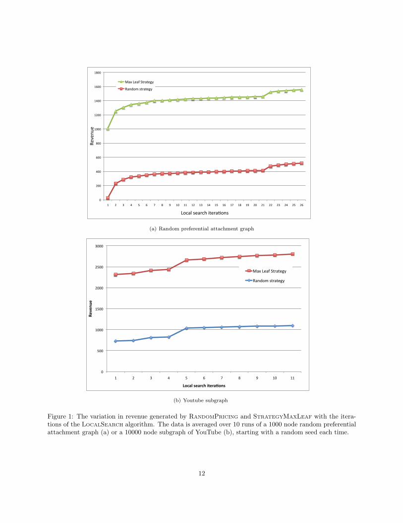
Figure 1: The variation in revenue generated by RANDOMPRICING and STRATEGYMAXLEAF with the itera-tions of the LOCALSEARCH algorithm. The data is averaged over 10 runs of a 1000 node random preferentialattachment graph (a) or a 10000 node subgraph of YouTube (b), starting with a random seed each time.

12

necessarily arbitrary. The result of one particular parameter settings are shown in figure 1(a), which plotsaverage revenue obtained by the two pricing strategies: RANDOMPRICING and STRATEGYMAXLEAF. Eachpoint on the figure is obtained by average revenue over 10 runs on the same graph but with a different(random) seed. The horizontal axis indicates the number of LOCALSEARCH iterations that were done on thegraph, where each iteration consisted of simulating the process 50 times, and choosing the best value overthe runs. It is clear from the graph that STRATEGYMAXLEAF does quite well even without the addition ofLOCALSEARCH, although the addition of LOCALSEARCH does increase the revenue. On the other hand, theRANDOMPRICING strategy performs poorly on its own, but its revenue increases steadily with the iterationsof the LOCALSEARCH algorithm. We note that the difference between the revenue from the two policies doesvary (as expected) with the probability model, and the difference between the revenue is not as large in allthe different runs. But the difference does persist across the runs, especially when the strategies are runwithout the local search improvement.

We also conduct a similar simulation with a real-world network, namely the links between users of thevideo-sharing site YouTube.4 The YouTube network has millions of nodes, and we only study a subset of10, 000 nodes of the network. We simulate the random process as earlier, and the results are shown infigure 1(b). Again, we note that STRATEGYMAXLEAF does very well on its own, easily beating the revenueof RANDOMPRICING. The RANDOMPRICING strategy does improve a lot with LOCALSEARCH, but it fails toequalize the revenue of STRATEGYMAXLEAF. The large size of the YouTube graph and the expensive natureof the LOCALSEARCH algorithm restrict the size of the experiments we can conduct with the graph, butthe results from the above does experiments do offer some insights. In particular, STRATEGYMAXLEAF

succeeds in extracting a good portion of the revenue from the graph, if we consider the revenue obtainedfrom STRATEGYMAXLEAF combined with LOCALSEARCH based improvements to be the benchmark. Further,LOCALSEARCH can improve the revenue from any strategy by a substantial margin, though it may not be ableto attain enough revenue when starting with a sub-optimal strategy such as RANDOMPRICING. Finally, weobserve that the combination of STRATEGYMAXLEAF and LOCALSEARCH generates the best revenue amongour strategies, and it is an open question as to whether this is the optimal adaptive strategy.

5 Conclusions

In this work, we discussed pricing strategies for sellers distributing a product over social networks throughviral marketing. We show that computing the optimal (one that maximizes expected revenue) non-adaptivestrategy for a seller is NP-Hard. In a positive result, we show that there exists a non-adaptive strategyfor the seller which generates expected revenue that is within a constant factor of the expected revenuegenerated by the optimal adaptive strategy. This strategy is based on an influence-and-exploit policy whichcomputes a max-leaf spanning tree of the graph, and offers the product to the interior nodes of the spanningtree for free, later on exploiting this influence by extracting its profit from the leaf nodes of the tree. Theapproximation guarantee of the strategy holds for fairly general conditions on the probability function.

6 Open Questions

The added dimension of pricing to influence maximization models poses a host of interesting questions, manyof which are open. An obvious direction in which this work could be extended is to think about influencemodels stronger than the model examined here. It is also unclear whether the assumptions on the functionC(·) are the minimal set that is required, and it would be interesting to remove the assumption that thereexists a price at which the probability of acceptance is 1. A different direction of research would be toconsider the game-theoretic issues involved in a practical system. Namely, in the model presented here, wethink of each buyer as just sending the recommendations to all its friends and ignore the issue of any “cost”involved in doing so, thereby assuming all the nodes to be non-strategic. It would be very interesting to

4The network can be freely downloaded; see [11] for details.

13

model a system where the nodes were allowed to behave strategically, trying to maximize their payoff, andcharacterize the optimal seller strategy (especially w.r.t. the cashback) in such a setting.

7 Acknowledgments

Supported in part by NSF Grant ITR-0331640, TRUST (NSF award number CCF-0424422), and grants fromCisco, Google, KAUST, Lightspeed, and Microsoft. The third author is grateful to Mukund Sundararajanand Jason Hartline for useful discussions.

References

[1] David Arthur and Sergei Vassilvitskii. k-means++: the advantages of careful seeding. In SODA ’07:Proceedings of the eighteenth annual ACM-SIAM symposium on Discrete algorithms, pages 1027–1035,Philadelphia, PA, USA, 2007. Society for Industrial and Applied Mathematics.

[2] P. Domingos and M. Richardson. Mining the network value of customers. Proceedings of the seventhACM SIGKDD international conference on Knowledge discovery and data mining, pages 57–66, 2001.

[3] M.R. Garey and D.S. Johnson. Computers and Intractability: A Guide to the Theory of NP-Completeness. WH Freeman & Co. New York, NY, USA, 1979.

[4] J. Hartline, V. Mirrokni, and M. Sundararajan. Optimal Marketing Strategies over Social Networks.Proceedings of the 17th international conference on World Wide Web, 2008.

[5] D. Kempe, J. Kleinberg, and E. Tardos. Maximizing the spread of influence through a social network.Proceedings of the ninth ACM SIGKDD international conference on Knowledge discovery and datamining, pages 137–146, 2003.

[6] J. Kleinberg. Cascading Behavior in Networks: Algorithmic and Economic Issues. In N. Nisan,T. Roughgarden, E. Tardos, and V.V. Vazirani, editors, Algorithmic Game Theory. Cambridge Uni-versity Press New York, NY, USA, 2007.

[7] D.J. Kleitman and D.B. West. Spanning Trees with Many Leaves. SIAM Journal on Discrete Mathe-matics, 4:99, 1991.

[8] J. Leskovec, A. Singh, and J. Kleinberg. Patterns of influence in a recommendation network. Pacific-AsiaConference on Knowledge Discovery and Data Mining (PAKDD), 2006.

[9] Jure Leskovec, Lada A. Adamic, and Bernardo A. Huberman. The dynamics of viral marketing. ACMTrans. Web, 1(1):5, 2007.

[10] H.I. Lu and R. Ravi. Approximating Maximum Leaf Spanning Trees in Almost Linear Time. Journalof Algorithms, 29(1):132–141, 1998.

[11] A. Mislove, M. Marcon, K.P. Gummadi, P. Druschel, and B. Bhattacharjee. Measurement and analysis ofonline social networks. In Proceedings of the 7th ACM SIGCOMM conference on Internet measurement,pages 29–42. ACM New York, NY, USA, 2007.

[12] MEJ Newman, DJ Watts, and SH Strogatz. Random graph models of social networks, 2002.

[13] BBC News. Facebook valued at $15 billion. http://news.bbc.co.uk/2/hi/business/7061042.stm,2007.

14

[14] Erick Schonfeld. Amiando makes tickets go viral and wid-getizes event management. http://www.techcrunch.com/2008/07/17/amiando-makes-tickets-go-viral-and-widgetizes-event-management-200-discount-for-techcrunch-readers/,2008.

[15] R. Solis-Oba. 2-Approximation Algorithm for finding a Spanning Tree with Maximum Number of leaves.Proceedings of the Sixth European Symposium on Algorithms, pages 441–452, 1998.

[16] Wikipedia. The beacon advertisement system. http://en.wikipedia.org/wiki/Facebook Beacon,2008.

[17] Wikipedia. Facebook revenue in 2008. http://en.wikipedia.org/wiki/Facebook, 2008.

8 Appendix

8.1 Hardness of finding the optimal strategy

In this section, we show that Problem 1 is NP-hard even for a very simple buyer model M by a reductionfrom vertex cover with bounded degree (see [3] for the hardness of bounded-degree vertex cover). Letting ddenote the degree bound, and letting p = 1

4d , we will use an Independent Cascade Model ICMC with:

C(x) =

1 if x < p,0 if x ≥ p

Intuitively, the seller has to partition the nodes into “free” nodes and “full-price” nodes. In the formercase, nodes are offered the product for free, and they accept it with probability 1 as soon as they receivea recommendation. In the latter case, nodes are offered the product for price 1, and they accept eachrecommendation with probability p. (Note that the seller is allowed to use other prices between 0 and 1 buta price of 1 is always better.)

We are going to use a special family of graphs illustrated in Figure 2. The graph consists of four layers:

• A singleton node s, which we will use as the only initially active node (i.e., S0 = s);

• s links to a set of n nodes, denoted by V1;

• Nodes in V1 also link to another set of nodes, denoted by V2. Each node in V1 will be adjacent to dnodes in V2, and each node in V2 will be adjacent to 2 nodes in V1 (so |V2| = dn/2);

• Each node v ∈ V2 also links to k = 20d new nodes, denoted by Wv; these k nodes do not link to anyother nodes. The union of all Wv’s is denoted by V3.

We first sketch the idea of the hardness proof. The connection between V1 and V2 will be decided by thevertex cover instance: given a vertex cover instance G′(V,E) with bounded degree d, we construct a graphG as above where V1 = V and V2 = E, adding an edge between V1 and V2 if the corresponding vertex isincident to the corresponding edge in G′. The key lemma is that, in the optimal pricing strategy for G, thesubset of nodes in V1 that are given the product for free is the minimum set that covers V2 (i.e., a minimumvertex cover of G′).

To formalize this, first note that, in an optimal strategy, all nodes in V3 should be full-price. Giving theproduct to them for free gets 0 immediate revenue, and offers no long-term benefit since nodes in V3 cannotrecommend the product to anyone else. If the nodes are full-price, on the other hand, there is at least achance at some revenue.

On the other hand, we show the optimal strategy must also ensure each vertex in V2 eventually becomesactive with probability 1.

15

V1 V2

s

...

...

...

...

V3

vu Wv

Figure 2: Reducing Bounded-Degree Vertex Cover to Optimal Network Pricing

Lemma 7. In an optimal strategy, every node v ∈ V2 is free, and can be reached from s by passing throughfree nodes.

Proof. Suppose, by way of contradiction, that the optimal strategy has a node v ∈ V2 that does not satisfythese conditions. Let u1 and u2 be the two neighbors of v in V1, and let q denote the probability that veventually becomes active.

We first claim that q < 2dp. Indeed, if v is full-price, then even if u1 and u2 become active, the probabilitythat v becomes active is 1− (1−p)2 < 2p. Otherwise, u1 and u2 are both full-price. Since u1 and u2 connectto at most 2d edges other than v, the probability that one of them becomes active before v is at most1− (1− p)2d < 2dp. Thus, q < 2dp.

It follows that the total revenue that this strategy can achieve from u1, v, and Wv is 2+kqp < 2+2kdp2 =4.5. Conversely, if we make u1 and v free, we can achieve kp = 5 revenue from the same buyers. Furthermore,doing this cannot possibly lose revenue elsewhere, which contradicts the assumption that our original strategywas optimal.

It follows that, in an optimal strategy, all of V3 is full-price, all of V2 is free, and every node in V2 isadjacent to a free node in V1. It remains only to determine C, the nodes in V1, that an optimal strategyshould make free. At this point, it should be intuitively clear that C should correspond to a minimumvertex-cover of V2. We now formalize this as follows:

Lemma 8. Let C denote the set of free nodes in V1, as chosen by an optimal strategy. Then C correspondsto a minimum vertex cover of G′.

Proof. As noted above, every node in V2 must be adjacent to a node in C, which implies C does indeedcorrespond to a vertex cover in G′.

Now we know an optimal strategy makes every node in V2 free, and every node in V3 full-price. Oncewe know C, the strategy is determined completely. Let xC denote the expected revenue obtained by thisstrategy. Since all nodes in V2 are free and are activated with probability 1, we know the strategy achieves0 revenue from V2 and p|V3| expected revenue from V3.

Among nodes in V1, the strategy achieves 0 revenue for free nodes, and exactly 1− (1− p)d+1 expectedrevenue for each full-price node. This is because each full-price node is adjacent to exactly d+1 other nodes,and each of these nodes is activated with probability 1. Therefore, xC = (|V1| − |C|)(1− (1− p)d+1) + p|V3|,which is clearly minimized when C is a minimum-vertex cover.

Therefore, optimal pricing, even in this limited scenario, can be used to calculate the minimum-vertexcover of any bounded-degree graph, from which NP-hardness follows.

Theorem 2. Two Coupon Optimal Strategy Problem is NP-Hard.

16