Primitive Variable Solvers for Conservative General Relativistic

Magnetohydrodynamics

Scott C. Noble

Physics Department, University of Illinois, Urbana, IL 61801, U.S.A.

scn@uiuc.edu

and

Charles F. Gammie

Physics Department, University of Illinois, Urbana, IL 61801, U.S.A.

gammie@uiuc.edu

and

Jonathan C. McKinney

Harvard-Smithsonian Center for Astrophysics, Cambridge, MA 02138, U.S.A.

jmckinney@cfa.harvard.edu

and

Luca Del Zanna

Dipartimento di Astronomia e Scienza dello Spazio Universita degli Studi di Firenze,

Firenze, Italy

ldz@arcetri.astro.it

ABSTRACT

Conservative numerical schemes for general relativistic magnetohydrodynam-

ics (GRMHD) require a method for transforming between “conserved” variables

such as momentum and energy density and “primitive” variables such as rest-

mass density, internal energy, and components of the four-velocity. The forward

transformation (primitive to conserved) has a closed-form solution, but the in-

verse transformation (conserved to primitive) requires the solution of a set of five

nonlinear equations. Here we discuss the mathematical properties of the inverse

– 2 –

transformation and present six numerical methods for performing the inversion.

The first method solves the full set of five nonlinear equations directly using a

Newton-Raphson scheme and a guess from the previous timestep. The other

methods reduce the five nonlinear equations to either one or two nonlinear equa-

tions that are solved numerically. Comparisons between the methods are made

using a survey over phase space, a two-dimensional explosion problem, and a

general relativistic MHD accretion disk simulation. The run-time of the methods

is also examined. Code implementing the schemes is available for download on

the web.

Subject headings: hydrodynamics — methods: numerical — MHD

1. Introduction

It is commonly thought that many astrophysical systems contain relativistic plasmas

with a dynamically significant magnetic field. Examples include accreting black holes in

black hole binaries, galactic nuclei, gamma-ray bursts, the cores of massive stars undergoing

core collapse, isolated neutron stars, and neutron stars in binary systems.

As a result, there is currently considerable interest in numerical methods for integrating

the equations of general relativistic magnetohydrodynamics (GRMHD). Within the last few

years about six GRMHD schemes have been deployed (Komissarov 2005; Koide, Shibata, &

Kudoh 1999; Gammie, McKinney, & Toth 2003; De Villiers & Hawley 2003; Fragile 2005;

Duez et al. 2005; Anton et al. 2005).

Some of these authors (Komissarov 2005; Koide, Shibata, & Kudoh 1999; Gammie,

McKinney, & Toth 2003; Duez et al. 2005; Anton et al. 2005) have adopted a conservative

scheme. This means that the integrated equations are of the form

∂tU(P) = −∂iFi(P) + S(P) (1)

Here U is a vector of “conserved” variables, such as particle number density, or energy or

momentum density in the coordinate frame, the Fi are the fluxes, and S is a vector of source

terms that do not involve derivatives of P and therefore do not affect the characteristic

structure of the system. U is conserved in the sense that, if S = 0, the rate of change of the

integral of U over the volume depends only on fluxes at the boundaries, by the divergence

theorem. The vector P is composed of “primitive” variables such as rest-mass density,

internal energy density, velocity components, and magnetic field components. The fluxes

and conserved quantities depend on P. Conservative numerical schemes advance U, then

depending on the order of the scheme, calculate P(U) once or twice per timestep.

– 3 –

In nonrelativistic conservative MHD schemes the conserved quantities are trivially re-

lated to the primitive variables; both the forward transformation P → U and the inverse

transformation U → P have a closed-form solution. In GRMHD (or even SRMHD) U(P)

is a complicated, nonlinear relation. The inverse transformation has no closed-form solution

and must be performed numerically. This numerical operation must be robust, accurate,

and fast—it is at the heart of all conservative GRMHD schemes.

In this paper we investigate several schemes for the inversion P(U) and test each in

an axisymmetric simulation of accretion onto a rotating black hole. § 2 covers definitions

and notational matters. § 3 describes five distinct formulations of the algebraic equations

to be solved numerically, and § 4 describes how each method is implemented numerically.

§ 5 describes the performance of these methods in the context of a survey over a range of

primitive variable values and in two typical applications. § 6 summarizes our findings and

contains a guide to our results for those wishing to make their own implementation. We will

assume throughout that G = c = 1.

2. Definitions

Throughout this paper we follow standard notation (Misner, Thorne, & Wheeler 1970).

We work in a coordinate basis with metric components gµν and independent variables

t, x1, x2, x3. The normal observer’s four-velocity is nµ = (−α, 0, 0, 0) in this coordinate

basis, where α2 = −1/gtt is the square of the lapse.

The fluid is described by its four-velocity uµ, rest-mass density ρ◦, internal energy per

unit (proper) volume u, and pressure p. The electromagnetic field is described by the field

tensor F µν , which is antisymmetric, and its dual

∗

Fµν

=1

2εµνκλFκλ. (2)

The field tensor has six degrees of freedom (three components each for E and B), but three

are eliminated by the ideal MHD condition

uµFµν = 0 (3)

which states that the Lorentz force vanishes in the rest-frame of the fluid. It is convenient

to describe the field using the magnetic field four-vector

Bµ ≡ −nν∗

Fµν

. (4)

Notice that Bµnµ = 0 and the vector B differs from the magnetic field variables

Bi ≡ ∗

Fit

=Bi

α(5)

– 4 –

that we have used in earlier papers in this series (Gammie, McKinney, & Toth 2003; Gammie,

Shapiro, & McKinney 2004; McKinney & Gammie 2004). It is also useful to define the

projection tensors

hµν = gµν + uµuν (6)

which projects into a space normal to the fluid four-velocity uµ and

jµν = gµν + nµnν (7)

which projects into the space normal to the normal observer nµ.

The governing equations for GRMHD are conservation of stress-energy,

T µν;µ = 0 (8)

conservation of particle number,

(ρ◦uµ);µ = 0, (9)

and the homogeneous Maxwell equations

∗

Fµν

;ν = 0. (10)

Often, we will assume a Γ-law gas, with equation of state

p = (Γ − 1) u. (11)

Some (but not all) of the schemes described here do not work for other equations of state.

We will note where our assumed equation of state is essential.

The GRMHD stress-energy tensor is

T µν =(

w + b2)

uµuν +

(

p +b2

2

)

gµν − bµbν. (12)

Here

w = ρ◦ + p + u, (13)

b2 = bµbµ, and

bµ =1

γhµ

νBν , (14)

where

γ ≡ −nµuµ (15)

is the Lorentz factor of the flow as measured in the normal observer frame; in our coordinate

basis γ = αut.

– 5 –

There are many possible choices of conserved and primitive variables. For definiteness,

we will make a specific choice that is nearly identical to that used in the HARM code

(Gammie, McKinney, & Toth 2003). Once an inversion scheme is found for this particular

set many other choices can be obtained by simple algebraic transformations.

For primitive variables, we use ρ◦, u,Bi, and ui ≡ jiµu

µ (ut = 0). These velocities are

the projection of the plasma four-velocity into the space perpendicular to nµ. They can be

rewritten ui = ui+αγgti, or, in the language of the ADM (Arnowitt-Deser-Misner) formalism

ui = ui +γβi/α, where βi = α2gti is the “shift”. The uis are numerically convenient because

they range from −∞ to ∞.

For conserved variables, it is helpful to first write out the basic equations in full. The

equations of energy-momentum conservation are

∂t

(√−gT tµ

)

+ ∂i

(√−gT iµ

)

=√−gT κ

λΓλνκ, (16)

where g ≡ Det(gµν). The associated conserved variables are√−gT t

µ. It is convenient to

convert these to

Qµ ≡ −nνTνµ = αT t

µ, (17)

which is the energy-momentum density in the normal observer frame.

The Maxwell equations yield three evolutionary equations

∂t

(√−gBi)

= −∂j

[√−g(

bjui − biuj)]

(18)

and the constraint

∂i

(√−gBi

)

= 0, (19)

which does not concern us here.

The particle number conservation equation is

∂t

(√−gρ◦u

t)

= −∂j

(√−gρ◦u

j)

. (20)

The conserved variable for this equation is√−gρ◦u

t. It is convenient to convert this to

D ≡ −ρ◦nµuµ = ρ◦αut = γρ◦ . (21)

This is the density measured in the normal observer frame.

To sum up, the eight conserved variables are Qµ, D, and Bi. We are now in a position

to give explicit expressions for the forward transformation U(P).

– 6 –

First, we calculate p = (Γ − 1) u, w = ρ◦+u+p, γ =√

1 + gijuiuj, uµ = (γ/α, ui − αγgti),

and bµ = hµνBν/γ. Then

D = γρ◦, (22)

Qµ = γ(

w + b2)

uµ −(

p + b2/2)

nµ + (nνbν) bµ, (23)

and of course the Bis are both primitive and conserved variables. Along the way, it is

computationally efficient to use the identities

b2 =1

γ2

[

B2 + (Bµuµ)2] (24)

and

nµbµ = −uµBµ. (25)

The next section will show how these equations are used to perform the inverse transforma-

tion.

3. Inversion Schemes

No closed-form inversion of (22,23) from D, Qµ to the primitive variables ρ◦, u, ui is

known, so the primitive variables must be found numerically. In this section, we describe

and discuss several methods for solving these equations.

A popular and robust means of solving systems of algebraic equations numerically is

the Newton-Raphson (NR) scheme (see Section 9.6 of Press et al. (1992)). Since it is also

simple to code, we will employ this method by default.

3.1. 1DW Scheme

It seems likely that the solution would be obtained more efficiently if one could manipu-

late the five fundamental equations to reduce the dimensionality of the system, as was done

by Del Zanna, Bucciantini, & Londrillo (2003) for special relativistic MHD. Our procedure

for reducing the 5D system is to evaluate certain scalars from the conserved variables, then

expand expressions for these scalars to simplify the solution. We will use D, QµBµ, and

Qµnµ, which is the energy density measured in the normal observer frame. We will also use

Q2, where Qν = jνµQµ, which is the energy-momentum flux perpendicular to the normal

observer. Ultimately, we obtain two equations dependent only on the known conserved vari-

ables and two independent variables γ and w. Instead of these two unknowns, however, we

use W ≡ wγ2 and v2 ≡ vivi, where vi = ui/γ is the flow velocity relative to the normal

– 7 –

observer. These new variables simplify the equations and lead to numerical schemes that are

more robust. Whenever γ is stated from now on, it is implied that it is calculated from v2

via the identity γ2 = 1/ (1 − v2).

A consistent procedure can be developed as follows. First, expand the definition of Qµ

to find the key result

BµQµ = (uµBµ) W/γ. (26)

Since BµQµ can be evaluated in terms of the (known) conserved variables, this equation can

be used to eliminate uµBµ in favor of the unknowns v2 and W .

Next, expand Q2 using (26) to find

Q2 = v2(

B2 + W)2 − (QµBµ)2 (B2 + 2W )

W 2. (27)

Finally, we solve for v2 to find the simple result

v2 =Q2W 2 + (QµBµ)2 (B2 + 2W )

(B2 + W )2 W 2. (28)

This is the relativistic counterpart of the nonrelativistic expression v2 = P 2/ρ2, where P is

the magnitude of the momentum density vector ρv. It gives us an explicit expression for

v2(W ) that results in positive definite evaluations if implemented in the code as shown here.

Next, expand Qµnµ using (26) and the variables γ and W :

Qµnµ = −B2

2

(

1 + v2)

+(QµBµ)2

2W 2− W + p(u, ρ◦). (29)

This remaining equation then yields a solution for W . Specifically, the 1DW scheme solves

one nonlinear algebraic equation (29), which is now only a function of W since (28) is used

to eliminate v2.

Once v2 and W are found one can recover w, ρ◦ (from D), and u. The next step is to

find ui using Qi. After some manipulation one finds

Qµ =1

γ

(

W + B2)

uµ − (uνBν)Bµ

γ. (30)

Since uµBµ = (γ/W )(QµBµ), this can be used to solve for ui:

ui =γ

W + B2

[

Qi +(QµBµ)Bi

W

]

(31)

– 8 –

3.2. 2D Scheme

The equation to be solved in the 1DW method includes a quotient of polynomials in

W since it implicitly uses (28) for v2. This suggests that numerical pathologies might arise

near roots. By solving the two, simpler equations (27,29) simultaneously for W and v2, one

may eliminate such problems. We call this method the 2D scheme since it involves solving

a two-dimensional algebraic system.

We find that using v2 instead of u2 or γ is particularly advantageous for this method.

This is because equations (27,29) are linear only in v2 (modulo the v2-dependence of the state

equation) and not in u2 or γ. The linear dependence on v2 increases the rate of convergence

for this quantity and is guaranteed to be well-behaved in the vicinity of a root.

Koide et al. (1996) and Koide, Shibata, & Kudoh (1999) also used a two-dimensional

method. But instead of v2 and W , they use (γ − 1) and (uµBµ) as independent variables.

We have not tried their method since the functions they minimize are more complicated than

ours and assume a Γ-law state equation. Further, it is likely that these two methods would

perform similarly since one can eliminate W for uµBµ in our method via equation (26). As

mentioned earlier, we find better performance using v2 instead of γ.

3.3. 5D Scheme

The simplest procedure, and the one we used initially in the HARM code, is to invert

the five equations (22) to (23) using a multidimensional NR scheme. This requires evaluating

the matrix of derivatives ∂U/∂P. Further, a Newton iteration of this system involves more

operations than the 1DW and 2D schemes since it requires calculating elements of ∂U/∂P

and a matrix inversion. Also, we find that it requires an initial guess that is close to the

solution. This is almost always available from the last timestep (and if the guess is not good

it usually means something is wrong). Because it involves root-finding in a five-dimensional

space we call this the 5D scheme. The conserved variables used in this method are the same

as those used in Gammie, McKinney, & Toth (2003). All other methods described here use

D and Qµ.

Notice that the 1DW , 2D, and 5D schemes do not require a particular equation of state.

For example, derivatives of p with respect to the independent variables could be obtained

from equation of state tables using finite difference approximations. Two of the next three

methods, however, assume a Γ-law equation of state.

– 9 –

3.4. 1Dv2 and 1D?v2 Schemes

Another scheme can be derived if we assume that the equation of state is

p = (Γ − 1) u =Γ − 1

Γ

(

w − D

γ

)

. (32)

If we make this substitution and use the expression for v2(W ), equation (29) reduces to an

eighth-order polynomial in W , for which there is no general closed-form solution according to

the theorem of Abel-Ruffini. It is simplest to solve this single nonlinear equation numerically.

Because of the complexity introduced by the equation of state there is likely no general way

of isolating the physical root, and one must simply look for a solution that is close to the

solution of the last timestep. With other state equations, it may not be possible to express

(29) in polynomial form at all.

It is worth noting how this situation resolves itself in relativistic hydrodynamics. Equa-

tion (28) becomes

u2 =Q2

W 2 − Q2(33)

and equation (29) becomes

Qµnµ = p(W, D/γ) − W. (34)

Obviously, there is no general solution since one has the freedom of choosing an equation

of state. Our particular equation of state, however, yields a quartic whose solution was

discussed by Eulderink & Mellema (1995).

Instead of solving the eighth-order polynomial directly, the 1D v2 scheme, which is a

modified version of the special relativistic method described in Del Zanna, Bucciantini, &

Londrillo (2003), solves a cubic equation for W (u2) and a nonlinear equation for u2. The

cubic described in Del Zanna, Bucciantini, & Londrillo (2003), however, can sometimes have

two positive, real solutions for W . The larger root appears to be the physical one, though

a general proof of this has eluded us. In order to eliminate this uncertainty, we use the

following cubic equation which we have proved leads to only one, positive solution1

C(W ) = W 3 + 3d2W2 − 4d0 = 0 (35)

where

d0 ≡Γ (QµBµ)2

8 [1 + v2 (Γ − 1)], (36)

1The signs of the cubic solutions can be derived from the locations of the cubic’s local extrema. The

existence of only one positive solution stems from the following properties of the cubic: 1) ∂C/∂W |W=0 = 0;

2) C(W = 0) ≤ 0 always; and 3) limW→±∞ C(W ) = ±∞.

– 10 –

d2 ≡Γ

3 [1 + v2 (Γ − 1)]

[

Qµnµ +B2

2

(

1 + v2)

+ D (1 − 1/Γ)√

1 − v2

]

. (37)

Equation (35) results from multiplying equation (29) by ΓW 2/ [1 + v2 (Γ − 1)] and sub-

stituting equation (32) for p(W, D/γ). In general, there are three solutions which are given

in closed-form by Cardano’s formula (Weisstein 2004; Rade and Westergren 1990). If our

cubic has a positive and real solution then there is only one positive and real solution, and

it can be shown that this solution is always equal to the following

W = −d2 +(

2d0 − d32 +

√D

)1/3

+(

2d0 − d32 −

√D

)1/3

, (38)

where

D ≡ 4d0

(

d0 − d32

)

. (39)

It is useful to know that d0 ≥ 0 always and d2 can take negative and positive values. When

D < 0, the solution can be expressed in a simpler form:

W (D < 0) = d2 [cos (θ/3) − 1] , θ = cos−1[

2d0/d32 − 1

]

. (40)

Table 1 lists the possible physical solutions of (35) depending on the particular values of d0

and d2. In the 1Dv2 scheme, we use the physical solution for W (v2) and numerically solve an

equation proportional to equation (27) for v2. That is, 1Dv2 solves for v2 via a NR method

in which the physical cubic solution is calculated for each iteration.

One drawback of this method is that it requires that the state equation be linear in

W . Solving equation (29) numerically instead makes the method compatible with general

equations of state. We call this technique the 1D ?v2 scheme. It consists of taking NR

iterations to find W (v2) nested within Newton iterations to find v2. In other words, for each

Newton update of v2, we solve equation (29) for W using a separate NR method assuming the

most current value for v2. This supplies the next v2 iteration with a consistent value for W .

Surprisingly, this nested NR method (1D?v2) is faster, more robust and more accurate than

the 1Dv2 method. The difference in accuracy and efficiency is likely due to the appearance

of transcendental functions and condition statements in the closed-form solution of (35).

3.5. Polynomial Scheme

The substitution of equation (28) into equation (29) leads to an eighth-order polynomial

in W if we assume a Γ-law equation of state (32). This suggests the possibility of using a

– 11 –

general polynomial root-finding method (such as Numerical Recipes’ zroots) that finds all

8 roots. We will call this the polynomial scheme.

The physical root can be identified by requiring that it also solve the five equations U =

U(P). Unfortunately this test can sometimes yield ambiguous results due to amplification

of roundoff error, making it difficult to identify the correct solution. This method also turns

out to be computationally expensive.

4. Numerical Implementations

In the previous section, we described the mathematical framework that embodies the

primitive variable inversion methods we have tested. We will now discuss the details of the

numerical methods we have used to test the performance of these formulations. All routines

(in the C language) are available for download from the web.2

We use the Newton-Raphson scheme to solve the nonlinear algebraic equations of the

1DW , 2D, 5D, 1D?v2 , and 1Dv2 methods. An excellent description of this method—as well as

other root-finding methods—can be found in Press et al. (1992); we will only state unique

aspects of our implementation here and defer further explanation to our source code. Let

R denote the system of nonlinear equations, or “residuals,” x the independent variables

for which we are solving, and J the Jacobian whose (i, j)-component is ∂Ri/∂xj. The NR

procedure assumes that R is smooth and nearly linear, so that we can make consecutive

linear corrections to our guess that lead us toward the root. This NR step is defined as the

following:

∆x = −J−1 · R . (41)

We measure convergence using a “Newton-Raphson error function,” ENR = |∆W/W |,where ∆W is the change in W between the two most recent NR iterations. We find that

other convergence criteria yield little if any improvement, which is not surprising since W

is the crucial variable. In particular, a convergence criterion based on residual errors in

the solution of equations (22,23) is not used for any of the schemes since it is difficult to

normalize the error properly a priori over the entire parameter space.

The condition for stopping the iterative procedure involves three parameters: TOL, NNR

2The current version of the source code for each method described in this paper can be

found in the electronic edition of the Journal, while a maintained version can be obtained at

http://rainman.astro.uiuc.edu/codelib/codes/pvs grmhd/. The methods can be used with any user-supplied

spacetime metric.

– 12 –

and Nextra. If ENR falls below TOL after performing at least one iteration, then only Nextra

more iterations are performed. A solution is said to be found if the tolerance criterion is

satisfied before NNR iterations.

The impetus for the additional Nextra iterations is one of efficiency and accuracy. When

the error reaches our tolerance level, the extra iterations try to reduce it even further. Since

this can sometimes be fruitless—e.g. the solution error becomes insensitive to subsequent

NR steps—we set Nextra to a small number. The parameters used by default in this paper are

TOL = 10−10 and Nextra = 2, which should yield solutions accurate to within roundoff error if

the guess is sufficiently near the true solution, since the NR method converges quadratically.

What value should be chosen for TOL? Ideally the inversion error TOL should be smaller

than the truncation error that is inevitably introduced in the numerical evolution of U. But

truncation error is difficult to estimate on-the-fly 3 and cannot usually be estimated a priori.

Different problems may require different values of TOL. One class of problems that is

particularly sensitive to the value of TOL is the evolution of small amplitude waves. This is a

problem of some interest, as it is frequently used in convergence testing numerical methods.

In this case the fluctuating part of the fluid variables is small, and the truncation error is

a small fraction of that. The truncation error can therefore be a very small fraction of the

conserved variables, and TOL must be comparably small to avoid spoiling convergence. On

the other hand, the measurements of the accretion rates of rest mass, energy, and angu-

lar momentum in the relativistic disk simulation discussed below appear to be peculiarly

insensitive to TOL. The only safe course is to directly check the sensitivity of numerical

measurements to TOL.

During a sequence of NR iterations, an independent variable may leave its allowed do-

main (e.g. superluminal velocities). In order to prevent numerical divergences and unwanted

imaginary parts, we reset the independent variable to a value in its physical domain. For

example, in the 1DW , 1Dv2 , 1D?v2 , 2D and polynomial methods, we demand that 0 < v2 < 1

and W > 0. No constraints are used in the 5D method, since experimentation with this has

led us to believe that constraining ρ◦, u > 0 only increases the likelihood of not converging

to a solution.

A special note on the polynomial scheme, where we use Laguerre’s method to find W :

there is an additional numerical criterion that must be used for evaluating which of the 8

3Local truncation error estimation can be accomplished in place during a simulation without knowing

the exact solution beforehand by solving the equations of motion additionally on a “shadow” grid whose grid

spacing is half that of the base grid. The truncation error estimate is then calculated by comparing the two

solutions at coincident timesteps (Berger & Oliger 1984; Choptuik 1995).

– 13 –

roots is the physical root. One first eliminates roots that have imaginary components above

some threshold value, then evaluates the residuals in the solution of the basic equations for

the remaining roots. The root with the smallest residuals is identified as the physical root.

As for the NR methods, parameters TOL, NNR and Nextra are used to control the accuracy of

the solutions.

A few final comments on numerical implementation. In terms of complexity, the 1DW ,

1D?v2 , 2D, and polynomial methods are the easiest to implement; some care is required in

finding the physical solution to the cubic equation in the 1Dv2 scheme. The lower-dimensional

NR schemes are simple enough to derive the closed-form expressions for R, J and ∆x by

hand, so we have coded those in directly. The 5D scheme, by contrast, is complicated by

the need to evaluate the 25 elements of J. This can be done analytically (this procedure is

time-consuming and prone to error) or numerically using finite differences (this is simple but

introduces additional numerical noise).

5. Tests

The space of possible numerical approaches to the inversion problem is large, so we

can make no claim that any of our methods are optimal or near-optimal. In this section,

through a series of tests, we show that some of the methods are “good enough” in the

sense that (1) they can be shown not to contribute significantly to the numerical error in

actual astrophysical applications, and (2) some of them are efficient enough that they do

not contribute significantly to the computational cost of an evolution. We have expended

significant effort in optimizing each scheme’s speed and accuracy, so that these tests make a

fair comparison between the various methods.

We consider three tests. The first is a parameter space survey in which the primitive

variables are varied over many orders of magnitude and the accuracy of the solution is

evaluated. The second test places the inversion routine in a special relativistic MHD code

and evolves a magnetized, cylindrical explosion problem due to Komissarov. The third test

places the inversion routine in a general relativistic MHD code and evolves a magnetized

disk around a rotating black hole. Throughout we assume a the Γ-law equation of state (32)

with Γ = 4/3.

– 14 –

5.1. Parameter Space Survey

The inversion routine takes as arguments the 8 conserved variables (three are mag-

netic field components and are trivially converted to primitive variables), guesses for the 5

nontrivial primitive variables, and the 10 components of the metric. This parameter space

is too large to cover exhaustively, so we only vary ρ◦, u, B2, γ (the Lorentz factor), and

Φ ≡ cos−1(

uiBi/

√

uiuiBjBj)

over the region spanned by a typical accretion disk evolution:

log10 ρ◦ ∈ [−7, 1] , log10 u ∈ [−10, 0] , log10 γ ∈ [0.002, 2.9] ,

log10 B2 ∈ [−8, 1] , cos Φ ∈ [−1, 1] .(42)

We sample uniformly in the logarithm for each variable. Specifically, 40 × 40 × 20 × 20 × 9

points are evenly sampled along dimensions log10 ρ◦ ⊗ log10 u ⊗ log10 γ ⊗ log10 B2 ⊗ cos Φ,

respectively. In order to choose reasonable relative magnitudes between the components of

ui and Bi at a given location with respect to the Kerr-Schild metric, we select 9 points from

an accretion disk simulation (see Section 5.3) at which cos(Φ) ' −1, . . . , 1. The specific

values of cos(Φ), ui, Bi and coordinates used for the parameter space survey are given in

Table 2. The overall magnitudes of the ui and Bj are set by the values of γ and B2 at the

given parameter space point.

At each point of the parameter space we perform the forward transformation; this gives

a (nearly) exact solution to the inversion. We then feed the inverter a guess obtained by

multiplying each primitive variable by 1 + d, where d is a random value between −1 and 1.

The same sequence of random values is used for each method. This turns out to be quite a

stringent test, particularly when the random value is near −1. Even though the maximum

threshold for the offset may not be large enough to model the behavior at strong shocks,

it is approximately the maximum seen for ρ◦ and u in the bulk flow of our accretion disk

simulations (see Section 5.3).

Our parameter space surveys were made using TOL = 10−10, NNR = 30 and Nextra = 2;

these values were determined after the fact to be nearly optimal.

Figure 1 shows the normalized error in the internal energy, ∆u/u, for all the methods.

These accuracy measurements indicate how strongly roundoff errors are amplified by the

scheme. The error is averaged over all the parameters except u. Only the points for which

all the methods converge are included in the average4. Two methods stand out as less

4Since the 5D method fails at almost half the original points and a majority of these failures occur

when γ is large, this may introduce a bias. We have performed an identical survey in which no points were

neglected. Even though solution rates decrease slightly, the rankings in Table 3 stay the same. The high-ENR

– 15 –

accurate: the polynomial scheme, and the 1Dv2 scheme. An examination of ∆u/u over

the entire parameter space indicates that the the 1DW , 2D and 1D?v2 methods yield almost

indistinguishably accurate solutions. If one ignores failures points, the 5D method is often

as accurate as these methods. The 1Dv2 is the fifth most accurate (ignoring failure points),

and the polynomial scheme is the least accurate.

The relative errors in ρ◦ and ui increase with increasing B2/ρ◦, B2/u, and γ for the

most accurate schemes. The relative error of u—for the same methods—grows with ρ◦/u, γ

and B2/u, and is fairly independent of B2/ρ◦. We find that there is typically a maximum

value of ρ◦/u above which the methods nearly always fail; this maximum value starts large

(∼ 1017) but reaches unity by the time γ ∼ 106 5. We find that poor accuracy (& 1% relative

error) in ρ◦ and ui usually occurs for points with B2/ρ◦, B2/u & 1010, but u is accurate for

B2/u . 1012. The dependency on γ seems to not be strongly tied to any of the other

variables, and we find that—on average—& 1% relative errors are seen when γ & 103 − 106.

Also, the accuracy of all the methods improves as cos Φ → 0, on average. Note that the

precise values of these thresholds are not universal to all situations, and are quantitatively

dependent on all the degrees of freedom, including the offset d.

The inversion routine is said to “fail” if it has not converged after NNR = 30 iterations.

Failure rates for the methods are given in Table 3. Here the 2D method stands out as the

best, failing only 5 times in the survey of 5.76×106 points. The 1DW and 1D?v2 methods also

have low failures rates. The 1Dv2 and polynomial schemes fail much more frequently, at a

rate about an order of magnitude lower than that of the least robust 5D method. Notice that

while the polynomial method converges more often than the 5D method, it often converges

to an inaccurate result.

We have found that all the methods asymptote to a minimum failure rate as the range in

d is diminished, i.e. as δ1 → 0 when d ∈ [−δ1, δ1]. The 5D method’s asymptotic regime ends

at approximately δ1 ' 10−3, while the other methods are insensitive to changes for δ1 < 1,

where δ1 = 1 is the maximum value for which the ρ◦ and u guesses remain non-negative.

If we instead vary the overall magnitude of the guess, i.e. (1 + d) → δ2 (1 + d), set δ1 = 1,

and set δ2 ∈ [10−6, 106], we find that the 5D method has a minimum failure rate at about

tails (Figure 2) extend to larger values of ENR; the ENR distributions of the 2D, 1DW , 1D?

v2 , 1Dv2 and 5D

methods now extend to ∼ 10−10, 10−9, 10−9, > 1 and > 1, respectively. More iterations are required and

all methods but the 2D method have NNR distributions extending to NNR = 30. The 2D method remains

the best method.

5These numbers were obtained in an extended parameter space survey in which we sampled 404 points

for each of the 9 values of Φ over the space log10(ρ◦), log10(u), log10(B2) ∈ [−10, 10] , and log10(γ) ∈ [0, 6].

– 16 –

δ2 ∼ 1 as expected. The other methods fail at different, yet constant, minimum rates up

until δ2 & 100; this may be because the residuals used in these routines steepen as W → ∞.

This does not imply that every time the density jumps by ∼ 103 the method will fail, since

the relative offsets are not likely to be large for all primitive variables at the same time in

practice. The high failure rate and greater sensitivity to the guess’ offset seen with the 5D

method is easily attributed to the fact that higher-dimensional minimization problems are

more difficult than lower-dimensional problems (e.g. Press et al. (1992)); more dimensions

admit residuals with more complicated landscapes and make a method more likely to be

mired by local minima.

As another means of demonstrating the accuracy of each method’s solutions, we show

histograms in Figure 2 of the parameter space points binned against the method’s exit value

of ENR. Any points for which ENR ≤ 10−10 are considered acceptable solutions; since only

those points for which solutions are found by all methods are included, there are no points

beyond ENR = 10−10. Those methods that explicitly solve for W (i.e. 2D and 1DW ) give rise

to a power-law distribution extending up to machine precision since the change in W between

iterations ∆W is explicitly calculated during the NR step. The other methods result in non-

zero ∆W/W only when it is above machine precision since they calculate it by subtracting

the previous iteration’s value from the present one. From a numerical perspective, anything

below machine precision should be considered equivalent to zero anyway, so we shall only

concern ourselves with the distributions above machine precision. In this regime, the 2D

method again yields the best results, followed by 1D?v2 , 1DW , 1Dv2 and 5D in order of

increasing average ENR.

What is the maximum accuracy attainable by each method? We have surveyed param-

eter space using values of TOL = 10−15 and NNR = 200, which should give close to maximum

accuracy. The distributions of ENR for the 1DW , 2D and 1D?v2 methods remained nearly

unchanged from those shown in Figure 2 which used the default (less accurate) set of pa-

rameters; the additional iterations failed to significantly reduce solution error, on average,

for these methods. The 5D method, however, does benefit from a larger NNR. Its accuracy

and failure rate improve the longer it is allowed to iterate, although it still underperforms

the 2D, 1DW and 1D?v2 solvers.

In order to measure how quickly the methods converge to a solution, we have plotted

histograms in Figure 3 of the number of NR iterations, NNR, each method performed before

exiting per parameter space point. From the figure, we see that the 1DW , 2D and 1D?v2

methods all typically use between 6−10 iterations, and that they give rise to nearly Gaussian

distributions in this regime. The 1Dv2 method has an extended power-law tail, while the 5D

method has a nearly constant distribution over NNR. Even though the 1Dv2 scheme has a

– 17 –

peak at small NNR that is narrower and taller than the other schemes—suggesting that it

may be more efficient— it fails to find a solution quite frequently and has a substantial tail.

The 1DW method appears to have the best convergence rate over the sampled parameter

space since it has a steep exponential tail and it usually converges to a solution in less than

10 iterations.

Which scheme is fastest? Table 3 shows the number of solutions per second achieved by

each scheme in the parameter survey, on our 3.06 GHz Intel box. The two fastest methods—

1DW and 2D—are about 30% faster than 1Dv2 method, which also has the smallest average

NNR. Since the 1D?v2 method performs many more computations (because of its nested NR

scheme), it takes fourth place. The 5D method is almost an order of magnitude slower, due

to its larger linear system and larger average NNR. The polynomial method is a factor of 2

slower than the 5D.

We have tried a variety of schemes for improving the accuracy and convergence rate of

each scheme. For the NR schemes, we tried implementing a line searching method, which

attempts to find an optimal step size along the direction of steepest descent (Press et al.

1992). This method saves a few of the nonconvergent outliers in the parameter space survey

for the 1DW method but does not help anywhere else for any other method. We tried this

improved 1DW scheme in an accretion disk simulation and found that it did not improve the

success rate at all in the disk simulation.

To sum up, the 2D method has the lowest failure rate and is only slightly more com-

putationally expensive than the fastest method. If the initial guesses are close enough to

the solution, the 5D and 1Dv2 methods fare nearly as well as the more successful 1DW , 2D,

and 1D?v2 methods in accuracy but because of their larger rates of nonconvergence neither is

recommended. The polynomial method is slow and inaccurate, and we do not recommend

it. We will ignore the worst of these methods in the next two sections and discuss the

performance of only four methods: 2D, 1DW , 1D?v2 , and 5D.

5.2. Cylindrical Explosion

The parameter space survey may emphasize different aspects of the inversion routine

than a realistic RMHD problem. Here we consider inversion routine performance in a special

relativistic, slab-symmetric, magnetized explosion. We use the same initial conditions as

Komissarov (1999). The computational domain is defined in Cartesian coordinates (x, y) ∈[−6, 6] × [−6, 6] discretized by 200 × 200 points. A pressure-enhanced cylinder is centered

on the origin with radius r = 0.8, and is matched exponentially to a constant background

– 18 –

that starts at r = 1. The inner state has ρ◦(r < 0.8) = 10−2 and P (r < 0.8) = 1, while

the outer state is initialized with ρ◦(r > 1) = 10−4 and P (r > 1) = 3 × 10−5. All spatial

components of the velocity are zero at t = 0, and the magnetic field is uniform, pointing in

the x-direction: Bµ = (0, 0.1, 0, 0).

We evolved the initial state using a version of the HARM (Gammie, McKinney, & Toth

2003) code. We use an HLL (Harten et al. 1983) flux, and linear (second order) reconstruction

with a minmod slope limiter. We use a Courant factor of 0.1 in the evolution. Figure 4 is

a reconstruction of Figure 10 of Komissarov (1999) using our own evolution; the results are

qualitatively identical.

All the inversion schemes perform similarly on this problem. Table 4 outlines the speed

and failure rates obtained with each method. When a solution is found, it is found by all

methods in less than 10 iterations. The only significant differences are in the run time: the

2D is clearly fastest, while 5D is a factor of 2 slower than the next fastest method. The failure

rates are the same, because the methods fail at the same points where the U calculated from

the evolution is unphysical. The small Courant factor may play a role in the low failure rate

here, since smaller timesteps imply smaller changes in the U over a timestep, so the initial

guess used in the inversion routine (P from the previous timestep) is closer to the solution.

5.3. Accretion Disk Evolution

A more challenging context for testing the inversion routines is the evolution of a magne-

tized, centrifugally supported torus around a Kerr black hole (see, e.g., McKinney & Gammie

(2004) and Gammie, Shapiro, & McKinney (2004) for similar applications). In this particular

incarnation of the problem we evolve a Fishbone & Moncrief (1976) torus containing a weak

poloidal seed field around a Kerr black hole with a/M = 0.9375. The initial state is unstable

to the magnetorotational instability (Balbus & Hawley 1991), so turbulence develops in the

disk and material accretes onto the black hole.

The inner edge of the initial torus lies as 6GM/c2 and the pressure maximum lies

at 12GM/c2. The Fishbone-Moncrief equilibrium condition of uφut = 4.28 is used. On

top of the Fishbone-Moncrief torus we add a weak magnetic field with vector potential

Aφ = Max (ρ◦/ρmax − 0.2, 0) where ρmax is the maximum of the disk’s rest-mass density.

The magnetic field amplitude is normalized so that ratio of gas to magnetic pressure within

the disk has a minimum of 100. With the addition of the field the disk is no longer strictly

in equilibrium, but it is only weakly perturbed.

The initial conditions are evolved using the HARM code. The flux is a local Lax-

– 19 –

Friedrichs flux, and linear (second order) interpolation is used with a Monotonized Central

limiter. Since HARM is incapable of evolving a perfect vacuum, we surround the disk in an ar-

tificial atmosphere, or “floor” state, with ρ◦,atm = 10−4(r/M)−3/2 and uatm = 10−6(r/M)−5/2.

Also, ρ◦ and u are set to their floor values if and when they fall below the floor at any point

in the evolution.

The equations of motion are solved using finite difference approximations on a dis-

crete domain of so-called Modified Kerr-Schild (MKS) coordinates. Instead of the stan-

dard Kerr-Schild coordinates (t, r, θ, φ), a uniform discretization of MKS coordinates xµ =

(t, x(1), x(2), φ) is used where

r = ex(1)

, θ = πx(2) +1

2(1 − h) sin(2πx(2)) . (43)

This coordinate transformation is intended to concentrate cells near the equator and at small

radius. The cells are centered at coordinates

x(1)i = x

(1)in +

(

i +1

2

)

∆x(1) , x(2)j =

(

j +1

2

)

∆x(2) (44)

where i ∈ [0, N1 − 1], j ∈ [0, N2 − 1], and

x(1)in = log (rin) , ∆x(1) =

1

N1log

(

rout

rin

)

, ∆x(2) =1

N2. (45)

N1 and N2 are the number of cells along the x(1) and x(2) axes, respectively; for the 1282

(2562) run, N1 = N2 = 128 (N1 = N2 = 256). rin is chosen so that approximately ten cells

lie behind the event horizon: rin ' 1.0035M for the 1282 run, and rin ' 1.1702M for the

2562 run. The remaining parameters are always set to rout = 40M and h = 0.3.

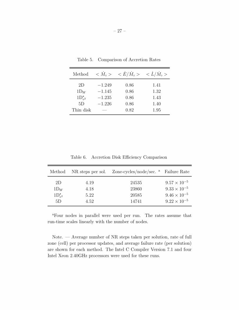
We have run this torus problem using the 2D, 1DW , 1D?v2 , and 5D inversion schemes.

The parameters are the same as before: {TOL, NNR, Nextra} = {10−10, 30, 2}. The resolution

is 2562. The initial conditions in each run also contain identical low level noise to initiate the

growth of the magnetorotational instability. The accretion rates of rest-mass, energy, and

angular momentum for these runs are shown in Figure 5. One would expect that after the

disk becomes turbulent (at ∼ 500 GM/c3 in this model) small differences in the solution due

to the inversion routines would be amplified and that the accretion rates would not track

each other very well. Evidently the accretion rates are nearly identical until 900 GM/c3,

after which their rates follow only vaguely similar trends. This suggests that the differences

in evolution due to the inversion routines were small indeed.

The average normalized accretion rates for the internal energy (E/M◦), angular mo-

mentum (L/M◦) and rest-mass (M◦) given in Table 5 differ by only a few percent. Far larger

– 20 –

differences were obtained by changing the seed used to generate the noise in the initial con-

ditions. In addition, the qualitative structure of the disks in steady-state remains the same

at the end of the evolutions. Shown in Figure 6 are snapshots of log(ρ◦) at t = 2000 GM/c3

from the runs using the 2D, 1DW , 1D?v2 and 5D methods (shown left to right, respectively).

The most pronounced differences are in the corona and funnel regions overlying the bulk of

the disk. Evidently the solution is stable to changes in the inversion algorithm.

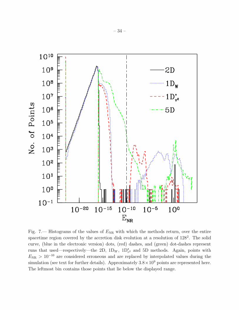
We have also compared low resolution (1282) runs using the four methods. This is

interesting because P exhibits larger fractional changes per timestep at lower resolution, so

the inversion routines are put under greater stress. In Figure 7, we show the distribution

of ENR exit values over the course of these simulations. The most striking feature of the

plot is in the number of points at which the 5D method fails to converge compared to other

methods. The 2D method rarely fails to converge, and the 1DW and 1D?v2 methods fail

to converge at nearly equal, intermediate rates. In Table 6 we state the failure rate—i.e.

the frequency at which either an unphysical P value is found or no solution is found—for

each 2562 run. The table demonstrates that the failure rates are approximately the same,

suggesting that when the 2D method “fails” it is converging to an unphysical P solution

instead of failing to converge altogether like the 5D method.

The inversion schemes are also faster in the disk evolution than in the parameter space

survey. This is seen in the distribution of NNR over the lower-resolution run shown in

Figure 8. Many more inversions in the disk run converge sooner than in the parameter space

survey. The greater efficiency and accuracy seen in the disk evolution is likely due to the

fact that in the disk evolution the inversion routine is usually supplied with better initial

guesses, from the previous timestep, than in the parameter space survey.

What is the optimal value of the Newton-Raphson parameters, {TOL, NNR, Nextra}, for

the most successful 2D and 1DW methods? Almost no new acceptable solutions are found

if we increase NNR > 30, so this is the natural value for this parameter. We also reran the

disk evolution using TOL = {10−3, 10−5, 10−7, 10−9, 10−10, 10−11} at a resolution of 2562.

Each run was otherwise identical and each used {NNR, Nextra} = {30, 2}. Surprisingly, we

discovered that the evolutions deviated little from each other until after the inner parts of

the disks become turbulent, at t ' 500M . The relative difference of any given primitive

function between any run and the TOL = 10−10 run grows as ∼ t7 until it plateaus to a

constant value at t & 1000M . Further, the accretion rates—i.e. those functions displayed

in Figure 5—were qualitatively indistinguishable until t ' 800M . The total number of NR

iterations executed during the course of a simulation also varied little between these runs.

Similar runs were made for TOL = {10−3, 10−9, 10−10, 10−11}, but now we reduced the

resolution to 1282. Since the timestep is larger in the lower resolution runs, guesses for

– 21 –

the primitive variables are—on average—further away from their solutions than in the 2562

resolution runs. As a result, the accretion rates and distribution of ENR differed dramatically

between the TOL = 10−3 run and the others. Runs with 10−11 < TOL < 10−9 have similar

accretion rates, and distributions of ENR and NNR. This implies that the guesses in the higher

resolution run are so close to their solutions that performing 3 iterations—the minimum

number of iterations allowed in the NR schemes when Nextra = 2—often leads directly to an

accurate solution independent of TOL.

These tests suggest that the tolerance, if below at least 10−3, is inconsequential to our

accretion disk simulations when the grid resolution is sufficiently high and when Nextra = 2.

To evaluate the sensitivity of the outcome to Nextra, we ran two 1282 disk models with

TOL = 10−6: one with no extra iterations and the other with Nextra = 2. The quantities

L/M◦, E/M◦, and M◦ deviate between the two runs by less 4% at any given time, far less

than what is seen between two otherwise identical runs at resolutions of 1282 and 2562. We

conclude that the inversion error is in some mean sense much less than the discretization

error when TOL is below 10−6.

The ENR distribution of the Nextra = 0 run is, however, significantly different than the

one shown in Figure 7. Without the extra iterations, the ENR distribution is approximately

uniform over 10−15 < ENR < 10−6, and becomes more similar to the NNR = 2 distribution for

ENR < 10−6. The extra iterations therefore seem to be doing what we expected for the most

part. In addition, using two extra iterations per inversion only increases the simulation’s run-

time by 4%. Even though this doubles the run-time contribution from the primitive variable

solver, it is still an insignificant portion of the evolution’s total computational cost, which

seems worthwhile to nearly eliminate the possibility that inversion error makes a significant

contribution to the computational error budget.

This investigation highlights the importance of handling aberrant cells in real applica-

tions. When an inversion fails to converge to a solution, when a solution leads to unphysical

primitive variables, or when it converges to a set of primitive variables which we have some

a priori reason for classifying as numerical artifacts, one must either halt the run or else

“correct” these values6. For example, the most common problem involves evolving to a state

of negative internal energy density. We have found that using an artificial floor can lead to

the generation of spontaneous “explosions.” These explosions can corrupt and eventually

terminate the evolution. We have found that 2nd-order interpolation of P from the prob-

lematic cell’s nearest-neighbors is successful at eliminating these cell-scale artifacts. This

interpolation procedure is used whenever at least one of the above conditions is met. All

6In accretion disk simulations we typically classify a point as aberrant if ρ◦, u ≤ 0, γ > 50, or γ < 1.

– 22 –

disk evolutions mentioned in this paper used this method.

6. Conclusion

We have outlined a compact derivation of the equations for calculating P(U). This

formulation suggests a variety of possibilities for performing the calculation numerically. We

have implemented a small subset of the possible methods, and compared these implemen-

tations through (1) a survey over a large subset of possible U values; (2) embedding the

inverter in a SRMHD code and evolving a cylindrical explosion problem due to Komissarov;

(3) embedding the inverter in a GRMHD code and evolving a turbulent, magnetized disk

around a rotating black hole.

Several key points emerge from the comparison. First, the implementation can be made

accurate enough that variable inversion does not make a significant contribution to the code

error budget. Second, some implementations can be made fast enough that they occupy only

a few percent of the total cycles used by our GRMHD code. Since we are using a particularly

simple GRMHD algorithm, this is likely an upper limit to the fractional cost of the inversion

in all GRMHD schemes. Third, the inversion routine originally used in HARM (Gammie,

McKinney, & Toth 2003), called “5D” here, is particularly slow and inaccurate.

We recommend the “2D” scheme, described in §3.2. A version of this scheme is available

for download on the web at http://rainman.astro.uiuc.edu/codelib/codes/pvs.tgz

This work was supported by NSF grants PHY 02-05155, AST 00-93091 and PHY99-

07949 (Kavli Institute for Theoretical Physics, where a portion of this work was completed).

We thank Yuk Tung Liu, Po Kin Leung and Xiaoyue Guan for comments.

REFERENCES

Anton, L., Zanotti, O., Miralles, J. A., Martı, J. Ma, Ibanez, J. Ma, Font, J. A. & Pons,

J. A., 2005, preprint (astro-ph/0506063)

Balbus, S. A. & Hawley, J. F. 1991, ApJ, 376, 214

Berger, M. J. & Oliger, J. 1984, J. Comp. Phys., 53, 484

Choptuik, M. .W. 1995, unpublished, http://bh0.physics.ubc.ca/People/matt/Doc/shadow0.ps

De Villiers, J. & Hawley, J. F. 2003, ApJ, 589, 458

– 23 –

Del Zanna, L., Bucciantini, N., & Londrillo, P. 2003, A&A, 400, 397

Duez, M. D., Liu, Y. T., Shapiro, S. L., & Stephens, B. C., 2005, preprint (astro-ph/0503420)

Eulderink, F., Mellema, G. 1995, A&AS, 110, 587

Fishbone, L. G. & Moncrief, V. 1976, ApJ, 207, 962

Fragile, P. C., 2005, preprint (astro-ph/0503305)

Gammie, C. F., McKinney, J. C., & Toth, G. 2003, ApJ, 589, 444

Gammie, C. F., Shapiro, S. L., & McKinney, J. C. 2004, ApJ, 602, 312

Harten, A., Lax, P. D. & van Leer, B. 1983, SIAM Rev., 25, 35

Koide, S., Nishikawa, K. -I., & Mutel, R. L. 1996, ApJ, 463, L71

Koide, S., Shibata, K., & Kudoh, T. 1999, ApJ, 522, 727

Komissarov, S. S. 1999, MNRAS, 303, 343

Komissarov, S. S. 2005, MNRAS, 359, 801

McKinney, J. C., Gammie, C. F. 2004, ApJ, 611, 977

Misner, C. J., Thorne, K., & Wheeler, J. A., Gravitation (W.H. Freeman and Co., San

Francisco, 1970)

Press, W. H., Teukolsky, S. A., Vetterling, W. T., & Flannery, B. P., Numerical Recipes in

C: The Art of Scientific Computing, (Cambridge University Press, Cambridge, 1992).

Rade, L. & Westergren, B., Beta Mathematics Handbook, (CRC Press, Boca Raton, 1990)

Weisstein, E. W., ”Cubic Equation,” from MathWorld–A Wolfram Web Resource,

http://mathworld.wolfram.com/CubicEquation.html

This preprint was prepared with the AAS LATEX macros v5.2.

– 24 –

Table 1. Physical Solutions for W of the 1Dv2 Scheme’s Cubic

Case Condition D W a

1 d32 > d0 > 0 D < 0 (40)

2 d32 < d0 > 0 , d2 6= 0 D > 0 (38)

3 d2 = 0 , d0 > 0 D > 0 W = (4d0)1/3

4 d32 = d0 > 0 D = 0 W = d2

5 d0 = 0 , d2 6= 0 D = 0 W = −3d2 iff d2 < 0

6 d2 = d0 = 0 D = 0 (none)b

aOnly physically-acceptable solutions, i.e. those that are real

and positive, are given here.

bThe only solution, W = 0, is unphysical.

– 25 –

Table 2. Kerr-Schild Coordinates (a = 0.9375) used in the Parameter Space Survey

cos(Φ)a r θ

-0.751 8.195 1.552

-0.250 1.375 1.444

-0.500 2.676 1.016

1.000 23.166 2.672

-0.997 26.467 0.658

0.500 1.571 1.589

0.749 3.588 1.455

0.250 2.406 2.483

-0.0005 35.480 0.146

Note. — Please refer

to the electronic version

of the Journal for a com-

plete, machine-readable

table of the parameters

used for the survey. The

larger table provides

x(1), x(2), r, θ, ui, Bj, gµν

for each value of cos Φ.

Please refer to Section 5.3

for a definition of the

coordinates.

acos(Φ) = uiBi√uiuiBjBj

– 26 –

Table 3. Parameter Space Efficiency Comparison

Method NR steps per sol. Sol. per sec. Failure Rate

2D 8.45 1.66 × 105 8.7 × 10−7

1DW 7.45 1.68 × 105 8.8 × 10−4

1D?v2 7.08 1.06 × 105 3.6 × 10−4

1Dv2 7.05 1.24 × 105 2.0 × 10−2

5D 19.3 1.89 × 104 4.2 × 10−1

Poly — 9.21 × 103 4.1 × 10−2

Note. — Average number of NR steps taken per solution,

average solution rate, and average failure rate (per solution)

are shown for each method. The first entry for the polyno-

mial method is vacant since it does not use the NR scheme.

The Intel C Compiler Version 8 and an Intel Xeon 3.06GHz

workstation were used for these runs.

Table 4. Cylindrical Explosion Efficiency Comparison

Method NR steps per sol. Zone-cycles/sec. Failure Rate

2D 3.81 74142 3.75 × 10−7

1DW 3.76 68966 3.75 × 10−7

1D?v2 4.68 58042 3.75 × 10−7

5D 4.45 27100 3.75 × 10−7

Note. — Average number of NR steps taken per solution, rate

of full zone (cell) updates, and average failure rate (per solution)

are shown for each method. The Intel C Compiler Version 8 and

an Intel Xeon 3.06GHz workstation were used for these runs.

– 27 –

Table 5. Comparison of Accretion Rates

Method < M◦ > < E/M◦ > < L/M◦ >

2D −1.249 0.86 1.41

1DW −1.145 0.86 1.32

1D?v2 −1.235 0.86 1.43

5D −1.226 0.86 1.40

Thin disk — 0.82 1.95

Table 6. Accretion Disk Efficiency Comparison

Method NR steps per sol. Zone-cycles/node/sec. a Failure Rate

2D 4.19 24535 9.57 × 10−5

1DW 4.18 23860 9.33 × 10−5

1D?v2 5.22 20585 9.46 × 10−5

5D 4.52 14741 9.22 × 10−5

aFour nodes in parallel were used per run. The rates assume that

run-time scales linearly with the number of nodes.

Note. — Average number of NR steps taken per solution, rate of full

zone (cell) per processor updates, and average failure rate (per solution)

are shown for each method. The Intel C Compiler Version 7.1 and four

Intel Xeon 2.40GHz processors were used for these runs.

– 28 –

Fig. 1.— Shown are the relative errors in calculating u from our parameter space survey

averaged over {ρ◦, B2, γ, Φ} and plotted versus log10(u). Only those points for which all

methods found a solution were included in the average, accounting for approximately 58%

of the surveyed points. The curves corresponding to the 2D, 1DW , 1D?v2 , 1Dv2 , 5D, and

polynomial methods are represented by, respectively, circles, (blue in the electronic edition)

exes, (red) squares, (magenta) asterisks, (green) empty triangles, and (cyan) filled triangles;

please note that the 2D, 1DW , 1D?v2 , and 5D relative errors are almost indistinguishable. See

the electronic edition of the Journal for a color version of this figure.

– 29 –

Fig. 2.— Histograms of the final value of ENR per parameter space point for the methods

using a NR scheme. The distributions generated from the 2D, 1DW , 1D?v2 , 1Dv2 and 5D

methods are represented, respectively, by a solid line, (blue in the electronic edition) dots,

(red) dashes, (magenta) long dashes, and (green) dot-dashes. Only those parameter space

points for which all methods converged to a solution were included in this figure, so all points

lie below ENR = 10−10. There are approximately 3.3 × 106 points per histogram. The first

bin contains those points that lie beneath the displayed range. See the electronic edition of

the Journal for a color version of this figure.

– 30 –

Fig. 3.— Histograms of the number of NR iterations taken by the methods per parameter

space point. The distributions generated from the 2D, 1DW , 1D?v2 , 1Dv2 and 5D methods are

represented, respectively, by a solid line, (blue in the electronic edition) dots, (red) dashes,

(magenta) long dashes, and (green) dot-dashes. Only those parameter space points for which

all methods converged to a solution were included in this figure. There are approximately

3.3 × 106 points per histogram. See the electronic edition of the Journal for a color version

of this figure.

– 31 –

Fig. 4.— Snapshots of Bx (top left), By (top right), log10 p (bottom left) and γ (bottom

right) taken at t = 4 from the cylindrical explosion evolution. A continuous greyscale from

white to black is used for each plot, using the same limits as used by Komissarov (1999):

Bx ∈ [0.008, 0.35], By ∈ [−0.18, 0.18], log10 p ∈ [−4.5,−1.5], γ ∈ [1, 4.57]. The lower-right

plot also shows the magnetic field lines that originate from x = −6 and along the y-axis at

equal intervals of dy = 1/3 from −5.67 to 5.67.

– 32 –

Fig. 5.— Accretion rates of rest-mass, specific energy and specific angular momentum over

time for a disk evolution around a Kerr black hole of spin parameter a = 0.9375M at

a resolution of 2562. The solid curve, (blue in the electronic version) dots, (red) dashes,

and (green) dot-dashes represent runs that used—respectively—the 2D, 1DW , 1D?v2 and 5D

methods. All the straight horizontal lines indicate the time-averages of the accretion rates

over t = 500− 2000 GM/c3 for the different methods except for the (cyan) lines of dots and

long dashes which denote the thin disk values. See the electronic edition of the Journal for

a color version of this figure.

– 33 –

Fig. 6.— Snapshots of log ρ◦ at t = 800 GM/c3 (top row) and t = 2000 GM/c3 (bottom row)

on a 2562 grid are shown from accretion disk evolutions using different methods: (from left

to right) the 2D, 1DW , 1D?v2 and 5D methods. The data are plotted here in (r, θ) coordinates

in the xy-plane. The region we exclude about the origin to excise the singularity from the

grid can be seen near the origin. The color map is logarithmically-spaced such that the black

(dark blue in the electronic version) points refer to ρ◦ ' 4× 10−7, while the white (dark red

in the electronic version) regions correspond to ρ◦ ' 0.69. See the electronic edition of the

Journal for a color version of this figure.

– 34 –

Fig. 7.— Histograms of the values of ENR with which the methods return, over the entire

spacetime region covered by the accretion disk evolution at a resolution of 1282. The solid

curve, (blue in the electronic version) dots, (red) dashes, and (green) dot-dashes represent

runs that used—respectively—the 2D, 1DW , 1D?v2 and 5D methods. Again, points with

ENR > 10−10 are considered erroneous and are replaced by interpolated values during the

simulation (see text for further details). Approximately 3.8×109 points are represented here.

The leftmost bin contains those points that lie below the displayed range.

– 35 –

Fig. 8.— Histograms of the number of NR iterations taken by the methods over the entire

spacetime region covered in the accretion disk evolution at a resolution of 1282. Approxi-

mately 3.8×109 points are represented here. The bin located at NNR = 31 contains all those

points for which no solution was found, all other points were successful.