primus: pedigree reconstruction and identification of a maximum
TRANSCRIPT

PRIMUS: Pedigree Reconstruction and Identification of a Maximum Unrelated Set
Jeffrey Staples
A dissertation
submitted in partial fulfillment of the
requirements for the degree of
Doctor of Philosophy
University of Washington
2014
Reading committee:
Deborah Nickerson
William Noble
Bruce Weir
Program Authorized to Offer Degree:
Genome Sciences

v
©Copyright 2014 Jeffrey Staples
vi
University of Washington
Abstract
PRIMUS: Pedigree Reconstruction and Identification of a Maximum Unrelated Set
Jeffrey Staples
Chair of the Supervisory Committee:
Professor Deborah A. Nickerson
Department of Genome Sciences
This dissertation describes the methods and algorithms developed to improve human
genetic analysis for both genome-wide association studies (GWAS) and pedigree-based
analyses. The new algorithms are included in the software package PRIMUS. There are
four main parts of PRIMUS:
1) To identify a maximum unrelated set of individuals within a genetic dataset to
improve statistical analyses.
2) To reconstruct pedigrees using genome-wide identity by descent estimates.
3) To improve pedigree reconstruction using mitochondrial and non-recombining Y
haplotypes.
4) To extend pedigree reconstruction by PRIMUS beyond third degree relationships
using distant pairwise relationship predictions.
vii
Table of Contents
List of Figures ix List of Tables xi Acknowledgements v Chapter 1 Introduction and background 1 Chapter 2. Identification of a maximum unrelated set 5 Introduction 5 Methods 5 Current approaches 5 New Method 7 Weighted Maximum Set Selection 9 The Approximation Function 10 Family Network Simulations 10
Results 12 Simulation Results 13 HapMap3 Results 13
Discussion 21 Chapter 3. PRIMUS: Rapid reconstruction of pedigrees from genome-‐wide estimates of identity by descent 23 Introduction 23 Methods 26 Simulated pedigrees 26 IBD estimates 31 Family network identification 31 Familial relationship prediction using a kernel density estimation (KDE) function 31 Pedigree reconstruction algorithm 37 Automatically adjusting likelihood threshold 38 Pedigree scoring 38 PRIMUS results and output 39 Pedigree checking program 39 Reconstructing authentic pedigrees 39 Exome sequence data and corresponding pedigrees 40
Results 40 Confirming and correcting clinically ascertained pedigrees 45
viii
Reconstructing and incorporating cryptic relatedness 49 Reconstruction of previously unknown pedigrees from Starr County 52 Comparing PRIMUS to competing methods 52
Discussion 55 Chapter 4. Incorporating mtDNA and NRY haplotypes into pedigree reconstruction 62 Introduction 62 Methods 63 Identifying concordant and discordant mtDNA and NRY haplotypes 63 mtDNA and NRY checking 64
Results 64 Chapter 5. PADRE: Pedigree Aware Distant Relationship Prediction 72 Introduction 72 Methods 73 Pedigree Aware Distant Relationship Estimation (PADRE) algorithm 73 Controlling for Type 1 error 75 Simulations 76 Extended Pedigree Samples 77 HapMap3 CEU samples 77 Pedigree reconstruction with PRIMUS 77 Distant relationships prediction with ERSA 77
Results 78 Simulations 78 Extended pedigree results 79 Results for HapMap3 CEU samples 79
Discussion 85 Chapter 6. Summary and future directions 88 Significant Contributions 88 Future Directions 89 Complex relationships 89 Consanguineous relationships 89 Distant relationships 90
Conclusion 91 References 93 Supplementary Tables 99

ix
List of Figures Figure 1. Stepwise selection process of an unrelated set for the three alternative methods and
PRIMUS. ........................................................................................................................................................... 7 Figure 2. Example of a family network graph. .............................................................................................. 8 Figure 3. PRIMUS run-‐times on the simulations. ...................................................................................... 11 Figure 4. The diversity of sizes and connectivity levels for family networks in real data. ........ 12 Figure 5. A heatmap showing the percent increase in unrelated sample size by PRIMUS
compared to PLINK's suggested method. .......................................................................................... 14 Figure 6. Heatmaps comparing PRIMUS and three other methods on simulated data. .............. 16 Figure 7. Heatmaps comparing PRIMUS and three other approaches to identify unrelated sets
on simulation data when using the binary weighting functions. .............................................. 19 Figure 8. Schematic of a simulated 12-‐person pedigree. ....................................................................... 28 Figure 9. Examples of simulated pedigrees of size 20. ........................................................................... 29 Figure 10. Comparison of the true IBD1 value to the PLINK IBD1 estimates for relationship
sampled from 1000 size-‐12 pedigrees. .............................................................................................. 30 Figure 11. False positive (FP) and false negative (FN) relationship predictions with different
KDE bandwidths and likelihood cutoffs for full-‐sibling (FS), 2nd degree, 3rd degree, distant (DIS) and unrelated (UN) relationships. ........................................................................................... 35
Figure 12. Kernel density distributions of the trained kernel density estimates for each familial relationship category. ............................................................................................................. 36
Figure 13 (Figure 1). A summary of the reconstructions for a thousand simulated pedigrees by PRIMUS. ........................................................................................................................................................ 42
Figure 14. Results from the reconstruction of simulated pedigrees. ................................................ 43 Figure 15. Simulation runtime results. ........................................................................................................ 46 Figure 16. A pedigree correctly reconstructed by PRIMUS in nine seconds. .................................. 47 Figure 17. Two EOCOPD pedigrees verified by PRIMUS. ........................................................................ 47 Figure 18. Two of the six EOCOPD pedigrees corrected by PRIMUS. .................................................. 48 Figure 19. A ten-‐person MapMap3 MXL pedigree obtained from the HapMap3 and 1000
Genomes samples. ..................................................................................................................................... 51 Figure 20. Comparison of relationship prediction accuracies for simulated pedigrees using
RELPAIR and PRIMUS. ............................................................................................................................. 54 Figure 21. Examples of simple and common pedigrees structures. ................................................... 55 Figure 22. A pedigree from the University of Washington Center for Mendelian Genomics. ... 59 Figure 23. An example where pairwise relationship checking and removal of an inconsistent
sample results in an analysis loss. ....................................................................................................... 60 Figure 24. An example where pairwise relationship checking and removal of an inconsistent
samples results in an unnecessary data loss and the use of an incorrect pedigree. .......... 61 Figure 25. Summary of the haplotype discordance between pairs of individuals. ....................... 66 Figure 26. Examples of (A) mtDNA and (B) NRY inheritance paths in a pedigree. ........................ 67

x
Figure 27. A summary of the percent reduction in the average number of possible pedigrees when data from mtDNA haplotypes, NRY halpotypes, sex or all of these are applied in pedigree analysis. ..................................................................................................................................... 68
Figure 28. Relative improvement of reconstruction of simulated pedigrees with 35% masked samples with additional data (i.e., sex status, NRY and mtDNA haplotypes). ...................... 69
Figure 29. A reconstructed simulated pedigree uniquely identified with mtDNA data. ............. 70 Figure 30. This pedigree structure was used to simulate ninth-‐degree pedigrees. ..................... 78 Figure 31. ERSA and PADRE performance on simulations. ................................................................... 81 Figure 32. PADRE and ERSA results on complete simulated pedigrees. ........................................... 82 Figure 33. Percentage of correct relationship estimations by PADRE on extended European
ancestry pedigrees compared to the simulated pedigree results. ........................................... 83 Figure 34. A graph of PADRE estimated relationships among the CEU samples using a
Bonferroni correction of p = 5.5x10-‐6 for pairwise relationships between network founders. ...................................................................................................................................................... 84
Figure 35. An example of four distantly related HapMap3 CEU pedigrees with relationships predicted by PADRE. ................................................................................................................................ 85
xi
List of Tables Table 1. Minimum network size for which the approximation function of PRIMUS is applied. 12 Table 2. The number of simulations where other methods outperform the approximation
function in PRIMUS. .................................................................................................................................. 17 Table 3. Comparison of PRIMUS and other methods on publicly available datasets. .................. 20 Table 4. Expected mean IBD proportions for the outbred familial relationship categories ..... 28 Table 5. A summary of the concordance between pairs of individuals known to have
concordant mtDNA or NRY haplotypes. ............................................................................................. 71 Supplementary Table 1. True IBD vs. Estimated IBD for different SNP sets ................................... 99 Supplementary Table 2. Combined simulation reconstruction results .......................................... 100 Supplementary Table 3. The accuracy of PRIMUS and RELPAIR relationship predictions with
Halfsib size-‐20 pedigrees ..................................................................................................................... 101 Supplementary Table 4. EOCOPD pedigree reconstruction summary ............................................ 103 Supplementary Table 5. Comparison of HapMap3 pairwise relationships ................................... 106 Supplementary Table 6. Possible combinations of pairwise 2nd and 3rd degree family
relationships considered during pedigree reconstruction ...................................................... 125

v
Acknowledgements
I would like to thank my advisor, Debbie Nickerson, for her support throughout my
project. She provided me the opportunity and flexibility to work on the topics and
projects that interested me. Working with Debbie has provided me with access to the best
data on the planet and the opportunity to present my work in a variety of settings to broad
audiences. It has been an honor to have her as my mentor. I greatly appreciated her
guidance on my research, presentations, networking, and job negotiations.
I would also like to thank Piper Below for her collaboration and friendship through much
of my time at University of Washington. We made a great team bouncing ideas off one
another and working together to find solutions to the problems we encountered. She was
there to give me advice and help when needed which was extremely valuable.
I am grateful for my fellow Nickersonians and everyone in Genomes Sciences and
beyond. In particular, Adam Gordon for our countless discussions on research, plots, and
science; Colleen Davis for improving everyone of my papers, posters, and talks; Chad
Huff for his patience and willingness to help with PADRE in a short time frame; Bruce
Weir, Phil Green, Bill Noble, Brian Browning, Larry Ruzzo, Ellen Wijsman, Elizabeth
Thompson, Peggy Robertson, Qian Yi, Guillaume Jumenez, Tom Kolar, and Christa Poel
for so many helpful discussions and assistance; and the Genome Training Grant and the
National Science Foundation for funding my work.
Finally and most importantly, I want to thank my family for their support. My wife,
Katie, and my children, Landon and Moira, have given me their unconditional love,
support, and patience throughout my graduate studies UW. I thank my parents for their
encouragement and advice. I also thank my siblings and other family members for their
interest and support.
1
Chapter 1 Introduction and background
The relationship of genotype to phenotype is central to genetic analysis. Differences in DNA can
alter phenotypic expression for simple traits (e.g., those influence by a single gene such as the
ability to digest lactose) to more complex traits (e.g., that are modified by variation in thousand
of loci such as height)1. A small fraction of the changes in DNA result in the expression of
abnormal phenotypes and diseases1. If identified, these disease-causing DNA variants can
provide key insights into human biology and can point to treatments or cures for a disease2. To
this end, geneticists have tracked the inheritance of disease-causing variants through families and
pedigrees3. Geneticists use pedigrees and powerful tools like linkage analysis to identify the
region(s) in the genome that contains the variant with functional impact. If the pedigree is large
with many informative meioses, then it is possible to identify the gene that contains the disease-
causing variant with the analysis of the single family and appropriate biological studies.
Today, pedigrees continue to be utilized to determine the heritability and genetic models for
traits and disorders4-6. Knowing the exact pedigree structure allows investigators to correctly
identify the mode of inheritance for a disorder. These approaches utilize powerful statistical
tools that require, or benefit from, the correct pedigree structure such as: linkage7, family-based
association8, pedigree-aware imputation, pedigree-aware phasing, Mendelian error-checking,
and, heritability. Furthermore, in many instances, knowing that the pedigree is consistent with
the genetic data is crucial to identifying the association variants and genes linked to a disease or
disorder4-6; 9.
The development of large-scale genotyping has brought genome-wide association studies
(GWAS) to the forefront. This type of study compares the genotypes of a group of individuals
with a disease (cases) to a group of similar people without the disease (controls) or looks at a
phenotypic trait. From 2005-2013, the GWAS catalog at http://www.genome.gov/gwastudies/
reported thousands of GWAS have identified more than 14,000 single-nucleotide polymorphisms
associated with phenotypic traits10. GWAS analysis requires care to not violate the assumption of
independence of samples. For instance, interrelatedness can inflate the false positive rate in a
GWAS11; 12, resulting in spurious associations. Interrelatedness can also introduces biases in
many statistical analyses, including an inflated false positive rate in burden tests, over-estimation
2
of relatedness in genome-wide estimates of identity by descent (IBD)13, and skewed principle
component analyses14. Interrelatedness must be removed before performing these analyses.
I have developed several new computational tools to improve both the removal of interrelated
samples and to identify pedigrees in genetic datasets that can also be used for analyses. First, I
address the issue of removing interrelatedness within datasets. Unless modeled in the statistical
analysis15; 16, related samples must be removed prior to genetic analyses to limit potential biases.
Given the expense of sample ascertainment, phenotyping as well as the genotyping and/or
sequencing, maximizing the number of unrelated samples in any dataset should be a priority.
However, available methods and suggestions for removal of related samples do not guarantee the
retention of the maximum number of unrelated samples in a dataset. To improve on existing
approaches, individuals in a dataset are visualized as nodes in a graph and relationships between
individuals as edges between the nodes. Graph theory algorithm developed by Bron and
Kerbosch17 is then applied to identify the maximum unrelated set of individuals from any genetic
dataset. I have implement this adapted algorithm in a software package known as Pedigree
Reconstruction and Identification of the Maximally Unrelated Set or PRIMUS18.
Second, I set out to improve approaches to reconstruct pedigrees. Pedigree analysis, through
linkage studies, has become a mainstay in human genetics, and the underpinnings of more than
3,500 Mendelian diseases and disorders have been identified (references including OMIM).
Significant effort is spent collecting and maintaining accurate sample records for pedigrees.
However, despite the best efforts of investigators, pedigree and sample errors are still quite
common and require careful examination to avoid a reduction in power to detect linkage19. The
rate of non-paternities in studies has been reported between 0.8% and 30% (median 3.7%;
n=17)20, with other reports showing more conservative estimates of 1% to 1.5%21; 22. Even at the
conservative rate of 1%, a pedigree with six children has a 6% chance of being incorrect due to a
non-paternity, and the pedigree error rate will be much higher after accounting for other common
errors such as sample swaps, duplicate samples, contamination, and other relationship
discrepancies.
The standard practice for checking and correcting pedigrees and relationships within genetic
datasets is to use pairwise prediction programs23-27 like RELPAIR28 and PREST29 to verify that

3
the level of relatedness between every pair of individuals falls close to the expected level of
relatedness based on the reported pedigree30-37. While using pairwise estimates to check
relationships in pedigrees is sometimes sufficient, there are four major drawbacks. First, pairwise
checking will not catch pedigree errors if there are multiple pedigree structures that fit the
genetic data. Second, pairwise relationship checking does not provide, or even suggest, the
correct pedigree in the case of inconsistency between the data and the reported pedigree. Third,
pairwise inconsistencies between genotyped samples are often resolved by removing the
inconsistent sample(s), which can result in the unnecessary loss of samples or in accepting an
incorrect pedigree as true. Finally, manually reconstructing an unknown pedigree manually using
pairwise relationship comparisons is arduous and error-prone.
A solution to these drawbacks is to use the genetic data to reconstruct the corresponding pedigree
structure. Pedigree reconstruction will identify inconsistencies between the reported pedigree,
and the genetic data will also provide the correct pedigree. Unfortunately, existing pedigree
reconstruction programs have a variety of limitations that prevent them from being broadly
applied to reconstructing and verifying human pedigrees. I have developed a pedigree
reconstruction method without many of the limitations of previous pedigree reconstruction
programs and have incorporated it into PRIMUS. This approach utilizes the power of single
nucleotide polymorphism (SNP) arrays or next-generation sequence data to evaluate genome-
wide estimates of IBD that are generated by programs such as PLINK23 or KING25. In order to
reduce the number of possible pedigrees and increase the chances of identifying the true pedigree
structure, I also extended the algorithm to use mitochondrial (mtDNA) and non-recombining Y
chromosome (NRY) haplotypes to reduce the number of pedigrees generated by PRIMUS and to
improve the chances of identifying the correct pedigree. This decreases runtime and improve the
overall reconstruction results.
Finally, I merged the power of PRIMUS with a program that is capable of reconstructing more
distant relationships. PRIMUS provides an accurate prediction of relationships up to third-degree
(e.g., first-cousins) and can provide complete pedigree structures for individuals in a genetic
dataset. However, there are often only clusters of close relationships within genetic datasets,
resulting in sparse pedigrees with many relationships more distant than third-degree
relationships. These sparse datasets are well suited for pairwise-prediction algorithms that can

4
accurately predict relationships up to ninth-degree relatives (third-cousins once removed).
However, these pairwise prediction programs are not capable of reconstructing close
relationships into complete pedigrees, and they are limited to accurate predictions of ninth-
degree relatives38. I developed and implemented an algorithm that leverages the pedigree
reconstruction of first- through third-degree relatives by PRIMUS with the accurate distant
relationship predictions by Estimation of Recent Shared Ancestry (ERSA)38. This algorithm is
known as PADRE, (Pedigree Aware Distant Relationship Estimation) and I have implemented it
in PRIMUS. The PADRE algorithm uses ERSA relationship likelihoods to calculate the most
likely connection between family networks reconstructed by PRIMUS. By combing the power of
pedigree reconstruction with PADRE, we can now connect distantly related pedigrees that can be
used for a more powerful linkage analysis.

5
Chapter 2. Identification of Maximum Unrelated Set
Introduction
Interrelatedness can be a confounding factor in many statistical analyses, including burden tests
in sequence data, association studies11; 12, genome-wide estimates of IBD13, and principle
component analyses14. Unless modeled in the statistical analysis15; 16, interrelatedness must be
removed from the data before proceeding with genetic analyses. Given the expense of DNA
ascertainment, clinical phenotyping, sequencing and/or genotyping, and data analysis,
maximizing the number of unrelated samples utilized in such analyses should be a priority.
Estimates of pairwise IBD, a quantitative measure of relatedness, can reliably detect relatives as
distant as first cousins39. Over the years, multiple strategies to detect IBD have been developed23;
25; 39-43, and new methods are emerging that use IBD estimates to confidently detect more distant
relatives (up to third-cousins)39; 40. With good IBD estimates, relatedness structures that violate
the assumption of sample independence can be identified and removed from the dataset through
sample pruning.
Methods
Current approaches
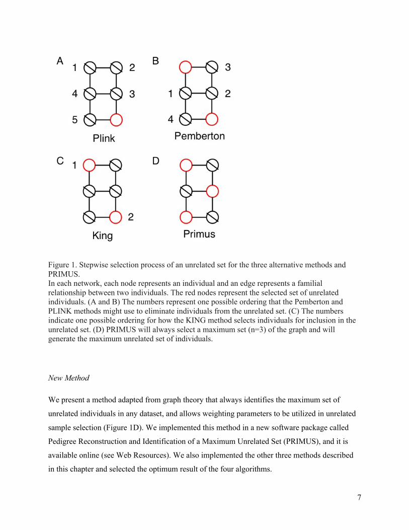
We have identified three publicly available methods to produce a set of unrelated individuals
given a threshold of tolerated pairwise IBD. The documentation for PLINK23 (see Web
Resources) suggests a method to remove pairwise relatedness by iteratively removing one
member of each pair until no pairs remain (Figure 1A). Pemberton et al.44 suggest generating
networks of relatedness in which samples are nodes and pairwise relationships are edges.
Relatedness networks are then broken by iteratively removing the most highly connected node,
until no edges remain in the dataset (Figure 1B). Finally, the authors of KING25 describes how
they generate a set of unrelated individuals in a recent paper45. They first add the person who is
related to the fewest other people in the dataset and then proceed to add the individual who is
related to the next fewest people in the dataset, as long as the individual to be added is not related
to anyone already in the set of unrelated individuals (Figure 1C). However, none of these

6
approaches maximize the number of retained unrelated samples or selectively retain the most
informative samples, as I demonstrate in Figure 1. Solving this problem is proven to be hard
(algorithms to solve this problem run in exponential time46) and much graph theory has been
dedicated to solving it47.
I have chosen to utilize existing graph theory to solve this problem by formulating the family
networks as a graph, where individuals are represented as nodes and relationships between
individuals are edges. In graph theory, the maximum unrelated set is referred to as the maximum
independent set; the maximum independent set of a graph is the same as the maximum clique of
the complement graph. To obtain the complement of a graph, all missing edges are added, and all
existing edges of the graph are removed. Here, this is equivalent to forming edges when
relationships fall below the user-defined relatedness threshold rather than above it. We then
search this complement graph for a maximum clique. A clique is defined as a portion of the
graph (subgraph) where each node is connected to every other node in the subgraph. A maximal
clique is a clique that is not a subgraph of a larger clique. Finally, a maximum clique is the
largest maximal clique. The maximum clique of the complement graph of our relationships
networks is thus the maximum unrelated set.
In order to test PRIMUS and compare it to other methods, we programmed each of the three
methods as described (Figure 1). This was required because neither of the methods described in
PLINK or Pemberton are available in a software package, and the KING program does not allow
for the input of user-defined IBD estimates. Rather, KING calculates its own IBD estimates from
input genotype data.
7
Figure 1. Stepwise selection process of an unrelated set for the three alternative methods and PRIMUS. In each network, each node represents an individual and an edge represents a familial relationship between two individuals. The red nodes represent the selected set of unrelated individuals. (A and B) The numbers represent one possible ordering that the Pemberton and PLINK methods might use to eliminate individuals from the unrelated set. (C) The numbers indicate one possible ordering for how the KING method selects individuals for inclusion in the unrelated set. (D) PRIMUS will always select a maximum set (n=3) of the graph and will generate the maximum unrelated set of individuals.
New Method
We present a method adapted from graph theory that always identifies the maximum set of
unrelated individuals in any dataset, and allows weighting parameters to be utilized in unrelated
sample selection (Figure 1D). We implemented this method in a new software package called
Pedigree Reconstruction and Identification of a Maximum Unrelated Set (PRIMUS), and it is
available online (see Web Resources). We also implemented the other three methods described
in this chapter and selected the optimum result of the four algorithms.
8
PRIMUS reads in user-generated IBD estimates and outputs the maximum possible set of
unrelated individuals, given a user-defined threshold of relatedness. PRIMUS converts the IBD
relationship file to an undirected graph in which nodes represent individuals and edges represent
pairwise relationships; each connected component represents a “family network” or pedigree.
PRIMUS writes out each family network to a .dot file to be viewed in graph visualization
software like GraphViz (see Web Resources) to generate images of the family networks (see
Figure 2).
Figure 2. Example of a family network graph. Each node represents an individual in the family network and each edge shows a relationship between two individuals. A graph like this will be generated for each family network with more than two people.
All individuals within each family network of the data are unrelated to any individual in a
different family network (at the user-specified threshold). Thus, the problem of identifying the
maximally sized unrelated set is reduced to finding the maximum unrelated set within each
family network and then combining the unrelated sets of each family network to get the
maximum unrelated set of the entire graph/dataset.
9
PRIMUS uses the Bron-Kerbosch algorithm17 with improved pivot selection48 to enumerate all
maximal cliques of each complement family network. The Bron-Kerbosch algorithm using a
recursive backtracking algorithm to enumerate all maximal cliques and then selects the largest of
the maximal cliques. For each family network, PRIMUS picks the maximum clique or the
weighted maximum clique to add to the maximum unrelated set of individuals. Finally, it
generates a file containing the maximum set of unrelated individuals.
Weighted Maximum Set Selection
A unique strength of our program is its ability to weight the maximum clique selection using
additional criteria. The maximum clique is the clique containing the most samples; however,
there are often two or more maximum cliques. Any one of these will produce a maximum
unrelated set, and PRIMUS allows for preferential selection of the maximum clique based on
additional weighting criteria. In case/control studies this function is particularly useful, because it
allows for the retention of the maximum clique with the most affected individuals. Alternatively,
the user may wish to select the maximum clique with the lowest missingness rate within the data,
or perhaps to first select for affected status and then for lowest missingness. PRIMUS allows
specification of as many of these weighting criteria as desired as well as ordering how they are
applied in the selection. No other available method for selecting unrelated samples offers
weighting functionality.
PRIMUS can also retain the maximum number of unrelated individuals with a desired binary
characteristic (e.g. affected status), even if this unrelated set is smaller than the maximum set of
unrelated individuals. For example, a study may contain a trio with an affected child and two
unaffected parents. The maximum unrelated set would require removing the child and retaining
both parents, since the parents are unrelated to each other. It is likely one would wish to retain
the single affected child for further analysis instead of both unaffected parents. As a result, the
overall unrelated set size will be smaller, but the set will contain more of the affected samples.
Since none of the PLINK, Pemberton, and KING methods has a weighting algorithm, we
implemented one for each. These implementations are available upon request. For the PLINK
method, we implemented weighting by selecting the individual with the desired trait. For
example, to preferentially select affected individuals, the algorithm will keep the affected
10
individual in a case-control related pair. For the Pemberton method, we implemented a weighting
scheme by choosing to remove the node with the less optimal criteria whenever two nodes are
equally connected. For the KING method, we implemented weighting by retaining the more
desirable individual whenever two individuals are related to the same number of other
individuals.
The Approximation Function
The Bron-Kerbosch algorithm is impractical to run on large, sparse family networks due to the
algorithm’s exponentially increasing computational cost (Figure 3). To remedy this, we
implemented an approximation function for networks above a set cutoff size (Table 1).
PRIMUS’ approximation function takes a similar approach to the Pemberton method44 by
repeatedly removing the highest degree node from the family network until the network is
smaller than the approximation function size cutoff or until it breaks into sub-networks smaller
than the cutoff. Once the size of the network or sub-networks is below the approximation
function size cutoff, PRIMUS uses the Bron-Kerbosch algorithm to obtain an independent set
that is approximately the largest. We do acknowledge that we do not know how good this
approximation is and would benefit from additional testing.
Family Network Simulations
To compare the performance of PRIMUS to these methods on all types of family networks, we
randomly generated 7,500 simulated family networks of varying sizes and network connectivity,
which is a measure of how interconnected the network is. Connectivity is the number pairwise
relationships that exist in a dataset divided by the total possible number of pairwise relationships.
Connectivity can vary widely in family data (Figure 4); some family networks are highly
connected (e.g. a father, mother, and 10 offspring), while other family networks may be sparsely
connected (e.g. a ‘string’ of cousins in which each is related through a unique parent). For each
network size (5 to 130 by increments of five) we randomly generated 30 simulated networks
with the network connectivity proportion ranging from 0.1 (10% of all possible pairwise
relationships exist in the network) to 1 (every individual is related to every other individual), and
our simulation data is available upon request. For each simulation, we obtained an unrelated set
from PRIMUS and the three other methods.

11
Figure 3. PRIMUS run-times on the simulations. The dashed lines show the exponential run-time and computational infeasibility of the Bron-Kerbosch algorithm for large network sizes. The solid colored lines show the run-times of PRIMUS. The dashed and solid lines separate when as PRIMUS’ approximation function is used to avoid the exponential run-times
12
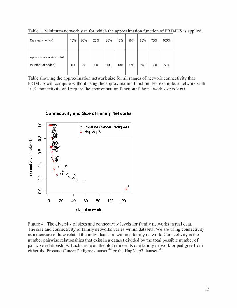
Table 1. Minimum network size for which the approximation function of PRIMUS is applied.
Connectivity (<=) 15% 20% 25% 35% 45% 55% 65% 75% 100%
Approximation size cutoff
(number of nodes) 60 70 90 100 130 170 230 330 500
Table showing the approximation network size for all ranges of network connectivity that PRIMUS will compute without using the approximation function. For example, a network with 10% connectivity will require the approximation function if the network size is > 60.
Figure 4. The diversity of sizes and connectivity levels for family networks in real data. The size and connectivity of family networks varies within datasets. We are using connectivity as a measure of how related the individuals are within a family network. Connectivity is the number pairwise relationships that exist in a dataset divided by the total possible number of pairwise relationships. Each circle on the plot represents one family network or pedigree from either the Prostate Cancer Pedigree dataset 49 or the HapMap3 dataset 50.
13
Results
Simulation Results
In all 6,540 simulations that did not require the use of the approximation function, PRIMUS
produced an unrelated set of size equal to or greater than all other approaches. In our simulations,
PRIMUS increased the unrelated set size by more than 50% relative to the PLINK method
(Figure 5) and by similar amounts relative to the other selection methods (Figure 6). Although
PRIMUS provides the greatest improvement as the network size and connectivity increase, even
for sparse, small networks PRIMUS typically provides 5-20% improvement compared to the
other methods (Figure 6).
Only when the PRIMUS’ approximation function was used (960 simulations) do the other
methods have the potential to outperform PRIMUS. The Pemberton method never outperforms
PRIMUS because PRIMUS’ approximation function is very similar to the Pemberton method
while the size of the network is above the approximation size thresholds shown in Table 1. Table
2 shows that PRIMUS’ approximation function outperforms the other three methods in more
than 98.75% of the simulations. To address the 1.25% of cases, we have incorporated each of the
other methods into PRIMUS, such that when it recognizes the need to run the approximation
function, it will also run each of the other methods and return the largest unrelated set derived
from any of the four methods.
We also compared the performance of each method on weighting for a binary and a quantitative
trait. Similar to the maximum unrelated set identification, PRIMUS always identifies the largest
set of unrelated affected individuals when the approximation function is not needed. PRIMUS
retained up to 75% more affected individuals in the weighted comparisons between PRIMUS
and each of the other methods (Figure 7).
HapMap3 Results
Finally, we compared the performance of PRIMUS and the other three methods on data from
Phase 3 of the Haplotype Mapping Project50 and the 1000 Genomes Project51. For each dataset,
PRIMUS obtained the largest set of unrelated individuals (see Table 3). Given our IBD estimates

14
for these reference datasets, the maximum sample set in which no pair of individuals have a
coefficient of relatedness ( ) > 0.1 are listed in Table 3 and a link to a list of the sample IDs can
be found at the PRIMUS website (see Web Resources).
Figure 5. A heatmap showing the percent increase in unrelated sample size by PRIMUS compared to PLINK’s suggested method. The vertical axis is the number of edges in the network divided by the total number of possible edges. The horizontal axis is the size of the simulated network. The color in each square corresponds to the percent increase in the size of the unrelated sample set generated by PRIMUS relative to the set generated by PLINK averaged across 30 randomly generated networks.
π̂
15
16
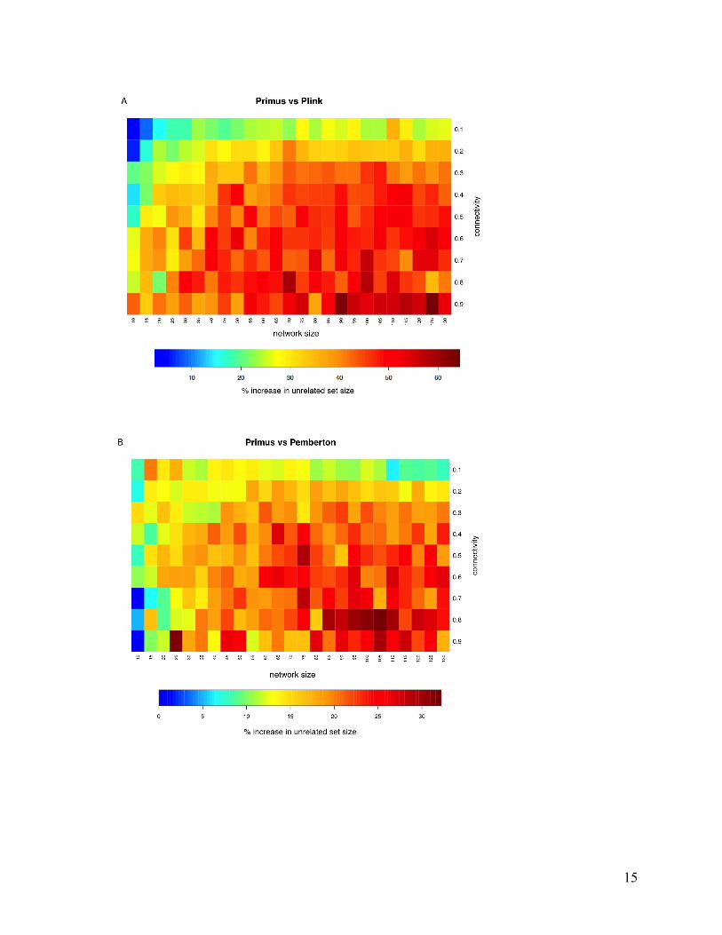
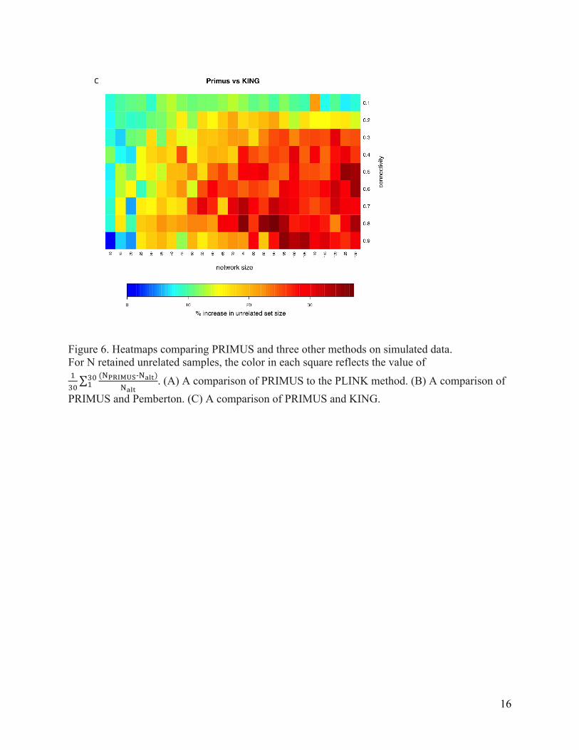
Figure 6. Heatmaps comparing PRIMUS and three other methods on simulated data. For N retained unrelated samples, the color in each square reflects the value of !!"
(!!"#$%&-‐!!"#)!!"#
!"! . (A) A comparison of PRIMUS to the PLINK method. (B) A comparison of
PRIMUS and Pemberton. (C) A comparison of PRIMUS and KING.

17
Table 2. The number of simulations where other methods outperform the approximation function in PRIMUS.
Weighting Criteria PLINK Pemberton KING % of total
No weighting 1/960 0/960 6/960 0.24%
Affected status 51/960 0/960 0/960 1.77%
Low quantitative trait 2/960 0/960 19/960 0.73%
There were 960 simulations that required PRIMUS to use its approximation function. The table shows out of those 960 simulations how many simulations did the other methods outperform PRIMUS.
18
19
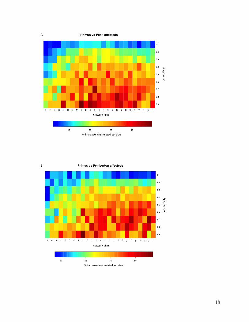
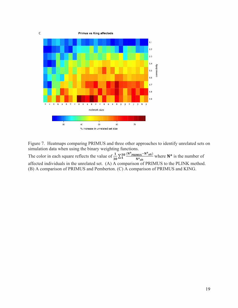
Figure 7. Heatmaps comparing PRIMUS and three other approaches to identify unrelated sets on simulation data when using the binary weighting functions. The color in each square reflects the value of 𝟏
𝟑𝟎(𝐍𝐚𝐏𝐑𝐈𝐌𝐔𝐒!𝐍
𝐚𝐚𝐥𝐭)
𝐍𝐚𝐚𝐥𝐭𝟑𝟎𝟏 where 𝐍𝐚 is the number of
affected individuals in the unrelated set. (A) A comparison of PRIMUS to the PLINK method. (B) A comparison of PRIMUS and Pemberton. (C) A comparison of PRIMUS and KING.

20
Table 3. Comparison of PRIMUS and other methods on publicly available datasets. Cohort # of samples PRIMUS PLINK Pemberton KING 1K Genomes 1094 519 494 518 516 HapMap 3 1184 899 843 893 899 ASW 83 46 44 46 46 CEU 165 112 91 112 112 CHB 84 84 84 84 84 CHD 85 83 83 83 83 GIH 88 84 84 84 84 JPT 86 86 86 86 86 LWK 90 78 78 78 78 MEX 77 47 39 46 47 MKK 171 81 74 77 81 TSI 88 88 88 88 88 YRI 167 110 92 109 110
Table contains the total number of samples (including related individuals) for each cohort and the sizes of the unrelated sets produced by each method. The HapMap 3 cohort is also separated by population. IBD estimates were generated in PLINK, and a pair of individuals was determined to be related if the coefficient of relatedness ( π̂ ) >= 0.1. In datasets with limited relatedness like the HapMap, all the approaches work well
21
Discussion
Although PRIMUS will identify the largest unrelated set of samples, as is shown in Figure 5, the
performance advantage of PRIMUS depends strongly on the amount of connectivity within the
families, the size of the families, and clearly, the presence of family data among the samples (all
methods do equally well when the samples are unrelated). PRIMUS provides the greatest benefit
on large family networks with moderate to high interrelatedness; however, PRIMUS is useful on
all varieties of genetic datasets.
We recommend using PRIMUS to obtain unrelated reference sample sets. For example, many
researchers use HapMap3 and 1000 Genomes datasets to impute genotypes, estimate population
allele/haplotype frequencies, and run principle component analyses. However, both datasets
contain related samples44, and if the interrelatedness is not removed, then these imputations and
estimates will be inaccurate.
Methods exist to account for pedigree structure or interrelatedness when doing association
studies15; 16. However, in the context of large cohort studies the power gain would be modest
since most samples are not related within the last few generations, and the minor power gain may
not be worth the computational burden of accounting for the interrelatedness. In such a case,
PRIMUS is the best option for removing relatedness.
We also recommend using PRIMUS’ weighted maximum set selection to optimize the selection
of an unrelated set with a desired characteristic. Specific scenarios include selecting for affected
status in a case/control study, selecting for the lowest missingness, or selecting samples in the
tails of a distribution in a quantitative trait study.
PRIMUS allows users to specify the level of relatedness in their dataset. Since PRIMUS can take
any quantitative measure of relatedness, the selected cutoff should be based on the sensitivity of
the tool used to estimate the pairwise relatedness. For example, PLINK is relatively accurate at
estimating relationships up to first cousins but less accurate for more distant relationships39.
Therefore a coefficient of relatedness ( ) cutoff of 0.1 is appropriate. We have found that KING
has similar sensitivity as PLINK when estimating pairwise relationships; however, KING uses
the kinship coefficient, π̂ / 2 ; therefore, the recommended cutoff for KING IBD estimates is
π̂

22
0.05. Other programs39; 40 are more powerful at accurately detecting more distant relationships,
and the user specified cutoff should be adjusted accordingly.
When statistics assume independence among samples, stripping datasets of relatedness observed
in the genetic data is a necessary step in quality control and data cleaning. We have developed an
efficient and optimal approach that uses user-generated IBD estimates to quickly provide a
maximum set of unrelated samples to retain in further analyses. Despite the importance of
retaining the largest sample size possible in genetic analyses, we have only found a single
published analysis that utilizes this concept52 to obtain a maximum unrelated set of samples. In
addition, our approach provides the option to retain the most informative samples in the resulting
dataset (i.e. based on phenotype or data missingness). Furthermore, as a by-product, PRIMUS
reports all connected family networks in the data; knowledge of these networks can then be
leveraged to improve the power in some analyses by utilizing this familial information8, or to
select the most distantly related affected individuals within each family for exome or whole
genome sequencing. Finally, PRIMUS is fast, capable of processing thousands of individuals
distributed across hundreds of family networks in minutes or less, making it a practical tool for
even the largest and most complex datasets.

23
Chapter 3. PRIMUS: Rapid Reconstruction of Pedigrees from Genome-wide
Estimates of Identity by Descent
Understanding and correctly utilizing relatedness among samples is essential for genetic
analysis; however, managing sample records and pedigrees can often be error prone and
incomplete. Data sets ascertained by random sampling often harbor cryptic relatedness that can
be leveraged in genetic analyses for maximizing power. We have developed a method that uses
genome-wide estimates of pairwise identity by descent to identify families and quickly
reconstruct and score all possible pedigrees that fit the genetic data by using up to third-degree
relatives, and we have included it in the software package PRIMUS (Pedigree Reconstruction
and Identification of the Maximally Unrelated Set). Here, we validate its performance on
simulated, clinical, and HapMap3 pedigrees. Among these samples, we demonstrate that
PRIMUS can verify reported pedigree structures and identify cryptic relationships. Finally, we
show that PRIMUS reconstructed pedigrees, all of which were previously unknown, for 203
families from a cohort collected in Starr County, TX (1,890 samples).
Introduction
Following the transmission of variants through a genealogy is at the foundation of modern
genetics. Today, pedigrees continue to be utilized to determine the heritability and genetic
models for traits and disorders, and knowing the exact pedigree structure allows investigators to
correctly identify the genetic mode of disease inheritance as well as utilize powerful genetic
analysis tools that require, or benefit from, the true pedigree structure such as linkage7, family-
based association8, pedigree aware imputation, pedigree aware phasing, Mendelian error
checking, and heritability. In many instances, knowing the pedigree that is consistent with the
generated genetic data is crucial to solving the disease4-6; 9. Additionally, the collection of
samples from a limited geographical region for a genetic analysis may introduce biases toward
unintentionally obtaining samples of unknown relatedness for which a previously unknown
pedigree could be reconstructed and used. As a result, large case/control consortia can harbor
cryptic relatedness11, which will bias the analysis unless the cryptic relatedness is removed or
investigators use a method that models a kinship matrix53. However, a substantial increase in
power may be obtained if the true pedigree structures were known53.
24
Given the benefits of family-based studies in genetic research, an enormous amount of effort is
spent collecting and maintaining accurate sample records and corresponding pedigrees.
However, despite the best efforts of investigators, pedigree and sample errors are still quite
common and require careful examination so as to avoid a reduction in power to detect linkage19.
The rate of non-paternities in studies has been reported between 0.8% and 30% (median 3.7%;
n=17)20, with other reports showing more conservative estimates around 1% to 1.5%21; 22. Even
at the conservative rate of 1%, a pedigree with six children has a 6% chance of being incorrect
due to a non-paternity, and the pedigree error rate will be much higher after accounting for other
common errors such as sample swaps, duplicate samples, contamination, and other relationship
discrepancies. The standard practice for checking and correcting pedigrees and relationships
within genetic datasets is to use pairwise prediction programs23-27 like RELPAIR28 and PREST29
to verify that the level of relatedness between every pair of individuals falls close to the expected
level of relatedness based on the reported pedigree30-37.
While using pairwise estimates to check relationships in pedigrees is sometimes sufficient, there
are four major drawbacks that we illustrate in this manuscript. First, pairwise checking will not
catch pedigree errors if there are multiple pedigree structures that fit the genetic data, and the
reported pedigree structure is among the incorrect possibilities. Second, pairwise relationship
checking does not provide, or even suggest, the correct pedigree in the case of inconsistency
between the data and the reported pedigree. Instead, these methods flag inconsistent relationships
for the investigator to review by hand. Third, pairwise inconsistencies between genotyped
samples are often resolved by removing the inconsistent sample(s), which can result in the
unnecessary loss of samples or in accepting an incorrect pedigree as true. Finally, manually
reconstructing an unknown pedigree using pairwise relationship comparisons requires arduous,
error-prone labor. Previous attempts have been made to address this issue. For example,
Pemberton et al.44 manually reconstructed cryptic HapMap3 pedigrees, but the authors
encountered inconsistencies they could not resolve by hand.
A possible solution to the drawbacks of checking pedigrees by using pairwise comparisons is to
use the genetic data to reconstruct the corresponding pedigree structure. Ideally, pedigree
reconstruction would not only identify any inconsistencies in a pedigree, but also automatically
provide the correct pedigree. Pedigree reconstruction methods exist; however, the reason they are
25
not the standard for checking pedigrees in genetics studies is that existing methods have limited
uses. Current approaches are limited in the number of genetic variants that can be used54-56, are
heavily biased in the presence of linkage disequilibrium between markers57, cannot reconstruct
half-sibling relationships58; 59, or cannot reconstruct a pedigree if it is connected by individuals
for whom no genotype data are available54-57. Even the most recent methods (COP/CIP59,
IPED58/IPED2, and PREPARE60) assume that all genotyped individuals are in the same
generation, requiring a priori knowledge of the relative generations of the samples or the
pedigree structure. Using the age of individuals is not adequate; for example, it is not uncommon
to have an uncle/aunt younger than a niece/nephew. The most recent methods are good at
reconstructing a small niche of pedigrees structures, but few pedigree structures typical of human
genetic studies fall into this niche. Indeed, these are not capable of reconstructing many basic
and common pedigree structures (e.g., trios).
We have developed a pedigree reconstruction method without many of the limitations of
previous pedigree reconstruction programs and have incorporated it into a software package
known as Pedigree Reconstruction and Identification of the Maximally Unrelated Set
(PRIMUS)18. Our method utilizes the power of single nucleotide polymorphism (SNP) arrays or
next-generation sequence data to evaluate genome-wide estimates of identity by descent (IBD)
that are generated by programs such as PLINK23 or KING25. Our method assigns relationships
using the expected mean and variance for each relationship class and leverages all pairwise
relationships within a family (as well as genetically-determined sex) to reconstruct the possible
pedigree structures consistent with the observed pairwise sharing. We designed PRIMUS to
improve on previous methods in several ways—PRIMUS automatically reconstructs
multigenerational pedigrees with genotyped samples in any generation; reconstructs using all
individuals connected to a pedigree at a level of 3rd degree relatives or closer; requires no prior
knowledge of the pedigree structure; allows for missing (i.e., non-genotyped) individuals in the
pedigree; appropriately incorporates half-siblings; allows for, but does not require, additional
information such as sex and age of samples to improve reconstruction; and inputs and outputs
common file formats to improve usability.
In this report, we validate the performance of PRIMUS on thousands of simulated pedigrees. We
also demonstrate its ability to reconstruct clinical pedigrees, HapMap3 pedigrees, and to find
26
previously unknown relationships in a large population-based study from Starr County, Texas,
illustrating that PRIMUS can 1) reconstruct, validate, and correct reported pedigrees, 2)
incorporate cryptic relatedness into known pedigrees, and 3) find and reconstruct previously
unknown pedigrees that can exist within large genetic datasets.
Methods
Simulated pedigrees
We generated simulated pedigrees for the training and initial testing of PRIMUS using a broad
range of known pedigrees that contained different structures, sizes, genotypes, and combinations
of missing data among the individuals. In all, thousands of pedigrees were generated for three
classes of pedigree structures:
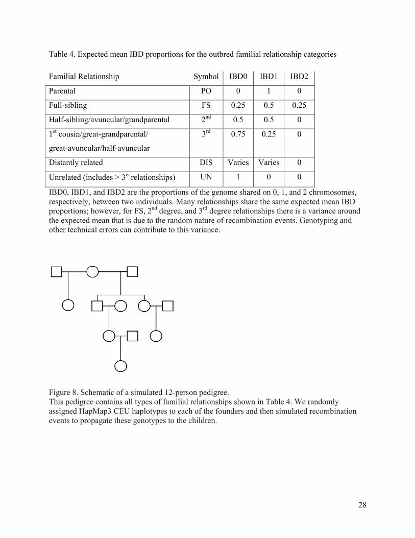
1. Size12 pedigree: a 12-person pedigree containing all relationships from Table 4 (Figure 8).
2. Uniform pedigree: a variable-sized pedigree with no half-sibling relationships in which each pair of parents is expected to have three children. However, to obtain the desired pedigree sizes, there may be a single pair of parents with as few as one child or as many as four children (Figure 9).
3. Half-sibling pedigree: identical to Uniform except there is a 30% chance that one person from each pair of parents has two children with another individual (Figure 9).
For both the Uniform and Halfsib pedigrees, we simulated complete pedigrees of sizes ranging
from five to 400 individuals. For each pedigree we created different genotypes for 100 versions
of the pedigree structures using the method applied by Morrison61 (see Web Resources): we
randomly selected founder haplotypes with ~1M SNPs from among the unrelated HapMap3
CEU samples, and we simulated recombination as a homogeneous Poisson process disregarding
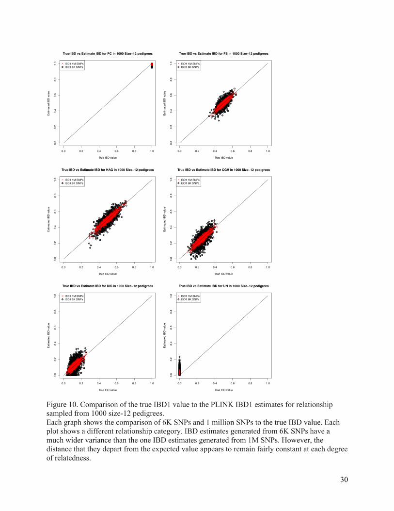
the centromere and using the approximation 1 Mb = 1 cM. We compared the true IBD
proportions to those calculated by PLINK for IBD estimates generated from 6K and 1M SNPs
(Figure 10). The correlation between the estimates and the true values were r2 = 0.999 with
pedigrees of size ten and r2 = 0.974 with pedigrees of size 400. IBD estimates generated from as
few as 6K SNPs are still remarkably accurate (Supplementary Table 1), and they improve as the
number of SNPs increases. We also tested the accuracy of IBD estimates calculated using the
overlap of the approximately one million HapMap3 SNP set and commonly used SNP panels and

27
found high accuracy levels (Supplementary Table 1). Unless otherwise stated, the complete ~1M
SNP sets were used for the simulations.
We also simulated data missingness in each of the Uniform and Halfsib pedigrees. To
accomplish this, we created ten additional versions of each pedigree by iteratively removing
genetic data for a single sample until we had removed up to ten missing individuals. Data were
eligible for removal if the individual had children and if his or her removal did not create a gap
in the pedigree larger than a 3rd degree relationship. Eligible samples were removed uniformly at
random, creating unique combinations of missing sample data for each pedigree.
28
Table 4. Expected mean IBD proportions for the outbred familial relationship categories
Familial Relationship Symbol IBD0 IBD1 IBD2
Parental PO 0 1 0
Full-sibling FS 0.25 0.5 0.25
Half-sibling/avuncular/grandparental 2nd 0.5 0.5 0
1st cousin/great-grandparental/
great-avuncular/half-avuncular
3rd 0.75 0.25 0
Distantly related DIS Varies Varies 0
Unrelated (includes > 3° relationships) UN 1 0 0
IBD0, IBD1, and IBD2 are the proportions of the genome shared on 0, 1, and 2 chromosomes, respectively, between two individuals. Many relationships share the same expected mean IBD proportions; however, for FS, 2nd degree, and 3rd degree relationships there is a variance around the expected mean that is due to the random nature of recombination events. Genotyping and other technical errors can contribute to this variance.
Figure 8. Schematic of a simulated 12-person pedigree. This pedigree contains all types of familial relationships shown in Table 4. We randomly assigned HapMap3 CEU haplotypes to each of the founders and then simulated recombination events to propagate these genotypes to the children.

29
Figure 9. Examples of simulated pedigrees of size 20. A) Uniform size-20 pedigree with five samples for whom the genetic data was removed. The missing individuals simulated the real world case where you cannot get good genotypes from an individual either due to lack of consent, poor DNA quality, contamination, or absence of the individual. All of the remaining individuals are genotyped and are included in the pedigree and the reconstruction. B) Halfsib size-20 pedigree without any missing individuals.
30
Figure 10. Comparison of the true IBD1 value to the PLINK IBD1 estimates for relationship sampled from 1000 size-12 pedigrees. Each graph shows the comparison of 6K SNPs and 1 million SNPs to the true IBD value. Each plot shows a different relationship category. IBD estimates generated from 6K SNPs have a much wider variance than the one IBD estimates generated from 1M SNPs. However, the distance that they depart from the expected value appears to remain fairly constant at each degree of relatedness.
●●●●●
●●●●●●●●●●●●●●●●●●●●●●●
●
●●●●
●
●
●
●●●●
●
●●●●●●●●●●●●●●●●●●●●●●●●●●●●●
●●●●●●●●●●●●●●●●●
●●●●●●●●●●●●●●●●●●●●●●●
●
●●●
●
●●●●●●●●●●●●●●●●●●
●
●
●●●●●
●●●●●●●●
●●●●●●●●●●●●●●●●●●●●●●●●●●●●●●●●
●●●●●●●●●●●●●●●●●●●●●●●
●
●●●
●
●●●●●●●●●●●●●●●●●●●●●●●●●●●●●
●●●●●●●
●
●●●●●●●●●●●●●●●●●●●●●●●
●●
●
●●●●●●●●●●●●●●●●●●●●●●●●●●●●●●●●●●●●●●●●●●●●●●●●●●●
●
●●●●
●●●●●●●●●●●●●●●●●●●●●●●●●●●●
●●●
●●●
●●●●
●
●●●●●●●●●●●●●●●●●●●●●●●●●●●●●●●●●●●●●●●●●●●●●●●●●●●●●●●●●●●
●
●●●●●●●●●●●●●●●●●●●●●●●●●●●●●
●●●●●●●●●●
●
●●●●●●●●●
●
●●●●●●●
●
●●●●●●●
●
●●●●●●●●●●
●
●●●●●●●●●●●●●●●●●●●●●●●●●●●
●
●●●●●●●●●●●●●●●●●●●●●●●●
●●●●
●●●
●
●●●●●●●●●●●●●●●●●●●●●●●●●●●
●
●●●●●●●●●●●●●●●●●●●●●●●●
●
●●●●●●●●●●●●●
●●
●
●
●●●●●●●●●●●●●●●●●●●●●●●●●●●●●●●●●●●●●●
●
●●●●●●●●●●●●●●●●●●●●●●●●●●●●●●●●●●●●●●●●●●●
●
●●
●
●●●●●●●●●●●●
●
●●●●●●●●●●
●●●●●●●●●●●●●●●●●●●●●●●●●●●●
●
●●●●●●●●●●●●●●●●●●
●
●
●●●●●●●
●●●●●●●●●●●●●●●●●
●
●●●●●●●●●●●●●●●●●●●●●●●●●●●●●●●●●●●●●
●
●
●●●●●●●●●●●
●
●●●●●●●●●●●●●●●●●●●●●●●●
●●●●●●●●●
●●●●●●●●●●●●●●●●●●●●●●●●●●●●●●●●●●●●●●●●●●●
●
●●●●●●●●●●●●●●●●●●●●●
●
●●●●●●●●●●●●●●●●●●●●●●●●●●●●●●●●●●
0.0 0.2 0.4 0.6 0.8 1.0
0.0
0.2
0.4
0.6
0.8
1.0
True IBD vs Estimate IBD for PC in 1000 Size−12 pedigrees
True IBD value
Estim
ated
IBD
val
ue
●
IBD1 1M SNPsIBD1 6K SNPs
●
●●
●
●
●
●
●●
●
●
●
●●
●●
●
●
●
●●
●
●●
● ●
●
●●●●
●
●
●
●
●●
●●
●
●
●●
●
●
●
●
●
●●
●
●
●
●
●
●
●
●●
●
●
●
●
●
●
●
●
●
●●
●●
●
●
●●●
●
●
●
●
●●
●
●●
●
●
●●
●
●
●
●
●●
●
●
● ●
●
●
●
●
●
●
●●
●
●
●●
●
●
●
●
●
●●
●
●●●●●
●
●
●
●
●
●
●
●
●
●
●
●
●
●
●●●
●
●
●
●
●
●
●
●
●
●
●
●
●●
●
●
●●
●
●
●● ●
●
● ●
●
●
●
●●●
●
●●
●
●
●
●
●●
●
●
●
●
●
●●
●●
●
●●
●
●●
●
●
●
●●
●
●
●
●●
●
●
●●
●
●
●●
●
●
●
●
●
●●●
●
●
●
●
●
●
●
●
●
●
●●
●
●
●
●
●
●
● ●
●●
●
●
●●
●
●
●●
●
●
●●
● ●●●
●
●
●
●●
●
●
●
●
●
●
●
●
●●
●
●●
●●
●
●
●
●
●
●●
●
● ●
●●
●
●
●
● ●
●
●
●●
●●
●
●
●
●●
●
●●
●
●
●
●
●
●
●● ●
●
● ●●
●
●
●
●
●
●●
●
●
●
●
●
●●
●
●
● ●●
●
●
●
●
●
●
●
●
●
●
●
●●
●
●
●
●
●
●
●
●
●
●
●●
●
●
●
●
●●
● ●
●
●
●
●
●
●
●
●
●
●
●
●
●
●
●●
●
● ●
●● ●
●
●
●
●
● ●●
●
●
●
●
●●●
●
●
●
●
●
●
●●
●
●●
●●
●
●●
●
●
●
● ●
● ●
●●
●●●
●
●
●
●●
●●
●
●
●
●
●
●●
●
●
●
●
●
●●
●●
●
●●
●
●
●
●●
●
●
●
●●●
●
●●
●
●
●
●
●●
●
●
●
●
●
●
●
●●
●
●
●
●●
●
●
●
●
●
●
●
●
●
●●
●
●
●
●
●
●
●●
●●
●
●●●
●
●
●
●
●
●
●●
●
●
●
●●
●●
●
●●
●●
●
●●●
●
● ●
●
●●●●●
●●
●
●
●
●●
●
●●
●
●
●
●
●
●●●
●
●
●
●
●●●
●
●●●
●
●
●
●
●
●●
●
●
●
●
●●
●●
●
●
●
●
●●
●
●●
●
●●
●
●
● ●●
●●
●
●●●
●
●●
●
●
●●
●
●
●
●
●
●
●
●
●
●
●
●
●
●
●
●●
● ●
●
●
●
●
●
●●●
●
●
● ●
●
●
●
●● ●
●
●●
●
●
●●
●
●
●
●●
●
●●
●
●
●
●
●
●
●
●●
●
●
●
●
●
●
●
●
●
●●
●
●
●
●●
●●
●
●
●
●
●●
●
●
●
●
●
●
●●
●
●●●
●
●
●
●
●
●
●
●●
●
●
●
●
●
●
●●
●
●
●
●
●
●
● ●
●
● ●
●●
●
●
●
●
●
●●●
●
●●
●●●
●
●
●●
●
●●
●
●●
●
●
●
●
●
●
●●● ●
●
●
●
●
●
●● ●
●
●
●
●
●●
●
●
●
●
●
●
●
●
●
●
●
●
●
●
●
●
●
●●
●
●
●
●
●
●
●
●
●
●●
●
●
● ●
●
●
●●
●
●
●
●
●●
●
●
●●
●
●
●●
●
●
●●
●
●
●●
●
● ●●
●
●
●
●
●
●
●
●
●●
●
●●
●●
●
●
●●● ●
●
●●
●● ●
●
●
●
●
●
●
●
●
●
●
●
●
●
●
●
●
●
●●●●
●
●● ●
●
●
●
●
●
●
●●
●
●
●
●
●●
●
●
●
●
●
●
●
●
●
●
●
●
●
●●
●
● ●
●●
●
● ●
●
●● ●
●
●
●
●●
●●
● ●
●
●
●
●
●
●
●
●
●●
●
●●
●
●
●
●●
● ●
●●
●
●●
0.0 0.2 0.4 0.6 0.8 1.0
0.0
0.2
0.4
0.6
0.8
1.0
True IBD vs Estimate IBD for FS in 1000 Size−12 pedigrees
True IBD value
Estim
ated
IBD
val
ue
●
IBD1 1M SNPsIBD1 6K SNPs
●
●
●
●
●
●
●
●
●
●●●
●
●
●
● ●●
●●
●
●
●
●
●
●
●
●
●
●
●
●
●
●
●
●
●
●
●
●●
●
●●
●
●
●
●
●
●
●
●
●
●
●
●
●
●
●
●
●
●
●
●
●
●●
●
●
●
●
●
●
●
●
●●
●
●
●
●
●
●●
●
●
●
●
●
●
●
●
●
●
●
●
●
●
● ●
●●
●
●
● ●●
●
●
●●
●
●
●●
●●
●
●
●
●●
●
●
●
●
●
●
●
●
●
●
●
●
●
●●
●
●
●
●
● ●●
●
●
●
●
●●
●
●
●
●
●
●
●
●
●
●
●●
●
●
●●
●
●
●
●●
●●● ●
●●
●
●
●
●
●●
●
●
●
●
●
●
●
●●
●
●
●
●
●
●
●
●
●●
● ●
●
●
●
●
●
●
●
●
● ●
●●
●
●
●
● ●●●
●●●
●
●●
●
●
●
●●
●●
●
●
●
●
●
●
●
●●●
●
●
●
●
●
●
●●
●
●
●
●
●
●
● ●●
●
●
●●
●
●
●●
●
●●
●
●
●
●●
●
●
●
●
●
●
●
●
●
●
●
●
●●●
●
●
●
●
●
●
●
●
●
●●
●
●●
●
●
●●
●
●
●
●●
●●
●
●
●
●
●
●
●
●●
●
●
●●
●
●
●
●●
●
●●●
●
●
●
●
●
●
●
●●
●●
●
●
●
●
●
●
●
●
●
● ●
●
●
●
●
●
●
●
●
●
●
●
●
●
●
●
●●
●
●
●
●
●
●
●
●
●
●
●
●
●
●
●
●
●
●
●
●
●
●
●
●
●
●
●
●
●
●
●
●
●
●
●
●
●
●
●
●●
●
●
●
●
●
●
●
●
●
●
●
● ●
●
●
●
●
●
●
●
●
●
●
●
●
●
●
●
● ●
●
●
●
● ●
●
●
●
●
●●
●
●
●
●
●●
●●
●
●
●●
●●
●
●
●
●
●
●
●
●
●●
●
●
●
●
●
●●
●
●
●
●●
●
● ●
●
●
●
●
●
●
●
●
●
●
●●
●
●
●
●●
●
●
●
●
●●●●
●
●
●
●
●
●
●
●
●●
●
●
●
●
●
●
●
●●
●
●
●●
●
●
●
●
●
●
● ●
●
● ●
●●
●
●
●
●
●
●
●
● ●●
●●
●
●●
●
●
●
●
●
●
●●
●●
●
●
●
●
●
●
●
●
●
●
●
●
●
●
●
●
●
●
●●
●
●●
●
●
●
●
●
●
●
●●●
●
●
●
●
●
●
● ●
●
●
●●●●
●
●
●
●
●
●
●
●
●
●
●
●
●
●
●
●
●
●
●
●
●
●●
●
●
●
●
●●
●● ●
●
●
●
●
●
●
● ●●
●
●
●●
●●
●
●
●
●
●
●
●
●● ●
●
●
●
●
●
●
●
●
●
●●
●
●
●
●
●●
●
●
●
●
●●
●
●
●
●
●
●
●
●
●
●
●
●
●
●
●
●●
●
●
●
●
●
●●
●
●
●
●
●
●
●
●
●
●
●
●
●
●
●●
●
●
●
●
●
●
●
●
●
●
●
●
●
●
●
●●
●
●
●●
●
●
●
●
●
●
●
●●
●
●
●
●
●
●
●
●
●
●
●
●
●
●
●●
●
●
●
●
●
●
●●
● ●
●
●
●
●
●
●
●
●
●●
●●
●
●
●●
●●●
●
●
●
●
●
●
●
●
●
●
●
●
●●
●
●
●
●
●
●
●
●
●
●
●
●
●
●
●
●●
●
●
●
●
●
●
●
●
●
●
●
●
●●
● ●
●
●
●
●
●
●
●
●
●
●●
●
●
●
●
●
●
●●
●
●
●
●
●
●
●
●
●
●
●
●
●
●
●
●
●
●
●
●
●
●●
●
●
●
●
●
●
● ●
●
●
●
●
●
●
●●
●
●
●
●●
●
●
●●
●●
●
●
●
●
●
●
●
●●
●●
●
●●
●
●
●
●
●
●●
●
●
●●
●
●
●●
●
●
●
●
●
●
●
●
●
●
●
●
●
● ●
●
●
●
●
●
●●
●
●
●
●
0.0 0.2 0.4 0.6 0.8 1.0
0.0
0.2
0.4
0.6
0.8
1.0
True IBD vs Estimate IBD for HAG in 1000 Size−12 pedigrees
True IBD value
Estim
ated
IBD
val
ue
●
IBD1 1M SNPsIBD1 6K SNPs
●
●
●●
●●
●●
●●
●
●
●●
●
●
●
●
●
●
●●
●●
●
●
●
●
●
●●
●
●
●
●
●
●
●
●
●●
●
●●
●●
●
●●
●●●
●
●●
●●
●
●
●
●
●●
●● ●
●
●
●●
●
●
●
●
●
●
●
●
●
●
●
●
●
●
●
●
●
●
●
●
●
●
●
●
●
●
●●
●
●
●
●
●
●●
●
●
●
●
●
●
●
●
●
●
●●
●●
●
●
● ●●●
●
●
●
●
●
●
●
●
●
●
●
●
●●
●
●
●
●
●
●
●
●
●
●
●
● ●
●
●
●
●
●
●
●
●
●
●
●
●●●
●
●●
●
●
●
●
●
●
●
●
●
● ●
●
●
●●
●
●
●
●
●●
●
●
●
●
●
●
●
●
●
●
●
●
●
●
●
●
●
●●
●
●
●
● ●
●
●
●
●
●●
●●
●
●
●●
●●●
●
●
●
●●
● ●
●
●
●
●
●
●
●●
●
●
●
●●●
●●
● ●
●
●
●
●
●
●
●
●
●
●
●
●
●
●
●●
●
●
●
●●
●
●
●
●
●
●
●
● ●
●
●
●
●
●
●
●●
●
●
●
●
●
●
●
●
●
●
●
●
●
●
●
●
●
●
●
●
●
●
●●
●●
●
●
●
●
●●
●
●
●
● ●
●
●
●
●
●
●
●
●
●
●
●
●
●●●
●
●
●●●
●
●
●
●
●
●
●
●
●
●
●
●
●
●
●
●
●●
●
●●
●
●
●●
●
●
●
●
●
●
●
●
●
●
●
●
●
●
●
●
●
●
● ●
●
●
●●●
● ●
●●
●
●
●
●
●
●
●
●
●●
● ●
●
●
●
●
●●
●
●
●
●
●
●
●
●
●
●●
●
●
●
●
●
●
●
●
●
●
●
●
●
●
●
●
●
●
●
● ● ●●
●
●
●
●
●
●
●●
●
●●
●
●
●
●●
●
●
●
●
●●
●
●
●
●
●
●
●
●
●
●
●
●
●●
●
●
●
●●●●
●
●
●
●
●
●
●
●
●
●
●●
●
●
●
● ●
●
●
●●
●
●●
●
●
●
●
●
●
●
●
●
●
●
●
●
●
●●
●
●
●
●
●
●
●
●
●●
●
●●
●
●
●
●●
●
●
●●
●
●
● ●●●
●
●
●●●
●●
●●
●
●
●
●
●
●
●
●
●
●
●
●
●●●●
●
●
●
●
●●
●
●
●
●
●
●
●
●
●
●
●
●●
●●
●●
●
●
●●
●
●
●
●
●
●
●
●
●
●
●
●
●
●●
●
●●
●
●● ●
●
●
●
●
●
●
●
●
●
●
●
●●
●
●
●
●
●
●●
●
●
●
●●
●●●
●
●
●●
●
●
●●
●●
●
●
●
●
●
●
●
●
●
●
●●
●
●
● ●
●
●
●
●
●
●
●
●
●
●●
●●
●
●
●
●●
●
●
●
●●
●
●●
●
●
●
●●
●●
●●
●
●
●
●
●
●
●
●
●
●
●
●
●
●●
●
●
●
●
●
●
●
●
●
●
●
●
●
●
●
●●
●
●
●
●
●
●
●●
●
●●●
●
●●●
●
●
●
●
● ●
●
●
●
●
●
●
● ●
●
●
●●
●
●
●
●
●
●
●
●
●
● ●●
●
●
●
●
●●●
●
●
●
● ●
● ●●
●
●
●
●●
●
●
●
●
●●
●
●
●
●
●
●
●
●
●
●
●
●●
●
●●
● ●
●
●●
●●
●
●
●
● ●
●
●●
●
●
●
●
●
●
●●
●
●
●
●
●
●●
●●
●
●
●
●
●
●
●
●●
●
●
●●
●
●●
●
●
●●
●●●
●● ●
●
●●
●
●
●
●
●
●
●
●●
●●
●
●
●
●
●●
●
●
●●
●
●
●
●
● ●
●
●
●
●
●
● ●●
● ●
●
●
●
●
●
●
●●
●●
●
●●
●
●
●
●
●
●
●
●
●
●
●●
●
●
●
●
● ●
●
●
●
●
●●
●
●
●
●
●
●
●
● ●
●●
●
●
●
●
●
0.0 0.2 0.4 0.6 0.8 1.0
0.0
0.2
0.4
0.6
0.8
1.0
True IBD vs Estimate IBD for CGH in 1000 Size−12 pedigrees
True IBD value
Estim
ated
IBD
val
ue
●
IBD1 1M SNPsIBD1 6K SNPs
● ●
●
●
●
●●
●
●
●●
●
●
●
●
●●
●
●
●
●
●
●
●
●
●
●
●
●
●●
●
●
●
●
●
●
●
●
●
●●
●
●
●
●●
●
●●
●
●
●
●
●
●
●
●
●
●
●
●
●
●
●
●
●
●
●
●●
●
●
●
●●
●
●●
●
●
●
●●
●
●
●●
●●
●
●●
●●
●
●●
●
●
●
●
●
●
●
●
●
●
●
●
●
●
●●
●
●
●
●
●
●●
●
●●
●
●
●
●●
●
●●
●●
●
●
●
●
● ●
●
●
●
●
●
●
●
●●
●
●
●●
●
●
●
●●
●●
●
●
●
●●
●
●
●
●
●●
●
●
●
●●●
●
●
●
●
●
●
● ●
●
●
●
●
●●
●
●
●
●● ●
●● ●
●
●
●
●
●
●
●●
●
●
●
●
●
●
●●
●
●
●
●
●
●
●●●
●
●
●
● ●●
●
●
●●●
●
●●
●
●
●●
●
●
●
●
●
●
●
●●
●
●
●
●●
●
●●
●
●
●
●
●
● ●
●
●
●
●●
●
●
●
●●
●
● ●
●
●●
●
●
●
●
●●
●
●
●●
●
●
●
●
●
●
●
●
●
●●
●
●●
●
●
●
●
●
●
●
●
●
●●
●
●
●
●
●
●
●
●
●●
●
●
●
●
●
●
●
●
●
●
●
●
●
●● ●●
●●●
● ●
●
●
●
●
●
●
● ●●
●
●
●
●
●
●
●
●
●
●
●
●
●
●
● ●
●
●
●●●
●
●
●
●●
●
●
●
●
●
●
●
●
●
●
●
●
●●
●
●
●
●●
●
●●●
●
●
● ●
●
●
●●
●
●
●
●
●
●
●
●
●
●●
●●
●● ●
●
●
●
●
●
●●
●
●
●●
●
●
●
●
●
●
●
●
●
●
●
●
●
●
●
●
●
●
●
●●
●
●●
●
●
●
●
● ●●●
●
● ●
●
●
●
●
●
●
●
●
●
●
●
●
●
●
●●
●
●
●●●
●
●
●
●
●
●
●●
●
●
●
●
●
●
●
●
●●
●●
●●
●
●
●●●
●●
●
● ●
●
●●
●
●
●
●
●
●
●
●
●
●
●●
●
●
●
●
●
●
●
●
●
●●
●
●
●
●
●
●
●
●
●
● ●●
●
●
●
●●
●
●
●
●
●
●
●
●
●
●
●
● ●●●
●
●
●●
●
●
●
●
●●
●
●
●
●●
●
●
●●
●
●
●
●●●
●
●
● ●●
●
●●
●
●
●
●●
●
●
●
●
●
●
●
●
●
●
●●
●
●
●
●
●
●●
●
●
●
●
●
●
●●●
●
●
●
●
●
●●●
●●
●
●
●
●
●
●
●
●
●
●
●
●
●
●●
●
●●
●
●
●
●
●
●
●
●
●
●
●●
●
●
●
●
●
●
●
●●
● ●
●
●
●
●
●
●
●
●
●
●
●●
●
●
●
●●
●
●
●
●
●●
●
●
●
●
●●●
●●
●
●
● ●
●
●
●
●
●●
●
●
●
●● ●
●
●●
●
●
●
●
●●
●●
●
●
●●
●
●
●
●
● ●●
●●●
●
●
●
●
●
●
●
●
●
●
●
●●
●
●● ●
●
●
●
●
●
●
●
●●
●●
●
●
●
●●
●
●
●
●
●
●
●
●
●
●
●
●
●
●●
●●
● ●
●
●
●
●
●
●
●
●
●
●●
●
●
●
●
●●
●
●●●
●
●
●
●
●
●
●
●
●
●
●●
●
●
●
●
●
●
●●
●
●
●
●
●
●
●
●
●
●
●
●
●
●
●
●●
●
●
●●
●
●
●
●
●
●
●
●●
●
●
●●
●
●
●
●●
●
●●
●
●
●
●
●
●
●
●
●
●●
●
●●
●
●
●
●
●
●
●
●●
●
●
●
●
●
●
●
●
●●
●
●●
●
●
●
●
●
●●
●●
●
●
●
●
●
●
●
●
●●
●
●
●
●
●
●
●
●
●
●
●
●●
●●
●
●
●●
●
●
●
●
●
●
●
●
● ●●
●
0.0 0.2 0.4 0.6 0.8 1.0
0.0
0.2
0.4
0.6
0.8
1.0
True IBD vs Estimate IBD for DIS in 1000 Size−12 pedigrees
True IBD value
Estim
ated
IBD
val
ue
●
IBD1 1M SNPsIBD1 6K SNPs
●
●
●●●
●
●
●●
●●●●●
●●
●
●
●●●
●
●
●
●●●●●●
●●
●●
●
●
●●
●●●●
●●
●
●●●●●●●●
●●●
●
●
●
●●
●●●
●
●●
●
●●●
●●
●
●
●
●
●●●●●●●●●●●●●
●
●●●●●●
●
●●●●
●
●●●●
●
●●●
●●●●
●
●
●●
●●
●●
●●●
●
●
●
●●
●
●●
●
●●
●
●
●
●●
●
●●●
●
●
●
●
●
●
●●●●
●
●
●
●
●
●●
●
●●
●●●
●
●●●
●●
●
●
●
●
●
●
●
●●
●
●
●●
●
●●●
●
●●
●
●●
●●
●
●
●
●
●
●
●
●
●
●●
●
●
●●●●●●
●
●●
●
●
●●
●●
●●
●
●
●
●
●●●●●●●●
●
●●●●●●●
●
●●
●
●●●●●●●●
●
●
●●●
●
●●
●●
●●
●
●
●
●
●●
●●●●●●●●
●
●●●●
●
●●
●●
●●●●●●●
●
●
●●
●
●
●
●
●
●●●●●
●
●●●●●
●
●
●
●
●
●
●●●
●
●●●
●●
●
●●
●●●●●
●●●
●
●
●
●
●
●
●
●●●●●●
●
●
●
●
●
●●
●
●●●
●
●●
●●●
●●
●
●
●
●●
●●
●●●●●●●●
●
●
●
●●●●●●●
●
●●
●●
●
●●●●
●
●
●
●
●
●
●
●
●●●●●●●●●
●
●●●
●●●●
●
●●●●●●●●●
●
●●
●●
●
●
●●
●●
●
●●
●●●
●
●
●
●●
●
●●●
●
●●
●
●
●
●
●
●●●●●●●●●●●●●●●●●●
●
●●
●
●●●●
●●●●●●
●
●●
●
●●●
●
●●●●●●●●
●
●●●
●
●
●
●●
●
●●●●
●
●●
●●
●
●
●
●●●●●
●
●
●
●●
●
●
●
●●
●●●
●
●
●
●
●
●●●●
●
●
●
●●●●
●●
●
●
●●●
●
●
●
●●
●
●
●
●●●●●●
●
●
●●
●
●
●
●
●
●●●
●
●●
●
●
●
●●●
●
●●●
●
●
●●●●●●●●●●
●
●
●
●●
●
●
●
●●
●●
●●●●●●●●
●
●●●●
●
●●
●
●
●●
●
●●●●
●
●●●
●●●
●
●
●
●
●●
●●●●
●
●
●
●
●
●
●
●
●
●●●
●
●
●
●
●
●●●●
●
●
●
●
●
●
●●
●
●
●
●
●●
●●●●●●●●●●●●●●●●●
●
●
●●●●●●●●
●
●●●●
●
●
●●●
●
●●●●
●
●
●
●●●●●●●●●●●
●
●●●●●●●●●●●●
●
●
●●
●●●●●●
●
●●●
●
●●
●
●●●
●
●●●●●●●●●●
●
●
●
●
●●●●
●
●●
●
●●
●
●●●●●
●
●
●
●●
●
●
●
●
●●●●
●
●●●●
●
●●●●●●●●●●●●●●●●●
●
●●●●●
●
●●●●●●●●●●●●●
●
●
●
●●●
●
●
●
●●
●
●●
●
●
●
●●
●
●
●
●
●●
●●
●
●
●
●
●●●●●●
●
●
●●
●●
●●●
●
●●●
●
●
●
●
●●●
●
●
●
●
●
●●●●●
●●
●●●●●●●●●●●●●●●●
0.0 0.2 0.4 0.6 0.8 1.0
0.0
0.2
0.4
0.6
0.8
1.0
True IBD vs Estimate IBD for UN in 1000 Size−12 pedigrees
True IBD value
Estim
ated
IBD
val
ue
●
IBD1 1M SNPsIBD1 6K SNPs

31
IBD estimates
PRIMUS takes input from any program that provides estimates of the proportions of the genome
shared IBD on 0, 1, and 2 chromosomes (IBD0/1/2). We note that calculating accurate
relationships and estimating pairwise IBD is a non-trivial problem, and one that has been tackled
by a number of methodologies23; 25; 42; 62; 63. IBD proportions presented here were calculated
using the method of moments estimation implemented in PLINK23. Although not required for the
simulated pedigrees, some pedigrees may require careful analysis of admixture in the samples. In
these cases, we applied the approaches recommended by Morrison61 to remove ancestry
informative SNPs that could otherwise bias IBD estimates. The code used to calculate IBD
estimates is available for download with the PRIMUS package (Web Resources).
Family network identification
PRIMUS first groups the samples into family networks (or groups) based on the estimated
pairwise coefficient of relatedness (two times the kinship coefficient)18. An individual is only
added to a family network if the sample is related to at least one other person in the network
given a user-defined minimum coefficient of relatedness. For example, 0.1875, the midpoint
between the mean expected IBD proportion for 2nd and 3rd degree relatives, is a threshold that
will capture connections between most 2nd degree relatives or closer. The pedigree reconstruction
is then performed independently on each family network within the dataset.
Familial relationship prediction using a kernel density estimation (KDE) function
PRIMUS uses six relationship categories to reconstruct pedigrees based on the expected mean
IBD0/1/2 shown in Table 4; however, distantly related and unrelated samples are handled as the
same class during reconstruction. Both biological (i.e., recombination events, population
substructure, historic inbreeding) and technical (i.e., density and distribution of the genotyped
markers) factors contribute to variation around these means.
Given the IBD0, IBD1, and IBD2 estimates for a pair of individuals, PRIMUS predicts the
corresponding relationship category using a trained kernel density estimate (KDE; see Web
Resources) for each of six familial relationship categories. We chose to use the KDEs to account
for the overlapping IBD distributions and the variability of the IBD estimates. We used the

32
scipy.stats.gaussian_kde function (Web Resources) with two training features: genome-wide
estimates of IBD0 and IBD1. The training IBD0 and IBD1 estimates were selected from the IBD
estimates generated with 6K SNPs for the 1,000 Size12 simulated pedigrees. We chose to use the
lower number of SNPs so that the KDE could better handle the technical noise that comes with
estimating IBD. A parent/child, full-sibling, 2nd degree, 3rd degree, distantly related, and
unrelated relationship were selected from each of the 1,000 simulated pedigrees and were used to
train the respective KDEs. We used these simulated IBD proportions to train a KDE function for
each of the six familial relationship categories.
Since the coefficient factor influences the trained KDE, we tested each KDE with different
values for the coefficient factor used in calculating the kernel covariance matrices and the results
are in Figure 11. Evaluated the performance of each KDE by calculating the false positive (FP)
and false negative (FN) relationship predictions when trained with different coefficient factors.
We used these predictions to optimize the ability of PRIMUS to accurately identify the
relationship between two individuals (true positive = 1 - FN) while minimizing the number of
incorrect relationships that it predicts (FP). Since the optimal bandwidth would need to perform
well across different likelihood cutoffs, we tested the performance of PRIMUS with likelihood
cutoffs ranging from 0.01 to 0.5. We used the scipy.stats.gaussian_kde function (Web
Resources) with two training features: genome-wide estimates of IBD0 and IBD1. We tested a
range of bandwidths by specifying scalar values 1 through 17 as the “bw_method” option and
these values are used as the coefficient that multiplies the data covariance matrix to obtain the
kernel covariance matrix. With KDEs trained at each bandwidth coefficient value from 1 to 17,
we predicted the relationship category of each relationship in the 100 Uniform size-400
pedigrees at likelihood cutoffs varying from 0.01 to 0.5. We evaluated the relationship prediction
of the KDEs trained with different bandwidths by testing their FN (results A-E) and FP (results
F-J) rates.
The results can bee seen in Figure 11. The color in each cell indicates the number of
relationships from the 100 size-400 Uniform pedigrees that were either FN or FP. The color scale
is log10. An FN occurs if the true relationship did not have a likelihood higher than the cutoff. An
FP occurs if a relationship other than the true relationship has a likelihood higher than the
likelihood cutoff. Parent-offspring relationships did not have any FP or FN predictions, so the
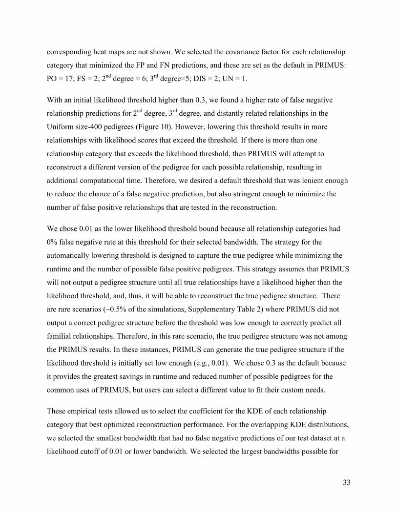
33
corresponding heat maps are not shown. We selected the covariance factor for each relationship
category that minimized the FP and FN predictions, and these are set as the default in PRIMUS:
PO = 17; FS = 2; 2nd degree = 6; 3rd degree=5; DIS = 2; UN = 1.
With an initial likelihood threshold higher than 0.3, we found a higher rate of false negative
relationship predictions for 2nd degree, 3rd degree, and distantly related relationships in the
Uniform size-400 pedigrees (Figure 10). However, lowering this threshold results in more
relationships with likelihood scores that exceed the threshold. If there is more than one
relationship category that exceeds the likelihood threshold, then PRIMUS will attempt to
reconstruct a different version of the pedigree for each possible relationship, resulting in
additional computational time. Therefore, we desired a default threshold that was lenient enough
to reduce the chance of a false negative prediction, but also stringent enough to minimize the
number of false positive relationships that are tested in the reconstruction.
We chose 0.01 as the lower likelihood threshold bound because all relationship categories had
0% false negative rate at this threshold for their selected bandwidth. The strategy for the
automatically lowering threshold is designed to capture the true pedigree while minimizing the
runtime and the number of possible false positive pedigrees. This strategy assumes that PRIMUS
will not output a pedigree structure until all true relationships have a likelihood higher than the
likelihood threshold, and, thus, it will be able to reconstruct the true pedigree structure. There
are rare scenarios (~0.5% of the simulations, Supplementary Table 2) where PRIMUS did not
output a correct pedigree structure before the threshold was low enough to correctly predict all
familial relationships. Therefore, in this rare scenario, the true pedigree structure was not among
the PRIMUS results. In these instances, PRIMUS can generate the true pedigree structure if the
likelihood threshold is initially set low enough (e.g., 0.01). We chose 0.3 as the default because
it provides the greatest savings in runtime and reduced number of possible pedigrees for the
common uses of PRIMUS, but users can select a different value to fit their custom needs.
These empirical tests allowed us to select the coefficient for the KDE of each relationship
category that best optimized reconstruction performance. For the overlapping KDE distributions,
we selected the smallest bandwidth that had no false negative predictions of our test dataset at a
likelihood cutoff of 0.01 or lower bandwidth. We selected the largest bandwidths possible for

34
parent/offspring and full-sibling without overlap of the density distributions with other
relationship categories. This minimizes the false positive calls for these predictions. Figure 12
shows a density plot for the KDE of each relationship category, which is consistent with previous
reports of genome-wide IBD proportions64.
PRIMUS uses the trained kernels to predict the familial relationship category for each pairwise
relationship. For a set of IBD0/1/2 proportions, PRIMUS queries each kernel for the density at
the IBD0 and IBD1 values and stores the density for each familial category in a vector. Then
PRIMUS normalizes the vector by dividing each density by the sum of all densities, producing a
vector of the likelihoods corresponding to each familial category. This relationship likelihood
vector is used during both reconstruction and ranking of possible pedigrees.
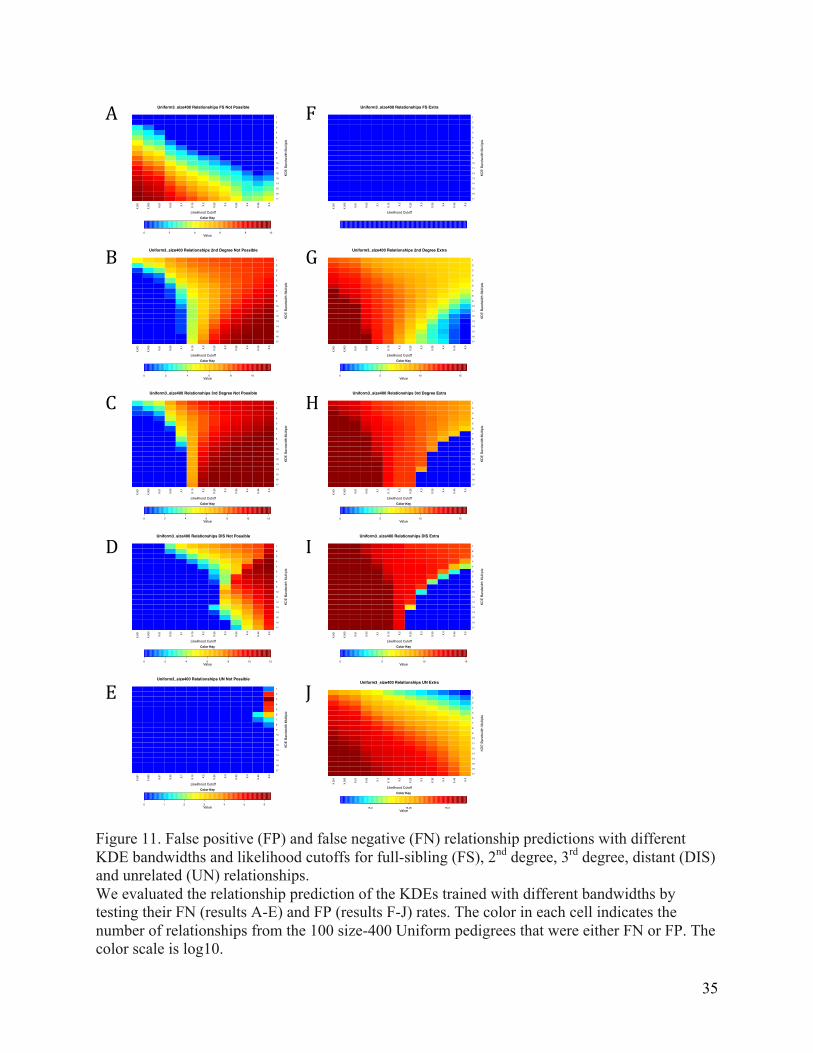
35
Figure 11. False positive (FP) and false negative (FN) relationship predictions with different KDE bandwidths and likelihood cutoffs for full-sibling (FS), 2nd degree, 3rd degree, distant (DIS) and unrelated (UN) relationships. We evaluated the relationship prediction of the KDEs trained with different bandwidths by testing their FN (results A-E) and FP (results F-J) rates. The color in each cell indicates the number of relationships from the 100 size-400 Uniform pedigrees that were either FN or FP. The color scale is log10.
X.00
1
X.00
5
X.01
X.05 X.1
X.15 X.2
X.25 X.3
X.35 X.4
X.45 X.5
Likelihood Cutoff
17
16
15
14
13
12
11
10
9
8
7
6
5
4
3
2
1
KDE
Band
wid
th M
ultip
le
Uniform3_size400 Relationships FS Not Possible
0 2 4 6 8 10Value
Color Key
X.00
1
X.00
5
X.01
X.05 X.1
X.15 X.2
X.25 X.3
X.35 X.4
X.45 X.5
Likelihood Cutoff
17
16
15
14
13
12
11
10
9
8
7
6
5
4
3
2
1
KDE
Band
wid
th M
ultip
le
Uniform3_size400 Relationships FS Extra
X.00
1
X.00
5
X.01
X.05 X.1
X.15 X.2
X.25 X.3
X.35 X.4
X.45 X.5
Likelihood Cutoff
17
16
15
14
13
12
11
10
9
8
7
6
5
4
3
2
1
KDE
Band
wid
th M
ultip
le
Uniform3_size400 Relationships 2nd Degree Not Possible
0 2 4 6 8 10Value
Color Key
X.00
1
X.00
5
X.01
X.05 X.1
X.15 X.2
X.25 X.3
X.35 X.4
X.45 X.5
Likelihood Cutoff
17
16
15
14
13
12
11
10
9
8
7
6
5
4
3
2
1
KDE
Band
wid
th M
ultip
le
Uniform3_size400 Relationships 2nd Degree Extra
0 5 10 15Value
Color Key
X.00
1
X.00
5
X.01
X.05 X.1
X.15 X.2
X.25 X.3
X.35 X.4
X.45 X.5
Likelihood Cutoff
17
16
15
14
13
12
11
10
9
8
7
6
5
4
3
2
1
KDE
Band
wid
th M
ultip
le
Uniform3_size400 Relationships DIS Not Possible
0 2 4 6 8 10 12Value
Color Key
X.00
1
X.00
5
X.01
X.05 X.1
X.15 X.2
X.25 X.3
X.35 X.4
X.45 X.5
Likelihood Cutoff
17
16
15
14
13
12
11
10
9
8
7
6
5
4
3
2
1
KDE
Band
wid
th M
ultip
le
Uniform3_size400 Relationships DIS Extra
0 5 10 15Value
Color Key
X.00
1
X.00
5
X.01
X.05 X.1
X.15 X.2
X.25 X.3
X.35 X.4
X.45 X.5
Likelihood Cutoff
17
16
15
14
13
12
11
10
9
8
7
6
5
4
3
2
1
KDE
Band
wid
th M
ultip
le
Uniform3_size400 Relationships 3rd Degree Not Possible
0 2 4 6 8 10 12Value
Color Key
X.00
1
X.00
5
X.01
X.05 X.1
X.15 X.2
X.25 X.3
X.35 X.4
X.45 X.5
Likelihood Cutoff
17
16
15
14
13
12
11
10
9
8
7
6
5
4
3
2
1
KDE
Band
wid
th M
ultip
le
Uniform3_size400 Relationships 3rd Degree Extra
0 5 10 15Value
Color Key
X.00
1
X.00
5
X.01
X.05 X.1
X.15 X.2
X.25 X.3
X.35 X.4
X.45 X.5
Likelihood Cutoff
17
16
15
14
13
12
11
10
9
8
7
6
5
4
3
2
1
KDE
Band
wid
th M
ultip
le
Uniform3_size400 Relationships UN Not Possible
0 1 2 3 4 5 6Value
Color Key
X.00
1
X.00
5
X.01
X.05 X.1
X.15 X.2
X.25 X.3
X.35 X.4
X.45 X.5
Likelihood Cutoff
17
16
15
14
13
12
11
10
9
8
7
6
5
4
3
2
1
KDE
Band
wid
th M
ultip
le
Uniform3_size400 Relationships UN Extra
15.2 15.25 15.3Value
Color Key
A F
B G
C H
D I
E J
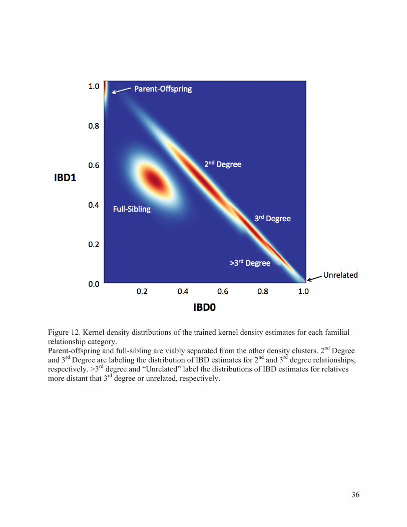
36
Figure 12. Kernel density distributions of the trained kernel density estimates for each familial relationship category. Parent-offspring and full-sibling are viably separated from the other density clusters. 2nd Degree and 3rd Degree are labeling the distribution of IBD estimates for 2nd and 3rd degree relationships, respectively. >3rd degree and “Unrelated” label the distributions of IBD estimates for relatives more distant that 3rd degree or unrelated, respectively.

37
Pedigree reconstruction algorithm
For each family network, PRIMUS uses the relationship likelihood vectors of all pairwise
relationships to reconstruct all possible pedigrees, subject to the restrictions that a) only relatives
up to 3rd degrees are considered and b) the likelihood of each relationship class considered must
exceed a minimum likelihood threshold (initial default of 0.3). We chose 0.3 as a good initial
likelihood threshold based on the relationship predictions of the Uniform size-400 pedigrees (see
Figure 11 for details).
The reconstruction is an iterative process of identifying a pairwise relationship within the family
network that has not yet been incorporated into the pedigree, fitting that relationship into the
pedigree, and testing that all of the relationships generated by adding the individual are
compatible with the relationship likelihood vectors and sex data for all of the samples. If the
addition of a relationship is incompatible with the relationship likelihood vectors or if two
individuals of the same sex have offspring, the pedigree is rejected and removed from the set of
possible pedigrees. The reconstruction continues until all pairwise relationships from the family
network are represented in each possible pedigree or until there are no possible pedigrees left to
continue reconstructing.
PRIMUS reconstructs in three phases. Phase 1 uses parent-offspring (PO) and full-sibling (FS)
relationships. These two types of relationships are the most accurately predicted because POs
have no biological variance around the expected proportion of sharing, and FS are the only non-
consanguineous relationship with IBD2 greater than 0. Phase 1 creates a backbone on which to
build the more distant relationships. A PO relationship between individuals A and B is added to
the pedigree by creating a version of the pedigree in which A is the parent of B and another
version in which B is the parent of A. Missing individuals are added as necessary so that each
individual in the family network has zero or two parents. In phase 2, PRIMUS reconstructs 2nd
degree relationships: half-sibling, avuncular, and grand-parental. The algorithm tests all possible
re-arrangements for each 2nd degree relationship within the pedigree and adds missing
individuals to connect portions of the pedigree as necessary. Phase 3 is identical to phase 2,
except that it considers 3rd degree relationships: first cousins, half-avuncular, great-avuncular,
and great-grandparental. Since PRIMUS always checks every possible way that a sample can be

38
added to the pedigree and eliminates pedigrees that do not fit, it is effectively exploring the entire
search space of possible pedigrees. At present, PRIMUS does not reconstruct complex
relationships (e.g., half-sibling plus first cousin or double 1st cousins), consanguineous
relationships, or relationships more distant than 3rd degree relatives. If one of these relationships
is present in the dataset, PRIMUS will match it to one of the relationship categories in Table 4
and fit the relationship into the pedigree accordingly.
Automatically adjusting likelihood threshold
If PRIMUS reaches the end of reconstruction and has zero possible pedigrees remaining, then it
will automatically lower the likelihood threshold from the default of 0.3 to 0.2 and will rerun,
allowing PRIMUS to consider additional possible pairwise relationships with likelihoods
between 0.2 and 0.3. PRIMUS will continue to gradually drop the likelihood threshold until it
produces a possible pedigree or it reaches a threshold below 0.01. If no possible pedigrees result
from reconstruction after lowering the threshold below 0.01, then PRIMUS stops reconstruction.
For further details, see Figure 11.
Pedigree scoring
For many families, there is only one possible pedigree that fits the data and the true pedigree.
However, due to the unknown directionality of some relationships and missing data for
individuals, PRIMUS can reconstruct more than one possible pedigree that fits the genetic data
with the true pedigree among them. We attempt to increase the chances that the true pedigree is
near the top of the list by ranking the possible pedigrees using the relationship likelihood vectors
to obtain a pedigree score.
PRIMUS will rank the pedigrees according to a pedigree score calculated by summing the log of
the likelihood value of each relationship in the pedigree. This score is used to provide a ranking
of the pedigrees. For example, if a pedigree has only two individuals, and they have a 0.6
likelihood of being 2nd degree relatives and a 0.4 likelihood of being 3rd degree relatives, then all
pedigrees where they are 2nd degree relatives will be ranked higher than pedigrees in which they
are 3rd degree relatives. Additionally, if the ages of individuals are provided, then PRIMUS will
flag and rank all pedigrees where the ages are inconsistent (e.g., a child is older than the parent).
39
PRIMUS results and output
PRIMUS uses Cranefoot65 (Web Resources) to provide an image of each pedigree and provides
the corresponding PLINK-formatted FAM file. Summary results are provided for each family
network and the entire dataset, as well as a list of the possible relationships for each pair of
related individuals similar to Supplementary Table 3. See the PRIMUS documentation for a
complete list and description of output files and formats (Web Resources).
Pedigree checking program
PRIMUS also has the ability to check that a reported pedigree is among the produced
reconstructed pedigrees. The user provides the reported pedigree in the form of a PLINK FAM
or PED file, and PRIMUS compares it to each of the reconstructed pedigrees to see if there is a
match. In the case that the reconstruction included additional samples that were not part of the
reported pedigree, PRIMUS will find the match and report that there are additional genotyped
samples included in the pedigree.
Reconstructing authentic pedigrees
We tested the ability of PRIMUS to reconstruct several different pedigrees using real genetic
data. IBD estimates were obtained from genotypes generated with a HumanCytoSNP-12
BeadChip for all available pedigrees obtained by the University of Washington Center for
Mendelian Genomics (UW CMG) with the exception of 49 pedigrees for which only exome
sequence data were generated (see Boston EOCOPD samples). UW CMG studies were approved
by the institutional review boards of the University of Washington, and informed consent was
obtained from participants or their parents. The Boston Early-onset COPD Study participants
provided written informed consent, and the Partners HealthCare Human Research Committee
approved the study.
IBD estimates for HapMap3 were generated using pHapMap3 release 2 data (Web Resources).
We used PLINK to calculate all IBD estimates using SNPs with a minor allele frequency >1%
and a call rate >90%. We used PRIMUS to identify the maximum unrelated set for each
HapMap3 population, and the allele frequencies from the unrelated samples were used for the
IBD analysis of their own respective populations.
40
The Starr County Health Studies’ Genetics of Diabetes Study is composed of 1,890 cases and
representative control samples obtained from a systematic survey in Starr County, Texas,
conducted from 2002 to 200666. However, the types of relationships and potential families in the
study were unknown. IBD estimates for the Starr County samples were generated from
genotypes called from the Affymetrix Genome-Wide SNP Array 6.066. We used PLINK to
calculate all IBD estimates using SNPs with a minor allele frequency >1% and a call rate >90%.
We used PRIMUS18 to identify the maximum unrelated set for the Starr County data, and the
allele frequencies from the unrelated samples were used for the IBD estimations. The Starr
County Health Studies’ participants provided written informed consent, and the institutional
review boards of the University of Texas Health Science Center at Houston approved the study.
Exome sequence data and corresponding pedigrees
The Boston Early-Onset Chronic Obstructive Pulmonary Disease (EOCOPD) Study67 (see Web
Resources) is an extended pedigree study of genetic susceptibility to EOCOPD. All available
first-degree relatives (siblings, parents, and children), older second-degree relatives (half-
siblings, aunts, uncles, and grandparents), and other relatives diagnosed with EOCOPD were
invited to participate in the study. For this project, 351 subjects from 49 pedigrees were
sequenced at the UW CMG.
Exome sequencing was performed (NimbleGen v2 in-solution hybrid capture and Illumina
HiSeq 2000 sequencing)68, sequences were aligned to the human reference genome (hg19)69, and
single-nucleotide and insertion-deletion variants were called with GATK70. VCFtools71 was used
to select only PASS SNPs with a minimum and maximum depth of eight and 300, respectively,
and converted to a PLINK23 formatted .ped and .map file. IBD estimates were then calculated in
PLINK using the 56,516 SNPs with a minor allele frequency >1% and a call rate >90%. SNP
allele frequencies for the IBD analysis were calculated from 81 of the 351 exome sequenced
samples that made up the maximum unrelated set as calculated by PRIMUS18 using a coefficient
of relatedness cutoff of 0.1.
41
Results
Reconstructing simulated pedigrees
To test and evaluate the performance of PRIMUS on a broad range of known pedigrees, we
simulated two types of pedigree structures (Uniform and Halfsib) of varying sizes, different
numbers of markers, and varying combinations of missing data for individuals in the pedigrees
(see Methods for details). Figure 13 shows the simulation results for reconstruction of size-20
and size-40 Uniform pedigrees with < 20% missing samples. PRIMUS reconstructed the true
pedigree as the only pedigree or the highest scoring pedigree in 89% of the simulations. For
another 5.6% of these simulations, the true pedigree was tied as the highest scoring pedigree with
one other pedigree. Only 2.5% of these simulations failed to run to completion either due to too
many possible pedigrees (>100,000), too long of a runtime (>36 hours), or using up too much
memory (e.g., exceeding 12Gb of memory). These incomplete reconstructions were then rerun
using a relatedness cutoff of 0.375 to generate partial reconstructions for each. A partially
reconstructed pedigree typically consists of two to six pieces of the larger pedigree where the
individuals are connected by 1st degree relationships. It would require connecting these pieces
with 2nd and 3rd degree relationships to achieve a complete reconstruction of the true pedigree.
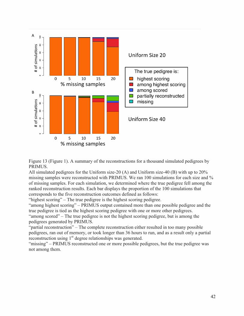
42
Figure 13 (Figure 1). A summary of the reconstructions for a thousand simulated pedigrees by PRIMUS. All simulated pedigrees for the Uniform size-20 (A) and Uniform size-40 (B) with up to 20% missing samples were reconstructed with PRIMUS. We ran 100 simulations for each size and % of missing samples. For each simulation, we determined where the true pedigree fell among the ranked reconstruction results. Each bar displays the proportion of the 100 simulations that corresponds to the five reconstruction outcomes defined as follows: “highest scoring” – The true pedigree is the highest scoring pedigree. “among highest scoring” – PRIMUS output contained more than one possible pedigree and the true pedigree is tied as the highest scoring pedigree with one or more other pedigrees. “among scored” – The true pedigree is not the highest scoring pedigree, but is among the pedigrees generated by PRIMUS. “partial reconstruction” – The complete reconstruction either resulted in too many possible pedigrees, ran out of memory, or took longer than 36 hours to run, and as a result only a partial reconstruction using 1st degree relationships was generated. “missing” – PRIMUS reconstructed one or more possible pedigrees, but the true pedigree was not among them.
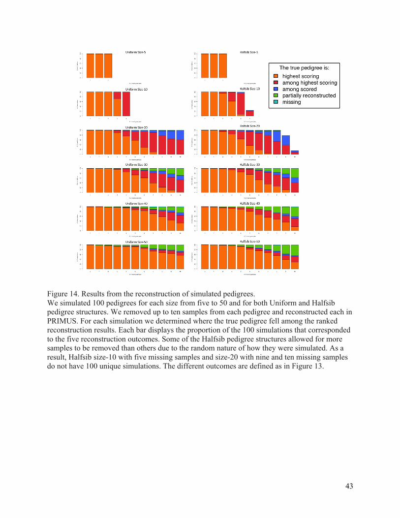
43
Figure 14. Results from the reconstruction of simulated pedigrees. We simulated 100 pedigrees for each size from five to 50 and for both Uniform and Halfsib pedigree structures. We removed up to ten samples from each pedigree and reconstructed each in PRIMUS. For each simulation we determined where the true pedigree fell among the ranked reconstruction results. Each bar displays the proportion of the 100 simulations that corresponded to the five reconstruction outcomes. Some of the Halfsib pedigree structures allowed for more samples to be removed than others due to the random nature of how they were simulated. As a result, Halfsib size-10 with five missing samples and size-20 with nine and ten missing samples do not have 100 unique simulations. The different outcomes are defined as in Figure 13.
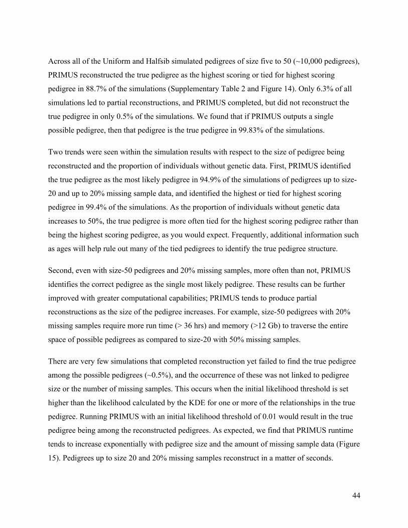
44
Across all of the Uniform and Halfsib simulated pedigrees of size five to 50 (~10,000 pedigrees),
PRIMUS reconstructed the true pedigree as the highest scoring or tied for highest scoring
pedigree in 88.7% of the simulations (Supplementary Table 2 and Figure 14). Only 6.3% of all
simulations led to partial reconstructions, and PRIMUS completed, but did not reconstruct the
true pedigree in only 0.5% of the simulations. We found that if PRIMUS outputs a single
possible pedigree, then that pedigree is the true pedigree in 99.83% of the simulations.
Two trends were seen within the simulation results with respect to the size of pedigree being
reconstructed and the proportion of individuals without genetic data. First, PRIMUS identified
the true pedigree as the most likely pedigree in 94.9% of the simulations of pedigrees up to size-
20 and up to 20% missing sample data, and identified the highest or tied for highest scoring
pedigree in 99.4% of the simulations. As the proportion of individuals without genetic data
increases to 50%, the true pedigree is more often tied for the highest scoring pedigree rather than
being the highest scoring pedigree, as you would expect. Frequently, additional information such
as ages will help rule out many of the tied pedigrees to identify the true pedigree structure.
Second, even with size-50 pedigrees and 20% missing samples, more often than not, PRIMUS
identifies the correct pedigree as the single most likely pedigree. These results can be further
improved with greater computational capabilities; PRIMUS tends to produce partial
reconstructions as the size of the pedigree increases. For example, size-50 pedigrees with 20%
missing samples require more run time (> 36 hrs) and memory (>12 Gb) to traverse the entire
space of possible pedigrees as compared to size-20 with 50% missing samples.
There are very few simulations that completed reconstruction yet failed to find the true pedigree
among the possible pedigrees (~0.5%), and the occurrence of these was not linked to pedigree
size or the number of missing samples. This occurs when the initial likelihood threshold is set
higher than the likelihood calculated by the KDE for one or more of the relationships in the true
pedigree. Running PRIMUS with an initial likelihood threshold of 0.01 would result in the true
pedigree being among the reconstructed pedigrees. As expected, we find that PRIMUS runtime
tends to increase exponentially with pedigree size and the amount of missing sample data (Figure
15). Pedigrees up to size 20 and 20% missing samples reconstruct in a matter of seconds.

45
Confirming and correcting clinically ascertained pedigrees
To demonstrate the ability of PRIMUS to verify the genetic information for clinical pedigrees,
we have reconstructed and confirmed or corrected more than a hundred pedigrees submitted to
the UW CMG. The genetic information used by PRIMUS can be derived from either chip-based
(Figure 16) or sequence-based (Figure 17 and Figure 18) technologies. Genome-wide IBD
estimates for the samples in the pedigree in Figure 16 were generated using genotypes from the
HumanCytoSNP BeadChip for each non-missing sample. PRIMUS used these IBD estimates for
all pairs of samples to reconstruct the possible pedigree. Only one pedigree fit the data, and it
matched the clinically provided pedigree, supporting our hypothesis that it is the correct
pedigree. This reconstruction took nine seconds on a 2.3 GHz Intel Core i7 processor.
Importantly, PRIMUS also introduced the five missing individuals necessary to connect the final
pedigree and correctly identified a cycle in the pedigree caused by individual III-3 having
children with the two cousins III-2 and III-4 (Figure 16).
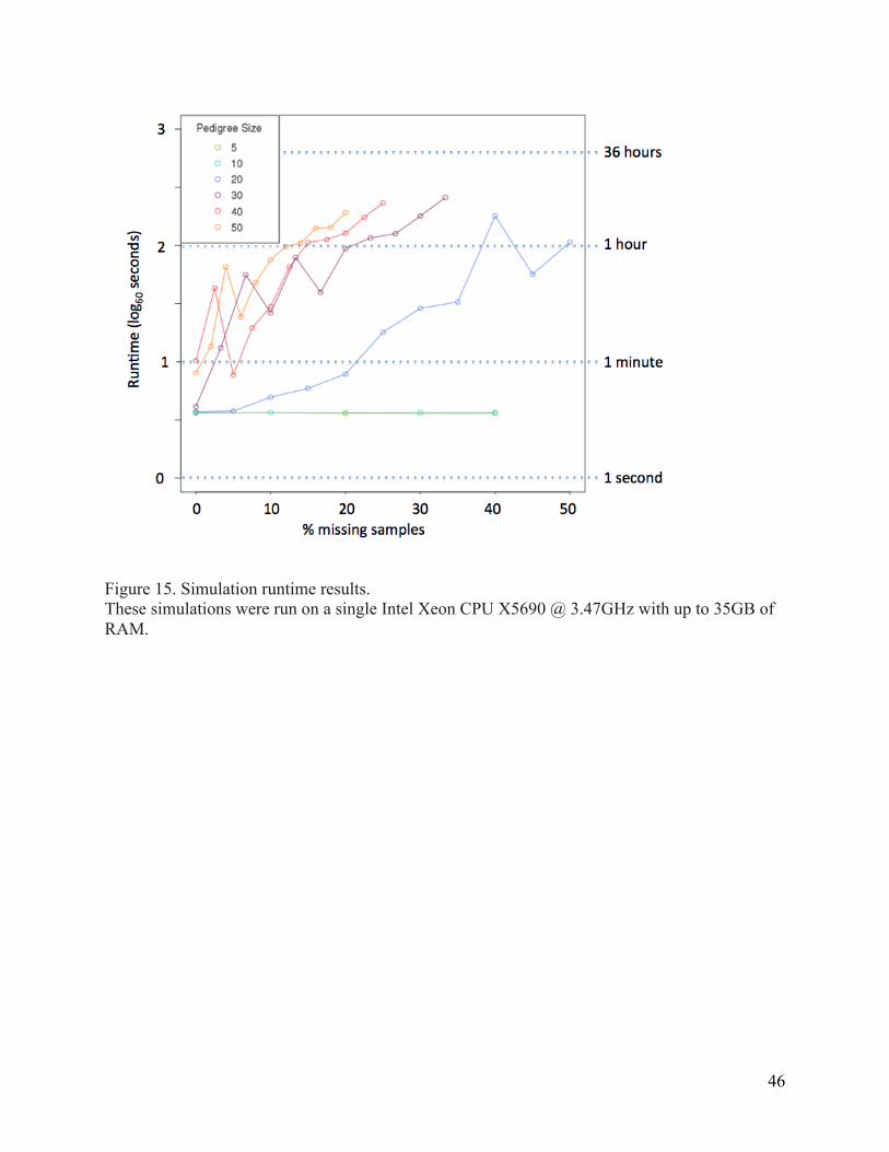
46
Figure 15. Simulation runtime results. These simulations were run on a single Intel Xeon CPU X5690 @ 3.47GHz with up to 35GB of RAM.

47
Figure 16. A pedigree correctly reconstructed by PRIMUS in nine seconds. PRIMUS used chip-based genotype data to verify this clinically ascertained pedigree, which included the presence of five individuals for whom no genetic data were available (individuals marked with diagonal lines) as well as a cycle in the pedigree generated by individual III-3 having children with both III-2 and III-4.
Figure 17. Two EOCOPD pedigrees verified by PRIMUS (A) This pedigree was the only pedigree generated from PRIMUS. (B) This pedigree was tied as the highest scoring pedigree with five other pedigrees.

48
Figure 18. Two of the six EOCOPD pedigrees corrected by PRIMUS. The reported pedigree is depicted above with the corrected pedigree below. Expected pedigree A has a non-paternity error so samples II-2 and II-3 are actually half-siblings rather than full-siblings in the correct pedigree (B). B was the top ranked pedigree in the PRIMUS output. Expected pedigree C contains not only a non-paternity that resulted in sample III-1 being a half-sibling to III-2 and III-3, but also a sample swap that resulted in sample II-3’s DNA being swapped for DNA of a sample in an entirely different pedigree. Corrected pedigree D was the only pedigree generated by PRIMUS. The investigators have independently confirmed the corrected pedigrees.

49
Using variant data obtained from exome sequencing generated by the UW CMG, PRIMUS
validated 49 pedigrees consisting of 351 individuals ascertained through a proband with severe
EOCOPD. The pedigrees range from size four with 50% missing samples to size 23 with 35%
missing samples. PRIMUS confirmed that 43 of the pedigrees matched the reported pedigrees
collected in the study. Among the remaining six pedigrees, PRIMUS found and corrected five
non-paternity errors, one sample swap, and one duplicate sample. These findings were consistent
with the corrections independently made by the Boston EOCOPD Study investigators who
compared estimates of IBDs obtained using PLINK with theoretical IBDs obtained using the
KINSHIP2 package (Web Resources). A summary of the EOCOPD reconstruction including
size, number of possible pedigrees, and where the true pedigree ranked in the possible pedigrees
is provided in Supplementary Table 4.
Figure 17 shows two reported pedigrees from the EOCOPD dataset that were verified by
PRIMUS. The pedigree depicted in Figure 17A was the only pedigree generated by PRIMUS
and the pedigree in Figure 17B was among the highest scoring pedigrees. Figure 18 shows two
of the reported pedigrees (A and C) that were corrected with PRIMUS (B and D). Figure 18A
had a non-paternity error so individuals A and B are actually half-siblings rather than full-
siblings (Figure 18B). For the reported pedigree in Figure 18C, PRIMUS not only corrected a
non-paternity revealing that individual B was a half-sibling to C and D, but also identified a
sample swap that resulted from A’s DNA being replaced with DNA from another individual in
the dataset. This corrected pedigree was the only pedigree generated by PRIMUS for these
samples.
Reconstructing and incorporating cryptic relatedness
To evaluate whether PRIMUS could incorporate cryptic relationships into known pedigrees, we
reconstructed pedigrees using the HapMap3 data72. Although the HapMap samples were
collected to contain trios, duos, and unrelated individuals, cryptic relatedness among these
samples is well established6, 19, 44. For example, the 10-person pedigree from individuals of
Mexican Ancestry in Los Angeles (MXL, Figure 19) has been manually reconstructed using
pairwise relationship predictions by several groups24; 44; 62.

50
We used PRIMUS to automatically reconstruct all pedigrees within each HapMap3 population,
and PRIMUS reconstructed cryptic pedigrees in nine of the eleven populations (Supplementary
Table 5). PRIMUS confirmed the relationships reported by the HapMap Consortium as well as
the cryptic 1st through 3rd degree relationships reported by Pemberton et al.44 and Kyriazopoulou-
Panagiotopoulou et al.24 (Supplementary Table 5). However, because PRIMUS uses all pairwise
relationships up to 3rd degree relatives to reconstruct the entire pedigree, it can consider each
relationship in the context of all others. This enabled our approach to correct one misspecified 1st
degree and two 2nd degree relationships reported by Pemberton et al. In addition to these
corrections, PRIMUS was able to increase the specificity of 13 2nd and 3rd degree relationship
predictions. For example, Pemberton et. al reported that MKK individuals NA21312 and
NA21370 had an unknown relationships status, but PRIMUS identified them as half-siblings.
PRIMUS eliminated all other 2nd degree relationships using the context of the other pairwise
relationships in the pedigree.
PRIMUS also identified 85 previously unreported24; 44 potential 3rd degree relationships among
the HapMap3 samples (Supplementary Table 5). Although we cannot be certain these
relationships are precise, our results provide strong evidence that relationships do exist and are
an improvement over the common assumption that these samples are unrelated. We have made
all reconstructed HapMap3 pedigrees available for download on the PRIMUS website (see Web
Resources).

51
Figure 19. A ten-person MapMap3 MXL pedigree obtained from the HapMap3 and 1000 Genomes samples. The pedigree includes three reported trios (each colored differently) from HapMap3 and an additional individual from the 1000 Genomes Project. The pedigree shown in A is one of four possible pedigrees that fit the estimated IBD proportions and is the pedigree previously reported24. Alternative possible pedigrees that fit the genetic data are shown in B, C, and D. For these MXL samples, PREPARE reported a single sibling relationship (NA19662, NA19685), the two first-cousin relationships (NA19662-NA19664 and NA19664-NA19685). PREPARE is presented to have automatically reconstructed the nine-person HapMap3 MXL pedigree reported in the CARROT paper24, but they only show that NA19686 (incorrectly labeled as NA19685 in Figure 14 of their paper60) and NA19665 are 2nd cousins. Unlike the PRIMUS automatic reconstruction (Figure 19), they do not show how the other eight individuals fit into the pedigree, nor do they acknowledge that there are four different pedigree structures that fit the genetic data.
52
Reconstruction of previously unknown pedigrees from Starr County
We used the Starr County Health Study to demonstrate the ability of PRIMUS to reconstruct
previously unknown pedigrees from a large genetic dataset. We calculated IBD estimates among
all 1,890 samples using genotypes obtained for the individuals (Affymetrix Genome-Wide SNP
Array 6.066). PRIMUS used these estimates to group 458 samples into 203 family networks of
two or more samples. Using only these genetic data, PRIMUS reconstructed a single possible
pedigree for 120 of these families in less than four minutes, and, based on our simulation results,
we expect that ~99.83% of these are the true pedigrees. When ages are provided to PRIMUS, it
flags pedigrees that are impossible given the ages of the samples (e.g., a parent being younger
than a child). Using the age information collected for the Starr County Heart Study dataset,
PRIMUS ruled out these incorrect pedigrees and identified a single possible pedigree for an
additional 73 families for a total of 193 novel pedigrees that range in size from two to five
individuals.
Comparing PRIMUS to competing methods
We compared the results of PRIMUS to those generated by RELPAIR, a program
commonly used to check relationships in genetic data. Using the method employed by
Pemberton et al.44, we compared the accuracy of the pairwise predictions of RELPAIR to the
accuracy of the pairwise relationships in the top ranked reconstructed pedigree produced by
PRIMUS (Figure 20 and Supplementary Table 3). Both methods had 100% accuracy when
distinguishing between 1st degree relationships; however, PRIMUS outperformed RELPAIR
when 2nd degree relationships were considered. While RELPAIR makes the distinction between
the 1st and 2nd degree relationships, it labels all third degree relationships as cousins. PRIMUS
distinguishes between the four 3rd degree relationships and also gives directionality to the
relationship (e.g., individual II-2 is the grandfather of individual IV-2 in Figure 16). Therefore,
to make a fair comparison between the ability of PRIMUS and RELPAIR to predict 3rd degree
relationships, we compared only the degree of the relationship predicted by PRIMUS to the
“cousin” prediction of RELPAIR. PRIMUS outperformed RELPAIR when classifying
relationships as 3rd degree, and as >3rd degree/unrelated (Figure 20; Supplementary Table 3).
53
We also compared PRIMUS to the latest pedigree reconstruction programs, PREPARE and
IPED2 (see Web Resources). Of the 9,717 simulated pedigrees of size ten to 50, only 43
pedigrees had all genotyped samples in a single generation, and all of these pedigrees had at least
one half-sibling relationship. Therefore, PREPARE and IPED2 could only attempt to correctly
reconstruct <0.5% of the simulated pedigrees; PRIMUS correctly reconstructed 9,008 of the
9,717 (92.7%) simulated pedigrees. Figure 21 shows PRIMUS reconstructions for additional
simple, common pedigree structures that PREPARE and IPED2 cannot completely reconstruct.
Additionally, neither PREPARE nor IPED2 can completely reconstruct any of the real data
presented in this manuscript because all of these pedigrees have genotyped samples from
multiple generations. PREPARE and IPED2 can provide a partial reconstruction by dropping
samples from higher generations and using only extant individuals, as the PREPARE authors did
with the MXL pedigree (Figure 14 of the PREPARE paper60; Figure 19). In order to reconstruct
relationships, PREPARE requires a priori information about which individuals are in the same
generation prior to reconstruction and cannot connect these pairwise relationships into a single,
multigenerational pedigree. PRIMUS completely reconstructs these pedigrees (e.g. Figure 19).
PREPARE and IPED2 provide limited utility to check reported pedigree structures and to
reconstruct previously unknown pedigrees de novo.
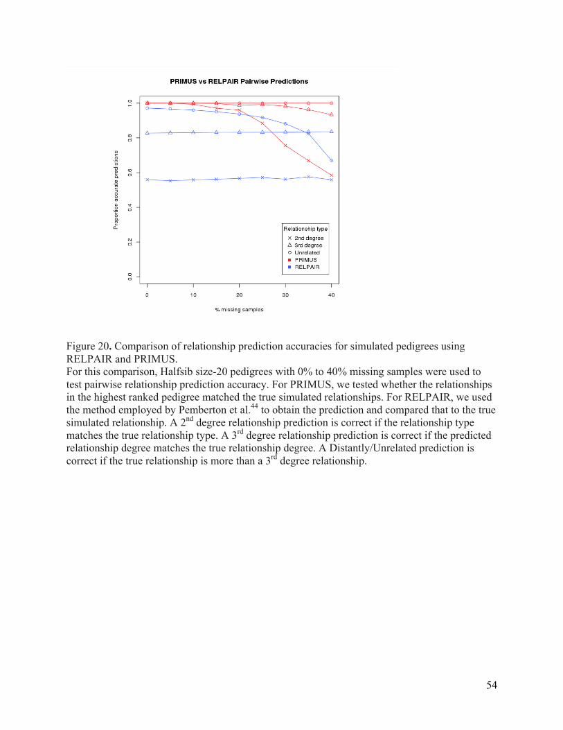
54
Figure 20. Comparison of relationship prediction accuracies for simulated pedigrees using RELPAIR and PRIMUS. For this comparison, Halfsib size-20 pedigrees with 0% to 40% missing samples were used to test pairwise relationship prediction accuracy. For PRIMUS, we tested whether the relationships in the highest ranked pedigree matched the true simulated relationships. For RELPAIR, we used the method employed by Pemberton et al.44 to obtain the prediction and compared that to the true simulated relationship. A 2nd degree relationship prediction is correct if the relationship type matches the true relationship type. A 3rd degree relationship prediction is correct if the predicted relationship degree matches the true relationship degree. A Distantly/Unrelated prediction is correct if the true relationship is more than a 3rd degree relationship.
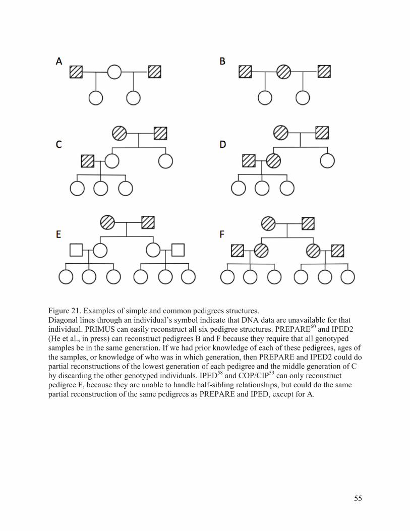
55
Figure 21. Examples of simple and common pedigrees structures. Diagonal lines through an individual’s symbol indicate that DNA data are unavailable for that individual. PRIMUS can easily reconstruct all six pedigree structures. PREPARE60 and IPED2 (He et al., in press) can reconstruct pedigrees B and F because they require that all genotyped samples be in the same generation. If we had prior knowledge of each of these pedigrees, ages of the samples, or knowledge of who was in which generation, then PREPARE and IPED2 could do partial reconstructions of the lowest generation of each pedigree and the middle generation of C by discarding the other genotyped individuals. IPED58 and COP/CIP59 can only reconstruct pedigree F, because they are unable to handle half-sibling relationships, but could do the same partial reconstruction of the same pedigrees as PREPARE and IPED, except for A.
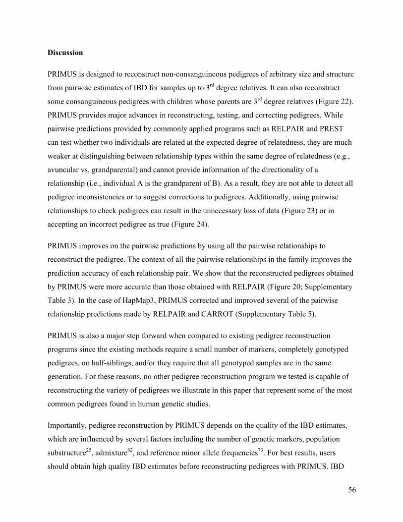
56
Discussion
PRIMUS is designed to reconstruct non-consanguineous pedigrees of arbitrary size and structure
from pairwise estimates of IBD for samples up to 3rd degree relatives. It can also reconstruct
some consanguineous pedigrees with children whose parents are 3rd degree relatives (Figure 22).
PRIMUS provides major advances in reconstructing, testing, and correcting pedigrees. While
pairwise predictions provided by commonly applied programs such as RELPAIR and PREST
can test whether two individuals are related at the expected degree of relatedness, they are much
weaker at distinguishing between relationship types within the same degree of relatedness (e.g.,
avuncular vs. grandparental) and cannot provide information of the directionality of a
relationship (i.e., individual A is the grandparent of B). As a result, they are not able to detect all
pedigree inconsistencies or to suggest corrections to pedigrees. Additionally, using pairwise
relationships to check pedigrees can result in the unnecessary loss of data (Figure 23) or in
accepting an incorrect pedigree as true (Figure 24).
PRIMUS improves on the pairwise predictions by using all the pairwise relationships to
reconstruct the pedigree. The context of all the pairwise relationships in the family improves the
prediction accuracy of each relationship pair. We show that the reconstructed pedigrees obtained
by PRIMUS were more accurate than those obtained with RELPAIR (Figure 20; Supplementary
Table 3). In the case of HapMap3, PRIMUS corrected and improved several of the pairwise
relationship predictions made by RELPAIR and CARROT (Supplementary Table 5).
PRIMUS is also a major step forward when compared to existing pedigree reconstruction
programs since the existing methods require a small number of markers, completely genotyped
pedigrees, no half-siblings, and/or they require that all genotyped samples are in the same
generation. For these reasons, no other pedigree reconstruction program we tested is capable of
reconstructing the variety of pedigrees we illustrate in this paper that represent some of the most
common pedigrees found in human genetic studies.
Importantly, pedigree reconstruction by PRIMUS depends on the quality of the IBD estimates,
which are influenced by several factors including the number of genetic markers, population
substructure25, admixture62, and reference minor allele frequencies73. For best results, users
should obtain high quality IBD estimates before reconstructing pedigrees with PRIMUS. IBD

57
estimates can be obtained by PRIMUS or by another program (PLINK23, KING25, or REAP62)
that uses the appropriate allele frequencies for the ancestry of the samples and accounts for
potential admixture and population substructure among the data.
We designed PRIMUS to reconstruct up to 3rd degree relationships for several reasons. First, the
distance between the expected mean genome-wide IBD proportions for more distant
relationships (e.g., 4th degree and 5th degree) is small while the variation around these means is
large. Therefore, the overlap between the distributions of these distant relationships precludes
highly accurate relationship assignments of any relationship beyond 3rd degree. Second, as the
relationship distance increases beyond 3rd degree, the number of possible relationships increases
rapidly (Supplementary Table 6), and pedigree reconstruction quickly becomes computationally
challenging. For more distant relationships, it is possible to apply programs such as BEAGLE42
and ERSA27 to connect the sub-pedigrees obtained by PRIMUS that are distantly related to one
another, and we have incorporated this feature in a follow-up release of PRIMUS described in
Chapter 5. Additionally, programs like RELPAIR28 could improve the pairwise relationship
prediction because they model recombination events to distinguish between 2nd degree
relationships. The improved relationship predictions could then be used to improve the scoring of
possible pedigrees.
We have identified two limitations of PRIMUS and their corresponding remedies. First, due to
computational restraints, PRIMUS was unable to complete the reconstruction of 6.3% of
simulations using 3rd degree relatives or closer. The vast majority of these pedigrees had ≥30
individuals with >20% missing sample data. Investigators can still greatly benefit from partial
reconstructions of these pedigrees. Users can obtain a partial reconstruction, as we did, by using
a higher relatedness threshold to reconstruct using just 1st or 2nd degree relationships. Second, for
a very small proportion of the simulations (~0.5%), PRIMUS did not output the true pedigree
among the results because the initial likelihood threshold was set too high. Yet by lowering the
initial likelihood threshold used to predict familial relationships, PRIMUS was able to
reconstruct each of these pedigree structures. Therefore, for a very small percentage of pedigrees
run on PRIMUS, it may be necessary to depart from the default initial likelihood threshold to
obtain a reported pedigree.

58
PRIMUS provides an immediate benefit to the genetics community in two ways: pedigree
verification and pedigree discovery. Because PRIMUS computationally verifies reported
pedigrees using genotype data and identifies and corrects inconsistencies, PRIMUS saves a
significant amount of time and effort that would otherwise be spent on manual verification of
pedigrees. This is especially beneficial when large, complex pedigrees are being studied similar
to the Boston EOCOPD Study pedigrees. For example, PRIMUS has identified and corrected
non-paternities, under-related samples, samples swaps, duplicate samples, and unexpected
consanguinity in clinical pedigrees (Figure 19 and Figure 20). In many cases, such corrections
can result in a correction of the genetic model and assumptions used for downstream analysis,
improving the chances of finding the genetic cause of the disease.
Moreover, PRIMUS can reconstruct previously unknown pedigrees using only genetic data, as
demonstrated in the HapMap3 and Starr County datasets. Although, PRIMUS cannot guarantee
that these pedigrees are the true pedigrees, the pedigrees can be treated as a hypothesis to be
confirmed with supporting independent evidence. This application of PRIMUS is particularly
useful in large-scale genetic studies where substantial cryptic relatedness may exist. In the case
of the Starr County data, we can now use powerful family-based analyses that leverage the
information contained in nearly 200 previously unknown pedigrees.
Incomplete understanding of relatedness structures (i.e., pedigrees) within genetic data can result
in a vast array of analytic problems, from dramatically biased effects of rare variants to power
loss in pedigree-based methods. With the introduction of PRIMUS, we hope to address many of
the limitations of prior pedigree reconstruction frameworks and pairwise comparison algorithms
in a fast, tractable, and easy to use algorithm, enabling investigators to better assess the
information present within their data.
59
Figure 22. A pedigree from the University of Washington Center for Mendelian Genomics. The parents were reported as unrelated individuals by the clinician as depicted in pedigree A, but PRIMUS reconstructed them as first cousins, as depicted in pedigree B.

60
Figure 23. An example where pairwise relationship checking and removal of an inconsistent sample results in an analysis loss. Panel A shows the reported pedigree as provided by the investigator. Pairwise relationship checking reveals that all relationships are correct except between sample II-5 and the siblings III-1 and III-2. Standard practice is to remove inconsistent samples, in this case sample II-5, resulting in the 5-person pedigree on the right. Panel B shows the true pedigree where sample II-5 was actually the father of the siblings III-1 and III-2 instead of individual II-2, who was not successfully genotyped, being the father. The mix-up could realistically be explained by a sample swap or by misspecified paternity for the two children, and these types of errors are common. Pedigree reconstruction would have revealed the inconsistency and would have easily reconstructed the true pedigree. Therefore, rather than discarding 17% of the data, the investigator could have retained all samples.

61
Figure 24. An example where pairwise relationship checking and removal of an inconsistent samples results in an unnecessary data loss and the use of an incorrect pedigree. Panel A shows the pedigree as reported by the investigator. Pairwise relationship checking reveals that all relationships are correct except between sample I-1 and samples III-1, IV-1, and IV-2. Standard practice is to remove inconsistent samples, in this case sample I-1, resulting in the 4-person pedigree on the right. Panel B shows the true pedigree. The error in the original pedigree was that sample II-1 was incorrectly assigned as the uncle to sample III-1, when, in fact, they were half-siblings. This mix-up could realistically be explained if the family incorrectly reported their family history or by a clerical error, and these types of errors are common. Pedigree reconstruction would easily have revealed the inconsistency and would have reconstructed the true pedigree. Therefore, rather than discarding 20% of the data and assuming an incorrect pedigree, the investigator would have retained all samples and used the true pedigree in further analyses.

62
Chapter 4. Incorporating mtDNA and NRY Haplotypes into pedigree
reconstruction
PRIMUS is a pedigree reconstruction algorithm that uses estimates of genome-wide identity by
descent to reconstruct pedigrees consistent with the observed genetic data. However, when the
genetic data for a set of individuals within a pedigree are missing, multiple pedigrees can be
reconstructed. We report a major expansion of PRIMUS that uses mitochondrial (mtDNA) and
non-recombining Y chromosome (NRY) haplotypes to eliminate many of the pedigree structures
that are inconsistent with the genetic data. We demonstrate that discordances in mtDNA and
NRY haplotypes substantially reduce the number of potential pedigrees, and can often lead to the
identification of the correct pedigree.
Introduction
Correctly determining pedigree structures is key to identifying the causes of genetic disorders2-6;
9. In some cases, reported pedigree structures are inconsistent with the samples20-22, resulting in a
loss of power that could result in failure to find a disease causing variant19. Unexpected
relationships among samples in large genetic datasets are also common. Cryptic relatedness
within datasets or between pedigrees, as well as sample swaps, is frequently observed. Pedigree
reconstruction can find cryptic relationships and correctly fit them into a pedigree structure74.
Early methods for checking pedigrees applied pairwise comparison methods28; 29; however,
pedigree reconstruction can more accurately predict relationships, find the correct pedigree, and
identify cryptic pedigrees within the data74. PRIMUS uses estimates of genome-wide identity by
descent (IBD) to identify families and reconstruct all possible pedigrees that fit the IBD
estimates up to 3rd degree relationships.
Missing genetic data for a set of people in a family can often lead to the identification of multiple
pedigrees that fit the genetic data. We show that using inconsistencies in the inheritance patterns
of mitochondrial DNA (mtDNA) and non-recombining Y chromosome (NRY) haplotypes,
which are captured by genotyping arrays or by high-throughput sequencing 75, improves the
accuracy of pedigree reconstruction. We have developed a new module for the pedigree

63
reconstruction in PRIMUS (v1.8.0) that utilizes mtDNA and NRY data to reduce the number of
possible pedigrees and improve the chance of identifying the correct pedigree structure.
Methods
Identifying concordant and discordant mtDNA and NRY haplotypes
PRIMUS supports standard, easy-to-use formats that now include data with mtDNA and NRY
haplotypes. NRY and mtDNA can be encoded as chromosome 24 and 26, respectively, in a
PLINK-formatted data file or in any other format accepted by PLINK. For a pair of individuals,
PRIMUS calculates the concordance of mtDNA and NRY haplotypes. The percent concordance
of a haplotype is calculated as the percentage of matching mtDNA and NRY nucleotide positions
across the total number of variable mtDNA and NRY positions and excludes positions with
missing calls. A “discordant” prediction between the NRY or mtDNA haplotype of two
individuals occurs when concordance is below a user definable cutoff (default is 99%);
otherwise, the NRY or mtDNA haplotype is predicted to be “concordant.” The discordant status
indicates that a pair of individuals has not inherited the mtDNA or NRY haplotypes from a
recent common ancestor. Therefore, PRIMUS can eliminate any pedigree structure where a pair
of individuals has discordant mtDNA or NRY haplotypes.
By default, PRIMUS only eliminates pedigree structures that are inconsistent with the discordant
predictions of mtDNA and NRY, which we demonstrate are very informative and reliable. For
example, in both sequencing and genotyping datasets, we observed a nearly 100% haplotype
concordance between individuals who have inherited mtDNA or NRY from a recent common
ancestor (i.e., fewer than four generations of separation; Table 5); therefore, individuals with
discordant predictions are very unlikely to be related to a recent common ancestor of the sex that
corresponds to the discordant mtDNA or NRY prediction.
Although discordant mtDNA and NRY haplotypes are very useful in rejecting genetically
inconsistent pedigrees, concordant haplotypes are less so. Because recombination does not
influence mtDNA and NRY haplotypes, a single haplotype can be passed unchanged through a
family for generations. Therefore, distant relatives can have concordant mtDNA and NRY
haplotypes while they share little or no autosomal-DNA with detectable IBD (Figure 25). If
64
PRIMUS requires all concordant mtDNA and NRY predictions to be represented by a recent
common ancestor, then distant, concordant ancestral mtDNA and NRY haplotypes can cause
PRIMUS to reject the correct pedigree structure. Therefore, by default concordant mtDNA and
NRY haplotypes are not used to rule out pedigree structures.
mtDNA and NRY checking
PRIMUS uses mtDNA and NRY discordance to improve pedigree reconstructions by checking
whether the discordance is consistent with the expected mtDNA and NRY inheritance patterns
within the pedigree. For example, if half-siblings are genotyped and have discordant mtDNA
prediction, then their parent in common must be the father. To check whether this discordant
prediction is consistent with a pedigree structure, PRIMUS finds the shortest first-degree-relative
inheritance path connecting two individuals, A and B. Discordant predictions require an
interruption in the transmission of the haplotype in the pedigree. For example, if A and B have a
discordant NRY prediction, then there must be a female somewhere in the NRY inheritance path.
The logic that applies to NRY inheritance paths through males also applies to mtDNA
inheritance paths through females, except that the sex of A and B does not matter unless one is
the direct ancestor of the other; in which case, the direct ancestor must be female. We illustrate
valid and invalid inheritance paths within a pedigree in Figure 26.
Results
We modified the pedigree simulations described in Staples et al. 74, to explore the affects of
using mtDNA and NRY during reconstruction of pedigrees with different structures, genotypes
and combinations of missing samples. We selected pedigrees of size 20 and masked the
genotypes for 0-50% of individuals in the pedigree. We modified the simulations by permuting
the sex of the individuals, while maintaining the biological integrity of the pedigree. For each
simulation, we assigned a unique NRY haplotype to each male founder and a unique mtDNA
haplotype to all founders and propagated these genotypes through the pedigree. We ascertained
mtDNA and NRY haplotypes from the phase 1 release of unrelated CEU and TSI haplotypes 18
with individual-level call rates >90% from the 1000 Genomes Project 51. The haplotypes
consisted of 2,832 mtDNA and 8,665 NRY variants with quality score ≥30 and call rates >95%,
and with a minor allele frequency >1% for inclusion.

65
We considered pedigree reconstruction performance on the autosomal data alone as the baseline
and compared this to the performance when we added additional information such as sex status,
mtDNA and NRY. We see a moderate reduction in the number of possible pedigrees with
mtDNA and NRY individually, but the synergistic effects of mtDNA and NRY with sex status
exceeded the combined individual improvements (Figure 27). Our results show the largest
improvement in pedigrees with more missing samples (35-40%) where a 37% reduction in the
mean number of genetically consistent pedigrees is seen (Figure 27). The improvement declines
beyond 40% missing samples because the pedigrees become too sparse for the discordant
mtDNA and NRY haplotypes to rule out possible pedigrees. We also see a substantial
improvement in ranking the correct pedigree structure (Figure 28). In fact, when mtDNA and
NRY are combined with individual sex status, we see a 4.5-fold increase over sex status alone in
the number of simulations that reconstructed to only the true pedigree (Figure 28).
The improvements in pedigree specificity using mtDNA and NRY genotypes are remarkable. As
shown in Figure 29, a dataset that reconstructed to 58 possible pedigrees using autosomal DNA
and sex status resolved to the single correct pedigree with the addition of mtDNA data. The new
implementation of PRIMUS identified this pedigree by eliminating the 57 pedigrees that were
inconsistent with the mtDNA data. NRY and mtDNA provide a substantial improvement in
automated pedigree reconstruction with PRIMUS.

66
Figure 25. Summary of the haplotype discordance between pairs of individuals. Panel A and B show the haplotype discordance for the low-pass 1000 Genomes Project 51 phase 1 release using 2,832 high quality mtDNA sites and 8,665 high quality NRY sites from 548 females and 526 males. Panel C and D show haplotype discordance for 372 individuals genotyped with the Illumina Infinium HumanCoreExome-24 BeadChips (HCE) array for 205 high quality mtDNA sites and 126 high quality NRY sites genotyped in 185 female and 187 male samples. (A) Of the ~576,000 mtDNA pairwise comparisons, 99.5% are more than 0.1% discordant; however, 2,684 pairs of individuals have haplotypes that are >99.9% identical. The majority of these pairs are in individuals that are more distantly related than 3rd degree relatives. (B) All male/male NRY chromosome comparisons in 1000 Genomes. (C) ~69,000 pairwise comparisons between 372 individuals from HCE dataset. (D) All male/male NRY chromosome comparisons in HCE dataset.

67
Figure 26. Examples of (A) mtDNA and (B) NRY inheritance paths in a pedigree. Individuals who share identical mtDNA or NRY haplotypes have the same symbol color. Diagonal lines through the symbol indicate that there was no genetic data available for the individual; therefore, sex of those individuals cannot be determined prior to reconstruction with mtDNA and NRY data. The dotted lines passing through multiple individuals represent examples of possible inheritance paths for mtDNA and NRY. (A) mtDNA is passed from mother to child. Path 1 shows a valid mtDNA inheritance path that passes from a grandmother to her grandson through the grandson’s mother. If the grandmother’s and grandson’s mtDNA were discordant, then PRIMUS would reject this pedigree because it is inconsistent with a mtDNA inheritance path. Path 2 shows an invalid mtDNA inheritance that passes through a male where the grandmother and granddaughter have discordant mtDNA haplotypes. Path 3 shows an invalid mtDNA inheritance path because the most recent ancestral person in the path is male. (B) Path 1 shows a valid NRY inheritance path where the males at the end of the path have concordant predictions; if not, then this pedigree would be inconsistent with the NRY haplotypes, and it would be rejected. Path 2 shows an invalid NRY inheritance path for the two males because the grandson could not inherit the grandfather’s NRY through the mother.

68
Figure 27. A summary of the percent reduction in the average number of possible pedigrees when data from mtDNA haplotypes, NRY halpotypes, sex or all of these are applied in pedigree analysis. The addition of either mtDNA or NRY data outperforms the addition of only sex status. The greatest reduction in the number of possible pedigrees is obtained when mtDNA, NRY and sex status are combined, eliminating nearly 40% of the incorrect pedigrees.

69
Figure 28. Relative improvement of reconstruction of simulated pedigrees with 35% masked samples with additional data (i.e., sex status, NRY and mtDNA haplotypes). The ideal would be to reconstruct as few pedigrees as possible while retaining the correct pedigree, and to rank the correct pedigree as the highest when multiple pedigrees are consistent with the genetic data. When the correct pedigree is not the highest rank, or tied to the highest rank pedigree, the addition of mtDNA and mtDNA + NRY + Sex provides a substantial improvement in the number of pedigrees that become the highest ranked or only pedigree by eliminating pedigrees that are not compatible with the observed mtDNA, or mtDNA and NRY haplotypes and Sex.
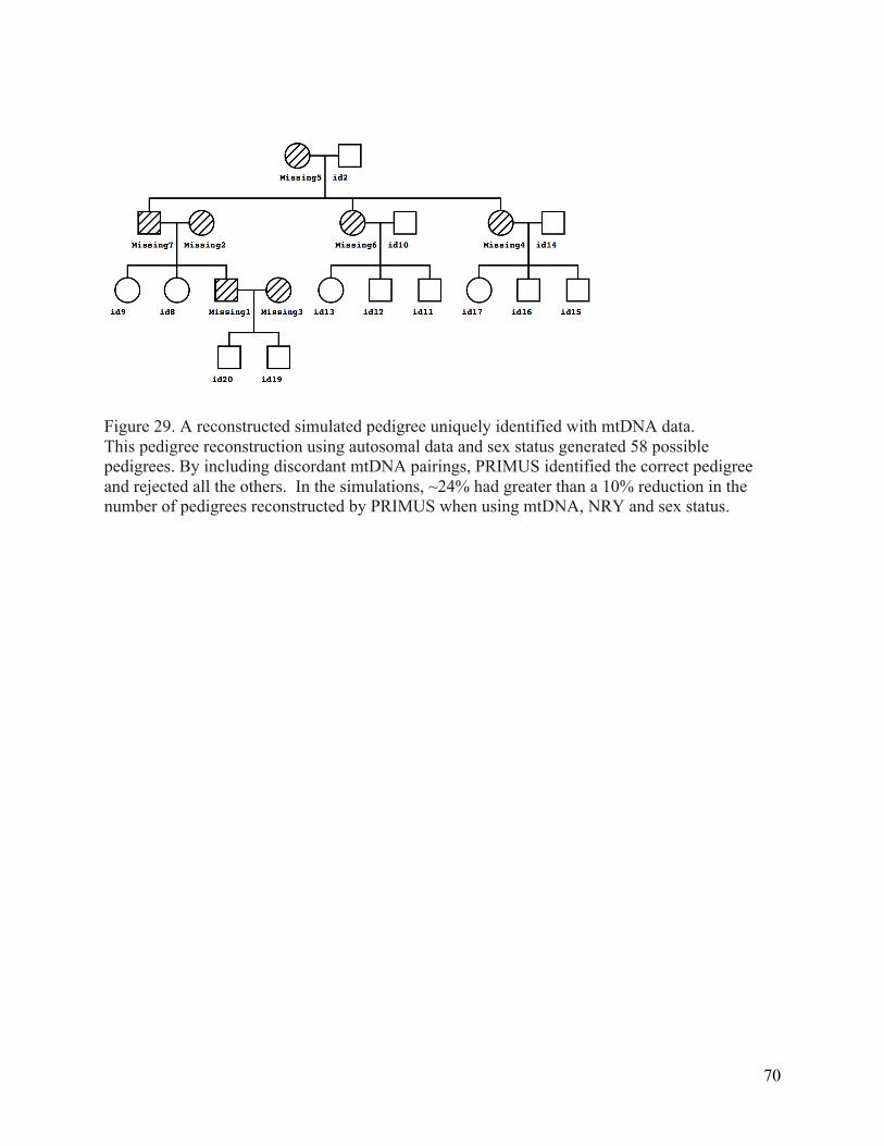
70
Figure 29. A reconstructed simulated pedigree uniquely identified with mtDNA data. This pedigree reconstruction using autosomal data and sex status generated 58 possible pedigrees. By including discordant mtDNA pairings, PRIMUS identified the correct pedigree and rejected all the others. In the simulations, ~24% had greater than a 10% reduction in the number of pedigrees reconstructed by PRIMUS when using mtDNA, NRY and sex status.

71
Table 5. A summary of the concordance between pairs of individuals known to have concordant mtDNA or NRY haplotypes.
# of pairs
% of pairs 100%
concordant
% of pairs >99.8%
concordance
A. 1KG mtDNA mother/child and full-‐siblings 21 62% 100%
B. 1KG NRY father/son and male full-‐siblings 5 40% 100%
C. HCE mtDNA mother/child and full-‐siblings 67 100% 100%
D. HCE NRY father/son and make full-‐siblings 23 100% 100%
Summary of the sequence identity between pairs of individuals from the low-pass 1000 Genomes Project 51 phase 1 release (A and B) and from 372 individuals with Illumina Infinium HumanCoreExome-24 BeadChips (HCE) chip data (C and D). We used 2,832 high quality mtDNA sites and 8,665 high quality NRY sites from the 1000 Genomes Project. The HCE data contain 205 high quality mtDNA sites and 126 high quality NRY sites from 185 female and 187 male samples. Every pairwise relationship included in the figures is expected to be nearly identical since they were either directly passed from an individual to the other or both inherited mtDNA or NRY from mother and dad, respectively. (A) 1000 Genomes mother/child and siblings have the same mtDNA DNA and should, therefore, have very few, if any, differences in the mtDNA sequence. These results show that there is less than 0.2% sequence difference between these pairs of individuals. (B) 1000 Genomes Father/son comparison; there are less than 0.2% sequence difference among these pairs. (C). HCE Mother/child or full-sibling pairs have 100% mtDNA genotype identity. (D) HCE Father/child and male full-sibling pairs have 100% NRY genotype identity.
72
Chapter 5. PADRE: Pedigree Aware Distant Relationship Prediction
Accurate estimation of shared ancestry is important in genetics studies. Current relationship
prediction programs have the ability to accurately estimate pairwise relationships as distant as
ninth-degree relatives. We demonstrate that combining distant relationship estimates with
pedigree reconstruction can provide improved accuracy and power to estimate more distant
relationships (i.e., more than ninth-degree relatives) depending on the depth of the pedigrees. We
have developed a Pedigree Aware Distant Relationship Estimation (PADRE) algorithm that uses
relationship likelihoods generated by Estimation of Recent Shared Ancestry (ERSA) to identify
the highest likelihood connection between family networks reconstructed by PRIMUS (Pedigree
Reconstruction and Identification of a Maximum Unrelated Set). We used PADRE to estimate
relationships from SNP genotypes for both simulated pedigrees and 169 individuals from three
previously described extended pedigrees. PADRE provides a substantial improvement in both
the accuracy and power to detect distant relationships compared to ERSA alone, by correctly
predicting 20% more of the fourth- through ninth-degree simulated relationships within one
degree. PADRE also correctly predicts 59% of the tenth- through thirteenth-degree simulated
relationships within one degree of relatedness, compared to 4% with ERSA alone. The
improvement seen in the real pedigrees is broadly consistent with the improvement seen in
simulations. We also used PADRE to estimate the distant relationships among the HapMap3
CEU samples, illustrating how the different trios and individuals are interconnected. PADRE
greatly expands the range of relationships that can be estimated from genetic data that contain
pedigrees and, it is implemented in the PRIMUS software package.
Introduction
Accurate prediction and verification of relationships among individuals is essential in a variety
of genetic studies. Errors in pedigrees are common20-22 and have adverse consequences,
including a drop in the power to detect linkage19. Therefore, ensuring that the genetic
relationships among the DNA samples match the reported pedigree structure is critical and
improve linkage analysis and other forms of genetic analysis74. Identifying cryptic relationships
can be useful as well. Genetic relationships identified in population studies can be also leveraged

73
for improved phasing and imputation. The identification of relatives also plays an important role
in forensics in criminal investigations76 and with victims of mass disaster77.
With close relationships (first- through third-degree), pedigree reconstruction can provide the
structure of the individuals in a genetic dataset74. However, genetic datasets often contain
relationships that are more distant than third-degree, resulting in sparsely connected pedigrees
that are unsuitable for reconstruction. Segmental sharing algorithms, such as ERSA27; 38, can
accurately predict pairwise relationships up to ninth-degree relatives (third-cousins once
removed), but do not reconstruct pedigrees nor can they utilize information from known or
observed pedigree structures in the data. We report the development of a new algorithm that
leverages the pedigree reconstruction of first- to third-degree relatives by PRIMUS74 with the
accurate distant relationship predictions by ERSA38, known as PADRE (Pedigree Aware Distant
Relationship Estimation), which we have implemented in PRIMUS. PADRE uses ERSA-
generated relationship likelihoods to identify the highest likelihood connection between family
networks reconstructed by PRIMUS, which significantly expands the relationships that can be
predicted.
Methods
Pedigree Aware Distant Relationship Estimation (PADRE) algorithm
PADRE combines reconstructed pedigree information with distant pairwise relationship
predictions to determine the most likely way that two pedigrees may be distantly related. The
algorithm is implemented within PRIMUS (v1.8.0) and requires results from ERSA (v2.1) as
input. When PRIMUS reconstructs a dataset into two family networks, Net1 and Net2, both
networks can have one or more possible pedigrees that fit the genetic data, annotated here with
subscripts (i.e., Net11, Net12,…, and Net1n).
The ERSA pairwise relationship model has two additional degree of freedom (relationship
distance and number of shared segments) compared to the model that specifies two individuals
are unrelated. Therefore, PADRE uses the Akaike Information Criterion (AIC) to penalize the
related ERSA model for having two additional degrees of freedom. For a statistical model, the
AIC value is 𝐴𝐼𝐶 = 2k− 2𝑙𝑛𝑙 𝐿 , where k is the number of parameter in the model and L is the
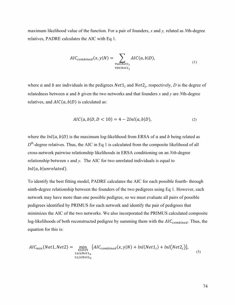
74
maximum likelihood value of the function. For a pair of founders, x and y, related as Nth-degree
relatives, PADRE calculates the AIC with Eq 1.
𝐴𝐼𝐶!"#$%&'( 𝑥,𝑦 𝑁 = 𝐴𝐼𝐶 𝑎, 𝑏 𝐷 ,∀!∈!"#!!∀!∈!"#!!
(1)
where 𝑎 and 𝑏 are individuals in the pedigrees 𝑁𝑒𝑡1! and 𝑁𝑒𝑡2!, respectively, D is the degree of
relatedness between 𝑎 and 𝑏 given the two networks and that founders x and y are Nth-degree
relatives, and 𝐴𝐼𝐶 𝑎, 𝑏 𝐷 is calculated as:
𝐴𝐼𝐶 𝑎, 𝑏 𝐷,𝐷 < 10 = 4− 2𝑙𝑛𝑙 𝑎, 𝑏 𝐷 , (2)
where the 𝑙𝑛𝑙 𝑎, 𝑏 𝐷 is the maximum log-likelihood from ERSA of 𝑎 and 𝑏 being related as
Dth-degree relatives. Thus, the AIC in Eq 1 is calculated from the composite likelihood of all
cross-network pairwise relationship likelihoods in ERSA conditioning on an Nth-degree
relationship between x and y. The AIC for two unrelated individuals is equal to
𝑙𝑛𝑙 𝑎, 𝑏 𝑢𝑛𝑟𝑒𝑙𝑎𝑡𝑒𝑑 .
To identify the best fitting model, PADRE calculates the AIC for each possible fourth- through
ninth-degree relationship between the founders of the two pedigrees using Eq 1. However, each
network may have more than one possible pedigree, so we must evaluate all pairs of possible
pedigrees identified by PRIMUS for each network and identify the pair of pedigrees that
minimizes the AIC of the two networks. We also incorporated the PRIMUS calculated composite
log-likelihoods of both reconstructed pedigree by summing them with the 𝐴𝐼𝐶!"#$%&'(. Thus, the
equation for this is:
𝐴𝐼𝐶!"# 𝑁𝑒𝑡1,𝑁𝑒𝑡2 = min!!!!!
!!!!!"#!!!!!!!"!!!
𝐴𝐼𝐶!"#$%&'( 𝑥,𝑦 𝑁 + 𝑙𝑛𝑙 𝑁𝑒𝑡1! + 𝑙𝑛𝑙 𝑁𝑒𝑡2! , (3)
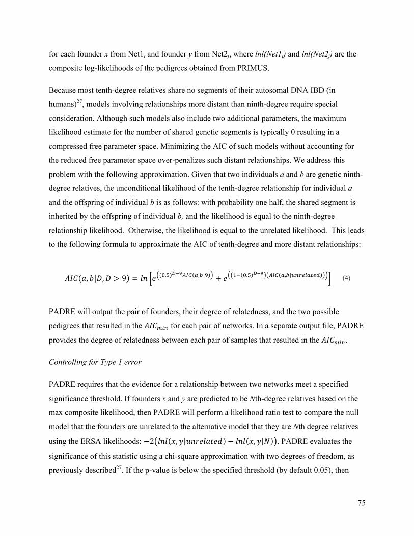
75
for each founder x from Net1i and founder y from Net2j, where lnl(Net1i) and lnl(Net2j) are the
composite log-likelihoods of the pedigrees obtained from PRIMUS.
Because most tenth-degree relatives share no segments of their autosomal DNA IBD (in
humans)27, models involving relationships more distant than ninth-degree require special
consideration. Although such models also include two additional parameters, the maximum
likelihood estimate for the number of shared genetic segments is typically 0 resulting in a
compressed free parameter space. Minimizing the AIC of such models without accounting for
the reduced free parameter space over-penalizes such distant relationships. We address this
problem with the following approximation. Given that two individuals a and b are genetic ninth-
degree relatives, the unconditional likelihood of the tenth-degree relationship for individual a
and the offspring of individual b is as follows: with probability one half, the shared segment is
inherited by the offspring of individual b, and the likelihood is equal to the ninth-degree
relationship likelihood. Otherwise, the likelihood is equal to the unrelated likelihood. This leads
to the following formula to approximate the AIC of tenth-degree and more distant relationships:
𝐴𝐼𝐶 𝑎, 𝑏 𝐷,𝐷 > 9 = 𝑙𝑛 𝑒 (!.!)!!!!"# !,! ! + 𝑒 !! !.! !!! !"# !,! !!"#$%&#' (4)
PADRE will output the pair of founders, their degree of relatedness, and the two possible
pedigrees that resulted in the 𝐴𝐼𝐶!"# for each pair of networks. In a separate output file, PADRE
provides the degree of relatedness between each pair of samples that resulted in the 𝐴𝐼𝐶!"#.
Controlling for Type 1 error
PADRE requires that the evidence for a relationship between two networks meet a specified
significance threshold. If founders x and y are predicted to be Nth-degree relatives based on the
max composite likelihood, then PADRE will perform a likelihood ratio test to compare the null
model that the founders are unrelated to the alternative model that they are Nth degree relatives
using the ERSA likelihoods: −2 𝑙𝑛𝑙 𝑥,𝑦 𝑢𝑛𝑟𝑒𝑙𝑎𝑡𝑒𝑑 − 𝑙𝑛𝑙 𝑥,𝑦 𝑁 . PADRE evaluates the
significance of this statistic using a chi-square approximation with two degrees of freedom, as
previously described27. If the p-value is below the specified threshold (by default 0.05), then

76
PADRE includes the relationship between the pair of networks in the results. For the CEU
pedigrees, we applied a Bonferroni correction of p = 5.5x10⁻⁶ (0.05 / 9074 founder-to-founder
relationships) to account for the number of founder-to-founder relationships tested in the CEU
pedigree reconstruction results.
Simulations
We simulated pedigrees to evaluate the accuracy and relative benefit of using PADRE to detect
distant relationships compared to ERSA alone. We used two identical 13-person, 3-generation
pedigree structures and connected a founder in each pedigree by varying the number of
generations to their recent common ancestor. Figure 30 illustrates a simulated pedigree where
founders A2 and B2 are ninth-degree relatives. To test the full range of ERSA predictions
beyond third-degree, we generated versions of the pedigree where individuals A2 and B2 are
fourth- through ninth-degree relatives. For each of these versions of simulated pedigree
structures, we created 100 different sets of genotypes using the method applied by Morrison61
(see Web Resources). We randomly selected haplotypes with ~1M SNPs from among the
unrelated HapMap372 CEU samples and assigned them to the two founders and anyone who
married into the simulated pedigrees. The unrelated set of CEU samples was determined by
running ERSA on all the HapMap3 CEU samples and then running the IMUS algorithm within
PRIMUS18 to identify the maximum unrelated set. We then propagated the genotypes from the
founders through the pedigree by simulating recombination events as a homogeneous Poisson
process using the genetic map provided with the HapMap3 data, but disregarding the centromere.
Genotypes were removed for all individuals not included in either of the 13-person pedigrees.
IBD estimates were calculated using PLINKv1.9, and all simulated pedigrees were reconstructed
with PRIMUS. We obtained ERSA results as described above for each simulation.
To test improvements in relationship predictions by PADRE as the size and density of genotyped
individuals increased, we first used PRIMUS, ERSA, and PADRE to analyze individuals A6 and
B6 in each simulated pedigree (Figure 30). We then included genotypes of a randomly selected
first- or second-degree relative of A6 and B6 and reran the analysis and comparison. We
repeated this process until all first- and second-degree relatives of A6 and B6 were included,
which results in two 10-person pedigrees connected by a single fourth- through ninth degree

77
relationship between A2 and B2. We then performed a final analysis and comparison using all 13
individuals in each pedigree.
Extended Pedigree Samples
We analyzed Affymetrix 6.0 SNP microarray data on 169 individuals from three previously
described extended pedigrees with predominantly northern European ancestry (Huff,
Witherspoon, et al., 2010). The three pedigrees were composed of 24, 30, and 115 genotyped
individuals and included a total of 7,266 pairs of related individuals.
HapMap3 CEU samples
Using 165 CEU individuals from HapMap3 release 272 obtained from
http://hapmap.ncbi.nlm.nih.gov, we reconstructed pedigree structures within this dataset using
PRIMUS as described below using the default settings. We also ran ERSA on the dataset as
described above, using the CEU dataset as its own control file to identify the regions for
masking38.
Pedigree reconstruction with PRIMUS
PRIMUS reconstructs multiple generation pedigrees with genotyped individuals in any
generation74. PRIMUS uses genome-wide identity by descent (IBD) estimates to identify
families and reconstruct all possible pedigrees that fit the genetic data using relationships as
distant as third-degree relatives. We used the prePRIMUS IBD pipeline74 to generate IBD
estimates between all samples in each pedigree and PRIMUS to reconstruct pedigrees. Due to the
sparse number of individuals genotyped in the three European ancestry pedigrees and in many of
the simulations, we applied a relatedness cutoff in PRIMUS of second-degree to both datasets.
We used the default relatedness cutoff of third-degree relatives for the HapMap3 CEU dataset72.
Distant relationships prediction with ERSA
We applied the IBD detection pipeline described Glusman et al.38 by first phasing all genetic data
with Beagle (v3.3.2)78 and then analyzing the phased data in GERMLINE (v1.4.0)79 with the
following parameters: err_het = 1, err_hom = 2, and min_m = 2.5 Mb. We then analyzed the
GERMLINE output files with ERSA (v2.1) to calculate the likelihood of each possible pairwise

78
relationship (from first- through thirty-ninth-degree) among all samples in the dataset. We
controlled for potential false-positive IBD segments by masking genomic regions from the 1000
Genomes Project51 CEU samples with excess pairwise IBD (mask_region_threshold = 4) as
previously described38.
Figure 30. This pedigree structure was used to simulate ninth-degree pedigrees. One hundred ninth-degree pedigrees, each with different genotypes, were generated with A2 and B2 related as ninth-degree relatives. The same pedigree structures for samples A1-A13 and B1-B13 were also used to generate 100 pedigrees, each with different genotypes, where A2 and B2 were fourth-, fifth-, sixth-, seventh-, eighth-, and ninth-degree relatives. The number of ancestral relatives was adjusted to account for the different degree of relatedness.
Results
Simulations
To evaluate the improvements in relationship prediction, we ran PADRE on all 600 simulated
pedigrees each with ten different patterns of genotyped individuals, and we evaluated the
accuracy of the pairwise relationship predictions. Figure 31A shows that PADRE and ERSA
alone have the same accuracy when the individuals do not have any other first- or second-degree
relatives in the pedigree. However, as additional genotyped individuals are included in the
pedigrees, PADRE achieves much higher relationship prediction accuracy as well as the ability
79
to predict relationships that are too distant for ERSA alone to predict. Figure 31B shows that
PADRE provides a substantial increase in power to detect a sixth- through thirteenth-degree
relationships between two individuals when one or more first- or second-degree relatives are
included in the analysis regardless of accuracy of degree prediction. The ERSA results fluctuate
because of we are adding in additional pairs of individuals as described with the generation of
the simulations.
Figure 31 shows the results up to 20 individuals in the pedigree, and Figure 32 summarizes the
ERSA and PADRE results for the simulated pedigrees when all 26 individuals are included in
the analysis. PADRE predicted the exact degree of relationship for 20% additional fourth-
through ninth-degree relationships relative to ERSA alone. For tenth- through thirteenth-degree
relationships, ERSA accurately predicted to within one degree only 4% of tenth- though
thirteenth-degree relationships. In comparison, PADRE accurately predicted to within one
degree 59% of the tenth- through thirteenth-degree relationships. Thus, with deeply genotyped
pedigrees, PADRE frequently predicts very distant genealogical relationships that are effectively
undetectable in ERSA alone.
Extended pedigree results
We ran PADRE on the real data from the extended pedigrees described in Methods. ERSA and
PADRE attained the same accuracy for pairs of individuals who did not have first- or second-
degree relatives genotyped in the pedigrees. However, when we looked at pairs of individuals
who had two first- or second-degree relatives, we see a substantial improvement in accuracy with
PADRE (Figure 33), while ERSA’s accuracy remained the same. The accuracy improvement
with the real data broadly matches the improvement we see with the simulations (Figure 33).
PADRE correctly predicted 39% of the 10th degree relationships within one degree of relatedness
when the individuals had two first- or second-degree relatives in the pedigree, which was nearly
three times as many relationships as ERSA alone. PADRE was also able to correctly predict 9%
of the eleventh-degree relationships, while ERSA alone could not detect any.
Results for HapMap3 CEU samples

80
We previously reconstructed 51 separate pedigrees within the HapMap3 CEU dataset72. These
pedigrees contain between two and six individuals. PADRE is able to connect 40 pairs of
pedigrees with fourth- through ninth-degree relationships (Figure 34), consisting of 594 pairs of
individuals with relationships beyond third-degree. Figure 35 illustrates how PADRE predicts
relationships among four CEU pedigrees.

81
Figure 31. ERSA and PADRE performance on simulations. A) ERSA alone and PADRE predictions by degree of relationships within the simulated pedigrees. The observed accuracy in the pedigree predictions increases as additional first- and second-degree relatives are added. B) Power of PADRE and ERSA alone to detect simulated relationships as additional first- and second-degree relatives were added to the pedigree. The ERSA results fluctuate because of we are adding in additional pairs of individuals as described with the generation of the simulations.
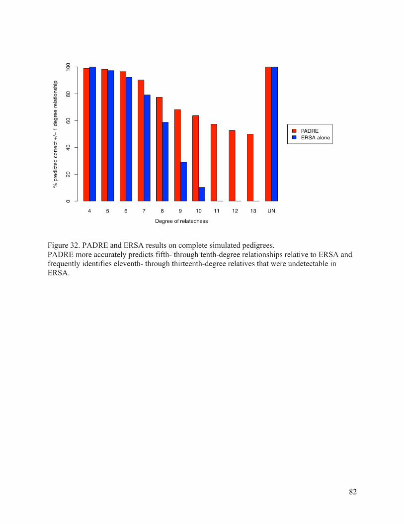
82
Figure 32. PADRE and ERSA results on complete simulated pedigrees. PADRE more accurately predicts fifth- through tenth-degree relationships relative to ERSA and frequently identifies eleventh- through thirteenth-degree relatives that were undetectable in ERSA.

83
Figure 33. Percentage of correct relationship estimations by PADRE on extended European ancestry pedigrees compared to the simulated pedigree results. The accuracy observed in the extended pedigrees as additional first- and second-degree relatives were added was broadly consistent with the simulated pedigree accuracy.
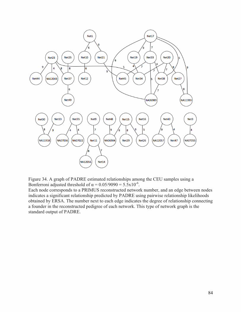
84
Figure 34. A graph of PADRE estimated relationships among the CEU samples using a Bonferroni adjusted threshold of α = 0.05/9090 = 5.5x10⁻⁶. Each node corresponds to a PRIMUS reconstructed network number, and an edge between nodes indicates a significant relationship predicted by PADRE using pairwise relationship likelihoods obtained by ERSA. The number next to each edge indicates the degree of relationship connecting a founder in the reconstructed pedigree of each network. This type of network graph is the standard output of PADRE.
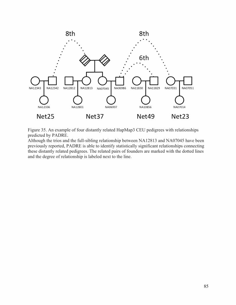
85
Figure 35. An example of four distantly related HapMap3 CEU pedigrees with relationships predicted by PADRE. Although the trios and the full-sibling relationship between NA12813 and NA07045 have been previously reported, PADRE is able to identify statistically significant relationships connecting these distantly related pedigrees. The related pairs of founders are marked with the dotted lines and the degree of relationship is labeled next to the line.

86
Discussion
We have demonstrated through simulations and actual pedigrees that PADRE can leverage
pedigree reconstruction results from PRIMUS and distant pairwise relationship predictions from
ERSA to improve both the power to detect distant relationships and the accuracy of relationship
estimation. The power to detect relationships more distant than ninth-degree relatives is
dependent on the number of generations in the pedigrees that PADRE connects. For instance,
PADRE detected up to thirteenth-degree relationships in the simulated pedigrees because each
pedigree had three generations and the founders of the pedigrees (A2 and B2, Figure 30) were
ninth-degree relatives. It stands to reason that as the depth of the pedigrees being connected by
PADRE increases, so will the distance of relationships that PADRE will be able to predict.
Therefore, we expect that the maximum degree of relationship PADRE can detect is ninth degree
plus the sum of generations in the two pedigrees PADRE connects. PADRE relationship
estimation accuracy improves as the number of genotyped individuals within each pedigree
increases (Figure 31 and Figure 33). PADRE is most accurate when all individuals within a
pedigree are genotyped (Figure 32).
We note that PADRE does not look for distant relationships within the same reconstructed
pedigree structures, as it assumes no consanguinity. However, these types of relationships can be
detected in other ways, for example using ISCA80 and ERSA (v2) to evaluate regions of the
genome that are shared IBD2 between individuals.
Existing pairwise prediction programs use the number and size of shared IBD segments between
two individuals to estimate their degree of relatedness. However, as the degree of relatedness
increases, the number of shared segments drops to zero. Most tenth-degree relatives share no
segments of their autosomal DNA IBD (in humans); therefore, their degree of relatedness cannot
be estimated by existing pairwise comparison programs. PADRE uses reconstructed pedigrees to
estimate relationships between individuals who share no portion of their genomes with detectable
IBD as long as their ancestors can be accurately estimated as ninth-degree relatives or closer.
PADRE provides an immediate benefit to human genetic analysis. This is particularly true in
large case-control studies. Supposedly unrelated individuals can in fact have relationships at the
level of fourth- through thirteenth-degree relatives, and these cryptic relationships can be

87
detected even in small datasets, as shown in our analysis of the CEU data (Figure 34 and Figure
35). By identifying these relationships, studies can avoid artifactual findings due to cryptic
relatedness11. In addition, techniques that explicitly model relationships may provide more
power81, particularly for relatively high penetrance alleles segregating in pedigrees.

88
Chapter 6. Summary and future directions
Significant Contributions
PRIMUS features an implementation of a graph theory algorithm adapted to find the maximum
unrelated set of individuals within a genetic dataset. PRIMUS retains up to 50% more samples
when used over existing and suggested methods.
PRIMUS also features pedigree reconstruction capabilities. It can read in genome-wide estimates
of IBD, and infer the familial relationships from these estimates, and piece these relationships
together to generate all the possible pedigree structures that fit the genetic data. This method
overcomes several of the limitations of other pedigree reconstruction programs and provides a
tool capable of using real world family structures. For instance, of the 10,000 simulated
pedigrees generated to validate PRIMUS, the leading pedigree reconstruction programs could
only reconstruct 43 (<0.5%) while PRIMUS fully reconstructed over 92% of them. PRIMUS can
reconstruct non-consanguineous, multi-generational pedigrees using up to third-degree
relationships, regardless of the pattern of missing samples. PRIMUS even outperformed the
standard programs used for verifying pedigrees by demonstrating that it can more accurately
predict relationships within a pedigree structure when more than 50% of the samples are
genotyped. PRIMUS also allows the user to specify the sex and age of the individuals to improve
the chances of identifying the correct pedigree structure.
PRIMUS is the first pedigree reconstruction program to incorporate genome-wide, high-density
data with mtDNA and non-recombining Y chromosome (NRY) haplotypes. The addition of these
data greatly improves reconstruction by eliminating pedigrees that fit the autosomal inheritance
pattern, but are inconsistent with the inheritance pattern of mtDNA and NRY haplotypes. For
example, one simulated pedigree had 58 pedigree structures that fit the autosomal data, but with
the addition of just mtDNA, PRIMUS was able to identify the true pedigree structure by ruling
out the 57 incompatible structures.
Finally, PRIMUS provides an excellent tool for reconstructing pedigrees using up to third-degree
relationships, but with addition of a new algorithm known as PADRE (Pedigree Aware Distant
Relationship Estimation), I sought a way to connect the reconstructed pedigrees using a distant
89
relationships prediction method: Estimation of Recent Shared Ancestry (ERSA). Importantly,
PADRE extends the relationship predictions beyond the ninth-degree relationship limit of ERSA
alone. With PADRE, predictions to thirteenth-degree were possible within the simulations.
PADRE also improves the accuracy of predictions for fifth- through ninth-degree relationships
by 25% for simulated data compared to ERSA alone.
Future Directions
As sequencing technology continues to improve and drives down the cost of medical sequencing,
I expect that within the next two decades most, if not all, people in developed countries will have
their genomes sequenced. Having access to this level of data would provide unprecedented
power to detect, solve, and treat human genetic diseases. However, this volume of data presents
enormous bioinformatics challenges. The challenge most relevant to my research would be
obtaining and maintaining accurate records of how genetic data match reported family histories
and pedigrees. Pedigree reconstruction with PRIMUS provides an initial solution, but advances
in the field of pedigree reconstruction are necessary in order to handle the volume, distance, and
variety of family relationships found across the entire human population.
PRIMUS was designed to reconstruct pedigrees with first- through third-degree relationships
from outbred populations. However, I believe that pedigree reconstruction can, and must, be
expanded to incorporate three additional classes of relationships: complex, consanguineous, and
distant relationships up to sixth-degree relatives.
Complex relationships
First, complex relationships include double first cousins (i.e., the children of two sisters married
to two brothers) and half-sibling-plus-first-cousin (i.e., children of an individual who had
children with a pair of siblings). Although these relationships are not extremely common in the
United States, they often occur in pedigrees of individuals in other cultures. Both of these
relationships have expected mean IBD proportions that are distinct from the non-complex first-
through third-degree relationships, and they can be incorporated into pedigree reconstruction
using the same framework laid out with PRIMUS.
90
Consanguineous relationships
There are two types of consanguinity that will need to be handled differently. First, there are
recent consanguineous relationships. These relationships will have mean expected IBD
proportions and, therefore, could be accurately predicted using the framework already laid out by
PRIMUS; however, I expect that the IBD estimate distributions for the various consanguineous
relationships will significantly overlap with one another. This problem can be remedied as DNA
from more individuals in the pedigree are collected and genotyped/sequenced. The second type
of consanguinity is an in-bred population background often caused by a bottlenecked and
isolated population, for example the Hutterites82. This consanguineous background results in
individuals looking more closely related to one another than they should be given their recent
family history. One potential solution is to mask regions of the genome common among all
individuals of the population. Another solution may be to identify regions of each individual’s
genome that happen to be detected IBD with many other individuals in the population. The
impact that these regions of the individual’s genome have on IBD estimates can be down
weighted in order to counter act the inbred background affect on IBD estimates. Both of these
potential solutions to the inbred background problem require a substantial amount of sequence or
genotype data for each population of interest in order to know which regions of the genome to
mask or down weight. However, with the continued advancement in sequencing technology and
the amount of data being generated worldwide, this does not seem unrealistic for most
populations within the next decade.
Distant relationships
Distant relationships pose a significant challenge in pedigree reconstruction for two reasons: they
are more challenging to accurately estimate (Figure 31), and there are more relationship types as
the degree of relatedness increases (Supplementary Table 6). However, with improved phasing
and IBD detection, I expect that detection up to sixth-degree relationship can be nearly 100%
accurate since we have power to detect all sixth-degree relationships with the PADRE algorithm
(Figure 2B from PADRE paper). That said, piecing together many sixth-degree relationships
would generate far too many pedigrees. Instead of reconstructing them, fourth- through sixth-
degree relationships could be used to reduce the number of possible pedigrees generated in

91
pedigree reconstruction by eliminating the pedigrees that are inconsistent with the relationship
estimations. Addition of mtDNA and Y haplotypes could also be helpful in piece back together
distant relationships and reducing the number of pedigree structures that fit the genetic data.
Conclusion
The field of human genetics is expanding rapidly and is in need of powerful computational tools
to manage, verify, and leverage the massive datasets being generated. I have developed a
powerful tool called PRIMUS that has proven effective at using several types of genetic data to
reconstruct and verify pedigrees as well as connect distantly related pedigrees with PADRE.
PRIMUS is a big step forward towards tackling the need to reconstruct and verify pedigrees
within large existing datasets like the Jackson Heart Study and the Geisinger Health System.
However, in order to handle the size and wide variety of pedigree structures that exist within the
world’s populations, additional advancements in IBD detection and complex/inbred relationship
reconstruction will be necessary.

92
Web Resources
The URLs for data presented herein are as follows:
Boston Early-Onset COPD Study, http://bostoncopd.org
CraneFoot, http://www.finndiane.fi/software/cranefoot/
GraphViz, www.graphviz.org
International HapMap Project, http://hapmap.ncbi.nlm.nih.gov
IPED2, http://www.cs.ucla.edu/~danhe/Software/IPED2.html
Kinship2, http://cran.r-project.org/package.kinship2
PLINK 1.07, http://pngu.mgh.harvard.edu/purcell/plink/
PRIMUS, http://primus.gs.washington.edu
PRIMUS maximum unrelated set of individuals for the publically available datasets, http://sourceforge.net/projects/primus-beta/datasets/
PRIMUS simulations, the link to the code used for generating simulations, and the reconstructed HapMap3 pedigrees, http://sourceforge.net/projects/primus-beta/files/
SciPy, http://www.scipy.org

93
References
1. Strachan, T., and Read, A. (2010). Human Molecular Genetics, Fourth Edition.(Garland Science).
2. Riordan, J.R., Rommens, J.M., Kerem, B., Alon, N., Rozmahel, R., Grzelczak, Z., Zielenski, J., Lok, S., Plavsic, N., Chou, J.L., et al. (1989). Identification of the cystic fibrosis gene: cloning and characterization of complementary DNA. Science 245, 1066-1073.
3. Hall, J.M., Lee, M.K., Newman, B., Morrow, J.E., Anderson, L.A., Huey, B., and King, M.C. (1990). Linkage of early-onset familial breast cancer to chromosome 17q21. Science 250, 1684-1689.
4. Below, J.E., Earl, D.L., Shively, K.M., McMillin, M.J., Smith, J.D., Turner, E.H., Stephan, M.J., Al-Gazali, L.I., Hertecant, J.L., Chitayat, D., et al. (2013). Whole-genome analysis reveals that mutations in inositol polyphosphate phosphatase-like 1 cause opsismodysplasia. American journal of human genetics 92, 137-143.
5. McMillin, M.J., Below, J.E., Shively, K.M., Beck, A.E., Gildersleeve, H.I., Pinner, J., Gogola, G.R., Hecht, J.T., Grange, D.K., Harris, D.J., et al. (2013). Mutations in ECEL1 cause distal arthrogryposis type 5D. American journal of human genetics 92, 150-156.
6. Makaryan, V., Rosenthal, E.A., Bolyard, A.A., Kelley, M.L., Below, J.E., Bamshad, M.J., Bofferding, K.M., Smith, J.D., Buckingham, K., Boxer, L.A., et al. (2014). TCIRG1-associated congenital neutropenia. Human mutation 35, 824-827.
7. Santorico, S.A., and Edwards, K.L. (2014). Challenges of linkage analysis in the era of whole-genome sequencing. Genet Epidemiol 38 Suppl 1, S92-96.
8. Ott, J., Kamatani, Y., and Lathrop, M. (2011). Family-based designs for genome-wide association studies. Nature reviews Genetics 12, 465-474.
9. Li, B., Krakow, D., Nickerson, D.A., Bamshad, M.J., University of Washington Center for Mendelian, G., Chang, Y., Lachman, R.S., Yilmaz, A., Kayserili, H., and Cohn, D.H. (2014). Opsismodysplasia resulting from an insertion mutation in the SH2 domain, which destabilizes INPPL1. American journal of medical genetics Part A.
10. Welter, D., MacArthur, J., Morales, J., Burdett, T., Hall, P., Junkins, H., Klemm, A., Flicek, P., Manolio, T., Hindorff, L., et al. (2014). The NHGRI GWAS Catalog, a curated resource of SNP-trait associations. Nucleic acids research 42, D1001-1006.
11. Voight, B.F., and Pritchard, J.K. (2005). Confounding from cryptic relatedness in case-control association studies. PLoS genetics 1, e32.
12. Devlin, B., and Roeder, K. (1999). Genomic control for association studies. Biometrics 55, 997-1004.
13. Sun, L., and Dimitromanolakis, A. (2012). Identifying Cryptic Relatedness. In Statistical human genetics : methods and protocols. (New York, Springer), pp 47-57.
14. Patterson, N., Price, A.L., and Reich, D. (2006). Population structure and eigenanalysis. PLoS Genet 2, e190.
15. Thornton, T., and McPeek, M.S. (2010). ROADTRIPS: case-control association testing with partially or completely unknown population and pedigree structure. Am J Hum Genet 86, 172-184.
16. Kang, H.M., Sul, J.H., Service, S.K., Zaitlen, N.A., Kong, S.Y., Freimer, N.B., Sabatti, C., and Eskin, E. (2010). Variance component model to account for sample structure in genome-wide association studies. Nat Genet 42, 348-354.
94
17. Bron, C., and Kerbosch, J. (1973). Algorithm 457: finding all cliques of an undirected graph. Commun ACM 16, 575-577.
18. Staples, J., Nickerson, D.A., and Below, J.E. (2013). Utilizing graph theory to select the largest set of unrelated individuals for genetic analysis. Genet Epidemiol 37, 136-141.
19. Boehnke, M., and Cox, N.J. (1997). Accurate inference of relationships in sib-pair linkage studies. American journal of human genetics 61, 423-429.
20. Bellis, M.A., Hughes, K., Hughes, S., and Ashton, J.R. (2005). Measuring paternal discrepancy and its public health consequences. Journal of epidemiology and community health 59, 749-754.
21. Kerr, S.M., Campbell, A., Murphy, L., Hayward, C., Jackson, C., Wain, L.V., Tobin, M.D., Dominiczak, A., Morris, A., Smith, B.H., et al. (2013). Pedigree and genotyping quality analyses of over 10,000 DNA samples from the Generation Scotland: Scottish Family Health Study. BMC medical genetics 14, 38.
22. Wolf, M., Musch, J., Enczmann, J., and Fischer, J. (2012). Estimating the prevalence of nonpaternity in Germany. Human nature 23, 208-217.
23. Purcell, S., Neale, B., Todd-Brown, K., Thomas, L., Ferreira, M.A., Bender, D., Maller, J., Sklar, P., de Bakker, P.I., Daly, M.J., et al. (2007). PLINK: a tool set for whole-genome association and population-based linkage analyses. American journal of human genetics 81, 559-575.
24. Kyriazopoulou-Panagiotopoulou, S., Kashef Haghighi, D., Aerni, S.J., Sundquist, A., Bercovici, S., and Batzoglou, S. (2011). Reconstruction of genealogical relationships with applications to Phase III of HapMap. Bioinformatics 27, i333-341.
25. Manichaikul, A., Mychaleckyj, J.C., Rich, S.S., Daly, K., Sale, M., and Chen, W.M. (2010). Robust relationship inference in genome-wide association studies. Bioinformatics 26, 2867-2873.
26. Abecasis, G.R., Cherny, S.S., Cookson, W.O.C., and Cardon, L.R. (2001). GRR: graphical representation of relationship errors. Bioinformatics 17, 742-743.
27. Huff, C.D., Witherspoon, D.J., Simonson, T.S., Xing, J.C., Watkins, W.S., Zhang, Y.H., Tuohy, T.M., Neklason, D.W., Burt, R.W., Guthery, S.L., et al. (2011). Maximum-likelihood estimation of recent shared ancestry (ERSA). Genome Res 21, 768-774.
28. Epstein, M.P., Duren, W.L., and Boehnke, M. (2000). Improved inference of relationships for pairs of individuals. American journal of human genetics 67, 1219-1231.
29. Sun, L., Wilder, K., and McPeek, M.S. (2002). Enhanced pedigree error detection. Hum Hered 54, 99-110.
30. Nijmeijer, J.S., Arias-Vasquez, A., Rommelse, N.N., Altink, M.E., Buschgens, C.J., Fliers, E.A., Franke, B., Minderaa, R.B., Sergeant, J.A., Buitelaar, J.K., et al. (2014). Quantitative linkage for autism spectrum disorders symptoms in attention-deficit/hyperactivity disorder: significant locus on chromosome 7q11. Journal of autism and developmental disorders 44, 1671-1680.
31. Chen, C.T., Liu, C.T., Chen, G.K., Andrews, J.S., Arnold, A.M., Dreyfus, J., Franceschini, N., Garcia, M.E., Kerr, K.F., Li, G., et al. (2014). Meta-analysis of loci associated with age at natural menopause in African-American women. Hum Mol Genet 23, 3327-3342.
32. Lange, L.A., Hu, Y., Zhang, H., Xue, C., Schmidt, E.M., Tang, Z.Z., Bizon, C., Lange, E.M., Smith, J.D., Turner, E.H., et al. (2014). Whole-exome sequencing identifies rare and low-frequency coding variants associated with LDL cholesterol. Am J Hum Genet 94, 233-245.

95
33. Bella, J.N., Cole, S.A., Laston, S., Almasy, L., Comuzzie, A., Lee, E.T., Best, L.G., Fabsitz, R.R., Howard, B.V., Maccluer, J.W., et al. (2013). Genome-wide linkage analysis of carotid artery lumen diameter: the strong heart family study. International journal of cardiology 168, 3902-3908.
34. Bizon, C., Spiegel, M., Chasse, S.A., Gizer, I.R., Li, Y., Malc, E.P., Mieczkowski, P.A., Sailsbery, J.K., Wang, X., Ehlers, C.L., et al. (2014). Variant calling in low-coverage whole genome sequencing of a Native American population sample. BMC genomics 15, 85.
35. Quillen, E.E., Chen, X.D., Almasy, L., Yang, F., He, H., Li, X., Wang, X.Y., Liu, T.Q., Hao, W., Deng, H.W., et al. (2014). ALDH2 is associated to alcohol dependence and is the major genetic determinant of "daily maximum drinks" in a GWAS study of an isolated rural chinese sample. American journal of medical genetics Part B, Neuropsychiatric genetics : the official publication of the International Society of Psychiatric Genetics 165B, 103-110.
36. Zhu, Y., Voruganti, V.S., Lin, J., Matsuguchi, T., Blackburn, E., Best, L.G., Lee, E.T., MacCluer, J.W., Cole, S.A., and Zhao, J. (2013). QTL mapping of leukocyte telomere length in American Indians: the Strong Heart Family Study. Aging 5, 704-716.
37. Nolan, D., Kraus, W.E., Hauser, E., Li, Y.J., Thompson, D.K., Johnson, J., Chen, H.C., Nelson, S., Haynes, C., Gregory, S.G., et al. (2013). Genome-wide linkage analysis of cardiovascular disease biomarkers in a large, multigenerational family. PLoS One 8, e71779.
38. Li, H., Glusman, G., Hu, H., Shankaracharya, Caballero, J., Hubley, R., Witherspoon, D., Guthery, S.L., Mauldin, D.E., Jorde, L.B., et al. (2014). Relationship estimation from whole-genome sequence data. PLoS genetics 10, e1004144.
39. Huff, C.D., Witherspoon, D.J., Simonson, T.S., Xing, J., Watkins, W.S., Zhang, Y., Tuohy, T.M., Neklason, D.W., Burt, R.W., Guthery, S.L., et al. (2011). Maximum-likelihood estimation of recent shared ancestry (ERSA). Genome research 21, 768-774.
40. Browning, S.R., and Browning, B.L. (2010). High-resolution detection of identity by descent in unrelated individuals. Am J Hum Genet 86, 526-539.
41. Han, L., and Abney, M. (2011). Identity by descent estimation with dense genome-wide genotype data. Genet Epidemiol 35, 557-567.
42. Browning, B.L., and Browning, S.R. (2011). A fast, powerful method for detecting identity by descent. American journal of human genetics 88, 173-182.
43. Kong, A., Masson, G., Frigge, M.L., Gylfason, A., Zusmanovich, P., Thorleifsson, G., Olason, P.I., Ingason, A., Steinberg, S., Rafnar, T., et al. (2008). Detection of sharing by descent, long-range phasing and haplotype imputation. Nat Genet 40, 1068-1075.
44. Pemberton, T.J., Wang, C., Li, J.Z., and Rosenberg, N.A. (2010). Inference of unexpected genetic relatedness among individuals in HapMap Phase III. American journal of human genetics 87, 457-464.
45. Manichaikul, A., Palmas, W., Rodriguez, C.J., Peralta, C.A., Divers, J., Guo, X., Chen, W.M., Wong, Q., Williams, K., Kerr, K.F., et al. (2012). Population structure of hispanics in the United States: the multi-ethnic study of atherosclerosis. PLoS Genet 8, e1002640.
46. Brandstadt, A. (1998). Partitions of graphs into one or two independent sets and cliques (vol 152, pg 47, 1996). Discrete Math 186, 295-295.
47. Calzals, F., and Karande, C. (2008). A note on the problem of reporting maximal cliques. Theor Comput Sci 407, 564-568.
96
48. Cazals, F., and Karande, C. (2008). A note on the problem of reporting maximal cliques. Theoretical Computer Science 407, 564-568.
49. Stanford, J.L., FitzGerald, L.M., McDonnell, S.K., Carlson, E.E., McIntosh, L.M., Deutsch, K., Hood, L., Ostrander, E.A., and Schaid, D.J. (2009). Dense genome-wide SNP linkage scan in 301 hereditary prostate cancer families identifies multiple regions with suggestive evidence for linkage. Hum Mol Genet 18, 1839-1848.
50. Consotium, T.I.H., Altshuler, D.M., Gibbs, R.A., Peltonen, L., Dermitzakis, E., Schaffner, S.F., Yu, F., Bonnen, P.E., de Bakker, P.I., Deloukas, P., et al. (2010). Integrating common and rare genetic variation in diverse human populations. Nature 467, 52-58.
51. Consortium, T.G.P. (2010). A map of human genome variation from population-scale sequencing. Nature 467, 1061-1073.
52. Heath, S.C., Gut, I.G., Brennan, P., McKay, J.D., Bencko, V., Fabianova, E., Foretova, L., Georges, M., Janout, V., Kabesch, M., et al. (2008). Investigation of the fine structure of European populations with applications to disease association studies. Eur J Hum Genet 16, 1413-1429.
53. Day-Williams, A.G., Blangero, J., Dyer, T.D., Lange, K., and Sobel, E.M. (2011). Linkage analysis without defined pedigrees. Genet Epidemiol 35, 360-370.
54. Riester, M., Stadler, P.F., and Klemm, K. (2009). FRANz: reconstruction of wild multi-generation pedigrees. Bioinformatics 25, 2134-2139.
55. Hadfield, J.D., Richardson, D.S., and Burke, T. (2006). Towards unbiased parentage assignment: combining genetic, behavioural and spatial data in a Bayesian framework. Mol Ecol 15, 3715-3730.
56. Marshall, T.C., Slate, J., Kruuk, L.E.B., and Pemberton, J.M. (1998). Statistical confidence for likelihood-based paternity inference in natural populations. Mol Ecol 7, 639-655.
57. Cussens, J., Bartlett, M., Jones, E.M., and Sheehan, N.A. (2013). Maximum Likelihood Pedigree Reconstruction Using Integer Linear Programming. Genet Epidemiol 37, 69-83.
58. He, D., Wang, Z., Han, B., Parida, L., and Eskin, E. (2013). IPED: inheritance path-based pedigree reconstruction algorithm using genotype data. J Comput Biol 20, 780-791.
59. Kirkpatrick, B., Li, S.C., Karp, R.M., and Halperin, E. (2011). Pedigree reconstruction using identity by descent. Journal of computational biology : a journal of computational molecular cell biology 18, 1481-1493.
60. Shem-Tov, D., and Halperin, E. (2014). Historical pedigree reconstruction from extant populations using PArtitioning of RElatives (PREPARE). PLoS computational biology 10, e1003610.
61. Morrison, J. (2013). Characterization and correction of error in genome-wide IBD estimation for samples with population structure. Genet Epidemiol 37, 635-641.
62. Thornton, T., Tang, H., Hoffmann, T.J., Ochs-Balcom, H.M., Caan, B.J., and Risch, N. (2012). Estimating kinship in admixed populations. American journal of human genetics 91, 122-138.
63. Abecasis, G.R., Cherny, S.S., Cookson, W.O., and Cardon, L.R. (2002). Merlin--rapid analysis of dense genetic maps using sparse gene flow trees. Nature genetics 30, 97-101.
64. Hill, W.G., and Weir, B.S. (2011). Variation in actual relationship as a consequence of Mendelian sampling and linkage. Genetics research 93, 47-64.
65. Makinen, V.P., Parkkonen, M., Wessman, M., Groop, P.H., Kanninen, T., and Kaski, K. (2005). High-throughput pedigree drawing. Eur J Hum Genet 13, 987-989.
97
66. Below, J.E., Gamazon, E.R., Morrison, J.V., Konkashbaev, A., Pluzhnikov, A., McKeigue, P.M., Parra, E.J., Elbein, S.C., Hallman, D.M., Nicolae, D.L., et al. (2011). Genome-wide association and meta-analysis in populations from Starr County, Texas, and Mexico City identify type 2 diabetes susceptibility loci and enrichment for expression quantitative trait loci in top signals. Diabetologia 54, 2047-2055.
67. Silverman, E.K., Chapman, H.A., Drazen, J.M., Weiss, S.T., Rosner, B., Campbell, E.J., O'Donnell, W.J., Reilly, J.J., Ginns, L., Mentzer, S., et al. (1998). Genetic epidemiology of severe, early-onset chronic obstructive pulmonary disease. Risk to relatives for airflow obstruction and chronic bronchitis. American journal of respiratory and critical care medicine 157, 1770-1778.
68. Fu, W., O'Connor, T.D., Jun, G., Kang, H.M., Abecasis, G., Leal, S.M., Gabriel, S., Rieder, M.J., Altshuler, D., Shendure, J., et al. (2013). Analysis of 6,515 exomes reveals the recent origin of most human protein-coding variants. Nature 493, 216-220.
69. Li, H., and Durbin, R. (2009). Fast and accurate short read alignment with Burrows-Wheeler transform. Bioinformatics 25, 1754-1760.
70. McKenna, A., Hanna, M., Banks, E., Sivachenko, A., Cibulskis, K., Kernytsky, A., Garimella, K., Altshuler, D., Gabriel, S., Daly, M., et al. (2010). The Genome Analysis Toolkit: a MapReduce framework for analyzing next-generation DNA sequencing data. Genome Res 20, 1297-1303.
71. Danecek, P., Auton, A., Abecasis, G., Albers, C.A., Banks, E., DePristo, M.A., Handsaker, R.E., Lunter, G., Marth, G.T., Sherry, S.T., et al. (2011). The variant call format and VCFtools. Bioinformatics 27, 2156-2158.
72. Consotium, T.I.H. (2010). Integrating common and rare genetic variation in diverse human populations. Nature 467, 52-58.
73. Cross, D.S., Ivacic, L.C., Stefanski, E.L., and McCarty, C.A. (2010). Population based allele frequencies of disease associated polymorphisms in the Personalized Medicine Research Project. BMC genetics 11, 51.
74. Staples, J., Qiao, D., Cho, M.H., Silverman, E.K., Genomics, U.o.W.C.f.M., Nickerson, D.A., and Below, J.E. (2014). PRIMUS: Rapid reconstruction of pedigrees from genome-wide estimates of identity by descent. American journal of human genetics 95, 553-564.
75. Lippold, S., Xu, H., Ko, A., Li, M., Renaud, G., Butthof, A., Schroder, R., and Stoneking, M. (2014). Human paternal and maternal demographic histories: insights from high-resolution Y chromosome and mtDNA sequences. Investigative genetics 5, 13.
76. Alvarez-Cubero, M.J., Saiz, M., Martinez-Gonzalez, L.J., Alvarez, J.C., Eisenberg, A.J., Budowle, B., and Lorente, J.A. (2012). Genetic identification of missing persons: DNA analysis of human remains and compromised samples. Pathobiology : journal of immunopathology, molecular and cellular biology 79, 228-238.
77. Lin, T.H., Myers, E.W., and Xing, E.P. (2006). Interpreting anonymous DNA samples from mass disasters--probabilistic forensic inference using genetic markers. Bioinformatics 22, e298-306.
78. Browning, S.R., and Browning, B.L. (2007). Rapid and accurate haplotype phasing and missing-data inference for whole-genome association studies by use of localized haplotype clustering. Am J Hum Genet 81, 1084-1097.
79. Gusev, A., Lowe, J.K., Stoffel, M., Daly, M.J., Altshuler, D., Breslow, J.L., Friedman, J.M., and Pe'er, I. (2009). Whole population, genome-wide mapping of hidden relatedness. Genome research 19, 318-326.
98
80. Roach, J.C., Glusman, G., Smit, A.F., Huff, C.D., Hubley, R., Shannon, P.T., Rowen, L., Pant, K.P., Goodman, N., Bamshad, M., et al. (2010). Analysis of genetic inheritance in a family quartet by whole-genome sequencing. Science 328, 636-639.
81. Hu, H., Roach, J.C., Coon, H., Guthery, S.L., Voelkerding, K.V., Margraf, R.L., Durtschi, J.D., Tavtigian, S.V., Shankaracharya, Wu, W., et al. (2014). A unified test of linkage analysis and rare-variant association for analysis of pedigree sequence data. Nature biotechnology 32, 663-669.
82. Campbell, C.D., Chong, J.X., Malig, M., Ko, A., Dumont, B.L., Han, L., Vives, L., O'Roak, B.J., Sudmant, P.H., Shendure, J., et al. (2012). Estimating the human mutation rate using autozygosity in a founder population. Nature genetics 44, 1277-1281.
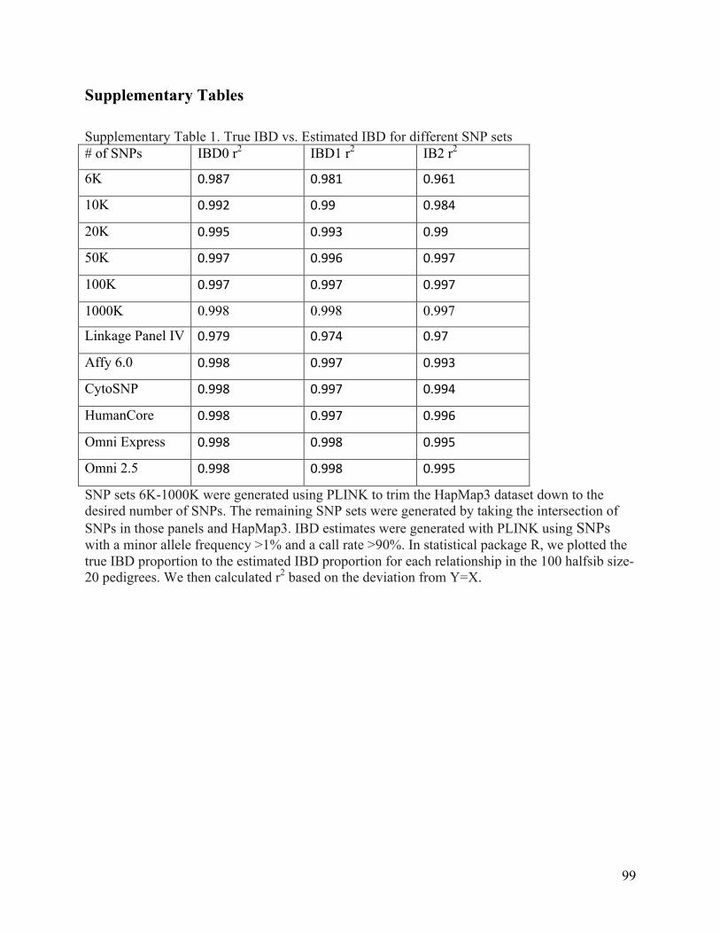
99
Supplementary Tables
Supplementary Table 1. True IBD vs. Estimated IBD for different SNP sets # of SNPs IBD0 r2 IBD1 r2 IB2 r2
6K 0.987 0.981 0.961
10K 0.992 0.99 0.984
20K 0.995 0.993 0.99
50K 0.997 0.996 0.997
100K 0.997 0.997 0.997
1000K 0.998 0.998 0.997
Linkage Panel IV 0.979 0.974 0.97
Affy 6.0 0.998 0.997 0.993
CytoSNP 0.998 0.997 0.994
HumanCore 0.998 0.997 0.996
Omni Express 0.998 0.998 0.995
Omni 2.5 0.998 0.998 0.995
SNP sets 6K-1000K were generated using PLINK to trim the HapMap3 dataset down to the desired number of SNPs. The remaining SNP sets were generated by taking the intersection of SNPs in those panels and HapMap3. IBD estimates were generated with PLINK using SNPs with a minor allele frequency >1% and a call rate >90%. In statistical package R, we plotted the true IBD proportion to the estimated IBD proportion for each relationship in the 100 halfsib size-20 pedigrees. We then calculated r2 based on the deviation from Y=X.
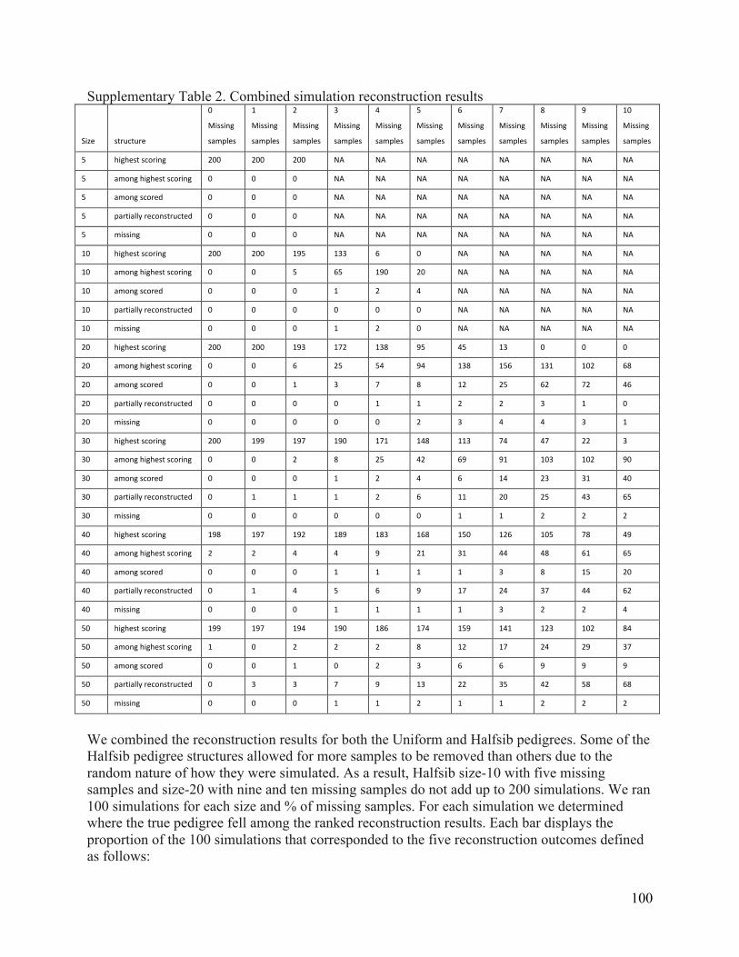
100
Supplementary Table 2. Combined simulation reconstruction results
Size structure
0
Missing
samples
1
Missing
samples
2
Missing
samples
3
Missing
samples
4
Missing
samples
5
Missing
samples
6
Missing
samples
7
Missing
samples
8
Missing
samples
9
Missing
samples
10
Missing
samples
5 highest scoring 200 200 200 NA NA NA NA NA NA NA NA
5 among highest scoring 0 0 0 NA NA NA NA NA NA NA NA
5 among scored 0 0 0 NA NA NA NA NA NA NA NA
5 partially reconstructed 0 0 0 NA NA NA NA NA NA NA NA
5 missing 0 0 0 NA NA NA NA NA NA NA NA
10 highest scoring 200 200 195 133 6 0 NA NA NA NA NA
10 among highest scoring 0 0 5 65 190 20 NA NA NA NA NA
10 among scored 0 0 0 1 2 4 NA NA NA NA NA
10 partially reconstructed 0 0 0 0 0 0 NA NA NA NA NA
10 missing 0 0 0 1 2 0 NA NA NA NA NA
20 highest scoring 200 200 193 172 138 95 45 13 0 0 0
20 among highest scoring 0 0 6 25 54 94 138 156 131 102 68
20 among scored 0 0 1 3 7 8 12 25 62 72 46
20 partially reconstructed 0 0 0 0 1 1 2 2 3 1 0
20 missing 0 0 0 0 0 2 3 4 4 3 1
30 highest scoring 200 199 197 190 171 148 113 74 47 22 3
30 among highest scoring 0 0 2 8 25 42 69 91 103 102 90
30 among scored 0 0 0 1 2 4 6 14 23 31 40
30 partially reconstructed 0 1 1 1 2 6 11 20 25 43 65
30 missing 0 0 0 0 0 0 1 1 2 2 2
40 highest scoring 198 197 192 189 183 168 150 126 105 78 49
40 among highest scoring 2 2 4 4 9 21 31 44 48 61 65
40 among scored 0 0 0 1 1 1 1 3 8 15 20
40 partially reconstructed 0 1 4 5 6 9 17 24 37 44 62
40 missing 0 0 0 1 1 1 1 3 2 2 4
50 highest scoring 199 197 194 190 186 174 159 141 123 102 84
50 among highest scoring 1 0 2 2 2 8 12 17 24 29 37
50 among scored 0 0 1 0 2 3 6 6 9 9 9
50 partially reconstructed 0 3 3 7 9 13 22 35 42 58 68
50 missing 0 0 0 1 1 2 1 1 2 2 2
We combined the reconstruction results for both the Uniform and Halfsib pedigrees. Some of the Halfsib pedigree structures allowed for more samples to be removed than others due to the random nature of how they were simulated. As a result, Halfsib size-10 with five missing samples and size-20 with nine and ten missing samples do not add up to 200 simulations. We ran 100 simulations for each size and % of missing samples. For each simulation we determined where the true pedigree fell among the ranked reconstruction results. Each bar displays the proportion of the 100 simulations that corresponded to the five reconstruction outcomes defined as follows:

101
“highest scoring” – The true pedigree is the highest scoring pedigree “among highest scoring” – PRIMUS output contained more than one possible pedigree and the true pedigree is tied as the highest scoring pedigree with one or more other pedigrees “among scored” – the true pedigree is not the highest scoring pedigree, but is among the pedigrees generated by PRIMUS “partial reconstruction” – the complete reconstruction either resulted in too many possible pedigrees, ran out of memory, or took longer than 36 hours to run and as a result only a partial reconstruction using 1st degree relationships was generated “missing” – PRIMUS reconstructed one or more possible pedigrees, but the true pedigree was not among them
Supplementary Table 3. The accuracy of PRIMUS and RELPAIR relationship predictions with Halfsib size-20 pedigrees
PRIMUS
Percent Missing
samples 0% 5% 10% 15% 20% 25% 30% 35% 40%
1st degree category 100.00% 100.00% 100.00% 100.00% 100.00% 100.00% 100.00% 100.00% 100.00%
2nd degree category 100.00% 100.00% 100.00% 100.00% 99.79% 99.63% 99.55% 99.35% 99.55%
3rd degree category 100.00% 100.00% 100.00% 99.79% 98.81% 99.26% 98.30% 96.27% 93.37%
Distantly/unrelated 100.00% 100.00% 100.00% 100.00% 100.00% 100.00% 100.00% 100.00% 100.00%
1st degree
relationship type 100.00% 100.00% 100.00% 100.00% 100.00% 100.00% 100.00% 100.00% 100.00%
2nd degree
relationship type 100.00% 100.00% 99.37% 97.12% 96.00% 88.45% 75.61% 66.88% 58.48%
3rd degree
relationship type 100.00% 100.00% 98.13% 95.42% 92.46% 85.68% 63.67% 46.73% 26.54%
1st degree
relationship type +
direction 100.00% 100.00% 100.00% 99.86% 99.84% 99.57% 99.54% 99.52% 99.92%
2nd degree
relationship type +
direction 100.00% 100.00% 99.41% 97.80% 96.89% 91.18% 80.92% 73.76% 61.95%
3rd degree
relationship type +
direction 100.00% 100.00% 96.87% 93.37% 91.90% 86.43% 68.29% 45.41% 14.15%
RELPAIR
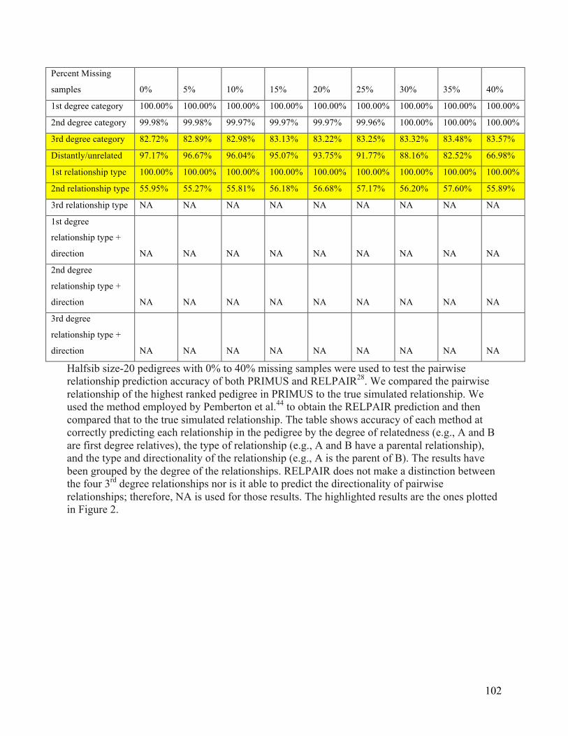
102
Percent Missing
samples 0% 5% 10% 15% 20% 25% 30% 35% 40%
1st degree category 100.00% 100.00% 100.00% 100.00% 100.00% 100.00% 100.00% 100.00% 100.00%
2nd degree category 99.98% 99.98% 99.97% 99.97% 99.97% 99.96% 100.00% 100.00% 100.00%
3rd degree category 82.72% 82.89% 82.98% 83.13% 83.22% 83.25% 83.32% 83.48% 83.57%
Distantly/unrelated 97.17% 96.67% 96.04% 95.07% 93.75% 91.77% 88.16% 82.52% 66.98%
1st relationship type 100.00% 100.00% 100.00% 100.00% 100.00% 100.00% 100.00% 100.00% 100.00%
2nd relationship type 55.95% 55.27% 55.81% 56.18% 56.68% 57.17% 56.20% 57.60% 55.89%
3rd relationship type NA NA NA NA NA NA NA NA NA
1st degree
relationship type +
direction NA NA NA NA NA NA NA NA NA
2nd degree
relationship type +
direction NA NA NA NA NA NA NA NA NA
3rd degree
relationship type +
direction NA NA NA NA NA NA NA NA NA
Halfsib size-20 pedigrees with 0% to 40% missing samples were used to test the pairwise relationship prediction accuracy of both PRIMUS and RELPAIR28. We compared the pairwise relationship of the highest ranked pedigree in PRIMUS to the true simulated relationship. We used the method employed by Pemberton et al.44 to obtain the RELPAIR prediction and then compared that to the true simulated relationship. The table shows accuracy of each method at correctly predicting each relationship in the pedigree by the degree of relatedness (e.g., A and B are first degree relatives), the type of relationship (e.g., A and B have a parental relationship), and the type and directionality of the relationship (e.g., A is the parent of B). The results have been grouped by the degree of the relationships. RELPAIR does not make a distinction between the four 3rd degree relationships nor is it able to predict the directionality of pairwise relationships; therefore, NA is used for those results. The highlighted results are the ones plotted in Figure 2.

103
Supplementary Table 4. EOCOPD pedigree reconstruction summary
Fam FID
Reconstructe
d Correctly
Number of
Genotyped
Samples
Reconstructed
FIDs
Expected
Pedigree
Rank
Number
of
Possible
Pedigrees Explanation
Fam1 1 11 1 1 2
Fam2 1 8 2 1 1
Fam3 1 13 3 2 2
Fam4 1 3 4 1 1
Fam5 1 15 5 1 1
Fam6 0 9 6 NA 20
NON PATERNITY
CAUGHT: half sib
is actually full sib
Fam7 1 10 7 20 28
Fam8 1 9 8 1 1
Fam9 1 8 9 1 1
Fam10 1 9 10 1 1
Fam11 1 4 11 3 7
Fam12 1 2 12 1 1
Fam13 1 3 13 1 1
Fam14 1 5 14 1 1
Fam15 1 2 15 2 2
Fam16 1 2 16 1 1
Fam17 1 8 17 1 1
Fam18 1 6 18 1 2
Fam19 1 5 19 32 33
Fam20 1 15 20 4 11
Fam21 1 5 21 1 1
Fam22 1 13 22 1 2
Fam23 1 8 23 2 3
Fam24 0 10 24 NA 5 NON PATERNITY

104
CAUGHT: half
avuncular instead of
avuncular
Fam25 1 5 25 1 1
Fam26 1 6 26 1 2
Fam27 1 6 27 1 1
Fam28 1 14 28 1 1
Fam29 1 3 29 1 1
Fam30 1 11 30 1 2
Fam31 1 5 31 1 1
Fam32 0 6 32 NA 4
NON PATERNITY
CAUGHT
Fam33 1 3 33 1 1
Fam34 1 4 34 1 4
Fam35 0 6 35,39 NA 1
Sample missing
because of
duplicate; Also non-
paternity;
Fam36 1 3 36 1 1
Fam37 1 2 37 2 5
Fam38 1 3 38 1 1
Fam39 1 15 39 3 3
Contains duplicate
sample
Fam40 1 5 40 1 1
Fam41 1 6 41 1 3
Fam42 1 5 42 1 1
Fam43 1 9 43 4 6
Fam44 1 14 44 1 2
Fam45 0 7 45 NA 1
NON PATERNITY
CAUGHT

105
Fam46 1 3 46 1 1
Fam47 1 6 47 4 4
Fam48 1 4 48 1 1
Fam49 1 10 49 1 1

106
Supplementary Table 5. Comparison of HapMap3 pairwise relationships Population Network IID1 Sex
Hapmap
Reported
PRIMUS
Predicted
Pemberton
Predicted
CARROT
Predicted IID2 Sex
Hapmap
Reported
PRIMUS
Predicted
Pemberton
Predicted
CARROT
Predicted Notes
ASW 1 NA19916 M P P O,P -‐ NA19918 M O O O,P -‐
ASW 1 NA19917 F P P O,P -‐ NA19918 M O O O,P -‐
ASW 2 NA19834 M P P O,P -‐ NA19836 F O O O,P -‐
ASW 2 NA19835 F P P O,P -‐ NA19836 F O O O,P -‐
ASW 3 NA20279 M -‐ O O,P -‐ NA20282 F -‐ P O,P -‐
ASW 3 NA20279 M -‐ H H -‐ NA20284 M -‐ H H -‐ R*
ASW 3 NA20279 M -‐ N N -‐ NA20301 F -‐ A A -‐ R
ASW 3 NA20279 M -‐ 1C -‐ 1C NA20302 M -‐ 1C -‐ 1C
ASW 3 NA20282 F P P O,P -‐ NA20284 M O O O,P -‐
ASW 3 NA20282 F -‐ F F -‐ NA20301 F -‐ F F -‐
ASW 3 NA20282 F -‐ A A -‐ NA20302 M -‐ N N -‐ R*
ASW 3 NA20284 M -‐ N N -‐ NA20301 F -‐ A A -‐ R
ASW 3 NA20284 M -‐ 1C -‐ 1C NA20302 M -‐ 1C -‐ 1C
ASW 3 NA20301 F P P O,P -‐ NA20302 M O O O,P -‐
ASW 4 NA19703 M P P O,P -‐ NA19705 M O O O,P -‐
ASW 4 NA19704 F P P O,P -‐ NA19705 M O O O,P -‐
ASW 6 NA19900 M P P O,P -‐ NA19902 F O O O,P -‐
ASW 6 NA19901 F P P O,P -‐ NA19902 F O O O,P -‐
ASW 9 NA20287 F P O,P O,P -‐ NA20288 M O O,P O,P -‐
ASW 14 NA19713 F -‐ A A -‐ NA19714 F -‐ N N -‐ R
ASW 14 NA19713 F P P O,P -‐ NA19983 F O O O,P -‐
ASW 14 NA19713 F -‐ F F -‐ NA19985 F -‐ F F -‐ R
ASW 14 NA19714 F -‐ 1C -‐ 1C NA19983 F -‐ 1C -‐ 1C
ASW 14 NA19714 F O O O,P -‐ NA19985 F P P O,P -‐
ASW 14 NA19982 M P P O,P -‐ NA19983 F O O O,P -‐
ASW 14 NA19983 F -‐ N N -‐ NA19985 F -‐ A A -‐ R*
ASW 15 NA20340 M -‐
1C,GA,GC
,GG,GN,H
A,HN,UN -‐ U NA20344 F -‐
1C,GA,GC
,GG,GN,H
A,HN,UN -‐ U
ASW 15 NA20340 M -‐
1C,GA,GC
,GG,GN,H
A,HN,UN -‐ -‐ NA20349 M -‐
1C,GA,GC
,GG,GN,H
A,HN,UN -‐ -‐ N
ASW 15 NA20344 F P P O,P -‐ NA20345 M O O O,P -‐
ASW 15 NA20344 F -‐ F F -‐ NA20349 M -‐ F F -‐
ASW 15 NA20344 F -‐ A A -‐ NA20350 M -‐ N N -‐ R
ASW 15 NA20345 M -‐ N N -‐ NA20349 M -‐ A A -‐ R*
ASW 15 NA20345 M -‐ 1C -‐ 1C NA20350 M -‐ 1C -‐ 1C
ASW 15 NA20349 M P P O,P -‐ NA20350 M O O O,P -‐
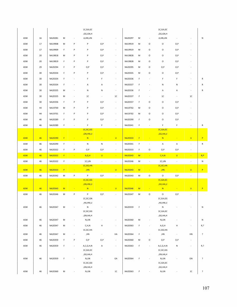
107
ASW 16 NA20281 M -‐
1C,GA,GC
,GG,GN,H
A,HN,UN -‐ -‐ NA20297 M -‐
1C,GA,GC
,GG,GN,H
A,HN,UN -‐ -‐ N
ASW 17 NA19908 M P P O,P -‐ NA19919 M O O O,P -‐
ASW 17 NA19909 F P P O,P -‐ NA19919 M O O O,P -‐
ASW 20 NA19818 M P P O,P -‐ NA19828 M O O O,P -‐
ASW 20 NA19819 F P P O,P -‐ NA19828 M O O O,P -‐
ASW 29 NA20294 F P O,P O,P -‐ NA20295 M O O,P O,P -‐
ASW 30 NA20334 F P P O,P -‐ NA20335 M O O O,P -‐
ASW 30 NA20334 F -‐ F F -‐ NA20336 F -‐ F F -‐ R
ASW 30 NA20334 F -‐ A A -‐ NA20337 F -‐ N N -‐ R
ASW 30 NA20335 M -‐ N N -‐ NA20336 F -‐ A A -‐ R
ASW 30 NA20335 M -‐ 1C -‐ 1C NA20337 F -‐ 1C -‐ 1C
ASW 30 NA20336 F P P O,P -‐ NA20337 F O O O,P -‐
ASW 44 NA19700 M P P O,P -‐ NA19702 M O O O,P -‐
ASW 44 NA19701 F P P O,P -‐ NA19702 M O O O,P -‐
ASW 46 NA20289 F P P O,P -‐ NA20290 F O O O,P -‐
ASW 46 NA20289 F -‐ F F -‐ NA20341 F -‐ F F -‐ R
ASW 46 NA20290 F -‐
1C,GC,GG
,GN,HN,U
N -‐ U NA20333 F -‐
1C,GA,GC
,GG,HA,U
N -‐ U P
ASW 46 NA20290 F -‐ N N -‐ NA20341 F -‐ A A -‐ R
ASW 46 NA20332 F P O,P O,P -‐ NA20333 F O O,P O,P -‐
ASW 46 NA20332 F -‐ A,G,H U -‐ NA20343 M -‐ C,H,N U -‐ R,P
ASW 46 NA20332 F -‐ 1C,UN -‐ -‐ NA20346 M -‐ 1C,UN -‐ -‐ N
ASW 46 NA20333 F -‐
1C,GG,HA
,HN -‐ U NA20343 M -‐
1C,GC,HA
,HN -‐ U P
ASW 46 NA20342 M P P O,P -‐ NA20343 M O O O,P -‐
ASW 46 NA20343 M -‐
1C,GC,GG
,GN,HN,U
N -‐ U NA20346 M -‐
1C,GA,GC
,GG,HA,U
N -‐ U P
ASW 46 NA20346 M P P O,P -‐ NA20347 M O O O,P -‐
ASW 46 NA20347 M -‐
1C,GC,GN
,HA,HN,U
N -‐ -‐ NA20359 F -‐
1C,GA,GG
,HA,HN,U
N -‐ -‐ N
ASW 46 NA20347 M -‐
1C,GC,GG
,GN,HA,H
N,UN -‐ -‐ NA20360 M -‐
1C,GA,GC
,GG,HA,H
N,UN -‐ -‐ N
ASW 46 NA20347 M -‐ C,H,N H -‐ NA20363 F -‐ A,G,H H -‐ R,?
ASW 46 NA20347 M -‐
1C,GC,HA
,HN -‐ HA NA20364 F -‐
1C,GG,HA
,HN -‐ HN ?
ASW 46 NA20359 F P O,P O,P -‐ NA20360 M O O,P O,P -‐
ASW 46 NA20359 F -‐ A,C,G,H,N A -‐ NA20363 F -‐ A,C,G,H,N N -‐ R,?
ASW 46 NA20359 F -‐
1C,GA,GC
,GG,HA,H
N,UN -‐ GA NA20364 F -‐
1C,GC,GG
,GN,HA,H
N,UN -‐ GN ?
ASW 46 NA20360 M -‐
1C,GC,GG
,GN,HA,H
N,UN -‐ 1C NA20363 F -‐
1C,GA,GC
,GG,HA,H
N,UN -‐ 1C ?

108
ASW 46 NA20363 F P O,P O,P -‐ NA20364 F O O,P O,P -‐
ASW 48 NA20356 M P P O,P -‐ NA20358 M O O O,P -‐
ASW 48 NA20357 F P P O,P -‐ NA20358 M O O O,P -‐
ASW 49 NA20291 M P O,P O,P -‐ NA20292 F O O,P O,P -‐
ASW 62 NA19921 F P O,P O,P -‐ NA20129 F O O,P O,P -‐
ASW 65 NA20317 F P O,P O,P -‐ NA20319 F O O,P O,P -‐
ASW 71 NA20126 M P P O,P -‐ NA20128 F O O O,P -‐
ASW 71 NA20127 F P P O,P -‐ NA20128 F O O O,P -‐
ASW 74 NA19914 F P O,P O,P -‐ NA19915 M O O,P O,P -‐
ASW 80 NA20276 F P O,P O,P -‐ NA20277 F O O,P O,P -‐
CEU 1 NA10865 M O O O,P -‐ NA11891 M P P O,P -‐
CEU 1 NA10865 M O O O,P -‐ NA11892 F P P O,P -‐
CEU 8 NA10836 F O O,P O,P -‐ NA12275 F P O,P O,P -‐
CEU 12 NA10852 F O O,P O,P -‐ NA12045 M P O,P O,P -‐
CEU 22 NA10837 M O O O,P -‐ NA12272 M P P O,P -‐
CEU 22 NA10837 M O O O,P -‐ NA12273 F P P O,P -‐
CEU 26 NA12766 M O O O,P -‐ NA12775 M P P O,P -‐
CEU 26 NA12766 M O O O,P -‐ NA12776 F P P O,P -‐
CEU 27 NA12344 M O O O,P -‐ NA12347 M P P O,P -‐
CEU 27 NA12344 M O O O,P -‐ NA12348 F P P O,P -‐
CEU 28 NA12817 M O O O,P -‐ NA12827 M P P O,P -‐
CEU 28 NA12817 M O O O,P -‐ NA12828 F P P O,P -‐
CEU 29 NA10840 F O O O,P -‐ NA12286 M P P O,P -‐
CEU 29 NA10840 F O O O,P -‐ NA12287 F P P O,P -‐
CEU 32 NA12708 F O O,P O,P -‐ NA12718 F P O,P O,P -‐
CEU 37 NA06995 M O O O,P -‐ NA07037 F P P O,P -‐
CEU 37 NA06995 M O O O,P -‐ NA07435 M P P O,P -‐
CEU 44 NA12375 M O O,P O,P -‐ NA12383 F P O,P O,P -‐
CEU 46 NA12335 M O O O,P -‐ NA12340 M P P O,P -‐
CEU 46 NA12335 M O O O,P -‐ NA12341 F P P O,P -‐
CEU 47 NA12767 F O O O,P -‐ NA12777 M P P O,P -‐
CEU 47 NA12767 F O O O,P -‐ NA12778 F P P O,P -‐
CEU 50 NA12877 M O O O,P -‐ NA12889 M P P O,P -‐
CEU 50 NA12877 M O O O,P -‐ NA12890 F P P O,P -‐
CEU 52 NA07346 F P P O,P -‐ NA07349 M O O O,P -‐
CEU 52 NA07347 M P P O,P -‐ NA07349 M O O O,P -‐
CEU 54 NA12739 M O O O,P -‐ NA12748 M P P O,P -‐
CEU 54 NA12739 M O O O,P -‐ NA12749 F P P O,P -‐
CEU 55 NA10864 F O O O,P -‐ NA11893 M P P O,P -‐
CEU 55 NA10864 F O O O,P -‐ NA11894 F P P O,P -‐
CEU 59 NA10853 M O O,P O,P -‐ NA11843 M P O,P O,P -‐
CEU 61 NA12818 F O O O,P -‐ NA12829 M P P O,P -‐
CEU 61 NA12818 F O O O,P -‐ NA12830 F P P O,P -‐
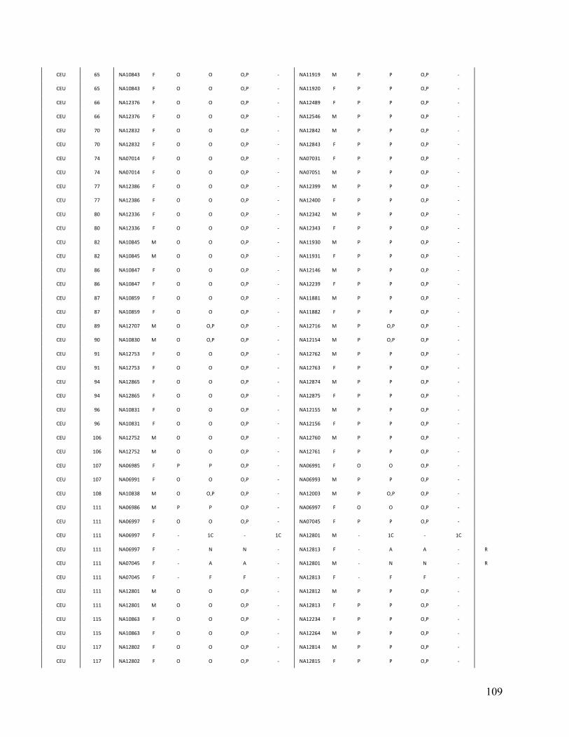
109
CEU 65 NA10843 F O O O,P -‐ NA11919 M P P O,P -‐
CEU 65 NA10843 F O O O,P -‐ NA11920 F P P O,P -‐
CEU 66 NA12376 F O O O,P -‐ NA12489 F P P O,P -‐
CEU 66 NA12376 F O O O,P -‐ NA12546 M P P O,P -‐
CEU 70 NA12832 F O O O,P -‐ NA12842 M P P O,P -‐
CEU 70 NA12832 F O O O,P -‐ NA12843 F P P O,P -‐
CEU 74 NA07014 F O O O,P -‐ NA07031 F P P O,P -‐
CEU 74 NA07014 F O O O,P -‐ NA07051 M P P O,P -‐
CEU 77 NA12386 F O O O,P -‐ NA12399 M P P O,P -‐
CEU 77 NA12386 F O O O,P -‐ NA12400 F P P O,P -‐
CEU 80 NA12336 F O O O,P -‐ NA12342 M P P O,P -‐
CEU 80 NA12336 F O O O,P -‐ NA12343 F P P O,P -‐
CEU 82 NA10845 M O O O,P -‐ NA11930 M P P O,P -‐
CEU 82 NA10845 M O O O,P -‐ NA11931 F P P O,P -‐
CEU 86 NA10847 F O O O,P -‐ NA12146 M P P O,P -‐
CEU 86 NA10847 F O O O,P -‐ NA12239 F P P O,P -‐
CEU 87 NA10859 F O O O,P -‐ NA11881 M P P O,P -‐
CEU 87 NA10859 F O O O,P -‐ NA11882 F P P O,P -‐
CEU 89 NA12707 M O O,P O,P -‐ NA12716 M P O,P O,P -‐
CEU 90 NA10830 M O O,P O,P -‐ NA12154 M P O,P O,P -‐
CEU 91 NA12753 F O O O,P -‐ NA12762 M P P O,P -‐
CEU 91 NA12753 F O O O,P -‐ NA12763 F P P O,P -‐
CEU 94 NA12865 F O O O,P -‐ NA12874 M P P O,P -‐
CEU 94 NA12865 F O O O,P -‐ NA12875 F P P O,P -‐
CEU 96 NA10831 F O O O,P -‐ NA12155 M P P O,P -‐
CEU 96 NA10831 F O O O,P -‐ NA12156 F P P O,P -‐
CEU 106 NA12752 M O O O,P -‐ NA12760 M P P O,P -‐
CEU 106 NA12752 M O O O,P -‐ NA12761 F P P O,P -‐
CEU 107 NA06985 F P P O,P -‐ NA06991 F O O O,P -‐
CEU 107 NA06991 F O O O,P -‐ NA06993 M P P O,P -‐
CEU 108 NA10838 M O O,P O,P -‐ NA12003 M P O,P O,P -‐
CEU 111 NA06986 M P P O,P -‐ NA06997 F O O O,P -‐
CEU 111 NA06997 F O O O,P -‐ NA07045 F P P O,P -‐
CEU 111 NA06997 F -‐ 1C -‐ 1C NA12801 M -‐ 1C -‐ 1C
CEU 111 NA06997 F -‐ N N -‐ NA12813 F -‐ A A -‐ R
CEU 111 NA07045 F -‐ A A -‐ NA12801 M -‐ N N -‐ R
CEU 111 NA07045 F -‐ F F -‐ NA12813 F -‐ F F -‐
CEU 111 NA12801 M O O O,P -‐ NA12812 M P P O,P -‐
CEU 111 NA12801 M O O O,P -‐ NA12813 F P P O,P -‐
CEU 115 NA10863 F O O O,P -‐ NA12234 F P P O,P -‐
CEU 115 NA10863 F O O O,P -‐ NA12264 M P P O,P -‐
CEU 117 NA12802 F O O O,P -‐ NA12814 M P P O,P -‐
CEU 117 NA12802 F O O O,P -‐ NA12815 F P P O,P -‐
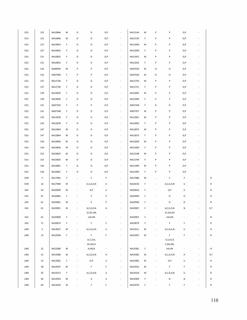
110
CEU 122 NA10846 M O O O,P -‐ NA12144 M P P O,P -‐
CEU 122 NA10846 M O O O,P -‐ NA12145 F P P O,P -‐
CEU 127 NA10854 F O O O,P -‐ NA11839 M P P O,P -‐
CEU 127 NA10854 F O O O,P -‐ NA11840 F P P O,P -‐
CEU 131 NA10855 F O O O,P -‐ NA11831 M P P O,P -‐
CEU 131 NA10855 F O O O,P -‐ NA11832 F P P O,P -‐
CEU 132 NA06994 M P P O,P -‐ NA07029 M O O O,P -‐
CEU 132 NA07000 F P P O,P -‐ NA07029 M O O O,P -‐
CEU 137 NA12740 F O O O,P -‐ NA12750 M P P O,P -‐
CEU 137 NA12740 F O O O,P -‐ NA12751 F P P O,P -‐
CEU 139 NA10839 F O O O,P -‐ NA12005 M P P O,P -‐
CEU 139 NA10839 F O O O,P -‐ NA12006 F P P O,P -‐
CEU 141 NA07345 F P P O,P -‐ NA07348 F O O O,P -‐
CEU 141 NA07348 F O O O,P -‐ NA07357 M P P O,P -‐
CEU 143 NA12878 F O O O,P -‐ NA12891 M P P O,P -‐
CEU 143 NA12878 F O O O,P -‐ NA12892 F P P O,P -‐
CEU 147 NA12864 M O O O,P -‐ NA12872 M P P O,P -‐
CEU 147 NA12864 M O O O,P -‐ NA12873 F P P O,P -‐
CEU 150 NA10856 M O O O,P -‐ NA11829 M P P O,P -‐
CEU 150 NA10856 M O O O,P -‐ NA11830 F P P O,P -‐
CEU 152 NA10835 M O O O,P -‐ NA12248 M P P O,P -‐
CEU 152 NA10835 M O O O,P -‐ NA12249 F P P O,P -‐
CEU 156 NA10861 F O O O,P -‐ NA11994 M P P O,P -‐
CEU 156 NA10861 F O O O,P -‐ NA11995 F P P O,P -‐
CHD 2 NA17981 F -‐ F F -‐ NA17986 M -‐ F F -‐ R
CHD 16 NA17980 M -‐ A,C,G,H,N U -‐ NA18150 F -‐ A,C,G,H,N U -‐ R
GIH 54 NA20909 M -‐ O,P U -‐ NA20910 F -‐ O,P U -‐ R
GIH 61 NA20882 F -‐ P P -‐ NA20900 F -‐ O O -‐ R
GIH 61 NA20891 M -‐ P P -‐ NA20900 F -‐ O O -‐ R
GIH 61 NA20891 M -‐ A,C,G,H,N A -‐ NA20907 F -‐ A,C,G,H,N N -‐ R,?
GIH 61 NA20900 F -‐
1C,GC,GN
,HA,HN -‐ -‐ NA20907 F -‐
1C,GA,GG
,HA,HN -‐ -‐ N
GIH 71 NA20874 F -‐ F F -‐ NA20879 F -‐ F F -‐ R
LWK 3 NA19027 M -‐ A,C,G,H,N U -‐ NA19311 M -‐ A,C,G,H,N U -‐ R
LWK 13 NA19396 F -‐ F F -‐ NA19397 M -‐ F F -‐ R
LWK 22 NA19380 M -‐
1C,C,GA,
GC,GG,H
A,HN,N -‐ -‐ NA19381 F -‐
1C,A,G,G
C,GG,GN,
HA,HN -‐ -‐ N
LWK 22 NA19380 M -‐ A,C,G,H,N H -‐ NA19382 M -‐ A,C,G,H,N H -‐ R,?
LWK 22 NA19381 F -‐ O,P U -‐ NA19382 M -‐ O,P U -‐ R
LWK 38 NA19347 M -‐ F F -‐ NA19352 M -‐ F F -‐ R
LWK 45 NA19313 F -‐ A,C,G,H,N U -‐ NA19334 M -‐ A,C,G,H,N U -‐ R
LWK 60 NA19443 M -‐ A A -‐ NA19469 F -‐ N N -‐ R
LWK 60 NA19443 M -‐ F F -‐ NA19470 F -‐ F F -‐ R
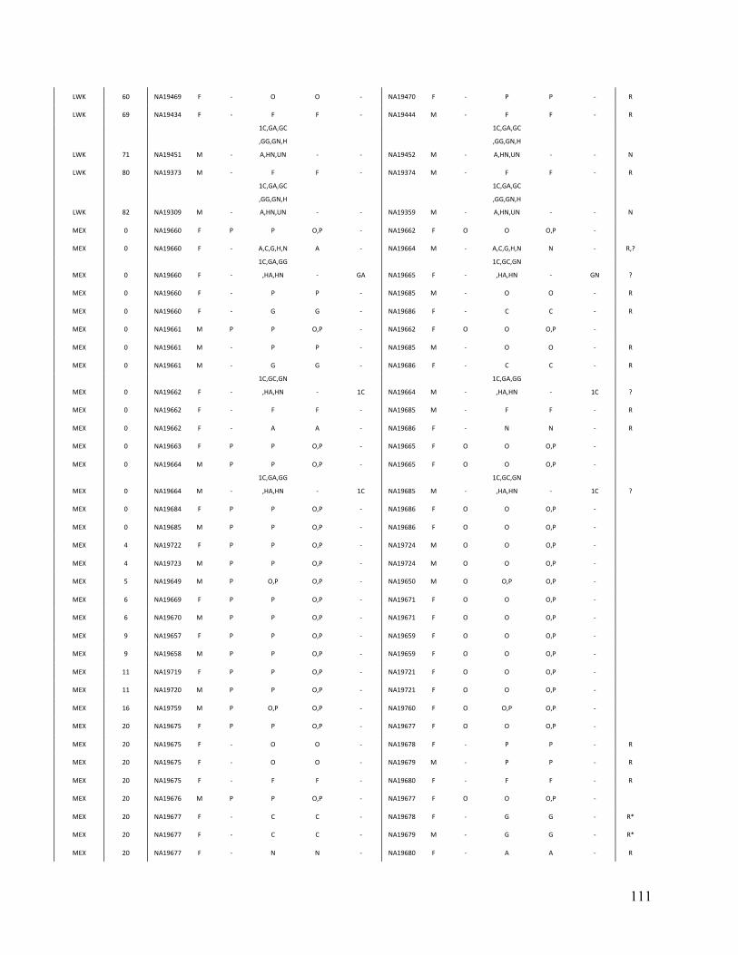
111
LWK 60 NA19469 F -‐ O O -‐ NA19470 F -‐ P P -‐ R
LWK 69 NA19434 F -‐ F F -‐ NA19444 M -‐ F F -‐ R
LWK 71 NA19451 M -‐
1C,GA,GC
,GG,GN,H
A,HN,UN -‐ -‐ NA19452 M -‐
1C,GA,GC
,GG,GN,H
A,HN,UN -‐ -‐ N
LWK 80 NA19373 M -‐ F F -‐ NA19374 M -‐ F F -‐ R
LWK 82 NA19309 M -‐
1C,GA,GC
,GG,GN,H
A,HN,UN -‐ -‐ NA19359 M -‐
1C,GA,GC
,GG,GN,H
A,HN,UN -‐ -‐ N
MEX 0 NA19660 F P P O,P -‐ NA19662 F O O O,P -‐
MEX 0 NA19660 F -‐ A,C,G,H,N A -‐ NA19664 M -‐ A,C,G,H,N N -‐ R,?
MEX 0 NA19660 F -‐
1C,GA,GG
,HA,HN -‐ GA NA19665 F -‐
1C,GC,GN
,HA,HN -‐ GN ?
MEX 0 NA19660 F -‐ P P -‐ NA19685 M -‐ O O -‐ R
MEX 0 NA19660 F -‐ G G -‐ NA19686 F -‐ C C -‐ R
MEX 0 NA19661 M P P O,P -‐ NA19662 F O O O,P -‐
MEX 0 NA19661 M -‐ P P -‐ NA19685 M -‐ O O -‐ R
MEX 0 NA19661 M -‐ G G -‐ NA19686 F -‐ C C -‐ R
MEX 0 NA19662 F -‐
1C,GC,GN
,HA,HN -‐ 1C NA19664 M -‐
1C,GA,GG
,HA,HN -‐ 1C ?
MEX 0 NA19662 F -‐ F F -‐ NA19685 M -‐ F F -‐ R
MEX 0 NA19662 F -‐ A A -‐ NA19686 F -‐ N N -‐ R
MEX 0 NA19663 F P P O,P -‐ NA19665 F O O O,P -‐
MEX 0 NA19664 M P P O,P -‐ NA19665 F O O O,P -‐
MEX 0 NA19664 M -‐
1C,GA,GG
,HA,HN -‐ 1C NA19685 M -‐
1C,GC,GN
,HA,HN -‐ 1C ?
MEX 0 NA19684 F P P O,P -‐ NA19686 F O O O,P -‐
MEX 0 NA19685 M P P O,P -‐ NA19686 F O O O,P -‐
MEX 4 NA19722 F P P O,P -‐ NA19724 M O O O,P -‐
MEX 4 NA19723 M P P O,P -‐ NA19724 M O O O,P -‐
MEX 5 NA19649 M P O,P O,P -‐ NA19650 M O O,P O,P -‐
MEX 6 NA19669 F P P O,P -‐ NA19671 F O O O,P -‐
MEX 6 NA19670 M P P O,P -‐ NA19671 F O O O,P -‐
MEX 9 NA19657 F P P O,P -‐ NA19659 F O O O,P -‐
MEX 9 NA19658 M P P O,P -‐ NA19659 F O O O,P -‐
MEX 11 NA19719 F P P O,P -‐ NA19721 F O O O,P -‐
MEX 11 NA19720 M P P O,P -‐ NA19721 F O O O,P -‐
MEX 16 NA19759 M P O,P O,P -‐ NA19760 F O O,P O,P -‐
MEX 20 NA19675 F P P O,P -‐ NA19677 F O O O,P -‐
MEX 20 NA19675 F -‐ O O -‐ NA19678 F -‐ P P -‐ R
MEX 20 NA19675 F -‐ O O -‐ NA19679 M -‐ P P -‐ R
MEX 20 NA19675 F -‐ F F -‐ NA19680 F -‐ F F -‐ R
MEX 20 NA19676 M P P O,P -‐ NA19677 F O O O,P -‐
MEX 20 NA19677 F -‐ C C -‐ NA19678 F -‐ G G -‐ R*
MEX 20 NA19677 F -‐ C C -‐ NA19679 M -‐ G G -‐ R*
MEX 20 NA19677 F -‐ N N -‐ NA19680 F -‐ A A -‐ R
112
MEX 20 NA19678 F P P O,P -‐ NA19680 F O O O,P -‐
MEX 20 NA19679 M P P O,P -‐ NA19680 F O O O,P -‐
MEX 23 NA19651 F P P O,P -‐ NA19653 F O O O,P -‐
MEX 23 NA19652 M P P O,P -‐ NA19653 F O O O,P -‐
MEX 26 NA19725 F P P O,P -‐ NA19727 M O O O,P -‐
MEX 26 NA19726 M P P O,P -‐ NA19727 M O O O,P -‐
MEX 28 NA19755 F P P O,P -‐ NA19757 M O O O,P -‐
MEX 28 NA19756 M P P O,P -‐ NA19757 M O O O,P -‐
MEX 32 NA19773 F P P O,P -‐ NA19775 F O O O,P -‐
MEX 32 NA19774 M P P O,P -‐ NA19775 F O O O,P -‐
MEX 35 NA19776 F P P O,P -‐ NA19778 M O O O,P -‐
MEX 35 NA19777 M P P O,P -‐ NA19778 M O O O,P -‐
MEX 38 NA19782 F P P O,P -‐ NA19784 M O O O,P -‐
MEX 38 NA19783 M P P O,P -‐ NA19784 M O O O,P -‐
MEX 45 NA19779 F P P O,P -‐ NA19781 F O O O,P -‐
MEX 45 NA19780 M P P O,P -‐ NA19781 F O O O,P -‐
MEX 54 NA19681 F P P O,P -‐ NA19683 F O O O,P -‐
MEX 54 NA19682 M P P O,P -‐ NA19683 F O O O,P -‐
MEX 55 NA19746 F P P O,P -‐ NA19748 F O O O,P -‐
MEX 55 NA19747 M P P O,P -‐ NA19748 F O O O,P -‐
MEX 59 NA19716 F P O,P O,P -‐ NA19718 F O O,P O,P -‐
MEX 61 NA19794 F P P O,P -‐ NA19796 M O O O,P -‐
MEX 61 NA19795 M P P O,P -‐ NA19796 M O O O,P -‐
MEX 63 NA19654 F P O,P O,P -‐ NA19656 F O O,P O,P -‐
MEX 64 NA19749 F P P O,P -‐ NA19751 M O O O,P -‐
MEX 64 NA19750 M P P O,P -‐ NA19751 M O O O,P -‐
MEX 67 NA19761 F P P O,P -‐ NA19763 F O O O,P -‐
MEX 67 NA19762 M P P O,P -‐ NA19763 F O O O,P -‐
MEX 69 NA19770 F P P O,P -‐ NA19772 M O O O,P -‐
MEX 69 NA19771 M P P O,P -‐ NA19772 M O O O,P -‐
MEX 73 NA19788 F P P O,P -‐ NA19790 F O O O,P -‐
MEX 73 NA19789 M P P O,P -‐ NA19790 F O O O,P -‐
MKK 8 NA21399 M P P O,P -‐ NA21401 M O O O,P -‐
MKK 8 NA21399 M -‐ F F -‐ NA21402 M -‐ F F -‐ R
MKK 8 NA21399 M -‐ A A -‐ NA21404 F -‐ N N -‐ R*
MKK 8 NA21399 M -‐ F F -‐ NA21405 M -‐ F F -‐ R
MKK 8 NA21400 F P P O,P -‐ NA21401 M O O O,P -‐
MKK 8 NA21401 M -‐ N N -‐ NA21402 M -‐ A A -‐ R*
MKK 8 NA21401 M -‐ 1C -‐ -‐ NA21404 F -‐ 1C -‐ -‐ N
MKK 8 NA21401 M -‐ N N -‐ NA21405 M -‐ A A -‐ R
MKK 8 NA21402 M P P O,P -‐ NA21404 F O O O,P -‐
MKK 8 NA21402 M -‐ F F -‐ NA21405 M -‐ F F -‐ R
MKK 8 NA21403 F P P O,P -‐ NA21404 F O O O,P -‐
113
MKK 8 NA21404 F -‐ N N -‐ NA21405 M -‐ A A -‐ R*
MKK 16 NA21716 M P P O,P -‐ NA21718 M O O O,P -‐
MKK 16 NA21716 M -‐ A,C,G,H,N A -‐ NA21741 M -‐ A,C,G,H,N N -‐ R,?
MKK 16 NA21717 F P P O,P -‐ NA21718 M O O O,P -‐
MKK 16 NA21718 M -‐
1C,GC,GN
,HA,HN -‐ -‐ NA21741 M -‐
1C,GA,GG
,HA,HN -‐ -‐ N
MKK 25 NA21723 F -‐ A,C,G,H,N H -‐ NA21733 F -‐ A,C,G,H,N H -‐ R,?
MKK 26 NA21307 M P P O,P -‐ NA21309 F O O O,P -‐
MKK 26 NA21307 M -‐ A,C,G,H,N A -‐ NA21616 M -‐ A,C,G,H,N N -‐ R,?
MKK 26 NA21308 F P P O,P -‐ NA21309 F O O O,P -‐
MKK 26 NA21308 F -‐ A,C,G,H,N A -‐ NA21379 F -‐ A,C,G,H,N N -‐ R,?
MKK 26 NA21308 F -‐ A,C,G,H,N H -‐ NA21517 F -‐ A,C,G,H,N H -‐ R,?
MKK 26 NA21309 F -‐
1C,GC,GN
,HA,HN -‐ -‐ NA21379 F -‐
1C,GA,GG
,HA,HN -‐ -‐ N
MKK 26 NA21309 F -‐
1C,GC,GN
,HA,HN -‐ -‐ NA21517 F -‐
1C,GA,GG
,HA,HN -‐ -‐ N
MKK 26 NA21309 F -‐
1C,GC,GN
,HA,HN -‐ -‐ NA21616 M -‐
1C,GA,GG
,HA,HN -‐ -‐ N
MKK 26 NA21379 F -‐ 1C,UN -‐ -‐ NA21517 F -‐ 1C,UN -‐ -‐ N
MKK 31 NA21357 F -‐ F F -‐ NA21509 M -‐ F F -‐ R
MKK 40 NA21381 M P P O,P -‐ NA21383 M O O O,P -‐
MKK 40 NA21382 F P P O,P -‐ NA21383 M O O O,P -‐
MKK 40 NA21382 F -‐
1C,GA,GG
,HA,HN -‐ -‐ NA21384 M -‐
1C,GC,GN
,HA,HN -‐ -‐ N
MKK 40 NA21382 F -‐ A,C,G,H,N N -‐ NA21387 M -‐ A,C,G,H,N A -‐ R,?
MKK 40 NA21382 F -‐
1C,GA,GG
,HA,HN -‐ -‐ NA21389 M -‐
1C,GC,GN
,HA,HN -‐ -‐ N
MKK 40 NA21383 M -‐
1C,GC,GN
,HA,HN -‐ -‐ NA21387 M -‐
1C,GA,GG
,HA,HN -‐ -‐ N
MKK 40 NA21384 M P P O,P -‐ NA21386 F O O O,P -‐
MKK 40 NA21384 M -‐ O O -‐ NA21387 M -‐ P P -‐ R
MKK 40 NA21384 M -‐ O O -‐ NA21388 F -‐ P P -‐ R
MKK 40 NA21384 M -‐ F F -‐ NA21389 M -‐ F F -‐ R
MKK 40 NA21385 F P P O,P -‐ NA21386 F O O O,P -‐
MKK 40 NA21386 F -‐ C C -‐ NA21387 M -‐ G G -‐ R
MKK 40 NA21386 F -‐ C C -‐ NA21388 F -‐ G G -‐ R
MKK 40 NA21386 F -‐ N N -‐ NA21389 M -‐ A A -‐ R*
MKK 40 NA21387 M P P O,P -‐ NA21389 M O O O,P -‐
MKK 40 NA21388 F P P O,P -‐ NA21389 M O O O,P -‐
MKK 43 NA21521 M -‐ A,C,G,H,N U -‐ NA21599 M -‐ A,C,G,H,N U -‐ R
MKK 43 NA21521 M -‐
1C,GA,GG
,HA,HN -‐ -‐ NA21601 F -‐
1C,GC,GN
,HA,HN -‐ -‐ N
MKK 43 NA21599 M P P O,P -‐ NA21601 F O O O,P -‐
MKK 43 NA21600 F P P O,P -‐ NA21601 F O O O,P -‐
MKK 57 NA21620 F -‐ A,C,G,H,N U -‐ NA21719 M -‐ A,C,G,H,N U -‐ R
MKK 68 NA21574 F -‐ O,P U -‐ NA21575 M -‐ O,P U -‐ R
MKK 101 NA21457 F -‐ F F -‐ NA21683 F -‐ F F -‐ R
114
MKK 105 NA21363 F -‐ O,P U -‐ NA21415 F -‐ O,P U -‐ R
MKK 114 NA21440 M P P O,P -‐ NA21442 M O O O,P -‐
MKK 114 NA21441 F P P O,P -‐ NA21442 M O O O,P -‐
MKK 115 NA21359 M P P O,P -‐ NA21361 F O O O,P -‐
MKK 115 NA21360 F P P O,P -‐ NA21361 F O O O,P -‐
MKK 119 NA21391 F -‐ A,C,G,H,N H -‐ NA21421 F -‐ A,C,G,H,N H -‐ R,?
MKK 119 NA21391 F -‐ 1C,UN -‐ -‐ NA21478 M -‐ 1C,UN -‐ -‐ N
MKK 119 NA21391 F -‐
1C,GA,GC
,GG,GN,H
A,HN -‐ -‐ NA21485 M -‐
1C,GA,GC
,GG,GN,H
A,HN -‐ -‐ N
MKK 119 NA21391 F -‐
1C,GA,GC
,GG,GN,H
A,HN,UN -‐ -‐ NA21488 M -‐
1C,GA,GC
,GG,GN,H
A,HN,UN -‐ -‐ N
MKK 119 NA21421 F -‐ 1C,UN -‐ -‐ NA21478 M -‐ 1C,UN -‐ -‐ N
MKK 119 NA21421 F -‐ A,C,G,H,N U -‐ NA21485 M -‐ A,C,G,H,N U -‐ R
MKK 119 NA21421 F -‐
1C,GA,GG
,HA,HN -‐ -‐ NA21487 F -‐
1C,GC,GN
,HA,HN -‐ -‐ N
MKK 119 NA21421 F -‐ 1C,UN -‐ -‐ NA21488 M -‐ 1C,UN -‐ -‐ N
MKK 119 NA21475 M P P O,P -‐ NA21477 M O O O,P -‐
MKK 119 NA21475 M -‐
1C,GC,GN
,HA,HN -‐ -‐ NA21478 M -‐
1C,GA,GG
,HA,HN -‐ -‐ N
MKK 119 NA21475 M -‐
1C,GC,GN
,HA,HN -‐ -‐ NA21485 M -‐
1C,GA,GG
,HA,HN -‐ -‐ N
MKK 119 NA21475 M -‐ O O -‐ NA21488 M -‐ P P -‐ R
MKK 119 NA21475 M -‐ O O -‐ NA21489 F -‐ P P -‐ R
MKK 119 NA21475 M -‐ F F -‐ NA21490 M -‐ F F -‐ R
MKK 119 NA21476 F P P O,P -‐ NA21477 M O O O,P -‐
MKK 119 NA21477 M -‐ C C -‐ NA21488 M -‐ G G -‐ R
MKK 119 NA21477 M -‐ C C -‐ NA21489 F -‐ G G -‐ R
MKK 119 NA21477 M -‐ N N -‐ NA21490 M -‐ A A -‐ R
MKK 119 NA21478 M P P O,P -‐ NA21480 F O O O,P -‐
MKK 119 NA21478 M -‐
1C,GA,GC
,GG,GN,H
A,HN,UN -‐ -‐ NA21485 M -‐
1C,GA,GC
,GG,GN,H
A,HN,UN -‐ -‐ N
MKK 119 NA21478 M -‐ GC,UN -‐ -‐ NA21487 F -‐ GG,UN -‐ -‐ N
MKK 119 NA21478 M -‐ A,C,G,H,N U -‐ NA21488 M -‐ A,C,G,H,N U -‐ R
MKK 119 NA21478 M -‐
1C,GA,GG
,HA,HN -‐ -‐ NA21490 M -‐
1C,GC,GN
,HA,HN -‐ -‐ N
MKK 119 NA21479 F P P O,P -‐ NA21480 F O O O,P -‐
MKK 119 NA21479 F -‐ A,C,G,H,N H -‐ NA21685 M -‐ A,C,G,H,N H -‐ R,?
MKK 119 NA21480 F -‐
1C,GC,GN
,HA,HN -‐ -‐ NA21488 M -‐
1C,GA,GG
,HA,HN -‐ -‐ N
MKK 119 NA21480 F -‐
1C,GC,GN
,HA,HN -‐ -‐ NA21685 M -‐
1C,GA,GG
,HA,HN -‐ -‐ N
MKK 119 NA21485 M P P O,P -‐ NA21487 F O O O,P -‐
MKK 119 NA21485 M -‐ A,C,G,H,N U -‐ NA21488 M -‐ A,C,G,H,N U -‐ R
MKK 119 NA21485 M -‐
1C,GA,GG
,HA,HN -‐ -‐ NA21490 M -‐
1C,GC,GN
,HA,HN -‐ -‐ N
MKK 119 NA21486 F P P O,P -‐ NA21487 F O O O,P -‐

115
MKK 119 NA21487 F -‐
1C,GC,GN
,HA,HN -‐ -‐ NA21488 M -‐
1C,GA,GG
,HA,HN -‐ -‐ N
MKK 119 NA21488 M P P O,P -‐ NA21490 M O O O,P -‐
MKK 119 NA21489 F P P O,P -‐ NA21490 M O O O,P -‐
MKK 125 NA21352 M -‐ A,C,G,H,N U -‐ NA21414 M -‐ A,C,G,H,N U -‐ R
MKK 125 NA21352 M -‐
1C,GA,GG
,HA,HN -‐ -‐ NA21527 M -‐
1C,GC,GN
,HA,HN -‐ -‐ N
MKK 125 NA21352 M -‐ A,C,G,H,N U -‐ NA21583 M -‐ A,C,G,H,N U -‐ R
MKK 125 NA21414 M -‐ 1C,UN -‐ -‐ NA21583 M -‐ 1C,UN -‐ -‐ N
MKK 125 NA21526 F P P O,P -‐ NA21527 M O O O,P -‐
MKK 125 NA21527 M O O O,P -‐ NA21583 M P P O,P -‐
MKK 131 NA21300 F -‐
1C,GA,GG
,HA,HN,U
N -‐ -‐ NA21312 M -‐
1C,GC,GN
,HA,HN,U
N -‐ -‐ N
MKK 131 NA21300 F -‐
1C,GA,GG
,HA,HN,U
N -‐ -‐ NA21370 M -‐
1C,GC,GN
,HA,HN,U
N -‐ -‐ N
MKK 131 NA21300 F -‐ 1C,UN -‐ -‐ NA21435 M -‐ 1C,UN -‐ -‐ N
MKK 131 NA21300 F -‐ A,G,H,N G -‐ NA21520 M -‐ A,C,H,N C -‐ R*,?
MKK 131 NA21300 F -‐ A,G,H,N G -‐ NA21613 F -‐ A,C,H,N C -‐ R,?
MKK 131 NA21300 F -‐ A,C,G,H,N H -‐ NA21617 F -‐ A,C,G,H,N H -‐ R,?
MKK 131 NA21300 F -‐ 1C,UN -‐ -‐ NA21647 M -‐ 1C,UN -‐ -‐ N
MKK 131 NA21300 F -‐ 1C,UN -‐ -‐ NA21686 F -‐ 1C,UN -‐ -‐ N
MKK 131 NA21300 F -‐ 1C,UN -‐ -‐ NA21825 F -‐ 1C,UN -‐ -‐ N
MKK 131 NA21301 M P P O,P -‐ NA21302 F O O O,P -‐
MKK 131 NA21301 M -‐ F F -‐ NA21344 M -‐ F F -‐ R
MKK 131 NA21301 M -‐ A A -‐ NA21366 M -‐ N N -‐ R*
MKK 131 NA21302 F O O O,P -‐ NA21303 F P P O,P -‐
MKK 131 NA21302 F -‐ N N -‐ NA21344 M -‐ A A -‐ R*
MKK 131 NA21302 F -‐ 1C -‐ -‐ NA21366 M -‐ 1C -‐ -‐ N
MKK 131 NA21311 M -‐ G,H H -‐ NA21312 M -‐ C,H H -‐ R*,?
MKK 131 NA21311 M -‐ GG,HA -‐ -‐ NA21313 M -‐ GC,HN -‐ -‐ N
MKK 131 NA21311 M -‐ O,P O -‐ NA21314 M -‐ O,P P -‐ R,?
MKK 131 NA21311 M -‐ G,H C -‐ NA21320 F -‐ C,H G -‐ R,?
MKK 131 NA21311 M -‐
1C,GC,GG
,GN,HA,H
N,UN -‐ -‐ NA21367 M -‐
1C,GA,GC
,GG,HA,H
N,UN -‐ -‐ N
MKK 131 NA21311 M -‐ 1C,UN -‐ -‐ NA21424 F -‐ 1C,UN -‐ -‐ N
MKK 131 NA21311 M -‐ 1C,UN -‐ -‐ NA21596 M -‐ 1C,UN -‐ -‐ N
MKK 131 NA21312 M P P O,P -‐ NA21313 M O O O,P -‐
MKK 131 NA21312 M -‐ O O -‐ NA21314 M -‐ P P -‐ R
MKK 131 NA21312 M -‐ G,H C -‐ NA21320 F -‐ C,H G -‐ R*,?
MKK 131 NA21312 M -‐
1C,GC,GN
,HA,HN -‐ -‐ NA21367 M -‐
1C,GA,GG
,HA,HN -‐ -‐ N
MKK 131 NA21312 M -‐ H U -‐ NA21370 M -‐ H U -‐ R,P
MKK 131 NA21312 M -‐
1C,GA,GC
,GG,GN,H
A,HN,UN -‐ -‐ NA21423 M -‐
1C,GA,GC
,GG,GN,H
A,HN,UN -‐ -‐ N

116
MKK 131 NA21312 M -‐ 1C,UN -‐ -‐ NA21424 F -‐ 1C,UN -‐ -‐ N
MKK 131 NA21312 M -‐ 1C,UN -‐ -‐ NA21447 M -‐ 1C,UN -‐ -‐ N
MKK 131 NA21312 M -‐
1C,GC,GN
,HA,HN,U
N -‐ -‐ NA21520 M -‐
1C,GA,GG
,HA,HN,U
N -‐ -‐ N
MKK 131 NA21312 M -‐ 1C,UN -‐ -‐ NA21596 M -‐ 1C,UN -‐ -‐ N
MKK 131 NA21312 M -‐
1C,GC,GN
,HA,HN,U
N -‐ -‐ NA21613 F -‐
1C,GA,GG
,HA,HN,U
N -‐ -‐ N
MKK 131 NA21312 M -‐ C,H,N U -‐ NA21617 F -‐ A,G,H U -‐ R,P
MKK 131 NA21313 M -‐ C C -‐ NA21314 M -‐ G G -‐ R
MKK 131 NA21313 M -‐ HA,HN -‐ -‐ NA21320 F -‐ HA,HN -‐ -‐ N
MKK 131 NA21313 M O O O,P -‐ NA21362 F P P O,P -‐
MKK 131 NA21313 M -‐ HN -‐ -‐ NA21370 M -‐ HA -‐ -‐ N
MKK 131 NA21313 M -‐
1C,GC,GN
,HA,HN -‐ -‐ NA21438 F -‐
1C,GA,GG
,HA,HN -‐ -‐ N
MKK 131 NA21313 M -‐
GC,GN,H
N -‐ -‐ NA21617 F -‐
GA,GG,H
A -‐ -‐ N
MKK 131 NA21314 M -‐ P O -‐ NA21320 F -‐ O P -‐ R
MKK 131 NA21314 M -‐ A,C,G,H,N H -‐ NA21367 M -‐ A,C,G,H,N H -‐ R,?
MKK 131 NA21314 M -‐ 1C,UN -‐ -‐ NA21378 M -‐ 1C,UN -‐ -‐ N
MKK 131 NA21314 M -‐
1C,GA,GC
,GG,GN,H
A,HN,UN -‐ -‐ NA21423 M -‐
1C,GA,GC
,GG,GN,H
A,HN,UN -‐ -‐ N
MKK 131 NA21314 M -‐ 1C,UN -‐ -‐ NA21424 F -‐ 1C,UN -‐ -‐ N
MKK 131 NA21314 M -‐ GC,UN -‐ -‐ NA21425 F -‐ GG,UN -‐ -‐ N
MKK 131 NA21314 M -‐ 1C,UN -‐ -‐ NA21447 M -‐ 1C,UN -‐ -‐ N
MKK 131 NA21314 M -‐ 1C,UN -‐ -‐ NA21493 F -‐ 1C,UN -‐ -‐ N
MKK 131 NA21314 M -‐ 1C,UN -‐ -‐ NA21596 M -‐ 1C,UN -‐ -‐ N
MKK 131 NA21316 M P P O,P -‐ NA21317 M O O O,P -‐
MKK 131 NA21316 M -‐ F F -‐ NA21318 M -‐ F F -‐ R
MKK 131 NA21316 M -‐ A,C,H,N C -‐ NA21519 M -‐ A,G,H,N G -‐ R,?
MKK 131 NA21316 M -‐ 1C,UN -‐ -‐ NA21619 M -‐ 1C,UN -‐ -‐ N
MKK 131 NA21316 M -‐
1C,GA,GC
,GG,GN,H
A,HN,UN -‐ -‐ NA21635 F -‐
1C,GA,GC
,GG,GN,H
A,HN,UN -‐ -‐ N
MKK 131 NA21316 M -‐
1C,GA,GC
,GG,GN,H
A,HN,UN -‐ -‐ NA21678 M -‐
1C,GA,GC
,GG,GN,H
A,HN,UN -‐ -‐ N
MKK 131 NA21317 M -‐ N N -‐ NA21318 M -‐ A A -‐ R
MKK 131 NA21317 M -‐
1C,GC,GN
,HN -‐ -‐ NA21519 M -‐
1C,GA,GG
,HA -‐ -‐ N
MKK 131 NA21317 M O O O,P -‐ NA21580 F P P O,P -‐
MKK 131 NA21318 M -‐ A,C,H,N C -‐ NA21519 M -‐ A,G,H,N G -‐ R,?
MKK 131 NA21318 M -‐ 1C,UN -‐ -‐ NA21619 M -‐ 1C,UN -‐ -‐ N
MKK 131 NA21318 M -‐
1C,GA,GC
,GG,GN,H
A,HN,UN -‐ -‐ NA21635 F -‐
1C,GA,GC
,GG,GN,H
A,HN,UN -‐ -‐ N
117
MKK 131 NA21318 M -‐
1C,GA,GC
,GG,GN,H
A,HN,UN -‐ -‐ NA21678 M -‐
1C,GA,GC
,GG,GN,H
A,HN,UN -‐ -‐ N
MKK 131 NA21320 F -‐ H,N H -‐ NA21365 F -‐ A,H H -‐ R,?
MKK 131 NA21320 F -‐ 1C,HA -‐ -‐ NA21366 M -‐ 1C,HN -‐ -‐ N
MKK 131 NA21320 F -‐
1C,GC,GN
,HA,HN -‐ -‐ NA21367 M -‐
1C,GA,GG
,HA,HN -‐ -‐ N
MKK 131 NA21320 F -‐
1C,GA,GC
,GG,GN,H
A,HN,UN -‐ -‐ NA21423 M -‐
1C,GA,GC
,GG,GN,H
A,HN,UN -‐ -‐ N
MKK 131 NA21320 F -‐ 1C,UN -‐ -‐ NA21424 F -‐ 1C,UN -‐ -‐ N
MKK 131 NA21320 F -‐ 1C,UN -‐ -‐ NA21447 M -‐ 1C,UN -‐ -‐ N
MKK 131 NA21320 F -‐ H,N H -‐ NA21523 M -‐ A,H H -‐ R*,?
MKK 131 NA21320 F -‐ 1C,HA -‐ -‐ NA21525 M -‐ 1C,HN -‐ -‐ N
MKK 131 NA21320 F -‐ 1C,UN -‐ -‐ NA21596 M -‐ 1C,UN -‐ -‐ N
MKK 131 NA21344 M P P O,P -‐ NA21366 M O O O,P -‐
MKK 131 NA21362 F -‐ A,C,G,H,N H -‐ NA21438 F -‐ A,C,G,H,N H -‐ R*,?
MKK 131 NA21362 F -‐
1C,GA,GG
,HA,HN -‐ -‐ NA21439 M -‐
1C,GC,GN
,HA,HN -‐ -‐ N
MKK 131 NA21362 F -‐
1C,GN,HA
,HN,UN -‐ -‐ NA21528 M -‐
1C,GA,HA
,HN,UN -‐ -‐ N
MKK 131 NA21362 F -‐
1C,GN,HA
,HN,UN -‐ -‐ NA21587 M -‐
1C,GA,HA
,HN,UN -‐ -‐ N
MKK 131 NA21365 F P P O,P -‐ NA21366 M O O O,P -‐
MKK 131 NA21365 F -‐ F F -‐ NA21523 M -‐ F F -‐ R
MKK 131 NA21365 F -‐ A A -‐ NA21525 M -‐ N N -‐ R*
MKK 131 NA21366 M -‐ N N -‐ NA21523 M -‐ A A -‐ R
MKK 131 NA21366 M -‐ 1C -‐ -‐ NA21525 M -‐ 1C -‐ -‐ N
MKK 131 NA21367 M -‐
1C,GA,GN
,HA,HN,U
N -‐ -‐ NA21378 M -‐
1C,GA,GN
,HA,HN,U
N -‐ -‐ N
MKK 131 NA21367 M -‐ 1C,UN -‐ -‐ NA21423 M -‐ 1C,UN -‐ -‐ N
MKK 131 NA21367 M -‐ 1C,UN -‐ -‐ NA21424 F -‐ 1C,UN -‐ -‐ N
MKK 131 NA21367 M -‐ 1C,UN -‐ -‐ NA21447 M -‐ 1C,UN -‐ -‐ N
MKK 131 NA21367 M -‐
1C,GA,GN
,HA,HN,U
N -‐ -‐ NA21493 F -‐
1C,GA,GN
,HA,HN,U
N -‐ -‐ N
MKK 131 NA21367 M -‐ 1C,GC,UN -‐ -‐ NA21596 M -‐
1C,GG,U
N -‐ -‐ N
MKK 131 NA21370 M -‐ H H -‐ NA21494 F -‐ H H -‐ R
MKK 131 NA21370 M -‐
1C,GC,GN
,HA,HN,U
N -‐ -‐ NA21520 M -‐
1C,GA,GG
,HA,HN,U
N -‐ -‐ N
MKK 131 NA21370 M -‐ O O -‐ NA21522 M -‐ P P -‐ R
MKK 131 NA21370 M -‐
1C,GN,HA
,HN -‐ -‐ NA21528 M -‐
1C,GA,HA
,HN -‐ -‐ N
MKK 131 NA21370 M -‐
1C,GN,HA
,HN -‐ -‐ NA21587 M -‐
1C,GA,HA
,HN -‐ -‐ N
MKK 131 NA21370 M -‐
1C,GC,GN
,HA,HN,U
N -‐ -‐ NA21613 F -‐
1C,GA,GG
,HA,HN,U
N -‐ -‐ N

118
MKK 131 NA21370 M -‐ C,H,N U -‐ NA21617 F -‐ A,G,H U -‐ R,P
MKK 131 NA21370 M -‐ C,H H -‐ NA21682 M -‐ G,H H -‐ R,?
MKK 131 NA21378 M -‐ A,C,H,N C -‐ NA21448 M -‐ A,G,H,N G -‐ R,?
MKK 131 NA21378 M -‐ A,C,H,N U -‐ NA21453 M -‐ A,G,H,N U -‐ R§,P
MKK 131 NA21378 M -‐
1C,GA,HA
,HN -‐ -‐ NA21455 F -‐
1C,GN,HA
,HN -‐ -‐ N
MKK 131 NA21378 M -‐ F F -‐ NA21493 F -‐ F F -‐ R
MKK 131 NA21378 M -‐ A A -‐ NA21494 F -‐ N N -‐ R*
MKK 131 NA21423 M P P O,P -‐ NA21425 F O O O,P -‐
MKK 131 NA21423 M -‐
1C,GA,GG
,HA,HN -‐ -‐ NA21439 M -‐
1C,GC,GN
,HA,HN -‐ -‐ N
MKK 131 NA21423 M -‐ A,C,G,H,N A -‐ NA21447 M -‐ A,C,G,H,N N -‐ R,?
MKK 131 NA21424 F P P O,P -‐ NA21425 F O O O,P -‐
MKK 131 NA21424 F -‐ F F -‐ NA21596 M -‐ F F -‐ R
MKK 131 NA21425 F -‐
1C,GC,GN
,HA,HN -‐ -‐ NA21447 M -‐
1C,GA,GG
,HA,HN -‐ -‐ N
MKK 131 NA21425 F -‐ N N -‐ NA21596 M -‐ A A -‐ R
MKK 131 NA21435 M -‐ 1C,UN -‐ -‐ NA21520 M -‐ 1C,UN -‐ -‐ N
MKK 131 NA21435 M -‐ 1C,UN -‐ -‐ NA21613 F -‐ 1C,UN -‐ -‐ N
MKK 131 NA21435 M -‐
1C,GA,GC
,GG,GN,H
A,HN,UN -‐ -‐ NA21617 F -‐
1C,GA,GC
,GG,GN,H
A,HN,UN -‐ -‐ N
MKK 131 NA21435 M -‐ A,C,G,H,N U -‐ NA21634 M -‐ A,C,G,H,N U -‐ R
MKK 131 NA21435 M -‐
1C,GA,GG
,HA,HN -‐ -‐ NA21636 F -‐
1C,GC,GN
,HA,HN -‐ -‐ N
MKK 131 NA21435 M -‐
1C,A,C,G,
GA,GC,G
G,GN,H,H
A,HN,N U -‐ NA21647 M -‐
1C,A,C,G,
GA,GC,G
G,GN,H,H
A,HN,N U -‐ R
MKK 131 NA21435 M -‐
1C,GA,GG
,HA,HN,U
N -‐ -‐ NA21648 M -‐
1C,GC,GN
,HA,HN,U
N -‐ -‐ N
MKK 131 NA21435 M -‐ A,C,G,H,N H -‐ NA21825 F -‐ A,C,G,H,N H -‐ R,?
MKK 131 NA21438 F P P O,P -‐ NA21439 M O O O,P -‐
MKK 131 NA21439 M O O O,P -‐ NA21447 M P P O,P -‐
MKK 131 NA21448 M -‐ A,C,G,H,N H -‐ NA21453 M -‐ A,C,G,H,N H -‐ R,?
MKK 131 NA21448 M -‐
1C,GA,GG
,HA,HN -‐ -‐ NA21455 F -‐
1C,GC,GN
,HA,HN -‐ -‐ N
MKK 131 NA21448 M -‐ A,G,H,N G -‐ NA21493 F -‐ A,C,H,N C -‐ R,?
MKK 131 NA21448 M -‐
1C,GA,GG
,HA -‐ -‐ NA21494 F -‐
1C,GC,GN
,HN -‐ -‐ N
MKK 131 NA21453 M P P O,P -‐ NA21455 F O O O,P -‐
MKK 131 NA21453 M -‐ A,G,H,N U -‐ NA21493 F -‐ A,C,H,N U -‐ R§,P
MKK 131 NA21453 M -‐
1C,GA,GG
,HA -‐ -‐ NA21494 F -‐
1C,GC,GN
,HN -‐ -‐ N
MKK 131 NA21454 F P P O,P -‐ NA21455 F O O O,P -‐
MKK 131 NA21455 F -‐
1C,GN,HA
,HN -‐ -‐ NA21493 F -‐
1C,GA,HA
,HN -‐ -‐ N
MKK 131 NA21493 F P P O,P -‐ NA21494 F O O O,P -‐
MKK 131 NA21494 F O O O,P -‐ NA21522 M P P O,P -‐
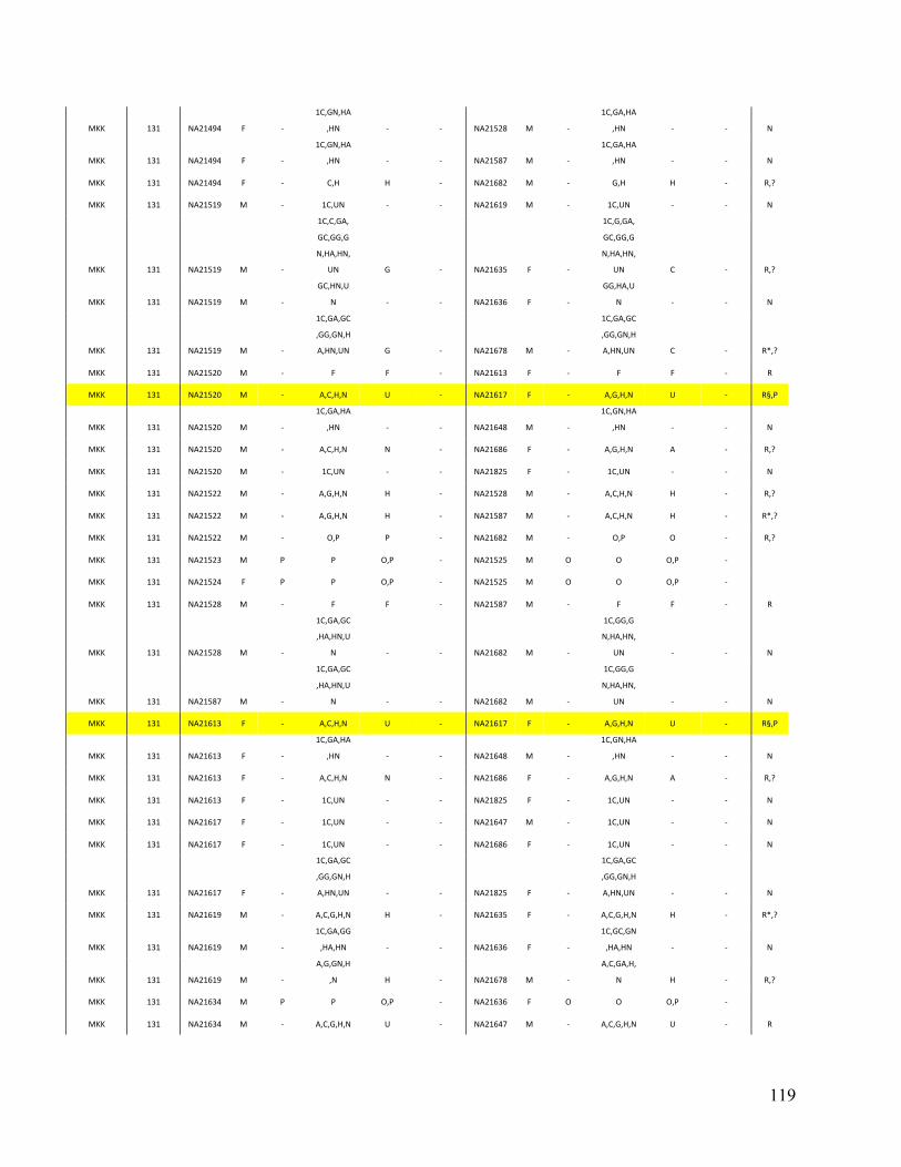
119
MKK 131 NA21494 F -‐
1C,GN,HA
,HN -‐ -‐ NA21528 M -‐
1C,GA,HA
,HN -‐ -‐ N
MKK 131 NA21494 F -‐
1C,GN,HA
,HN -‐ -‐ NA21587 M -‐
1C,GA,HA
,HN -‐ -‐ N
MKK 131 NA21494 F -‐ C,H H -‐ NA21682 M -‐ G,H H -‐ R,?
MKK 131 NA21519 M -‐ 1C,UN -‐ -‐ NA21619 M -‐ 1C,UN -‐ -‐ N
MKK 131 NA21519 M -‐
1C,C,GA,
GC,GG,G
N,HA,HN,
UN G -‐ NA21635 F -‐
1C,G,GA,
GC,GG,G
N,HA,HN,
UN C -‐ R,?
MKK 131 NA21519 M -‐
GC,HN,U
N -‐ -‐ NA21636 F -‐
GG,HA,U
N -‐ -‐ N
MKK 131 NA21519 M -‐
1C,GA,GC
,GG,GN,H
A,HN,UN G -‐ NA21678 M -‐
1C,GA,GC
,GG,GN,H
A,HN,UN C -‐ R*,?
MKK 131 NA21520 M -‐ F F -‐ NA21613 F -‐ F F -‐ R
MKK 131 NA21520 M -‐ A,C,H,N U -‐ NA21617 F -‐ A,G,H,N U -‐ R§,P
MKK 131 NA21520 M -‐
1C,GA,HA
,HN -‐ -‐ NA21648 M -‐
1C,GN,HA
,HN -‐ -‐ N
MKK 131 NA21520 M -‐ A,C,H,N N -‐ NA21686 F -‐ A,G,H,N A -‐ R,?
MKK 131 NA21520 M -‐ 1C,UN -‐ -‐ NA21825 F -‐ 1C,UN -‐ -‐ N
MKK 131 NA21522 M -‐ A,G,H,N H -‐ NA21528 M -‐ A,C,H,N H -‐ R,?
MKK 131 NA21522 M -‐ A,G,H,N H -‐ NA21587 M -‐ A,C,H,N H -‐ R*,?
MKK 131 NA21522 M -‐ O,P P -‐ NA21682 M -‐ O,P O -‐ R,?
MKK 131 NA21523 M P P O,P -‐ NA21525 M O O O,P -‐
MKK 131 NA21524 F P P O,P -‐ NA21525 M O O O,P -‐
MKK 131 NA21528 M -‐ F F -‐ NA21587 M -‐ F F -‐ R
MKK 131 NA21528 M -‐
1C,GA,GC
,HA,HN,U
N -‐ -‐ NA21682 M -‐
1C,GG,G
N,HA,HN,
UN -‐ -‐ N
MKK 131 NA21587 M -‐
1C,GA,GC
,HA,HN,U
N -‐ -‐ NA21682 M -‐
1C,GG,G
N,HA,HN,
UN -‐ -‐ N
MKK 131 NA21613 F -‐ A,C,H,N U -‐ NA21617 F -‐ A,G,H,N U -‐ R§,P
MKK 131 NA21613 F -‐
1C,GA,HA
,HN -‐ -‐ NA21648 M -‐
1C,GN,HA
,HN -‐ -‐ N
MKK 131 NA21613 F -‐ A,C,H,N N -‐ NA21686 F -‐ A,G,H,N A -‐ R,?
MKK 131 NA21613 F -‐ 1C,UN -‐ -‐ NA21825 F -‐ 1C,UN -‐ -‐ N
MKK 131 NA21617 F -‐ 1C,UN -‐ -‐ NA21647 M -‐ 1C,UN -‐ -‐ N
MKK 131 NA21617 F -‐ 1C,UN -‐ -‐ NA21686 F -‐ 1C,UN -‐ -‐ N
MKK 131 NA21617 F -‐
1C,GA,GC
,GG,GN,H
A,HN,UN -‐ -‐ NA21825 F -‐
1C,GA,GC
,GG,GN,H
A,HN,UN -‐ -‐ N
MKK 131 NA21619 M -‐ A,C,G,H,N H -‐ NA21635 F -‐ A,C,G,H,N H -‐ R*,?
MKK 131 NA21619 M -‐
1C,GA,GG
,HA,HN -‐ -‐ NA21636 F -‐
1C,GC,GN
,HA,HN -‐ -‐ N
MKK 131 NA21619 M -‐
A,G,GN,H
,N H -‐ NA21678 M -‐
A,C,GA,H,
N H -‐ R,?
MKK 131 NA21634 M P P O,P -‐ NA21636 F O O O,P -‐
MKK 131 NA21634 M -‐ A,C,G,H,N U -‐ NA21647 M -‐ A,C,G,H,N U -‐ R
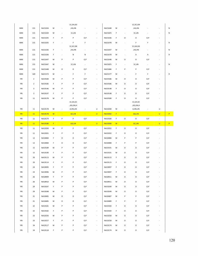
120
MKK 131 NA21634 M -‐
1C,GA,GG
,HA,HN -‐ -‐ NA21648 M -‐
1C,GC,GN
,HA,HN -‐ -‐ N
MKK 131 NA21634 M -‐ 1C,UN -‐ -‐ NA21825 F -‐ 1C,UN -‐ -‐ N
MKK 131 NA21635 F P P O,P -‐ NA21636 F O O O,P -‐
MKK 131 NA21635 F -‐ F F -‐ NA21678 M -‐ F F -‐ R
MKK 131 NA21636 F -‐
1C,GC,GN
,HA,HN -‐ -‐ NA21647 M -‐
1C,GA,GG
,HA,HN -‐ -‐ N
MKK 131 NA21636 F -‐ N N -‐ NA21678 M -‐ A A -‐ R
MKK 131 NA21647 M P P O,P -‐ NA21648 M O O O,P -‐
MKK 131 NA21647 M -‐ 1C,UN -‐ -‐ NA21825 F -‐ 1C,UN -‐ -‐ N
MKK 131 NA21648 M O O O,P -‐ NA21686 F P P O,P -‐
MKK 169 NA21573 M -‐ F F -‐ NA21577 M -‐ F F -‐ R
YRI 2 NA19184 M P P O,P -‐ NA19186 M O O O,P -‐
YRI 2 NA19185 F P P O,P -‐ NA19186 M O O O,P -‐
YRI 3 NA19146 M P P O,P -‐ NA19148 F O O O,P -‐
YRI 3 NA19147 F P P O,P -‐ NA19148 F O O O,P -‐
YRI 11 NA19178 M P P O,P -‐ NA19180 F O O O,P -‐
YRI 11 NA19178 M -‐
1C,GA,GC
,GG,GN,H
A,HN,UN -‐ U NA19200 M -‐
1C,GA,GC
,GG,GN,H
A,HN,UN -‐ U
YRI 11 NA19178 M -‐ GC,UN -‐ U NA19202 F -‐ GG,UN -‐ U P
YRI 11 NA19179 F P P O,P -‐ NA19180 F O O O,P -‐
YRI 11 NA19180 F -‐ GG,UN -‐ U NA19200 M -‐ GC,UN -‐ U P
YRI 11 NA19200 M P P O,P -‐ NA19202 F O O O,P -‐
YRI 11 NA19201 F P P O,P -‐ NA19202 F O O O,P -‐
YRI 12 NA18484 F O O O,P -‐ NA18486 M P P O,P -‐
YRI 12 NA18484 F O O O,P -‐ NA18488 F P P O,P -‐
YRI 15 NA19189 M P P O,P -‐ NA19191 M O O O,P -‐
YRI 15 NA19190 F P P O,P -‐ NA19191 M O O O,P -‐
YRI 20 NA19113 M P P O,P -‐ NA19115 F O O O,P -‐
YRI 20 NA19114 F P P O,P -‐ NA19115 F O O O,P -‐
YRI 24 NA19095 F P P O,P -‐ NA19097 F O O O,P -‐
YRI 24 NA19096 M P P O,P -‐ NA19097 F O O O,P -‐
YRI 26 NA18909 F P P O,P -‐ NA18911 M O O O,P -‐
YRI 26 NA18910 M P P O,P -‐ NA18911 M O O O,P -‐
YRI 29 NA19247 F P P O,P -‐ NA19249 M O O O,P -‐
YRI 29 NA19248 M P P O,P -‐ NA19249 M O O O,P -‐
YRI 31 NA18485 M O O O,P -‐ NA18487 M P P O,P -‐
YRI 31 NA18485 M O O O,P -‐ NA18489 F P P O,P -‐
YRI 32 NA19181 M P P O,P -‐ NA19183 F O O O,P -‐
YRI 32 NA19182 F P P O,P -‐ NA19183 F O O O,P -‐
YRI 33 NA19256 M P P O,P -‐ NA19258 M O O O,P -‐
YRI 33 NA19257 F P P O,P -‐ NA19258 M O O O,P -‐
YRI 34 NA19117 M P P O,P -‐ NA19174 M O O O,P -‐
YRI 34 NA19118 F P P O,P -‐ NA19174 M O O O,P -‐
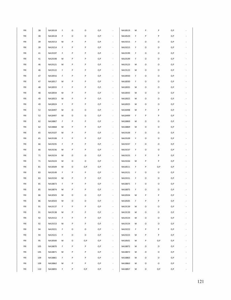
121
YRI 38 NA18518 F O O O,P -‐ NA18519 M P P O,P -‐
YRI 38 NA18518 F O O O,P -‐ NA18520 F P P O,P -‐
YRI 39 NA19213 M P P O,P -‐ NA19215 F O O O,P -‐
YRI 39 NA19214 F P P O,P -‐ NA19215 F O O O,P -‐
YRI 41 NA19197 F P P O,P -‐ NA19199 F O O O,P -‐
YRI 41 NA19198 M P P O,P -‐ NA19199 F O O O,P -‐
YRI 46 NA19121 M P P O,P -‐ NA19123 M O O O,P -‐
YRI 46 NA19122 F P P O,P -‐ NA19123 M O O O,P -‐
YRI 47 NA18916 F P P O,P -‐ NA18930 F O O O,P -‐
YRI 47 NA18917 M P P O,P -‐ NA18930 F O O O,P -‐
YRI 48 NA18933 F P P O,P -‐ NA18935 M O O O,P -‐
YRI 48 NA18934 M P P O,P -‐ NA18935 M O O O,P -‐
YRI 49 NA18923 M P P O,P -‐ NA18925 M O O O,P -‐
YRI 49 NA18924 F P P O,P -‐ NA18925 M O O O,P -‐
YRI 52 NA18497 M O O O,P -‐ NA18498 M P P O,P -‐
YRI 52 NA18497 M O O O,P -‐ NA18499 F P P O,P -‐
YRI 62 NA18867 F P P O,P -‐ NA18869 M O O O,P -‐
YRI 62 NA18868 M P P O,P -‐ NA18869 M O O O,P -‐
YRI 65 NA19107 M P P O,P -‐ NA19109 F O O O,P -‐
YRI 65 NA19108 F P P O,P -‐ NA19109 F O O O,P -‐
YRI 66 NA19235 F P P O,P -‐ NA19237 F O O O,P -‐
YRI 66 NA19236 M P P O,P -‐ NA19237 F O O O,P -‐
YRI 71 NA19224 M O O O,P -‐ NA19225 F P P O,P -‐
YRI 71 NA19224 M O O O,P -‐ NA19226 M P P O,P -‐
YRI 81 NA18509 M O O,P O,P -‐ NA18511 F P O,P O,P -‐
YRI 83 NA19149 F P P O,P -‐ NA19151 F O O O,P -‐
YRI 83 NA19150 M P P O,P -‐ NA19151 F O O O,P -‐
YRI 85 NA18873 F P P O,P -‐ NA18875 F O O O,P -‐
YRI 85 NA18874 M P P O,P -‐ NA18875 F O O O,P -‐
YRI 86 NA18503 M O O O,P -‐ NA18504 M P P O,P -‐
YRI 86 NA18503 M O O O,P -‐ NA18505 F P P O,P -‐
YRI 91 NA19137 F P P O,P -‐ NA19139 M O O O,P -‐
YRI 91 NA19138 M P P O,P -‐ NA19139 M O O O,P -‐
YRI 92 NA19152 F P P O,P -‐ NA19154 M O O O,P -‐
YRI 92 NA19153 M P P O,P -‐ NA19154 M O O O,P -‐
YRI 94 NA19221 F O O O,P -‐ NA19222 F P P O,P -‐
YRI 94 NA19221 F O O O,P -‐ NA19223 M P P O,P -‐
YRI 95 NA18500 M O O,P O,P -‐ NA18501 M P O,P O,P -‐
YRI 105 NA18870 F P P O,P -‐ NA18872 M O O O,P -‐
YRI 105 NA18871 M P P O,P -‐ NA18872 M O O O,P -‐
YRI 109 NA18861 F P P O,P -‐ NA18863 M O O O,P -‐
YRI 109 NA18862 M P P O,P -‐ NA18863 M O O O,P -‐
YRI 110 NA18855 F P O,P O,P -‐ NA18857 M O O,P O,P -‐

122
YRI 115 NA19171 M P P O,P -‐ NA19173 M O O O,P -‐
YRI 115 NA19172 F P P O,P -‐ NA19173 M O O O,P -‐
YRI 117 NA18515 M O O O,P -‐ NA18516 M P P O,P -‐
YRI 117 NA18515 M O O O,P -‐ NA18517 F P P O,P -‐
YRI 122 NA18912 F P P O,P -‐ NA18914 M O O O,P -‐
YRI 122 NA18913 M P P O,P -‐ NA18914 M O O O,P -‐
YRI 122 NA18913 M -‐ O,P O,P -‐ NA19238 F -‐ O,P O,P -‐
YRI 122 NA18913 M -‐ G,H H -‐ NA19240 F -‐ C,H H -‐ R,?
YRI 122 NA18914 M -‐ C,H C -‐ NA19238 F -‐ G,H G -‐ R,?
YRI 122 NA18914 M -‐ HA,HN -‐ HN NA19240 F -‐ HA,HN -‐ HA ?
YRI 122 NA19238 F P P O,P -‐ NA19240 F O O O,P -‐
YRI 122 NA19239 M P P O,P -‐ NA19240 F O O O,P -‐
YRI 131 NA19209 F P P O,P -‐ NA19211 M O O O,P -‐
YRI 131 NA19210 M P P O,P -‐ NA19211 M O O O,P -‐
YRI 133 NA18506 M O O O,P -‐ NA18507 M P P O,P -‐
YRI 133 NA18506 M O O O,P -‐ NA18508 F P P O,P -‐
YRI 134 NA19159 F P P O,P -‐ NA19161 M O O O,P -‐
YRI 134 NA19160 M P P O,P -‐ NA19161 M O O O,P -‐
YRI 141 NA18858 F P P O,P -‐ NA18860 M O O O,P -‐
YRI 141 NA18859 M P P O,P -‐ NA18860 M O O O,P -‐
YRI 149 NA19127 F P P O,P -‐ NA19129 F O O O,P -‐
YRI 149 NA19128 M P P O,P -‐ NA19129 F O O O,P -‐
YRI 150 NA19130 M P P O,P -‐ NA19132 F O O O,P -‐
YRI 150 NA19130 M -‐ A,C,G,H,N AV -‐ NA19192 M -‐ A,C,G,H,N AV -‐ ?
YRI 150 NA19130 M -‐
1C,GA,GG
,HA,HN -‐ 1C NA19194 M -‐
1C,GC,GN
,HA,HN -‐ 1C ?
YRI 150 NA19131 F P P O,P -‐ NA19132 F O O O,P -‐
YRI 150 NA19132 F -‐
1C,GC,GN
,HA,HN -‐ GN NA19192 M -‐
1C,GA,GG
,HA,HN -‐ GA ?
YRI 150 NA19192 M P P O,P -‐ NA19194 M O O O,P -‐
YRI 150 NA19193 F P P O,P -‐ NA19194 M O O O,P -‐
YRI 152 NA19116 F P P O,P -‐ NA19120 M O O O,P -‐
YRI 152 NA19119 M P P O,P -‐ NA19120 M O O O,P -‐
YRI 155 NA19093 F P O,P O,P -‐ NA19094 F O O,P O,P -‐
YRI 157 NA18852 F P P O,P -‐ NA18854 M O O O,P -‐
YRI 157 NA18853 M P P O,P -‐ NA18854 M O O O,P -‐
YRI 160 NA19140 F P P O,P -‐ NA19142 M O O O,P -‐
YRI 160 NA19141 M P P O,P -‐ NA19142 M O O O,P -‐
YRI 164 NA19206 F P P O,P -‐ NA19208 M O O O,P -‐
YRI 164 NA19207 M P P O,P -‐ NA19208 M O O O,P -‐
YRI 165 NA19101 M P P O,P -‐ NA19103 M O O O,P -‐
YRI 165 NA19102 F P P O,P -‐ NA19103 M O O O,P -‐
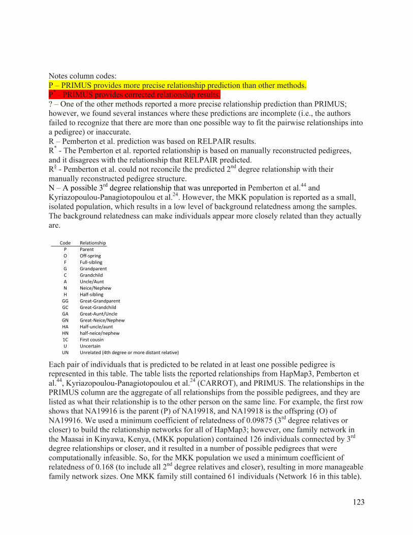
123
Notes column codes: P – PRIMUS provides more precise relationship prediction than other methods. P* - PRIMUS provides corrected relationship results. ? – One of the other methods reported a more precise relationship prediction than PRIMUS; however, we found several instances where these predictions are incomplete (i.e., the authors failed to recognize that there are more than one possible way to fit the pairwise relationships into a pedigree) or inaccurate. R – Pemberton et al. prediction was based on RELPAIR results. R* - The Pemberton et al. reported relationship is based on manually reconstructed pedigrees, and it disagrees with the relationship that RELPAIR predicted. R§ - Pemberton et al. could not reconcile the predicted 2nd degree relationship with their manually reconstructed pedigree structure. N – A possible 3rd degree relationship that was unreported in Pemberton et al.44 and Kyriazopoulou-Panagiotopoulou et al.24. However, the MKK population is reported as a small, isolated population, which results in a low level of background relatedness among the samples. The background relatedness can make individuals appear more closely related than they actually are.
Each pair of individuals that is predicted to be related in at least one possible pedigree is represented in this table. The table lists the reported relationships from HapMap3, Pemberton et al.44, Kyriazopoulou-Panagiotopoulou et al.24 (CARROT), and PRIMUS. The relationships in the PRIMUS column are the aggregate of all relationships from the possible pedigrees, and they are listed as what their relationship is to the other person on the same line. For example, the first row shows that NA19916 is the parent (P) of NA19918, and NA19918 is the offspring (O) of NA19916. We used a minimum coefficient of relatedness of 0.09875 (3rd degree relatives or closer) to build the relationship networks for all of HapMap3; however, one family network in the Maasai in Kinyawa, Kenya, (MKK population) contained 126 individuals connected by 3rd degree relationships or closer, and it resulted in a number of possible pedigrees that were computationally infeasible. So, for the MKK population we used a minimum coefficient of relatedness of 0.168 (to include all 2nd degree relatives and closer), resulting in more manageable family network sizes. One MKK family still contained 61 individuals (Network 16 in this table).
YRI 14 NA18518 F O O PO C NA18520 F P P PO CYRI 15 NA19213 M P P PO C NA19215 F O O PO CYRI 15 NA19214 F P P PO C NA19215 F O O PO CYRI 16 NA19197 F P P PO C NA19199 F O O PO CYRI 16 NA19198 M P P PO C NA19199 F O O PO CYRI 17 NA19121 M P P PO C NA19123 M O O PO CYRI 17 NA19122 F P P PO C NA19123 M O O PO CYRI 18 NA18916 F P P PO C NA18930 F O O PO CYRI 18 NA18917 M P P PO C NA18930 F O O PO CYRI 19 NA18933 F P P PO C NA18935 M O O PO CYRI 19 NA18934 M P P PO C NA18935 M O O PO CYRI 20 NA18923 M P P PO C NA18925 M O O PO CYRI 20 NA18924 F P P PO C NA18925 M O O PO CYRI 21 NA18497 M O O PO C NA18498 M P P PO CYRI 21 NA18497 M O O PO C NA18499 F P P PO CYRI 22 NA18867 F P P PO C NA18869 M O O PO CYRI 22 NA18868 M P P PO C NA18869 M O O PO CYRI 23 NA19107 M P P PO C NA19109 F O O PO CYRI 23 NA19108 F P P PO C NA19109 F O O PO CYRI 24 NA19235 F P P PO C NA19237 F O O PO CYRI 24 NA19236 M P P PO C NA19237 F O O PO CYRI 25 NA19224 M O O PO C NA19225 F P P PO CYRI 25 NA19224 M O O PO C NA19226 M P P PO CYRI 26 NA18509 M O O,P PO C NA18511 F P O,P PO CYRI 27 NA19149 F P P PO C NA19151 F O O PO CYRI 27 NA19150 M P P PO C NA19151 F O O PO CYRI 28 NA18873 F P P PO C NA18875 F O O PO CYRI 28 NA18874 M P P PO C NA18875 F O O PO CYRI 29 NA18503 M O O PO C NA18504 M P P PO CYRI 29 NA18503 M O O PO C NA18505 F P P PO CYRI 30 NA19137 F P P PO C NA19139 M O O PO CYRI 30 NA19138 M P P PO C NA19139 M O O PO CYRI 31 NA19152 F P P PO C NA19154 M O O PO CYRI 31 NA19153 M P P PO C NA19154 M O O PO CYRI 32 NA19221 F O O PO C NA19222 F P P PO CYRI 32 NA19221 F O O PO C NA19223 M P P PO CYRI 33 NA18500 M O O,P PO C NA18501 M P O,P PO CYRI 34 NA18870 F P P PO C NA18872 M O O PO CYRI 34 NA18871 M P P PO C NA18872 M O O PO CYRI 35 NA18861 F P P PO C NA18863 M O O PO CYRI 35 NA18862 M P P PO C NA18863 M O O PO CYRI 36 NA18855 F P O,P PO C NA18857 M O O,P PO CYRI 37 NA19171 M P P PO C NA19173 M O O PO CYRI 37 NA19172 F P P PO C NA19173 M O O PO CYRI 38 NA18515 M O O PO C NA18516 M P P PO CYRI 38 NA18515 M O O PO C NA18517 F P P PO CYRI 39 NA18912 F P P PO C NA18914 M O O PO CYRI 39 NA18913 M P P PO C NA18914 M O O PO CYRI 39 NA18913 M C O,P PO C NA19238 F C O,P PO CYRI 39 NA18913 M C G,H H C NA19240 F C C,H H C R,OYRI 39 NA18914 M C C,H C C NA19238 F C G,H G C R,OYRI 39 NA18914 M C HA,HN C HN NA19240 F C HA,HN C HA OYRI 39 NA19238 F P P PO C NA19240 F O O PO CYRI 39 NA19239 M P P PO C NA19240 F O O PO CYRI 40 NA19209 F P P PO C NA19211 M O O PO CYRI 40 NA19210 M P P PO C NA19211 M O O PO CYRI 41 NA18506 M O O PO C NA18507 M P P PO CYRI 41 NA18506 M O O PO C NA18508 F P P PO CYRI 42 NA19159 F P P PO C NA19161 M O O PO CYRI 42 NA19160 M P P PO C NA19161 M O O PO CYRI 43 NA18858 F P P PO C NA18860 M O O PO CYRI 43 NA18859 M P P PO C NA18860 M O O PO CYRI 44 NA19127 F P P PO C NA19129 F O O PO CYRI 44 NA19128 M P P PO C NA19129 F O O PO CYRI 45 NA19130 M P P PO C NA19132 F O O PO CYRI 45 NA19130 M C A,C,G,H,N AV C NA19192 M C A,C,G,H,N AV C OYRI 45 NA19130 M C 1C,GA,GG,HA,HN C 1C NA19194 M C 1C,GC,GN,HA,HN C 1C OYRI 45 NA19131 F P P PO C NA19132 F O O PO CYRI 45 NA19132 F C 1C,GC,GN,HA,HN C GN NA19192 M C 1C,GA,GG,HA,HN C GA OYRI 45 NA19192 M P P PO C NA19194 M O O PO CYRI 45 NA19193 F P P PO C NA19194 M O O PO CYRI 46 NA19116 F P P PO C NA19120 M O O PO CYRI 46 NA19119 M P P PO C NA19120 M O O PO CYRI 47 NA19093 F P O,P PO C NA19094 F O O,P PO CYRI 48 NA18852 F P P PO C NA18854 M O O PO CYRI 48 NA18853 M P P PO C NA18854 M O O PO CYRI 49 NA19140 F P P PO C NA19142 M O O PO CYRI 49 NA19141 M P P PO C NA19142 M O O PO CYRI 50 NA19206 F P P PO C NA19208 M O O PO CYRI 50 NA19207 M P P PO C NA19208 M O O PO CYRI 51 NA19101 M P P PO C NA19103 M O O PO CYRI 51 NA19102 F P P PO C NA19103 M O O PO C
Code RelationshipP ParentO OffCspringF FullCsiblingG GrandparentC GrandchildA Uncle/AuntN Neice/NephewH HalfCsiblingGG GreatCGrandparentGC GreatCGrandchildGA GreatCAunt/UncleGN GreatCNeice/NephewHA HalfCuncle/auntHN halfCneice/nephew1C First[cousinU UncertainUN Unrelated[(4th[degree[or[more[distant[relative)

124
To reconstruct this network, we broke it into nine sub-networks each containing four to eight closely related samples. We ran PRIMUS on each pair of sub-networks in order to reconstruct relationships between the sub-networks.
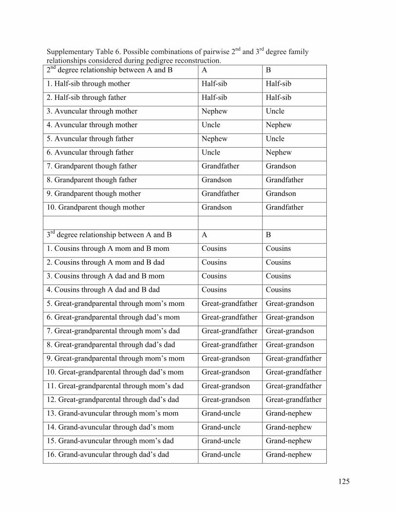
125
Supplementary Table 6. Possible combinations of pairwise 2nd and 3rd degree family relationships considered during pedigree reconstruction. 2nd degree relationship between A and B A B
1. Half-sib through mother Half-sib Half-sib
2. Half-sib through father Half-sib Half-sib
3. Avuncular through mother Nephew Uncle
4. Avuncular through mother Uncle Nephew
5. Avuncular through father Nephew Uncle
6. Avuncular through father Uncle Nephew
7. Grandparent though father Grandfather Grandson
8. Grandparent though father Grandson Grandfather
9. Grandparent though mother Grandfather Grandson
10. Grandparent though mother Grandson Grandfather
3rd degree relationship between A and B A B
1. Cousins through A mom and B mom Cousins Cousins
2. Cousins through A mom and B dad Cousins Cousins
3. Cousins through A dad and B mom Cousins Cousins
4. Cousins through A dad and B dad Cousins Cousins
5. Great-grandparental through mom’s mom Great-grandfather Great-grandson
6. Great-grandparental through dad’s mom Great-grandfather Great-grandson
7. Great-grandparental through mom’s dad Great-grandfather Great-grandson
8. Great-grandparental through dad’s dad Great-grandfather Great-grandson
9. Great-grandparental through mom’s mom Great-grandson Great-grandfather
10. Great-grandparental through dad’s mom Great-grandson Great-grandfather
11. Great-grandparental through mom’s dad Great-grandson Great-grandfather
12. Great-grandparental through dad’s dad Great-grandson Great-grandfather
13. Grand-avuncular through mom’s mom Grand-uncle Grand-nephew
14. Grand-avuncular through dad’s mom Grand-uncle Grand-nephew
15. Grand-avuncular through mom’s dad Grand-uncle Grand-nephew
16. Grand-avuncular through dad’s dad Grand-uncle Grand-nephew
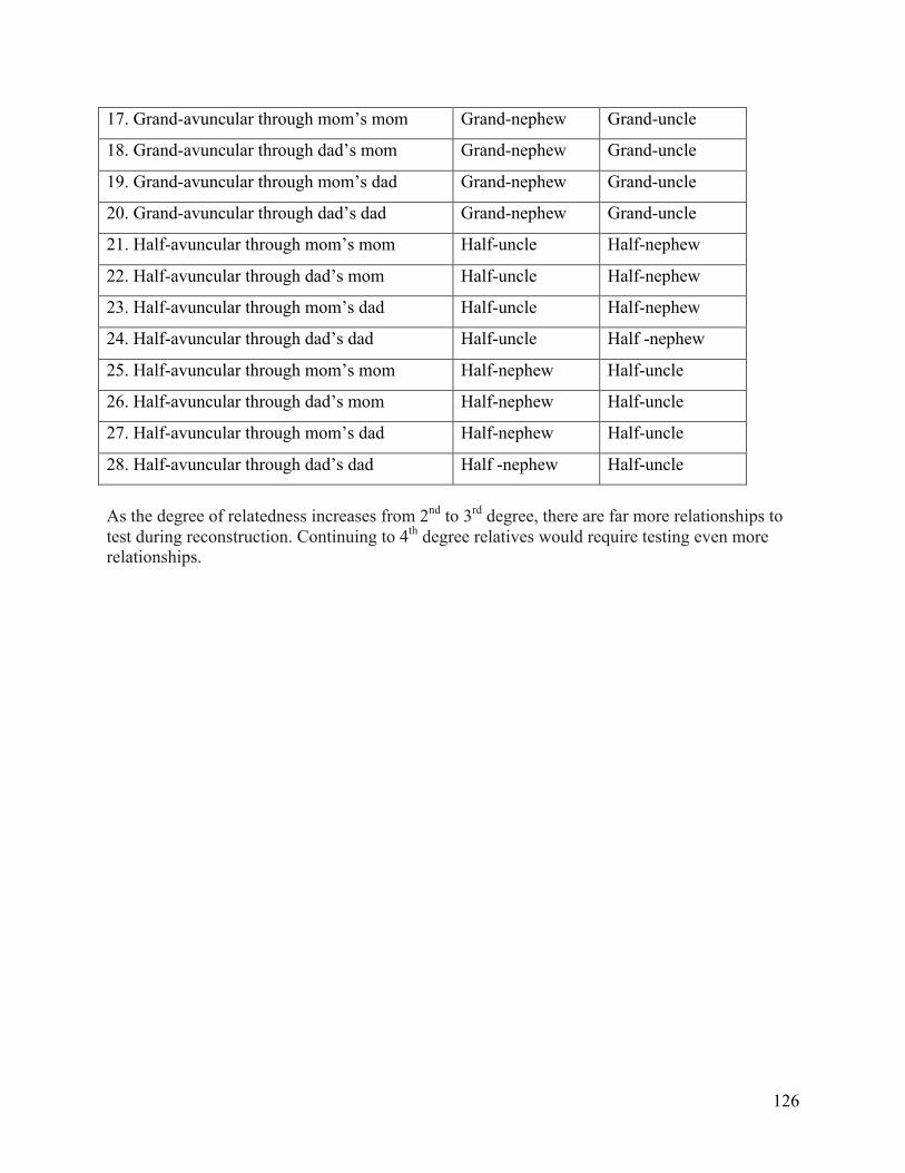
126
17. Grand-avuncular through mom’s mom Grand-nephew Grand-uncle
18. Grand-avuncular through dad’s mom Grand-nephew Grand-uncle
19. Grand-avuncular through mom’s dad Grand-nephew Grand-uncle
20. Grand-avuncular through dad’s dad Grand-nephew Grand-uncle
21. Half-avuncular through mom’s mom Half-uncle Half-nephew
22. Half-avuncular through dad’s mom Half-uncle Half-nephew
23. Half-avuncular through mom’s dad Half-uncle Half-nephew
24. Half-avuncular through dad’s dad Half-uncle Half -nephew
25. Half-avuncular through mom’s mom Half-nephew Half-uncle
26. Half-avuncular through dad’s mom Half-nephew Half-uncle
27. Half-avuncular through mom’s dad Half-nephew Half-uncle
28. Half-avuncular through dad’s dad Half -nephew Half-uncle
As the degree of relatedness increases from 2nd to 3rd degree, there are far more relationships to test during reconstruction. Continuing to 4th degree relatives would require testing even more relationships.