PRINCIPAL COMPONENT

ANALYSIS

Matrix Algebra Approach

Nomenclature

In the clustering and dimension reduction context:

• Genes are considered to be variables– Also called dimensions

– Also called components

– Also called axes

• Gene expression levels are the observed data – Also called data points

– Also called assays

– Also called samples

• Cluster Analysis (represents data points)

– To reduce the number of objects (not dimensions) by

placing them into groups

– (a cluster is the surrogate for multiple data points)

• Principle Component Analysis (reduces

dimensions)

– To reduce the number of correlated variables into a

smaller number of uncorrelated variables (reduced

dimensionality) by finding a combination of the

original variables.

(each variable is represented in a new basis, and there

may be an acceptable lower dimension of the new

basis, hence fewer variables)

INTRODUCTION

CONCEPT: Variance Information

The analysis we seek must provide the

greatest information with the least

cost/complexity

Objectives of PCA

• To reduce the dimensionality of the data set

• To identify new meaningful variables

Expression levels from genes A and B

are plotted against one another. There

are equal amounts of variance

accounted for by each gene. The

spherical shape of the data swarm

makes hidden correlations unlikely

Gene A

Ge

ne

B

Variance along axis of Gene A

Va

ria

nce a

lon

g a

xis

of

Ge

ne

B

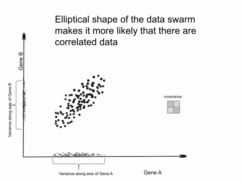
Elliptical shape of the data swarm

makes it more likely that there are

correlated data

covariance

Gene A

Ge

ne

B

Variance along axis of Gene A

Va

ria

nce a

lon

g a

xis

of

Ge

ne

B

One unique rotation angle will cause variance to maximize

on one new axis, while minimizing variance on the

orthogonal axis

covariance

Dimension Reduction

We could conceivably ignore the projection of minimal

variance on the new ordinate and consider only the

variance along the new abscissa, now the new ‘main’

axis.

Doing so would result in a single axis, having

reduced the dimension from 2 to 1, a much less

complex system

Here are gene expression data for 2 genes. The expression

levels for the first and 2nd gene are plotted against each other

0 200 400 600 800 1000 1200 14000

500

1000

1500G

en

e 1

exp

ressio

n

Gene 2 expression

Clearly the expression levels are highly correlated; gene 2

expression lends little information to what we already knew

Here is a 3-D case.

There is a great

deal of covariance

covariance

In classical statistical regression in a general linear model,

one regresses a line on the data such that the least squared

distance, in 3 dimensions, between the data points and the

line is minimized.

The regression

line does not

necessarily pass

along the

maximum

variance of all

axes

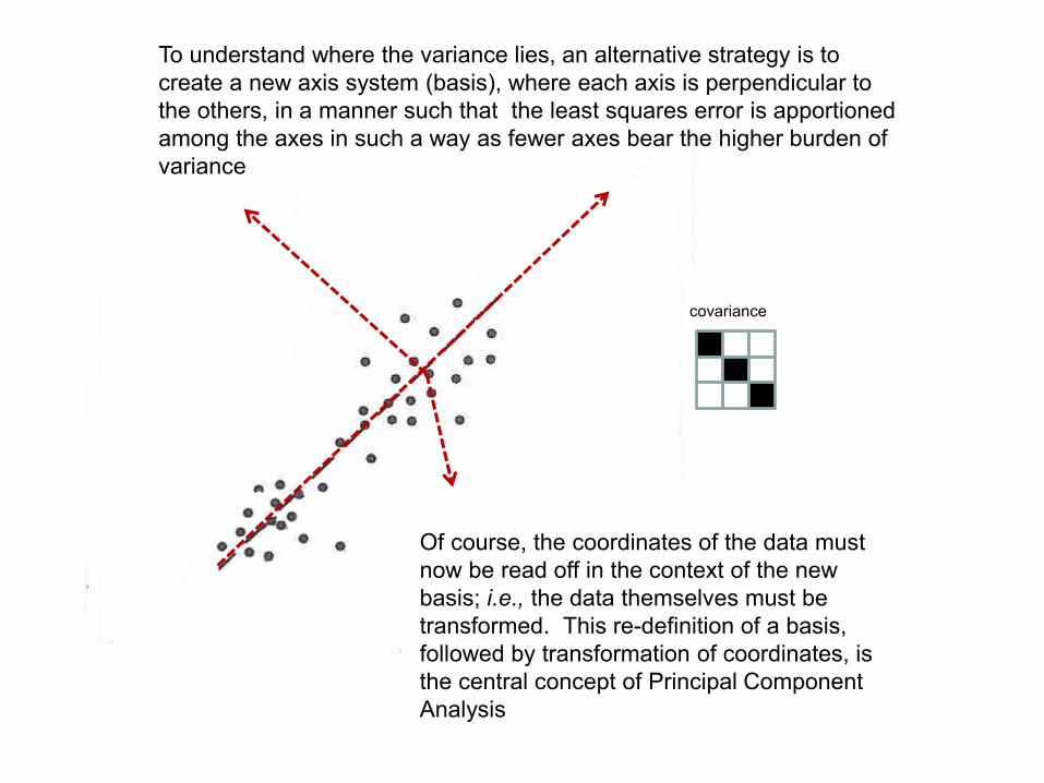
To understand where the variance lies, an alternative strategy is to

create a new axis system (basis), where each axis is perpendicular to

the others, in a manner such that the least squares error is apportioned

among the axes in such a way as fewer axes bear the higher burden of

variance

Of course, the coordinates of the data must

now be read off in the context of the new

basis; i.e., the data themselves must be

transformed. This re-definition of a basis,

followed by transformation of coordinates, is

the central concept of Principal Component

Analysis

covariance

OBJECTIVE

• Original data (vectors) lie in an N-dimensional vector space spanned by an orthonormal basis – EACH AXIS REPRESENTS A VARIABLE

• Find a new orthonormal (orthogonal and normalized) basis for the same data (vectors) – FIND A NEW SET OF VARIABLES (AXES)

• Select the new basis s.t. the variance of the projection of data on each new axis is maximized – THE NEW VARIABLES ‘EXPLAIN’ THE UNDERLYING

CORRELATIONS BETTER

– By definition of orthonormal, each of the axes is independent of the others

Finding a New Basis: A Linear Transform

• 1933 Hotelling: Principal Components

• 1946 Karhunen

• 1953 Loeve

• 1967 Lumley: Proper Orthogonal Decomposition

• 1983 Golub and Van Loen: Singular Value Decomposition

1 1 11 1 21 1 31 1 1

2 2 12 2 22 2 32 2 2

3 3 13 3 23 3 33 3 3

1 2 3

n

n

n

m m n m n m n m nn

y x v x v x v x v

y x v x v x v x v

y x v x v x v x v

y x v x v x v x v

Old axes {X1, X2, X3,…. Xn}

New axes {y1, y2, y3,…. yn}

Transformation Matrix V

The Transformation: Write every axis in the new system as a linear combination of the old axes, with every new axis orthogonal, and ||vn|| =1

K-L transformation

The Linear Transformation

• Huge amount of arithmetic to compute the

transformation head-on

• Even larger amount of arithmetic to compute

eigenvalues and eigenvectors

• Need computers!!!

– Progress mid-century arrested until computers

became available

– Using eigenstructure less efficient but more

elegant…(who cares?)

• Strategy: we need to find a linear transform that will yield a new set of axes such that the data across axes are uncorrelated (covariance=0) in the new basis.

• Approach:

In a covariance matrix, diagonal elements represent variance; off-diagonal elements represent covariance.

We want the off-diagonal elements to be zero in the covariance matrix of the transformed data (thus we will have no correlated data after transformation).

We will seek that desired structure first by recognizing that the structure we seek is a diagonal matrix, that is, a matrix whose values lie along the main diagonal and all off-diagonal elements are 0.

Finding the transformation

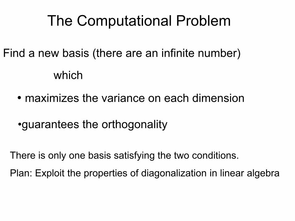
The Computational Problem

Find a new basis (there are an infinite number)

which

• maximizes the variance on each dimension

•guarantees the orthogonality

There is only one basis satisfying the two conditions.

Plan: Exploit the properties of diagonalization in linear algebra

Strategy:

•Diagonalize the correlation matrix of the raw data and define its eigenvectors to be the new ‘components’ (basis set)

•Transform the original data with our new linear transformation (the matrix of eigenvectors), yielding ‘new’ data points in each dimension

•Select from the new components those that account for the greatest variance in the problem

•Reduce the number of dimensions by eliminating those with least variance

We know:

•The covariance matrix is square, symmetric with real values*.

•The eigenvectors of a Hermitian matrix are orthogonal. As a consequence, the

eigenvectors do not project upon each other and the eigenvalues are real

•The eigenvalues tell us the variance associated with each eigenvector

We can:

•Find the eigenstructure of the covariance matrix

•There should be no (or minimal) off-diagonal entries

*This is a special case of a Hermitian matrix (square ,complex, equal to its conjugate transpose)

JUMPING TO THE ANSWER

The coefficients* to generate the first new, derived variable

(principal component) are the elements of the eigenvector*

(associated with the largest eigenvalue ) of the covariance

matrix .

Likewise for the second largest eigenvalue and its associated

eigenvector, etc.

The original data are multiplied by this eigenvector matrix,

transforming them in terms of more meaningful variables

The eigenvalues of the covariance matrix of the original data

tell us the new variance in each new axis (variable or

principal component)

*Called ‘factor loading’ in the Psychology literature

Why would all this be?

• The concept underlying this development is to

look at just one vector in the required transform

matrix, and just one element in the required new

data vector, and to maximize the variance of the

element, while at the same time making the new

vector normal.

• One this is accomplished, the process can be

generalized to all vectors in the transformation

matrix and all elements in the new data vector

The K-L Transform…..

Why would all this be?

Fact: Orthogonality implies that the off-diagonal

elements of the covariance (correlation) matrix

must be 0. If z is the standardized vector

variable,then the general linear transform is

Vz =y

where V is the coefficient matrix of the transform.

Walking through the elements of y,

• y1 is the first element of y

• v1

is the first column of matrix V

We require that:

2

1 ,

1

'

1, 1

'

1 1

1

1

N

i

i

i

y be maximizedN

y

v z

v v

Development follows Cooley,Lohnes

Variance maximization

Transformation (rotation)

Normalization

2

2 '

1 , 1

1 1

' '

1 1

1

' '

1 1

1

'

1 1

1 1

1

1

N N

i i

i i

N

i i

i

N

i i

i

yN N

N

N

v z

v z z v

v z z v

v C v C is the covariance matrix

The following is some matrix manipulation:Maximize this Maximize this

Rewrite the above

Exploit distributive property

So we have an optimization problem. Frequently, the solution to such problems is to

find the first derivative of the function (in this case, the transformation matrix) in

question, if it is differentiable.

But we have another problem: v must be normal, each vi must = 1

We need a way to solve a constrained optimization problem. In this case the

constraint is a constant.

One technique is to introduce a Lagrange multiplier

Lagrange Multipliers• Purpose: optimization of a problem with constraints, such as optimizing

f(x1,x2...) with constraints g1(x1,x2..) that are constant Strategy: Rewrite the optimization problem without constraints, using some new parameters

Minimize L(x, ) = f(x) - g1(x)

where

L(x, ) is the Lagrangian function

is the Lagrangian Multiplier

To find ,treat as a variable, finding the unconstrained minimum of L(x, ) while g1(x) = 0 is satisfied

Optimization

1. Take partial derivatives of L(x, ) with respect to xi and set

them equal to zero.

2. If there are n variables (i.e., x1, ..., xn) then you will get n + 1

simultaneous equation to solve (i.e., n variables xi and one

Lagrangian multiplier )

' '

1 1 1 1In order tomaximize where 1:v C v v v

Introduce a Lagrangian multiplier for the first v, call

it 1 (The choice of the symbol l to represent the Lagrangian

multiplier is not entirely coincidental with the same choice to represent

an eigenvalue).

Then, by adding a 0 term involving the Lagrangian,

we get a Lagrangian function in :

' '

1 1 1 1 1 1 1 v Cv v v

So…………………

This term is 0

constraint

To maximize this function, write the vector of partial

derivatives and set it to zero:

1

1 1 1

1

2 2 0

Cv vv

After simplification, we recognize that the

Lagrangian represents the eigenvalue in the

mathematical development of the eigenvalues and

eigenvectors of a matrix.

1 1 0 C I v

This only works if is differentiable

Generalize to all dimensions..

• Likewise for v2, v3 …..etc

• Each eigenvector passes from the origin

through the maximum variance remaining

in the data that are uncorrelated with the

first eigenvector

• Each eigenvalue says what that variance

is

An astounding result

We can consider the eigenstructure of the correlation matrix of our original data as the solution

The eigenvectors are our new bases vectors.

The eigenvalues tell us about the variance on each axis

The signal/noise ratio (uncorrelated/correlated) is maximized

RECIPE1. Remove the mean from the data. Even better, normalize it if

there are large fold differences among the data

2. Find the covariance matrix of the resulting adjusted data

3. Find the eigenvectors and eigenvalues of the covariance matrix

4. Sort the eigenvalue-eigenvector pairs by descending order of the eigenvalues

5. The principal components are the eigenvectors (in order of the eigenvalues) and the variance explained by each component is the eigenvalue

6. Transformed the data by the principal components

Where’s the dimension

reduction?

We have successfully transformed our vector

space from one to another.

What’s the point of that, since we were

looking for dimension reduction?

If most (for instance, 80% to 90%) of the total

population variance, for large number of

dimensions, can be attributed to the first

one, two, or three components, then these

components can “replace” the original

variables without much loss of

information.

Scree Plots show the falloff of variance in the

ordered eigenvalues

Data Reduction

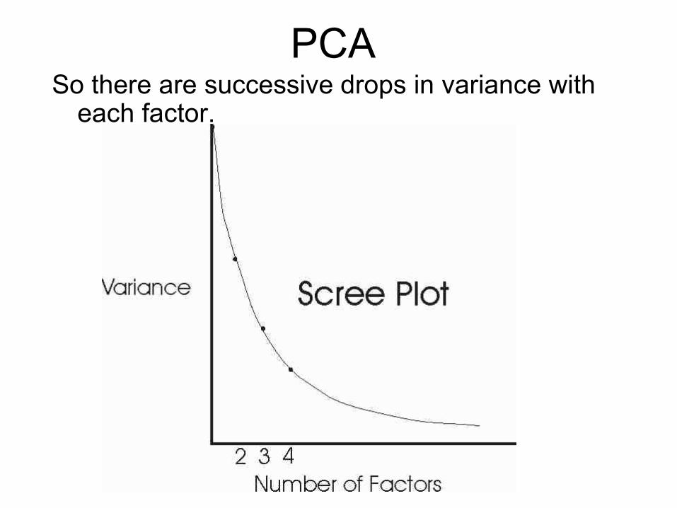
PCASo there are successive drops in variance with

each factor.

What do we have?

Usually we wish to transform our problem to

a new representation

We have new axes and new data

transformed in the context of the new

axes

Example

The Brain Tumor Gene Chip

BrainTumorChip is a matrix of artificial data from an hypothetical experiment.

There are 90 expression levels read for each of 20 genes

– The expression levels are from 18 persons

– There are 5 tissues sampled for each person• Cerebrum

• Cerebellum

• Spinal Fluid

• Meninges

• Spinal Cord

– There is a reasonable anticipation that here would be some disease specific differences among the 18 people

• 6 are normal

• 6 have meningiomas

• 6 have gliomas

Among the 20 genes, there are 5 generic types of gene action

– The genes are broadly classified as • Xf: Involved in transport

• Ra: reabsorbtion

• QW: free radical quenching

• Ta: transcriptase accelerators

• Nk: no known function

– There are 3-5 specific genes within each category

Example

The Brain Tumor Gene Chip

This is a plot of the two most highly correlated gene expression vectors in the

experiment. So nearly perfect is the correlation that the data lie along the 45 line.

The 45 line is likely the first eigenvector. The arrows show the likely direction of

the second eigenvector, orthogonal to the first eigenvector.

Gene A expression

Gene B

expre

ssio

n

This is a plot of the two least correlated gene expression vectors in the

experiment. The data do not lie along the diagonal and are not likely correlated.

The arrows suggest what will likely be the direction of the first eigenvector

Gene A expression

Ge

ne

B e

xp

ressio

n

0.8888

0.0992

0.0043

0.0029

0.0013

0.0009

0.0008

0.0007

0.0006

0.0003

0.0002

0.000

0.0000

0.0000

0.0000

0.0000

0.0000

0.0000

0.0000

0.0000

% of total variance reflected in eigenvalues

1

2

3

4

5

6

7

8

9

10

11

98.8% of variance

in the first 2

eigenvalues

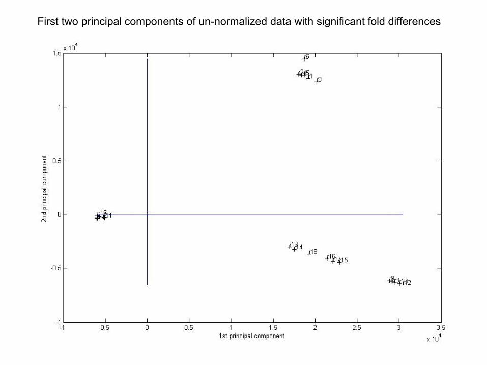
First two principal components of un-normalized data with significant fold differences

1st and 3rd principal components of un-normalized data with significant fold differences

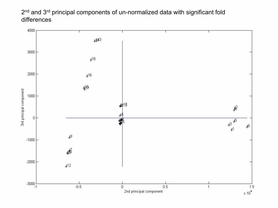
2nd and 3rd principal components of un-normalized data with significant fold

differences

Other things we may want….

• Sometimes we want to get our original data O

back, without, or, more often, with dimension

reduction

O=E-1N

Don’t forget that the mean was subtracted off the original data set,

so it must be added back

Gene A

Ge

ne

B

Reconstructed original data after removing one component

Data before PCA dimension

removal

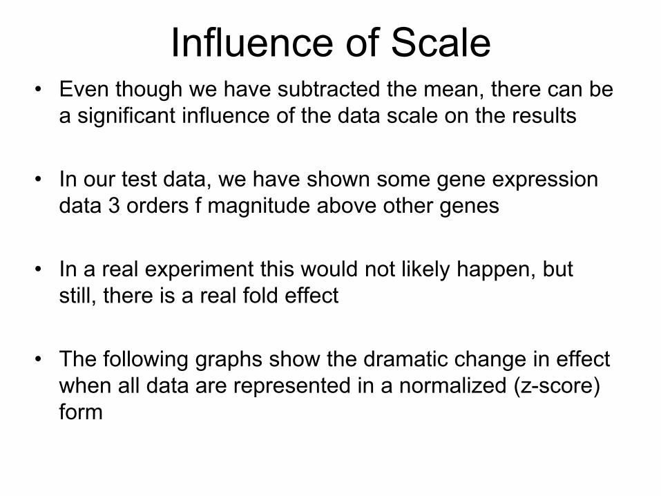
Influence of Scale• Even though we have subtracted the mean, there can be

a significant influence of the data scale on the results

• In our test data, we have shown some gene expression

data 3 orders f magnitude above other genes

• In a real experiment this would not likely happen, but

still, there is a real fold effect

• The following graphs show the dramatic change in effect

when all data are represented in a normalized (z-score)

form

0.6565

0.1396

0.1072

0.0577

0.023

0.0058

0.0052

0.0023

0.0013

0.0007

0.0003

0.0002

0.0001

0.0001

0.0000

0.0000

0.0000

0.0000

0.0000

Variance from Eigenvalues Scree Plot of Variance

1

2

3

4

5

6

7

8

9

10

11

12

13

14

96.1% of

variance

Data are represented by their z-scores- A different set of eigenvalues

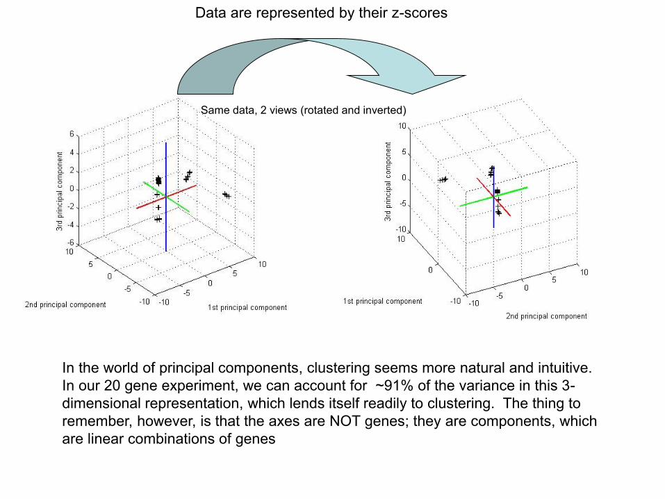
Data are represented by their z-scores

In the world of principal components, clustering seems more natural and intuitive.

In our 20 gene experiment, we can account for ~91% of the variance in this 3-

dimensional representation, which lends itself readily to clustering. The thing to

remember, however, is that the axes are NOT genes; they are components, which

are linear combinations of genes

Same data, 2 views (rotated and inverted)

Despite the fact that our goal is data reduction, not clustering, there are still natural clusters that

emerge in the lower dimensional model. It is very important to remember, however, that we are

not clustering based on gene expression levels, but rather on coordinates on the components.

meninges

Spinal fluid

Cerebellum:

normal and

meningioma

Cerebellum : glioma

1st and 2nd principal components – normalized data

Cerebellum: normal, meningioma Cerebellum: glioma

Spinal fluid

Meninges: glioma

and normal

Meninges:

meningioma

1st and 3rd principal components - normalized data

Very dense clusters

containing most of the

remaining data

2nd and 3rd principal components - normalized data

Very dense clusters

containing most of the

remaining data