principles and practice in programming languages: a ...bec/courses/csci3155-notes.pdfa body of...
TRANSCRIPT
Principles and Practice in Programming
Languages: A Project-Based Course
Bor-Yuh Evan Chang
UNIVERSITY OF COLORADO BOULDER
E-mail address: [email protected]

Draft as of August 29, 2016.
Disclaimer: This manuscript is a draft of a set of course notes for the Prin-ciples of Programming Languages at the University of Colorado Boulder.There may be typos, bugs, or inconsistencies that have yet to be resolved.

Contents
Chapter 1. Introduction and Preliminaries 11.1. Getting Your Money’s Worth 11.1.1. How? 31.2. Is a Program Executed or Evaluated? 41.2.1. Basic Values, Types, and Expressions 51.2.2. Evaluation 61.2.3. Binding Names 71.2.4. Scoping 81.2.5. Function Definitions and Tuples 101.3. Recursion, Induction, and Iteration 111.3.1. Induction: Reasoning about Recursive Programs 121.3.2. Pattern Matching 131.3.3. Function Preconditions 141.3.4. Iteration: Tail Recursion with an Accumulator 151.4. Lab 1 171.4.1. Scala Basics: Binding and Scope 171.4.2. Scala Basics: Typing 171.4.3. Run-Time Library 181.4.4. Run-Time Library: Recursion 191.4.5. Data Structures Review: Binary Search Trees 201.4.6. JavaScripty Interpreter: Numbers 22
Chapter 2. Approaching a Programming Language 252.1. Syntax: Grammars and Scoping 252.1.1. Context-Free Languages and Context-Free Grammars 262.1.1.1. Derivation of a Sentence in a Grammar. 262.1.2. Lexical and Syntactic 272.1.3. Ambiguous Grammars 282.1.4. Abstract Syntax 312.2. Structural Induction 322.2.1. Structural Induction over Lists 332.2.2. Structural Induction over Abstract Syntax Trees 362.3. Judgments 382.3.1. Example: Syntax 38
iii
iv CONTENTS
2.3.2. Derivations of Judgments 392.3.3. Structural Induction on Derivations 39
Chapter 3. Language Design and Implementation 413.1. Operational Semantics 413.1.1. Syntax: JavaScripty 413.1.2. A Big-Step Operational Semantics 423.2. Small-Step Operational Semantics 463.2.1. Evaluation Order 463.2.2. A Small-Step Operational Semantics of JAVASCRIPTY 473.2.2.1. Substitution 513.2.2.2. Multi-Step Evaluation 52
Chapter 4. Static Checking 554.1. Type Checking 554.1.1. Getting Stuck 554.1.2. Dynamic Typing 564.1.3. Static Typing 57
Bibliography 61

CHAPTER 1
Introduction and Preliminaries
1.1. Getting Your Money’s Worth
This course is about principles, concepts, and ideas that underly pro-gramming languages. But what does this statement mean?
As a student of computer science, it is completely reasonable to thinkand ask, “Why bother? I’m proficient and like programming in Ruby. Isn’tthat enough? Isn’t language choice just a matter of taste? If not, should Ibe using another language?”
Certainly, there are social factors and an aspect of personal prefer-ence that affect the programming languages that we use. But there is alsoa body of principles and mathematical theories that allow us to discussand think about languages in a rigorous manner. We study these under-pinnings because a language affects the way one approaches problemsworking in that language and affects the way one implements that lan-guage. At the end of this course, we hope that you will have grown in thefollowing ways.
You will be able to learn new languages quickly and select a suitableone for your task. This goal is very much a practical one. Languages thatare “popular” vary quickly. The TIOBE Programming Community Index1
surveys the popularity of programming languages over time. While it isjust one indicator, the take home message seems to be that a large num-ber of languages are active at any one time, and the level of activity of anylanguage varies widely over time. The “hot” languages now or the lan-guages that you study now will almost certainly not be the ones you needlater in your career.
There is a lingo for describing programming languages. The introduc-tion to any programming language is likely to include a statement thataims to succinctly captures various design choices.
Python: “Python is an interpreted, interactive, object-oriented pro-gramming language. It incorporates modules, exceptions, dy-namic typing, very high level dynamic data types, and classes.”2
1http://www.tiobe.com/content/paperinfo/tpci/, January 2012.2http://docs.python.org/faq/general#what-is-python, January 2012.
1

2 1. INTRODUCTION AND PRELIMINARIES
OCaml: OCaml offers “a power type system, equipped with para-metric polymorphism and type inference [. . . ], user-definable al-gebraic data types and pattern matching [. . . ], automatic mem-ory management [. . . ], separate compilation of stand-alone ap-plications [. . . ], a sophisticated module system [. . . ], an expres-sive object-oriented layer [. . . ], and efficient native code compil-ers.”3
Haskell: Haskell is “a polymorphically statically typed, lazy, purelyfunctional language, quite different from most other program-ming languages.”4
Scala: “Scala is a blend of object-oriented and functional program-ming concepts in a statically typed language” [3].
At this point, it is understandable if the above statements seem as if theyare written a foreign language.
You will gain new ways of viewing computation and approachingalgorithmic problems. There are fundamental models of computation orprogramming paradigms that persist (e.g., imperative programming andfunctional programming). Most general-purpose languages mix paradigmsbut generally have a bias. These biases can shape the way you approachproblems.
For natural languages, linguistic relativity, the hypothesis that the lan-guage one speaks influences the way one perceives the world, is both tan-talizing and controversial. Many have espoused this notion to program-ming languages by analogy. Setting aside the controversy and assumingat least a kernel of truth, practicing and working with different program-ming models may expose ideas in new contexts. For example, MapRe-duce is the programming model created by Google for data processingon large clusters inspired by the functional programming paradigm [1].
This course is not a survey of programming languages present andpast. We may make references to programming languages as examples ofparticular design decisions, but the goal is not to “learn” lots of languages.The analogy to natural languages is perhaps apt. It does not particularlyhelp one understand the structure of natural languages by learning to say“hello” in as many as possible.
You will gain new ways of viewing programs. The meaning of pro-gram is given by how it executes, but a program is also artifact in itselfthat has properties. What a program does or how a program executesis perhaps the primary way one views programs—a program computes
3http://caml.inria.fr/about/, January 2012.4http://www.haskell.org/haskellwiki/Introduction/, January 2012.

1.1. GETTING YOUR MONEY’S WORTH 3
something. At the same time, a program can be transformed into a differ-ent one that “behaves the same.” How do we characterize “behaves thesame”? This question is one that can be discussed using programminglanguage theory.
It is also a question of practical importance for language implementa-tion. A compiler translates a program that a human developer writes intoone a computational machine can execute. The compiler must abide bythe contract that it outputs a program for the machine that “behaves thesame” as the program written by the developer.
You will gain insight into avoiding mistakes for when you designlanguages. When (not if!) you design and implement a language, youwill avoid the mistakes of the past. You may not design a general-purposeprogramming language, but you may have a need to create a “little” con-figuration, mark-up, or layout language. “Little” languages are often cre-ated without much regard to good design because they are “little,” butthey can quickly become not so “little.”
Avoiding bad language design is tricky. Experts make mistakes, andmistakes can have long-lasting effects. Turing award winner Sir C.A.R.Hoare has called his invention of the null reference a “billion dollar mis-take” [2].
1.1.1. How? We will construct language interpreters to get experi-ence with the “guts” of programming language design and implementa-tion. The semester project will be to build and understand an interpreterfor JavaScript (or rather, a variant of it)–our example source language. Thesource language is sometimes called the object language. Along the way,we will consider the design decisions made and think about alternatives,and we will study the programming language theory that enable us toreason carefully about them. Our approach will be gradual in that we willinitially consider a small subset of our source language and then slowlygrow the aspects of the language that we consider.
Our implementation language of study will be Scala5. The implemen-tation language is sometimes called the meta language. Scala is a mod-ern, general-purpose programming language that includes many advancedideas from programming language research. In particular, we are inter-ested in it because it is especially well suited for building language tools.As quoted above, Scala “blends” concepts from object-oriented and func-tional programming [3] and in many ways tries to support each in its “na-tive environment.” Scala has also found a myriad of other applications,including being a hot language for web services right now. It is compat-ible with Java and runs on the Java Virtual Machine (JVM) and has been
5http://www.scala-lang.org/, August 2012.

4 1. INTRODUCTION AND PRELIMINARIES
applied in industrial practice by such companies as LinkedIn and Twit-ter.6
1.2. Is a Program Executed or Evaluated?
Broadly speaking, the “schism” between imperative programming andfunctional programming comes down to the basic notion of what definescomputation step. In the imperative computational model, we focus onexecuting statements for its effects on a memory. A program consists of asequence of statements (or sometimes called commands or instructions)that is largely viewed as fixed and separate from the memory (or some-times called the store) that it is modifying. Assembly languages and Care often held as examples of imperative programming. In the functionalcomputational model, we focus on evaluating expressions, that is, rewrit-ing expressions until we obtain a value. A program and the computation“state” is an expression (also sometimes called a term). To a first approxi-mation, there is no external memory. Expression rewriting is actually notso unfamiliar. Primary school arithmetic is expression evaluation:
(1+1)+ (1+1) −→ 2+ (1+1) −→ 2+2 −→ 4
where the −→ arrow signifies an evaluation step.In actuality, the “schism” is somewhat false. Few languages are ex-
clusively imperative or exclusively functional in the sense defined above.“Imperative programming languages” have effect-free expression subsets(e.g., for arithmetic), while “functional programming languages” have ef-fectful expressions (e.g., for printing to the screen). Being effect-free orpure has certain advantages by being essentially independent of how amachine evaluates expressions. For example, the final result does not de-pend on the order of evaluation (e.g., whether the left (1+1) or the right(1+1) is evaluated first), which makes it easier to reason about programsin isolation (e.g., the meaning of (1+1)+ (1+1)). At the same time, inter-acting with the underlying execution engine can be powerful, and thuswe will at times want effects. The potentially surprising idea at this pointis how often we can program effectively without effects.
We will consider and want to support both effect-free and effectfulcomputation. The take-home message here is it is too simplistic to saya programming language is imperative or functional. Rather, we see thatit is a bias in perspective in how we see computation and programs. Forimperative languages, programs, and constructs, we speak of statementexecution that modifies a memory or data store. For functional languages,programs, and constructs, we think of expression evaluation that reduces
6http://www.scala-lang.org/node/1658/, January 2012.

1.2. IS A PROGRAM EXECUTED OR EVALUATED? 5
to a value or terminal result. We will see how this bias affects, for example,how we program repetition (i.e., looping versus recursion or comprehen-sions).
Note that the term “functional programming language” is quite over-loaded in practice. For example, it may refer to the language having theexpression rewriting bias described above, being pure and free of effect-ful expressions, or having higher-order functions (discussed in ??).
Both JavaScript and Scala have aspects of both, including the featuresthat are often considered the most characteristic: mutation and higher-order functions.
1.2.1. Basic Values, Types, and Expressions. We begin our languagestudy by focusing on a small subset of Scala.
Basic expressions, values, and types are seemingly boring, but theyalso form the basis of any programming language. A value has a type,which defines the operations that can be applied to it. Scala has all thefamiliar basic types, such as Int, Float, Double, Boolean, Char, andString. We can directly write down values of these types using literals:
42: Int1.618f: Float1.618: Doubletrue: Boolean’a’: Char"Hello!": String
An expression can be a literal or consist operations that await to be eval-uated. For example, here are some expected expressions:
40 + 2: Int1 < 2: Booleanif (1 < 2) 3 else 4: Int"Hello" + "!": String
Often, we want to refer to arbitrary values, types, or expressions in a pro-gramming language. To do so, we use meta-variables that stand for enti-ties in our language of interest, such as v for a value, τ for a type, and efor an expression.
We have annotated types on all of the expressions above, that is, weassert that the value that results from evaluating that expression (if oneresults) should have that type. In this case, all of these examples are well-typed expressions, that is, the typing assertion holds for them. Scala isstatically typed. In essence, this statement means that the Scala compilerwill perform some validation at compile-time (called type checking) and

6 1. INTRODUCTION AND PRELIMINARIES
only translate well-typed expressions. We discuss type checking furtherin section 4.1; for now, it suffices to view type checking as making sure alloperations in subexpressions have the “expected type.” We state that anexpression e is well-typed with type τ using essentially the same notationas Scala, that is, we write
e : τ for expression e has type τ.
An expression may not always yield a value. For example, a divide-by-zero expression
42 / 0: Int
generates a run-time error, that is, an error that is raised during evalua-tion. Some languages are described as being dynamically typed, whichmeans no type checking is performed before evaluation. Rather, a run-time type error is raised when evaluation encounters an operations thatcannot be applied to the argument values. In general, the term staticmeans before evaluating the program, while the term dynamic meansduring the evaluation of the program.
1.2.2. Evaluation. We need a way to write down evaluation to de-scribe how values are computed. Recall that in our setting, the computa-tion state is an expression, so we write
e −→ e ′ for expression e steps to expression e ′ in one step.
What exactly is “one step” is a matter of definition, which we do not worryabout much at this point. Rather, we may write
e −→∗ e ′ for expression e steps to e ′ in 0 or more steps,
that is, in some number of steps. For any expression, the possible nextsteps dictate how evaluation proceeds and is related to concepts like eval-uation order and eager versus lazy evaluation, which we revisit later inSections 3.1 and ??. Eager evaluation means that subexpressions are eval-uated to values before applying the operation. At this point, it may behard to imagine anything but eager evaluation. In our current subset ofScala, eager evaluation applies (though Scala supports both).
Sometimes, we only care about the final value of an expression (i.e.,its value), so we write
e ⇓ v for expression e evaluates to value v .

1.2. IS A PROGRAM EXECUTED OR EVALUATED? 7
1.2.3. Binding Names. Thus far, our expressions consist only of op-erations on literals, which is certainly restricting! Like other languages,we would like to introduce names that are bound to other items, such asvalues.
To introduce a value binding in Scala, we use a val declaration, suchas the following:
val two = 2val four = two + two
The first declaration binds the name two to the value 2, and the seconddeclaration binds the name four to the value of two + two (i.e., 4). Thesyntax of value bindings is as follows:
val x: τ = e
for a variable x, type τ, and expression e. For the value binding to bewell typed, expression e must be of type τ. The type annotation : τ isoptional, which if elided is inferred from typing expression e. At run-time,the name x is bound to value of expression e (i.e., the value obtained byevaluating e to a value). If e does not evaluate to a value, then no bindingoccurs.
A binding makes a new name available to an expression in its scope.For example, the name two must be in scope for the expression
two + two
to have meaning. Intuitively, to evaluate this expression, we need to knowto what value the name two is bound. We can view val declarations asevaluating to a value environment. A value environment is a finite mapfrom names to values, which we write as follows:
[x1 7→ v1, . . . , xn 7→ vn]
For example, the first binding in our example above yields the followingenvironment:
[two 7→ 2]
Intuitively, to evaluate the expression two + two, we replace or substi-tute the value of the binding for the name two and then reduce as before:
[two 7→ 2](two + two) = 2 + 2 −→ 4 .
In the above, we are conceptually “applying” the environment as a sub-stitution to the expression two + two to get the expression 2 + 2, whichreduces to the value 4.

8 1. INTRODUCTION AND PRELIMINARIES
For type checking, we need a similar type environment that mapsnames to types. For example, the type environment
[two 7→ Int]
may be used to type check the expression two + two.Declarations may be sequenced as seen in the example above where
the binding of the name two is then used in the binding of the name four.Another kind of binding is for types where we can bind one type name
to another creating a type alias, such as
type Str = String
Type binding is not so useful in our current Scala subset, but such bind-ings become particularly relevant later on in ??.
1.2.4. Scoping. At this point, all our bindings are placed into the globalscope. A scope is simply a window of the program where a name applies.We can limit the scope of a name by using blocks:
{val two = 2
}two // error: name two is out of scope
A block introduces a new scope where the name in an inner scopemay shadow one in an outer scope:
LISTING 1.1. Nested Scopes and Shadowing1 val a = 12 val b = 23 val c = {4 val a = 35 a + b6 } + a
Here, the use of a on line 5 refers to the inner binding on line 4, while theuse of a on line 6 refers to the outer binding on line 1. Also note that theuse of b on line 5 refers to the binding of b in the outer scope, as b is notbound in the inner one. The name c ends up being bound to the value 6.In particular, after applying the environment, we end up evaluating theexpression 3 + 2 + 1. Note that value binding is not assignment. Afterthe inner binding of name a on line 4, the outer binding of name a stillexists but is simply hidden within that scope.
Scala uses static scoping (or also called lexical scoping), which meansthat the binding that applies to the use of any name can be determined by

1.2. IS A PROGRAM EXECUTED OR EVALUATED? 9
examining the program text. Specifically, the binding that applies is notdependent on evaluation order. For Scala, the rule is that for any use of aname x, the innermost scope that (a) contains the use of x and (b) has abinding for x is the one that applies. Note that there are only two scopesin the above example (e.g., not one for each val declaration). Thus, thefollowing example has a compile-time error:
1 val a = 12 val b = {3 val c = a // error: use of name a before its binding4 val a = 25 c6 }
In particular, the use of name a at line 3 refers to the binding at line 4, andthe use comes before the binding.
Consider again the nested scopes and shadowing example (Listing 1.1),which is repeated below:
1 val a = 12 val b = 23 val c = {4 val a = 35 a + b6 } + a
How do we describe the evaluation of this expression? The substitution-based evaluation rule for names described previously in subsection 1.2.3needs to be more nuanced. In particular, eliminating the binding of thename a in the outer scope should replace the use of name a on line 6 butnot the use of name a on line 5. In particular, applying the environment[a 7→ 1,b 7→ 2] to lines 3 to 6 yields the following:
3 val c = {4 val a = 35 a + 26 } + 1
This notion of substitution is directly linked to terms free and bound vari-ables. In any given expression e, a bound variable is one whose bindinglocation is in e, while a free variable is one whose binding location is notin e. For example, in the expression
val a = 3a + b ,

10 1. INTRODUCTION AND PRELIMINARIES
variable a is bound, while variable b is free. Here, we are using the termvariable in the same sense as name in the above and from mathematicallogic rather than the notion of variable in imperative programming. Thenotion of variable in imperative programming in contrast corresponds toan updatable memory cell.
1.2.5. Function Definitions and Tuples. The most basic and perhapsmost important form of abstraction in programming languages is defin-ing functions. Here’s an example Scala function:
def square(x: Int): Int = x * x
where x is a formal parameter of type Int for the function square thatreturns a value of type Int. Schematically, a function definition has thefollowing form:
def x(x1: τ1, . . ., xn: τn): τ = e
where the formal parameter types τ1, . . . ,τn are always required and thereturn type τ is sometimes required. However, we adopt the conventionof always giving the return type. This convention is good practice in doc-umenting function interfaces, and it saves us from worrying about whenScala actually requires or does not require it.
Note that braces {} are not part of the syntax of a function definition.For example, the following code is valid:
def max(x: Int, y: Int): Int =if (x > y)
xelse
y
As a convention, we will not use {} unless we need to introduce bindings.We can easily return multiple values by returning a tuple. For exam-
ple, we can write a function divRem that takes two integers x and y andreturns a pair of their quotient and their remainder:
def divRem(x: Int, y: Int): (Int, Int) = (x / y, x % y)
A tuple is a simple data structure that combines a fixed number of values.A n-tuple expression annotated with a n-tuple type is written as follows:
(e1, . . ., en): (τ1, . . ., τn) .
The i th component of a tuple e can be obtained using the expression e._ifollowing the example below:
1.3. RECURSION, INDUCTION, AND ITERATION 11
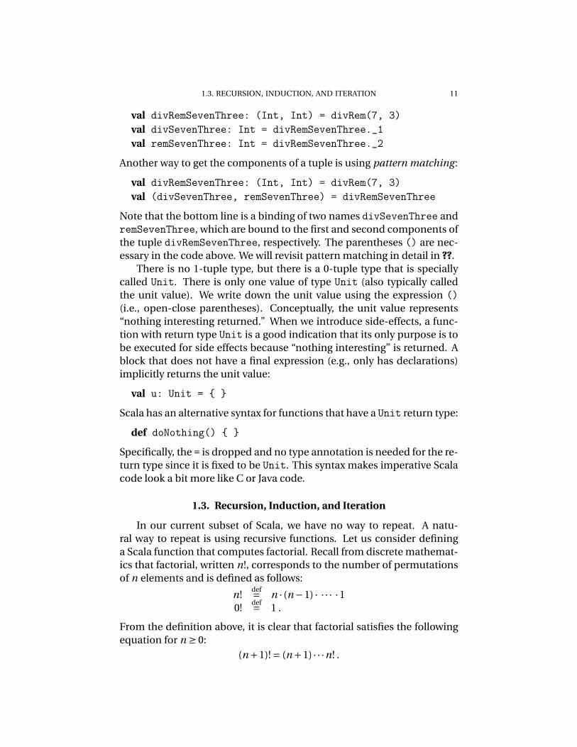
val divRemSevenThree: (Int, Int) = divRem(7, 3)val divSevenThree: Int = divRemSevenThree._1val remSevenThree: Int = divRemSevenThree._2
Another way to get the components of a tuple is using pattern matching:
val divRemSevenThree: (Int, Int) = divRem(7, 3)val (divSevenThree, remSevenThree) = divRemSevenThree
Note that the bottom line is a binding of two names divSevenThree andremSevenThree, which are bound to the first and second components ofthe tuple divRemSevenThree, respectively. The parentheses () are nec-essary in the code above. We will revisit pattern matching in detail in ??.
There is no 1-tuple type, but there is a 0-tuple type that is speciallycalled Unit. There is only one value of type Unit (also typically calledthe unit value). We write down the unit value using the expression ()(i.e., open-close parentheses). Conceptually, the unit value represents“nothing interesting returned.” When we introduce side-effects, a func-tion with return type Unit is a good indication that its only purpose is tobe executed for side effects because “nothing interesting” is returned. Ablock that does not have a final expression (e.g., only has declarations)implicitly returns the unit value:
val u: Unit = { }
Scala has an alternative syntax for functions that have a Unit return type:
def doNothing() { }
Specifically, the = is dropped and no type annotation is needed for the re-turn type since it is fixed to be Unit. This syntax makes imperative Scalacode look a bit more like C or Java code.
1.3. Recursion, Induction, and Iteration
In our current subset of Scala, we have no way to repeat. A natu-ral way to repeat is using recursive functions. Let us consider defininga Scala function that computes factorial. Recall from discrete mathemat-ics that factorial, written n!, corresponds to the number of permutationsof n elements and is defined as follows:
n!def= n · (n −1) · · · · ·1
0!def= 1 .
From the definition above, it is clear that factorial satisfies the followingequation for n ≥ 0:
(n +1)! = (n +1) · · ·n! .

12 1. INTRODUCTION AND PRELIMINARIES
Based on this equation, we can define a Scala function to compute facto-rial as follows:
LISTING 1.2. Factorial: A Basic Implementationdef factorial(n: Int): Int =
if (n == 0) 1 else factorial(n - 1) * n
Let us write out some steps of evaluating factorial(3):
factorial(3)−→ if (3 == 0) 1 else factorial(3 - 1) * 3−→∗ factorial(2) * 3−→∗ factorial(1) * 2 * 3−→∗ factorial(0) * 1 * 2 * 3−→∗ 1 * 1 * 2 * 3−→∗ 6
where the sequence above is shorthand for expressing that each succes-sive pair of expressions is related by the evaluation relation written be-tween them.
1.3.1. Induction: Reasoning about Recursive Programs. Inductionis important proof technique for reasoning about recursively-defined ob-jects that you might recall from a discrete mathematics course. Here, weconsider basic proofs of properties of recursive Scala functions.
The simplest form of induction is what we call mathematical induc-tion, that is, induction over natural numbers. Intuitively, to prove a prop-erty P over all natural numbers (i.e., ∀n ∈N.P (n)), we consider two cases:(a) we prove the property holds for 0 (i.e., P (0)), which is called the basecase; and (b) we prove that the property holds for n+1 assuming it holdsfor an n ≥ 0 (i.e., ∀n ∈N.(P (n) =⇒ P (n+1))), which is called the inductivecase.
As an example, let us prove that our Scala function factorial com-putes the mathematical definition of factorial n!. To state this propertyprecisely, we need a way to relate mathematical numbers with Scala val-ues. To do so, we use the notation xny to mean the Scala integer valuecorresponding to the mathematical number n.
THEOREM 1.1. For all integers n such that n ≥ 0,
factorial(xny) −→∗ xn!y .
PROOF. By mathematical induction on n.
BASE CASE (n = 0). Note that x0y = 0. Taking a few steps of evalua-tion, we have that
factorial(0) −→∗ 1 .

1.3. RECURSION, INDUCTION, AND ITERATION 13
Then, the Scala value 1 can also be written as x0!y because mathemati-cally 0! = 1.
INDUCTIVE CASE (n = n′+1 for some n′ ≥ 0). The induction hypoth-esis is as follows:
factorial(xn′y) −→∗ xn′!y .
Let us evaluate factorial(xny) a few steps, and we have the follow-ing:
factorial(xny) −→∗ factorial(xn −1y) * xny
because we know that n 6= 0. Applying the induction hypothesis, we havethat
xny * factorial(xn −1y) −→∗ xn′!y * xnynoting that n′ = n −1. By further evaluation, we have that
xn′!y * xny −→ xn′! ·ny .
Note that n′! ·n = n ·n′! = n · (n −1)! = n!, which completes this case. �
In the above, we are actually using an abstract notion of evaluationwhere Scala integer values are unbounded. In implementation, Scala in-tegers are in fact 32-bit signed two’s complement integers that we haveignored in our evaluation relation. It is often convenient to use abstractmodels of evaluation to essentially separate concerns. Here, we use anabstract model of evaluation to ignore overflow.
1.3.2. Pattern Matching. There is another style of writing recursivefunctions using pattern matching that looks somewhat closer to structureof an inductive proof. For example, we can write an implementation offactorial equivalent to Listing 1.2 as follows:
LISTING 1.3. Factorial: With Pattern Matchingdef factorial(n: Int): Int = n match {
case 0 => 1case _ => factorial(n - 1) * n
}
The match expression has the following form:
e match {case pattern1 => e1
. . .case patternn => en
}
14 1. INTRODUCTION AND PRELIMINARIES
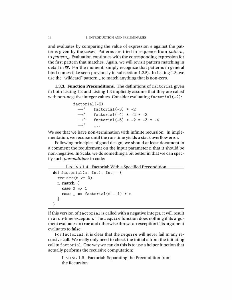
and evaluates by comparing the value of expression e against the pat-terns given by the cases. Patterns are tried in sequence from pattern1to patternn . Evaluation continues with the corresponding expression forthe first pattern that matches. Again, we will revisit pattern matching indetail in ??. For the moment, simply recognize that patterns in generalbind names (like seen previously in subsection 1.2.5). In Listing 1.3, weuse the “wildcard” pattern _ to match anything that is non-zero.
1.3.3. Function Preconditions. The definitions of factorial givenin both Listing 1.2 and Listing 1.3 implicitly assume that they are calledwith non-negative integer values. Consider evaluating factorial(-2):
factorial(-2)−→∗ factorial(-3) * -2−→∗ factorial(-4) * -2 * -3−→∗ factorial(-5) * -2 * -3 * -4−→∗ . . . .
We see that we have non-termination with infinite recursion. In imple-mentation, we recurse until the run-time yields a stack overflow error.
Following principles of good design, we should at least document ina comment the requirement on the input parameter n that it should benon-negative. In Scala, we do something a bit better in that we can spec-ify such preconditions in code:
LISTING 1.4. Factorial: With a Specified Preconditiondef factorial(n: Int): Int = {
require(n >= 0)n match {
case 0 => 1case _ => factorial(n - 1) * n
}}
If this version of factorial is called with a negative integer, it will resultin a run-time exception. The require function does nothing if its argu-ment evaluates to true and otherwise throws an exception if its argumentevaluates to false.
For factorial, it is clear that the require will never fail in any re-cursive call. We really only need to check the initial n from the initiatingcall to factorial. One way we can do this is to use a helper function thatactually performs the recursive computation:
LISTING 1.5. Factorial: Separating the Precondition fromthe Recursion

1.3. RECURSION, INDUCTION, AND ITERATION 15
def factorial(n: Int): Int = {require(n >= 0)def factorialRecurse(n: Int): Int = n match {
case 0 => 1case _ => factorialRecurse(n - 1) * n
}factorialRecurse(n)
}
Here, the factorialRecurse function is local to the factorial func-tion. The factorialRecurse does not do any checking on its argument,but the require check in factorialwill ensure that factorialRecursealways terminates.
1.3.4. Iteration: Tail Recursion with an Accumulator. Examining theevaluation of the various versions of factorial in this section, we ob-serve that they all behave similarly: (1) the recursion builds up an expres-sion consisting of a sequence of multiplication * operations, and then (2)the multiplication operations are evaluated to yield the result. In a typicalrun-time system, step (1) grows the call stack of activation records withrecursive calls recording pending evaluation (i.e., the * operation), andeach individual * operation in step (2) is executed while unwinding thecall stack on return. Our abstract notation for evaluation does not repre-sent a call stack implicitly, but we can see the corresponding behavior inthe growing “pending” expression.
Not all recursive functions require a call stack of activation records. Inparticular, when there’s nothing left to do on return, there is no “pendingcomputation” to record. This kind of recursive function is called tail re-cursive. A tail recursive version of the factorial function is given below inListing 1.6.
LISTING 1.6. Tail Recursive Factorial: Using an Accumulatordef factorial(n: Int): Int = {
require(n >= 0)def factorialIter(n: Int, acc: Int): Int = n match {
case 0 => acccase _ => factorialIter(n - 1, acc * n)
}factorialIter(n, 1)
}

16 1. INTRODUCTION AND PRELIMINARIES
Let us write out some steps of evaluating factorial(3) for this ver-sion:
factorial(3)−→ factorialIter(3, 1)−→∗ factorialIter(2, 1 * 3)−→ factorialIter(2, 3)−→∗ factorialIter(1, 3 * 2)−→ factorialIter(1, 6)−→∗ factorialIter(0, 6 * 1)−→ factorialIter(0, 6)−→∗ 6
Observe that the acc variable serves to accumulate the result. Whenwe reach the base case (i.e., 0), then we simply return the accumulatorvariable acc. Notice that there is no expression gets built up during thecourse of the recursion. When the last call to factorialIter returns,we have the final result. It is an important optimization for compilers torecognize tail recursion and avoid building a call stack unnecessarily.
A tail recursive function corresponds closely to a loop (e.g., a whileloop in language like Java) but does not require mutation. For example,consider the following version of factorial in Java using a while loopand variable assignment:
int factorial(int n) {int acc = 1;while (n > 0) {
acc = acc * n;n = n - 1;
}return acc;
}
Conceptually, each iteration of the while loop corresponds to a call offactorialIter. The value of acc and n in each iteration of the whileloop correspond to the values bound to acc and n on each recursive callto factorialIter.
1.4. LAB 1 17
1.4. Lab 1
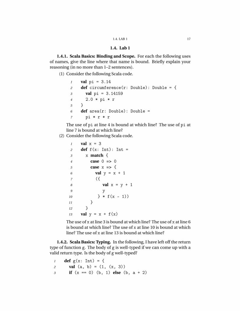
1.4.1. Scala Basics: Binding and Scope. For each the following usesof names, give the line where that name is bound. Briefly explain yourreasoning (in no more than 1–2 sentences).
(1) Consider the following Scala code.
1 val pi = 3.142 def circumference(r: Double): Double = {3 val pi = 3.141594 2.0 * pi * r5 }6 def area(r: Double): Double =7 pi * r * r
The use of pi at line 4 is bound at which line? The use of pi atline 7 is bound at which line?
(2) Consider the following Scala code.
1 val x = 32 def f(x: Int): Int =3 x match {4 case 0 => 05 case x => {6 val y = x + 17 ({8 val x = y + 19 y
10 } * f(x - 1))11 }12 }13 val y = x + f(x)
The use of x at line 3 is bound at which line? The use of x at line 6is bound at which line? The use of x at line 10 is bound at whichline? The use of x at line 13 is bound at which line?
1.4.2. Scala Basics: Typing. In the following, I have left off the returntype of function g. The body of g is well-typed if we can come up with avalid return type. Is the body of g well-typed?
1 def g(x: Int) = {2 val (a, b) = (1, (x, 3))3 if (x == 0) (b, 1) else (b, a + 2)

18 1. INTRODUCTION AND PRELIMINARIES
4 }
If so, give the return type of g and explain how you determined this type.For this explanation, first, give the types for the names a and b. Then,explain the body expression using the following format:
e : τ becausee1 : τ1 because
. . .e2 : τ2 because
. . .
where e1 and e2 are subexpressions of e. Stop when you reach values (ornames).
As an example of the suggested format, consider the plus function:
def plus(x: Int, y: Int) = x + y
Yes, the body expression of plus is well-typed with type Int.
x + y : Int becausex : Inty : Int
1.4.3. Run-Time Library. Most languages come with a standard li-brary with support for things like data structures, mathematical oper-ators, string processing, etc. Standard library functions may be imple-mented in the object language (perhaps for portability) or the meta lan-guage (perhaps for implementation efficiency).
For this question, we will implement some library functions in Scala,our meta language, that we can imagine will be part of the run-time forour object language interpreter. In actuality, the main purpose of thisexercise is to warm-up with Scala.
(1) Write a function abs
def abs(n: Double): Double
that returns the absolute value of n. This a function that takesa value of type Double and returns a value of type Double. Thisfunction corresponds to the JavaScript library function Math.abs.
Instructor Solution: 1 line.(2) Write a function xor
def xor(a: Boolean, b: Boolean): Boolean
that returns the exclusive-or of a and b. The exclusive-or returnstrue if and only if exactly one of a or b is true. For practice, donot use the Boolean operators. Instead, only use the if-else ex-pression and the Boolean literals (i.e., true or false).

1.4. LAB 1 19
Instructor Solution: 4 lines (including 1 line for a closingbrace).
1.4.4. Run-Time Library: Recursion.
(1) Write a recursive function repeat
def repeat(s: String, n: Int): String
where repeat(s, n) returns a string with n copies of s concate-nated together. For example, repeat("a",3) returns "aaa". Thisfunction corresponds to the function goog.string.repeat in theGoogle Closure library.
Instructor Solution: 4 lines (including 1 line for a closingbrace).
(2) In this exercise, we will implement the square root function—Math.sqrt in the JavaScript standard library. To do so, we willuse Newton’s method (also known as Newton-Raphson).
Recall from Calculus that a root of a differentiable functioncan be iteratively approximated by following tangent lines. Moreprecisely, let f be a differentiable function, and let x0 be an ini-tial guess for a root of f . Then, Newton’s method specifies a se-quence of approximations x0, x1, . . . with the following recursiveequation:7
xn+1 = xn − f (xn)
f ′(xn).
The square root of a real number c for c > 0, writtenp
c, is apositive x such that x2 = c. Thus, to compute the square root ofa number c, we want to find the positive root of the function:
f (x) = x2 − c .
Thus, the following recursive equation defines a sequence of ap-proximations for
pc:
xn+1 = xn − x2n − c
2xn.
(a) First, implement a function sqrtStep
def sqrtStep(c: Double, xn: Double): Double
that takes one step of approximation in computingp
c (i.e., com-putes xn+1 from xn).Instructor Solution: 1 line.
(b) Next, implement a function sqrtN
7The following link is a refresher video on this algorithm: http://www.youtube.com/watch?v=1uN8cBGVpfs, January 2012

20 1. INTRODUCTION AND PRELIMINARIES
def sqrtN(c: Double, x0: Double, n: Int): Double
that computes the nth approximation xn from an initial guessx0. You will want to call sqrtStep implemented in the previouspart.Challenge yourself to implement this function using recursionand no mutable variables (i.e., vars)—you will want to use a re-cursive helper function. It is also quite informative to compareyour recursive solution with one using a while loop.Instructor Solution: 7 lines (including 2 lines for closing bracesand 1 line for a require).
(c) Now, implement a function sqrtErr
def sqrtErr(c: Double, x0: Double,epsilon: Double): Double
that is very similar to sqrtN but instead computes approxima-tions xn until the approximation error is within ε (epsilon), thatis,
|x2n − c| < ε .
You can use your absolute value function abs implemented in aprevious part. A wrapper function sqrt is given in the templatethat simply calls sqrtErr with a choice of x0 and epsilon.Again, challenge yourself to implement this function using re-cursion and compare your recursive solution to one with a whileloop.Instructor Solution: 5 lines (including 1 line for a closing braceand 1 line for a require).
1.4.5. Data Structures Review: Binary Search Trees. In this ques-tion, we will review implementing operations on binary search trees fromData Structures. Balanced binary search trees are common in standardlibraries to implement collections, such as sets or maps. For example,the Google Closure library for JavaScript has goog.structs.AvlTree. Forsimplicity, we will not worry about balancing in this question.
Trees are important structures in developing interpreters, so this ques-tion is also critical practice in implementing tree manipulations.
A binary search tree is a binary tree that satisfies an ordering invari-ant. Let n be any node in a binary search tree whose data value is d , leftchild is l , and right child is r . The ordering invariant is that all of the datavalues in the subtree rooted at l must be < d , and all of the data values inthe subtree rooted at r must be ≥ d .

1.4. LAB 1 21
We will represent a binary trees containing integer data using the fol-lowing Scala case classes and case objects:
sealed abstract class SearchTreecase object Empty extends SearchTreecase class Node(l: SearchTree, d: Int, r: SearchTree) extends SearchTree
A SearchTree is either Empty or a Node with left child l, data value d,and right child r.
For this question, we will implement the following four functions.
(1) The function repOk
def repOk(t: SearchTree): Boolean
checks that an instance of SearchTree is valid binary search tree.In other words, it checks using a traversal of the tree the orderinginvariant. This function is useful for testing your implementa-tion. A skeleton of this function has been provided for you in thetemplate.
Instructor Solution: 7 lines (including 2 lines for closing braces).(2) The function insert
def insert(t: SearchTree, n: Int): SearchTree
inserts an integer into the binary search tree. Observe that thereturn type of insert is a SearchTree. This choice suggests afunctional style where we construct and return a new output treethat is the input tree t with the additional integer n as opposedto destructively updating the input tree.
Instructor Solution: 4 lines (including 1 line for a closingbrace).
(3) The function deleteMin
def deleteMin(t: SearchTree): (SearchTree, Int)
deletes the smallest data element in the search tree (i.e., the left-most node). It returns both the updated tree and the data valueof the deleted node. This function is intended as a helper func-tion for the delete function. Most of this function is provided inthe template.
Instructor Solution: 9 lines (including 2 lines for closing bracesand 1 line for a require).
(4) The function delete
def delete(t: SearchTree, n: Int): SearchTree
22 1. INTRODUCTION AND PRELIMINARIES
removes the first node with data value equal to n. This functionis trickier than insert because what should be done dependson whether the node to be deleted has children or not. We ad-vise that you take advantage of pattern matching to organize thecases.
Instructor Solution: 10 lines (including 2 lines for closingbraces).
1.4.6. JavaScripty Interpreter: Numbers. JavaScript is a complex lan-guage and thus difficult to build an interpreter for it all at once. In thiscourse, we will make some simplifications. We consider subsets of Java-Script and incrementally examine more and more complex subsets dur-ing the course of the semester. For clarity, let us call the language that weimplement in this course JAVASCRIPTY.
For the moment, let us define JAVASCRIPTY to be a proper subset of Ja-vaScript. That is, we may choose to omit complex behavior in JavaScript,but we want any programs that we admit in JAVASCRIPTY to behave in thesame way as in JavaScript.
In actuality, there is not one language called JavaScript but a set ofclosely related languages that may have slightly different semantics. Indeciding how a JAVASCRIPTY program should behave, we will consult areference implementation that we fix to be Google’s V8 JavaScript Engine.We will run V8 via Node.js, and thus, we will often need to write little testJavaScript programs and run it through Node.js to see how the test shouldbehave.
In this lab, we consider an arithmetic sub-language of JavaScript (i.e.,an extremely basic calculator). The first thing we have to consider is howto represent a JAVASCRIPTY program as data in Scala, that is, we need to beable to represent a program in our object/source language JAVASCRIPTY
as data in our meta/implementation language Scala.To a JAVASCRIPTY programmer, a JAVASCRIPTY program is a text file—
a string of characters. Such a representation is quite cumbersome towork with as a language implementer. Instead, language implementa-tions typically work with trees called abstract syntax trees (ASTs). Whatstrings are considered JAVASCRIPTY programs is called the concrete syntaxof JAVASCRIPTY, while the trees (or terms) that are JAVASCRIPTY programsis called the abstract syntax of JAVASCRIPTY. The process of convertinga program in concrete syntax (i.e., as a string) to a program in abstractsyntax (i.e., as a tree) is called parsing.
For this lab, a parser is provided for you that reads in a JAVASCRIPTY
program-as-a-string and converts into an abstract syntax tree. We willrepresent abstract syntax trees in Scala using case classes and case objects.

1.4. LAB 1 23
sealed abstract class Exprcase class N(n: Double) extends Expr
N(n) ncase class Unary(uop: Uop, e1: Expr) extends Expr
Unary(uop, e1) uope1
case class Binary(bop: Bop, e1: Expr, e2: Expr) extends ExprBinary(bop, e1, e2) e1 bop e2
sealed abstract class Uopcase object Neg extends Uop
Neg −
sealed abstract class Bopcase object Plus extends Bop
Plus +case object Minus extends Bop
Minus −case object Times extends Bop
Times ∗case object Div extends Bop
Div /
FIGURE 1.1. Representing in Scala the abstract syntax ofJAVASCRIPTY. After each case class or case object, we showthe correspondence between the representation and theconcrete syntax.
The correspondence between the concrete syntax and the abstract syntaxrepresentation is shown in Figure 1.1.
(1)
INTERPRETER 1.1. Implement the eval function
def eval(e: Expr): Double
that evaluates a JAVASCRIPTY expression e to the Scala double-precision floating point number corresponding to the value ofe.
Consider a JAVASCRIPTY program e; imagine e stands for the concretesyntax or text of the JAVASCRIPTY program. This text is parsed into aJAVASCRIPTY AST e, that is, a Scala value of type Expr. Then, the resultof eval is a Scala number of type Double and should match the interpre-tation of e as a JavaScript expression. These distinctions can be subtle
24 1. INTRODUCTION AND PRELIMINARIES
but learning to distinguish between them will go a long way in makingsense of programming languages.
At this point, you have implemented your first language interpreter!

CHAPTER 2
Approaching a Programming Language
We have studied subsets of Scala up to this point mostly by example.At some point, we may wonder (1) what are all the Scala programs thatwe can write, and (2) what do they mean? The answer to question (1) isgiven by a definition of Scala’s syntax, while the answer to question (2) isgiven by a definition of Scala’s semantics.
As a language designer, it is critical to us that we define unambigu-ously the syntax and semantics so that everyone understands our intent.Language users need to know what they can write and how the programsthey write will execute as alluded to in the previous paragraph. Languageimplementers need to know what are the possible input strings and whatthey mean in order to produce semantically-equivalent output code.
2.1. Syntax: Grammars and Scoping
Stated informally, the syntax of a language is concerned with the formof programs, that is, the strings that we consider programs. The seman-tics of a language is concerned with the meaning of programs, that is,how programs evaluate. Because there an unbounded number of pos-sible programs in a language, we need tools to speak more abstractlyabout them. Here, we focus on describing the syntax of programminglanguages. We will consider defining the semantics of programming lan-guages in section 3.1.
The concrete syntax of a programming language is concerned withhow to write down expressions, statements, and programs as strings. Con-crete syntax is the primary interface between the language user and thelanguage implementation. Thus, the design of concrete syntax focuseson improving readability and perhaps writability for software develop-ers. There are significant sociological considerations, such as appealingto tradition (e.g., using curly braces { . . . } to denote blocks of statements).A large part of concrete syntax design is a human-computer interactionproblem, which is outside of what we can consider in this course.
The abstract syntax of a programming language is the representationof programs used by language implementations and thus an importantmental model for language implementers and language users. We will
25

26 2. APPROACHING A PROGRAMMING LANGUAGE
draw out precisely the distinction between concrete and abstract syntaxin this section.
2.1.1. Context-Free Languages and Context-Free Grammars. A lan-guage L is a set of strings composed of characters drawn from some al-phabet Σ (i.e., L ⊆ Σ∗). A string in a language is sometimes called a sen-tence.
The standard way to describe the concrete syntax of a language isusing context-free grammars. A context-free grammar is a way to de-scribe a class of languages called context-free languages. A context-freegrammar defines a language inductively and consists of terminals, non-terminals, and productions. Terminals and non-terminals are genericallycalled symbols. The terminals of a grammar correspond to the alphabetof the language being defined and are the basic building blocks. Non-terminals are defined via productions and conceptually recognize a se-quence of symbols belonging to a sublanguage. A production has theform N ::= α where N is a non-terminal from the set of non-terminalsN and α is a sequence of symbols (i.e., α ∈ (Σ∪N )∗). A set of of pro-ductions with the same non-terminal, such as N ::= α1, . . . , N ::= αn , isusually written with one instance of the non-terminal and the right-handsides separated by |, such as N ::= α1 | · · · | αn . Such a set of productionscan be read informally as, “N is generated by either α1, . . ., or αn .” Forany non-terminal N , we can talk about the language or syntactic categorydefined by that non-terminal.
As an example, let us consider defining a language of integers as fol-lows:
integers i ::= −n | nnumbers n ::= d | d ndigits d ::= 0 | 1 | 2 | 3 | 4 | 5 | 6 | 7 | 8 | 9
with the alphabet Σdef= {0,1,2,3,4,5,6,7,8,9,−}. We identify the overall
language by the start non-terminal (also called the start symbol). By con-vention, we typically consider the non-terminal listed first as the startnon-terminal. Here, we have strings like 1, 2, 42, 100, and −7 in ourlanguage of integers. Note that strings like 012 and −0 are also in thislanguage.
2.1.1.1. Derivation of a Sentence in a Grammar. Formally, a string isin the language described by a grammar if and only if we can give a deriva-tion for it from the start symbol. We say a sequence of symbols β is de-rived from another sequence of symbols α, written as
α =⇒ β ,

2.1. SYNTAX: GRAMMARS AND SCOPING 27
when β is obtained by replacing a non-terminal N in α with the right-hand side of a production of N . We can a give witness that a string s be-longs to a language by showing derivation steps from the start symbol tothe string s. For example, we show that 012 is in the language of integersdefined above:
i =⇒ n=⇒ d n=⇒ 0 n=⇒ 0 d n=⇒ 01 n=⇒ 01 d=⇒ 012 .
In the above, we have shown a leftmost derivation, that is, one where wealways choose to expand the leftmost non-terminal. We can similarly de-fine a rightmost derivation. Note that there are typically several deriva-tions that witness a string belonging the language described by a gram-mar.
We can now state precisely the language described by a grammar. LetL (G) be the language described by grammar G over the alphabet Σ, startsymbol S, and derivation relation =⇒. We define the relation α=⇒∗ β asholding if and only if β can be derived from α with the one-step deriva-tion relation =⇒ in zero or more steps (i.e., =⇒∗ is the reflexive-transitiveclosure of =⇒). Then, L (G) is defined as follows:
L (G)def= {
s∣∣ s ∈Σ∗ and S =⇒∗ s
}.
2.1.2. Lexical and Syntactic. In language implementations, we of-ten want to separate the simple grouping of characters from the iden-tification of structure. For example, when we read the string 23 + 45,we would normally see three pieces: the number twenty-three, the plusoperator, and the number forty-five, rather than the literal sequence ofcharacters ‘2’, ‘3’, ‘ ’, ‘+’, ‘ ’, ‘4’, and ‘5’.
Thus, it is common to specify the lexical structure of a language sep-arately from the syntactic structure. The lexical structure is this simplegrouping of characters, which is often specified using regular expressions.A lexer transforms a sequence of literal characters into a sequence of lex-emes classified into tokens. For example, a lexer might transform thestring "23+45" into the following sequence:
num("23"),+,num("45")
consisting of three tokens: a num token with lexeme "23", a plus tokenwith lexeme "+", and a num token with lexeme "45". Since there is only

28 2. APPROACHING A PROGRAMMING LANGUAGE
one possible lexeme for the plus token, we abuse notation slightly andname the token by the lexeme.
A parser then recognizes strings of tokens, typically specified usingcontext-free grammars. For example, we might define a language of ex-pressions with numbers and the plus operator:
expr ::= num | expr + expr .
Note that num is a terminal in this grammar.There is an analogy to parsing sentences in natural languages. Group-
ing letters into words in a sentence corresponds essentially to lexing, whileclassifying words into grammatical elements (e.g., nouns, verbs, nounphrases, verb phrases) corresponds to parsing.
2.1.3. Ambiguous Grammars. Consider the following arithmetic ex-pression:
100/10/5 .
Should it be read as (100/10)/5 or 100/(10/5)? The former equals 2, whilethe latter equals 50. In mathematics, we adopt conventions that, for ex-ample, choosing the former over the latter.
Now consider a language implementation that is given the followinginput:
100/10/5 .
Which reading should it take? In particular, consider the grammar
e ::= n | e / e
where n is the terminal for numbers. We can diagram the two ways ofreading the string 100/10/5 as shown in Figures 2.1c and 2.1d where wewrite the lexemes for the n tokens in parentheses for clarity. These di-agrams are called parse trees, and they are another way to demonstratethat a string is the language described by a grammar. In a parse tree,a parent node corresponds to a non-terminal where its children corre-spond to the sequence of symbols in a production of that non-terminal.Parse trees capture syntactic structure and distinguishes between the twoways of “reading” 100/10/5. We call the grammar given above ambigu-ous because we can witness a string that is “read” in two ways by givingtwo parse trees for it.
As an aside, in this way, a parse tree can be viewed as “recognizing”a string by a grammar in a “bottom-up manner.” In contrast, derivationsintuitively capture generating strings described a grammar in a “top-downmanner.”
Can we rewrite the above grammar to make it unambiguous? That is,can we rewrite the above grammar such that the set of strings accepted

2.1. SYNTAX: GRAMMARS AND SCOPING 29
e ::= n | e / e
(A) Grammar.
100/10/5(B)String.
e
e
e
n(100)
/ e
n(10)
/ e
n(5)
(C) Parse tree.
e
e
n(100)
/ e
e
n(10)
/ e
n(5)
(D) Parse tree.
FIGURE 2.1. An ambiguous grammar is exhibited by twoparse trees for a string in the language described by thegrammar.
Ambiguous Unambiguous
Left Recursive Right Recursive
e ::= n | e / e e ::= n | e / n e ::= n | n / e
FIGURE 2.2. Rewriting a grammar to eliminate ambiguitywith respect to associativity.
by the grammar is the same but is also unambiguous. Yes, we can rewritethe above grammar in two ways to eliminate ambiguity as shown in Fig-ure 2.2. One grammar is left recursive, that is, the production e ::= e / n isrecursive only on the left of the binary operator token /. Analogously, wecan write a right recursive grammar that accepts the same strings. Intu-itively, these grammars enforce a particular linearization of the possibleparse trees: either to the left or to the right as shown in Figure 2.3. As aterminological shorthand, we say that a binary operator is left associativeto mean that expression trees involving that operator are linearized to theleft, as in Figure 2.3c). Analogously, a binary operator is right associativemeans expression trees involving that operator are linearized to the right,as in Figure 2.3e.
A related syntactic issue appears when we consider multiple opera-tors, such as the ambiguous grammar in Figure 2.4. For example, thestring
10−10/10

30 2. APPROACHING A PROGRAMMING LANGUAGE
100/10/5(A)String.
e ::= n | e / n
(B) Left-recursive.
e
e
e
n(100)
/ n(10)
/ n(5)
(C) Parse tree.
e ::= n | n / e
(D) Right-recursive.
e
n(100) / e
n(10) / e
n(5)
(E) Parse tree.
FIGURE 2.3. Grammars that enforce a particular associativity.
Ambiguous Unambiguous
e ::= n | e / e | e − ee ::= f | e − ff ::= n | f / n
FIGURE 2.4. Rewriting a grammar to eliminate ambiguityand enforce a particular associativity (left for both opera-tors) and precedence (/ higher than −).
has two parse trees corresponding to the following two readings:
(10−10)/10 or 10−(10/10) .
We may want to enforce that the / operator “binds tighter,” that is, hashigher precedence than the − operator, which corresponds to the read-ing on the right. To enforce the desired precedence, we can refactor theambiguous grammar into the unambiguous one shown in Figure 2.4. Welayer the grammar by introducing a new non-terminal f that describesexpressions with only / operator. The non-terminal f is left recursive,so we enforce that / is left associative. The start non-terminal e can beeither an f or an expression with a − operator. Intuitively from a top-down, derivation perspective, once e =⇒ f , then there is no way to derivea − operator. Thus, in any parse tree for a string that includes both − and/ operators, the − operators must be “higher” in the tree. Note that higher

2.1. SYNTAX: GRAMMARS AND SCOPING 31
precedence means “binding tighter” or “lower in the parse tree” and sim-ilarly for lower precedence.
An important observation is that ambiguity is a syntactic concern:which tree do we get when we parse a string? This concern is differentthan and distinct with respect to what do the / or the − operators mean(e.g., perhaps division and subtraction), that is, the semantics of our ex-pression language or to what value does an expression evaluate. The is-sue is the same if we consider a language with a pair operators that havea less ingrained meaning, such as @ and #.
If we know semantics of the language, then we can sometimes probeto determine associativity or precedence. For example, let us suppose weare interested in seeing what is relative precedence of the / and − oper-ators in Scala. Knowing that / means division and − means subtraction,then observing the value of the expression 10−10/10 tells us the relativeprecedence of these two operators. Specifically, if the value is 9, then / hashigher precedence, but if the value is 0, then − has higher precedence.
2.1.4. Abstract Syntax. Consider again the grammar of expressionsinvolving the / and − operators in Figure 2.4, with subscripts to makeexplicit the instances of the symbols:
e ::= n | e1 / e2 | e1 − e2
To represent expressions e in Scala, we declare the following types andcase classes:
sealed abstract class Exprcase class N(n: Int) extends Exprcase class Divide(e1: Expr, e2: Expr) extends Exprcase class Minus(e1: Expr, e2: Expr) extends Expr
We define a new type Expr (i.e., an abstract class). Each case class is aconstructor for an expression e of type Expr corresponding to one of theproductions defining the non-terminal e.
If we rewrite the above grammar to use these constructor names ineach production, we get the following:
e ∈ Expr ::= N(n) | Divide(e1, e2) | Minus(e1, e2) .
An example sentence in this language is
Minus(N(10), Divide(N(10), N(10))) ,
which corresponds to the following sentence in the first grammar:
10−10/10 .
Observe that a different sentence in the second grammar
Divide(Minus(N(10), N(10)), N(10))

32 2. APPROACHING A PROGRAMMING LANGUAGE
also corresponds to 10−10/10. While the first grammar is ambiguous,the second one is unambiguous.
In a language implementation, we do not want to be constantly wor-rying about the “grouping” or parsing of a string (i.e., resolving ambigu-ity), so we prefer to work with terms in this second grammar. We call thissecond grammar, abstract syntax, as the tree structure is evident. Eachinstance of case class is a node in an n-ary tree and each argument of anon-terminal type to a constructor is a sub-tree. For example, the termMinus(N(10), Divide(N(10), N(10))) can be read visually as the following:
Minus
N(10) Divide
N(10) N(10)
And thus the first phase of language tool is the parser that converts theconcrete syntax of strings into the abstract syntax of terms.
Because the concrete syntax is more concise visually and human fri-endly, it is standard practice to give (ambiguous) grammars like the firstgrammar above and treat them as the corresponding abstract syntax spec-ification given in the second grammar. In other words, we give a grammarthat define the strings of a language and leave it as an implementationdetail of the parser to convert strings to the appropriate terms or abstractsyntax trees. We even often draw abstract syntax trees using concrete syn-tax notation, such as
−
10 /
10 10 .
2.2. Structural Induction
As we have seen, a convenient way to represent programs for manipu-lation by algorithms are as abstract syntax trees. In Scala, case classes areparticularly useful for representing trees. Operations over trees are natu-rally given by recursive traversals, and pattern matching makes it easierto implement such recursive walks over abstract syntax trees.
In section 1.3, we saw that there is a tight connection between recur-sive programs and inductive reasoning. Learning to think inductively en-ables us to more easily implement correct, complex recursive traversalsthat are requisite for implementing any language tools.

2.2. STRUCTURAL INDUCTION 33
Here, we introduce the concept of structural induction that enablesus to reason not just over natural numbers but over any inductive type.Like in subsection 1.3.1, we focus on proving properties of recursive pro-grams really with the goal of learning to think inductively.
2.2.1. Structural Induction over Lists. Consider the definition of Scalalists (simplified):
sealed abstract class List[T]case object Nil extends List[Nothing]case class ::[T](head: T, tail: List[T]) extends List[T]
Let us consider the possibles values of type List[Int], for example. Here’swhat this set looks like schematically:
{ Nil,0 :: Nil, 1 :: Nil, −1 :: Nil, . . . ,0 :: 0 :: Nil, 1 :: 0 :: Nil, −1 :: 0 :: Nil, . . . ,0 :: 1 :: Nil, 1 :: 1 :: Nil, −1 :: 1 :: Nil, . . . }
This set is inductively defined and can be viewed as generated by apply-ing “rules” corresponding to Nil and ::. Thus, we have an induction prin-ciple for proving properties about List[T] values. Intuitively, to prove aproperty P over all List[T] values (i.e., ∀l : List[T].P (l )), we consider twocases: (a) we prove that the property holds for Nil, that is, P (Nil)—a basecase; and (b) we prove that the property holds for h::t assuming it holdsfor t (for any h : T and any t : List[T]), that is, ∀h : T, t : List[T].(P (t ) =⇒P (h :: t ))—an inductive case. Notice the similarity to mathematical in-duction described in subsection 1.3.1. In fact, mathematical induction issimply a special case of structural induction over natural numbers.
As an example, consider the definition of list append given in List-ing 2.1. Let us show that append terminates for any input. This propertyis extremely simple, but it illustrates the structure of such a proof.
LISTING 2.1. List Appenddef append[T](xl: List[T], yl: List[T]): List[T] =
xl match {case Nil => ylcase xh :: xt => xh :: append(xt, yl)
}
THEOREM 2.1 (Termination of append). For all values xl and yl of typeList[T],
append(xl, yl) −→∗ l
for some value l .
34 2. APPROACHING A PROGRAMMING LANGUAGE
PROOF. By structural induction on xl.
BASE CASE (xl = Nil). Taking a few steps of evaluation, we have that
append(xl, yl)= append(Nil, yl)
−→∗ yl (by the definition of append)
Note that yl is a value, so this case is complete.
INDUCTIVE CASE (xl = h::t for some values h : T and t : List[T]). Theinduction hypothesis is as follows:
append(t , yl) −→∗ tl for some value tl.
Let us evaluate append(xl, yl) a few steps, and we have the following:
append(xl, yl)= append(h::t , yl)
−→∗ h :: append(t , yl) (by the definition of append)
By the induction hypothesis (i.h.) on t , we have that
append(t , yl)−→∗ tl .
for some value tl. Thus, we have that
h :: append(t , yl)−→∗ h::tl
Note that h::tl is a value, so this case is complete.
�
There are a number of key things to observe about the above proof.First, we chose xl as the induction variable. We have two inductively de-fined values xl and yl over which we are universally quantifying, so wecould induct on either one. However, xl is the only choice that will allowus to complete this proof. Choosing the appropriate structure on whichto apply induction can get tricky in general and sometimes requires trial-and-error. However, for correctness of recursive functions, choosing thevalue on which the recursion is over is almost always a good choice. Inthis case, append in Listing 2.1 is defined recursively over its first argu-ment (i.e., xl).
Once the induction variable is chosen, the “proof template” is au-tomatic. There is a case for each way the value could be constructed(e.g., Nil and :: in the case of List[T] values). Any case that has a sub-component of the inductively-defined type is an inductive case (e.g., ::),while any case that does not is a base case (e.g., Nil). Furthermore, theinductive hypothesis is also automatic in each inductive case—the prop-erty being proven is assumed to hold for any sub-component of the in-ductively-defined type (e.g., the tail of the list). Once you get familiar
2.2. STRUCTURAL INDUCTION 35
enough with induction, it becomes acceptable to leave off stating the in-duction hypothesis, as it is understood. When applying the induction hy-pothesis, it is important to state to which sub-component the inductionhypothesis is being applied, as in some inductively-defined types therecan be multiple sub-components. In the above, for example, we statedthat the induction hypothesis was applied to the tail list t .
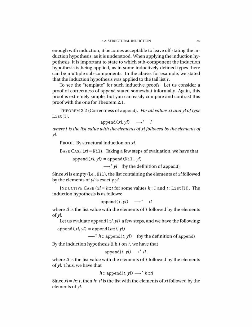
To see the “template” for such inductive proofs. Let us consider aproof of correctness of append stated somewhat informally. Again, thisproof is extremely simple, but you can easily compare and contrast thisproof with the one for Theorem 2.1.
THEOREM 2.2 (Correctness of append). For all values xl and yl of typeList[T],
append(xl, yl) −→∗ l
where l is the list value with the elements of xl followed by the elements ofyl.
PROOF. By structural induction on xl.
BASE CASE (xl = Nil). Taking a few steps of evaluation, we have that
append(xl, yl)= append(Nil, yl)
−→∗ yl (by the definition of append)
Since xl is empty (i.e., Nil), the list containing the elements of xl followedby the elements of yl is exactly yl.
INDUCTIVE CASE (xl = h::t for some values h : T and t : List[T]). Theinduction hypothesis is as follows:
append(t , yl) −→∗ tl
where tl is the list value with the elements of t followed by the elementsof yl.
Let us evaluate append(xl, yl) a few steps, and we have the following:
append(xl, yl)= append(h::t , yl)
−→∗ h :: append(t , yl) (by the definition of append)
By the induction hypothesis (i.h.) on t , we have that
append(t , yl)−→∗ tl .
where tl is the list value with the elements of t followed by the elementsof yl. Thus, we have that
h :: append(t , yl)−→∗ h::tl
Since xl = h::t , then h::tl is the list with the elements of xl followed by theelements of yl.
36 2. APPROACHING A PROGRAMMING LANGUAGE
�
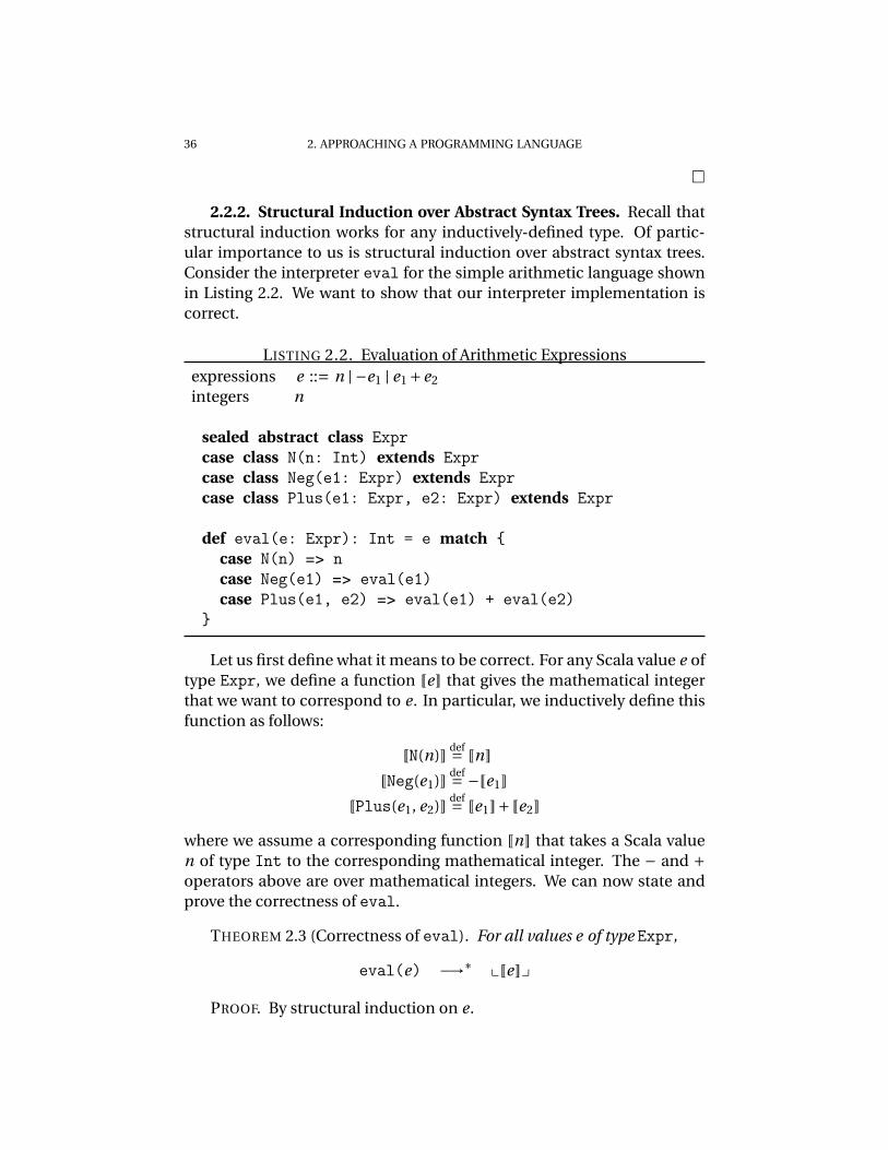
2.2.2. Structural Induction over Abstract Syntax Trees. Recall thatstructural induction works for any inductively-defined type. Of partic-ular importance to us is structural induction over abstract syntax trees.Consider the interpreter eval for the simple arithmetic language shownin Listing 2.2. We want to show that our interpreter implementation iscorrect.
LISTING 2.2. Evaluation of Arithmetic Expressionsexpressions e ::= n | −e1 | e1 +e2
integers n
sealed abstract class Exprcase class N(n: Int) extends Exprcase class Neg(e1: Expr) extends Exprcase class Plus(e1: Expr, e2: Expr) extends Expr
def eval(e: Expr): Int = e match {case N(n) => ncase Neg(e1) => eval(e1)case Plus(e1, e2) => eval(e1) + eval(e2)
}
Let us first define what it means to be correct. For any Scala value e oftype Expr, we define a function �e� that gives the mathematical integerthat we want to correspond to e. In particular, we inductively define thisfunction as follows:
�N(n)� def= �n��Neg(e1)� def= −�e1�
�Plus(e1, e2)� def= �e1�+�e2�where we assume a corresponding function �n� that takes a Scala valuen of type Int to the corresponding mathematical integer. The − and +operators above are over mathematical integers. We can now state andprove the correctness of eval.
THEOREM 2.3 (Correctness of eval). For all values e of type Expr,
eval(e) −→∗ x�e�y
PROOF. By structural induction on e.

2.2. STRUCTURAL INDUCTION 37
BASE CASE (e = N(n) for some value n : Int). Taking a few steps ofevaluation, we have that
eval(e)= eval(N(n))
−→∗ n (by the definition of eval)
Note that x�N(n)�y= x�n�y= n, so this case is complete.
INDUCTIVE CASE (e = Neg(e1) for some value e1 : Expr). Taking a fewsteps of evaluation, we have that
eval(e)= eval(Neg(e1))
−→∗ −eval(e1) (by the definition of eval)
By the i.h. on e1, we have that
eval(e1)−→∗ x�e1�y .
Thus, we have that
−eval(e1)−→∗ −x�e1�y−→∗ x−�e1�y (by the definition of − in Scala)
Note that x�Neg(e1)�y= x−�e1�y, so this case is complete.
INDUCTIVE CASE (e = Plus(e1, e2) for some values e1 : Expr and e2 : Expr).Taking a few steps of evaluation, we have that
eval(e)= eval(Plus(e1, e2))
−→∗ eval(e1)+eval(e1) (by the definition of eval)
By the i.h. on e1, we have that
eval(e1)−→∗ x�e1�y .
And by the i.h. on e2, we have that
eval(e2)−→∗ x�e2�y .
Thus, we have that
eval(e1)+eval(e1)−→∗ x�e1�y+x�e2�y−→∗ x�e1�+�e2�y (by the definition of + in Scala)
Note that x�Plus(e1, e2)�y= x�e1�+�e2�y, so this case is complete.
�
38 2. APPROACHING A PROGRAMMING LANGUAGE
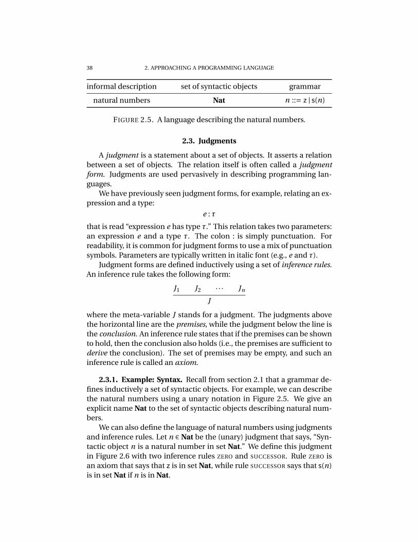
informal description set of syntactic objects grammar
natural numbers Nat n ::= z | s(n)
FIGURE 2.5. A language describing the natural numbers.
2.3. Judgments
A judgment is a statement about a set of objects. It asserts a relationbetween a set of objects. The relation itself is often called a judgmentform. Judgments are used pervasively in describing programming lan-guages.
We have previously seen judgment forms, for example, relating an ex-pression and a type:
e : τ
that is read “expression e has type τ.” This relation takes two parameters:an expression e and a type τ. The colon : is simply punctuation. Forreadability, it is common for judgment forms to use a mix of punctuationsymbols. Parameters are typically written in italic font (e.g., e and τ).
Judgment forms are defined inductively using a set of inference rules.An inference rule takes the following form:
J1 J2 · · · Jn
J
where the meta-variable J stands for a judgment. The judgments abovethe horizontal line are the premises, while the judgment below the line isthe conclusion. An inference rule states that if the premises can be shownto hold, then the conclusion also holds (i.e., the premises are sufficient toderive the conclusion). The set of premises may be empty, and such aninference rule is called an axiom.
2.3.1. Example: Syntax. Recall from section 2.1 that a grammar de-fines inductively a set of syntactic objects. For example, we can describethe natural numbers using a unary notation in Figure 2.5. We give anexplicit name Nat to the set of syntactic objects describing natural num-bers.
We can also define the language of natural numbers using judgmentsand inference rules. Let n ∈ Nat be the (unary) judgment that says, “Syn-tactic object n is a natural number in set Nat.” We define this judgmentin Figure 2.6 with two inference rules ZERO and SUCCESSOR. Rule ZERO isan axiom that says that z is in set Nat, while rule SUCCESSOR says that s(n)is in set Nat if n is in Nat.

2.3. JUDGMENTS 39
n ∈ NatZERO
z ∈ Nat
SUCCESSOR
n ∈ Nat.
s(n) ∈ Nat
FIGURE 2.6. Defining the language of natural numbers judgmentally.
n1 =Nat n2
ZERO-EQ
z=Nat z
SUCCESSOR-EQ
n1 =Nat n2
s(n1) =Nat s(n2)
FIGURE 2.7. Defining structural equality of natural numbers.
2.3.2. Derivations of Judgments. A set of inference rules defines ajudgment as the least relation closed under the rules. This statementmeans a judgment holds if and only if we can compose applications ofthe inference rules to demonstrate it. Such a demonstration is called aderivation. A derivation is a tree where each node in the tree is an appli-cation of an inference rule and whose children are derivations of the rule’spremises. The leaves of a derivation tree are applications of axioms.
For example, to demonstrate that the judgment s(s(z)) ∈ Nat holds, wegive the following the derivation:
z ∈ NatZERO
s(z) ∈ NatSUCCESSOR
s(s(z)) ∈ NatSUCCESSOR
.
We write the rule that is applied to the right of the horizontal line.
2.3.3. Structural Induction on Derivations. Judgments are induct-ively-defined relations. They yield an induction principle based on thestructure of derivations. In particular, to show a property P (J ) wheneverJ holds, it suffices to consider each rule from which J may be derived:
J1 J2 · · · Jn
J
and show P (J ) under the inductive hypotheses P (J1), P (J2), . . ., and P (Jn).
40 2. APPROACHING A PROGRAMMING LANGUAGE
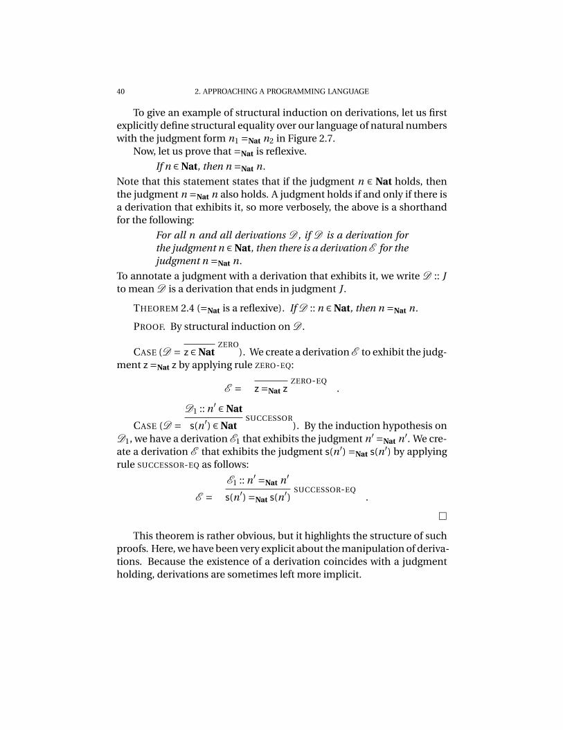
To give an example of structural induction on derivations, let us firstexplicitly define structural equality over our language of natural numberswith the judgment form n1 =Nat n2 in Figure 2.7.
Now, let us prove that =Nat is reflexive.
If n ∈ Nat, then n =Nat n.
Note that this statement states that if the judgment n ∈ Nat holds, thenthe judgment n =Nat n also holds. A judgment holds if and only if there isa derivation that exhibits it, so more verbosely, the above is a shorthandfor the following:
For all n and all derivations D , if D is a derivation forthe judgment n ∈ Nat, then there is a derivation E for thejudgment n =Nat n.
To annotate a judgment with a derivation that exhibits it, we write D :: Jto mean D is a derivation that ends in judgment J .
THEOREM 2.4 (=Nat is a reflexive). If D :: n ∈ Nat, then n =Nat n.
PROOF. By structural induction on D .
CASE (D = z ∈ NatZERO
). We create a derivation E to exhibit the judg-ment z=Nat z by applying rule ZERO-EQ:
E = z=Nat zZERO-EQ
.
CASE (D =D1 :: n′ ∈ Nat
s(n′) ∈ NatSUCCESSOR
). By the induction hypothesis onD1, we have a derivation E1 that exhibits the judgment n′ =Nat n′. We cre-ate a derivation E that exhibits the judgment s(n′) =Nat s(n′) by applyingrule SUCCESSOR-EQ as follows:
E =E1 :: n′ =Nat n′
s(n′) =Nat s(n′)SUCCESSOR-EQ
.
�
This theorem is rather obvious, but it highlights the structure of suchproofs. Here, we have been very explicit about the manipulation of deriva-tions. Because the existence of a derivation coincides with a judgmentholding, derivations are sometimes left more implicit.

CHAPTER 3
Language Design and Implementation
3.1. Operational Semantics
In section 2.1, we began the discussion of language specification andthe importance specifying languages clearly, crisply, and precisely. Gram-mars is the main tool by which the syntax of a language, that is, the pro-grams that we can write are specified. In this section, we introduce a toolfor defining the semantics of a language, that is, the meaning of programs.
There are several ways to think about the meaning of program. Onenatural way is to think about how program evaluate. An operational se-mantics is a way to describe how programs evaluate in terms of the lan-guage itself (rather than by compilation to a machine model). One way tosee an operational semantics is as describing an interpreter for the lan-guage of interest.
3.1.1. Syntax: JavaScripty. We consider a small subset of JavaScript,which we will affectionately call JAVASCRIPTY. The syntax of JAVASCRIPTY
is given in Figure 3.1. Recall that we interpret such a definition as theabstract syntax of JAVASCRIPTY using elements from its concrete syntax.That is, we write concrete syntax for readability but assume that we aregiven abstract syntax trees that resolve ambiguity in the grammar.
expressions e ::= x | n | b | undefined | uope1 | e1 bop e2
| e1 ? e2 : e3 | const x = e1; e2 | console.log(e1)values v ::= n | b | undefinedunary operators uop ::= - | !binary operators bop ::= , | + | - | * | / | < | <= | > | >=
| === | !== | && | ||variables xnumbers (doubles) nbooleans b ::= true | false
FIGURE 3.1. Syntax of JAVASCRIPTY
41
42 3. LANGUAGE DESIGN AND IMPLEMENTATION
Figure 3.1 describes JAVASCRIPTY using a number of syntactic cate-gories. The main syntactic category is expressions. We consider a pro-gram to be an expression. Expressions e consist of variables, value lit-erals, unary operator expressions, binary operator expressions, a condi-tional if-then-else expression, a variable binding expression, and a printexpression. Values v can be numbers (double-precision floating point),booleans, and a unique undefined value. This set of essentially arith-metic expressions is the usual core of any programming language. Func-tions are notably missing.
3.1.2. A Big-Step Operational Semantics. We might guess the seman-tics of particular expressions based on common conventions. For exam-ple, we probably guess that expression
e1 + e2
adds two numbers that result from evaluating e1 and e2. However, notethat this statement something about the semantics of e1 + e2, which hasyet to be specified.
One aspect that makes the JavaScript specification complex is the pres-ence of implicit conversions (e.g., boolean values may be implicitly con-verted to numeric values depending on the context in which values areused). For example,
true + 2
evaluates to 3. How can we describe how to implement a JAVASCRIPTY
interpreter for all programs?It is possible to specify the semantics of a programming language us-
ing natural language prose. However, just like with specifying syntax us-ing natural language prose, it is very easy to leave ambiguity in the de-scription. Furthermore, trying to minimize ambiguity can create veryverbose descriptions. The JavaScript specification, specifically ECMA-262 standard [], is actually rather precise specification based on naturallanguage prose, but the descriptions are quite verbose.
In this section, we introduce some mathematical notation that en-ables us to specify semantics with less ambiguity in a very compact form.Like any mathematical notation, its precise and compact nature makesit easier, for example, to spot errors or inconsistencies in specification.However, there will necessarily be a learning curve to reading the nota-tion.
We want to write out as unambiguously as possible how a programshould evaluate independent of an implementation (e.g., a compiler and

3.1. OPERATIONAL SEMANTICS 43
machine architecture). We use a method specification known as an oper-ational semantics. An operational semantics can be thought as describ-ing an interpreter for the language of interest with relations between syn-tactic objects. We have already used a notation for describing an evalua-tion relation:
e ⇓ v .
This notation is a judgment form stating informally, “Expression e eval-uates to value v .” Defining this judgment describes how to evaluate ex-pressions to values and thus corresponds closely to writing a recursiveinterpreter of the abstract syntax trees representing expressions.
We will use a slight richer judgment form with an additional parame-ter:
E ` e ⇓ v ,
which says informally, “In value environment E , expression e evaluatesto value v .” This relation has three parameters: E , e, and v . The otherparts of the judgment is simply punctuation that separates the parame-ters. The ` symbol is called the “turnstile” symbol.
A value environment E is a finite map from variables x to values v andcan be described by the following grammar:
E ::= · | E [ x 7→ v] .
We write · for the empty environment and E [ x 7→ v] as the environmentthat maps x to v but is otherwise the same as E (i.e., extends E with map-ping x to v). Additionally, we write E(x) for looking up the value of x inenvironment E . More precisely, we can define look up as follows:
E [ y 7→ v](x)def= v if y = x
E [ y 7→ v](x)def= E(x) otherwise
·(x) undefined .
The inference rules that define this evaluation judgment form is givenin Figure 3.2. Let us first consider the two axioms:
EVALVAR
E ` x ⇓ E(x)
EVALVAL
E ` v ⇓ v.
The EVALVAR rule says that a variable use x evaluates to the value to whichit is bound in the environment E . Or operationally, to evaluate a variableuse x, look up the value corresponding to x in the environment E . For anexpression that is already a value v , it evaluates to itself as stated by theEVALVAL rule.
Now, back to the original example in this section, we are trying tospecify how the expression
e1 + e2

44 3. LANGUAGE DESIGN AND IMPLEMENTATION
evaluates. Thinking operationally, we want to say something like: evalu-ate e1 to a number, evaluate e2 to a number, and then return the numberthat is the addition of those numbers. Consider the following inferencerule:
E ` e1 ⇓ n1 E ` e2 ⇓ n2 n′ = n1+n2
E ` e1 +e2 ⇓ n′
Reading top-down, this rule says if we know that in environment E , ex-pression e1 evaluates to a number n1 and e2 evaluates to n2, then expres-sion e1 + e2 evaluates to n′ in environment E where n′ is the additionof the n1 and n2. Note that the + in the premise is “plus” in the metalanguage (i.e., the implementation language) in contrast to the + in theconclusion that is the syntactic symbol + in the object language (i.e., thesource language). Here, we have highlighted the meta-language “plus”for clarity, but often, the reader is asked to determine this distinctionbased on context. To be completely explicit, we could use an alternativenotation for the abstract syntax:
E ` e1 ⇓ n1 E ` e2 ⇓ n2 n′ = n1+n2
E ` Binary(Plus, e1, e2) ⇓ n′
This rule defines a semantics that does not fully match JavaScript be-cause it requires e1 and e2 in e1 + e2 to evaluate to number values (i.e.,n1 and n2). JavaScript permits other types of values and then performs aconversion before performing the addition. We can express this seman-tics using the following inference rule:
E ` e1 ⇓ v1 E ` e2 ⇓ v2 n′ = toNumber(v1)+ toNumber(v2)
E ` e1 +e2 ⇓ n′
Reading top-down, it says if we know that in environment E , expressione1 evaluates to v1 and e2 evaluates to v2, then expression e1 + e2 evaluatesto n′ in environment E where n′ is the addition of the toNumber conver-sions of v1 and v2. We define the toNumber conversion in Figure 3.3. Thisrule specifies the semantics that we want, though it is not the only way todo so.
Any evaluation rule can also be read bottom-up, which matches moreclosely to an implementation. For example, the above rule says, “To eval-uate e1 + e2 in environment E , evaluate e1 in environment E to get valuev1, evaluate e2 in environment E to get value v2, convert v1 and v2 tonumbers, and return the addition of those two numbers.”
In Figure 3.2, we lump all of the arithmetic operators +, −, ∗, and /together in the same rule: EVALARITH. We use one notational shortcut

3.1. OPERATIONAL SEMANTICS 45
E ` e ⇓ v
EVALVAR
E ` x ⇓ E(x)
EVALVAL
E ` v ⇓ v
EVALNEGE ` e1 ⇓ v1 n′ =− toNumber(v1)
E `−e1 ⇓ n′
EVALNOTE ` e1 ⇓ v1 b′ =¬ toBoolean(v1)
E ` !e1 ⇓ b′
EVALSEQE ` e1 ⇓ v1 E ` e2 ⇓ v2
E ` e1 , e2 ⇓ v2
EVALARITHE ` e1 ⇓ v1 E ` e2 ⇓ v2 n′ = toNumber(v1) bop toNumber(v2) bop ∈ {+,−,∗,/}
E ` e1 bop e2 ⇓ n′
EVALINEQUALITYE ` e1 ⇓ v1 E ` e2 ⇓ v2 b′ = toNumber(v1) bop toNumber(v2) bop ∈ {<,<=,>,>=}
E ` e1 bop e2 ⇓ b′
EVALEQUALITYE ` e1 ⇓ v1 E ` e2 ⇓ v2 b′ = (v1 bop v2) bop ∈ {===, ! ==}
E ` e1 bop e2 ⇓ b′
EVALANDTRUEE ` e1 ⇓ v1 true = toBoolean(v1) E ` e2 ⇓ v2
E ` e1 && e2 ⇓ v2
EVALANDFALSEE ` e1 ⇓ v1 false = toBoolean(v1)
E ` e1 && e2 ⇓ v1
EVALORTRUEE ` e1 ⇓ v1 true = toBoolean(v1)
E ` e1 || e2 ⇓ v1
EVALORFALSEE ` e1 ⇓ v1 false = toBoolean(v1) E ` e2 ⇓ v2
E ` e1 || e2 ⇓ v2
EVALPRINTE ` e1 ⇓ v1 v1 printed
E ` console.log(e1) ⇓ undefined
EVALIFTRUEE ` e1 ⇓ v1 true = toBoolean(v1) E ` e2 ⇓ v2
E ` e1 ? e2 : e3 ⇓ v2
EVALIFFALSEE ` e1 ⇓ v1 false = toBoolean(v1) E ` e3 ⇓ v3
E ` e1 ? e2 : e3 ⇓ v3
EVALCONSTE ` e1 ⇓ v1 E [ x 7→ v1] ` e2 ⇓ v2
E ` const x = e1; e2 ⇓ v2
FIGURE 3.2. Big-step operational semantics of JAVASCRIPTY.
by treating the bop as the corresponding meta-language operator in thepremise.
It is informative to study the complete set of inference rules and thinkabout how the rules correspond to implementing an interpreter. TheEVALCONST rule is particularly interesting because we see explicitly that
const x = e1; e2
the scope of variable x is the expression e2 because e2 is evaluated in anextended environment with a binding for x.

46 3. LANGUAGE DESIGN AND IMPLEMENTATION
toNumber(n)def= n
toNumber(true)def= 1
toNumber(false)def= 0
toNumber(undefined)def= NaN
toBoolean(n)def= false if n = 0 or n =NaN
toBoolean(n)def= true otherwise
toBoolean(b)def= b
toBoolean(undefined)def= false
FIGURE 3.3. JAVASCRIPTY conversion functions.
3.2. Small-Step Operational Semantics
3.2.1. Evaluation Order. In subsection 3.1.2, we have carefully spec-ified several aspects of how the expression
e1 + e2
should be evaluated. In essence, it adds two integers that result fromevaluating e1 and e2. However, there is still at least one more semanticquestion that we have not specified, “Is e1 evaluated first and then e2 orvice versa, or are they evaluated concurrently?”
Why does this question matter? Consider the expression:
(3.2.1.1) (jsy.print(1), 1) + (jsy.print(2), 2) .
The , operator is a sequencing operator. In particular, e1 , e2 first evalu-ates e1 to a value and then evaluates e2 to value; the value of the wholeexpression is the value of e2, while the value of e1 is simply thrown away.Furthermore, console.log(e1) evaluates its argument to a value and thenprints to the screen a representation of that value. If the left operand ofa + is evaluated first before the right operand, then the above expression(3.2.1.1) prints 1 and then 2. If the operands of + are evaluated in the op-posite order, then 2 is printed first followed by 1. Note that the final valueis 3 regardless of the evaluation order.
The evaluation order matters because the console.log(e1) expressionhas a side effect. It prints to the screen. As alluded to in section 1.2, an ex-pression free of side effects (i.e., is pure) has the advantage that the eval-uation order cannot be observed (i.e., does not matter from the program-mer’s perspective). Having this property is also known as being referen-tially transparent, that is, taking an expression and replacing any of itssubexpressions by the subexpression’s value cannot be observed as eval-uating any differently than evaluating the expression itself. In JAVASCRIPTY,our only side-effecting expression is console.log(e1). If we remove the

3.2. SMALL-STEP OPERATIONAL SEMANTICS 47
prints from the above expression (3.2.1.1), then the evaluation order can-not be observed.
3.2.2. A Small-Step Operational Semantics of JAVASCRIPTY. The big-step operational semantics given in subsection 3.1.2 does give us a nicespecification for implementing an interpreter, but it does leave some se-mantic choices like evaluation order implicit. Intuitively, it specifies whatthe value of an expression should be (if it exists) but not precisely thesteps to get to the value.
We have already used a notation for describing a one-step evaluationrelation:
e −→ e ′ .
This notation is a judgment form stating informally, “Expression e cantake one step of evaluation to expression e ′.” Defining this judgment al-lows us to more precisely state how to take one step of evaluation, thatis, how to make a single reduction step. Once we know how to reduceexpressions, we can evaluate an expression e by repeatedly applying re-duction until reaching a value. Thus, such a definition describes an op-erational semantics and intuitively an interpreter for expressions e. Thisstyle of operational semantics where we specify reduction steps is calleda small-step operational semantics.
In contrast to subsection 3.1.2, we will not extend this judgment formwith value environments. Instead, we define the one-step reduction rela-tion on closed expressions, that is, expressions without any free variables.If we require the “top-level” program to be a closed expression, then wecan ensure reduction only sees closed expressions by intuitively “apply-ing the environment” eagerly via substitution. That is, variable uses arereplaced by the values to which they are bound before reduction gets tothem. As an example, we will define reduction so that the following judg-ment holds:
const x = 1; x + x −→ 1 + 1 .
This choice to use substitution instead of explicit environments is or-thogonal to specifying the semantics using small-step or big-step (i.e.,one could use subsitution with big-step or environments with small-step).Explicit environments just get a bit more unwieldy here.
First, we need to describe what action does an operation perform. Forexample, we want to say that the + operator adds to numbers, which wesay with the following rule:
DOPLUS
n′ = toNumber(v1)+ toNumber(v2)
v1 + v2 −→ n′

48 3. LANGUAGE DESIGN AND IMPLEMENTATION
This rules says the expression v1 + v2 reduces in one step to an integervalue n′ that is the addition of the toNumber conversion of values v1 andv2. We use the meta-variables v1, v2, and n′ to express constraints thatparticular positions in the expressions must be values or numeric values.Note that the + in the conclusion is the syntactic + operator, while the +in the premise expresses mathematical addition of two numbers. As wediscussed in subsection 3.1.2, this symbol clash is rather unfortunate, butcontext usually allows us to determine which + is which. We sometimescall this kind of rule that performs an operation a local reduction rule. Wewill prefix all rules for this kind of rule with DO (and so will sometimescall them DO rules).
Second, we need to describe how we find the next operation to per-form. These rules will capture issues like evaluation order described in-formally in subsection 3.2.1. To specify that e1 + e2 should be evaluatedleft-to-right, we use the following two rules:
SEARCHPLUS1
e1 −→ e ′1
e1 + e2 −→ e ′1 + e2
SEARCHPLUS2
e2 −→ e ′2
v1 + e2 −→ v1 + e ′2
The SEARCHPLUS1 rule states for an arbitrary expression of the form e1 +e2, if e1 steps to e ′
1, then the whole expression steps to e ′1 + e2. We can
view this rule as saying that we should look for an operation to performsomewhere in e1. The rest of the expression • + e2 is a context that getscarried over untouched. The SEARCHPLUS2 rule is similar except that itapplies only if the left expression is a value (i.e., v1 + e2). Together, theserules capture precisely a left-to-right evaluation order for an expressionof the form e1 + e2 because (1) if e1 is not a value, then only SEARCHPLUS1
could possibly apply, and (2) if e1 is a value, then only SEARCHPLUS2 couldpossibly apply. We sometimes call this kind of rule that finds the nextoperation to perform a global reduction rule (or a SEARCH rule). The sub-expression that is the next operation to perform is called the redex.
Considering these three rules, there is at most one rule that appliesthat specifies the “next” step. If our set of inference rules defining reduc-tion has this property, then we say that our reduction system is determin-istic. In other words, there is always at most one “next” step. Determin-ism is a property that we could prove about certain reduction systems,which we can state formally as follows:
PROPERTY 3.1 (Determinism). If e −→ e ′ and e −→ e ′′, then e ′ = e ′′.
In general, such a proof would proceed by structural induction on thederivation of the reduction step (i.e., e −→ e ′). We do not yet such proofshere in detail (cf., subsection 2.3.3).

3.2. SMALL-STEP OPERATIONAL SEMANTICS 49
e −→ e ′
DONEGn′ =− toNumber(v)
−v −→ n′
DONOTb′ =¬ toBoolean(v)
! v −→ b′DOSEQ
v1 , e2 −→ e2
DOARITHn′ = toNumber(v1) bop toNumber(v2) bop ∈ {+,−,∗,/}
v1 bop v2 −→ n′
DOINEQUALITYb′ = toNumber(v1) bop toNumber(v2) bop ∈ {<,<=,>,>=}
v1 bop v2 −→ b′
DOEQUALITYb′ = (v1 bop v2) bop ∈ {===, ! ==}
v1 bop v2 −→ b′
DOANDTRUEtrue = toBoolean(v1)
v1 && e2 −→ e2
DOANDFALSEfalse = toBoolean(v1)
v1 && e2 −→ false
DOORTRUEtrue = toBoolean(v1)
v1 || e2 −→ true
DOORFALSEfalse = toBoolean(v1)
v1 || e2 −→ e2
DOPRINTv1 printed
console.log(v1) −→ undefined
DOIFTRUEtrue = toBoolean(v1)
v1 ? e2 : e3 −→ e2
DOIFFALSEfalse = toBoolean(v1)
v1 ? e2 : e3 −→ e3
DOCONST
const x = v1; e2 −→ e2[v1/x]
SEARCHUNARYe1 −→ e′1
uope1 −→ uope′1
SEARCHBINARY1e1 −→ e′1
e1 bop e2 −→ e′1 bop e2
SEARCHBINARY2e2 −→ e′2
v1 bop e2 −→ v1 bop e′2
SEARCHPRINTe1 −→ e′1
console.log(e1) −→ console.log(e′1)
SEARCHIFe1 −→ e′1
e1 ? e2 : e3 −→ e′1 ? e2 : e3
SEARCHCONSTe1 −→ e′1
const x = e1; e2 −→ const x = e′1; e2
FIGURE 3.4. Small-step operational semantics of JAVASCRIPTY.
In Figure 3.4, we give all of the inference rules that define the one-step evaluation relation e −→ e ′ for JAVASCRIPTY. The DONEG states thatthe unary operator − is integer negation, while DONOT states that ! isboolean negation. Observe that to “do” the operation, we require that thesub-expression under the unary operators − or !, respectively, is a value.Contrast these rules to EVALNEG and EVALNOT in Figure 3.2. If the sub-expression under the unary operator is not a value, then instead the ruleSEARCHUNARY applies telling us to look for something to reduce insidethis sub-expression. The DOSEQ rules states that the ‘,’ operator is used

50 3. LANGUAGE DESIGN AND IMPLEMENTATION
to indicate sequencing: for e1 , e2, first e1 is evaluated to a value, thenthat value is ignored, and we continue by evaluating e2. The DOARITH,DOINEQUALITY, and DOEQUALITY specify how the arithmetic, inequality,and equality operators behave, respectively. The DOARITH includes thecase for + that we separated out in our discussion above.
We say that a short-circuit evaluation of expression is one where avalue is produced before evaluating all subexpressions to values. Thenext four rules DOANDTRUE, DOANDFALSE, DOORTRUE, and DOORFALSE saythat the boolean expressions e1 && e2 and e1 || e2 may short-circuit. Inparticular, the rule
DOANDFALSE
false = toBoolean(v1)
v1 && e2 −→ false
says that v1 && e2 where v1 converts to false evaluates to false withoutever evaluating e2. The analogous rule for || is
DOORTRUE
true = toBoolean(v1)
v1 || e2 −→ true
The DOPRINT rule
DOPRINT
v1 printed
console.log(v1) −→ undefined
is somewhat informal. In particular, since printing is outside of our model,the“v1 printed” in the premise of the rule is not any required conditionbut should be viewed as comment for when this rule is applied. What isstated is the result of a print is the value undefined.
For e1 ? e2 : e3, the rules DOIFTRUE and DOIFFALSE specify with whichexpression to continue evaluation in the expected way depending on whatBoolean value to which the guard converts.
The DOCONST rule for the variable binding expression const x = e1; e2
DOCONST
const x = v1; e2 −→ e2[v1/x]
is a bit more interesting. The expression-to-be-bound should already bea value v1. We then proceed with e2 with the value v1 replacing the vari-able x. In general, the notation e1[e2/x] is read as capture-avoiding sub-stitution of expression e2 for variable x in e1. We describe substitution inmore detail below in subsubsection 3.2.2.1.

3.2. SMALL-STEP OPERATIONAL SEMANTICS 51
The remaining rules in Figure 3.4 describe how to find the next op-eration to perform (i.e., the global reduction rules). They specify that allexpressions are evaluated left-to-right.
3.2.2.1. Substitution. The term capture-avoiding subsitution meansthat we get the expression that is like e1, but we have replaced all in-stances of variable x with e2 while carefully repecting static scoping (cf.,subsection 1.2.4). There are two throny issues that arise.
Shadowing: The substitution
(const a = 1; a + b)︸ ︷︷ ︸e1
[ 2︸︷︷︸e2
/ a︸︷︷︸x
]
should yield (const a = 1; a + b). That is, only free instancesof a in e1 should be replaced.
Free Variable Capture: The substutition
(const a = 1; a + b)︸ ︷︷ ︸e1
[(a + 2)︸ ︷︷ ︸e2
/ b︸︷︷︸x
]
should yield something like (const c = 1; c + (a + 2)). Inparticular, the following result is wrong:
(const a = 1; a + (a + 2))
because the free variable a in e2 gets “captured” by the constbinding of a.
In both cases, the issues could be resolved by renaming all bound vari-ables in e1 so that there are no name conflicts with free variables in e2 orx. In other words, it is clear what to do if e1 were instead
const c = 1; c + b
in which case textual substitution would suffice.The observation is that renaming bound variables should preserve
the meaning of the expression, that is, the following two expressions aresomehow equivalent:
(const a = 1; a) ≡α (const b = 1; b)
For historical reasons, this equivalence is known α-equivalence, and theprocess of renaming bound variables is called α-renaming. This obser-vation also leads to coming up with an abstract syntax representation sothat the above two expressions are represented with the same object. Asan aside, one way to do this is to use variables in the meta language torepresent variables in the object langauge. This idea is known as higher-order abstract syntax.
In DOCONST, our situation is slight more restricted than the generalcase discussed above. In particular, the substitution is of the form e[v/x]
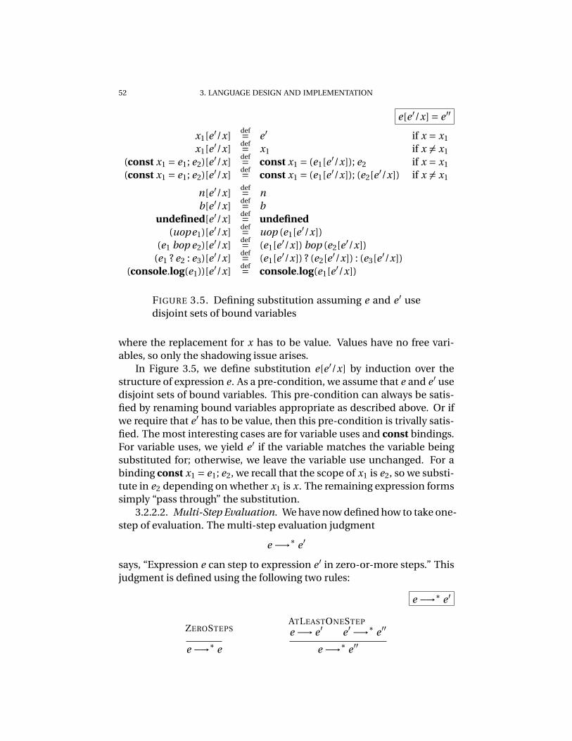
52 3. LANGUAGE DESIGN AND IMPLEMENTATION
e[e ′/x] = e ′′
x1[e ′/x]def= e ′ if x = x1
x1[e ′/x]def= x1 if x 6= x1
(const x1 = e1; e2)[e ′/x]def= const x1 = (e1[e ′/x]); e2 if x = x1
(const x1 = e1; e2)[e ′/x]def= const x1 = (e1[e ′/x]); (e2[e ′/x]) if x 6= x1
n[e ′/x]def= n
b[e ′/x]def= b
undefined[e ′/x]def= undefined
(uope1)[e ′/x]def= uop (e1[e ′/x])
(e1 bop e2)[e ′/x]def= (e1[e ′/x]) bop (e2[e ′/x])
(e1 ? e2 : e3)[e ′/x]def= (e1[e ′/x]) ? (e2[e ′/x]) : (e3[e ′/x])
(console.log(e1))[e ′/x]def= console.log(e1[e ′/x])
FIGURE 3.5. Defining substitution assuming e and e ′ usedisjoint sets of bound variables
where the replacement for x has to be value. Values have no free vari-ables, so only the shadowing issue arises.
In Figure 3.5, we define substitution e[e ′/x] by induction over thestructure of expression e. As a pre-condition, we assume that e and e ′ usedisjoint sets of bound variables. This pre-condition can always be satis-fied by renaming bound variables appropriate as described above. Or ifwe require that e ′ has to be value, then this pre-condition is trivally satis-fied. The most interesting cases are for variable uses and const bindings.For variable uses, we yield e ′ if the variable matches the variable beingsubstituted for; otherwise, we leave the variable use unchanged. For abinding const x1 = e1; e2, we recall that the scope of x1 is e2, so we substi-tute in e2 depending on whether x1 is x. The remaining expression formssimply “pass through” the substitution.
3.2.2.2. Multi-Step Evaluation. We have now defined how to take one-step of evaluation. The multi-step evaluation judgment
e −→∗ e ′
says, “Expression e can step to expression e ′ in zero-or-more steps.” Thisjudgment is defined using the following two rules:
e −→∗ e ′
ZEROSTEPS
e −→∗ e
ATLEASTONESTEP
e −→ e ′ e ′ −→∗ e ′′
e −→∗ e ′′

3.2. SMALL-STEP OPERATIONAL SEMANTICS 53
In other words, −→∗ is the reflexive-transitive closure of −→.A property that we want is that our big-step semantics and our small-
step semantics are “the same.” We can state this property formally asfollows.
PROPERTY 3.2 (Big-Step and Small-Step Equivalence). · ` e ⇓ v if andonly if e −→∗ v.

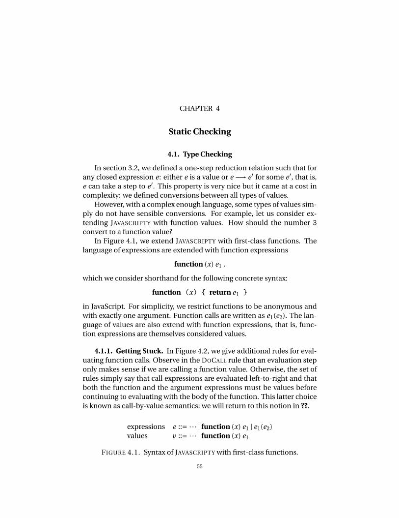
CHAPTER 4
Static Checking
4.1. Type Checking
In section 3.2, we defined a one-step reduction relation such that forany closed expression e: either e is a value or e −→ e ′ for some e ′, that is,e can take a step to e ′. This property is very nice but it came at a cost incomplexity: we defined conversions between all types of values.
However, with a complex enough language, some types of values sim-ply do not have sensible conversions. For example, let us consider ex-tending JAVASCRIPTY with function values. How should the number 3
convert to a function value?In Figure 4.1, we extend JAVASCRIPTY with first-class functions. The
language of expressions are extended with function expressions
function (x) e1 ,
which we consider shorthand for the following concrete syntax:
function (x) { return e1 }
in JavaScript. For simplicity, we restrict functions to be anonymous andwith exactly one argument. Function calls are written as e1(e2). The lan-guage of values are also extend with function expressions, that is, func-tion expressions are themselves considered values.
4.1.1. Getting Stuck. In Figure 4.2, we give additional rules for eval-uating function calls. Observe in the DOCALL rule that an evaluation steponly makes sense if we are calling a function value. Otherwise, the set ofrules simply say that call expressions are evaluated left-to-right and thatboth the function and the argument expressions must be values beforecontinuing to evaluating with the body of the function. This latter choiceis known as call-by-value semantics; we will return to this notion in ??.
expressions e ::= ·· · | function (x) e1 | e1(e2)values v ::= ·· · | function (x) e1
FIGURE 4.1. Syntax of JAVASCRIPTY with first-class functions.
55

56 4. STATIC CHECKING
DOCALL
(function (x) e1)(v2) −→ e1[v2/x]
SEARCHCALL1
e1 −→ e ′1
e1(e2) −→ e ′1(e2)
SEARCHCALL2
e2 −→ e ′2(
function (x) e1)(e2) −→ (
function (x) e1)(e ′
2)
FIGURE 4.2. Small-step operational semantics ofJAVASCRIPTY with first-class functions (extends Figure 3.4).
TYPEERRORCALL
v1 6= function p(x) e1
v1(e2) −→ typeerror
PROPAGATECALL1
typeerror(e2) −→ typeerror
PROPAGATECALL2
v1(typeerror) −→ typeerror
Other PROPAGATE rules for other expressionforms not shown.
FIGURE 4.3. Extending the small-step semantics ofJAVASCRIPTY from Figure 4.2 with dynamic type errors.
Note that these rules do not say anything about how to evaluate anill-typed expression, such as
3(4) .
Intuitively, evaluating this expression should result in an error. We do notstate this error explicitly. Rather, we see that this an expression that is (1)not value and (2) can make no further progress (i.e., there’s no rule thatspecifies a next expression). We call such an expression a stuck expres-sion, which captures the idea that it is erroneous in some way.
4.1.2. Dynamic Typing. Another formalization and implementationchoice would be to make such ill-typed expressions step to an error to-ken. For example, we add to the expression language a token typeerrorrepresenting a dynamic type error:
expressions e ::= ·· · | typeerrorAn ill-typed function call now steps to typeerror with rule TYPEERRORCALL.We also need to extend rules for evaluating other all other expression

4.1. TYPE CHECKING 57
expressions e ::= ·· · | function (x : τ) e1
values v ::= ·· · | function (x : τ) e1
types τ ::= number | bool | Undefined | (x : τ) ⇒ τ′
type environments Γ ::= · | Γ[ x 7→ τ]
FIGURE 4.4. Restricting JAVASCRIPTY with static typing.
forms that propagate the typeerror token if one is encountered in search-ing for a redex. We show PROPAGATECALL1 and PROPAGATECALL2, whichare two such rules, that correspond to SEARCHCALL1 and SEARCHCALL2, re-spectively.
With this instrumentation, we distinguish a dynamic type error forany other reason for getting stuck. For example, an expression with freevariables, such as
x .
Recall that our one-step evaluation relation is intended for closed expres-sions, so we might view this an internal error of the interpreter imple-mentation rather than an error in the input JAVASCRIPTY program.
4.1.3. Static Typing. In subsection 4.1.1, we saw how “bad” expres-sions, such as,
3(4)
are erroneous according to our operational semantics in that they “getstuck.” This expression gets stuck because a call expression e1(e2) onlyapplicable to function values. We say that such an expression 3(4) is ill-typed or not well-typed.
A type is a classification of values that characterize the valid opera-tions for these values. A type system consists of a language of types anda typing judgment that defines when an expression has a particular type.When we say that an expression e has a type τ, we mean that if e evaluatesto a value, then that value should be of type τ. In this way, a type systempredicts some property about how an expression evaluates at run-time.
In Figure 4.4, we show a language of types τ for JAVASCRIPTY that in-cludes base types for numbers n : number, Booleans b : bool, and theundefined value undefined : Undefined, as well as a constructed type forfunction values. A function type (x : τ) ⇒ τ′ classifies function valueswhose return value has type τ′ assuming its called with an argument oftype τ. Our expression language e has modified slightly to add type an-notations to function parameters.
A typing judgment form is defined by a set of typing rules that is thefirst step towards defining a type checking algorithm. A type error is an

58 4. STATIC CHECKING
expression that violates the prescribed typing rules (i.e., may produce avalue outside the set of values that it is supposed to have). We define atyping judgment form inductively on the syntactic structure of programobjects (e.g., expressions).
Recall from our earlier discussion on binding (subsection 1.2.3) thatthe type of an expression with free variable depends on an environment.In other words, consider the expression
x + 1 .
Is this expression well-typed? It depends. If in the environment, x isstated to type Int, then it is well-typed; otherwise, it is not. We see thatthe type of an expression e depends on a type environment Γ that givesthe types of the free variables of e. Thus, our typing judgment form is asfollows:
Γ` e : τ
that says informally, “In typing environment Γ, expression e has typeτ.” Observe how similar this judgment form is to our big-step evalua-tion judgment form from subsection 3.1.2. This observation is a bit morethan a coincidence. A standard type checker works by inferring the typeof an expression by recursively inferring the type of each sub-expression.A big-step interpreter computes the value of an expression by recursivelycomputing the value of each sub-expression. In essence, we can view atype checker as an abstract evaluator over a type abstraction of concretevalues.
In Figure 4.5, we define typing of JAVASCRIPTY. The first four rulesTYPENUMBER, TYPEBOOL, TYPEUNDEFINED, and TYPEFUNCTION describe thetypes of values. The types of the primitive values n, b, and undefined areas expected. The TYPEFUNCTION is more interesting:
TYPEFUNCTION
Γ[ x 7→ τ] ` e : τ′
Γ` function (x : τ) e : (x : τ) ⇒ τ′
A function value has a function type (x : τ) ⇒ τ′ (also sometimes calledsimply an “arrow” type) whose parameter type is τ and return type is τ′.The return type τ′ is obtained by inferring the type of the body expressione under the extended environment Γ[ x 7→ τ].
Examining the typing rules for the unary operators, we see that wehave decided to restrict the input programs beyond those that get stuckwith the small-step semantics defined in Figure 4.2:
TYPENEG
Γ` e1 : number
Γ`−e1 : number
TYPENOT
Γ` e1 : bool
Γ` !e1 : bool

4.1. TYPE CHECKING 59
Γ` e : τ
TYPENUMBER
Γ` n : number
TYPEBOOL
Γ` b : bool
TYPEUNDEFINED
Γ` undefined : Undefined
TYPEFUNCTIONΓ[ x 7→ τ] ` e : τ′
Γ` function (x : τ) e : (x : τ) ⇒ τ′TYPEVAR
Γ` x : Γ(x)
TYPENEGΓ` e1 : number
Γ`−e1 : number
TYPENOTΓ` e1 : bool
Γ` !e1 : bool
TYPESEQ
Γ` e1 : τ1 Γ` e2 : τ2
Γ` e1 , e2 : τ2
TYPEARITHΓ` e1 : number Γ` e2 : number bop ∈ {+,−,∗,/}
Γ` e1 bop e2 : number
TYPEINEQUALITY
Γ` e1 : number Γ` e2 : number bop ∈ {<,<=,>,>=}
Γ` e1 bop e2 : bool
TYPEEQUALITY
Γ` e1 : τ Γ` e2 : τ τ has no function types bop ∈ {===, ! ==}
Γ` e1 bop e2 : bool
TYPEANDORΓ` e1 : bool Γ` e2 : bool bop ∈ {&&, ||}
Γ` e1 bop e2 : bool
TYPEPRINTΓ` e1 : τ1
Γ` console.log(e1) : Undefined
TYPEIFΓ` e1 : bool Γ` e2 : τ Γ` e3 : τ
Γ` e1 ? e2 : e3 : τ
TYPECONSTΓ` e1 : τ1 Γ[ x 7→ τ1] ` e2 : τ2
Γ` const x = e1; e2 : τ2
TYPECALLΓ` e1 : (x : τ) ⇒ τ′ Γ` e2 : τ
Γ` e1(e2) : τ′
FIGURE 4.5. Typing of JAVASCRIPTY.
For example, with rule TYPENEG, we say that −e1 is well-typed if e1 hastype number. Furthermore, this rule is the only rule for −e1, so we areonly permitting unary negation − of numbers. Similarly, we are only per-mit not ! applied to booleans. Thus, only code that does not need conver-sions is well typed. Therefore, we can simplify our interpreter to get rid

60 4. STATIC CHECKING
of conversions if only allow executing well-typed programs. We continuewith this design choice in this set of rules.
In the sequencing rule TYPESEQ
TYPESEQ
Γ` e1 : τ1 Γ` e2 : τ2
Γ` e1 , e2 : τ2,
the type of the sequencing expression is τ2. The type of e1 is checked butthen dropped—all we care about is that e1 is well typed. Even thoughwe are dropping the type, the expression still needs to be type checkedbecause e1 should evaluate to a value (without getting stuck) before beingdropped and continuing with the evaluation e2.
The rule for conditionals TYPEIF
TYPEIF
Γ` e1 : bool Γ` e2 : τ Γ` e3 : τ
Γ` e1 ? e2 : e3 : τ
looks a bit different than DOIFTRUE and DOIFFALSE, the correspondingbig-step evaluation rules. In evaluation, we evaluate the guard expressione1 and continue with either e2 or e3 depending on whether e1 evaluatesto true or false. In type checking, we are predicting the type of valuesthat arise during execution before executing the program. This phaseis known as static-time or compile-time as opposed to dynamic-time orrun-time during execution.
In a sufficiently complex language (i.e., a Turing-complete language),it is undecidable to precisely determine the value of an expression be-fore executing it (i.e., statically), so we must approximate. Here, we re-quire that both branches e2 and e3 have the same type τ because wedo not know whether e1 will be true or false at run-time. This over-approximation throws out some programs that would not get stuck atrun-time as a trade-off for being able to guarantee that well-typed pro-grams do not get stuck. Over-approximation also happens in TYPECALL.
This over-approximation requirement is the fundamental trade-offbetween static and dynamic typing.

Bibliography
[1] Jeffrey Dean and Sanjay Ghemawat. Mapreduce: simplified data pro-cessing on large clusters. Commun. ACM, 51(1):107–113, 2008.
[2] C. A. R. Hoare. Null references: The billion dollar mistake. In QConLondon, 2009. URL http://www.infoq.com/presentations/Null-References-The-Billion-Dollar-Mistake-Tony-Hoare.Presentation.
[3] Martin Odersky, Lex Spoon, and Bill Venners. Programming in Scala.Artima, 2008. ISBN 9780981531601. URL http://books.google.com/books?id=MFjNhTjeQKkC.
61