principles of business statistics - open textbooks for ... · fields of economics, business,...

Principles of Business Statistics

www.princexml.com

Prince - Non-commercial License

This document was created with Prince, a great way of getting web content onto paper.

http://creativecommons.org/licenses/by-sa/4.0/


© Mihai Nica

This work is licensed under a Creative Commons-ShareAlike 4.0 International License

Original source: CONNEXIONShttp://cnx.org/content/col10874/1.5/


http://cnx.org/content/col10874/1.5/

Contents

Chapter 1 Sampling and Data .......................................................................................11.1 Sampling and Data: Introduction ....................................................................................1

1.1.1 Student Learning Outcomes .................................................................................1Learning Objectives .................................................................................................1

1.1.2 Introduction ............................................................................................................1

1.2 Sampling and Data: Statistics............................................................................................11.2.1 Optional Collaborative Classroom Exercise .........................................................21.2.2 Levels of Measurement and Statistical Operations ...........................................3

Exercises ...................................................................................................................4

1.3 Sampling and Data: Key Terms.........................................................................................4Example ............................................................................................................................6

1.3.1 Optional Collaborative Classroom Exercise ........................................................6

1.4 Sampling and Data: Data ...................................................................................................7Example 1.2: Data Sample of Quantitative Discrete Data ..........................................8Example 1.3: Data Sample of Quantitative Continuous Data ....................................8Example 1.4: Data Sample of Qualitative Data ............................................................8Example 1.5 ......................................................................................................................8

1.5 Sampling and Data: Variation and Critical Evaluation .................................................141.5.1 Variation in Data ...................................................................................................141.5.2 Variation in Samples ............................................................................................14

1.5.2.1 Size of a Sample ........................................................................................141.5.2.2 Optional Collaborative Classroom Exercise............................................15

Exercise 1.5.1 ..................................................................................................15

1.5.3 Critical Evaluation .................................................................................................16

1.6 Sampling and Data: Frequency Relative Frequency and Cumulative Frequency .....17Example 1.6 ....................................................................................................................20Example 1.7 ....................................................................................................................20Example 1.8 ....................................................................................................................21

1.6.1 Optional Collaborative Classroom Exercise .......................................................21Exercise 1.6.1 ..........................................................................................................21Example 1.9 ............................................................................................................21

1.6.2 Solutions to Exercises in Chapter 1.....................................................................22

Chapter 2 Descriptive Statistics .................................................................................242.1 Descriptive Statistics: Introduction ................................................................................24

2.1.1 Student Learning Outcomes ...............................................................................24Learning Objectives ...............................................................................................24

2.1.2 Introduction ..........................................................................................................24

2.2 Descriptive Statistics: Displaying Data ...........................................................................242.3 Descriptive Statistics: Histogram ....................................................................................25

Example 2.1 ....................................................................................................................26Example 2.2 ....................................................................................................................28

2.3.1 Optional Collaborative Exercise ..........................................................................29

2.4 Descriptive Statistics: Measuring the Center of the Data ............................................30Example 2.3 ....................................................................................................................31Example 2.4 ....................................................................................................................32Example 2.5 ....................................................................................................................32Example 2.6 ....................................................................................................................32

2.4.1 The Law of Large Numbers and the Mean.........................................................332.4.2 Sampling Distributions and Statistic of a Sampling Distribution.....................33

2.5 Descriptive Statistics: Skewness and the Mean, Median, and Mode .........................342.6 Descriptive Statistics: Measuring the Spread of the Data ...........................................36

Example 2.7 ....................................................................................................................39Problem 1 .......................................................................................................................40Problem 2 .......................................................................................................................41Problem 3 .......................................................................................................................41Problem 4 .......................................................................................................................41Example 2.8 ....................................................................................................................42Example 2.9 ....................................................................................................................46

2.6.1 Solutions to Exercises in Chapter 2 ....................................................................47

Chapter 3 The Normal Distribution ...........................................................................483.1 Normal Distribution: Introduction .................................................................................48


3.1.2 Introduction ..........................................................................................................483.1.3 Optional Collaborative Classroom Activity ........................................................48

3.2 Normal Distribution: Standard Normal Distribution ...................................................493.3 Normal Distribution: Z-scores.........................................................................................50

Example 3.1 ....................................................................................................................50Example 3.2 ....................................................................................................................51Problem 1 .......................................................................................................................51Problem 2 .......................................................................................................................51Example 3.3 ....................................................................................................................52

3.4 Normal Distribution: Areas to the Left and Right of x .................................................523.5 Normal Distribution: Calculations of Probabilities .......................................................53

Example 3.4 ....................................................................................................................53Example 3.5 ....................................................................................................................53Problem 1 .......................................................................................................................53Problem 2 .......................................................................................................................54Problem 3 .......................................................................................................................55Problem 4 .......................................................................................................................55Example 3.6 ....................................................................................................................56Problem 1 .......................................................................................................................56Problem 2 .......................................................................................................................56

3.6 Central Limit Theorem: Central Limit Theorem for Sample Means ...........................57Example 3.7 ....................................................................................................................58Problem 1 .......................................................................................................................58Problem 2 .......................................................................................................................59Example 3.8 ....................................................................................................................59

Problem ...........................................................................................................................59

3.7 Central Limit Theorem: Using the Central Limit Theorem ..........................................603.7.1 Examples of the Central Limit Theorem.............................................................60

Example 3.9 ............................................................................................................60Problem 1 ...............................................................................................................61Problem 2 ...............................................................................................................61Problem 3 ...............................................................................................................62Problem 4 ...............................................................................................................63Example 3.10 ..........................................................................................................63Problem 5 ...............................................................................................................64Problem 6 ...............................................................................................................65Example 3.11 ..........................................................................................................66

3.7.2 Solutions to Exercises in Chapter 3 ....................................................................67

Chapter 4 Confidence Interval ...................................................................................684.1 Confidence Intervals: Introduction ................................................................................68


4.1.2 Introduction ...........................................................................................................684.1.3 Optional Collaborative Classroom Activity .........................................................70

4.2 Confidence Intervals: Confidence Interval, Single Population Mean, Population Standard Deviation Known , Normal............................................................................................70

4.2.1 Calculating the Confidence Interval ....................................................................70Example 4.1 ............................................................................................................71Example 4.2 ............................................................................................................73Problem ..................................................................................................................74

4.2.2 Changing the Confidence Level or Sample Size.................................................75Example 4.3: Changing the Confidence Level ....................................................75Example 4.4: Changing the Sample Size: ............................................................76Problem ..................................................................................................................77

4.2.3 Working Backwards to Find the Error Bound or Sample Mean.......................77Example 4.5 ............................................................................................................78

4.2.4 Calculating the Sample Size n ..............................................................................78Example 4.6 ............................................................................................................79

4.3 Confidence Intervals: Confidence Interval, Single Population Mean, Standard Deviation Unknown, Student's-t ......................................................................................................79

Example 4.7 ....................................................................................................................81

4.4 Confidence Intervals: Confidence Interval for a Population Proportion ...................83Example 4.8 ....................................................................................................................85Example 4.9 ....................................................................................................................87

4.4.1 Calculating the Sample Size n ..............................................................................88Example 4.10 ..........................................................................................................88

Chapter 5 Hypothesis Testing .....................................................................................905.1 Hypothesis Testing of Single Mean and Single Proportion: Introduction .................90


5.1.2 Introduction ...........................................................................................................90

5.2 Hypothesis Testing of Single Mean and Single Proportion: Null and Alternate Hypotheses ........................................................................................................................................91

Example 5.1 ....................................................................................................................91Example 5.2 ....................................................................................................................91Example 5.3 ....................................................................................................................92Example 5.4 ....................................................................................................................92

5.2.1 Optional Collaborative Classroom Activity ........................................................93

5.3 Hypothesis Testing of Single Mean and Single Proportion: Using the Sample to Testthe Null Hypothesis ................................................................................................................93

Example 5.5: (to illustrate the p-value) ........................................................................93

5.4 Hypothesis Testing of Single Mean and Single Proportion: Decision and Conclusion ................................................................................................................................................95

Chapter 6 Linear Regression and Correlation ..........................................................966.1 Linear Regression and Correlation: Introduction ........................................................96

6.1.1 Student Learning Outcomes ................................................................................96Learning Objectives ...............................................................................................96

6.1.2 Introduction ..........................................................................................................96

6.2 Linear Regression and Correlation: Linear Equations .................................................97Example 6.1 ....................................................................................................................97Example 6.2 ....................................................................................................................97Example 6.3 ....................................................................................................................98Problem ...........................................................................................................................98

6.3 Linear Regression and Correlation: Slope and Y-Intercept of a Linear Equation .....98Example 6.4 ....................................................................................................................99Problem ...........................................................................................................................99

6.4 Linear Regression and Correlation: Scatter Plots .........................................................99Example 6.5 ....................................................................................................................99

6.5 Linear Regression and Correlation: The Regression Equation ............................... 1016.5.1 Optional Collaborative Classroom Activity ...................................................... 102

Example 6.6 ......................................................................................................... 102

6.5.2 Using the TI-83+ and TI-84+ Calculators .......................................................... 106

6.6 Linear Regression and Correlation: Correlation Coefficient and Coefficient of Determination ............................................................................................................................... 108

6.6.1 The Correlation Coefficient r............................................................................. 1086.6.2 The Coefficient of Determination..................................................................... 109

6.7 Linear Regression and Correlation: Testing the Significance of the Correlation Coefficient ..................................................................................................................................... 110

6.7.1 Testing the Significance of the Correlation Coefficient ................................. 110Example 6.7 ......................................................................................................... 113Example 6.8 ......................................................................................................... 113Example 6.9 ......................................................................................................... 114Example 6.10: Additional Practice Examples using Critical Values ............... 114

6.7.2 Assumptions in Testing the Significance of the Correlation Coefficient...... 115

6.8 Linear Regression and Correlation: Prediction .......................................................... 116

Example 6.11 ............................................................................................................... 116Problem 1 .................................................................................................................... 117Problem 2 .................................................................................................................... 117

6.8.1 Solutions to Exercises in Chapter 6.................................................................. 117

Chapter 7 Glossary......................................................................................................118

Chapter 1 Sampling and Data

1.1 Sampling and Data: Introduction

1.1.1 Student Learning OutcomesAvailable under Creative Commons-ShareAlike 4.0 International License (http://creativecommon

s.org/licenses/by-sa/4.0/).

Learning Objectives• Recognize and differentiate between key terms.• Apply various types of sampling methods to data collection.• Create and interpret frequency tables.

1.1.2 IntroductionAvailable under Creative Commons-ShareAlike 4.0 International License (http://creativecommon


You are probably asking yourself the question, "When and where will I use statistics?".If you read any newspaper or watch television, or use the Internet, you will seestatistical information. There are statistics about crime, sports, education, politics, andreal estate. Typically, when you read a newspaper article or watch a news program ontelevision, you are given sample information. With this information, you may make adecision about the correctness of a statement, claim, or "fact." Statistical methods canhelp you make the "best educated guess."

Since you will undoubtedly be given statistical information at some point in your life,you need to know some techniques to analyze the information thoughtfully. Thinkabout buying a house or managing a budget. Think about your chosen profession. Thefields of economics, business, psychology, education, biology, law, computer science,police science, and early childhood development require at least one course instatistics.

Included in this chapter are the basic ideas and words of probability and statistics. Youwill soon understand that statistics and probability work together. You will also learnhow data are gathered and what "good" data are.

1.2 Sampling and Data: StatisticsAvailable under Creative Commons-ShareAlike 4.0 International License (http://creativecommon


The science of statistics deals with the collection, analysis, interpretation, andpresentation of data. We see and use data in our everyday lives.

1










1.2.1 Optional Collaborative Classroom ExerciseAvailable under Creative Commons-ShareAlike 4.0 International License (http://creativecommon


In your classroom, try this exercise. Have class members write down the average time(in hours, to the nearest half-hour) they sleep per night. Your instructor will record thedata. Then create a simple graph (called a dot plot) of the data. A dot plot consists ofa number line and dots (or points) positioned above the number line. For example,consider the following data:

5; 5.5; 6; 6; 6; 6.5; 6.5; 6.5; 6.5; 7; 7; 8; 8; 9

The dot plot for this data would be as follows:

Figure 1.1 Frequency of Average Time (in Hours) Spent Sleeping per Night

Does your dot plot look the same as or different from the example? Why? If you didthe same example in an English class with the same number of students, do you thinkthe results would be the same? Why or why not?

Where do your data appear to cluster? How could you interpret the clustering?

The questions above ask you to analyze and interpret your data. With this example,you have begun your study of statistics.

In this course, you will learn how to organize and summarize data. Organizing andsummarizing data is called descriptive statistics. Two ways to summarize data are bygraphing and by numbers (for example, fnding an average). After you have studiedprobability and probability distributions, you will use formal methods for drawingconclusions from "good" data. The formal methods are called inferential statistics.Statistical inference uses probability to determine how confident we can be that theconclusions are correct.

Effective interpretation of data (inference) is based on good procedures for producingdata and thoughtful examination of the data. You will encounter what will seem to betoo many mathematical formulas for interpreting data. The goal of statistics is not toperform numerous calculations using the formulas, but to gain an understanding ofyour data. The calculations can be done using a calculator or a computer. Theunderstanding must come from you. If you can thoroughly grasp the basics ofstatistics, you can be more confident in the decisions you make in life.

2




1.2.2 Levels of Measurement and Statistical OperationsAvailable under Creative Commons-ShareAlike 4.0 International License (http://creativecommon


The way a set of data is measured is called its level of measurement. Correct statisticalprocedures depend on a researcher being familiar with levels of measurement. Notevery statistical operation can be used with every set of data. Data can be classifiedinto four levels of measurement. They are (from lowest to highest level):

• Nominal scale level• Ordinal scale level• Interval scale level• Ratio scale level

Data that is measured using a nominal scale is qualitative. Categories, colors, names,labels and favorite foods along with yes or no responses are examples of nominallevel data. Nominal scale data are not ordered. For example, trying to classify peopleaccording to their favorite food does not make any sense. Putting pizza first and sushisecond is not meaningful.

Smartphone companies are another example of nominal scale data. Some examplesare Sony, Motorola, Nokia, Samsung and Apple. This is just a list and there is noagreed upon order. Some people may favor Apple but that is a matter of opinion.Nominal scale data cannot be used in calculations.

Data that is measured using an ordinal scale is similar to nominal scale data butthere is a big diference. The ordinal scale data can be ordered. An example of ordinalscale data is a list of the top five national parks in the United States. The top fivenational parks in the United States can be ranked from one to five but we cannotmeasure diferences between the data.

Another example using the ordinal scale is a cruise survey where the responses toquestions about the cruise are "excellent," "good," "satisfactory" and "unsatisfactory."These responses are ordered from the most desired response by the cruise lines tothe least desired. But the diferences between two pieces of data cannot be measured.Like the nominal scale data, ordinal scale data cannot be used in calculations.

Data that is measured using the interval scale is similar to ordinal level data becauseit has a def inite ordering but there is a diference between data. The diferencesbetween interval scale data can be measured though the data does not have a startingpoint.

Temperature scales like Celsius (C) and Fahrenheit (F) are measured by using theinterval scale. In both temperature measurements, 40 degrees is equal to 100 degreesminus 60 degrees. Diferences make sense. But 0 degrees does not because, in bothscales, 0 is not the absolute lowest temperature. Temperatures like -10° F and -15° Cexist and are colder than 0.

3




Interval level data can be used in calculations but one type of comparison cannot bedone. Eighty degrees C is not 4 times as hot as 20° C (nor is 80° F 4 times as hot as 20°F). There is no meaning to the ratio of 80 to 20 (or 4 to 1).

Data that is measured using the ratio scale takes care of the ratio problem and givesyou the most information. Ratio scale data is like interval scale data but, in addition, ithas a 0 point and ratios can be calculated. For example, four multiple choice statisticsfnal exam scores are 80, 68, 20 and 92 (out of a possible 100 points). The exams weremachine-graded.

The data can be put in order from lowest to highest: 20, 68, 80, 92.

The diferences between the data have meaning. The score 92 is more than the score68 by 24 points.

Ratios can be calculated. The smallest score for ratio data is 0. So 80 is 4 times 20. Thescore of 80 is 4 times better than the score of 20.

ExercisesWhat type of measure scale is being used? Nominal, Ordinal, Intervalor Ratio.

1. High school men soccer players classified by their athletic ability:Superior, Average, Above average.

2. Baking temperatures for various main dishes: 350, 400, 325, 250,300

3. The colors of crayons in a 24-crayon box.4. Social security numbers.5. Incomes measured in dollars6. A satisfaction survey of a social website by number: 1 very

satisfied, 2 somewhat satisfied, 3 not satisfied.7. Political outlook: extreme left, left-of-center, right-of-center,

extreme right.8. Time of day on an analog watch.9. The distance in miles to the closest grocery store.

10. The dates 1066, 1492, 1644, 1947, 1944.11. The heights of 21 65 year-old women.12. Common letter grades A, B, C, D, F.

Answers 1. ordinal, 2. interval, 3. nominal, 4. nominal, 5. ratio, 6.ordinal, 7. nominal, 8. interval, 9. ratio, 10. interval, 11. ratio, 12.ordinal

1.3 Sampling and Data: Key TermsAvailable under Creative Commons-ShareAlike 4.0 International License (http://creativecommon


In statistics, we generally want to study a population. You can think of a population asan entire collection of persons, things, or objects under study. To study the larger

4




population, we select a sample. The idea of sampling is to select a portion (or subset)of the larger population and study that portion (the sample) to gain information aboutthe population. Data are the result of sampling from a population.

Because it takes a lot of time and money to examine an entire population, sampling isa very practical technique. If you wished to compute the overall grade point average atyour school, it would make sense to select a sample of students who attend theschool. The data collected from the sample would be the students' grade pointaverages. In presidential elections, opinion poll samples of 1,000 to 2,000 people aretaken. The opinion poll is supposed to represent the views of the people in the entirecountry. Manufacturers of canned carbonated drinks take samples to determine if a16 ounce can contains 16 ounces of carbonated drink.

From the sample data, we can calculate a statistic. A statistic is a number that is aproperty of the sample. For example, if we consider one math class to be a sample ofthe population of all math classes, then the average number of points earned bystudents in that one math class at the end of the term is an example of a statistic. Thestatistic is an estimate of a population parameter. A parameter is a number that is aproperty of the population. Since we considered all math classes to be the population,then the average number of points earned per student over all the math classes is anexample of a parameter.

One of the main concerns in the feld of statistics is how accurately a statistic estimatesa parameter. The accuracy really depends on how well the sample represents thepopulation. The sample must contain the characteristics of the population in order tobe a representative sample. We are interested in both the sample statistic and thepopulation parameter in inferential statistics. In a later chapter, we will use the samplestatistic to test the validity of the established population parameter.

A variable, notated by capital letters like X and Y , is a characteristic of interest foreach person or thing in a population. Variables may be numerical or categorical.Numerical variables take on values with equal units such as weight in pounds andtime in hours. Categorical variables place the person or thing into a category. If we letX equal the number of points earned by one math student at the end of a term, thenX is a numerical variable. If we let Y be a person's party afliation, then examples of Yinclude Republican, Democrat, and Independent. Y is a categorical variable. We coulddo some math with values of X (calculate the average number of points earned, forexample), but it makes no sense to do math with values of Y (calculating an averageparty afliation makes no sense). Data are the actual values of the variable. They maybe numbers or they may be words. Datum is a single value.

Two words that come up often in statistics are mean and proportion. If you were totake three exams in your math classes and obtained scores of 86, 75, and 92, youcalculate your mean score by adding the three exam scores and dividing by three(your mean score would be 84.3 to one decimal place). If, in your math class, there are40 students and 22 are men and 18 are women, then the proportion of men students

is and the proportion of women students is . Mean and proportion arediscussed in more detail in later chapters.

5

Note: The words "mean" and "average" are often used interchangeably. Thesubstitution of one word for the other is common practice. The technical termis "arithmetic mean" and "average" is technically a center location. However,in practice among non-statisticians, "average" is commonly accepted for"arithmetic mean."

ExampleDefine the key terms from the following study: We want to know theaverage (mean) amount of money first year college students spend atABC College on school supplies that do not include books. Werandomly survey 100 first year students at the college. Three of thosestudents spent $150, $200, and $225, respectively.

Solution

The population is all first year students attending ABC College thisterm. The sample could be all students enrolled in one section of abeginning statistics course at ABC College (although this sample maynot represent the entire population).The parameter is the average (mean) amount of money spent(excluding books) by first year college students at ABC College thisterm.The statistic is the average (mean) amount of money spent(excluding books) by first year college students in the sample.The variable could be the amount of money spent (excluding books)by one first year student. Let X = the amount of money spent(excluding books) by one first year student attending ABC College.The data are the dollar amounts spent by the first year students.Examples of the data are $150, $200, and $225.



Do the following exercise collaboratively with up to four people per group. Find apopulation, a sample, the parameter, the statistic, a variable, and data for thefollowing study: You want to determine the average (mean) number of glasses of milkcollege students drink per day. Suppose yesterday, in your English class, you askedfive students how many glasses of milk they drank the day before. The answers were1, 0, 1, 3, and 4 glasses of milk.

6




1.4 Sampling and Data: DataAvailable under Creative Commons-ShareAlike 4.0 International License (http://creativecommon


Data may come from a population or from a sample. Small letters like x or y generallyare used to represent data values. Most data can be put into the following categories:

• Qualitative• Quantitative

Qualitative data are the result of categorizing or describing attributes of apopulation. Hair color, blood type, ethnic group, the car a person drives, and thestreet a person lives on are examples of qualitative data. Qualitative data are generallydescribed by words or letters. For instance, hair color might be black, dark brown, lightbrown, blonde, gray, or red. Blood type might be AB+, O-, or B+. Researchers oftenprefer to use quantitative data over qualitative data because it lends itself more easilyto mathematical analysis. For example, it does not make sense to find an average haircolor or blood type.

Quantitative data are always numbers. Quantitative data are the result of countingor measuring attributes of a population. Amount of money, pulse rate, weight,number of people living in your town, and the number of students who take statisticsare examples of quantitative data. Quantitative data may be either discrete orcontinuous.

All data that are the result of counting are called quantitative discrete data. Thesedata take on only certain numerical values. If you count the number of phone calls youreceive for each day of the week, you might get 0, 1, 2, 3, etc.

All data that are the result of measuring are quantitative continuous data assumingthat we can measure accurately. Measuring angles in radians might result in the

numbers , etc. If you and your friends carry backpacks with books inthem to school, the numbers of books in the backpacks are discrete data and theweights of the backpacks are continuous data.

Note: In this course, the data used is mainly quantitative. It is easy to calculatestatistics (like the mean or proportion) from numbers. In the chapterDescriptive Statistics, you will be introduced to stem plots, histograms and boxplots all of which display quantitative data. Qualitative data is discussed at theend of this section through graphs.

7




Example 1.2: Data Sample ofQuantitative Discrete Data

The data are the number of books students carry in their backpacks.You sample five students. Two students carry 3 books, one studentcarries 4 books, one student carries 2 books, and one student carries 1book. The numbers of books (3, 4, 2, and 1) are the quantitativediscrete data.

Example 1.3: Data Sample ofQuantitative Continuous Data

The data are the weights of the backpacks with the books in it. Yousample the same five students. The weights (in pounds) of theirbackpacks are 6.2, 7, 6.8, 9.1, 4.3. Notice that backpacks carryingthree books can have different weights. Weights are quantitativecontinuous data because weights are measured.

Example 1.4: Data Sample of QualitativeData

The data are the colors of backpacks. Again, you sample the same fivestudents. One student has a red backpack, two students have blackbackpacks, one student has a green backpack, and one student has agray backpack. The colors red, black, black, green, and gray arequalitative data.

Note: You may collect data as numbers and report it categorically. Forexample, the quiz scores for each student are recorded throughout the term. Atthe end of the term, the quiz scores are reported as A, B, C, D, or F.

Example 1.5Work collaboratively to determine the correct data type (quantitativeor qualitative). Indicate whether quantitative data are continuous ordiscrete. Hint: Data that are discrete often start with the words "thenumber of."

1. The number of pairs of shoes you own.2. The type of car you drive.3. Where you go on vacation.4. The distance it is from your home to the nearest grocery store.5. The number of classes you take per school year.6. The tuition for your classes7. The type of calculator you use.8. Movie ratings.9. Political party preferences.

8

10. Weight of sumo wrestlers.11. Amount of money won playing poker.12. Number of correct answers on a quiz.13. Peoples' attitudes toward the government.14. IQ scores. (This may cause some discussion.)

Qualitative Data Discussion

Below are tables of part-time vs full-time students at De Anza College in Cupertino, CAand Foothill College in Los Altos, CA for the Spring 2010 quarter. The tables displaycounts (frequencies) and percentages or proportions (relative frequencies). Thepercent columns make comparing the same categories in the colleges easier.Displaying percentages along with the numbers is often helpful, but it is particularlyimportant when comparing sets of data that do not have the same totals, such as thetotal enrollments for both colleges in this example. Notice how much larger thepercentage for part-time students at Foothill College is compared to De Anza College.

Number Percent

Full-time 9,200 40.9%

Part-time 13,296 59.1%

Total 22,496 100%

Table 1.1 De Anza College

Number Percent

Full-time 4,059 28.6%

Part-time 10,124 71.4%

Total 14,183 100%

Table 1.2 Foothill College

Tables are a good way of organizing and displaying data. But graphs can be even morehelpful in understanding the data. There are no strict rules concerning what graphs touse. Below are pie charts and bar graphs, two graphs that are used to displayqualitative data.

In a pie chart, categories of data are represented by wedges in the circle and areproportional in size to the percent of individuals in each category.

9

In a bar graph, the length of the bar for each category is proportional to the numberor percent of individuals in each category. Bars may be vertical or horizontal.

A Pareto chart consists of bars that are sorted into order by category size (largest tosmallest).

Look at the graphs and determine which graph (pie or bar) you think displays thecomparisons better. This is a matter of preference.

It is a good idea to look at a variety of graphs to see which is the most helpful indisplaying the data. We might make different choices of what we think is the "best"graph depending on the data and the context. Our choice also depends on what weare using the data for.

Figure 1.2 Pie Chart

Figure 1.3 Bar Chart

Percentages That Add to More (or Less) Than 100%

Sometimes percentages add up to be more than 100% (or less than 100%). In thegraph, the percentages add to more than 100% because students can be in more thanone category. A bar graph is appropriate to compare the relative size of thecategories. A pie chart cannot be used. It also could not be used if the percentagesadded to less than 100%.

10

Characteristic/Category Percent

Full-time Students 40.9%

Students who intend to transfer to a 4-yeareducational institution

48.6%

Students under age 25 61.0%

TOTAL 150.5%

Table 1.3 De Anza College Spring 2010

Figure 1.4 De Anza College Spring 2010

Omitting Categories/Missing Data

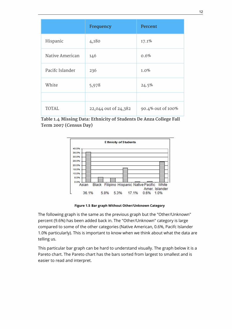
The table displays Ethnicity of Students but is missing the "Other/Unknown" category.This category contains people who did not feel they fit into any of the ethnicitycategories or declined to respond. Notice that the frequencies do not add up to thetotal number of students. Create a bar graph and not a pie chart.

Frequency Percent

Asian 8,794 36.1%

Black 1,412 5.8%

Filipino 1,298 5.3%

Table 1.4 Missing Data: Ethnicity of Students De Anza College FallTerm 2007 (Census Day)

11

Frequency Percent

Hispanic 4,180 17.1%

Native American 146 0.6%

Pacifc Islander 236 1.0%

White 5,978 24.5%

TOTAL 22,044 out of 24,382 90.4% out of 100%

Table 1.4 Missing Data: Ethnicity of Students De Anza College FallTerm 2007 (Census Day)

Figure 1.5 Bar graph Without Other/Unknown Category

The following graph is the same as the previous graph but the "Other/Unknown"percent (9.6%) has been added back in. The "Other/Unknown" category is largecompared to some of the other categories (Native American, 0.6%, Pacifc Islander1.0% particularly). This is important to know when we think about what the data aretelling us.

This particular bar graph can be hard to understand visually. The graph below it is aPareto chart. The Pareto chart has the bars sorted from largest to smallest and iseasier to read and interpret.

12

Figure 1.6 Bar Graph With Other/Unknown Category

Figure 1.7 Pareto Chart With Bars Sorted By Size

Pie Charts: No Missing Data

The following pie charts have the "Other/Unknown" category added back in (since thepercentages must add to 100%). The chart on the right is organized having the wedgesby size and makes for a more visually informative graph than the unsorted,alphabetical graph on the left.

Figure 1.8 Pie Charts with "Other/Unknown" category

13

1.5 Sampling and Data: Variation and Critical Evaluation

1.5.1 Variation in DataAvailable under Creative Commons-ShareAlike 4.0 International License (http://creativecommon


Variation is present in any set of data. For example, 16-ounce cans of beverage maycontain more or less than 16 ounces of liquid. In one study, eight 16 ounce cans weremeasured and produced the following amount (in ounces) of beverage:

15.8; 16.1; 15.2; 14.8; 15.8; 15.9; 16.0; 15.5

Measurements of the amount of beverage in a 16-ounce can may vary becausedifferent people make the measurements or because the exact amount, 16 ounces ofliquid, was not put into the cans. Manufacturers regularly run tests to determine if theamount of beverage in a 16-ounce can falls within the desired range.

Be aware that as you take data, your data may vary somewhat from the data someoneelse is taking for the same purpose. This is completely natural. However, if two ormore of you are taking the same data and get very different results, it is time for youand the others to reevaluate your data-taking methods and your accuracy.

1.5.2 Variation in SamplesAvailable under Creative Commons-ShareAlike 4.0 International License (http://creativecommon


It was mentioned previously that two or more samples from the same population,taken randomly, and having close to the same characteristics of the population aredifferent from each other. Suppose Doreen and Jung both decide to study the averageamount of time students at their college sleep each night. Doreen and Jung each takesamples of 500 students. Doreen uses systematic sampling and Jung uses clustersampling. Doreen's sample will be different from Jung's sample. Even if Doreen andJung used the same sampling method, in all likelihood their samples would bediferent. Neither would be wrong, however.

Think about what contributes to making Doreen's and Jung's samples diferent.

If Doreen and Jung took larger samples (i.e. the number of data values is increased),their sample results (the average amount of time a student sleeps) might be closer tothe actual population average. But still, their samples would be, in all likelihood,different from each other. This variability in samples cannot be stressed enough.

1.5.2.1 Size of a Sample

Available under Creative Commons-ShareAlike 4.0 International License (http://creativecommon


The size of a sample (often called the number of observations) is important. Theexamples you have seen in this book so far have been small. Samples of only a few

14










hundred observations, or even smaller, are sufcient for many purposes. In polling,samples that are from 1200 to 1500 observations are considered large enough andgood enough if the survey is random and is well done. You will learn why when youstudy confidence intervals.

Be aware that many large samples are biased. For example, call-in surveys areinvariable biased because people choose to respond or not.

1.5.2.2 Optional Collaborative Classroom Exercise



Exercise 1.5.1Divide into groups of two, three, or four. Your instructor will giveeach group one 6-sided die. Try this experiment twice. Roll one fairdie (6-sided) 20 times. Record the number of ones, twos, threes,fours, fves, and sixes you get below ("frequency" is the number oftimes a particular face of the die occurs):

Face on Die Frequency

1

2

3

4

5

6

Table 1.5 First Experiment (20 rolls)


1

2

Table 1.6 Second Experiment (20 rolls)

15





3

4

5

6

Table 1.6 Second Experiment (20 rolls)

Did the two experiments have the same results? Probably not. If youdid the experiment a third time, do you expect the results to beidentical to the first or second experiment? (Answer yes or no.) Whyor why not?

Which experiment had the correct results? They both did. The job ofthe statistician is to see through the variability and draw appropriateconclusions.

1.5.3 Critical EvaluationAvailable under Creative Commons-ShareAlike 4.0 International License (http://creativecommon


We need to critically evaluate the statistical studies we read about and analyze beforeaccepting the results of the study. Common problems to be aware of include

• Problems with Samples: A sample should be representative of the population. Asample that is not representative of the population is biased. Biased samples thatare not representative of the population give results that are inaccurate and notvalid.

• Self-Selected Samples: Responses only by people who choose to respond, such ascall-in surveys are often unreliable.

• Sample Size Issues: Samples that are too small may be unreliable. Larger samplesare better if possible. In some situations, small samples are unavoidable and canstill be used to draw conclusions, even though larger samples are better.Examples: Crash testing cars, medical testing for rare conditions.

• Undue infuence: Collecting data or asking questions in a way that infuences theresponse.

• Non-response or refusal of subject to participate: The collected responses may nolonger be representative of the population. Often, people with strong positive ornegative opinions may answer surveys, which can afect the results.

16




• Causality: A relationship between two variables does not mean that one causesthe other to occur. They may both be related (correlated) because of theirrelationship through a different variable.

• Self-Funded or Self-Interest Studies: A study performed by a person ororganization in order to support their claim. Is the study impartial? Read the studycarefully to evaluate the work. Do not automatically assume that the study isgood but do not automatically assume the study is bad either. Evaluate it on itsmerits and the work done.

• Misleading Use of Data: Improperly displayed graphs, incomplete data, lack ofcontext.

• Confounding: When the effects of multiple factors on a response cannot beseparated. Confounding makes it difficult or impossible to draw valid conclusionsabout the effect of each factor.

1.6 Sampling and Data: Frequency Relative Frequencyand Cumulative Frequency



Twenty students were asked how many hours they worked per day. Their responses,in hours, are listed below:

5; 6; 3; 3; 2; 4; 7; 5; 2; 3; 5; 6; 5; 4; 4; 3; 5; 2; 5; 3

Below is a frequency table listing the different data values in ascending order andtheir frequencies.

DATA VALUE FREQUENCY

2 3

3 5

4 3

5 6

6 2

7 1

Table 1.7 Frequency Table of Student Work Hours

A frequency is the number of times a given datum occurs in a data set. According tothe table above, there are three students who work 2 hours, five students who work 3

17




hours, etc. The total of the frequency column, 20, represents the total number ofstudents included in the sample.

A relative frequency is the fraction or proportion of times an answer occurs. To findthe relative frequencies, divide each frequency by the total number of students in thesample - in this case, 20. Relative frequencies can be written as fractions, percents, ordecimals.

DATA VALUE FREQUENCY RELATIVE FREQUENCY

2 3

3 5

4 3

5 6

6 2

7 1

Table 1.8 Frequency Table of Student Work Hours w/ RelativeFrequency

The sum of the relative frequency column is or 1.

Cumulative relative frequency is the accumulation of the previous relativefrequencies. To find the cumulative relative frequencies, add all the previous relativefrequencies to the relative frequency for the current row.

DATAVALUE

FREQUENCYRELATIVEFREQUENCY

CUMULATIVERELATIVE FREQUENCY

2 3 0.15

3 5 0.15+0.25=0.40

4 3 0.40+0.15=0.55

5 6 0.55+0.30=0.85

Table 1.9 Frequency Table of Student Work Hours w/ Relative andCumulative Relative Frequency

18

DATAVALUE


CUMULATIVERELATIVE FREQUENCY

6 2 0.85+0.10=0.95

7 1 0.95+0.05=1.00

Table 1.9 Frequency Table of Student Work Hours w/ Relative andCumulative Relative Frequency

The last entry of the cumulative relative frequency column is one, indicating that onehundred percent of the data has been accumulated.

Note: Because of rounding, the relative frequency column may not always sumto one and the last entry in the cumulative relative frequency column may notbe one. However, they each should be close to one.

The following table represents the heights, in inches, of a sample of 100 malesemiprofessional soccer players.

HEIGHT(INCHES)


CUMULATIVERELATIVEFREQUENCY

59.95 - 61.95 5 0.05

61.95 - 63.95 3 0.05+0.03=0.08

63.95 - 65.95 15 0.08+0.15=0.23

65.95 -67.95

40 0.23+0.40=0.63

67.95 -69.95

17 0.63+0.17=0.80

69.95 - 71.95 12 0.80+0.12=0.92

71.95 - 73.95 7 0.92+0.07=0.99

73.95 - 75.95 1 0.99+0.01=1.00

Total = 100 Total = 1.00

Table 1.10 Frequency Table of Soccer Player Height

The data in this table has been grouped into the following intervals:

19

• 59.95 - 61.95 inches• 61.95 - 63.95 inches• 63.95 - 65.95 inches• 65.95 - 67.95 inches• 67.95 - 69.95 inches• 69.95 - 71.95 inches• 71.95 - 73.95 inches• 73.95 - 75.95 inches

Note: This example is used again in the Descriptive Statistics (Section 2.1)chapter, where the method used to compute the intervals will be explained.

In this sample, there are 5 players whose heights are between 59.95 - 61.95 inches, 3players whose heights fall within the interval 61.95 - 63.95 inches, 15 players whoseheights fall within the interval 63.95 - 65.95 inches, 40 players whose heights fall withinthe interval 65.95 - 67.95 inches, 17 players whose heights fall within the interval 67.95- 69.95 inches, 12 players whose heights fall within the interval 69.95 - 71.95, 7 playerswhose height falls within the interval 71.95 - 73.95, and 1 player whose height fallswithin the interval 73.95 - 75.95. All heights fall between the endpoints of an intervaland not at the endpoints.

Example 1.6From the table, find the percentage of heights that are less than65.95 inches.

SolutionIf you look at the first, second, and third rows, the heights are all lessthan 65.95 inches. There are 5 + 3 + 15 = 23 males whose heights areless than 65.95 inches. The percentage of heights less than 65.95

inches is then or 23%. This percentage is the cumulative relativefrequency entry in the third row.

Example 1.7From the table, find the percentage of heights that fall between 61.95and 65.95 inches.

SolutionAdd the relative frequencies in the second and third rows: 0.03 + 0.15= 0.18 or 18%.

20

Example 1.8Use the table of heights of the 100 male semiprofessional soccerplayers. Fill in the blanks and check your answers.

1. The percentage of heights that are from 67.95 to 71.95 inches is:2. The percentage of heights that are from 67.95 to 73.95 inches is:3. The percentage of heights that are more than 65.95 inches is:4. The number of players in the sample who are between 61.95 and

71.95 inches tall is:5. What kind of data are the heights?6. Describe how you could gather this data (the heights) so that the

data are characteristic of all male semiprofessional soccer players.

Remember, you count frequencies. To find the relative frequency, divide thefrequency by the total number of data values. To find the cumulative relativefrequency, add all of the previous relative frequencies to the relative frequency for thecurrent row.



Exercise 1.6.1In your class, have someone conduct a survey of the number ofsiblings (brothers and sisters) each student has. Create a frequencytable. Add to it a relative frequency column and a cumulative relativefrequency column. Answer the following questions:

1. What percentage of the students in your class has 0 siblings?2. What percentage of the students has from 1 to 3 siblings?3. What percentage of the students has fewer than 3 siblings?

Example 1.9Nineteen people were asked how many miles, to the nearest milethey commute to work each day.

The data are as follows: 2; 5; 7; 3; 2; 10; 18; 15; 20; 7; 10; 18; 5; 12; 13;12; 4; 5; 10

The following table was produced:

DATA FREQUENCYRELATIVEFREQUENCY

CUMULATIVERELATIVEFREQUENCY

Table 1.11 Frequency of Commuting Distances

21




3 3 0.1579

4 1 0.2105

5 3 0.1579

7 2 0.2632

10 3 0.4737

12 2 0.7895

13 1 0.8421

15 1 0.8948

18 1 0.9474

20 1 1.0000

Table 1.11 Frequency of Commuting Distances

Problem1. Is the table correct? If it is not correct, what is wrong?2. True or False: Three percent of the people surveyed commute 3

miles. If the statement is not correct, what should it be? If thetable is incorrect, make the corrections.

3. What fraction of the people surveyed commute 5 or 7 miles?4. What fraction of the people surveyed commute 12 miles or more?

Less than 12 miles? Between 5 and 13 miles (does not include 5 and13 miles)?

1.6.2 Solutions to Exercises in Chapter 1Available under Creative Commons-ShareAlike 4.0 International License (http://creativecommon


Solution to Example 1.5, Problem

Items 1, 5, 11, and 12 are quantitative discrete; items 4, 6, 10, and 14 are quantitativecontinuous; and items 2, 3, 7, 8, 9, and 13 are qualitative.


1. 29%2. 36%

22




3. 77%4. 875. quantitative continuous6. get rosters from each team and choose a simple random sample from each


No. Frequency column sums to 18, not 19. Not all cumulative relative frequencies arecorrect.

1. False. Frequency for 3 miles should be 1; for 2 miles (left out), 2. Cumulativerelative frequency column should read: 0.1052, 0.1579, 0.2105, 0.3684, 0.4737,0.6316, 0.7368, 0.7895, 0.8421, 0.9474, 1.

2.

3.

23

Chapter 2 Descriptive Statistics

2.1 Descriptive Statistics: Introduction



Learning ObjectivesBy the end of this chapter, the student should be able to:

• Display data graphically and interpret graphs: stemplots, histogramsand boxplots.

• Recognize, describe, and calculate the measures of location of data:quartiles and percentiles.

• Recognize, describe, and calculate the measures of the center of data:mean, median, and mode.

• Recognize, describe, and calculate the measures of the spread of data:variance, standard deviation, and range.



Once you have collected data, what will you do with it? Data can be described andpresented in many different formats. For example, suppose you are interested inbuying a house in a particular area. You may have no clue about the house prices, soyou might ask your real estate agent to give you a sample data set of prices. Lookingat all the prices in the sample often is overwhelming. A better way might be to look atthe median price and the variation of prices. The median and variation are just twoways that you will learn to describe data. Your agent might also provide you with agraph of the data.

In this chapter, you will study numerical and graphical ways to describe and displayyour data. This area of statistics is called "Descriptive Statistics". You will learn tocalculate, and even more importantly, to interpret these measurements and graphs.

2.2 Descriptive Statistics: Displaying DataAvailable under Creative Commons-ShareAlike 4.0 International License (http://creativecommon


A statistical graph is a tool that helps you learn about the shape or distribution of asample. The graph can be a more effective way of presenting data than a mass of

24










numbers because we can see where data clusters and where there are only a few datavalues. Newspapers and the Internet use graphs to show trends and to enable readersto compare facts and figures quickly.

Statisticians often graph data first to get a picture of the data. Then, more formal toolsmay be applied.

Some of the types of graphs that are used to summarize and organize data are the dotplot, the bar chart, the histogram, the stem-and-leaf plot, the frequency polygon (atype of broken line graph), pie charts, and the boxplot. In this chapter, we will briefylook at stem-and-leaf plots, line graphs and bar graphs. Our emphasis will be onhistograms and boxplots.

2.3 Descriptive Statistics: HistogramAvailable under Creative Commons-ShareAlike 4.0 International License (http://creativecommon


For most of the work you do in this book, you will use a histogram to display the data.One advantage of a histogram is that it can readily display large data sets. A rule ofthumb is to use a histogram when the data set consists of 100 values or more.

A histogram consists of contiguous boxes. It has both a horizontal axis and a verticalaxis. The horizontal axis is labeled with what the data represents (for instance,distance from your home to school). The vertical axis is labeled either Frequency orrelative frequency. The graph will have the same shape with either label. Thehistogram (like the stemplot) can give you the shape of the data, the center, and thespread of the data. (The next section tells you how to calculate the center and thespread.)

The relative frequency is equal to the frequency for an observed value of the datadivided by the total number of data values in the sample. (In the chapter on Samplingand Data (Section 1.1), we defined frequency as the number of times an answeroccurs.) If:

• f = frequency• n = total number of data values (or the sum of the individual frequencies), and• RF = relative frequency,

then:

For example, if 3 students in Mr. Ahab's English class of 40 students received from90% to 100%, then,

Seven and a half percent of the students received 90% to 100%. Ninety percent to100% are quantitative measures.

25




To construct a histogram, first decide how many bars or intervals, also called classes,represent the data. Many histograms consist of from 5 to 15 bars or classes for clarity.Choose a starting point for the first interval to be less than the smallest data value. Aconvenient starting point is a lower value carried out to one more decimal placethan the value with the most decimal places. For example, if the value with the mostdecimal places is 6.1 and this is the smallest value, a convenient starting point is 6.05(6.1 - 0.05 = 6.05). We say that 6.05 has more precision. If the value with the mostdecimal places is 2.23 and the lowest value is 1.5, a convenient starting point is 1.495(1.5 - 0.005 = 1.495). If the value with the most decimal places is 3.234 and the lowestvalue is 1.0, a convenient starting point is 0.9995 (1.0 - .0005 = 0.9995). If all the datahappen to be integers and the smallest value is 2, then a convenient starting point is1.5 (2 - 0.5 = 1.5). Also, when the starting point and other boundaries are carried toone additional decimal place, no data value will fall on a boundary.

Example 2.1The following data are the heights (in inches to the nearest half inch)of 100 male semiprofessional soccer players. The heights arecontinuous data since height is measured.60; 60.5; 61; 61; 61.563.5; 63.5; 63.564; 64; 64; 64; 64; 64; 64; 64.5; 64.5; 64.5; 64.5; 64.5; 64.5; 64.5; 64.566; 66; 66; 66; 66; 66; 66; 66; 66; 66; 66.5; 66.5; 66.5; 66.5; 66.5; 66.5;66.5; 66.5; 66.5; 66.5; 66.5;67; 67; 67; 67; 67; 67; 67; 67; 67; 67; 67; 67; 67.5; 67.5; 67.5; 67.5;67.5; 67.5; 67.568; 68; 69; 69; 69; 69; 69; 69; 69; 69; 69; 69; 69.5; 69.5; 69.5; 69.5; 69.570; 70; 70; 70; 70; 70; 70.5; 70.5; 70.5; 71; 71; 7172; 72; 72; 72.5; 72.5; 73; 73.574The smallest data value is 60. Since the data with the most decimalplaces has one decimal (for instance, 61.5), we want our starting pointto have two decimal places. Since the numbers 0.5, 0.05, 0.005, etc.are convenient numbers, use 0.05 and subtract it from 60, thesmallest value, for the convenient starting point.60 - 0.05 = 59.95 which is more precise than, say, 61.5 by one decimalplace. The starting point is, then, 59.95.

The largest value is 74. 74 + 0.05 = 74.05 is the ending value.

Next, calculate the width of each bar or class interval. To calculatethis width, subtract the starting point from the ending value anddivide by the number of bars (you must choose the number of barsyou desire). Suppose you choose 8 bars.

26

Note: We will round up to 2 and make each bar or class interval 2 unitswide. Rounding up to 2 is one way to prevent a value from falling on aboundary. Rounding to the next number is necessary even if it goesagainst the standard rules of rounding. For this example, using 1.76 asthe width would also work.

The boundaries are:

• 59.95• 59.95 + 2 = 61.95• 61.95 + 2 = 63.95• 63.95 + 2 = 65.95• 65.95 + 2 = 67.95• 67.95 + 2 = 69.95• 69.95 + 2 = 71.95• 71.95 + 2 = 73.95• 73.95 + 2 = 75.95

The heights 60 through 61.5 inches are in the interval 59.95 - 61.95.The heights that are 63.5 are in the interval 61.95 - 63.95. The heightsthat are 64 through 64.5 are in the interval 63.95 - 65.95. The heights66 through 67.5 are in the interval 65.95 - 67.95. The heights 68through 69.5 are in the interval 67.95 - 69.95. The heights 70 through71 are in the interval 69.95 - 71.95. The heights 72 through 73.5 are inthe interval 71.95 - 73.95. The height 74 is in the interval 73.95 -75.95.

The following histogram displays the heights on the x-axis andrelative frequency on the y-axis.

27

Example 2.2The following data are the number of books bought by 50 part-timecollege students at ABC College. The number of books is discrete datasince books are counted.

1; 1; 1; 1; 1; 1; 1; 1; 1; 1; 12; 2; 2; 2; 2; 2; 2; 2; 2; 23; 3; 3; 3; 3; 3; 3; 3; 3; 3; 3; 3; 3; 3; 3; 34; 4; 4; 4; 4; 45; 5; 5; 5; 56; 6

Eleven students buy 1 book. Ten students buy 2 books. Sixteenstudents buy 3 books. Six students buy 4 books. Five students buy 5books. Two students buy 6 books.

Because the data are integers, subtract 0.5 from 1, the smallest datavalue and add 0.5 to 6, the largest data value. Then the starting pointis 0.5 and the ending value is 6.5.

ProblemNext, calculate the width of each bar or class interval. If the data arediscrete and there are not too many different values, a width thatplaces the data values in the middle of the bar or class interval is themost convenient. Since the data consist of the numbers 1, 2, 3, 4, 5, 6and the starting point is 0.5, a width of one places the 1 in the middleof the interval from 0.5 to 1.5, the 2 in the middle of the interval from1.5 to 2.5, the 3 in the middle of the interval from 2.5 to 3.5, the 4 inthe middle of the interval from ______ to ______, the 5 in themiddle of the interval from to ______, and the ______in the middleof the interval from ______to ______ .

Calculate the number of bars as follows:

where 1 is the width of a bar. Therefore, bars = 6.

The following histogram displays the number of books on the x-axisand the frequency on the y-axis.

28

Using the TI-83, 83+, 84, 84+ Calculator Instructions

Go to the Appendix (14:Appendix) in the menu on the left. There are calculatorinstructions for entering data and for creating a customized histogram. Create thehistogram for Example 2.

• Press Y=. Press CLEAR to clear out any equations.• Press STAT 1:EDIT. If L1 has data in it, arrow up into the name L1, press CLEAR

and arrow down. If necessary, do the same for L2.• Into L1, enter 1, 2, 3, 4, 5, 6• Into L2, enter 11, 10, 16, 6, 5, 2• Press WINDOW. Make Xmin = .5, Xmax = 6.5, Xscl = (6.5 -.5)/6, Ymin = -1, Ymax =

20, Yscl = 1, Xres = 1• Press 2nd Y =. Start by pressing 4:Plotsof ENTER.• Press 2nd Y =. Press 1:Plot1. Press ENTER. Arrow down to TYPE. Arrow to the 3rd

picture (histogram). Press ENTER.• Arrow down to Xlist: Enter L1 (2nd 1). Arrow down to Freq. Enter L2 (2nd 2).• Press GRAPH• Use the TRACE key and the arrow keys to examine the histogram.

2.3.1 Optional Collaborative ExerciseAvailable under Creative Commons-ShareAlike 4.0 International License (http://creativecommon


Count the money (bills and change) in your pocket or purse. Your instructor will recordthe amounts. As a class, construct a histogram displaying the data. Discuss how manyintervals you think is appropriate. You may want to experiment with the number ofintervals. Discuss, also, the shape of the histogram.

Record the data, in dollars (for example, 1.25 dollars).

Construct a histogram.

29




2.4 Descriptive Statistics: Measuring the Center of theData



The "center" of a data set is also a way of describing location. The two most widelyused measures of the "center" of the data are the mean (average) and the median. Tocalculate the mean weight of 50 people, add the 50 weights together and divide by50. To find the median weight of the 50 people, order the data and find the numberthat splits the data into two equal parts (previously discussed under box plots in thischapter). The median is generally a better measure of the center when there areextreme values or outliers because it is not affected by the precise numerical values ofthe outliers. The mean is the most common measure of the center.

Note: The words "mean" and "average" are often used interchangeably. Thesubstitution of one word for the other is common practice. The technical termis "arithmetic mean" and "average" is technically a center location. However,in practice among non-statisticians, "average" is commonly accepted for"arithmetic mean."

The mean can also be calculated by multiplying each distinct value by its frequencyand then dividing the sum by the total number of data values. The letter used torepresent the sample mean is an x with a bar over it (pronounced "x bar"): .

The Greek letter µ (pronounced "mew") represents the population mean. One of therequirements for the sample mean to be a good estimate of the population mean isfor the sample taken to be truly random.

To see that both ways of calculating the mean are the same, consider the sample:

1; 1; 1; 2; 2; 3; 4; 4; 4; 4; 4

In the second calculation for the sample mean, the frequencies are 3, 2, 1, and 5. You

can quickly find the location of the median by using the expression .

The letter n is the total number of data values in the sample. If n is an odd number,the median is the middle value of the ordered data (ordered smallest to largest). If n isan even number, the median is equal to the two middle values added together anddivided by 2 after the data has been ordered. For example, if the total number of data

values is 97, then . The median is the 49th value in theordered data. If the total number of data values is 100, then

. The median occurs midway between the 50th and 51st

30




values. The location of the median and the value of the median are not the same. Theupper case letter M is often used to represent the median. The next exampleillustrates the location of the median and the value of the median.

Example 2.3AIDS data indicating the number of months an AIDS patient livesafter taking a new antibody drug are as follows (smallest to largest):

3; 4; 8; 8; 10; 11; 12; 13; 14; 15; 15; 16; 16; 17; 17; 18; 21; 22; 22; 24; 24; 25;26; 26; 27; 27; 29; 29; 31; 32; 33; 33; 34; 34; 35; 37; 40; 44; 44; 47

Calculate the mean and the median.

SolutionThe calculation for the mean is:

To find the median, M, first use the formula for the location. Thelocation is:

Starting at the smallest value, the median is located between the20th and 21st values (the two 24s):3; 4; 8; 8; 10; 11; 12; 13; 14; 15; 15; 16; 16; 17; 17; 18; 21; 22; 22; 24; 24; 25;26; 26; 27; 27; 29; 29; 31; 32; 33; 33; 34; 34; 35; 37; 40; 44; 44; 47

The median is 24.

Using the TI-83, 83+, 84, 84+ Calculators

Calculator Instructions are located in the menu item 14:Appendix (Notes for the TI-83,83+, 84, 84+ Calculators).

• Enter data into the list editor. Press STAT 1:EDIT• Put the data values in list L1.• Press STAT and arrow to CALC. Press 1:1-VarStats. Press 2nd 1 for L1 and ENTER.• Press the down and up arrow keys to scroll.

31

Example 2.4Suppose that, in a small town of 50 people, one person earns$5,000,000 per year and the other 49 each earn $30,000. Which is thebetter measure of the "center," the mean or the median?

Solution

(There are 49 people who earn $30,000 and one person who earns$5,000,000.)The median is a better measure of the "center" than the meanbecause 49 of the values are 30,000 and one is 5,000,000. The5,000,000 is an outlier. The 30,000 gives us a better sense of themiddle of the data.Another measure of the center is the mode. The mode is the mostfrequent value. If a data set has two values that occur the samenumber of times, then the set is bimodal.

Example 2.5Statistics exam scores for 20 students are as follows:

50 ; 53 ; 59 ; 59 ; 63 ; 63 ; 72 ; 72 ; 72 ; 72 ; 72 ; 76 ; 78 ; 81 ; 83 ; 84 ; 84 ;84 ; 90 ; 93

ProblemFind the mode.

SolutionThe most frequent score is 72, which occurs five times. Mode 72.

Example 2.6Five real estate exam scores are 430, 430, 480, 480, 495. The data setis bimodal because the scores 430 and 480 each occur twice.

When is the mode the best measure of the "center"? Consider aweight loss program that advertises a mean weight loss of six poundsthe first week of the program. The mode might indicate that mostpeople lose two pounds the first week, making the program lessappealing.

32

Note: The mode can be calculated for qualitative data as well as forquantitative data.

Statistical software will easily calculate the mean, the median, andthe mode. Some graphing calculators can also make thesecalculations. In the real world, people make these calculations usingsoftware.

2.4.1 The Law of Large Numbers and the MeanAvailable under Creative Commons-ShareAlike 4.0 International License (http://creativecommon


The Law of Large Numbers says that if you take samples of larger and larger size fromany population, then the mean of the sample is very likely to get closer and closer toµ. This is discussed in more detail in The Central Limit Theorem.

Note: The formula for the mean is located in the Summary of Formulas sectioncourse.

2.4.2 Sampling Distributions and Statistic of a SamplingDistribution



You can think of a sampling distribution as a relative frequency distribution with agreat many samples. (See Sampling and Data for a review of relative frequency).Suppose thirty randomly selected students were asked the number of movies theywatched the previous week. The results are in the relative frequency table shownbelow.

# of movies Relative Frequency

0 5/30

1 15/30

2 6/30

3 4/30

4 1/30

33







If you let the number of samples get very large (say, 300 million or more), therelative frequency table becomes a relative frequency distribution.

A statistic is a number calculated from a sample. Statistic examples include the mean,the median and the mode as well as others. The sample mean is an example of astatistic which estimates the population mean µ.

2.5 Descriptive Statistics: Skewness and the Mean,Median, and Mode



Consider the following data set:

4 ; 5 ; 6 ; 6 ; 6 ; 7 ; 7 ; 7 ; 7 ; 7 ; 7 ; 8 ; 8 ; 8 ; 9 ; 10

This data set produces the histogram shown below. Each interval has width one andeach value is located in the middle of an interval.

The histogram displays a symmetrical distribution of data. A distribution issymmetrical if a vertical line can be drawn at some point in the histogram such thatthe shape to the left and the right of the vertical line are mirror images of each other.The mean, the median, and the mode are each 7 for these data. In a perfectlysymmetrical distribution, the mean and the median are the same. This examplehas one mode (unimodal) and the mode is the same as the mean and median. In asymmetrical distribution that has two modes (bimodal), the two modes would bedifferent from the mean and median.

The histogram for the data:

4 ; 5 ; 6 ; 6 ; 6 ; 7 ; 7 ; 7 ; 7 ; 8

is not symmetrical. The right-hand side seems "chopped off" compared to the leftside. The shape distribution is called skewed to the left because it is pulled out to theleft.

34




The mean is 6.3, the median is 6.5, and the mode is 7. Notice that the mean is lessthan the median and they are both less than the mode. The mean and the medianboth reflect the skewing but the mean more so.

The histogram for the data:

6 ; 7 ; 7 ; 7 ; 7 ; 8 ; 8 ; 8 ; 9 ; 10

is also not symmetrical. It is skewed to the right.

The mean is 7.7, the median is 7.5, and the mode is 7. Of the three statistics, themean is the largest, while the mode is the smallest. Again, the mean refects theskewing the most.

To summarize, generally if the distribution of data is skewed to the left, the mean isless than the median, which is often less than the mode. If the distribution of data isskewed to the right, the mode is often less than the median, which is less than themean.

Skewness and symmetry become important when we discuss probability distributionsin later chapters.

35

2.6 Descriptive Statistics: Measuring the Spread of theData



An important characteristic of any set of data is the variation in the data. In some datasets, the data values are concentrated closely near the mean; in other data sets, thedata values are more widely spread out from the mean. The most common measureof variation, or spread, is the standard deviation.

The standard deviation is a number that measures how far data values are fromtheir mean. The standard deviation

• provides a numerical measure of the overall amount of variation in a data set• can be used to determine whether a particular data value is close to or far from

the mean

The standard deviation provides a measure of the overall variation in a data set

The standard deviation is always positive or 0. The standard deviation is small whenthe data are all concentrated close to the mean, exhibiting little variation or spread.The standard deviation is larger when the data values are more spread out from themean, exhibiting more variation.

Suppose that we are studying waiting times at the checkout line for customers atsupermarket A and supermarket B; the average wait time at both markets is 5minutes. At market A, the standard deviation for the waiting time is 2 minutes; atmarket B the standard deviation for the waiting time is 4 minutes.

Because market B has a higher standard deviation, we know that there is morevariation in the waiting times at market B. Overall, wait times at market B are morespread out from the average; wait times at market A are more concentrated near theaverage.

The standard deviation can be used to determine whether a data value is closeto or far from the mean.

Suppose that Rosa and Binh both shop at Market A. Rosa waits for 7 minutes and Binhwaits for 1 minute at the checkout counter. At market A, the mean wait time is 5minutes and the standard deviation is 2 minutes. The standard deviation can be usedto determine whether a data value is close to or far from the mean.

Rosa waits for 7 minutes:

• 7 is 2 minutes longer than the average of 5; 2 minutes is equal to one standarddeviation.

• Rosa's wait time of 7 minutes is 2 minutes longer than the average of 5minutes.

• Rosa's wait time of 7 minutes is one standard deviation above the average of 5minutes.

36




Binh waits for 1 minute.

• 1 is 4 minutes less than the average of 5; 4 minutes is equal to two standarddeviations.

• Binh's wait time of 1 minute is 4 minutes less than the average of 5 minutes.• Binh's wait time of 1 minute is two standard deviations below the average of 5

minutes.• A data value that is two standard deviations from the average is just on the

borderline for what many statisticians would consider to be far from the average.Considering data to be far from the mean if it is more than 2 standard deviationsaway is more of an approximate "rule of thumb" than a rigid rule. In general, theshape of the distribution of the data afects how much of the data is further awaythan 2 standard deviations. (We will learn more about this in later chapters.)

The number line may help you understand standard deviation. If we were to put 5 and7 on a number line, 7 is to the right of 5. We say, then, that 7 is one standard deviationto the right of 5 because 5 + (1)(2) = 7.

If 1 were also part of the data set, then 1 is two standard deviations to the left of 5because 5 + (−2)(2) = 1.

• In general, a value = mean + (#ofSTDEV)(standard deviation)• where #ofSTDEVs = the number of standard deviations• 7 is one standard deviation more than the mean of 5 because: 7 = 5 + (1)(2)• 1 is two standard deviations less than the mean of 5 because: 1 = 5 + (−2)(2)

The equation value = mean + (#ofSTDEVs)(standard deviation) can be expressed fora sample and for a population:

• sample:• Population:

The lower case letter s represents the sample standard deviation and the Greek letterσ (sigma, lower case) represents the population standard deviation.

The symbol is the sample mean and the Greek symbol µ is the population mean.

Calculating the Standard Deviation

If x is a number, then the diference "x - mean" is called its deviation. In a data set,there are as many deviations as there are items in the data set. The deviations areused to calculate the standard deviation. If the numbers belong to a population, insymbols a deviation is x − µ . For sample data, in symbols a deviation is .

37

The procedure to calculate the standard deviation depends on whether the numbersare the entire population or are data from a sample. The calculations are similar, butnot identical. Therefore the symbol used to represent the standard deviation dependson whether it is calculated from a population or a sample. The lower case letter srepresents the sample standard deviation and the Greek letter σ (sigma, lower case)represents the population standard deviation. If the sample has the samecharacteristics as the population, then s should be a good estimate of σ.

To calculate the standard deviation, we need to calculate the variance first. Thevariance is an average of the squares of the deviations (the values for a

sample, or the x − µ values for a population). The symbol σ2 represents the populationvariance; the population standard deviation σ is the square root of the population

variance. The symbol s2 represents the sample variance; the sample standarddeviation s is the square root of the sample variance. You can think of the standarddeviation as a special average of the deviations.

If the numbers come from a census of the entire population and not a sample, whenwe calculate the average of the squared deviations to find the variance, we divide byN, the number of items in the population. If the data are from a sample rather than apopulation, when we calculate the average of the squared deviations, we divide byn-1, one less than the number of items in the sample. You can see that in the formulasbelow.

Formulas for the Sample Standard Deviation

• or• For the sample standard deviation, the denominator is n-1, that is the sample size

MINUS 1.

Formulas for the Population Standard Deviation

• or

• For the population standard deviation, the denominator is N, the number ofitems in the population.

In these formulas, f represents the frequency with which a value appears. Forexample, if a value appears once, f is 1. If a value appears three times in the data setor population, f is 3.

Sampling Variability of a Statistic

The statistic of a sampling distribution was discussed in Descriptive Statistics:Measuring the Center of the Data. How much the statistic varies from one sampleto another is known as the sampling variability of a statistic. You typically measurethe sampling variability of a statistic by its standard error. The standard error of themean is an example of a standard error. It is a special standard deviation and isknown as the standard deviation of the sampling distribution of the mean. You willcover the standard error of the mean in The Central Limit Theorem (not now). The

38

notation for the standard error of the mean is where σ is the standard deviationof the population and n is the size of the sample.

Note: In practice, USE A CALCULATOR OR COMPUTER SOFTWARE TOCALCULATE THE STANDARD DEVIATION. If you are using a TI-83,83+,84+calculator, you need to select the appropriate standard deviation σx or sx

from the summary statistics. We will concentrate on using and interpretingthe information that the standard deviation gives us. However you shouldstudy the following step-by-step example to help you understand how thestandard deviation measures variation from the mean.

Example 2.7In a fifth grade class, the teacher was interested in the average ageand the sample standard deviation of the ages of her students. Thefollowing data are the ages for a SAMPLE of n = 20 fifth gradestudents. The ages are rounded to the nearest half year:

9 ; 9.5 ; 9.5 ; 10 ; 10 ; 10 ; 10 ; 10.5 ; 10.5 ; 10.5 ; 10.5 ; 11 ; 11 ; 11 ; 11 ; 11 ;11 ; 11.5 ; 11.5 ; 11.5

The average age is 10.53 years, rounded to 2 places.

The variance may be calculated by using a table. Then the standarddeviation is calculated by taking the square root of the variance. Wewill explain the parts of the table after calculatings.

Data Freq. Deviations Deviations2 (Freq.)(Deviations2)

x f

9 19 − 10.525= −1.525

(−1.525)2 =2.325625

1 × 2.325625 =2.325625

9.5 29.5 −10.525 =−1.025

(−1.025)2 =1.050625

2 × 1.050625 =2.101250

10 410 − 10.525= −0.525

(−0.525)2 =0.275625

4 × .275625 = 1.1025

39

Data Freq. Deviations Deviations2 (Freq.)(Deviations2)

10.5 410.5 −10.525 =−0.025

(−0.025)2 =0.000625

4 × .000625 = .0025

11 611 − 10.525= 0.475

(0.475)2 =0.225625

6 × .225625 = 1.35375

11.5 311.5 −10.525 =0.975

(0.975)2 =0.950625

3 × .950625 =2.851875

The sample variance, s2, is equal to the sum of the last column(9.7375) divided by the total number of data values minus one (20 -1):

The sample standard deviation s is equal to the square root of thesample variance:

Rounded to two decimal places, s =0.72

Typically, you do the calculation for the standard deviation on yourcalculator or computer. The intermediate results are not rounded.This is done for accuracy.

Problem 1Verify the mean and standard deviation calculated above on yourcalculator or computer.

Solution

Using the TI-83,83+,84+ Calculators

• Enter data into the list editor. Press STAT 1:EDIT. If necessary,clear the lists by arrowing up into the name. Press CLEAR andarrow down.

40

• Put the data values (9, 9.5, 10, 10.5, 11, 11.5) into list L1 and thefrequencies (1, 2, 4, 4, 6, 3) into list L2. Use the arrow keys to movearound.

• Press STAT and arrow to CALC. Press 1:1-VarStats and enter L1(2nd 1), L2 (2nd 2). Do not forget the comma. Press ENTER.

•• Use Sx because this is sample data (not a population): Sx =

0.715891• For the following problems, recall that value = mean +

(#ofSTDEVs)(standard deviation)• For a sample:• For a population:• For this example, use because the

data is from a sample

Problem 2Find the value that is 1 standard deviation above the mean. Find

Solution

Problem 3Find the value that is two standard deviations below the mean. Find

Solution

Problem 4Find the values that are 1.5 standard deviations from (below andabove) the mean.

Solution

Explanation of the standard deviation calculation shown in the table

The deviations show how spread out the data are about the mean. The data value11.5 is farther from the mean than is the data value 11. The deviations 0.97 and 0.47indicate that. A positive deviation occurs when the data value is greater than themean. A negative deviation occurs when the data value is less than the mean; thedeviation is -1.525 for the data value 9. If you add the deviations, the sum is alwayszero. (For this example, there are n=20 deviations.) So you cannot simply add the

41

deviations to get the spread of the data. By squaring the deviations, you make thempositive numbers, and the sum will also be positive. The variance, then, is the averagesquared deviation.

The variance is a squared measure and does not have the same units as the data.Taking the square root solves the problem. The standard deviation measures thespread in the same units as the data.

Notice that instead of dividing by n=20, the calculation divided by n-1=20-1=19because the data is a sample. For the sample variance, we divide by the sample sizeminus one (n − 1). Why not divide by n? The answer has to do with the populationvariance. The sample variance is an estimate of the population variance. Basedon the theoretical mathematics that lies behind these calculations, dividing by (n − 1)gives a better estimate of the population variance.

Note: Your concentration should be on what the standard deviation tells usabout the data. The standard deviation is a number which measures how farthe data are spread from the mean. Let a calculator or computer do thearithmetic.

The standard deviation, s or σ, is either zero or larger than zero. When the standarddeviation is 0, there is no spread; that is, the all the data values are equal to eachother. The standard deviation is small when the data are all concentrated close to themean, and is larger when the data values show more variation from the mean. Whenthe standard deviation is a lot larger than zero, the data values are very spread outabout the mean; outliers can make s or σ very large.

The standard deviation, when first presented, can seem unclear. By graphing yourdata, you can get a better "feel" for the deviations and the standard deviation. You willfind that in symmetrical distributions, the standard deviation can be very helpful butin skewed distributions, the standard deviation may not be much help. The reason isthat the two sides of a skewed distribution have different spreads. In a skeweddistribution, it is better to look at the first quartile, the median, the third quartile, thesmallest value, and the largest value. Because numbers can be confusing, alwaysgraph your data.

Note: The formula for the standard deviation is at the end of the chapter.

Example 2.8Use the following data (first exam scores) from Susan Dean's springpre-calculus class:

33; 42; 49; 49; 53; 55; 55; 61; 63; 67; 68; 68; 69; 69; 72; 73; 74; 78; 80;83; 88; 88; 88; 90; 92; 94; 94; 94; 94; 96; 100

1. Create a chart containing the data, frequencies, relativefrequencies, and cumulative relative frequencies to three decimalplaces.

2. Calculate the following to one decimal place using a TI-83+ orTI-84 calculator:

42

1. The sample mean2. The sample standard deviation3. The median4. The first quartile5. The third quartile6. IQR

3. Construct a box plot and a histogram on the same set of axes.Make comments about the box plot, the histogram, and the chart.

Solution

1.

Data FrequencyRelativeFrequency

CumulativeRelativeFrequency

33 1 0.032 0.032

42 1 0.032 0.064

49 2 0.065 0.129

53 1 0.032 0.161

55 2 0.065 0.226

61 1 0.032 0.258

63 1 0.032 0.29

67 1 0.032 0.322

68 2 0.065 0.387

69 2 0.065 0.452

72 1 0.032 0.484

73 1 0.032 0.516

74 1 0.032 0.548

43

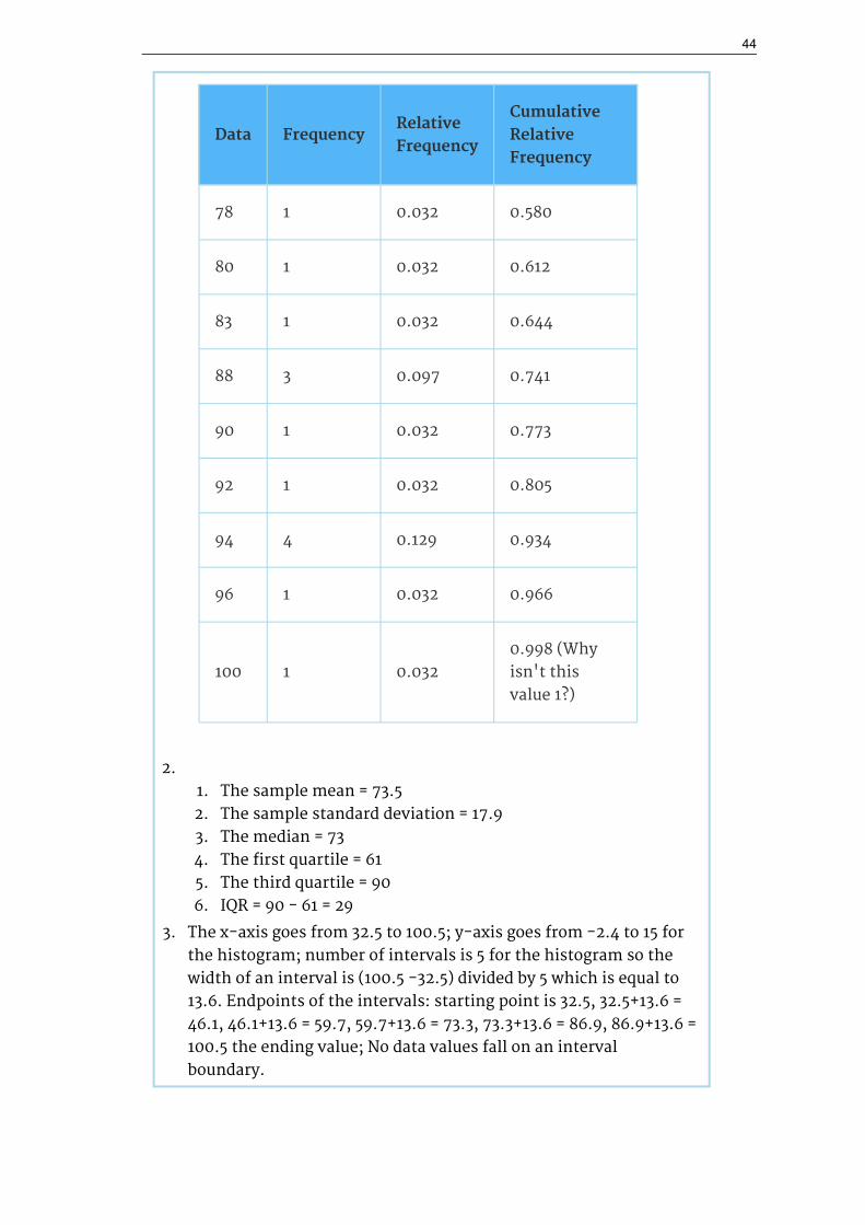
Data FrequencyRelativeFrequency

CumulativeRelativeFrequency

78 1 0.032 0.580

80 1 0.032 0.612

83 1 0.032 0.644

88 3 0.097 0.741

90 1 0.032 0.773

92 1 0.032 0.805

94 4 0.129 0.934

96 1 0.032 0.966

100 1 0.0320.998 (Whyisn't thisvalue 1?)

2.1. The sample mean = 73.52. The sample standard deviation = 17.93. The median = 734. The first quartile = 615. The third quartile = 906. IQR = 90 - 61 = 29

3. The x-axis goes from 32.5 to 100.5; y-axis goes from -2.4 to 15 forthe histogram; number of intervals is 5 for the histogram so thewidth of an interval is (100.5 -32.5) divided by 5 which is equal to13.6. Endpoints of the intervals: starting point is 32.5, 32.5+13.6 =46.1, 46.1+13.6 = 59.7, 59.7+13.6 = 73.3, 73.3+13.6 = 86.9, 86.9+13.6 =100.5 the ending value; No data values fall on an intervalboundary.

44

The long left whisker in the box plot is refected in the left side of thehistogram. The spread of the exam scores in the lower 50% is greater(73 - 33 = 40) than the spread in the upper 50% (100 - 73 = 27). Thehistogram, box plot, and chart all refect this. There are a substantialnumber of A and B grades (80s, 90s, and 100). The histogram clearlyshows this. The box plot shows us that the middle 50% of the examscores (IQR = 29) are Ds, Cs, and Bs. The box plot also shows us thatthe lower 25% of the exam scores are Ds and Fs.

Comparing Values from Different Data Sets

The standard deviation is useful when comparing data values that come fromdifferent data sets. If the data sets have different means and standard deviations, itcan be misleading to compare the data values directly.

• For each data value, calculate how many standard deviations the value is awayfrom its mean.

• Use the formula: value = mean + (#ofSTDEVs)(standard deviation); solve for#ofSTDEVs.

• Compare the results of this calculation.

#ofSTDEVs is often called a "z-score"; we can use the symbol z. In symbols, theformulas become:

Sample

Population

45

Example 2.9Two students, John and Ali, from different high schools, wanted tofind out who had the highest G.P.A. when compared to his school.Which student had the highest G.P.A. when compared to his school?

Student GPASchoolMean GPA

School StandardDeviation

John 2.85 3.0 0.7

Ali 77 80 10

Solution

For each student, determine how many standard deviations(#ofSTDEVs) his GPA is away from the average, for his school. Paycareful attention to signs when comparing and interpreting theanswer.

John has the better G.P.A. when compared to his school because hisG.P.A. is 0.21 standard deviations below his school's mean whileAli's G.P.A. is 0.3 standard deviations below his school's mean.

John's z-score of −0.21 is higher than Ali's z-score of −0.3 . For GPA,higher values are better, so we conclude that John has the better GPAwhen compared to his school.

The following lists give a few facts that provide a little more insight into what thestandard deviation tells us about the distribution of the data.

For ANY data set, no matter what the distribution of the data is:

• At least 75% of the data is within 2 standard deviations of the mean.• At least 89% of the data is within 3 standard deviations of the mean.• At least 95% of the data is within 4 1/2 standard deviations of the mean.• This is known as Chebyshev's Rule.

For data having a distribution that is MOUND-SHAPED and SYMMETRIC:

• Approximately 68% of the data is within 1 standard deviation of the mean.

46

• Approximately 95% of the data is within 2 standard deviations of the mean.• More than 99% of the data is within 3 standard deviations of the mean.• This is known as the Empirical Rule.• It is important to note that this rule only applies when the shape of the

distribution of the data is mound-shaped and symmetric. We will learn moreabout this when studying the "Normal" or "Gaussian" probability distribution inlater chapters.

**With contributions from Roberta Bloom




• 3.5 to 4.5• 4.5 to 5.5• 6• 5.5 to 6.5

47




Chapter 3 The Normal Distribution

3.1 Normal Distribution: Introduction




• Recognize the normal probability distribution and apply itappropriately.

• Recognize the standard normal probability distribution and apply itappropriately.

• Compare normal probabilities by converting to the standard normaldistribution.



The normal, a continuous distribution, is the most important of all the distributions. Itis widely used and even more widely abused. Its graph is bell-shaped. You see the bellcurve in almost all disciplines. Some of these include psychology, business, economics,the sciences, nursing, and, of course, mathematics. Some of your instructors may usethe normal distribution to help determine your grade. Most IQ scores are normallydistributed. Often real estate prices ft a normal distribution. The normal distribution isextremely important but it cannot be applied to everything in the real world.

In this chapter, you will study the normal distribution, the standard normal, andapplications associated with them.

3.1.3 Optional Collaborative Classroom ActivityAvailable under Creative Commons-ShareAlike 4.0 International License (http://creativecommon


Your instructor will record the heights of both men and women in your class,separately. Draw histograms of your data. Then draw a smooth curve through eachhistogram. Is each curve somewhat bell-shaped? Do you think that if you hadrecorded 200 data values for men and 200 for women that the curves would look bell-shaped? Calculate the mean for each data set. Write the means on the x-axis of theappropriate graph below the peak. Shade the approximate area that represents theprobability that one randomly chosen male is taller than 72 inches. Shade the

48










approximate area that represents the probability that one randomly chosen female isshorter than 60 inches. If the total area under each curve is one, does eitherprobability appear to be more than 0.5?

The normal distribution has two parameters (two numerical descriptive measures),the mean (µ) and the standard deviation (σ). If X is a quantity to be measured that hasa normal distribution with mean (µ) and the standard deviation (σ), we designate thisby writing

The probability density function is a rather complicated function. Do not memorize it.It is not necessary.

The cumulative distribution function is P (X<x) . It is calculated either by a calculator ora computer or it is looked up in a table. Technology has made the tables basicallyobsolete. For that reason, as well as the fact that there are various table formats, weare not including table instructions in this chapter. See the NOTE in this chapter inCalculation of Probabilities.

The curve is symmetrical about a vertical line drawn through the mean, µ. In theory,the mean is the same as the median since the graph is symmetric about µ. As thenotation indicates, the normal distribution depends only on the mean and thestandard deviation. Since the area under the curve must equal one, a change in thestandard deviation, σ, causes a change in the shape of the curve; the curve becomesfatter or skinnier depending on σ. A change in µ causes the graph to shift to the left orright. This means there are an infnite number of normal probability distributions. Oneof special interest is called the standard normal distribution.

3.2 Normal Distribution: Standard Normal DistributionAvailable under Creative Commons-ShareAlike 4.0 International License (http://creativecommon


The standard normal distribution is a normal distribution of standardized valuescalled z-scores. A z-score is measured in units of the standard deviation. Forexample, if the mean of a normal distribution is 5 and the standard deviation is 2, thevalue 11 is 3 standard deviations above (or to the right of) the mean. The calculationis:

49




The z-score is 3.

The mean for the standard normal distribution is 0 and the standard deviation is 1.

The transformation produces the distribution Z∼ N (0, 1) . The value xcomes from a normal distribution with mean µ and standard deviation σ.

3.3 Normal Distribution: Z-scoresAvailable under Creative Commons-ShareAlike 4.0 International License (http://creativecommon


If X is a normally distributed random variable and X∼N(µ, σ), then the z-score is:

The z-score tells you how many standard deviations that the value x is above (tothe right of) or below (to the left of) the mean, µ. Values of x that are larger thanthe mean have positive z-scores and values of x that are smaller than the mean havenegative z-scores. If x equals the mean, then x has a z-score of 0.

Example 3.1Suppose X∼∼N (5, 6). This says that X is a normally distributedrandom variable with mean µ = 5 and standard deviation σ = 6.Suppose x = 17. Then:

This means that x = 17 is 2 standard deviations (2σ) above or to theright of the mean µ = 5. The standard deviation is σ = 6.Notice that:

5+2 · 6 = 17 (The pattern is µ + zσ = x.)

Now suppose x = 1. Then:

(rounded to two decimal places)

This means that x = 1 is 0.67 standard deviations (− 0.67σ) below orto the left of the mean µ = 5. Notice that:

5+(−0.67) (6) is approximately equal to 1 (This has the pattern µ+(−0.67) σ = 1 ) Summarizing, when z is positive, x is above or to theright of µ and when z is negative, x is to the left of or below µ.

50




Example 3.2Some doctors believe that a person can lose 5 pounds, on the average,in a month by reducing his/her fat intake and by exercisingconsistently. Suppose weight loss has a normal distribution. Let X =the amount of weight lost (in pounds) by a person in a month. Use astandard deviation of 2 pounds. X∼∼N (5, 2). Fill in the blanks.

Problem 1Suppose a person lost 10 pounds in a month. The z-score when x = 10pounds is z = 2.5 (verify). This z-score tells you that x = 10 is________ standard deviations to the ________ (right or left) of themean ________ ( What is the mean?).

Problem 2Suppose a person gained 3 pounds (a negative weight loss). Then z________. This z-score tells you that x = −3 is ________ standarddeviations to the ________ (right or left) of the mean.

Suppose the random variables X and Y have the following normaldistributions: X ∼ N (5, 6) and Y ∼ N (2, 1). If x = 17, then z = 2. (Thiswas previously shown.) If y = 4, what is z?

where µ = 2 and σ = 1.

The z-score for y = 4 is z = 2. This means that 4 is z = 2 standarddeviations to the right of the mean. Therefore, x = 17 and y = 4 areboth 2 (of their) standard deviations to the right of their respectivemeans.

The z-score allows us to compare data that are scaled differently.To understand the concept, suppose X∼∼N (5, 6) represents weightgains for one group of people who are trying to gain weight in a 6week period and Y∼∼N (2, 1) measures the same weight gain for asecond group of people. A negative weight gain would be a weightloss. Since x = 17 and y = 4 are each 2 standard deviations to the rightof their means, they represent the same weight gain relative to theirmeans.

The Empirical Rule

If X is a random variable and has a normal distribution with mean µ and standarddeviation σ then the Empirical Rule says (See the Figure 3.1 below)

• About 68.27% of the x values lie between -1σ and +1σ of the mean µ (within 1standard deviation of the mean).

51

• About 95.45% of the x values lie between -2σ and +2σ of the mean µ (within 2standard deviations of the mean).

• About 99.73% of the x values lie between -3σ and +3σ of the mean µ (within 3standard deviations of the mean). Notice that almost all the x values lie within 3standard deviations of the mean.

• The z-scores for +1σ and 1σ are +1 and -1, respectively.• The z-scores for +2σ and 2σ are +2 and -2, respectively.• The z-scores for +3σ and 3σ are +3 and -3 respectively.

Figure 3.1 The Empirical Rule

The Empirical Rule is also known as the 68-95-99.7 Rule.

Example 3.3Suppose X has a normal distribution with mean 50 and standarddeviation 6.

• About 68.27% of the x values lie between -1σ = (-1)(6) = -6 and 1σ =(1)(6) = 6 of the mean 50. The values 50 - 6 = 44 and 50 + 6 = 56 arewithin 1 standard deviation of the mean 50. The z-scores are -1and +1 for 44 and 56, respectively.

• About 95.45% of the x values lie between -2σ = (-2)(6) = -12 and 2σ= (2)(6) = 12 of the mean 50. The values 50 -12 = 38 and 50 + 12 = 62are within 2 standard deviations of the mean 50. The z-scores are-2 and 2 for 38 and 62, respectively.

• About 99.73% of the x values lie between -3σ = (-3)(6) = -18 and 3σ= (3)(6) = 18 of the mean 50. The values 50 - 18 = 32 and 50 + 18 = 68are within 3 standard deviations of the mean 50. The z-scores are-3 and +3 for 32 and 68, respectively.

3.4 Normal Distribution: Areas to the Left and Right of xAvailable under Creative Commons-ShareAlike 4.0 International License (http://creativecommon


The arrow in the graph below points to the area to the left of x. This area isrepresented by the probability P (X<x). Normal tables, computers, and calculatorsprovide or calculate the probability P (X<x).

52




The area to the right is then P (X>x) = 1 − P (X<x).Remember, P (X<x)= Area to the left of the vertical line through x.P (X>x) = 1 − P (X<x) = Area to the right of the vertical line through x.P (X<x) is the same as P (X ≤ x) and P (X>x) is the same as P (X ≥ x) for continuousdistributions.

3.5 Normal Distribution: Calculations of ProbabilitiesAvailable under Creative Commons-ShareAlike 4.0 International License (http://creativecommon


Probabilities are calculated by using technology. There are instructions in the chapterfor the TI-83+ and TI-84 calculators.

Note: In the Table of Contents for Collaborative Statistics, entry 15. Tables hasa link to a table of normal probabilities. Use the probability tables if so desired,instead of a calculator. The tables include instructions for how to use then.

Example 3.4If the area to the left is 0.0228, then the area to the right is 1 − 0.0228= 0.9772.

Example 3.5The final exam scores in a statistics class were normally distributedwith a mean of 63 and a standard deviation of 5.

Please see Problem 1-4.

Problem 1Find the probability that a randomly selected student scored morethan 65 on the exam.

SolutionLet X = a score on the final exam. X∼N (63, 5), where µ = 63 and σ = 5Draw a graph.Then, find P (x> 65).P (x> 65) = 0.3446 (calculator or computer)

53




The probability that one student scores more than 65 is 0.3446. Usingthe TI-83+ or the TI-84 calculators, the calculation is as follows. Gointo 2nd DISTR. After pressing 2nd DISTR, press 2:normalcdf. Thesyntax for the instructions are shown below. normalcdf(lower value,upper value, mean, standard deviation) For this problem: normal

cdf(65,1E99,63,5) = 0.3446. You get 1E99 ( 1099) by pressing 1, the EEkey (a 2nd key) and then 99. Or, you can enter 10-99 instead. Thenumber 1099 is way out in the right tail of the normal curve. We are

calculating the area between 65 and 1099 . In some instances, the

lower number of the area might be -1E99 ( −1099). The number −1099

is way out in the left tail of the normal curve.

Historical Note: The TI probability program calculates a z-score andthen the probability from the z-score. Before technology, the z-scorewas looked up in a standard normal probability table (because themath involved is too cumbersome) to find the probability. In thisexample, a standard normal table with area to the left of the z-scorewas used. You calculate the z-score and look up the area to the left.The probability is the area to the right.

Area to the left is 0.6554. P (x> 65) = P (z> 0.4) = 1 − 0.6554 = 0.3446

Problem 2Find the probability that a randomly selected student scored lessthan 85.

SolutionDraw a graph. Then find P (x< 85). Shade the graph. P (x< 85) = 1(calculator or computer) The probability that one student scores lessthan 85 is approximately 1 (or 100%). The TI-instructions and answerare as follows: normalcdf(0,85,63,5) = 1 (rounds to 1)

54

Problem 3Find the 90th percentile (that is, find the score k that has 90 % of thescores below k and 10% of the scores above k).

SolutionFind the 90th percentile. For each problem or part of a problem, drawa new graph. Draw the x-axis. Shade the area that corresponds to the90th percentile.

Let k = the 90th percentile. k is located on the x-axis. P (x<k) is thearea to the left of k. The 90th percentile k separates the exam scoresinto those that are the same or lower than k and those that are thesame or higher. Ninety percent of the test scores are the same orlower than k and 10% are the same or higher. k is often called acritical value.

k = 69.4 (calculator or computer)

The 90th percentile is 69.4. This means that 90% of the test scoresfall at or below 69.4 and 10% fall at or above. For the TI-83+ or TI-84calculators, use invNorm in 2nd DISTR. invNorm(area to the left,mean, standard deviation) For this problem, invNorm(0.90,63,5) =69.4

Problem 4Find the 70th percentile (that is, find the score k such that 70% ofscores are below k and 30% of the scores are above k).

SolutionFind the 70th percentile.Draw a new graph and label it appropriately. k = 65.6The 70th percentile is 65.6. This means that 70% of the test scoresfall at or below 65.5 and 30% fall at or above.invNorm(0.70,63,5) = 65.6

55

Example 3.6A computer is used for office work at home, research,communication, personal finances, education, entertainment, socialnetworking and a myriad of other things. Suppose that the averagenumber of hours a household personal computer is used forentertainment is 2 hours per day. Assume the times forentertainment are normally distributed and the standard deviationfor the times is half an hour.

Please see problem 1-2.

Problem 1Find the probability that a household personal computer is usedbetween 1.8 and 2.75 hours per day.

SolutionLet X = the amount of time (in hours) a household personal computeris used for entertainment. x∼N (2, 0.5) where µ = 2 and σ = 0.5.Find P (1.8 <x< 2.75).The probability for which you are looking is the area between x = 1.8and x = 2.75. P (1.8 <x< 2.75) = 0.5886

normalcdf(1.8,2.75,2,0.5) = 0.5886The probability that a household personal computer is used between1.8 and 2.75 hours per day for entertainment is 0.5886.

Problem 2Find the maximum number of hours per day that the bottom quartileof households use a personal computer for entertainment.

SolutionTo find the maximum number of hours per day that the bottomquartile of households uses a personal computer forentertainment,find the 25th percentile, k, where P (x<k) = 0.25.

56

invNorm(0.25,2,.5) = 1.66The maximum number of hours per day that the bottom quartile ofhouseholds uses a personal computer for entertainment is 1.66hours.

3.6 Central Limit Theorem: Central Limit Theorem forSample Means



Suppose X is a random variable with a distribution that may be known or unknown (itcan be any distribution). Using a subscript that matches the random variable,suppose:

1. µX = the mean of X2. σX = the standard deviation of X

If you draw random samples of size n, then as n increases, the random variablewhich consists of sample means, tends to be normally distributed and

The Central Limit Theorem for Sample Means says that if you keep drawing largerand larger samples (like rolling 1, 2, 5, and, finally, 10 dice) and calculating theirmeans the sample means form their own normal distribution (the samplingdistribution). The normal distribution has the same mean as the original distributionand a variance that equals the original variance divided by n, the sample size. n is thenumber of values that are averaged together not the number of times the experimentis done.

To put it more formally, if you draw random samples of size n, the distribution of therandom variable , which consists of sample means, is called the samplingdistribution of the mean. The sampling distribution of the mean approaches anormal distribution as n, the sample size, increases.

The random variable has a different z-score associated with it than the randomvariable X. is the value of in one sample.

µX is both the average of X and of .

57




= standard deviation of and is called the standard error of the mean.

Example 3.7An unknown distribution has a mean of 90 and a standard deviationof 15. Samples of size n = 25 are drawn randomly from the population.

See Problem 1-2.

Problem 1Find the probability that the sample mean is between 85 and 92.

SolutionLet X = one value from the original unknown population. Theprobability question asks you to find a probability for the samplemean.Let = the mean of a sample of size 25. Since µX = 90, σX = 15, and n

= 25;then

Find P (85 < < 92) Draw a graph.

The probability that the sample mean is between 85 and 92 is 0.6997.

TI-83 or 84: normalcdf (lower value, upper value, mean, standarderror of the mean)

The parameter list is abbreviated (lower value, upper value, µ, )

58

Problem 2Find the value that is 2 standard deviations above the expected value(it is 90) of the sample mean.

SolutionTo find the value that is 2 standard deviations above the expectedvalue 90, use the formula

So, the value that is 2 standard deviations above the expected value is96.

Example 3.8The length of time, in hours, it takes an "over 40" group of people toplay one soccer match is normally distributed with a mean of 2 hoursand a standard deviation of 0.5 hours. A sample of size n = 50 isdrawn randomly from the population.

See Problem below.

ProblemFind the probability that the sample mean is between 1.8 hours and2.3 hours.

SolutionLet X = the time, in hours, it takes to play one soccer match.The probability question asks you to find a probability for the samplemean time, in hours, it takes to play one soccer match.Let the mean time , in hours, it takes to play one soccer match.If µX = ________ , σX = ________ , and n = ________ , then

(________, ________) by the Central Limit Theorem forMeans.

µX = 2, σX = 0.5, n = 50, and

Find . Draw a graph.

59

The probability that the mean time is between 1.8 hours and 2.3hours is ________.

3.7 Central Limit Theorem: Using the Central LimitTheorem



It is important for you to understand when to use the CLT. If you are being asked tofind the probability of the mean, use the CLT for the mean. If you are being asked tofind the probability of a sum or total, use the CLT for sums. This also applies topercentiles for means and sums.

Note: If you are being asked to find the probability of an individual value, donot use the CLT. Use the distribution of its random variable.

3.7.1 Examples of the Central Limit TheoremAvailable under Creative Commons-ShareAlike 4.0 International License (http://creativecommon


Law of Large Numbers

The Law of Large Numbers says that if you take samples of larger and larger sizefrom any population, then the mean of the sample tends to get closer and closer toµ. From the Central Limit Theorem, we know that as n gets larger and larger, thesample means follow a normal distribution. The larger n gets, the smaller the

standard deviation gets. (Remember that the standard deviation for is .) Thismeans that the sample mean must be close to the population mean µ. We can saythat µ is the value that the sample means approach as n gets larger. The Central LimitTheorem illustrates the Law of Large Numbers.

Central Limit Theorem for the Mean and Sum Examples

Example 3.9A study involving stress is done on a college campus among thestudents. The stress scores follow a uniform distribution with thelowest stress score equal to 1 and the highest equal to 5. Using asample of 75 students, find:

1. The probability that the mean stress score for the 75 students isless than 2.

2. The 90th percentile for the mean stress score for the 75 students.3. The probability that the total of the 75 stress scores is less than

200.4. The 90th percentile for the total stress score for the 75 students.

60







Let X = one stress score.Problems 1 and 2 ask you to find a probability or a percentile for amean. Problems 3 and 4 ask you to find a probability or a percentilefor a total or sum. The sample size, n, is equal to 75.Since the individual stress scores follow a uniform distribution, X ∼U (1, 5) where a = 1 and b = 5 (See Continuous Random Variables forthe uniform).

For problems 1. and 2., let = the mean stress score for the 75students. Then,

where n = 75.

See Problem 1-4.

Problem 1Find . Draw the graph.Solution

The probability that the mean stress score is less than 2 is about 0.

REMINDER: The smallest stress score is 1. Therefore, the smallestmean for 75 stress scores is 1.

Problem 2Find the 90th percentile for the mean of 75 stress scores. Draw agraph.Solution

61

Let k = the 90th percentile.Find k where

The 90th percentile for the mean of 75 scores is about 3.2. This tellsus that 90% of all the means of 75 stress scores are at most 3.2 and10% are at least 3.2.

For problems c and d, let ΣX = the sum of the 75 stress scores. Then,

Problem 3Find P (Σx < 200). Draw the graph.SolutionThe mean of the sum of 75 stress scores is 75 · 3 = 225The standard deviation of the sum of 75 stress scores is

P (Σx < 200) = 0

The probability that the total of 75 scores is less than 200 is about 0.

REMINDER: The smallest total of 75 stress scores is 75 since thesmallest single score is 1.

62

Problem 4Find the 90th percentile for the total of 75 stress scores. Draw agraph.SolutionLet k = the 90th percentile.Find k where P (Σx <k) = 0.90.k = 237.8

The 90th percentile for the sum of 75 scores is about 237.8. This tellsus that 90% of all the sums of 75 scores are no more than 237.8 and10% are no less than 237.8.

Example 3.10Suppose that a market research analyst for a cell phone companyconducts a study of their customers who exceed the time allowanceincluded on their basic cell phone contract; the analyst finds that forthose people who exceed the time included in their basic contract,the excess time used follows an exponential distribution with amean of 22 minutes.Consider a random sample of 80 customers who exceed the timeallowance included in their basic cell phone contract.Let X = the excess time used by one INDIVIDUAL cell phone customerwho exceeds his contracted time allowance.

From Chapter 5, we know that µ = 22 and σ = 22.Let = the mean excess time used by a sample of n = 80 customerswho exceed their contracted time allowance.

by the CLT for Sample Means.See Problems 5-6.

63

Problem 5Using the CLT to find Probability:

1. Find the probability that the mean excess time used by the 80customers in the sample is longer than 20 minutes. This is askingus to find Draw the graph.

2. Suppose that one customer who exceeds the time limit for his cellphone contract is randomly selected. Find the probability that thisindividual customer's excess time is longer than 20 minutes. Thisis asking us to find P (x > 20)

3. Explain why the probabilities in (a) and (b) are different.

SolutionPart a.Find:

using

The probability is 0.7919 that the mean excess time used is more than20 minutes, for a sample of 80 customers who exceed theircontracted time allowance.

REMINDER: 1E99 = 1099 and−1E99 = −1099 . Press the EE key for E. Orjust use 10^99 instead of 1E99.

Part b.Find P(x>20) . Remember to use the exponential distribution for anindividual: X∼∼Exp(1/22).

Part c. Explain why the probabilities in (a) and (b) are different.

The probabilities are not equal because we use different distributionsto calculate the probability for individuals and for means.

64

When asked to find the probability of an individual value, use thestated distribution of its random variable; do not use the CLT. Use theCLT with the normal distribution when you are being asked to findthe probability for an mean.

Problem 6Using the CLT to find Percentiles:

Find the 95th percentile for the sample mean excess time forsamples of 80 customers who exceed their basic contract timeallowances. Draw a graph.

SolutionLet k = the 95th percentile. Find k where

k = 26.0 using

The 95th percentile for the sample mean excess time used is about26.0 minutes for random samples of 80 customers who exceed theircontractual allowed time. 95% of such samples would have meansunder 26 minutes; only 5% of such samples would have means above26 minutes.

Note: (HISTORICAL): Normal Approximation to the Binomial

Historically, being able to compute binomial probabilities was one of themost important applications of the Central Limit Theorem. Binomialprobabilities were displayed in a table in a book with a small value for n(say, 20). To calculate the probabilities with large values of n, you had touse the binomial formula which could be very complicated. Using theNormal Approximation to the Binomial simplifed the process. Tocompute the Normal Approximation to the Binomial, take a simplerandom sample from a population. You must meet the conditions for abinomial distribution:

• there are a certain number n of independent trials

65

• the outcomes of any trial are success or failure• each trial has the same probability of a success p

Recall that if X is the binomial random variable, then X∼B (n, p). Theshape of the binomial distribution needs to be similar to the shape ofthe normal distribution. To ensure this, the quantities np and nqmust both be greater than five (np > 5 and nq > 5; the approximationis better if they are both greater than or equal to 10). Then thebinomial can be approximated by the normal distribution with meanµ = np and standard deviation . Remember that q = 1 − p.In order to get the best approximation, add 0.5 to x or subtract 0.5from x (use x + 0.5 or x − 0.5). The number 0.5 is called the continuitycorrection factor.

Example 3.11Suppose in a local Kindergarten through 12th grade (K - 12) schooldistrict, 53 percent of the population favor a charter school for gradesK - 5. A simple random sample of 300 is surveyed.

1. Find the probability that at least 150 favor a charter school.2. Find the probability that at most 160 favor a charter school.3. Find the probability that more than 155 favor a charter school.4. Find the probability that less than 147 favor a charter school.5. Find the probability that exactly 175 favor a charter school.

Let X = the number that favor a charter school for grades K - 5. X∼B(n, p) where n = 300 and p = 0.53. Since np > 5 and nq > 5, use thenormal approximation to the binomial. The formulas for the meanand standard deviation are µ = np and . The mean is 159and the standard deviation is 8.6447. The random variable for thenormal distribution is Y .Y∼∼N (159, 8.6447). See The NormalDistribution for help with calculator instructions.

For Problem 1., you include 150 so P (x ≥ 150) has normalapproximation P (Y ≥ 149.5) = 0.8641.

For Problem 2., you include 160 so P (x ≤ 160) has normalapproximation P (Y ≤ 160.5) = 0.5689.

For Problem 3., you exclude 155 so P (x > 155) has normalapproximation P (y > 155.5) = 0.6572.

For Problem 4., you exclude 147 so P (x < 147) has normalapproximation P (Y < 146.5) = 0.0741.

For Problem 5., P (x = 175) has normal approximation P (174.5 < y <175.5) = 0.0083.

66

Because of calculators and computer software that easily let youcalculate binomial probabilities for large values of n, it is notnecessary to use the the Normal Approximation to the Binomialprovided you have access to these technology tools. Most school labshave Microsoft Excel, an example of computer software thatcalculates binomial probabilities. Many students have access to theTI-83 or 84 series calculators and they easily calculate probabilitiesfor the binomial. In an Internet browser, if you type in "binomialprobability distribution calculation," you can find at least one onlinecalculator for the binomial.

For Example 3, the probabilities are calculated using the binomial (n= 300 and p = 0.53) below. Compare the binomial and normaldistribution answers. See Discrete Random Variables for help withcalculator instructions for the binomial.

P (x ≥ 150): 1 - binomialcdf (300, 0.53, 149) = 0.8641P (x ≤ 160): binomialcdf (300, 0.53, 160) = 0.5684P (x > 155): 1 - binomialcdf (300, 0.53, 155) = 0.6576P (x < 147): binomialcdf (300, 0.53, 146) = 0.0742P (x = 175): (You use the binomial pdf.) binomialpdf (175, 0.53,

146) = 0.0083

**Contributions made to Example 2 by Roberta Bloom



Solution to Example 3.2, Problem 1

This z-score tells you that x = 10 is 2.5 standard deviations to the right of the mean 5.


z = -4. This z-score tells you that x= −3 is 4 standard deviations to the left of the mean.

67




Chapter 4 Confidence Interval

4.1 Confidence Intervals: Introduction




• Calculate and interpret confidence intervals for one population meanand one population proportion.

• Interpret the student-t probability distribution as the sample sizechanges.

• Discriminate between problems applying the normal and the student-tdistributions.



Suppose you are trying to determine the mean rent of a two-bedroom apartment inyour town. You might look in the classified section of the newspaper, write downseveral rents listed, and average them together. You would have obtained a pointestimate of the true mean. If you are trying to determine the percent of times youmake a basket when shooting a basketball, you might count the number of shots youmake and divide that by the number of shots you attempted. In this case, you wouldhave obtained a point estimate for the true proportion.

We use sample data to make generalizations about an unknown population. This partof statistics is called inferential statistics. The sample data help us to make anestimate of a population parameter. We realize that the point estimate is mostlikely not the exact value of the population parameter, but close to it. After calculatingpoint estimates, we construct confidence intervals in which we believe the parameterlies.

In this chapter, you will learn to construct and interpret confidence intervals. You willalso learn a new distribution, the Student's-t, and how it is used with these intervals.Throughout the chapter, it is important to keep in mind that the confidence interval isa random variable. It is the parameter that is fixed.

If you worked in the marketing department of an entertainment company, you mightbe interested in the mean number of compact discs (CD's) a consumer buys permonth. If so, you could conduct a survey and calculate the sample mean, , and the

68







sample standard deviation, s. You would use to estimate the population mean and sto estimate the population standard deviation. The sample mean, , is the pointestimate for the population mean, µ. The sample standard deviation, s, is the pointestimate for the population standard deviation, σ.

Each of and s is also called a statistic.

A confidence interval is another type of estimate but, instead of being just onenumber, it is an interval of numbers. The interval of numbers is a range of valuescalculated from a given set of sample data. The confidence interval is likely to includean unknown population parameter.

Suppose for the CD example we do not know the population mean µ but we do knowthat the population standard deviation is σ =1 and our sample size is 100. Then by theCentral Limit Theorem, the standard deviation for the sample mean is

The Empirical Rule, which applies to bell-shaped distributions, says that inapproximately 95% of the samples, the sample mean, , will be within two standarddeviations of the population mean µ. For our CD example, two standard deviations is(2) (0.1) = 0.2. The sample mean is likely to be within 0.2 units of µ.

Because is within 0.2 units of µ, which is unknown, then µ is likely to be within 0.2units of in 95% of the samples. The population mean µ is contained in an intervalwhose lower number is calculated by taking the sample mean and subtracting twostandard deviations ((2) (0.1)) and whose upper number is calculated by taking thesample mean and adding two standard deviations. In other words, µ is between

and in 95% of all the samples.

For the CD example, suppose that a sample produced a sample mean . Thenthe unknown population mean µ is between

We say that we are 95% confident that the unknown population mean number of CDsis between 1.8 and 2.2. The 95% confidence interval is (1.8, 2.2).

The 95% confidence interval implies two possibilities. Either the interval (1.8, 2.2)contains the true mean µ or our sample produced an that is not within 0.2 units ofthe true mean µ. The second possibility happens for only 5% of all the samples (100% -95%).

Remember that a confidence interval is created for an unknown population parameterlike the population mean, µ. Confidence intervals for some parameters have the form

(point estimate - margin of error, point estimate + margin of error)

The margin of error depends on the confidence level or percentage of confidence.

When you read newspapers and journals, some reports will use the phrase "margin oferror." Other reports will not use that phrase, but include a confidence interval as thepoint estimate + or - the margin of error. These are two ways of expressing the sameconcept.

69

Note: Although the text only covers symmetric confidence intervals, there arenon-symmetric confidence intervals (for example, a confidence interval forthe standard deviation).



Have your instructor record the number of meals each student in your class eats outin a week. Assume that the standard deviation is known to be 3 meals. Construct anapproximate 95% confidence interval for the true mean number of meals students eatout each week.

1. Calculate the sample mean.2. σ = 3 and n = the number of students surveyed.3. Construct the interval

We say we are approximately 95% confident that the true average number of mealsthat students eat out in a week is between _______ and_______.

4.2 Confidence Intervals: Confidence Interval, SinglePopulation Mean, Population Standard Deviation Known, Normal

4.2.1 Calculating the Confidence IntervalAvailable under Creative Commons-ShareAlike 4.0 International License (http://creativecommon


To construct a confidence interval for a single unknown population mean µ , wherethe population standard deviation is known, we need as an estimate for µ andwe need the margin of error. Here, the margin of error is called the error bound for apopulation mean (abbreviated EBM). The sample mean is the point estimate ofthe unknown population mean µ

The confidence interval estimate will have the form:

(point estimate - error bound, point estimate + error bound) or, in symbols,

The margin of error depends on the confidence level (abbreviated CL). Theconfidence level is often considered the probability that the calculated confidenceinterval estimate will contain the true population parameter. However, it is moreaccurate to state that the confidence level is the percent of confidence intervals thatcontain the true population parameter when repeated samples are taken. Most often,it is the choice of the person constructing the confidence interval to choose a

70







confidence level of 90% or higher because that person wants to be reasonably certainof his or her conclusions.

There is another probability called alpha (α). α is related to the confidence level CL. αis the probability that the interval does not contain the unknown populationparameter. Mathematically, α + CL = 1.

Example 4.1Suppose we have collected data from a sample. We know the samplemean but we do not know the mean for the entire population. Thesample mean is 7 and the error bound for the mean is 2.5.

The confidence interval is (7 − 2.5, 7 + 2.5); calculating the valuesgives (4.5, 9.5).

If the confidence level (CL) is 95%, then we say that "We estimatewith 95% confidence that the true value of the population mean isbetween 4.5 and 9.5." A confidence interval for a population meanwith a known standard deviation is based on the fact that the samplemeans follow an approximately normal distribution. Suppose thatour sample has a mean of x = 10 and we have constructed the 90%confidence interval (5, 15) where EBM = 5.To get a 90% confidence interval, we must include the central 90% ofthe probability of the normal distribution. If we include the central90%, we leave out a total of α = 10% in both tails, or 5% in each tail, ofthe normal distribution.

To capture the central 90%, we must go out 1.645 "standarddeviations" on either side of the calculated sample mean. 1.645 is thez-score from a Standard Normal probability distribution that puts anarea of 0.90 in the center, an area of 0.05 in the far left tail, and anarea of 0.05 in the far right tail.

71

It is important that the "standard deviation" used must beappropriate for the parameter we are estimating. So in this section,we need to use the standard deviation that applies to sample means,

which is . is commonly called the "standard error of themean" in order to clearly distinguish the standard deviation for amean from the population standard deviation .

In summary, as a result of the Central Limit Theorem:

• is normally distributed, that is, .• When the population standard deviation σ is known, we use a Normal

distribution to calculate the error bound.

Calculating the Confidence Interval:

To construct a confidence interval estimate for an unknown population mean, weneed data from a random sample. The steps to construct and interpret the confidenceinterval are:

• Calculate the sample mean from the sample data. Remember, in this section,we already know the population standard deviation σ.

• Find the Z-score that corresponds to the confidence level.• Calculate the error bound EBM• Construct the confidence interval• Write a sentence that interprets the estimate in the context of the situation in the

problem. (Explain what the confidence interval means, in the words of theproblem.)

We will first examine each step in more detail, and then illustrate the process withsome examples.

Finding z for the stated Confidence Level

When we know the population standard deviation σ, we use a standard normaldistribution to calculate the error bound EBM and construct the confidence interval.We need to find the value of z that puts an area equal to the confidence level (indecimal form) in the middle of the standard normal distribution Z∼N (0,1).

The confidence level, CL, is the area in the middle of the standard normal distribution.CL = 1 − α. So α is the area that is split equally between the two tails. Each of the tails

contains an area equal to .

The z-score that has an area to the right of is denoted by

For example, when CL = 0.95 then α = 0.05 and ; we write

The area to the right of z.025 is 0.025 and the area to the left of z.025 is 1-0.025 = 0.975

72

, using a calculator, computer or a Standard Normal probabilitytable.

Using the TI83, TI83+ or TI84+ calculator: invNorm(0.975, 0, 1) = 1.96

CALCULATOR NOTE: Remember to use area to the LEFT of ; in this chapter thelast two inputs 2 in the invNorm command are 0,1 because you are using a StandardNormal Distribution Z∼N(0,1)

EBM: Error Bound

The error bound formula for an unknown population mean µ when the populationstandard deviation σ is known is

Constructing the Confidence Interval

• The confidence interval estimate has the format

The graph gives a picture of the entire situation.

Writing the Interpretation

The interpretation should clearly state the confidence level (CL), explain whatpopulation parameter is being estimated (here, a population mean), and should statethe confidence interval (both endpoints). "We estimate with _______ % confidence thatthe true population mean (include context of the problem) is between _______ and(include appropriate units)."

Example 4.2Suppose scores on exams in statistics are normally distributed withan unknown population mean and a population standard deviation of3 points. A random sample of 36 scores is taken and gives a samplemean (sample mean score) of 68. Find a confidence interval estimatefor the population mean exam score (the mean score on all exams).

73

ProblemFind a 90% confidence interval for the true (population) mean ofstatistics exam scores.

Solution

• You can use technology to directly calculate the confidenceinterval

• The first solution is shown step-by-step (Solution A).• The second solution uses the TI-83, 83+ and 84+ calculators

(Solution B).

Solution ATo find the confidence interval, you need the sample mean, , andthe EBM.

σ =3 ; n = 36 ; The confidence level is 90% (CL = 0.90)CL = 0.90 so α = 1 − CL = 1 − 0.90 = 0.10

The area to the right of z.05 is 0.05 and the area to the left of z.05 is

1−0.05 =0.95

using invNorm(0.95,0,1) on the TI-83,83+,84+ calculators. This canalso be found using appropriate commands on other calculators,using a computer, or using a probability table for the StandardNormal distribution.

The 90% confidence interval is (67.1775, 68.8225).

Solution BUsing a function of the TI-83, TI-83+ or TI-84 calculators:Press STAT and arrow over to TESTS.Arrow down to 7:ZInterval.Press ENTER.

74

Arrow to Stats and press ENTER.Arrow down and enter 3 for σ, 68 for , 36 for n, and .90 for C-level.Arrow down to Calculate and press ENTER.The confidence interval is (to 3 decimal places) (67.178, 68.822).

Interpretation

We estimate with 90% confidence that the true population mean exam score for allstatistics students is between 67.18 and 68.82.

Explanation of 90% Confidence Level

90% of all confidence intervals constructed in this way contain the true mean statisticsexam score. For example, if we constructed 100 of these confidence intervals, wewould expect 90 of them to contain the true population mean exam score.

4.2.2 Changing the Confidence Level or Sample SizeAvailable under Creative Commons-ShareAlike 4.0 International License (http://creativecommon


Example 4.3: Changing the ConfidenceLevel

Suppose we change the original problem by using a 95% confidencelevel. Find a 95% confidence interval for the true (population) meanstatistics exam score.

SolutionTo find the confidence interval, you need the sample mean, , andthe EBM.

σ =3 ; n = 36 ; The confidence level is 95% (CL = 0.95)CL = 0.95 so α = 1 − CL = 1 − 0.95 = 0.05

The area to the right of z.025 is 0.025 and the area to the left of z.025 is

1−0.025 = 0.975

using invnorm(.975,0,1) on the TI-83,83+,84+ calculators. (This can

75




also be found using appropriate commands on other calculators,using a computer, or using a probability table for the StandardNormal distribution.)

Interpretation

We estimate with 95% confidence that the true population mean for all statistics examscores is between 67.02 and 68.98.

Explanation of 95% Confidence Level

95% of all confidence intervals constructed in this way contain the true value of thepopulation mean statistics exam score.

Comparing the results

The 90% confidence interval is (67.18, 68.82). The 95% confidence interval is (67.02,68.98). The 95% confidence interval is wider. If you look at the graphs, because thearea 0.95 is larger than the area 0.90, it makes sense that the 95% confidence intervalis wider.

Figure 4.1 Comparing the results

Summary: Effect of Changing the Confidence Level

• Increasing the confidence level increases the error bound, making the confidenceinterval wider.

• Decreasing the confidence level decreases the error bound, making theconfidence interval narrower.

Example 4.4: Changing the Sample Size:Suppose we change the original problem to see what happens to theerror bound if the sample size is changed.

See the following Problem.

76

ProblemLeave everything the same except the sample size. Use the original90% confidence level. What happens to the error bound and theconfidence interval if we increase the sample size and use n=100instead of n=36? What happens if we decrease the sample size to n=25instead of n=36?

•

•

• σ = 3 ; The confidence level is 90% (CL = 0.90) ;

Solution AIf we increase the sample size n to 100, we decrease the error bound.When n = 100 :

Solution BIf we decrease the sample size n to 25, we increase the error bound.When n = 25 :

Summary: Effect of Changing the Sample Size

• Increasing the sample size causes the error bound to decrease, making theconfidence interval narrower.

• Decreasing the sample size causes the error bound to increase, making theconfidence interval wider.

4.2.3 Working Backwards to Find the Error Bound or SampleMean



Working Backwards to find the Error Bound or the Sample Mean

When we calculate a confidence interval, we find the sample mean and calculate theerror bound and use them to calculate the confidence interval. But sometimes whenwe read statistical studies, the study may state the confidence interval only. If weknow the confidence interval, we can work backwards to find both the error boundand the sample mean.

Finding the Error Bound

77




• From the upper value for the interval, subtract the sample mean• OR, From the upper value for the interval, subtract the lower value. Then divide

the diference by 2.

Finding the Sample Mean

• Subtract the error bound from the upper value of the confidence interval• OR, Average the upper and lower endpoints of the confidence interval

Notice that there are two methods to perform each calculation. You can choose themethod that is easier to use with the information you know.

Example 4.5Suppose we know that a confidence interval is (67.18, 68.82) and wewant to find the error bound.

We may know that the sample mean is 68. Or perhaps our source onlygave the confidence interval and did not tell us the value of the thesample mean.

Calculate the Error Bound:

• If we know that the sample mean is 68: EBM = 68.82 − 68 = 0.82• If we don't know the sample mean:

Calculate the Sample Mean:

• If we know the error bound:

• If we don't know the error bound:

4.2.4 Calculating the Sample Size nAvailable under Creative Commons-ShareAlike 4.0 International License (http://creativecommon


If researchers desire a specifc margin of error, then they can use the error boundformula to calculate the required sample size.

The error bound formula for a population mean when the population standarddeviation is known is

The formula for sample size is , found by solving the error boundformula for n

78




In this formula, z is , corresponding to the desired confidence level. A researcherplanning a study who 2 wants a specifed confidence level and error bound can usethis formula to calculate the size of the sample needed for the study.

Example 4.6The population standard deviation for the age of Foothill Collegestudents is 15 years. If we want to be 95% confident that the samplemean age is within 2 years of the true population mean age ofFoothill College students , how many randomly selected FoothillCollege students must be surveyed?

From the problem, we know that σ = 15 and EBM = 2z = z.025 = 1.96, becuase the confidence level is 95%.

using the sample size equation.

Use n = 217: Always round the answer UP to the next higher integer toensure that the sample size is large enough.

Therefore, 217 Foothill College students should be surveyed in orderto be 95% confident that we are within 2 years of the true populationmean age of Foothill College students.


4.3 Confidence Intervals: Confidence Interval, SinglePopulation Mean, Standard Deviation Unknown,Student's-t



In practice, we rarely know the population standard deviation. In the past, when thesample size was large, this did not present a problem to statisticians. They used thesample standard deviation s as an estimate for σ and proceeded as before to calculatea confidence interval with close enough results. However, statisticians ran intoproblems when the sample size was small. A small sample size caused inaccuracies inthe confidence interval.

William S. Gossett (1876-1937) of the Guinness brewery in Dublin, Ireland ran into thisproblem. His experiments with hops and barley produced very few samples. Justreplacing σ with s did not produce accurate results when he tried to calculate aconfidence interval. He realized that he could not use a normal distribution for thecalculation; he found that the actual distribution depends on the sample size. This

79




problem led him to "discover" what is called the Student's-t distribution. The namecomes from the fact that Gosset wrote under the pen name "Student."

Up until the mid 1970s, some statisticians used the normal distributionapproximation for large sample sizes and only used the Student's-t distribution forsample sizes of at most 30. With the common use of graphing calculators andcomputers, the practice is to use the Student's-t distribution whenever s is used as anestimate for σ.

If you draw a simple random sample of size n from a population that hasapproximately a normal distribution with mean µ and unknown population standarddeviation σ and calculate the t-score

, then the t-scores follow a Student's-t distribution with n − 1 degrees of freedom.The t-score has the same interpretation as the z-score. It measures how far is fromits mean µ. For each sample size n, there is a different Student's-t distribution.

The degrees of freedom, n − 1, come from the calculation of the sample standarddeviation s. In Chapter 2, we used n deviations ( values) to calculate s. Becausethe sum of the deviations is 0, we can find the last deviation once we know the other n− 1 deviations. The other n − 1 deviations can change or vary freely. We call thenumber n − 1 the degrees of freedom (df).

Properties of the Student's-t Distribution

• The graph for the Student's-t distribution is similar to the Standard Normal curve.• The mean for the Student's-t distribution is 0 and the distribution is symmetric

about 0.• The Student's-t distribution has more probability in its tails than the Standard

Normal distribution because the spread of the t distribution is greater than thespread of the Standard Normal. So the graph of the Student's-t distribution willbe thicker in the tails and shorter in the center than the graph of the StandardNormal distribution.

• The exact shape of the Student's-t distribution depends on the "degrees offreedom". As the degrees of freedom increases, the graph Student's-t distributionbecomes more like the graph of the Standard Normal distribution.

• The underlying population of individual observations is assumed to be normallydistributed with unknown population mean µ and unknown population standarddeviation σ. The size of the underlying population is generally not relevant unlessit is very small. If it is bell shaped (normal) then the assumption is met anddoesn't need discussion. Random sampling is assumed but it is a completelyseparate assumption from normality.

Calculators and computers can easily calculate any Student's-t probabilities. TheTI-83,83+,84+ have a tcdf function to find the probability for given values of t. Thegrammar for the tcdf command is tcdf(lower bound, upper bound, degrees offreedom). However for confidence intervals, we need to use inverse probability tofind the value of t when we know the probability.

80

For the TI-84+ you can use the invT command on the DISTRibution menu. The invTcommand works similarly to the invnorm. The invT command requires two inputs:invT(area to the left, degrees of freedom) The output is the t-score thatcorresponds to the area we specifed.

The TI-83 and 83+ do not have the invT command. (The TI-89 has an inverse Tcommand.)

A probability table for the Student's-t distribution can also be used. The table gives t-scores that correspond to the confidence level (column) and degrees of freedom(row). (The TI-86 does not have an invT program or command, so if you are using thatcalculator, you need to use a probability table for the Student's-t distribution.) Whenusing t-table, note that some tables are formatted to show the confidence level in thecolumn headings, while the column headings in some tables may show onlycorresponding area in one or both tails.

A Student's-t table gives t-scores given the degrees of freedom and the right-tailedprobability. The table is very limited. Calculators and computers can easilycalculate any Student's-t probabilities.

The notation for the Student's-t distribution is (using T as the random variable)is

• T ∼ tdf where df = n − 1.• For example, if we have a sample of size n = 20 items, then we calculate the

degrees of freedom as df = n−1 = 20−1 = 19 and we write the distribution as T ∼t19

If the population standard deviation is not known, the error bound for apopulation mean is:

• is the t-score with area to the right equal to• use df = n − 1 degrees of freedom• s = sample standard deviation

The format for the confidence interval is:

The TI-83, 83+ and 84 calculators have a function that calculates the confidenceinterval directly. To get to it,

Press STATArrow over to TESTS.Arrow down to 8:TInterval and press ENTER (or just press 8).

Example 4.7Suppose you do a study of acupuncture to determine how Effective itis in relieving pain. You measure sensory rates for 15 subjects with

81

the results given below. Use the sample data to construct a 95%confidence interval for the mean sensory rate for the population(assumed normal) from which you took the data.

The solution is shown step-by-step and by using the TI-83, 83+ and84+ calculators. 8.6; 9.4; 7.9; 6.8; 8.3; 7.3; 9.2; 9.6; 8.7; 11.4; 10.3; 5.4;8.1; 5.5; 6.9

Solution

• You can use technology to directly calculate the confidenceinterval.

• The first solution is step-by-step (Solution A).• The second solution uses the Ti-83+ and Ti-84 calculators

(Solution B).

Solution ATo find the confidence interval, you need the sample mean, , andthe EBM.

= 8.2267 s = 1.6722 n = 15df = 15 − 1 = 14CL = 0.95 so α = 1 − CL = 1 − 0.95 = 0.05

The area to the right of t.025 is 0.025 and the area to the left of t.025 is

1−0.025 = 0.975

using invT(.975,14) on the TI-84+ calculator.

The 95% confidence interval is (7.30, 9.15).We estimate with 95% confidence that the true population meansensory rate is between 7.30 and 9.15.

Solution BUsing a function of the TI-83, TI-83+ or TI-84 calculators:Press STAT and arrow over to TESTS.Arrow down to 8:TInterval and press ENTER (or you can just press 8).Arrow to Data and press ENTER.Arrow down to List and enter the list name where you put the data.

82

Arrow down to Freq and enter 1.Arrow down to C-level and enter .95Arrow down to Calculate and press ENTER.The 95% confidence interval is (7.3006, 9.1527)

Note: When calculating the error bound, a probability table for theStudent's-t distribution can also be used to find the value of t. Thetable gives t-scores that correspond to the confidence level (column)and degrees of freedom (row); the t-score is found where the row andcolumn intersect in the table.


4.4 Confidence Intervals: Confidence Interval for aPopulation Proportion



During an election year, we see articles in the newspaper that state confidenceintervals in terms of proportions or percentages. For example, a poll for a particularcandidate running for president might show that the candidate has 40% of the votewithin 3 percentage points. Often, election polls are calculated with 95% confidence.So, the pollsters would be 95% confident that the true proportion of voters whofavored the candidate would be between 0.37 and 0.43 : (0.40 − 0.03, 0.40 + 0.03).

Investors in the stock market are interested in the true proportion of stocks that go upand down each week. Businesses that sell personal computers are interested in theproportion of households in the United States that own personal computers.Confidence intervals can be calculated for the true proportion of stocks that go up ordown each week and for the true proportion of households in the United States thatown personal computers.

The procedure to find the confidence interval, the sample size, the error bound, andthe confidence level for a proportion is similar to that for the population mean. Theformulas are different.

How do you know you are dealing with a proportion problem? First, theunderlying distribution is binomial. (There is no mention of a mean or average.) If Xis a binomial random variable, then X∼∼ B (n, p) where n the number of trials and pthe probability of a success. To form a proportion, take X, the random variable for thenumber of successes and divide it by n, the number of trials (or the sample size). Therandom variable P' (read "P prime") is that proportion,

(Sometimes the random variable is denoted as , read "P hat".)

83




When n is large and p is not close to 0 or 1, we can use the normal distribution toapproximate the binomial.

If we divide the random variable by n, the mean by n, and the standard deviation by n,we get a normal distribution of proportions with P', called the estimated proportion,as the random variable. (Recall that a proportion = the number of successes dividedby n.)

Using algebra to simplify :

P' follows a normal distribution for proportions:

The confidence interval has the form (p' − EBP, p' + EBP).

p' = the estimated proportion of successes (p' is a point estimate for p, the trueproportion)

x = the number of successes.

n = the size of the sample

The error bound for a proportion is

where q' = 1 - p'

This formula is similar to the error bound formula for a mean, except that the"appropriate standard deviation" is different. For a mean, when the population

standard deviation is known, the appropriate standard deviation that we use is .

For a proportion, the appropriate standard deviation is .

However, in the error bound formula, we use as the standard deviation,

instead of .

84

However, in the error bound formula, the standard deviation is .

In the error bound formula, the sample proportions p' and q' are estimates of theunknown population proportions p and q. The estimated proportions p' and q' areused because p and q are not known. p' and q' are calculated from the data. p' is theestimated proportion of successes. q' is the estimated proportion of failures.

The confidence interval can only be used if the number of successes np' and thenumber of failures nq' are both larger than 5.

Note: For the normal distribution of proportions, the z-score formula is asfollows.

If

then the z-score formula is

Example 4.8Suppose that a market research firm is hired to estimate the percentof adults living in a large city who have cell phones. 500 randomlyselected adult residents in this city are surveyed to determinewhether they have cell phones. Of the 500 people surveyed, 421responded yes - they own cell phones. Using a 95% confidence level,compute a confidence interval estimate for the true proportion ofadults residents of this city who have cell phones.

Solution


• The first solution is step-by-step (Solution A).• The second solution uses a function of the TI-83, 83+ or 84

calculators (Solution B).

Solution ALet X = the number of people in the sample who have cell phones. X is

binomial. .To calculate the confidence interval, you must find p', q', and EBP.n = 500 x = the number of successes = 421

p' =0.842 is the sample proportion; this is the point estimate of thepopulation proportion.

85

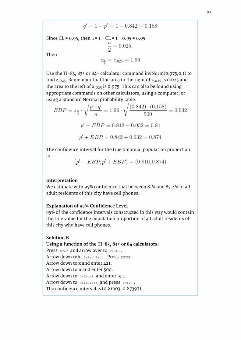
Since CL = 0.95, then α = 1 − CL = 1 − 0.95 = 0.05

Then

Use the TI-83, 83+ or 84+ calculator command invNorm(0.975,0,1) tofind z.025. Remember that the area to the right of z.025 is 0.025 and

the area to the left of x.025 is 0.975. This can also be found using

appropriate commands on other calculators, using a computer, orusing a Standard Normal probability table.

The confidence interval for the true binomial population proportionis

InterpretationWe estimate with 95% confidence that between 81% and 87.4% of alladult residents of this city have cell phones.

Explanation of 95% Confidence Level95% of the confidence intervals constructed in this way would containthe true value for the population proportion of all adult residents ofthis city who have cell phones.

Solution BUsing a function of the TI-83, 83+ or 84 calculators:Press STAT and arrow over to TESTS .Arrow down toA :1-PropZint . Press ENTER .Arrow down to x and enter 421.Arrow down to n and enter 500.Arrow down to C-Level and enter .95.Arrow down to Calculate and press ENTER .The confidence interval is (0.81003, 0.87397).

86

Example 4.9For a class project, a political science student at a large universitywants to estimate the percent of students that are registered voters.He surveys 500 students and finds that 300 are registered voters.Compute a 90% confidence interval for the true percent of studentsthat are registered voters and interpret the confidence interval.

Solution


• The first solution is step-by-step (Solution A).• The second solution uses a function of the TI-83, 83+ or 84

calculators (Solution B).

Solution Ax = 300 and n = 500.

Use the TI-83, 83+ or 84+ calculator command invNorm(0.95,0,1) tofind z.05. Remember that the area to the right of z.05 is 0.05 and the

area to the left of z.05 is 0.95. This can also be found usingappropriate commands on other calculators, using a computer, orusing a Standard Normal probability table.

The confidence interval for the true binomial population proportionis (p' − EBP, p' + EBP) = (0.564, 0.636).

Interpretation:

• We estimate with 90% confidence that the true percent of allstudents that are registered voters is between 56.4% and 63.6%.

• Alternate Wording: We estimate with 90% confidence thatbetween 56.4% and 63.6% of ALL students are registered voters.

Explanation of 90% Confidence Level90% of all confidence intervals constructed in this way contain thetrue value for the population percent of students that are registered

87

voters.

Solution BUsing a function of the TI-83, 83+ or 84 calculators:Press STAT and arrow over to TESTS .Arrow down to A:1-PropZint . Press ENTER .Arrow down to x and enter 300.Arrow down to n and enter 500.Arrow down to C-Level and enter .90.Arrow down to Calculate and press ENTER .The confidence interval is (0.564, 0.636).

4.4.1 Calculating the Sample Size nAvailable under Creative Commons-ShareAlike 4.0 International License (http://creativecommon


If researchers desire a specific margin of error, then they can use the error boundformula to calculate the required sample size. The error bound formula for apopulation proportion is

•• Solving for n gives you an equation for the sample size.

•

Example 4.10Suppose a mobile phone company wants to determine the currentpercentage of customers aged 50+ that use text messaging on theircell phone. How many customers aged 50+ should the companysurvey in order to be 90% confident that the estimated (sample)proportion is within 3 percentage points of the true populationproportion of customers aged 50+ that use text messaging on theircell phone.

SolutionFrom the problem, we know that EBP=0.03 (3% 0.03) and

because the confidence level is 90%

However, in order to find n , we need to know the estimated (sample)proportion p'. Remember that q' = 1-p'. But, we do not know p' yet.Since we multiply p' and q' together, we make them both equal to 0.5because p'q' = (.5)(.5) = .25 results in the largest possible product.(Try other products: (.6)(.4) = .24; (.3)(.7) = .21; (.2)(.8) = .16 and soon). The largest possible product gives us the largest n. This gives us

88




a large enough sample so that we can be 90% confident that we arewithin 3 percentage points of the true population proportion. Tocalculate the sample size n, use the formula and make thesubstitutions.

Round the answer to the next higher value. The sample size should be752 cell phone customers aged 50+ in order to be 90% confident thatthe estimated (sample) proportion is within 3 percentage points ofthe true population proportion of all customers aged 50+ that use textmessaging on their cell phone.

**With contributions from Roberta Bloom.

89

Chapter 5 Hypothesis Testing

5.1 Hypothesis Testing of Single Mean and SingleProportion: Introduction




• Diferentiate between Type I and Type II Errors• Describe hypothesis testing in general and in practice• Conduct and interpret hypothesis tests for a single population mean,

population standard deviation known.• Conduct and interpret hypothesis tests for a single population mean,

population standard deviation unknown.• Conduct and interpret hypothesis tests for a single population

proportion.



One job of a statistician is to make statistical inferences about populations based onsamples taken from the population. Confidence intervals are one way to estimate apopulation parameter. Another way to make a statistical inference is to make adecision about a parameter. For instance, a car dealer advertises that its new smalltruck gets 35 miles per gallon, on the average. A tutoring service claims that itsmethod of tutoring helps 90% of its students get an A or a B. A company says thatwomen managers in their company earn an average of $60,000 per year.

A statistician will make a decision about these claims. This process iscalled "hypothesis testing." A hypothesis test involves collecting data from a sampleand evaluating the data. Then, the statistician makes a decision as to whether or notthere is sufcient evidence based upon analyses of the data, to reject the nullhypothesis.

In this chapter, you will conduct hypothesis tests on single means and singleproportions. You will also learn about the errors associated with these tests.

Hypothesis testing consists of two contradictory hypotheses or statements, a decisionbased on the data, and a conclusion. To perform a hypothesis test, a statistician will:

90







1. Set up two contradictory hypotheses.2. Collect sample data (in homework problems, the data or summary statistics will

be given to you).3. Determine the correct distribution to perform the hypothesis test.4. Analyze sample data by performing the calculations that ultimately will allow you

to reject or fail to reject the null hypothesis.5. Make a decision and write a meaningful conclusion.

Note: To do the hypothesis test homework problems for this chapter and laterchapters, make copies of the appropriate special solution sheets. See the Tableof Contents topic "Solution Sheets".

5.2 Hypothesis Testing of Single Mean and SingleProportion: Null and Alternate Hypotheses



The actual test begins by considering two hypotheses. They are called the nullhypothesis and the alternate hypothesis. These hypotheses contain opposingviewpoints.

Ho: The null hypothesis: It is a statement about the population that will be assumedto be true unless it can be shown to be incorrect beyond a reasonable doubt.

Ha: The alternate hypothesis: It is a claim about the population that is contradictoryto Ho and what we conclude when we reject Ho.

Example 5.1Ho: No more than 30% of the registered voters in Santa Clara County

voted in the primary election.

Ha: More than 30% of the registered voters in Santa Clara County

voted in the primary election.

Example 5.2We want to test whether the mean grade point average in Americancolleges is different from 2.0 (out of 4.0).

91




Example 5.3We want to test if college students take less than five years tograduate from college, on the average.

Example 5.4In an issue of U. S. News and World Report, an article on schoolstandards stated that about half of all students in France, Germany,and Israel take advanced placement exams and a third pass. Thesame article stated that 6.6% of U. S. students take advancedplacement exams and 4.4 % pass. Test if the percentage of U. S.students who take advanced placement exams is more than 6.6%.

Since the null and alternate hypotheses are contradictory, you must examine evidenceto decide if you have enough evidence to reject the null hypothesis or not. Theevidence is in the form of sample data.

After you have determined which hypothesis the sample supports, you make adecision. There are two options for a decision. They are "reject Ho" if the sampleinformation favors the alternate hypothesis or "do not reject Ho" or "fail to reject Ho"if the sample information is insufficient to reject the null hypothesis.

Mathematical Symbols Used in Ho and Ha:

Ho Ha

equal (=)not equal ( ) or greater than (>) or lessthan (<)

greater than or equalto (≥)

less than (<)

less than or equal to(≤)

more than (>)

Note: Ho always has a symbol with an equal in it. Ha never has a symbol with

an equal in it. The choice of symbol depends on the wording of the hypothesistest. However, be aware that many researchers (including one of the co-authors in research work) use = in the Null Hypothesis, even with > or < as the

92

symbol in the Alternate Hypothesis. This practice is acceptable because weonly make the decision to reject or not reject the Null Hypothesis.



Bring to class a newspaper, some news magazines, and some Internet articles . Ingroups, find articles from which your group can write a null and alternate hypotheses.Discuss your hypotheses with the rest of the class.

5.3 Hypothesis Testing of Single Mean and SingleProportion: Using the Sample to Test the NullHypothesis



Use the sample data to calculate the actual probability of getting the test result,called the p-value. The p-value is the probability that, if the null hypothesis istrue, the results from another randomly selected sample will be as extreme ormore extreme as the results obtained from the given sample.

A large p-value calculated from the data indicates that we should fail to reject the nullhypothesis. The smaller the p-value, the more unlikely the outcome, and the strongerthe evidence is against the null hypothesis. We would reject the null hypothesis if theevidence is strongly against it.

Draw a graph that shows the p-value. The hypothesis test is easier to perform ifyou use a graph because you see the problem more clearly.

Example 5.5: (to illustrate the p-value)Suppose a baker claims that his bread height is more than 15 cm, onthe average. Several of his customers do not believe him. To persuadehis customers that he is right, the baker decides to do a hypothesistest. He bakes 10 loaves of bread. The mean height of the sampleloaves is 17 cm. The baker knows from baking hundreds of loaves ofbread that the standard deviation for the height is 0.5 cm. and thedistribution of heights is normal.

The null hypothesis could be Ho: µ ≤ 15

The alternate hypothesis is Ha: µ> 15

The words "is more than" translates as a ">" so "µ> 15" goes intothe alternate hypothesis. The null hypothesis must contradict thealternate hypothesis.

93







Since σ is known (σ =0.5 cm.), the distribution for the population isknown to be normal with mean µ= 15 and standard deviation

Suppose the null hypothesis is true (the mean height of the loaves isno more than 15 cm). Then is the mean height (17 cm) calculatedfrom the sample unexpectedly large? The hypothesis test works byasking the question how unlikely the sample mean would be if thenull hypothesis were true. The graph shows how far out the samplemean is on the normal curve. The p-value is the probability that, ifwe were to take other samples, any other sample mean would fall atleast as far out as 17 cm.

The p-value, then, is the probability that a sample mean is thesame or greater than 17 cm. when the population mean is, in fact,15 cm. We can calculate this probability using the normal distributionfor means from Chapter 7.

p-value = P ( > 17) which is approximately 0.

A p-value of approximately 0 tells us that it is highly unlikely that aloaf of bread rises no more than 15 cm, on the average. That is, almost0% of all loaves of bread would be at least as high as 17 cm. purely byCHANCE had the population mean height really been 15 cm. Becausethe outcome of 17 cm. is so unlikely (meaning it is happening NOTby chance alone), we conclude that the evidence is strongly againstthe null hypothesis (the mean height is at most 15 cm.). There issufcient evidence that the true mean height for the population of thebaker's loaves of bread is greater than 15 cm.

94

5.4 Hypothesis Testing of Single Mean and SingleProportion: Decision and Conclusion



A systematic way to make a decision of whether to reject or not reject the nullhypothesis is to compare the p-value and a preset or preconceived α (also called a"significance level"). A preset α is the probability of a Type I error (rejecting the nullhypothesis when the null hypothesis is true). It may or may not be given to you at thebeginning of the problem.

When you make a decision to reject or not reject Ho, do as follows:

• If α > p-value, reject Ho. The results of the sample data are significant. There issufficient evidence to conclude that Ho is an incorrect belief and that thealternative hypothesis, Ha, may be correct.

• If α ≤ p-value, do not reject Ho. The results of the sample data are not significant.There is not sufficient evidence to conclude that the alternative hypothesis, Ha,may be correct.

• When you "do not reject Ho", it does not mean that you should believe that Ho istrue. It simply means that the sample data have failed to provide sufficientevidence to cast serious doubt about the truthfulness of Ho.

Conclusion: After you make your decision, write a thoughtful conclusion about thehypotheses in terms of the given problem.

95




Chapter 6 Linear Regression andCorrelation

6.1 Linear Regression and Correlation: Introduction




• Discuss basic ideas of linear regression and correlation.• Create and interpret a line of best fit.• Calculate and interpret the correlation coefficient.• Calculate and interpret outliers.



Professionals often want to know how two or more numeric variables are related. Forexample, is there a relationship between the grade on the second math exam astudent takes and the grade on the final exam? If there is a relationship, what is it andhow strong is the relationship?

In another example, your income may be determined by your education, yourprofession, your years of experience, and your ability. The amount you pay a repairperson for labor is often determined by an initial amount plus an hourly fee. These areall examples in which regression can be used.

The type of data described in the examples is bivariate data -"bi" for two variables. Inreality, statisticians use multivariate data, meaning many variables.

In this chapter, you will be studying the simplest form of regression, "linearregression" with one independent variable (x). This involves data that fits a line in twodimensions. You will also study correlation which measures how strong therelationship is.

96







6.2 Linear Regression and Correlation: Linear EquationsAvailable under Creative Commons-ShareAlike 4.0 International License (http://creativecommon


Linear regression for two variables is based on a linear equation with oneindependent variable. It has the form:

where a and b are constant numbers.

x is the independent variable, and y is the dependent variable. Typically, youchoose a value to substitute for the independent variable and then solve for thedependent variable.

Example 6.1The following examples are linear equations.

The graph of a linear equation of the form y = a + bx is a straight line.Any line that is not vertical can be described by this equation.

Example 6.2:

Figure 6.1 Graph of the equation y = −1+ 2x.

Linear equations of this form occur in applications of life sciences,social sciences, psychology, business, economics, physical sciences,mathematics, and other areas.

97




Example 6.3Aaron's Word Processing Service (AWPS) does word processing. Itsrate is $32 per hour plus a $31.50 one-time charge. The total cost to acustomer depends on the number of hours it takes to do the wordprocessing job.


ProblemFind the equation that expresses the total cost in terms of thenumber of hours required to finish the word processing job.

SolutionLet x = the number of hours it takes to get the job done.Let y = the total cost to the customer.

The $31.50 is a fixed cost. If it takes x hours to complete the job, then(32) (x) is the cost of the word processing only. The total cost is:

6.3 Linear Regression and Correlation: Slope and Y-Intercept of a Linear Equation



For the linear equation y = a + bx, b = slope and a = y-intercept.

From algebra recall that the slope is a number that describes the steepness of a lineand the y-intercept is the y coordinate of the point (0,a) where the line crosses the y-axis.

Figure 6.2 Three possible graphs of y = a + bx. (a) If b> 0, the line slopes upward to the right. (b) If b

=0, the line is horizontal. (c) If b< 0, the line slopes downward to the right.

98




Example 6.4Svetlana tutors to make extra money for college. For each tutoringsession, she charges a one time fee of $25 plus $15 per hour oftutoring. A linear equation that expresses the total amount of moneySvetlana earns for each session she tutors is y = 25+ 15x.


ProblemWhat are the independent and dependent variables? What is the y-intercept and what is the slope? Interpret them using completesentences.

SolutionThe independent variable (x) is the number of hours Svetlana tutorseach session. The dependent variable (y) is the amount, in dollars,Svetlana earns for each session.

The y-intercept is 25 (a = 25). At the start of the tutoring session,Svetlana charges a one-time fee of $25 (this is when x = 0). The slopeis 15 (b = 15). For each session, Svetlana earns $15 for each hour shetutors.

6.4 Linear Regression and Correlation: Scatter PlotsAvailable under Creative Commons-ShareAlike 4.0 International License (http://creativecommon


Before we take up the discussion of linear regression and correlation, we need toexamine a way to display the relation between two variables x and y. The mostcommon and easiest way is a scatter plot. The following example illustrates a scatterplot.

Example 6.5From an article in the Wall Street Journal: In Europe and Asia, m-commerce is popular. M-commerce users have special mobile phonesthat work like electronic wallets as well as provide phone andInternet services. Users can do everything from paying for parking tobuying a TV set or soda from a machine to banking to checking sportsscores on the Internet. For the years 2000 through 2004, was there arelationship between the year and the number of m-commerceusers? Construct a scatter plot. Let x = the year and let y = the numberof m-commerce users, in millions.

99




x (year) y (# of users)

2000 0.5

2002 20.0

2003 33.0

2004 47.0

Table 6.1 Table showing the number of m-commerce users(in millions) by year.

Figure 6.3 Scatter plot showing the number of m-commerce users (in millions) by year.

A scatter plot shows the direction and strength of a relationship between thevariables. A clear direction happens when there is either:

• High values of one variable occurring with high values of the other variable or lowvalues of one variable occurring with low values of the other variable.

• High values of one variable occurring with low values of the other variable.

You can determine the strength of the relationship by looking at the scatter plot andseeing how close the points are to a line, a power function, an exponential function, orto some other type of function.

When you look at a scatterplot, you want to notice the overall pattern and anydeviations from the pattern. The following scatterplot examples illustrate theseconcepts.

100

Figure 6.4 (a) Positive Linear Pattern (Strong) (b) Linear Pattern w/ One Deviation

Figure 6.5 (a) Negative Linear Pattern (Strong) (b) Negative Linear Pattern (Weak)

Figure 6.6 (a) Exponential Growth Pattern (b) No Pattern

In this chapter, we are interested in scatter plots that show a linear pattern. Linearpatterns are quite common. The linear relationship is strong if the points are close toa straight line. If we think that the points show a linear relationship, we would like todraw a line on the scatter plot. This line can be calculated through a process calledlinear regression. However, we only calculate a regression line if one of the variableshelps to explain or predict the other variable. If x is the independent variable and y thedependent variable, then we can use a regression line to predict y for a given value ofx.

6.5 Linear Regression and Correlation: The RegressionEquation



Data rarely fit a straight line exactly. Usually, you must be satisfied with roughpredictions. Typically, you have a set of data whose scatter plot appears to "fit" astraight line. This is called a Line of Best Fit or Least Squares Line.

101






If you know a person's pinky (smallest) finger length, do you think you could predictthat person's height? Collect data from your class (pinky finger length, in inches). Theindependent variable, x, is pinky finger length and the dependent variable, y, is height.

For each set of data, plot the points on graph paper. Make your graph big enough anduse a ruler. Then "by eye" draw a line that appears to "fit" the data. For your line, picktwo convenient points and use them to find the slope of the line. Find the y-interceptof the line by extending your lines so they cross the y-axis. Using the slopes and the y-intercepts, write your equation of "best fit". Do you think everyone will have the sameequation? Why or why not?

Using your equation, what is the predicted height for a pinky length of 2.5 inches?

Example 6.6A random sample of 11 statistics students produced the followingdata where x is the third exam score, out of 80, and y is the final examscore, out of 200. Can you predict the final exam score of a randomstudent if you know the third exam score?

x (third exam score) y (fnal exam score)

65 175

67 133

71 185

71 163

66 126

75 198

67 153

70 163

Table 6.2 Table showing the scores on the final exam basedon scores from the third exam.

102




x (third exam score) y (fnal exam score)

71 159

69 151

69 159

Table 6.2 Table showing the scores on the final exam basedon scores from the third exam.

Figure 6.7 Scatter plot showing the scores on the fnal exam based on scores from the third exam.

The third exam score, x, is the independent variable and the final exam score, y, is thedependent variable. We will plot a regression line that best "fits" the data. If each ofyou were to fit a line "by eye", you would draw different lines. We can use what iscalled a least-squares regression line to obtain the best fit line. Consider thefollowing diagram. Each point of data is of the form (x, y) and each point of the line ofbest fit using least-squares linear regression has the form (x, ).

The is read "y hat" and is the estimated value of y. It is the value of y obtainedusing the regression line. It is not generally equal to y from data.

103

Figure 6.8

The term

is called the "error" or residual. It is not an error in the sense of a mistake.The absolute value of a residual measures the vertical distance between the actualvalue of y and the estimated value of y. In other words, it measures the verticaldistance between the actual data point and the predicted point on the line.

If the observed data point lies above the line, the residual is positive, and the lineunderestimates the actual data value for y. If the observed data point lies below theline, the residual is negative, and the line overestimates that actual data value for y.

In the diagram above, is the residual for the point shown. Here thepoint lies above the line and the residual is positive.

= the Greek letter epsilon

For each data point, you can calculate the residuals or errors,

Each is a vertical distance.

For the example about the third exam scores and the fnal exam scores for the 11statistics students, there are 11 data points. Therefore, there are 11 values. If yousquare each and add, you get

This is called the Sum of Squared Errors (SSE).

Using calculus, you can determine the values of a and b that make the SSE aminimum. When you make the SSE a minimum, you have determined the points thatare on the line of best fit. It turns out that the line of best fit has the equation:

where

104

and

and are the sample means of the x values and the y values, respectively. The bestfit line always passes through the point ( , ).

The slope b can be written as

where sy = the standard deviation of the y values and sx the standard deviation of thex values. r is the correlation coefficient which is discussed in the next section.

Least Squares Criteria for Best Fit

The process of fitting the best fit line is called linear regression. The idea behindfinding the best fit line is based on the assumption that the data are scattered about astraight line. The criteria for the best fit line is that the sum of the squared errors (SSE)is minimized, that is made as small as possible. Any other line you might choose wouldhave a higher SSE than the best fit line. This best fit line is called the least squaresregression line.

Note: Computer spreadsheets, statistical software, and many calculators canquickly calculate the best fit line and create the graphs. The calculations tendto be tedious if done by hand. Instructions to use the TI-83, TI-83+, and TI-84+calculators to find the best fit line and create a scatterplot are shown at the endof this section.

THIRD EXAM vs FINAL EXAM EXAMPLE:

The graph of the line of best fit for the third exam/final exam example is shown below:

Figure 6.9 Exam Score

The least squares regression line (best fit line) for the third exam/final exam examplehas the equation:

105

Note: Remember, it is always important to plot a scatter diagram first. If thescatter plot indicates that there is a linear relationship between the variables,then it is reasonable to use a best fit line to make predictions for y given xwithin the domain of x-values in the sample data, but not necessarily for x-values outside that domain.

Remember, it is always important to plot a scatter diagram first. If the scatter plotindicates that there is a linear relationship between the variables, then it is reasonableto use a best fit line to make predictions for y given x within the domain of x-values inthe sample data, but not necessarily for x-values outside that domain.

You could use the line to predict the final exam score for a student who earned agrade of 73 on the third exam.

You should NOT use the line to predict the final exam score for a student who earneda grade of 50 on the third exam, because 50 is not within the domain of the x-values inthe sample data, which are between 65 and 75.

UNDERSTANDING SLOPE

The slope of the line, b, describes how changes in the variables are related. It isimportant to interpret the slope of the line in the context of the situation representedby the data. You should be able to write a sentence interpreting the slope in plainEnglish.

INTERPRETATION OF THE SLOPE: The slope of the best fit line tells us how thedependent variable (y) changes for every one unit increase in the independent (x)variable, on average.

THIRD EXAM vs FINAL EXAM EXAMPLE

Slope: The slope of the line is b 4.83.Interpretation: For a one point increase in the score on the third exam, the fnal examscore increases by 4.83 points, on average.

6.5.2 Using the TI-83+ and TI-84+ CalculatorsAvailable under Creative Commons-ShareAlike 4.0 International License (http://creativecommon


Using the Linear Regression T Test: LinRegTTest

Step 1. In the STAT list editor, enter the X data in list L1 and the Y data in list L2, pairedso that the corresponding (x,y) values are next to each other in the lists. (If a particularpair of values is repeated, enter it as many times as it appears in the data.)

Step 2. On the STAT TESTS menu, scroll down with the cursor to select theLinRegTTest. (Be careful to select LinRegTTest as some calculators may also have adifferent item called LinRegTInt.)

Step 3. On the LinRegTTest input screen enter: Xlist: L1 ; Ylist: L2 ; Freq: 1

Step 4. On the next line, at the prompt β or ρ, highlight " 0" and press ENTER

106




Step 5. Leave the line for "RegEq:" blank Step 6. Highlight Calculate and press ENTER.

Figure 6.10 LinRegTTest Screen

The output screen contains a lot of information. For now we will focus on a few itemsfrom the output, and will return later to the other items.

The second line says y = a + bx. Scroll down to find the values a = -173.513, and b =4.8273 ; the equation of

the best fit line is

The two items at the bottom are r2 = .43969 and r =.663. For now, just note where tofind these values; we will discuss them in the next two sections.

Graphing the Scatterplot and Regression Line

Step 1. We are assuming your X data is already entered in list L1 and your Y data is inlist L2

Step 2. Press 2nd STATPLOT ENTER to use Plot 1

Step 3. On the input screen for PLOT 1, highlight On and press ENTER

Step 4. For TYPE: highlight the very first icon which is the scatterplot and press ENTER

Step 5. Indicate Xlist: L1 and Ylist: L2

Step 6. For Mark: it does not matter which symbol you highlight.

Step 7. Press the ZOOM key and then the number 9 (for menu item "ZoomStat") ; thecalculator will ft the window to the data

Step 8. To graph the best ft line, press the "Y " key and type the equation -173.5+4.83Xinto equation Y1. (The X key is immediately left of the STAT key). Press ZOOM 9 againto graph it.

Step 9. Optional: If you want to change the viewing window, press the WINDOW key.Enter your desired window using Xmin, Xmax, Ymin, Ymax

107


6.6 Linear Regression and Correlation: CorrelationCoefficient and Coefficient of Determination

6.6.1 The Correlation Coefficient rAvailable under Creative Commons-ShareAlike 4.0 International License (http://creativecommon


Besides looking at the scatter plot and seeing that a line seems reasonable, how canyou tell if the line is a good predictor? Use the correlation coefficient as anotherindicator (besides the scatterplot) of the strength of the relationship between x and y.

The correlation coefficient, r, developed by Karl Pearson in the early 1900s, is anumerical measure of the strength of association between the independent variable xand the dependent variable y.The correlation coefficient is calculated as

where n = the number of data points.

If you suspect a linear relationship between x and y, then r can measure how strongthe linear relationship is.

What the VALUE of r tells us:

• The value of r is always between -1 and +1: −1 ≤ r ≤ 1.• The size of the correlation r indicates the strength of the linear relationship

between x and y. Values of r close to -1 or to +1 indicate a stronger linearrelationship between x and y.

• If r = 0 there is absolutely no linear relationship between x and y (no linearcorrelation).

• If r = 1, there is perfect positive correlation. If r = −1, there is perfect negativecorrelation. In both these cases, all of the original data points lie on a straight line.Of course, in the real world, this will not generally happen.

What the SIGN of r tells us

• A positive value of r means that when x increases, y tends to increase and when xdecreases, y tends to decrease (positive correlation).

• A negative value of r means that when x increases, y tends to decrease and whenx decreases, y tends to increase (negative correlation).

• The sign of r is the same as the sign of the slope, b, of the best fit line.

Note: Strong correlation does not suggest that x causes y or y causes x. We say"correlation does not imply causation." For example, every person wholearned math in the 17th century is dead. However, learning math does notnecessarily cause death!

108




Figure 6.11 (a) A scatter plot showing data with a positive correlation. 0 <r< 1 (b) A scatter plot

showing data with a negative correlation. −1 <r< 0

Figure 6.12 (C) A scatter plot showing data with zero correlation. r=0

The formula for r looks formidable. However, computer spreadsheets, statisticalsoftware, and many calculators can quickly calculate r. The correlation coefficient r isthe bottom item in the output screens for the LinRegTTest on the TI-83, TI-83+, orTI-84+ calculator (see previous section for instructions).

6.6.2 The Coefficient of DeterminationAvailable under Creative Commons-ShareAlike 4.0 International License (http://creativecommon


r2 is called the coefficient of determination. r2 is the square of the correlation

coefficient, but is usually stated as a percent, rather than in decimal form. r2 has aninterpretation in the context of the data:

• r2, when expressed as a percent, represents the percent of variation in thedependent variable y that can be explained by variation in the independentvariable x using the regression (best fit) line.

• 1-r2, when expressed as a percent, represents the percent of variation in y that isNOT explained by variation in x using the regression line. This can be seen as thescattering of the observed data points about the regression line.

Consider the third exam/final exam example introduced in the previous section

The line of best fit is:

The correlation coefficient is r = 0.6631

The coefficient of determination is r2 = 0.66312 = 0.4397

109




Interpretation of r2 in the context of this example:

Approximately 44% of the variation (0.4397 is approximately 0.44) in the final examgrades can be explained by the variation in the grades on the third exam, using thebest fit regression line.

Therefore approximately 56% of the variation (1 - 0.44 = 0.56) in the fnal exam gradescan NOT be explained by the variation in the grades on the third exam, using the bestfit regression line. (This is seen as the scattering of the points about the line.)

**With contributions from Roberta Bloom.

6.7 Linear Regression and Correlation: Testing theSignificance of the Correlation Coefficient

6.7.1 Testing the Significance of the Correlation CoefficientAvailable under Creative Commons-ShareAlike 4.0 International License (http://creativecommon


The correlation coefficient, r, tells us about the strength of the linear relationshipbetween x and y. However, the reliability of the linear model also depends on howmany observed data points are in the sample. We need to look at both the value ofthe correlation coefficient r and the sample size n, together.

We perform a hypothesis test of the "significance of the correlation coefficient" todecide whether the linear relationship in the sample data is strong enough to use tomodel the relationship in the population.

The sample data is used to computer r, the correlation coefficient for the sample. If wehad data for the entire population, we could find the population correlationcoefficient. But because we only have sample data, we can not calculate thepopulation correlation coefficient. The sample correlation coefficient, r, is our estimateof the unknown population correlation coefficient.

The symbol for the population correlation coefficient is ρ, the Greek letter "rho".

ρ = population correlation coefficient (unknown)

r = sample correlation coefficient (known; calculated from sample data)

The hypothesis test lets us decide whether the value of the population correlationcoefficient ρ is "close to 0" or "significantly different from 0". We decide this based onthe sample correlation coefficient r and the sample size n.

If the test concludes that the correlation coefficient is significantly differentfrom 0, we say that the correlation coefficient is "significant".

• Conclusion: "There is sufficient evidence to conclude that there is a significantlinear relationship between x and y because the correlation coefficient issignificantly different from 0."

110




• What the conclusion means: There is a significant linear relationship between xand y. We can use the regression line to model the linear relationship between xand y in the population.

If the test concludes that the correlation coefficient is not significantly differentfrom 0 (it is close to 0), we say that correlation coefficient is "not significant".

• Conclusion: "There is insufficient evidence to conclude that there is a significantlinear relationship between x and y because the correlation coefficient is notsignificantly different from 0."

• What the conclusion means: There is not a significant linear relationship betweenx and y. Therefore we can NOT use the regression line to model a linearrelationship between x and y in the population.

Note:• If r is significant and the scatter plot shows a linear trend, the line can be used to

predict the value of y for values of x that are within the domain of observed xvalues.

• If r is not significant OR if the scatter plot does not show a linear trend, the lineshould not be used for prediction.

• If r is significant and if the scatter plot shows a linear trend, the line may NOT beappropriate or reliable for prediction OUTSIDE the domain of observed x valuesin the data.

PERFORMING THE HYPOTHESIS TESTSETTING UP THE HYPOTHESES:

• Null Hypothesis:

• Alternate Hypothesis:

What the hypotheses mean in words:

• Null Hypothesis Ho: The population correlation coefficient IS NOT significantlydifferent from 0. There IS NOT a significant linear relationship(correlation)between x and y in the population.

• Alternate Hypothesis Ha: The population correlation coefficient IS significantlyDIFFERENT FROM 0. There IS A SIGNIFICANT LINEAR RELATIONSHIP (correlation)between x and y in the population.

DRAWING A CONCLUSION:

There are two methods to make the decision. Both methods are equivalent and givethe same result.

Method 1: Using the p-value

Method 2: Using a table of critical values

In this chapter of this textbook, we will always use a significance level of 5%, α = 0.05

Note: Using the p-value method, you could choose any appropriatesignificance level you want; you are not limited to using α = 0.05. But the table

111

of critical values provided in this textbook assumes that we are using asignificance level of 5%, α = 0.05. (If we wanted to use a different significancelevel than 5% with the critical value method, we would need different tables ofcritical values that are not provided in this textbook.)

METHOD 1: Using a p-value to make a decision

The linear regression t-test LinRegTTEST on the TI-83+ or TI-84+ calculators calculatesthe p-value.

On the LinRegTTEST input screen, on the line prompt for β or ρ, highlight " 0"The output screen shows the p-value on the line that reads "p = ".(Most computer statistical software can calculate the p-value.)

If the p-value is less than the significance level (α = 0.05):

• Decision: REJECT the null hypothesis.• Conclusion: "There is sufficient evidence to conclude that there is a significant

linear relationship between x and y because the correlation coefficient issignificantly different from 0."

If the p-value is NOT less than the significance level (α = 0.05):

• Decision: DO NOT REJECT the null hypothesis.• Conclusion: "There is insufficient evidence to conclude that there is a significant

linear relationship between x and y because the correlation coefficient is NOTsignificantly different from 0."

Calculation Notes:

You will use technology to calculate the p-value. The following describe thecalculations to compute the test statistics and the p-value:The p-value is calculated using a t-distribution with n − 2 degrees of freedom.

The formula for the test statistic is . The value of the test statistic, t, isshown in the computer or calculator output along with the p-value. The test statistic thas the same sign as the correlation coefficient r.

The p-value is the combined area in both tails.

An alternative way to calculate the p-value (p) given by LinRegTTest is the command2*tcdf(abs(t),10^99, n-2) in 2nd DISTR.

THIRD EXAM vs FINAL EXAM EXAMPLE: p value method

• Consider the third exam/final exam example.• The line of best fit is: with r =0.6631 and there are n = 11

data points.• Can the regression line be used for prediction? Given a third exam score (x

value), can we use the line to predict the final exam score (predicted yvalue)?

112

The p-value is 0.026 (from LinRegTTest on your calculator or from computer software)The p-value, 0.026, is less than the signifcance level of α = 0.05Decision: Reject the Null Hypothesis Ho

Conclusion: There is sufcient evidence to conclude that there is a significant linearrelationship between x and y because the correlation coefficient is significantlydifferent from 0.

Because r is significant and the scatter plot shows a linear trend, the regressionline can be used to predict final exam scores.

METHOD 2: Using a table of Critical Values to make a decision

The 95% Critical Values of the Sample Correlation Coefficient Table at the end ofthis chapter (before the Summary) may be used to give you a good idea of whetherthe computed value of r is significant or not. Compare r to the appropriate criticalvalue in the table. If r is not between the positive and negative critical values, then thecorrelation coefficient is significant. If r is significant, then you may want to use the linefor prediction.

Example 6.7Suppose you computed r =0.801 using n = 10 data points. df = n − 2 =10 − 2= 8. The critical values associated with df = 8 are -0.632 and +0.632. If r< negative critical value or r> positive critical value, then r issignificant. Since r = 0.801 and 0.801 > 0.632, r is significant and theline may be used for prediction. If you view this example on a numberline, it will help you.

Figure 6.13 r is not significant between -0.632 and +0.632. r = 0.801 > +0.632.

Therefore, r is significant.

Example 6.8Suppose you computed r = −0.624 with 14 data points. df = 14 − 2 = 12.The critical values are -0.532 and 0.532. Since −0.624<−0.532, r issignificant and the line may be used for prediction

Figure 6.14 r = −0.624<−0.532. Therefore, r is significant.

113

Example 6.9Suppose you computed r = 0.776 and n = 6. df = 6 − 2= 4. The criticalvalues are -0.811 and 0.811. Since −0.811 < 0.776 < 0.811, r is notsignificant and the line should not be used for prediction.

Figure 6.15 −0.811<r =0.776<0.811. Therefore, r is not significant.

THIRD EXAM vs FINAL EXAM EXAMPLE: critical value method

• Consider the third exam final exam example.• The line of best fit is: with r = 0.6631 and there are n =

11 data points.• Can the regression line be used for prediction? Given a third exam score (x

value), can we use the line to predict the final exam score (predicted yvalue)?

Use the "95% Critical Value" table for r with df = n − 2 = 11 − 2 = 9

The critical values are -0.602 and +0.602

Since 0.6631 > 0.602, r is significant.

Decision: Reject Ho:

Conclusion: There is sufficient evidence to conclude that there is a significant linearrelationship between x and y because the correlation coefficient is significantlydifferent from 0.

Because r is significant and the scatter plot shows a linear trend, the regressionline can be used to predict final exam scores.

Example 6.10: Additional PracticeExamples using Critical Values

Suppose you computed the following correlation coefficients. Usingthe table at the end of the chapter, determine if r is significant andthe line of best fit associated with each r can be used to predict a yvalue. If it helps, draw a number line.

1. r = −0.567 and the sample size, n, is 19. The df = n − 2 = 17. Thecritical value is -0.456. −0.567<−0.456 so r is significant.

2. r = 0.708 and the sample size, n, is 9. The df = n − 2 = 7. The criticalvalue is 0.666.

3. 0.708 > 0.666 so r is significant.

114

4. r = 0.134 and the sample size, n, is 14. The df = 14 − 2 = 12. Thecritical value is 0.532.

5. 0.134 is between -0.532 and 0.532 so r is not significant.6. r = 0 and the sample size, n, is 5. No matter what the dfs are, r = 0

is between the two critical values so r is not significant.

6.7.2 Assumptions in Testing the Significance of theCorrelation Coefficient



Testing the significance of the correlation coefficient requires that certain assumptionsabout the data are satisfied. The premise of this test is that the data are a sample ofobserved points taken from a larger population. We have not examined the entirepopulation because it is not possible or feasible to do so. We are examining thesample to draw a conclusion about whether the linear relationship that we seebetween x and y in the sample data provides strong enough evidence so that we canconclude that there is a linear relationship between x and y in the population.

The regression line equation that we calculate from the sample data gives the best fitline for our particular sample. We want to use this best fit line for the sample as anestimate of the best fit line for the population. Examining the scatterplot and testingthe significance of the correlation coefficient helps us determine if it is appropriate todo this.

The assumptions underlying the test of significance are:

• There is a linear relationship in the population that models the average value of yfor varying values of x. In other words, the expected value of y for each particularvalue lies on a straight line in the population. (We do not know the equation forthe line for the population. Our regression line from the sample is our bestestimate of this line in the population.)

• The y values for any particular x value are normally distributed about the line.This implies that there are more y values scattered closer to the line than arescattered farther away. Assumption (1) above implies that these normaldistributions are centered on the line: the means of these normal distributions ofy values lie on the line.

• The standard deviations of the population y values about the line are equal foreach value of x. In other words, each of these normal distributions of y values hasthe same shape and spread about the line.

• The residual errors are mutually independent (no pattern).

115




Figure 6.16 The y values for each x value are normally distributed about the line with the same

standard deviation. For each x value, the mean of the y values lies on the regression line. More y

values lie near the line than are scattered further away from the line.


6.8 Linear Regression and Correlation: PredictionAvailable under Creative Commons-ShareAlike 4.0 International License (http://creativecommon


Recall the third exam/final exam example.

We examined the scatterplot and showed that the correlation coefficient is significant.We found the equation of the best fit line for the final exam grade as a function of thegrade on the third exam. We can now use the least squares regression line forprediction.

Suppose you want to estimate, or predict, the final exam score of statistics studentswho received 73 on the third exam. The exam scores (x-values) range from 65 to 75.Since 73 is between the x-values 65 and 75, substitute x = 73 into the equation.Then:

We predict that statistic students who earn a grade of 73 on the third exam will earn agrade of 179.08 on the final exam, on average.

Example 6.11Recall the third exam/final exam example.

See Problem 1 - 2.

116




Problem 1What would you predict the final exam score to be for a student whoscored a 66 on the third exam?

Solution145.27

Problem 2What would you predict the final exam score to be for a student whoscored a 90 on the third exam?





The x values in the data are between 65 and 75. 90 is outside of the domain of theobserved x values in the data (independent variable), so you cannot reliably predictthe final exam score for this student. (Even though it is possible to enter x into theequation and calculate a y value, you should not do so!)

To really understand how unreliable the prediction can be outside of the observed xvalues in the data, make the substitution x = 90 into the equation.

The final exam score is predicted to be 261.19. The largest the final exam score can beis 200.

Note: The process of predicting inside of the observed x values in the data iscalled interpolation. The process of predicting outside of the observed x valuesin the data is called extrapolation.

117




Chapter 7 GlossaryAvailable under Creative Commons-ShareAlike 4.0 International License (http://creativecommon


A

Average

A number that describes the central tendency of the data. There are a number ofspecialized averages, including the arithmetic mean, weighted mean, median, mode,and geometric mean.

B

Binomial Distribution

A discrete random variable (RV) which arises from Bernoulli trials. There are a fixednumber, n, of independent trials. "Independent" means that the result of any trial (forexample, trial 1) does not affect the results of the following trials, and all trials areconducted under the same conditions. Under these circumstances the binomial RV Xis defined as the number of successes in n trials. The notation is: X∼∼B (n, p). Themean is µ = np and the standard deviation is The probability of exactly xsuccesses in n trials is

C

Central Limit Theorem

Given a random variable (RV) with known mean µ and known standard deviation σ. Weare sampling with size n and we are interested in two new RVs - the sample mean, ,and the sample sum, ΣX. If the size n of the sample is sufficiently large, then

and . If the size n of the sample issufciently large, then the distribution of the sample means and the distribution of thesample sums will approximate a normal distribution regardless of the shape of thepopulation. The mean of the sample means will equal the population mean and themean of the sample sums will equal n times the population mean. The standard

deviation of the distribution of the sample means, , is called the standard error ofthe mean.

Coefficient of Correlation

A measure developed by Karl Pearson (early 1900s) that gives the strength ofassociation between the independent variable and the dependent variable. Theformula is:

118




where n is the number of data points. The coefficient cannot be more then 1 and lessthen -1. The closer the coefficient is to ±1, the stronger the evidence of a significantlinear relationship between x and y.

Confidence Interval (CI)

An interval estimate for an unknown population parameter. This depends on:

• The desired confidence level.• Information that is known about the distribution (for example, known standard

deviation).• The sample and its size.

Confidence Level (CL)

The percent expression for the probability that the confidence interval contains thetrue population parameter. For example, if the CL = 90%, then in 90 out of 100samples the interval estimate will enclose the true population parameter.

Continuous Random Variable

A random variable (RV) whose outcomes are measured.

Example: The height of trees in the forest is a continuous RV.

Cumulative Relative Frequency

The term applies to an ordered set of observations from smallest to largest. TheCumulative Relative Frequency is the sum of the relative frequencies for all values thatare less than or equal to the given value.

D

Data

A set of observations (a set of possible outcomes). Most data can be put into twogroups: qualitative (hair color, ethnic groups and other attributes of the population)and quantitative (distance traveled to college, number of children in a family, etc.).Quantitative data can be separated into two subgroups: discrete and continuous.Data is discrete if it is the result of counting (the number of students of a given ethnicgroup in a class, the number of books on a shelf, etc.). Data is continuous if it is theresult of measuring (distance traveled, weight of luggage, etc.)

Degrees of Freedom (df)

The number of objects in a sample that are free to vary.

Discrete Random Variable

A random variable (RV) whose outcomes are counted.

E

Error Bound for a Population Mean (EBM)

The margin of error. Depends on the confidence level, sample size, and known orestimated population standard deviation.

119

Error Bound for a Population Proportion(EBP)

The margin of error. Depends on the confidence level, sample size, and the estimated(from the sample) proportion of successes.

Exponential Distribution

A continuous random variable (RV) that appears when we are interested in theintervals of time between some random events, for example, the length of time

between emergency arrivals at a hospital. Notation: X~Exp (m). The mean is

and the standard deviation is . The probability density function is f(x) = me-mx ,

x ≥ 0 and the cumulative distribution function is P (X ≤ x) = 1 – e-mx.

F

Frequency

The number of times a value of the data occurs.

H

Hypothesis

A statement about the value of a population parameter. In case of two hypotheses,the statement assumed to be true is called the null hypothesis (notation H0) and thecontradictory statement is called the alternate hypothesis (notation Ha).

Hypothesis Testing

Based on sample evidence, a procedure to determine whether the hypothesis statedis a reasonable statement and cannot be rejected, or is unreasonable and should berejected.

I

Inferential Statistics

Also called statistical inference or inductive statistics. This facet of statistics deals withestimating a population parameter based on a sample statistic. For example, if 4 outof the 100 calculators sampled are defective we might infer that 4 percent of theproduction is defective.

L

Level of Significance of the Test

Probability of a Type I error (reject the null hypothesis when it is true). Notation: α. Inhypothesis testing, the Level of Significance is called the preconceived α or the presetα.

M

Mean

A number that measures the central tendency. A common name for mean is 'average.'The term 'mean' is a shortened form of 'arithmetic mean.' By definition, the mean for

120

a sample (denoted by ) is , and themean for a population (denoted by µ) is

.

Median

A number that separates ordered data into halves. Half the values are the samenumber or smaller than the median and half the values are the same number orlarger than the median. The median may or may not be part of the data.

Mode

The value that appears most frequently in a set of data.

N

Normal Distribution

A continuous random variable (RV) with pdf , where µis the mean of the distribution and σ is the standard deviation. Notation: X∼∼ N (µ, σ).If µ =0 and σ =1, the RV is called the standard normal distribution.

P

p-value

The probability that an event will happen purely by chance assuming the nullhypothesis is true. The smaller the p-value, the stronger the evidence is against thenull hypothesis.

Parameter

A numerical characteristic of the population.

Point Estimate

A single number computed from a sample and used to estimate a populationparameter.

Population

The collection, or set, of all individuals, objects, or measurements whose propertiesare being studied.

Proportion

• As a number: A proportion is the number of successes divided by the totalnumber in the sample.

• As a probability distribution: Given a binomial random variable (RV), X∼∼B (n, p),consider the ratio of the number X of successes in n Bernouli trials to the number

n of trials. This new RV is called a proportion, and if the number of

trials, n, is large enough, .

121

Q

Qualitative Data

See Data.

Quantitative Data

R

Relative Frequency

The ratio of the number of times a value of the data occurs in the set of all outcomesto the number of all outcomes.

S

Sample

A portion of the population understudy. A sample is representative if it characterizesthe population being studied.

Standard Deviation

A number that is equal to the square root of the variance and measures how far datavalues are from their mean. Notation: s for sample standard deviation and σ forpopulation standard deviation.

Standard Error of the Mean

The standard deviation of the distribution of the sample means, .

Standard Normal Distribution

A continuous random variable (RV) X-N (0, 1) .. When X follows the standard normaldistribution, it is often noted as Z-N (0, 1).

Statistic

A numerical characteristic of the sample. A statistic estimates the correspondingpopulation parameter. For example, the average number of full-time students in a7:30 a.m. class for this term (statistic) is an estimate for the average number of full-time students in any class this term (parameter).

Student's-t Distribution

Investigated and reported by William S. Gossett in 1908 and published under thepseudonym Student. The major characteristics of the random variable (RV) are:

• It is continuous and assumes any real values.• The pdf is symmetrical about its mean of zero. However, it is more spread out

and fatter at the apex than the normal distribution.• It approaches the standard normal distribution as n gets larger.• There is a "family" of t distributions: every representative of the family is

completely defined by the number of degrees of freedom which is one less thanthe number of data.

122

T

Type 1 Error

The decision is to reject the Null hypothesis when, in fact, the Null hypothesis is true.

U

Uniform Distribution

A continuous random variable (RV) that has equally likely outcomes over the domain,a < x < b. Often referred as the Rectangular distribution because the graph of the

pdf has the form of a rectangle. Notation: X~U (a, b). The mean is and the

standard deviation is The probability density function is

for or . The cumulative distribution is

.

V

Variance

Mean of the squared deviations from the mean. Square of the standard deviation. Fora set of data, a deviation can be represented as where x is a value of the dataand is the sample mean. The sample variance is equal to the sum of the squares ofthe deviations divided by the difference of the sample size and 1.

Z

z-score

The linear transformation of the form . If this transformation is applied toany normal distribution X~N (µ, σ) , the result is the standard normal distribution Z~N(0, 1). If this transformation is applied to any specific value x of the RV with mean µand standard deviation σ , the result is called the z-score of x. Z-scores allow us tocompare data that are normally distributed but scaled differently.

123

principles of business statistics - open textbooks for ... · fields of economics, business,...

Documents