PRINCIPLES OF MACROECONOMICS

Chapter 1 Welcome to Economics!

2

Chapter Outline

1.1 Three Key Economic Ideas

1.2 The Economic Problem That Every Society Must Solve

1.3 Economic Models

1.4 Microeconomics and Macroeconomics

1.5 A Preview of Important Economic Terms

Appendix Using Graphs and Formulas

3

What is this class about?

People make choices as they try to attain their goals. Choices are

necessary because we live in a world of scarcity.

Scarcity: A situation in which unlimited wants exceed the limited

resources available to fulfill those wants.

Economics is the study of the choices people make to attain their

goals, given their scarce resources.

Economists study these choices using economic models,

simplified versions of reality used to analyze real-world economic

situations.

4

Some typical “economics” questions

We will learn how to answer questions like these:

– How are the prices of goods and services determined?

– How does pollution affect the economy, and how should

government policy deal with these effects?

– Why do firms engage in international trade, and how do

government policies affect international trade?

– Why does government control the prices of some goods and

services, and what are the effects of those controls?

55

1.1 Three Key Economic Ideas

Explain these three key economic ideas: People are rational; people respond to economic

incentives; and optimal decisions are made at the margin.

We interact with one another in markets.

Market: A group of buyers and sellers of a good or service and the

institution or arrangement by which they come together to trade.

In analyzing markets, we generally assume:

1. People are rational

2. People respond to economic incentives

3. Optimal decisions are made at the margin

6

1. People Are Rational

Economists generally assume that people are rational, using all

available information to achieve their goals.

Rational consumers and firms weigh the benefits and costs of

each action and try to make the best decision possible.

Example: Apple doesn’t randomly choose the price of its

smartwatches; it chooses the price(s) that it thinks will be most

profitable.

7

2. People Respond to Economic

Incentives

As incentives change, so do the actions that people will take.

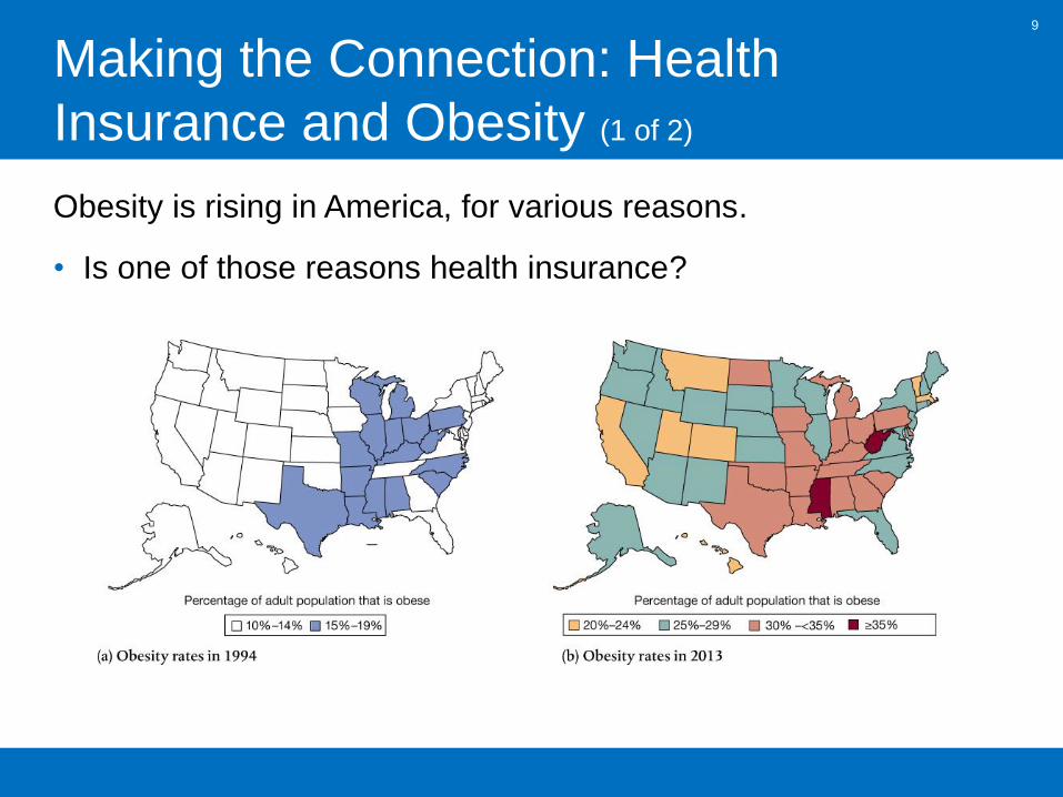
Example: Changes in several factors have resulted in increased

obesity in Americans over the last couple of decades, including:

• Decreases in the price of fast food relative to healthful food

• Improved non-active entertainment options

• Increased availability of health care and insurance, protecting

people against the consequences of their actions

8

3. Optimal Decisions Are Made at the

Margin

While some decisions are all-or-nothing, most decisions involve

doing a little more or a little less of something.

Example: Should you watch an extra hour of TV, or study instead?

Economists think about decisions like this in terms of the marginal

cost and benefit (MC and MB): the additional cost or benefit

associated with a small amount extra of some action.

Comparing MC and MB is known as marginal analysis.

9

Making the Connection: Health

Insurance and Obesity (1 of 2)

Obesity is rising in America, for various reasons.

• Is one of those reasons health insurance?

10

Making the Connection: Health

Insurance and Obesity (2 of 2)

People with health insurance have less incentive to stay healthy

than people without health insurance.

Holding constant other factors like age, gender, and income,

research shows people with health insurance are more likely to be

obese.

• They are responding to economic incentives.

1111

1.2 The Economic Problem That Every

Society Must SolveDiscuss how an economy answers these questions: What goods and services will be produced? How

will the goods and services be produced? Who will receive the goods and services produced?

In a world of scarcity, we have limited economic resources to

satisfy our desires.

• Therefore we face trade-offs.

Trade-off: The idea that, because of scarcity, producing more of

one good or service means producing less of another good or

service.

12

1. What Goods and Services Will Be

Produced?

Individuals, firms, and governments must decide on the goods and

services that should be produced.

An increase in the production of one good requires the reduction

in the production of some other good. This is a trade-off, resulting

from the scarcity of productive resources.

The highest-valued alternative given up in order to engage in

some activity is known as the opportunity cost.

Example: the opportunity cost of increased funding for space

exploration might be giving up the opportunity to fund cancer

research.

13

2. How Will the Goods and Services Be

Produced?

A firm might have several different methods for producing its

goods and services.

Example #1: A music producer can make a song sound good by

• Hiring a great singer and using standard production techniques;

• Hiring a mediocre singer and using Auto-Tune to correct the

inaccuracies.

Example #2: As the cost of manufacturing labor changes, a firm

might respond by

• Changing its production technique to one that employs more

machines and fewer workers

• Moving its factory to a location with cheaper labor

14

3. Who Will Receive the Goods and

Services Produced?

The way we are most familiar with in the United States is that

people with higher incomes obtain more goods and services.

Changes in tax and welfare policies change the distribution of

income; though people often disagree about the extent to which

this “redistribution” is desirable.

15

Types of Economies

Centrally planned economy: An economy in which the

government decides how economic resources will be allocated.

Market economy: An economy in which the decisions of

households and firms interacting in markets allocate economic

resources.

Mixed economy: An economy in which most economic decisions

result from the interaction of buyers and sellers in markets but in

which the government plays a significant role in the allocation of

resources.

16

Efficiency of Economies

Market economies tend to be more efficient than centrally-planned

economies.

Market economies promote:

• Productive efficiency, where goods or services are produced

at the lowest possible cost; and

• Allocative efficiency, where production is in accordance with

consumer preferences; in particular, every good or service is

produced up to the point where the last unit provides a marginal

benefit to society equal to the marginal cost of producing it.

17

Source of Economic Efficiency

Productive efficiency comes about because of competition.

Allocative efficiency arises due to voluntary exchange.

Voluntary exchange: A situation that occurs in markets when

both the buyer and the seller of a product are made better off by

the transaction.

• Each transaction that takes place improves the well-being of the

buyer and seller; transactions continue until no further

improvement can take place.

18

Caveats about Market Economies

Markets may not result in fully efficient outcomes. For example:

• People might not immediately do things in the most efficient way

• Governments might interfere with market outcomes

• Market outcomes might ignore the desires of people who are

not involved in transactions – ex: pollution

Economically efficient outcomes may not be the most desirable.

Markets result in high inequality; some people prefer more equity,

i.e. fairer distribution of economic benefits.

19

Market Economies and Equity

Economically efficient outcomes are not necessarily desirable.

• Less efficient outcomes may be more fair or equitable.

Equity: The fair distribution of economic benefits.

An important trade-off for a government is that between efficiency

and equity.

Example: If we tax income, people might work less or open fewer

businesses, but those tax receipts can fund programs that aid the

poor.

2020

1.3 Economic Models

Describe the role of models in economic analysis.

Economists develop economic models to analyze real-world

issues.

Building an economic model often follows these steps:

1. Decide on the assumptions to use in developing the

model.

2. Formulate a testable hypothesis.

3. Use economic data to test the hypothesis.

4. Revise the model if it fails to explain the economic data

well.

5. Retain the revised model to help answer similar economic

questions in the future.

21

Important Features of Economic Models

• Assumptions and simplifications: every model needs them in

order to be useful.

• Testability: good models generate testable predictions, which

can be verified or disproven using data.

• Economic variables: something measurable that can have

different values, such as the incomes of doctors.

22

Positive and Normative Analysis

Economists try to mimic natural scientists by using the scientific

method. But economics is a social science; studying the behavior

of people is often tricky.

When analyzing human behavior, we can perform:

• Positive analysis: analysis concerned with what is

• Normative analysis: analysis concerned with what ought to be

Economists mostly perform positive analysis.

23

Making the Connection: Should Medical

School Be Free?

Forecasts indicate a significant shortage of doctors, especially

primary care physicians, by 2020.

High costs of medical school may:

• Prevent some people from becoming doctors

• Lead people to pursue lucrative specialties instead of primary

care

Would more people become primary care physicians if medical

school were free? And if so, would it be worth the cost?

• Economic models can find answers to the positive aspects of

this debate.

2424

1.4 Microeconomics and

MacroeconomicsDistinguish between microeconomics and macroeconomics.

Microeconomics is the study of

• how households and firms make choices,

• how they interact in markets, and

• how the government attempts to influence their choices.

Macroeconomics is the study of the economy as a whole,

including topics such as inflation, unemployment, and economic

growth.

25

Table 1.1 Issues in Microeconomics and Macroeconomics

Examples of microeconomic

issues

Examples of macroeconomic

issues

• How consumers react to changes

in product prices

• How firms decide what prices to

charge for the products they sell

• Which government policy would

most efficiently reduce teenage

smoking

• What are the costs and benefits of

approving the sale of a new

prescription drug

• What is the most efficient way to

reduce air pollution

• Why economies experience

periods of recession and

increasing unemployment

• Why, over the long run, some

economies have grown much

faster than others

• What determines the inflation rate

• What determines the value of the

U.S dollar

• Whether government intervention

can reduce the severity of

recessions

2626

1.5 A Preview of Important Economic

TermsDefine important economic terms.

Like all fields of study, economics uses terms or jargon with

specific, precise meanings.

Sometimes these terms will be used in ways that differ even from

closely related disciplines.

Examples:

• Technology: the processes a firm uses to produce goods and

services

• Capital: manufactured goods that are used to produce other

goods and services

Pay close attention to terms defined in class and in the textbook!

2727

Appendix: Using Graphs and Formulas

Use graphs and formulas to analyze economic situations.

A map is a simplified

model of reality,

showing essential

details only.

Economic models, with

features like graphs and

formulas, can help us

understand economic

situations just like a map

helps us to understand

the geographic layout of

a city.

28

Figure 1A.1 Bar Graphs and Pie Charts

The left panel shows a bar graph of market share data for the U.S.

automobile industry; market share is represented by the height of the bar.

The right panel shows a pie chart of the same data; market share is

represented by the size of the “slice of the pie”.

29

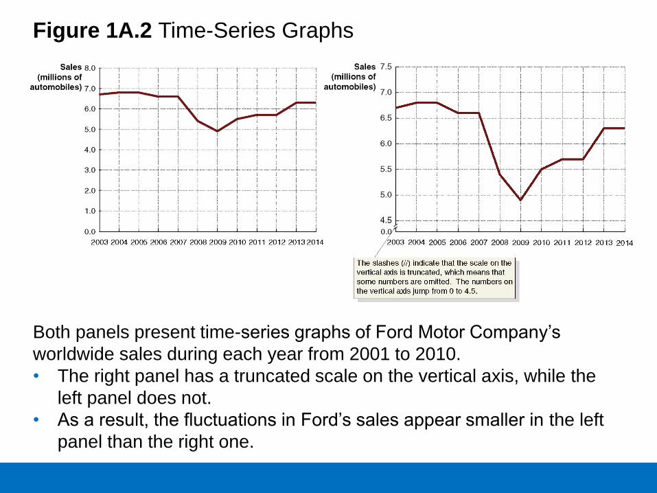
Figure 1A.2 Time-Series Graphs

Both panels present time-series graphs of Ford Motor Company’s

worldwide sales during each year from 2001 to 2010.

• The right panel has a truncated scale on the vertical axis, while the

left panel does not.

• As a result, the fluctuations in Ford’s sales appear smaller in the left

panel than the right one.

30

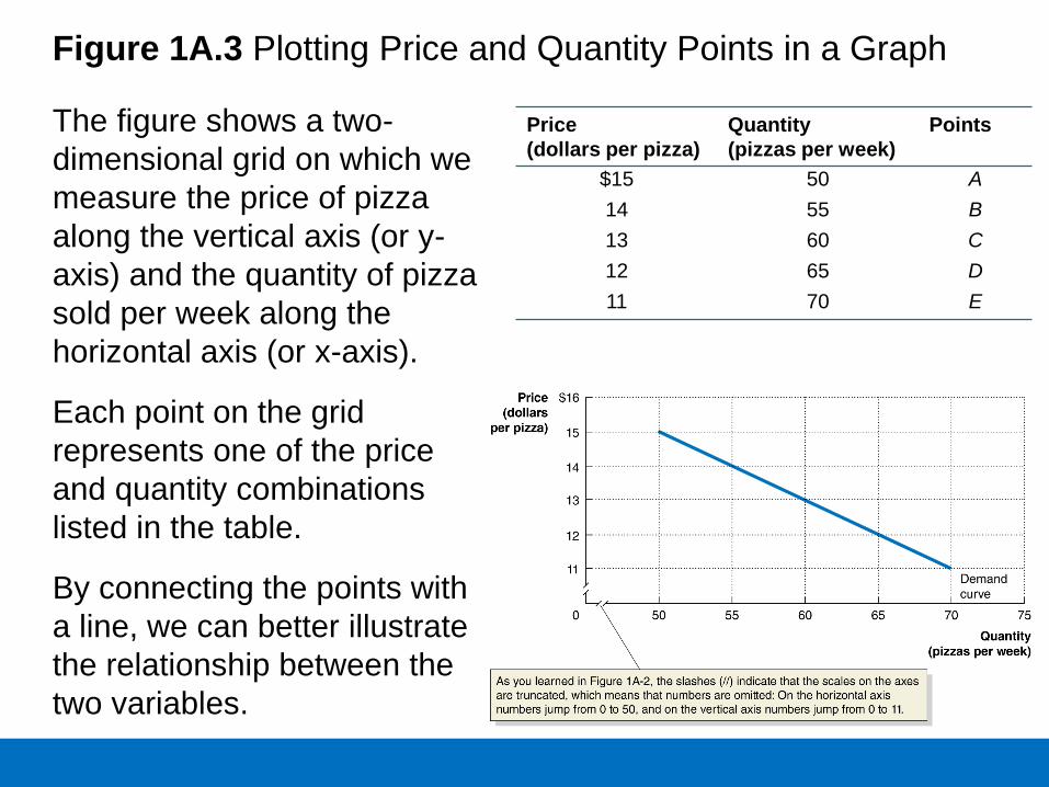
Figure 1A.3 Plotting Price and Quantity Points in a Graph

The figure shows a two-

dimensional grid on which we

measure the price of pizza

along the vertical axis (or y-

axis) and the quantity of pizza

sold per week along the

horizontal axis (or x-axis).

Each point on the grid

represents one of the price

and quantity combinations

listed in the table.

By connecting the points with

a line, we can better illustrate

the relationship between the

two variables.

Price

(dollars per pizza)

Quantity

(pizzas per week)

Points

$15 50 A

14 55 B

13 60 C

12 65 D

11 70 E

31

Figure 1A.4 Calculating the Slope of a Line (1 of 2)

We can calculate the

slope of a line as the

change in the value of

the variable on the y-axis

divided by the change in

the value of the variable

on the x-axis.

Because the slope of a

straight line is constant,

we can use any two

points in the figure to

calculate the slope of the

line.

Run

Rise

axis horizontal on the in value Change

axis verticalon the in value ChangeSlope

x

y

32

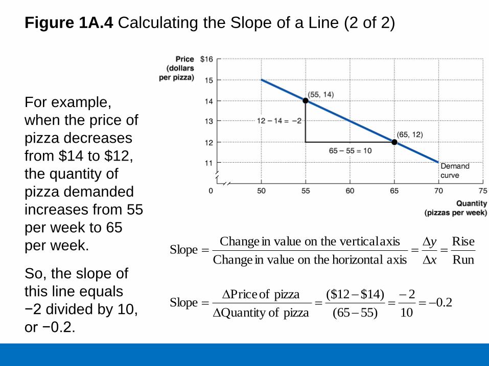
Figure 1A.4 Calculating the Slope of a Line (2 of 2)

For example,

when the price of

pizza decreases

from $14 to $12,

the quantity of

pizza demanded

increases from 55

per week to 65

per week.

So, the slope of

this line equals

−2 divided by 10,

or −0.2.

Run

Rise

axis horizontal on the in value Change

axis verticalon the in value ChangeSlope

x

y

2.010

2

)5565(

)14$12($

pizza ofQuantity

pizza of PriceSlope

33

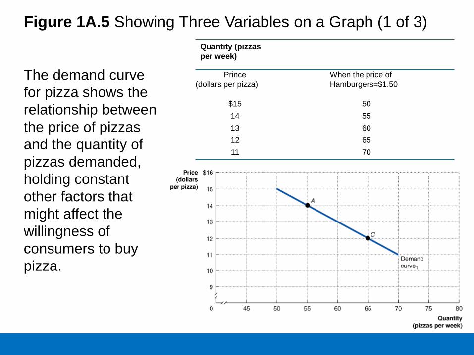
Figure 1A.5 Showing Three Variables on a Graph (1 of 3)

The demand curve

for pizza shows the

relationship between

the price of pizzas

and the quantity of

pizzas demanded,

holding constant

other factors that

might affect the

willingness of

consumers to buy

pizza.

Quantity (pizzas

per week)

Blank Blank Blank

Prince

(dollars per pizza)

Blank When the price of

Hamburgers=$1.50

Blank

$15 Blank 50 Blank

14 Blank 55 Blank

13 Blank 60 Blank

12 Blank 65 Blank

11 Blank 70 Blank

34

Figure 1A.5 Showing Three Variables on a Graph (2 of 3)

If the price of pizza

is $14 (point A), an

increase in the

price of

hamburgers from

$1.50 to $2.00

increases the

quantity of pizzas

demanded from 55

to 60 per week

(point B) and shifts

us to Demand

curve2.

Quantity

(pizzas per

week)

Blank Blank Blank

Prince

(dollars per pizza)

Blank When the price of

Hamburgers = $1.50

When the Price of

Hamburgers = $2.00

$15 Blank 50 55

14 Blank 55 60

13 Blank 60 65

12 Blank 65 70

11 Blank 70 75

35

Figure 1A.5 Showing Three Variables on a Graph (3 of 3)

Or, if we start on

Demand curve1 and

the price of pizza is

$12 (point C), a

decrease in the

price of hamburgers

from $1.50 to $1.00

decreases the

quantity of pizza

demanded from 65

to 60 per week

(point D) and shifts

us to Demand

curve3.

Quantity

(pizzas per

week)

Blank Blank Blank

Prince

(dollars per pizza)

When the Price of

Hamburgers =

$1.00

When the price of

Hamburgers = $1.50

When the Price of

Hamburgers = $2.00

$15 45 50 55

14 50 55 60

13 55 60 65

12 60 65 70

11 65 70 75

36

Figure 1A.6 Graphing the Positive Relationship between

Income and Consumption

In a positive relationship

between two economic

variables, as one variable

increases, the other

variable also increases.

In a negative relationship,

as one variable increases,

the other decreases.

This figure shows the

positive relationship

between disposable

personal income and

consumption spending.

Year

Disposable Personal

Income

(billions of dollars)

Consumption Spending

(billions of dollars)

2011 $ 11,801 $ 10,689

2012 12,384 11,083

2013 12,505 11,484

2014 12,986 11,930

37

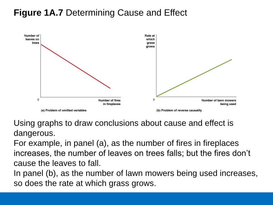
Figure 1A.7 Determining Cause and Effect

Using graphs to draw conclusions about cause and effect is

dangerous.

For example, in panel (a), as the number of fires in fireplaces

increases, the number of leaves on trees falls; but the fires don’t

cause the leaves to fall.

In panel (b), as the number of lawn mowers being used increases,

so does the rate at which grass grows.

38

Are Graphs of Economic Relationships

Always Straight Lines?

The relationship between two variables is linear when it can be

represented by a straight line.

Few economic relationships are actually linear. However linear

approximations are simpler to use and are often “good enough” in

modeling.

39

Figure 1A.8 The Slope of a Nonlinear Curve (panel (a))

A non-linear curve has different

slopes at different points. This

curve shows the total cost of

production for various quantities

of Apple Watches.

We can approximate its slope

over a section by measuring the

slope as if that section were

linear.

Between C and D, the slope is

greater than between A and B; so

we say the curve is steeper

between C and D than between A

and B.

40

Figure 1A.8 The Slope of a Nonlinear Curve (panel (b))

Another way to measure the

slope of a non-linear curve is to

measure the slope of a tangent

line to the curve, at the point we

want to know the slope.

751

75

Quantity

Cost

1501

150

Quantity

Cost

41

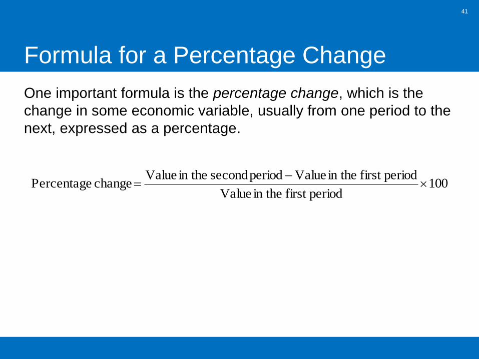
Formula for a Percentage Change

One important formula is the percentage change, which is the

change in some economic variable, usually from one period to the

next, expressed as a percentage.

100 periodfirst in the Value

periodfirst in the Valueperiod second in the Valuechange Percentage

42

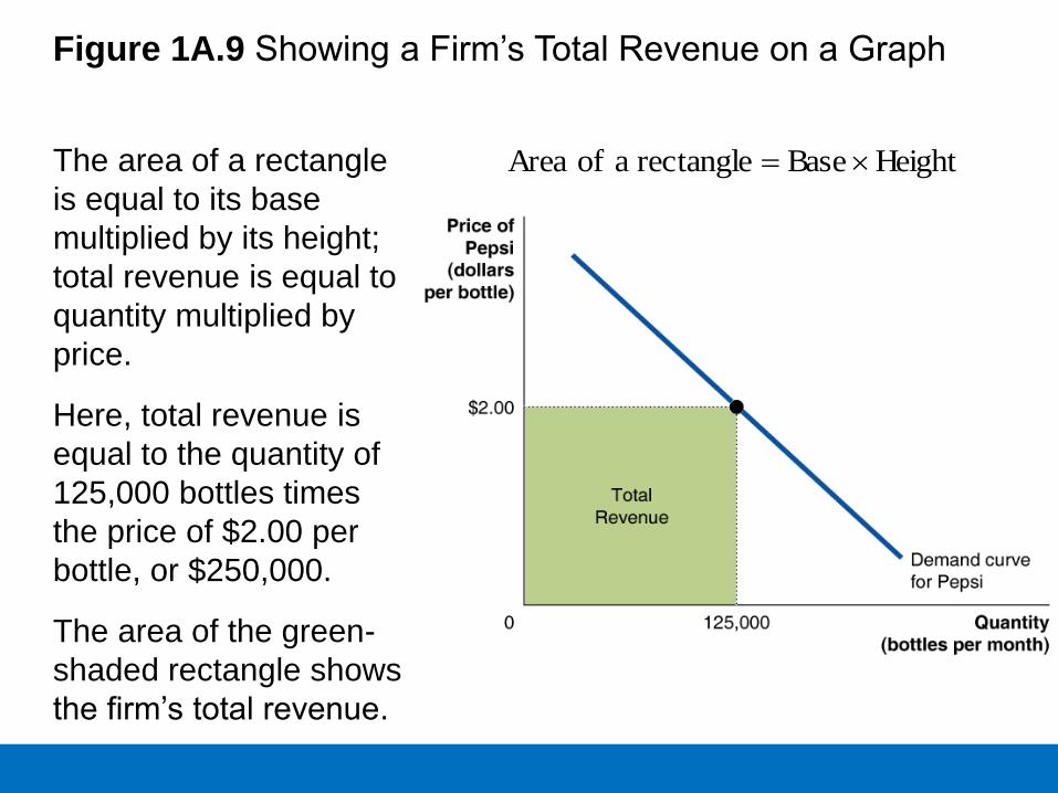
Figure 1A.9 Showing a Firm’s Total Revenue on a Graph

The area of a rectangle

is equal to its base

multiplied by its height;

total revenue is equal to

quantity multiplied by

price.

Here, total revenue is

equal to the quantity of

125,000 bottles times

the price of $2.00 per

bottle, or $250,000.

The area of the green-

shaded rectangle shows

the firm’s total revenue.

HeightBaserectangle a of Area

43

Figure 1A.10 The Area of a Triangle

The area of a triangle is

equal to ½ multiplied by

its base multiplied by its

height.

The area of the blue-

shaded triangle has a

base equal to

150,000 – 125,000, or

25,000, and a height

equal to $2.00 – $1.50,

or $0.50.

Therefore, its area

equals ½ 25,000

$0.50, or $6,250.

HeightBase2

1 trianglea of Area

44

Summary of Using Formulas

Whenever you must use a formula, you should follow these steps:

1. Make sure you understand the economic concept the formula

represents.

2. Make sure you are using the correct formula for the problem

you are solving.

3. Make sure the number you calculate using the formula is

economically reasonable. For example, if you are using a

formula to calculate a firm’s revenue and your answer is a

negative number, you know you made a mistake somewhere.