Priori Knowledge-Based Online Batch-to-Batch Identification in aClosed Loop and an Application to Injection MoldingZhixing Cao,†,‡ Yi Yang,¶ Hui Yi,† and Furong Gao*,†,§

†Department of Chemical & Biomolecular Engineering, Hong Kong University of Science & Technology, Clear Water Bay, Kowloon,Hong Kong‡Harvard John A. Paulson School of Engineering and Applied Sciences, Harvard University, Cambridge, Massachusetts 02138, UnitedStates¶Kunda Mold (Shenzhen) Company Ltd., Shenzhen 51800, China§Fok Ying Tung Research Institute, Hong Kong University of Science & Technology, Guangzhou, China

ABSTRACT: Online identification of a plant based on the input−output dataobtained under closed-loop operation conditions is a fundamental problem inmany industrial applications, because it paves the way for process monitoring,controller calibration, controller redesign, etc. This paper proposes a recursivebatch-to-batch identification method for modeling a batch process regulated by awithin-batch controller by exploiting its intrinsic repeatable pattern. Toovercome severe variations of parameter estimates, three kinds of priori plantknowledge are included, namely, time constant, static gain, and stability. Theconstraints formulated from priori plant knowledge are efficiently handled by atechnique−sequential projection. Additionally, the approach’s robustness againstinterbatch dynamics drift is analyzed mathematically. Finally, the performance ofthe proposed method is demonstrated on a numerical benchmark and a realindustrial application−injection molding.

1. INTRODUCTION

Online closed-loop identification is an important andfundamental problem in process control, because it depicts anevolutionary “map” to process control engineers for betterunderstanding the plant, also enabling further controllerupgrades such as redesigning controller parameters or set-points,1 or even implementation of advanced control strategiessuch as model predictive control (MPC)2−9 and adaptivecontrol.10−14 More than that, closed-loop identification extendsthe feasibility of the classical identification methods alreadyestablished for open-loop systems. It is well-known that, inreality, there are lots of scenarios that are impossible for open-loop identification. For example, an unstable process, whichalways has the unbounded tendency for almost any input signal,may compromise the open-loop identifiability condition; incontrast, with a stabilizing controller, closed-loop identificationcan achieve the modeling objective without endangering aplant’s normal operations. On the other hand, closed-loopidentification is much more challenging than open-loopidentification owing to the existence of the correlation betweenprocess noise and process input. Because of its importance andchallenges, many papers have contributed to closed-loopidentification in the past years. Roughly speaking, all theclosed-loop identification methods can be categorized intothree types according to the required data, namely, directapproach, indirect approach, and joint input−output ap-proach.15 Direct approach is a natural extension of open-loopidentification methods, as it formulates the regressor directly

based on the input−output data regardless of feedbackmechanism. Contrarily, the indirect approach requires theknowledge of controller structure, and feeds reference signaland process outputs to the algorithm. Unlike both of them, thejoint input−output approach augments process input andoutput as a new output and attempts to identify the augmentedsystem. The proposed method belongs to the indirectapproach.The contributions of this paper are 3-fold. The primary

contribution of this article is to develop an online closed-loopidentification algorithm particular for the batch process. In theclassic closed-loop identification literature, based on frequencyanalysis, Gustavsson, Ljung, and Soderstrom systematicallystudied the closed-loop identifiability problem;15−17 Miskovic and his colleagues discussed the reference excitation problemfor multivariable systems;18 Hjalmarsson and Gevers focusedon the experiment design of closed-loop identification;19,20

Forssell and Ljung surveyed the application of prediction errormethod in closed-loop identification;21 it has been reportedthat a two-stage method has been applied to a pilot-scaleprocess.22 On the basis of the time-domain analyticaltechniques, the effects of time delay and sampling time onthe identification results have been studied by Shardt and

Received: May 18, 2016Revised: July 5, 2016Accepted: July 23, 2016Published: July 24, 2016

Article

pubs.acs.org/IECR

© 2016 American Chemical Society 8818 DOI: 10.1021/acs.iecr.6b01900Ind. Eng. Chem. Res. 2016, 55, 8818−8829

Huang;23 Gilson and his co-workers developed a robustinstrumental variable(IV) method to the initialization step,24

and further extended the method to identify a continuous-timemodel based on sampled data;25 Huang, Ding, and Qin used aprojection subspace identification approach to eliminate thebias effect caused by the presence of feedback.26 However,identifying a batch-type plant is not a trivial task thanks to itsintrinsic nonlinearity and time variation;27 generally, directlyapplying these methods to a batch process may thereby notyield satisfactory results, for instance, a slow response tocapture intrabatch dynamics. Fortunately, the majority of batchprocesses are under repeated operations over a finite duration.This justifies changing the data processing and parameterestimates updating direction from time direction to batch/iteration direction, for example, changing from t − 1→ t to k −1 → k (t is the time index within a batch/iteration; k is thebatch/iteration index); it is quite similar to iterative learningcontrol (ILC), where control input is updated in the iterationdirection, for example, uk(t) = f [uk−1(t)].

28−30 To be specific,consider a simple scalar static system yk(t) = a(t)uk(t).Collecting the data in time direction gives {yk(1), uk(1), ...,yk(t), uk(t)}, in which the data contain distribution mismatch.On the contrary, organizing the data in iterations {y1(t), u1(t),..., yk(t), uk(t)} successfully avoids the distribution mismatch. Inshort, processing data along the iteration direction can beapproximately interpreted as handling independent identicaldistribution (i.i.d.) data. As to this point, similar research can befound in ref 31 in which an offline method was proposed; inrefs 32 and 33 the idea was incorporated with adaptive controlbut without studying transient performance; in refs 34 and 35only the open-loop cases have been discussed.Second, three different types of priori plant knowledge have

been translated into constraints to refine parameter estimates. Ithas been argued in papers 34−36 that directly changing thedata processing and estimates updating direction may give riseto undesired severe fluctuations on the parameter estimates,which somehow violates the common sense that dynamics ofchemical process are slowly varying. Thus, it necessitates theestimates refine procedure. The refinements are attained byimposing a set of constraints translated from priori plantknowledge, which are time constant, static gain, and stability.The first two can be obtained from a first-order-plus-time-delay(FOPTD) model, which is quite popular in practice.37 It is nottrivial to formulate the constraints on them, because theFOPTD model is in continuous time, while our identificationmodel is in discrete time. The stability knowledge is translatedinto dynamic constraints, which is updated in run-to-runfashion. All these constraints are efficiently handled by thesequential projection technique. Regarding this point, relevantliterature can be found: in ref 35 only the open-loopidentification problem has been investigated; in ref 36 onlythe closed-loop stability priori knowledge has been exploited.Third, the proposed algorithm is tested on a real industrial

application−injection molding. According to our knowledge, itis the first time that a linear time varying (LTV) model hasbeen identified on injection molding. In refs 38−40 it was onlyreported that a linear time invariant (LTI) model has beenestablished; in ref 41 a set-point based linear model wasidentified on injection molding.The remainder of this paper is organized as follows: section 2

presents the problem setup in closed-loop fashion; section 3gives the detailed identification method; section 4 formulatesthe priori plant knowledge into constraints and develops the

sequential projection for these constraints; section 5 analyzesthe algorithm’s robustness; section 6 studies the algorithm on anumerical example and a real industrial application−injectionmolding; section 7 draws a conclusion.

Notations: θ θ θ∥ ∥ = MMT is the Euclidean norm. The hat

(•) means estimation or something associated with estimates.T signifies transposition. f ◦ g(x) means the functioncomposition defined as f(g(x)). Polynomials are representedin uppercase italic symbols, i.e., A; matrices are expressed inuppercase bold symbols, i.e., A; vectors are in lowercase italicsymbols, i.e., x or θ. For two positive definite matrices A, B, A≻ B(A ≺ B) means A − B is a positive (negative) semidefinitematrix.

2. CLOSED-LOOP SYSTEMIn this paper, it is assumed that a batch-type plant can bedepicted by an autogressive exogenous (ARX) model, which is

= +− −A t q y t B t q u t e t( , ) ( ) ( , ) ( ) ( )k k k1 1

(1)

Here yk(t) and uk(t) are the process output and input,respectively. The subscript k is the iteration/batch index. tstands for the time index within an iteration. Denote L as theduration, and q−1 is the one-step backward shift operator intime. The disturbance and measurement noise can berepresented in ek(t). Following the standard identificationsetup, ek(t) is assumed to be a two-dimensional white noise.That is

σ= e j e n[ ( ) ( )]i m2

if and only if i = m and j = n; otherwise, it is equal to zero. Twodimensional white noise is a standard assumption in two-dimensional filtering; it represents the worst scenario that thenoise has effects on the entire frequency domain. A(t, q−1) andB(t, q−1) are time-varying polynomials in the form of

= + + +

+

− − −

−

A t q a t q a t q

a t q

( , ) 1 ( ) ( )

... ( )nana

11,0

12,0

2

,0 (2a)

= + + +− − − −B t q b t q b t q b t q( , ) ( ) ( ) ... ( )nbnb1

1,01

2,02

,0

(2b)

where na and nb are the orders of the three polynomials 2a−2b.The coefficients a1,0, ..., ana,0 and b1,0, ..., bnb,0 : → L[0, ] aretime-varying real functions. Hereby we have assumed that thedelay order is equal to 1; in fact, this assumption does not loseany generality, because it can be addressed by letting the first d− 1 terms in eq 2b be equal to zeros. In addition, the timevariations arise from the repeated operations in the proximity ofa certain operation profile, which may roughly make a nonlinearsystem reduce to an LTV system. To be specific, consider asystem y = G(t, u) regulated to follow an operating line ur,which is a function of time t. Under a relatively good regulation,the closed-loop dynamics can be approximated by a linearizedmodel

− = − ≈ ∂∂

| −y y G t u G t uGu

u u( , ) ( , ) ( )r r u rr

where |∂∂Gu ur

is a function of time t. This justifies the LTV ARX

model assumption with a relatively good controller.

Industrial & Engineering Chemistry Research Article

DOI: 10.1021/acs.iecr.6b01900Ind. Eng. Chem. Res. 2016, 55, 8818−8829

8819

As for the controller, it assumes that the plant (1) isregulated under an R−S−T controller, a two-degree-of-freedomcontroller, whose explicit form is given as

= − +−

−

−

−u tR qS q

y tT qS q

r t( )( )( )

( )( )( )

( )k k k

1

1

1

1(3)

It is noted that the PID controller can be easily accommodatedin this type. Actually, the controller is quite general, and hasbecome a standard assumption in closed-loop identification.42

The rk(t) in eq 3 is the reference signal; it comprises two parts:one is the repeatable part (the operation profile rr(t)), the otheris the nonrepeatable part to provide sufficient excitation, rnr,k(t).To be specific, it is

= +r t r t r t( ) ( ) ( )k kr nr, (4)

Furthermore, it is assumed that S(q−1) is in the canonical formwhose constant term is equal to 1, that is, S(q−1) = 1 +q−1S*(q−1). It does not lose any generality; it is convenient totransform noncanonical into canonical form by simple scaling.Thereafter, the control law can be summarized as

=u t f y t( ) ( ( ))k k

a function of yk(t).

3. IDENTIFICATION METHODSWith the basics defined, we are ready to present theidentification method. Basically, it includes two components:predictor and estimator. The predictor is used to generateoutput prediction, that is, yk(t), while the estimator is used toyield parameter estimates by minimizing the output predictionerror, that is, yk(t) − yk(t).3.1. Predictor. To keep the notations neat, the shift

operator q−1 will be dropped out in the remainder of the paperwithout any ambiguity. From eqs 1 and 3, the closed-loopdynamics of the plant is

= − * + +y t A t y t B t u t e t( ) ( ) ( ) ( ) ( ) ( )k k k k

where A(t) = 1 + A*(t). A*(t) contains the terms with at leastone unit backward shift. It can also be written in linearregression form:

ϕ θ= +y t t e t( ) ( ) ( )k k kT

0 (5a)

ϕ = − − − − −

−

t y t y t na u t

u t nb

( ) [ ( 1) ... ( ) ( 1)

... ( )]

k k k k

k

T

(5b)

θ =t a t a t b t b t( ) [ ( ) ... ( ) ( ) ... ( )]0T

1,0 na,0 1,0 nb,0

(5c)

Given the parameter estimates, the output prediction yk(t) isgenerated by

φ θ = y t t t( ) ( ) ( )k k kT

(6a)

φ = − − − − −

−

t y t y t na u t

u t nb

( ) [ ( 1) ... ( ) ( 1)

... ( )]

k k k k

k

T

(6b)

θ = t a t a t b t b t( ) [ ( ) ... ( ) ( ) ... ( )]k k na k k nb kT

1, , 1, ,

(6c)

where uk(t) is the control input based on the prediction yk(t),namely u k(t) = f(yk(t)) = −Ryk(t)/S + Trk(t)/S. Note that,basically, the predictor in eq 6 proposed by Landau et al.replicates the plant dynamics but based on the predictions andparameter estimates only, shown in Figure 1. Define the outputerror

ϵ ≔ − t y t y t( ) ( ) ( )k k k

Then, one rewrites eq 5a as

φ θ ϕ φ θ= + −y t t t t t( ) ( ) ( ) [ ( ) ( )]k k k kT

0T

0

Figure 1. Predictor structure.

Industrial & Engineering Chemistry Research Article

DOI: 10.1021/acs.iecr.6b01900Ind. Eng. Chem. Res. 2016, 55, 8818−8829

8820

Since −yk(t) + yk(t) = −ϵk(t) and uk(t) − u k(t) = −Rϵk(t)/S, itcan be further simplified to

φ θ= − * + ϵy t t t A t B t R S t( ) ( ) ( ) [ ( ) ( ) / ] ( )k k kT

0

Combining with eq 6, one can get

φ θ θϵ = − +

− * + ϵ

t t t t e t

A t B t R S t

( ) ( )[ ( ) ( )] ( )

[ ( ) ( ) / ] ( )

k k k k

k

T0

It is equivalent to

φ θϵ = − +H t t S t t e t( ) ( ) [ ( ) ( ) ( )]k k k kT

(7)

where H(t) ≔ A(t)S + B(t)R is the closed-loop characteristicpolynomial, which decides the closed-loop stability. The minussign arises from the definition θk(t) ≔ θk(t) − θ0. To justify thepredictor, letting θk(t) = θ0, which suggests that for a boundednoise ek(t), the output prediction error ϵk(t) will converge toek(t) as t → ∞.3.2. Estimator. It is known that identification problems are

usually translated into an empirical optimization problem suchas minimizing the output prediction error. Therefore, how toformulate the associated cost function is of great importance. Inthe conventional identification methods, the cost function isselected as the summation of the output prediction error alongthe time t. This choice is not wise in the case of a time-varyingplant, since all the data {yk(1), φk(1), ..., yk(t), φk(t)} are drawnfrom different distributions caused by a time variation of theplant. That may give rise to the failure of converging to the truemodel, that is, θ0. This problem is easily circumvented byswitching the summation direction from time t to iteration k.That means instead of solving a single optimization problem,we solve a set of optimization problems differentiated by time t;and at each time t, the data {y1(t), φ1(t), ..., yk(t), φk(t)} can beapproximately regarded as i.i.d. drawn from the samedistribution. Specifically, at each time t, we attempt to minimizethe cost function

∑ φ θ= − =

J t y t t( ) [ ( ) ( ) ]ki

k

i i1

T 2

Invoking Newton’s methods,17,34 it is easy to arrive at

θ θ φ θ = + − − −t t K t y t t t( ) ( ) ( )[ ( ) ( ) ( )]k k k k k k1

T1 (8a)

φφ φ

=+

−

−K t

P t t

t P t t( )

( ) ( )

1 ( ) ( ) ( )kk k

k k k

1T

1 (8b)

φ φφ φ

= −+−

− −

−P t P t

P t t t P t

t P t t( ) ( )

( ) ( ) ( ) ( )

1 ( ) ( ) ( )k kk k k k

k k k1

1T

1T

1 (8c)

It is similar to eq 15 and 16 in ref 34, but here we use a differentregressor φk(t) which only relies on the past predictions yk(t),u k(t), rather than past outputs yk(t), uk(t).

4. ESTIMATE REFINEMENTAs argued in refs 34−36 a direct employment of eq 8 cannotyield a “smooth” parameter estimate that may result in anunsatisfactory real dynamics tracking but still with good outputprediction capabilities. In practice, such model fluctuations maygive rise to frequent controller action for some model-basedcontrol policies, thus perhaps degrading control performance.However, in the traditional recursive least-squares (RLS)

identification algorithm, such parameter estimate fluctuationsare not often seen. Even in mathematics, it can be proven thatthe traditional RLS has an inherent smoothing effect; that is∥θk(t) − θk(t − 1)∥ → 0 even ∥θk(t + i) − θk(t)∥ → 0 for anarbitrary positive integer i as t → ∞.43 The possible reasonresponsible for these undesired fluctuations is that there do notexist strong relations between the data in different iterations k,for instance, φk(t) and φk−1(t), due to the i.i.d. sampling. But interms of time t, the regressors at different times are governed bysome difference equation. For example, due to the existence ofplant dynamics, there must exist a transition matrix t( ) andan input vector ηk(t) such that

φ φ η= − +t t t t( ) ( ) ( 1) ( )k k k

which in nature is a low-pass filter with smoothing effect. Withthis understanding, an intuitive solution is to impose somesensible constraints to restrict the estimate fluctuations.In this section, we are going to formulate these constraints

based on priori plant knowledge. Nevertheless, practically, itmay lack computationally efficient methods to solve theconstrained optimization problem, therefore making onlineidentification infeasible. Since new measurements are con-tinuously coming, it is more important to find an efficientsuboptimal solution to accommodate the new measurementsthan seek an optimal solution at each time. Projecting anunconstrained optimizer onto a closed feasible domain is aplausible approach for suboptimal solution seeking. Mathemati-cally speaking, given a feasible domain Θ constructed frompriori plant knowledge, the projection step is to find

θ θ θ ∈ ∥ − ∥θΘ ∈Θ

t tProj [ ( )] arg min ( )k k

This step is easy to implement if the domain Θ is geometricallysimple, for example, ball, polygon, cube, etc.Section 4.1 formulates three types of priori plant knowledge

into various constraints. Section 4.2 proposes an efficientapproach to solve the constrained optimization problem basedon sequential projection.

4.1. Priori Knowledge Formulation. In this subsection,we focus on constraints formulation of priori plant knowledge.Three types of priori plant knowledge will be discussed,namely, time constant, static gain, and stability. The first twotypes are the key elements of a FOPTD transfer functionmodel; that is,

τ=

+

τ−G s

Ks

( )e

1

sd

Here K, τd, and τ are the static gain, time delay, and timeconstant, respectively. The FOPTD model plays a crucial rolein process control, since it provides important guidance for PIDor IMC (internal model controller) tuning.37 Note that ourplant has been already operated in closed loop; this implies thatan FOPTD model is probably ready for use. Hence, it is notrisky or restrictive to assume its existence. It should beremarked that the FOPTD model is a continuous-time model,whereas the ARX model is in discrete time. It is not trivial totranslate the knowledge of time constant and static gain intoconstraints imposed on the estimates of the ARX model. Onthe other hand, process stability widely exists in industry,thanks to various physicochemical conservation laws, whichmake the assumption on it not lose generality either. Unliketime constant or static gain, the stability constraint can be

Industrial & Engineering Chemistry Research Article

DOI: 10.1021/acs.iecr.6b01900Ind. Eng. Chem. Res. 2016, 55, 8818−8829

8821

established in discrete time with the help of the Lyapunovequation.4.1.1. Time Constant. It is well-known that the FOPTD

model is usually a reduced-order model approximating theoriginal high-order dynamics. There are many methodscontributing to this topic, such as Taylor series approximationand Skogestad’s half rule.37,44 Assume that the original plant hasthe dynamics represented by

τ=

∏ +=G s

F ss

( )( )

( 1)ina

i1

where F(s) is a polynomial of s. The sequence {τi} is anonincreasing sequence, that is, τ1 ≥ τ2 ≥ ··· ≥ τna. Note thatdue to exact knowledge of process order, the order na of ARXmodel has to be consistent with the number of terms in theproduct of G(s). Decomposing G(s) into several first-orderterms gives

∑τ

=+=

G sf

s( )

1/i

nai

i1

for some f i. Discretizing G(s), one can have

∑=−

= ′∏ −τ τ

−

=−

=−G z

f F z( )

1 e( )

(1 e )i

nai

Tina T

1

1/

1/i i

for some F′(z). Therefore, the following relation can beestablished.

∑= − τ

=

−a t( ) ei

naT

11

/ i

where T is the sampling time. It remains to find appropriateupper and lower bounds of the summation ∑i = 1

na e−T/τi. Noticethat the function g(x) = exp(−T/x) is a monotonicallyincreasing function and τ ≥ τ1. Therefore, a reasonable lowerbound for a1(t) is − (na)e−T/τ.On the other hand, according to Skogestad’s half rule,44 the

lower bound of the largest time constant τ2 is

τ τ τ τ τ τ τ+ = < + ⇔ </2 /2231 2 1 1 1

Hence, a heuristic upper bound for a1(t) is − (na)e−3T/(2τ). Bynow, we have obtained an interval for a 1,k(t), which is

∈ − −τ τ− −a t na: ( ) [ ( )e , (na)e ]kT T

1 1,/ 3 /(2 )

4.1.2. Static gain. Recall the definition of static gain, that is

= y Ku

where y is the steady-state output under constant input u .According to eq 1, we have

∑ ∑+ = = =

a y b u(1 ) ( )i

na

ii

nb

i1 1

It indicates that K = (∑i = 1nb bi)/(1 + ∑i = 1

na ai). Given 100%variation on K, the heuristic bound can be given as

∑ ∑

∑ ∑

− + ≤

− + ≥

= =

= =

⎧

⎨⎪⎪⎪

⎩⎪⎪⎪

b t K a t

b t K a t

:

( ) 2 [1 ( )] 0

( ) 0.5 [1 ( )] 0

i

nb

i ki

na

i k

i

nb

i ki

na

i k

21

,1

,

1,

1,

4.1.3. Stability. In contrast to the aforementioned two kindsof constraints, the stability constraint will be given as a normball whose size is updated in real time. This kind of constraintshas been studied in Cao et al.35 To be concise, only thebackbone will be presented; for more details, please refer to ref35. For every parameter estimate θk(t), there exists acorresponding state matrix; that is,

θ ∼

=

− − − −

⋮ ⋱ ⋮ ⋮

− −⎡

⎣

⎢⎢⎢⎢⎢⎢

⎤

⎦

⎥⎥⎥⎥⎥⎥

t t

a t a t a t a t

A( ) ( )

( ) ... ( ) ( ) ( )

1 0 ... 0 00 1 ... 0 0

00 0 ... 1 0

k k

k na k na k na k1, 2, 1, ,

Suppose that θk−1(t) satisfies the stability constraint; to beprecise, ρmax [Ak−1(t)] < η < 1, where η is the priori modulusupper bound of the largest eigenvalue. According to theLyapunov theorem, for identify matrix, there exists a positivedefinite matrix Mk(t) such that

η − = −− −t t t tA M A M I( ) ( ) ( ) ( )k k k k1 1T 2

(9)

If we want to ensure θk(t) satisfying stability constraint, orequivalently, Ak(t) is stable, it has to guarantee that

δ δ

η

+ +

− ≺− −t t t t t t

t

A A M A A

M

[ ( ) ( )] ( )[ ( ) ( )] ( )

( ) 0k k k k k

k

1 1T

2(10)

with δAk(t) ≔ Ak(t) − Ak−1(t). It is noticed that it is a standardsetup in robust control theory. By robust parametrization, thesufficient condition for eq 10 is

η

δ δ

ϵ − + ϵ

+ + ϵ ≺

− −t

t t t

M I

A M A

( ) (1 )

(1 ) ( ) ( ) ( ) 0k

k k k

1 2 1

T

Note that there exists a relation that δAk(t)Mk(t)δAk =diag{∥δθA,k(t)∥Mk(t)

2 , 0(na−1)×(na−1)}, where δθA,k(t) is the firstna elements of δθk(t). Based on that, maximizing∥δθA,k(t)∥Mk(t)

2 , one can have

δθ

η λ η η λ λ

Δ ≔ ∥ ∥

=− + −

t t

t t tM M M

( ) max ( )1

2 [ ( )] 1 2 ( [ ( )] 1) [ ( )]

k A k t

k k k

M, ( )2

2max

2max max

k

(11)

In this way, the stability constraints have been translated into aweighted 2-norm ball whose center is the previous parameterestimate θk−1(t). The size of the ball is controlled by eq 11. Tosummarize, the constraints can be written in the followingcompact form:

θ θ θ θ ∈ |∥ − ∥ ≤ Δ−t t t: ( ) { ( ) ( )}k A k A k t kM3 , , 1 ( )2

k

Remark 1: Note that the constraints ,1 2 are staticconstraints so that they can be computed offline; the constraint

Industrial & Engineering Chemistry Research Article

DOI: 10.1021/acs.iecr.6b01900Ind. Eng. Chem. Res. 2016, 55, 8818−8829

8822

3 is a dynamic constraint so that it needs updating; that makesit a standard trust region method,45 where Δk(t) is the size oftrust region. In the updating procedure, it is not computation-ally cheap to solve Mk(t) in the Lyapunov equation; however,the computation of Mk(t) and Δk(t) can be implemented inparallel with the identification procedure (also can be calculatedin the resettling time of batch process).Remark 2: It is worthy remark that FOPTD model is only

used for estimate refinement not the identification objective toachieve. Additionally, we do not impose any constraint on themodel dimension; it does not have to be the first-order model.Admittedly, it is relatively easy to solve the optimizationproblem with the time constant and static gain constraints bythe means of a direct optimization method; but the stabilityconstraint is not computational friendly for direct optimizationin real time, because it is nonconvex as argued in our previouspaper.35 This can be seen from eq 9, which contains a productof two optimization variables Ak−1(t) and Mk(t). Thus, itmotivates the usage of projection method detailed in thefollowing section.4.2. Sequential Projection. In the above subsection, the

priori plant knowledge on time constant, static gain, andstability has been turned into constraints, namely , ,1 2 3.Further note that 1 delineates an interval on real axis denotedas Θ

1; 2 describes a space supported by two hyperplane

denoted as Θ2; 3 depicts a norm ball in space +na nb,

denoted as Θ3. Hence, the projection step turns to be

θ θ θ = ∥ − ∥θΘ ∩Θ ∩Θ ∈Θ ∩Θ ∩Θ

t tProj [ ( )] arg min ( )k k1 2 3

1 2 3

Although every space Θ1, Θ

2or Θ

3is geometrically simple

enough, their intersection can be quite complex, perhapsmaking the projection step computationally intractable.Fortunately, recall that the primary goal of our problem is touse proper constraints to mitigate the estimates variationsefficiently rather than to attain the optimality of thecorresponding projection step. Bearing that in mind, anintuitive efficient approximation of the aforementionedprojection operator is

θ θ

θ

θ

≔

≔ ◦ ◦

≈ Θ Θ Θ

Θ ∩Θ ∩Θ

t t

t

t

( ) Proj[ ( )]

Proj Proj Proj [ ( )]

Proj [ ( )]

kR

k

k

k

3 2 1

1 2 3 (12)

Thereafter, since every step the estimate projects onto ageometrically simple space, it is efficient to compute thisapproximation. This approach is named sequential projection.Remark 3: The first thing should be remarked is that the

sequential projection does not guarantee the constraintsatisfaction of 1 or 2. However, this does not matter much,owing to two reasons. First, the constraints 1 and 2 areformulated semiheuristically; strongly sticking to them may ruleout the true parameter set. Second, constraint satisfaction is notthe primary goal either; the main concern here is to find anefficient method for online implementation.Remark 4: Different orders of Θ Θ,

1 2and Θ

3may yield

different projection results. Thus, the order may affect the finalestimation performance. A plausible rule of thumb is that ofplacing the concrete constraint outside and putting the heuristicone inside. It is based on the philosophy that the outside

constraints have been formulated with stronger confidence sothat they have to be satisfied more strictly. In our case, thestability constraint is the most confident one, because thereexists a step response; that makes it the most outside one.Now it remains to figure out each projection step in eq 12.

Then, for 1, we have for any ∈ +x na nb

=

− < −

− ≤ < −

− ≤ −

τ τ

τ τ

τ τ

Θ

−

−

− −

−

−

⎧

⎨⎪⎪

⎩⎪⎪

x

x x

x x

x x

Proj ( )

[ (na)e , ] , (na)e

, (na)e (na)e

[ (na)e , ] , (na)e

Ta a

T

Ta

T

Ta a

T

/ T T /

/ 3 /(2 )

3 /(2 ) T T 3 /(2 )1

1 1

1

1 1

(13)

where xa1 stands for the first element of x and xa¯1 means the lastna + nb − 1 elements of x. Note 3 imposes a constraint on thefirst na elements of θk(t) ; 2 can be used to impose on the lastnb elements of θk(t).

=

< +

+ ≤ < +

* ≥ +Θ

+ +

+ + +

+ +

★⎧⎨⎪⎪

⎩⎪⎪

x

x x x K x

x K x x K x

x x x K x

Proj ( )

[ , ] , 0.5 (1 )

, 0.5 (1 ) 2 (1 )

[ , ] , 2 (1 )

a b b a

a b a

a b b a

T T T

T T T2

(14)

where xa+, xb+ mean the summations of all the first na and allthe last nb elements of x respectively. xa stands for the vectorthat contains the first na elements of x. xb★ and xb* are definedas

=+ +

+★

xK x

xx

0.5 (1 )b

a

bb

and

=+

*+

+x

K xx

x2 (1 )

ba

bb

xb is the vector comprising the last nb elements of x. As for theprojection of 3, it is a projection on to a norm ball. So weparticularly introduce the norm ball projection operator as

α= + −Θ x z t x z xProj ( ) [ ( )( ), ]za k a a b

T T

3 (15a)

α =

∥ − ∥ ≤ Δ

Δ∥ − ∥

⎧⎨⎪⎪

⎩⎪⎪

t

x z t

tx z

( )

1, ( )

( ), otherwisek

a a t k

k

a a t

M

M

( )

( )

k

k (15b)

Here z is the center of the norm ball. Additionally, za, atpresent, means the first na elements of θk

R(t) or θ − tProj[ ( )]k 1 .

Later, we will introduce another version of z. Up to now, theconstraints based priori plant knowledge have been formulated;their corresponding efficient solving approaches have all beenpresented.

5. ROBUST ANALYSISIt is well-known that a batch process may exhibit slowinterbatch dynamic drift, which arises from facilities aging oraccumulation of residual reactants.27 Therefore, it is importantto investigate the robustness of the proposed identificationalgorithm against interbatch dynamics drift. Consider that

= +− −A t q y t B t q u t d t( , ) ( ) ( , ) ( ) ( )k k k1 1

(16)

Industrial & Engineering Chemistry Research Article

DOI: 10.1021/acs.iecr.6b01900Ind. Eng. Chem. Res. 2016, 55, 8818−8829

8823

where dk(t) represents the effect of model-plant mismatch anddisturbances. This setup is quite general, and widely used inidentification literature, for instance Landau et al.42 The robustanalysis studies, given dk(t) and the reference rk(t) are normbounded, are used to determine the boundedness of yk(t) andposterior prediction error yk(t) − φk

T θkR(t). Obviously, dk(t) has

absorbed the noise term ek(t).Theorem 1: Consider the plant represented in eq 16 and the

parameter estimates generated by algorithm in eq 8 togetherwith estimate refinement procedures eqs 13−15. Assume that

A1. the order of the plant na, nb are exactly known,A2. the controller (3) stabilizes the plant (16),A3. the reference rk(t) and unmodeled plant dynamics dk(t)

are both bounded in the sense that there exist Cr1, Cr2,Cr3, Cr4 ∈ (0, + ∞) such that

∑ ≤ +=

r t C K C( )i

K

i r r1

21 2

and

∑ ≤ +=

d t C K C( )i

K

i d d1

21 2

for any K and uniformly for all t,A4. all the priori constraints , ,1 2 3 cover the real

parameter set θ0,A5. there exists a positive real number μ > 1 such that

μ−SH t( ) 2

is strictly positive real and stable uniformly for all t.

Then, there exists Cp1, Cp2, Ce1, Ce2 ∈ (0, + ∞) such that

∑ ≤ +=

y t C K C( )i

K

i p p1

21 2

and

∑ φ θ− ≤ +=

y t t t C K C[ ( ) ( ) ( )]i

K

i i kR

e e1

T 21 2

for any K and uniformly for all t.Proof: Since the proof is quite technical, please refer to

Appendix A for details.

6. NUMERICAL EXPERIMENT

6.1. Adaptive Filter. The imposition of the constraints, ,1 2 3 will reduce the magnitude of fluctuation on the

estimates; in practice, in order to further improve thesmoothness, it is suggested to employ the following adaptivefilter:35

θ

γθ γ θθ θ κ κ κ

γ θ γ θ

=

+ − −∥ − − ∥ ≥ +

+ − −

⎧⎨⎪⎪

⎩⎪⎪

t

t t

t t

t t

( )

( ) (1 ) ( 1),

( ) ( 1)

( ) (1 ) ( 1), otherwise

kf

kR

kf

kR

kf k

kR

kf

1 1

1 2 3

2 2

(17)

It is a low-pass filter. γ1 and γ2 are positive real numbersbetween 0 and 1. κ1, κ2, and κ3 are all positive real numbers; κ3is between 0 and 1. It is suggested that the γ2 should have astronger smoothing effect to neutralize the small-magnitudefluctuations; that means γ2 should be smaller than γ1. κ1 shouldbe closer to the maximum dynamics change within an iteration.κ2 and κ3 are two tuning knobs for the filter; they have adecaying effect on the filter switch threshold. The goal ofintroducing them is to allow the algorithm to aggressivelypursue minimizing the prediction error at first and graduallyswitch to pursue smoothing estimates later. According toexperiences, γ1 is usually selected between 0.7 and 0.9, while γ2is chosen between 0.2 and 0.5. κ2 is usually selected as 1.2κ1; κ3is between 0.7 and 0.9. The filter is organized in a convexcombination form to avoid massive violations of the constraints

3; the trust region calculation part can handle the violation byrejecting the filtered version but keep using θk−1

f (t). Then,

Figure 2. Identification results comparison among Landau’s method, conventional method, and the proposed method.

Industrial & Engineering Chemistry Research Article

DOI: 10.1021/acs.iecr.6b01900Ind. Eng. Chem. Res. 2016, 55, 8818−8829

8824

another version of z in eq 15a will be θkf (t). The whole

proposed algorithm has been summarized in Appendix B.6.2. Example 1. In this part, we consider the adapted

example from Example 1 in Laudau and Karimi’s work.42 Thesystem is set up as follows:

=

− + ∈

+ − + × − +

∈

− + ∈

−

− −

− −

− −

⎧

⎨⎪⎪⎪

⎩⎪⎪⎪

⎡⎣⎢

⎤⎦⎥A z

z z t

t z z

t

z z t

( )

1 1.5 0.7 , [0, 150)

1 1.50.32150

( 150) 0.7 ,

[150, 300)

1 1.18 0.7 , [300, 600]

1

1 2

1 2

1 2

=+ ∈

+ ∈−

− −

− −⎪

⎪⎧⎨⎩

B zz z t

z z t( )

0.5 , [0, 150)

0.9 0.5 , [150, 600]1

1 2

1 2

The R-S-T controller is chosen as

= − +

= − −

− − −

− − −

R z z z

S z z z

( ) 0.8659 1.2763 0.5204

( ) 1 0.6283 0.3717

1 1 2

1 1 2

The system A(z−1), B(z−1) is regulated by the controllerR(z−1), S(z−1) repeatedly over a finite period t ∈ [0,600]. λk, η,γ1, γ2, κ1, κ2, and κ3 are respectively chosen as 0.98, 0.9, 0.7, 0.3,0.8, 1.25, and 0.8. The reference signal is selected as a stepchange from 0.5 to −0.5 at time 150. The unrepeatable partrnr,k(t) in eq4 is designed as the PRBS (pseudorandom binarysequence) with magnitude of 0.3. The white noise variance is0.2. The priori time constant and static gain are 0.8 and 5,respectively. We use Landau’s method to initialize thealgorithm (identify the first iteration/batch).42 Figure 2 showsthe identification results of three different methodsLandau’smethod (Figure 2a,d), conventional method in eq 8 (Figure2b,e), and the proposed method (Figure 2c,f). In Figure 2, theblue solid line represents the estimates; the red dash line standsfor the true parameter. It clearly shows that not changing dataprocessing or estimate updating direction yields a slow trackingresponse. It also indicates that the proposed method cansignificantly reduce the fluctuations on the estimates. Figure 3 is

the logarithm plot of the PTE comparison. PTE is short forparameter tracking error.35 Its definition is PTE = ∑t = 1

L ∥θk(t)− θ0(t)∥2. The blue line is the result of directly applying theconventional method (eq 8); the orange line represents theresult with the stability constraints 3 (SC) applied; themagenta line is the result with both stability constraints 3 andfirst-order constraints ,1 3 (FCSC) applied; the red line is theresult of the proposed method with filter and , ,1 2 3 applied

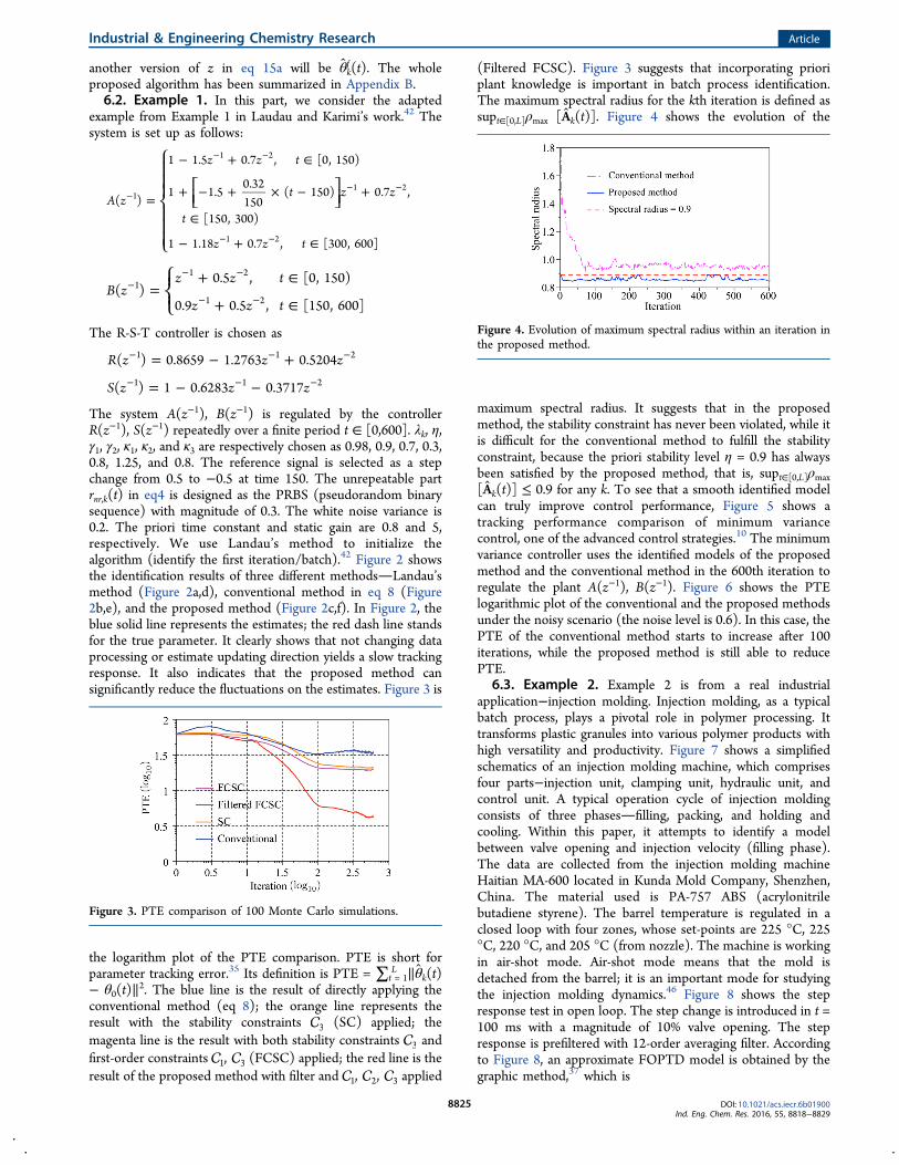
(Filtered FCSC). Figure 3 suggests that incorporating prioriplant knowledge is important in batch process identification.The maximum spectral radius for the kth iteration is defined assupt∈[0,L]ρmax [Ak(t)]. Figure 4 shows the evolution of the

maximum spectral radius. It suggests that in the proposedmethod, the stability constraint has never been violated, while itis difficult for the conventional method to fulfill the stabilityconstraint, because the priori stability level η = 0.9 has alwaysbeen satisfied by the proposed method, that is, supt∈[0,L]ρmax[Ak(t)] ≤ 0.9 for any k. To see that a smooth identified modelcan truly improve control performance, Figure 5 shows atracking performance comparison of minimum variancecontrol, one of the advanced control strategies.10 The minimumvariance controller uses the identified models of the proposedmethod and the conventional method in the 600th iteration toregulate the plant A(z−1), B(z−1). Figure 6 shows the PTElogarithmic plot of the conventional and the proposed methodsunder the noisy scenario (the noise level is 0.6). In this case, thePTE of the conventional method starts to increase after 100iterations, while the proposed method is still able to reducePTE.

6.3. Example 2. Example 2 is from a real industrialapplication−injection molding. Injection molding, as a typicalbatch process, plays a pivotal role in polymer processing. Ittransforms plastic granules into various polymer products withhigh versatility and productivity. Figure 7 shows a simplifiedschematics of an injection molding machine, which comprisesfour parts−injection unit, clamping unit, hydraulic unit, andcontrol unit. A typical operation cycle of injection moldingconsists of three phasesfilling, packing, and holding andcooling. Within this paper, it attempts to identify a modelbetween valve opening and injection velocity (filling phase).The data are collected from the injection molding machineHaitian MA-600 located in Kunda Mold Company, Shenzhen,China. The material used is PA-757 ABS (acrylonitrilebutadiene styrene). The barrel temperature is regulated in aclosed loop with four zones, whose set-points are 225 °C, 225°C, 220 °C, and 205 °C (from nozzle). The machine is workingin air-shot mode. Air-shot mode means that the mold isdetached from the barrel; it is an important mode for studyingthe injection molding dynamics.46 Figure 8 shows the stepresponse test in open loop. The step change is introduced in t =100 ms with a magnitude of 10% valve opening. The stepresponse is prefiltered with 12-order averaging filter. Accordingto Figure 8, an approximate FOPTD model is obtained by thegraphic method,37 which is

Figure 3. PTE comparison of 100 Monte Carlo simulations.

Figure 4. Evolution of maximum spectral radius within an iteration inthe proposed method.

Industrial & Engineering Chemistry Research Article

DOI: 10.1021/acs.iecr.6b01900Ind. Eng. Chem. Res. 2016, 55, 8818−8829

8825

=+

−G s

s( )

1.16e70 1

s30

with millisecond as time unit. Afterward, 80 closed-loop PRBStests are conducted. The duration of a cycle (iteration) is 2 s;the sampling period is 10 ms. The injection velocity iscontrolled by PID in velocity form; that is, R = S = T = 1 − q−1.The control block diagram is shown in Figure 9. The loop ofvalve opening to injection velocity is closed, and valve openingis the manipulated variable. The reference is 60 mm/s on andbefore time t = 100 and 40 mm/s afterward. The magnitude ofPRBS on reference is 6 mm/s. Since the step response test isintroduced in t = 100 and in the beginning of each cycle, theinjection molding system is not very steady. Also recalling thatinjection molding has strong time variations,39 it is reasonable

to impose ,1 2 over the last 2/3 duration. η, γ1, γ2, κ1, κ2, κ3are selected as 0.9, 0.7, 0.5, 0.8, 1.25, 0.8, respectively.According to the literature,39 the order is chosen as na = 1,nb = 2, nd = 3. Figure 10 shows the comparison of identificationresults. It suggests that the prediction ability of Landau’smethod does not improve from iteration to iteration, but the

Figure 5. Minimum variance control results based on the identification of the proposed method and the conventional method.

Figure 6. PTE comparison of 100 Monte Carlo simulations for noisydata.

Figure 7. Simplified schematics of injection molding machine39

Figure 8. Step response of injection velocity (IV) vs valve opening(VO).

Figure 9. Diagram of closed-loop control block of Example 2.

Industrial & Engineering Chemistry Research Article

DOI: 10.1021/acs.iecr.6b01900Ind. Eng. Chem. Res. 2016, 55, 8818−8829

8826

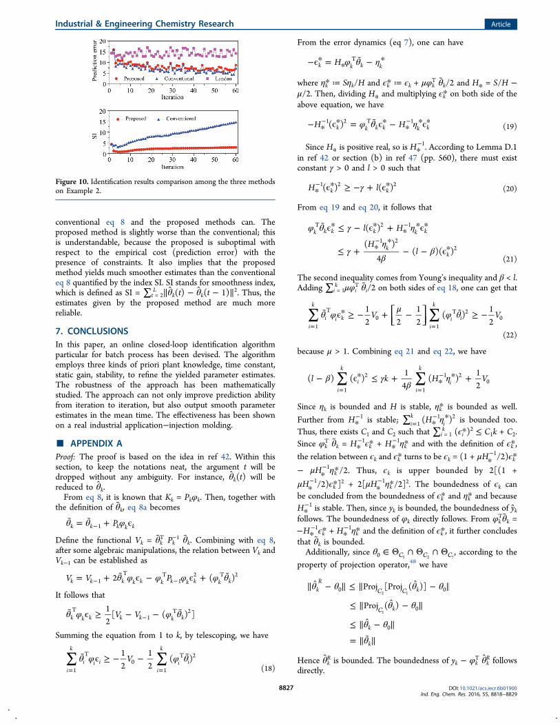
conventional eq 8 and the proposed methods can. Theproposed method is slightly worse than the conventional; thisis understandable, because the proposed is suboptimal withrespect to the empirical cost (prediction error) with thepresence of constraints. It also implies that the proposedmethod yields much smoother estimates than the conventionaleq 8 quantified by the index SI. SI stands for smoothness index,which is defined as SI = ∑t = 2

L ∥θk(t) − θk(t − 1)∥2. Thus, theestimates given by the proposed method are much morereliable.

7. CONCLUSIONSIn this paper, an online closed-loop identification algorithmparticular for batch process has been devised. The algorithmemploys three kinds of priori plant knowledge, time constant,static gain, stability, to refine the yielded parameter estimates.The robustness of the approach has been mathematicallystudied. The approach can not only improve prediction abilityfrom iteration to iteration, but also output smooth parameterestimates in the mean time. The effectiveness has been shownon a real industrial application−injection molding.

■ APPENDIX AProof: The proof is based on the idea in ref 42. Within thissection, to keep the notations neat, the argument t will bedropped without any ambiguity. For instance, θk(t) will bereduced to θk.From eq 8, it is known that Kk = Pkφk. Then, together with

the definition of θk, eq 8a becomes

θ θ φ = + ϵ− Pk k k k k1

Define the functional Vk = θkT Pk

−1 θk. Combining with eq 8,after some algebraic manipulations, the relation between Vk andVk−1 can be established as

θ φ φ φ φ θ= + ϵ − ϵ + − −V V P2 ( )k k k k k k k k k k k1

T T1

2 T 2

It follows that

θ φ φ θ ϵ ≥ − − −V V

12

[ ( ) ]k k k k k k kT

1T 2

Summing the equation from 1 to k, by telescoping, we have

∑ ∑θ φ φ θ ϵ ≥ − − = =

V12

12

( )i

k

i i ii

k

i i1

T0

1

T 2

(18)

From the error dynamics (eq 7), one can have

φ θ η−ϵ* = * − *Hk k k k

T

where ηk* ≔ Sηk/H and ϵk* ≔ ϵk + μφkT θk/2 and *H = S/H −

μ/2. Then, dividing *H and multiplying ϵk* on both side of theabove equation, we have

φ θ η− * ϵ* = ϵ* − **ϵ*− −H H( )k k k k k k

1 2 T 1(19)

Since *H is positive real, so is *−H 1. According to Lemma D.1

in ref 42 or section (b) in ref 47 (pp. 560), there must existconstant γ > 0 and l > 0 such that

γ* ϵ* ≥ − + ϵ*−H l( ) ( )k k1 2 2

(20)

From eq 19 and eq 20, it follows that

φ θ γ η

γηβ

β

ϵ* ≤ − ϵ* + **ϵ*

≤ + **

− − ϵ*

−

−

l H

Hl

( )

( )

4( )( )

k k k k k k

kk

T 2 1

1 22

(21)

The second inequality comes from Young’s inequality and β < l.Adding ∑i = 1

k μφiT θi/2 on both sides of eq 18, one can get that

∑ ∑θ φ μ φ θ ϵ* ≥ − + − ≥ −= =

⎡⎣⎢

⎤⎦⎥V V

12 2

12

( )12i

k

i i ki

k

i i1

T0

1

T 20

(22)

because μ > 1. Combining eq 21 and eq 22, we have

∑ ∑β γβ

η− ϵ* ≤ + ** +

= =

−l k H V( ) ( )1

4( )

12i

k

ii

k

i1

2

1

1 20

Since ηk is bounded and H is stable, ηk* is bounded as well.

Further from *−H 1 is stable; η∑ *

*=

−H( )ik

i11 2 is bounded too.

Thus, there exists C1 and C2 such that ∑i = 1k (ϵi*)

2 ≤ C1k + C2.Since φk

T θk = *−H 1ϵk* + *

−H 1ηk* and with the definition of ϵk*,the relation between ϵk and ϵk* turns to be ϵk = (1 + μ *

−H 1/2)ϵk*

− μ *−H 1ηk*/2. Thus, ϵk is upper bounded by 2[(1 +

μ *−H 1/2)ϵk*]

2 + 2[μ *−H 1ηk*/2]

2. The boundedness of ϵk canbe concluded from the boundedness of ϵk* and ηk* and because

*−H 1 is stable. Then, since yk is bounded, the boundedness of yk

follows. The boundedness of φk directly follows. From φkTθk =

− *−H 1ϵk* + *

−H 1ηk* and the definition of ϵk*, it further concludesthat θk is bounded.Additionally, since θ ∈ Θ ∩ Θ ∩ Θ0 1 2 3

, according to theproperty of projection operator,48 we have

θ θ θ θ

θ θ

θ θ

θ

∥ − ∥ ≤ ∥ − ∥

≤ ∥ − ∥

≤ ∥ − ∥

= ∥ ∥

Proj [Proj ( )]

Proj ( )

kR

k

k

k

k

0 0

0

0

2 1

1

Hence θkR is bounded. The boundedness of yk − φk

T θkR follows

directly.

Figure 10. Identification results comparison among the three methodson Example 2.

Industrial & Engineering Chemistry Research Article

DOI: 10.1021/acs.iecr.6b01900Ind. Eng. Chem. Res. 2016, 55, 8818−8829

8827

■ APPENDIX B

■ AUTHOR INFORMATIONCorresponding Author*E-mail: kefgao@ust.hk.NotesThe authors declare no competing financial interest.

■ ACKNOWLEDGMENTSThis project is supported in part by the National NaturalScience Foundation of China Project Nos. 61227005 and61503181, Guangdong Scientific and Technological ProjectNo. 2013B090800004, Guangdong Natural Science FoundationProject No. 2015A030310266, Guangdong Innovative andEntrepreneurial Research Team Program No. 2013G076,Guangzhou Science and Technology Bureau Project No.201508030040.

■ REFERENCES(1) Jeng, J.-C.; Lin, Y.-Y. Closed-loop identification of dynamicmodels for multivariable systems with applications to monitoring andredesign of controllers. Ind. Eng. Chem. Res. 2011, 50, 1460−1472.(2) Mayne, D. Q.; Rawlings, J. B.; Rao, C. V.; Scokaert, P. O.Constrained model predictive control: Stability and optimality.Automatica 2000, 36, 789−814.(3) Qin, S. J.; Badgwell, T. A. A survey of industrial model predictivecontrol technology. Control engineering practice 2003, 11, 733−764.(4) Camacho, E. F.; Alba, C. B. Model Predictive Control; SpringerScience & Business Media: 2013.(5) Morari, M.; Lee, J. H. Model predictive control: past, present andfuture. Comput. Chem. Eng. 1999, 23, 667−682.(6) Chen, H.; Allgower, F. A quasi-infinite horizon nonlinear modelpredictive control scheme with guaranteed stability. Automatica 1998,34, 1205−1217.(7) Zhang, R.; Xue, A.; Wang, S.; Zhang, J. An improved state-spacemodel structure and a corresponding predictive functional controldesign with improved control performance. Int. J. Control 2012, 85,1146−1161.

(8) Zhang, R.; Xue, A.; Wang, S.; Ren, Z. An improved modelpredictive control approach based on extended non-minimal statespace formulation. J. Process Control 2011, 21, 1183−1192.(9) Zhang, R.; Xue, A.; Wang, S. Modeling and nonlinear predictivefunctional control of liquid level in a coke fractionation tower. Chem.Eng. Sci. 2011, 66, 6002−6013.(10) Åstrom, K. J.; Wittenmark, B. Adaptive Control; CourierCorporation: 2013.(11) Ioannou, P. A.; Sun, J. Robust Adaptive Control; CourierCorporation: 2012.(12) Slotine, J.-J. E.; Li, W. On the adaptive control of robotmanipulators. Int. J. Robotics Res. 1987, 6, 49−59.(13) Craig, J. J.; Hsu, P.; Sastry, S. S. Adaptive control of mechanicalmanipulators. International Journal of Robotics Research 1987, 6, 16−28.(14) Mosca, E. Optimal, predictive, and adaptive control. IEEEControl Syst. 1995, 15, 92.(15) Ljung, L. System Identification: Theory for the User; Prentice Hall:NJ, 1987.(16) Gustavsson, I.; Ljung, L.; Soderstrom, T. Identification ofprocesses in closed loop−identifiability and accuracy aspects.Automatica 1977, 13, 59−75.(17) Soderstrom, T.; Stoica, P. System identification; Prentice-Hall,Inc.: 1988.(18) Miskovic, L.; Karimi, A.; Bonvin, D.; Gevers, M. Closed-loopidentification of multivariable systems: With or without excitation ofall references? Automatica 2008, 44, 2048−2056.(19) Hjalmarsson, H. From experiment design to closed-loopcontrol. Automatica 2005, 41, 393−438.(20) Gevers, M. Identification for Control: From the EarlyAchievements to the Revival of Experiment Design. European Journalof Control 2005, 11, 335−352.(21) Forssell, U.; Ljung, L. Closed-loop identification revisited.Automatica 1999, 35, 1215−1241.(22) Huang, B.; Shah, S. L. Closed-loop identification: a two stepapproach. J. Process Control 1997, 7, 425−438.(23) Shardt, Y. A.; Huang, B. Closed-loop identification with routineoperating data: Effect of time delay and sampling time. J. ProcessControl 2011, 21, 997−1010.(24) Gilson, M.; Garnier, H.; Young, P. C.; Van den Hof, P. M.Optimal instrumental variable method for closed-loop identification.Control Theory & Applications, IET 2011, 5, 1147−1154.(25) Gilson, M.; Garnier, H.; Young, P. C.; Van den Hof, P.Identification of Continuous-Time Models from Sampled Data; Springer:2008; pp 133−160.(26) Huang, B.; Ding, S. X.; Qin, S. J. Closed-loop subspaceidentification: an orthogonal projection approach. J. Process Control2005, 15, 53−66.(27) Bonvin, D. Optimal operation of batch reactors−a personalview. J. Process Control 1998, 8, 355−368.(28) Bristow, D.; Tharayil, M.; Alleyne, A. G. A survey of iterativelearning control. Control Systems, IEEE 2006, 26, 96−114.(29) Ahn, H.-S.; Chen, Y.; Moore, K. L. Iterative learning control:brief survey and categorization. IEEE Transactions on Systems Man andCybernetics part C Applications and Reviews 2007, 37, 1099.(30) Zhang, R.; Xue, A.; Wang, J.; Wang, S.; Ren, Z. Neural networkbased iterative learning predictive control design for mechatronicsystems with isolated nonlinearity. J. Process Control 2009, 19, 68−74.(31) Ma, D. L.; Braatz, R. D. Robust identification and control ofbatch processes. Comput. Chem. Eng. 2003, 27, 1175−1184.(32) Tayebi, A. Adaptive iterative learning control for robotmanipulators. Automatica 2004, 40, 1195−1203.(33) Chi, R.; Hou, Z.; Xu, J. Adaptive ILC for a class of discrete-timesystems with iteration-varying trajectory and random initial condition.Automatica 2008, 44, 2207−2213.(34) Cao, Z.; Yang, Y.; Lu, J.; Gao, F. Constrained two dimensionalrecursive least squares model identification for batch processes. J.Process Control 2014, 24, 871−879.

Industrial & Engineering Chemistry Research Article

DOI: 10.1021/acs.iecr.6b01900Ind. Eng. Chem. Res. 2016, 55, 8818−8829

8828

(35) Cao, Z.; Zhang, R.; Lu, J.; Gao, F. Online identification for batchprocesses in closed loop incorporating priori controller knowledge.Comput. Chem. Eng. 2016, 90, 222−233.(36) Cao, Z.; Zhang, R.; Lu, J.; Gao, F. Two-time dimensionalrecursive system identification incorporating priori pole and zeroknowledge. J. Process Control 2016, 39, 100−110.(37) Seborg, D.; Edgar, T. F.; Mellichamp, D. Process Dynamics &Control; John Wiley & Sons: 2006.(38) Gao, F.; Yang, Y.; Shao, C. Robust iterative learning control withapplications to injection molding process. Chem. Eng. Sci. 2001, 56,7025−7034.(39) Yang, Y.; Gao, F. Adaptive control of the filling velocity ofthermoplastics injection molding. Control Engineering Practice 2000, 8,1285−1296.(40) Yang, Y.; Gao, F. Cycle-to-cycle and within-cycle adaptivecontrol of nozzle pressure during packing-holding for thermoplasticinjection molding. Polym. Eng. Sci. 1999, 39, 2042−2063.(41) Li, M.; Yang, Y.; Gao, F.; Wang, F. Fuzzy multi-model basedadaptive predictive control and its application to thermoplasticinjection molding. Can. J. Chem. Eng. 2001, 79, 263−272.(42) Landau, I. D.; Karimi, A. Recursive Algorithms for Identificationin Closed Loop: A Unified Approach and Evaluation. Automatica1997, 833, 1499−1523.(43) Mosca, E. Optimal, Predictive, and Adaptive Control; Prentice-Hall, Inc.: 1995.(44) Skogestad, S. Simple analytic rules for model reduction and PIDcontroller tuning. J. Process Control 2003, 13, 291−309.(45) Bertsekas, D. P. Nonlinear Programming; Athena Scientific: 1999.(46) Gao, F. The control of cavity pressure throughout the injectionmolding cycle. Ph.D. Thesis, McGill University, 1993.(47) Caines, P. Linear Stochatic Systems; John Wiley & Sons: 1988.(48) Nedic, A.; Ozdaglar, A.; Parrilo, P. Constrained consensus andoptimization in multi-agent networks. IEEE Trans. Autom. Control2010, 55, 922−938.

Industrial & Engineering Chemistry Research Article

DOI: 10.1021/acs.iecr.6b01900Ind. Eng. Chem. Res. 2016, 55, 8818−8829

8829

本文献由“学霸图书馆-文献云下载”收集自网络，仅供学习交流使用。

学霸图书馆（www.xuebalib.com）是一个“整合众多图书馆数据库资源，

提供一站式文献检索和下载服务”的24 小时在线不限IP

图书馆。

图书馆致力于便利、促进学习与科研，提供最强文献下载服务。

图书馆导航：

图书馆首页 文献云下载 图书馆入口 外文数据库大全 疑难文献辅助工具