privacy preserving car-parking: a distributed approach

Degree project in

Privacy preserving car-parking: adistributed approach

ELISABETTA ALFONSETTI

Stockholm, Sweden, January 2013

XR-EE-RT 2013:002

Automatic ControlMaster's Thesis

Abstract

There has been a substantial interest recently in privacy preserving prob-lems in various application domains, including data publishing, data mining,classi�cation, secret voting, private querying of database, playing mentalpoker, and many others. The main constraint is that entities involved inthe system are unwilling to reveal the data they hold or make them public.However, they may want to collaborate and �nd the solution of a biggercomputational problem without revealing the privately held data. Thereare several approaches for addressing such issues, including cryptographicmethods, transformation methods, and parallel and distributed computationtechniques. In this thesis, these three methods are highlighted and a greateremphasis is placed on the last one. In particular, we discuss the theoreticalbackgrounds of optimization decomposition techniques. We further point outkey literature associated with the privacy preserving problems and providebasic classi�cations of their treatments. We focus to a particular interest-ing application, namely the car parking problem, or parking slot assignmentproblem. To solve the problem in a privacy preserving manner, a new paral-lel and distributed computation method is proposed. The goal is to allocatethe parking slots to the cars, but without revealing anyone else the intendeddestinations. We apply decomposition techniques together with projectedsubgradient method to address this problem and the result is a decentral-ized privacy preserving car parking algorithm. We compare our algorithmwith three other methods and numerically evaluate the performance of theproposed algorithm, in terms of optimality and as well as the computationalspeed. Despite the reduced computational complexity of the proposed algo-rithm, it provides close-to-optimal performance.

1

Acknowledgments

I would like to thank my supervisor, Dr. Chathuranga Weeraddana, forhaving followed me step by step in the preparation of this thesis. He reallyhelped me and I have learned a lot from him. I would also like to thankProfessor Carlo Fischione for giving me the privilege to write my thesis atthe Automatic Control Laboratory of KTH. Another thanks to all the PhDsin the department, in particular to Piergiuseppe Di Marco and DamianoVaragnolo, for their advices and for their support.

2

Contents

1 Introduction 7

2 Optimization Theory 92.1 Mathematical optimization . . . . . . . . . . . . . . . . . . . . 92.2 Convex optimization . . . . . . . . . . . . . . . . . . . . . . . 10

2.2.1 Linear optimization . . . . . . . . . . . . . . . . . . . . 102.3 Convex optimization algorithms . . . . . . . . . . . . . . . . . 11

2.3.1 Descent methods . . . . . . . . . . . . . . . . . . . . . 112.3.2 Gradient and subgradient methods . . . . . . . . . . . 112.3.3 Interior point algorithms . . . . . . . . . . . . . . . . . 13

2.4 Duality . . . . . . . . . . . . . . . . . . . . . . . . . . . . . . . 132.4.1 The Lagrangian and Dual Function . . . . . . . . . . . 142.4.2 The Dual Problem . . . . . . . . . . . . . . . . . . . . 14

3 Distributed Optimization 153.1 Decomposition Method . . . . . . . . . . . . . . . . . . . . . . 15

3.1.1 Primal Decomposition . . . . . . . . . . . . . . . . . . 163.1.2 Dual Decomposition . . . . . . . . . . . . . . . . . . . 17

3.2 Alternating Direction Method of Multipliers (ADMM) . . . . 183.3 Fast-Lispchitz optimization . . . . . . . . . . . . . . . . . . . 21

4 Privacy preserving optimization 244.1 Privacy preserving solution methods . . . . . . . . . . . . . . 244.2 Comparison of privacy preserving solution methods . . . . . . 264.3 Privacy preserving classi�cation problems . . . . . . . . . . . . 27

4.3.1 Privacy preserving algorithms . . . . . . . . . . . . . . 284.3.2 Classi�cation based on the classical distributed opti-

mization methods . . . . . . . . . . . . . . . . . . . . . 304.3.3 Classi�cation based on the mathematical nature of the

optimization problem . . . . . . . . . . . . . . . . . . . 314.3.4 Classi�cation based on the application . . . . . . . . . 31

3

5 Car-parking problem 335.1 Notations . . . . . . . . . . . . . . . . . . . . . . . . . . . . . 365.2 Problem formulation . . . . . . . . . . . . . . . . . . . . . . . 375.3 Finding the dual problem . . . . . . . . . . . . . . . . . . . . 395.4 Solving the dual problem . . . . . . . . . . . . . . . . . . . . 425.5 Distributed implementation . . . . . . . . . . . . . . . . . . . 43

5.5.1 Algorithm description . . . . . . . . . . . . . . . . . . 445.5.2 Recovering the primal feasible point . . . . . . . . . . . 44

6 Numerical results 466.1 Feasibility of the proposed method . . . . . . . . . . . . . . . 476.2 Comparison with other benchmarks . . . . . . . . . . . . . . . 486.3 CPU time comparison . . . . . . . . . . . . . . . . . . . . . . 53

7 Conclusions 587.1 Limitations and future work . . . . . . . . . . . . . . . . . . . 58

4

List of Tables

4.1 Privacy preserving classi�cation based on the classical dis-tributed optimization methods . . . . . . . . . . . . . . . . . . 27

4.2 Privacy preserving classi�cation based on the classical dis-tributed optimization methods . . . . . . . . . . . . . . . . . . 30

4.3 Privacy preserving classi�cation based on the mathematicalnature of the optimization problem . . . . . . . . . . . . . . . 31

4.4 Privacy preserving classi�cation based on the application . . . 32

5.1 Table of distances: for each shop (vehicle destination) is indi-cated the distance to each slot of the parking. . . . . . . . . . 35

5.2 Table of distances: for each shop (vehicle destination) is indi-cated the distance to each slot of the parking. . . . . . . . . . 35

5.3 Table of slots' availability: for eache slot is indicated if it'sassigned to some vehicles or not. . . . . . . . . . . . . . . . . . 35

5.4 Incorrect assignment of parking . . . . . . . . . . . . . . . . . 35

6.1 Achieved objective value and deviation Dopt; N = 3 andM = 20 526.2 Achieved objective value and deviation Dopt; N = 5 andM = 20 536.3 Achieved objective value and deviation Dnon−opt; N = 10 and

M = 20 . . . . . . . . . . . . . . . . . . . . . . . . . . . . . . 546.4 CPU time of exhaustive and proposed method with N=3 . . . 556.5 CPU time of exhaustive and proposed method with N=5 . . . 57

5

List of Figures

5.1 Car-Parking model . . . . . . . . . . . . . . . . . . . . . . . . 345.2 Slot's dimension . . . . . . . . . . . . . . . . . . . . . . . . . . 385.3 Vehicle's dimension . . . . . . . . . . . . . . . . . . . . . . . . 38

6.1 Feasibility versus vehicles or users; �xed number of parkingslots, i.e., M = 20 . . . . . . . . . . . . . . . . . . . . . . . . . 47

6.2 Feasibility versus parking slots; �xed number of vehicles orusers, i.e., N = 3 . . . . . . . . . . . . . . . . . . . . . . . . . 48

6.3 Average objective value p(k) versus subgradient iterations k;N = 3 and M = 20. . . . . . . . . . . . . . . . . . . . . . . . . 49



6.6 Average objective p(k) versus subgradient iterations k; N = 3and M = 5. . . . . . . . . . . . . . . . . . . . . . . . . . . . . 52

6.7 CPU time of exhaustive and proposed methods with N=3 . . . 566.8 CPU time of exhaustive and proposed methods with N=5 . . . 57

6

Chapter 1

Introduction

Optimization problems are very common in the business world and thedevelopment of solution methods for these problems are of crucial importancefrom a theoretical, as well as from a practical perspective. Much of the datainvolved in the optimization problem is constrained by privacy and securityconcern, preventing the sharing and centralization of data needed to applyoptimization techniques. Some potential applications in which the conceptof privacy preserving is very important are for example the electronic vot-ing, the scienti�c and statistical computations, e-commerce, auctions, privacypreserving data mining and many others. So, one of the complicating factorsof this area is that we have together two di�erent �elds: security and opti-mization. It is not common for researchers to have expertise in both of theseareas. A potential approach for solving these types of problems is to makesure that the parties involved can cooperate with each other to reduce wasteand improve e�ciency. In the �eld of business, for example, corporationscould have mutual gain with the sharing of some information, like reducinglogistic costs. But, generally, companies are unwilling to share their sensitiveinformation for fear of revealing company secrets, their �nancial strategies ortheir �nancial health, breaching privacy or anti-trust legislation. As a result,the collaborative optimization is very di�cult to implement. A compromisesolution could be to introduce a trusted third party.

A trusty third party is an external agent to whom you entrust all yourprivate data. From this type of approaches however there can be variousproblems. In particular, they must ensure that the data storage system ofthe third party is secure and they must trust the third party to behave fairly.Also, this type of approach can be costly and there is not guarantee to opti-mality. Therefore, the use of the third party is not a good idea when there areprivate information between competitors. However there are some existingsolutions to handle such barriers, while exploiting the collaborative bene-

7

�ts of the cooperation between entities. The main classi�cation for privacypreserving methods is as follows:

• cryptographic methods: hide the private data by using crypto-graphic techniques. At each step in the algorithm the data is en-crypted/decrypted and the concept of privacy is extrinsically acquired;

• transformation based methods: �disguise� the original problem us-ing cryptographic sub-protocols and then solve the problem in the dis-guised domain. Encryption data happens only once, at the beginningand again privacy is extrinsically acquired.

• decomposition methods: the private data can be partitioned be-tween the agents and they can collaborate to solve the problem in aparallel and distributed fashion, without reveal their private variables.Here the privacy is intrinsic.

We will deepen these approaches below, highlighting the advantages anddisadvantages for each of them. We will focus mainly on the decompositiontechnique, which works better under di�erent points of view.

Contribution

We believe that the privacy preserving optimization based approachesare still to be investigated and can be tuned to many application domains.They possess many appealing aspects, which are desirable in practice, e.g.,e�ciency, scalability, natural (geographical) distribution of problem data.Therefore, in this thesis, we restrict ourselves to privacy preserving opti-mization based solution methods and do not consider the treatments basedon well investigated cryptographic primitives. Of course, there are manysurvey papers, e.g. [25], that describe in details such methodologies and areextraneous to the main focus. In Section 2, we present main backgroundin optimization theory and in Section 3, we discuss in detail dual decompo-sition in optimization. In Section 4, we point out key literature associatedwith the privacy preserving problems and provide basic classi�cations of theirtreatments. In Section 5, we consider a speci�c problem, car parking prob-lem and provide a decentralized method to solve the problem in a privacypreserving manner, where we attempt to minimize distance between cars'destinations and the parking slots without revealing the destination informa-tion. Section 6 provides numerical results to evaluate the performance of theproposed solution method and Section 7 is the conclusions.

8

Chapter 2

Optimization Theory

In this chapter we present main background in optimization theory. Theorigin of the material presented in this chapter is based on reference [1] andwe reproduce them for the completeness.

2.1 Mathematical optimization

A mathematical optimization problem has the form

minimize f0(x)subject to fi(x) ≤ bi, i = 1, . . . ,m

(2.1)

Here the vector x = (x1, ..., xn) is the optimation variable of the prob-lem, the function f0 : Rn → R is the objective function, the functionsfi : Rn → R, i = 1, ...,m, are the (inequality) constraint functions, andthe constants b1, ..., bm are the limits, or bounds, for the constraints. A vec-tor x∗ is called optimal if for any z with fi(z) ≤ bi, we have f0 ≥ f0(x

∗). Thevariable x represents the choice made; the constraints fi(x) ≤ bi represent�rm requirements or speci�cations that limit the possible choices, and theobjective value f0(x) represents the cost of choosing x. A solution of the opti-mization problem (2.1.1) corresponds to a choice that has minimum cost (ormaximum utility), among all choices that meet the �rm requirements. Vari-ety of practical problems involving decision making can be cast in the form ofa mathematical optimization problem. Mathematical optimization is an im-portant tool in many area such as engineering, electronic design, automation,automatic control systems, civil, chemical, mechanical, and aerospace engi-neering, network design and operation, �nance, supply chain management,scheduling, and many others.

9

2.2 Convex optimization

The convex problem should satisfy the following requirements:

• the objective function must be convex;

• the inequality constraint functions must be convex;

• the equality constraint functions hi(x) = aTi x− bi must be a�ne.

Thus we have the problem of the form:

minimize f0(x)subject to fi(x) ≤ 0, i = 1, . . . ,m

aTi = bi, i = 1, . . . , p ,(2.2)

where the variable is x and f0, ..., fm are convex functions. Here we minimizea convex objective function over a convex set. A fundamental property ofconvex optimization problems is that any locally optimal point is also globallyoptimal. Therefore, by using local information one can determine whethera point is locally (and therefore globally) optimal or not. Moreover, thereis a rich theory for characterizing the optimality for convex optimizationproblems, i.e., necessary and su�cient conditions for the optimality. Forexample, in the case of an unconstrained convex problem x∗ = arg minx f(x),if and only if ∇f(x∗) = 0, where ∇f denotes the gradient of the function f .We refer the reader to [1, Chapter 4-5] for details.

2.2.1 Linear optimization

Linear programmin (LP) is the classical example for an convex problem.When the objective and constraint functions are all a�ne, the problem iscalled a linear program (LP) . A general linear program has the form

minimize cTx+ dsubject to Gx � h

Ax = b,(2.3)

where the variable is x and the problem data G ∈ Rm×n and A ∈ Rp×n.Linear programs are, of course, convex optimization problems. It is commonto omit the constant d in the objective function, since it does not a�ect theoptimal (or feasible) set. Since we can maximize an a�ne objective cTx+ d,by minimizing −cTx− d, a maximization problem with a�ne objective andconstraint functions are again an LP. Note that the feasible set of the LP(2.2.2) is a polyhedron. Therefore, the problem is to minimize the a�nefunction cTx+ d over the polyhedron.

10

2.3 Convex optimization algorithms

Convexity of the problem allows e�cient solution methods for convexproblems, which is not often the case for non-convex problems. There aremany cases where we can use the optimality conditions to achieve closed formsolution. Otherwise there are several well studied iterative algorithms to �ndthe solution within a speci�ed tolerances. The rest of this section presentsan overview of some important methods.

2.3.1 Descent methods

Recall that any local optimum is also globally optimal for convex prob-lems. Therefore,one strategy is to rely on local information and generate asequence of points with decreasing cost function value. Such algorithms arecalled descent methods. As long as the cost function is bounded from below,any such sequence will converge to an optimal point. One natural local in-formation is the descent direction, which is obtained from the gradient of thecost function. The resulting algorithms are called gradient methods. Onespecial variant is the steepest descent method, where the descent direction isfound with respect to a given norm || · ||. These descent methods are usuallyapplied for unconstrained convex optimization problems.

2.3.2 Gradient and subgradient methods

The gradient methods are applied whenever the function f0 we want tominimize is di�erentiable. Otherwise, the corresponding algorithm is calledthe subgradient method. Let us �rst focus to the di�erentiable case.

Formally, we call a direction s is descent direction at x, if it ful�lls thefollowing

∇f0(x)T s < 0 . (2.4)

That is, it must make an acute angle with the negative gradient. It is possibleto �nd a step size t, which is su�ciently small and positive so that f0(x+ts) <f0(x), which in turn yields a descent method.

Obviously, if s = −∇f0(x), then we have ∇f0(x)T s = −||∇f0(x)||22 < 0,and therefore a natural choice for s is the negative gradient of function f0evaluated at x. The decent algorithm with this choice is called the gradientmethod. The (k + 1)th iteration of the gradient algorithm is given by

x(k + 1) = x(k)− t(k)∇f0(x(k)) , (2.5)

where t(k) is the step size that should be chosen appropriately. We refer thereader to [1, Section 9.2] for details.

11

When the problem is constrained, e.g., x ∈ X, where X is a closed convexset, the gradient algorithm (2.5) can easily be modi�ed as follows:

x(k + 1) = PX [x(k) + t(k)∇f0(x(k))] , (2.6)

where PX [x0] represents the projection of point x0 on to the set X. Theorthogonal projection of a point x0 on to X can be formally expressed as

PX [x0] = arg minz∈X|| z − x0 ||2 , (2.7)

where || · ||2 is the Euclidian norm. The resulting algorithm (2.6) is calledprojected gradient method.

Now consider the case where the cost function f0 is not di�erentiable.Then, the corresponding alternative is to use a subgradient instead of thegradient ∇f0(x). A subgradient of a convex (possibly) non-di�erentiablefunction f0 at x is formally de�ned as follows:

De�nition 1 (Subgradient) We say a vector s ∈ Rn is a subgradient ofconvex function f0 : Rn → R at x ∈ domf0 if for all z ∈ domf0,

f0(z) ≥ f0(x) + sT (z − x). (2.8)

The set of subgradients of f0 at the point x is called the subdi�erential of fat x, and is denoted ∂f(x) and can be de�ned formally as follows:

De�nition 2 (Subdi�erential)

∂f0(x) =⋂

z∈domf0

{s | f0(z) ≥ f0(x) + sT (z − x)}. (2.9)

The subdi�erential ∂f0(x) is always a closed convex set, even if f0 is notconvex. This follows from the fact that it is the intersection of an in�nite setof halfspaces. If f0 is di�erentiable, then subdi�erential is a singleton and wehave ∇f0(x) ∈ ∂f0.

The subgradient algorithm is identical to the gradient method (2.5)and the projected subgradient is identical to the projected gradient method(2.6), except that the gradient ∇f0(x) is replaced by a subgradient s. How-ever, contrary to the gradient algorithm, the cost function will not necessarilydecrease for every iteration. Here, the arguments for convergence are insteadbased on the decrease of the distance between the iterate and the optimalsolution.

12

2.3.3 Interior point algorithms

In the case of constrained convex optimization problems we have to rely onalgorithms based on interior point methods. Interior point methods solve con-strained convex problems by considering a sequence of unconstrained prob-lems, where infeasibility translates to a penalty in the objective function.These subproblems are typically solved with Newton methods, and their op-timal point is used as an initial point for the next iteration. For every stepan approximation of the optimal point is achieved, and the as approxima-tion becomes better, the solutions will converge to the optimal point of theoriginal problem. For every iterate along the way, sub-optimality can bebounded with duality techniques. For a comprehensive treatment, we referthe reader to [1, Chapter 11]. Interior point methods are not as straight-forward to implement, but their fast convergence makes them the methodof choice for centralized optimization, where ready-made solvers exist, e.g.,CVX (http://cvxr.com/cvx/).

2.4 Duality

Duality is a powerful machinery in optimization theory. Duality plays amajor role in characterizing optimality of the solution, e.g., Karush KuhnTucker (KKT) conditions. One can use duality theory for computing a lowerbound on the optimal value of the primal problem, even when it is nonconvex.In the case of convex problem, often the bound on the primal optimal valueis tight, provided certain constraint quali�cations holds (this known as zeroduality gap). Moreover, duality sometimes leads to e�cient or distributedmethod for solving the primal problem. In this chapter we brie�y presentsome basic results of duality. The reader may refer to [1, Section 5] fordetails.

Throughout this section we will consider the problem of the canonicalform

minimize f0(x)subject to fi(x) ≤ 0, i = 1, . . . ,m

hi(x) = 0, i = 1, . . . , p ,(2.4.0.10)

where the variable is x.

13

2.4.1 The Lagrangian and Dual Function

The Lagrangian associated with problem (2.4.0.10) is de�ned as

L(x, λ, ν) = f0(x) +m∑i=1

λifi(x) +

p∑i=1

νihi(x). (2.4.1.1)

where the new variables λ ≥ 0 ∈ Rm and ν ∈ Rp are called Lagrange multi-pliers or dual variables.

Let f(x) = (f1(x), . . . , fm(x)), h(x) = (h1(x), . . . , hp(x)), λ = (λ1, . . . , λm),and ν = (ν1, . . . , νp) to simplify the presentation. Thus, we can compactlyexpress (2.4.1.1) as

L(x, λ, ν) = f0(x) + λTf(x) + νTh(x). (2.4.1.2)

The dual function g(λ, ν) is obtained by minimizing the Lagrangian (2.4.1.2)over all x , i.e.,

g(λ, ν) = infxL(x, λ, ν) = inf

x(f0(x) + λTf(x) + νTh(x)). (2.4.1.3)

The function g(λ, ν) is the in�mum of a family of a�ne functions (parame-terized by x). Therefore, regardless of whether the original problem is convexor not, the dual function is concave. Let us denote p∗ as the optimal valueof (2.4.0.10). Since x∗ is feasible and is a, (possibly non-unique) minimizerof f0, f(x∗) ≥ 0, h(x∗) = 0 and for any (λ, ν) such that λ ≥ 0,

L(x∗, λ, ν) = f0(x∗) + λTf(x∗) + νTh(x∗) ≤ f0(x

∗) = p∗ , (2.4.1.4)

andg(λ, ν) = inf

xL(x, λ, ν) ≤ L(x∗, λ, ν) ≤ f0(x

∗) = p∗. (2.4.1.5)

In other words, for any pair of feasible dual variables (λ ≥ 0), g(λ, ν) is alower bound on p∗, the optimal value of the original problem.

2.4.2 The Dual Problem

The goal of the dual problem is to �nd the largest lower bound (say d∗)for p∗, i.e.,

d∗ = supλ≥0,ν

g(λ, ν). (2.4.2.1)

Any feasible pair (λ∗, ν∗) that maximizes g(λ, ν) is called optimal Lagrangemultipliers or dual optimal solution. Since g is concave regardless of theoriginal problem, the dual problem is always a convex optimization problem.

14

Chapter 3

Distributed Optimization

In this chapter we present some classical as well as state-of-the-art dis-tributed optimization methods. In particular, we discuss classical decompo-sition technique, including primal and dual decomposition. We also discussthe state-of-the-art, alternating direction method of multipliers (ADMM)and the recent F-Lipshitz framework for distributed optimization. In laterchapters, we summarize the inherent privacy preserving properties of thosemethods. Moreover, our algorithm developments in this thesis for privacypreserving car parking slot optimization is essentially based on dual decom-position method. All of the material presented in this chapter are essentiallyreproduced from [2], [3], [12], [13].

3.1 Decomposition Method

Decomposition is a general approach for solving a problem by breaking itup into smaller ones and solving each of the smaller ones separately, either inparallel or sequentially. Problems for which decomposition works in one stepare called (block) separable, or trivially parallelizable. For example, supposethe variable x can be partitioned into subvectors x1, . . . , xk, the objective isa sum of functions of xi, and each constraint involves only variables fromone of the subvectors xi. This means that we can solve each problem in-volving xi separately, and then re-assemble the solution x. When there issome coupling between the subvectors, the problems cannot be solved inde-pendently. In such situations, we have to rely on decomposition methodsfor distributed optimization. These techniques essentially solve a sequenceof smaller problems and coordinate those subproblems to achieve the solu-tion of the original coupled problem. In other words, decentralized solutionmethods can be interpreted as, simple protocols that allow a collection of

15

subsystems to coordinate their actions to achieve global optimality. We startby describing the classical decomposition method, primal decomposition anddual decomposition.

3.1.1 Primal Decomposition

Let us consider an unconstrained optimization problem that splits intotwo subproblems with a shared variable,

minimize f(x) = f1(x1, y) + f2(x2, y)subject to x1 ∈ X1, x2 ∈ X2 ,

(3.1.1.1)

where the variables are x1, x2, and y. Here, x1 and x2 can be considered asthe private variables or local variables associated with the �rst and the secondsubproblems, respectively, and y can be considered as the public variable orinterface variable between the two subproblems. When y is �xed the problemis separable. Let Φ1(x) represent the optimal value of the problem

minimize f1(x1, y)subject to x1 ∈ X1

(3.1.1.2)

with the variable is x1 and Φ2(x) represent the optimal value of the problem

minimize f2(x2, y)subject to x2 ∈ X2

(3.1.1.3)

with the variable is x2. Then the original problem is equivalent to the problem

minimize Φ1(y) + Φ2(y) , (3.1.1.4)

where the variable is y. This problem is called the master problem. When-ever the functions f1 and f2 are convex, then the functions Φ1(y) and Φ2(y)are convex as well. The master problem can be solved for example by usingthe subgradient method.

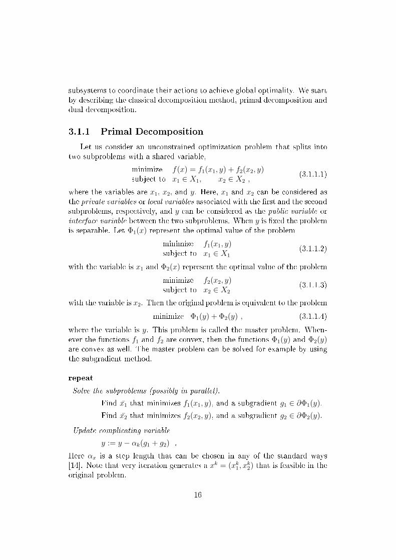
repeat

Solve the subproblems (possibly in parallel).

Find x1 that minimizes f1(x1, y), and a subgradient g1 ∈ ∂Φ1(y).

Find x2 that minimizes f2(x2, y), and a subgradient g2 ∈ ∂Φ2(y).

Update complicating variable

y := y − αk(g1 + g2) ,

Here αx is a step length that can be chosen in any of the standard ways[14]. Note that very iteration generates a xk = (xk1, x

k2) that is feasible in the

original problem.

16

3.1.2 Dual Decomposition

Let us next consider the same problem (3.1.1.1), but an equivalent formu-lation where we introduce new variables and enforce a consistency constrain,i.e.,

minimize f(x) = f1(x1, y1) + f2(x2, y2)subject to x1 ∈ X1, x2 ∈ X2

y1 = y2 ,(3.1.2.1)

where the variables are x1, x2, y1, and y2. Note that we have introduced a lo-cal version of the complicating variable y, along with a consistency constraintthat requires the two local versions to be equal. Note that the objective isnow separable, with the variable partition (x1, y1) and (x2, y2). Let us nowform the dual problem. The Lagrangian is given by

L(x1, y1, x2, y2, λ) = f1(x1, y1) + f2(x2, y2) + λTy1 − λTy2, (3.1.2.2)

and is separable. Let g1(λ) represent the optimal value of the problem

minimize f1(x1, y1) + λTy1subject to x1 ∈ X1

(3.1.2.3)

with the variable is (x1, y1) and g2(λ) represent the optimal value of theproblem

minimize f2(x2, y2) + λTy2subject to x2 ∈ X2

(3.1.2.4)

with the variable is (x2, y2). Then the dual function is given by

g(λ) = g1(λ) + g2(λ), (3.1.2.5)

where λ is the variable. Thus, the dual problem is expressed as

minimize g(λ) = g1(λ) + g2(λ) , (3.1.2.6)

with the variable is λ. This is indeed the master problem in dual decom-position. Again, we can use the subgradient method to solve the masterproblem (3.1.2.6) as follows:

17

repeat

Solve the subproblems (possibly in parallel).

Find x1 and y1 that minimizes f1(x1, y1) + λTy1.

Find x2 and y2 that minimizes f2(x2, y2) + λTy2.

Update dual variables

λ := λ− αk(y2 + y1).

Here αx is a step length that can be chosen in any of the standard ways [14].It is worth of noting that at each step of the dual decomposition algorithm, wehave a lower bound on p∗, the optimal value of problem (3.1.2.1). Speci�cally,we have

p∗ ≥ g(λ) = f1(x1, y1) + λTy1 + f2(x2, y2)− λTy2 , (3.1.2.7)

where x1, y1, x2, y2 are the subproblem (3.1.2.3)-(3.1.2.4) solutions during anyiteration of the subgradient method. The consistency constraint y1 = y2 isnot feasible in general, i.e., y2 − y1 6= 0. However, a feasible point can beconstructed from the iterate as

(x1, y), (x2, y) , (3.1.2.8)

where y = (y1 + y2)/2. As a result, an upper bound on p∗ is simply given by

p∗ ≤ f1(x1, y) + f1(x2, y). (3.1.2.9)

3.2 Alternating Direction Method of Multipli-

ers (ADMM)

The material presented in this section is based on [3], so we refer thereader to [3], for details. The main motivation for using ADMM is thatit combines the bene�ts of dual decomposition and augmented Lagrangianmethods for constrained optimizations. The result is a distributed algorithmwith fast (compared to the subgradient method) convergence properties. Westart with a simple convex constrained optimization problem. Then, wedescribe the dual ascent algorithm and augmented Lagrangian method forsolving this problem, which are the key ingredients for ADMM. Consider thefollowing convex constrained optimization problem

minimize f(x)subject to Ax = b ,

(3.2.0.10)

18

where the variable is x. The associated lagrangian is

L(x, y) = f(x) + yT (Ax− b) , (3.2.0.11)

where y is the dual variable or Lagrange multiplier associated with the equal-ity constraint. The dual problem is given by

maximize g(y) , (3.2.0.12)

where g(y) = infx L(x, y).In the dual ascent method, we solve the dual problem using gradient

ascent. Assuming that g is di�erentiable, the gradient ∇g of g at y is givenby

∇g(y) = Ax+ − b , (3.2.0.13)

wherex+ = arg min

xL(x, y) . (3.2.0.14)

Thus, the dual ascent algorithm is given by

xk+1 = arg minxL(x, yk) (3.2.0.15)

yk+1 = yk + αk(Axk+1 − b) , (3.2.0.16)

where αk is the step size. Note that (Axk+1−b) corresponds to the gradient ofg at yk, i.e., ∇g(yk). The �rst step is an x-minimization step, and the secondstep is a dual variable update. The dual variable y can be interpreted as avector of prices. This algorithm is called dual ascent since, with appropriatechoice of α, the dual function increases in each step.

However, in the case of convergence, the dual ascent algorithm discussedabove heavily relies on assumptions like strict convexity or �niteness of f[3]. Let us now describe the augmented lagrangian method, which gracefullyachieves convergence without such assumptions, and there more robust. Herewe consider the following equivalent problem formulation, instead of originalproblem (3.2.0.10)

minimize f(x) + (ρ/2)||Ax− b||22subject to Ax = b ,

(3.2.0.17)

where the variable is x and ρ is a positive scalar. We denote by Lρ(x, y) theLagrangian associated with problem (3.2.0.17), and is given by

Lρ(x, y) = f(x) + yT (Ax− b) + (ρ/2)||Ax− b||22 , (3.2.0.18)

19

where y represents the dual variables associated with the equality constraint.Applying dual ascent to the modi�ed problem (3.2.0.17) yields the algorithm:

xk+1 = arg minxLρ(x, y

k) (3.2.0.19)

yk+1 = yk + ρ(Axk+1 − b) , (3.2.0.20)

which is known as the method of multipliers. Note that the x-minimizationstep uses the augmented Lagrangian Lρ(x, y), instead of L(x, y) in (3.2.0.11).Moreover, the penalty parameter ρ is used in the place of αk in (3.2.0.16). Theconditions for convergence of the method of multipliers (3.2.0.19)-(3.2.0.20) isfar more general compared to the dual ascent method (3.2.0.15)-(3.2.0.16) [3].However, when f is separable, the augmented Lagrangian Lρ is not separable,because of the quadratic term ||Ax − b||22. As a result, the x-minimizationstep (3.2.0.19) cannot be performed in parallel for each subsystems.

We next describe the ADMM method, which can be considered as ablend between the dual ascent algorithm and the method of multipliers. Letus consider the problem of the form

minimize f(x) + g(z)subject to Ax+Bz = c ,

(3.2.0.21)

with variables x ∈ Rn and z ∈ Rm. The augmented Lagrangian for prob-lem (3.2.0.21) is given by

Lρ(x, z, y) = f(x)+g(z)+yT (Ax+Bz−c)+(ρ/2)||Ax+Bz−c||22 , (3.2.0.22)

where y denotes the dual variables as usual. Note that the direct applicationof method of multiplier method (3.2.0.19)-(3.2.0.20) for problem (3.2.0.21)results

(xk+1, zk+1) = arg minx,z

Lρ(x, z, yk) (3.2.0.23)

yk+1 = yk + ρk(Axk+1 +Bzk+1 − c) . (3.2.0.24)

In contrast, ADMM split the (x, z)-minimization step (3.2.0.23) into twosequential updates, namely x-minimization and z-minimization. Speci�cally,ADMM consist of the iteration

xk+1 = arg minxLρ(x, z

k, yk) (3.2.0.25)

zk+1 = arg minzLρ(x

k+1, z, yk) (3.2.0.26)

yk+1 = yk + ρ(Axk+1 +Bzk+1 − c) . (3.2.0.27)

20

where ρ is a positive scalar.There are many convergence results for ADMM in the literature. Here,

we do not go into explicit details and refer the reader for [3]. However, underthe assumptions 1) f and g are closed, proper, and convex, 2) the augmentedLagrangian has a saddle point, we list 3 interesting convergence propertiesof ADMM algorithm:

L0(x∗, z∗, y) < L0(x

∗, z∗, y∗) < L0(x, z, y∗) (3.2.0.28)

1. Iterates approach feasibility: Axk +Bzk − c→ 0 as k →∞ .

2. Objective function of the iterates approaches optimal valuef(xk) + g(zk)→ p∗ as k →∞, where p∗ is the optimal value .

3. Dual variable convergence. yk → y∗ as k → ∞, where y∗ is thedual optimal point .

rk+1 = Ak+1 +Bk+1 − c (3.2.0.29)

Compared to interior point algorithms, which are based on the Newton'smethod, the convergence of ADMM algorithm is noticeably slow. However,the convergence is faster compared to the dual ascent method or classicaldual decomposition techniques that rely on subgradient methods for solvingthe master problem.

3.3 Fast-Lispchitz optimization

An F-Lipschitz optimization problem is de�ned as:

maximize f0(x)subject to xi ≤ fi(x). i = i, ..., l

xi = hi(x), i = l + 1, . . . , n ,x ∈ D,

(3.3.0.30)

where D ∈ Rn is a non empty, convex and compact set, l ≤ n, with objectiveand constraints being continuous di�erentiable functions such that:

f0(x) : D → Rm, m ≥ 1

fi(x) : D → R, i = 1, ..., l

hi(x) : D → R, i = l + 1, ..., n

(3.3.0.31)

21

And the following three properties are satis�ed:

∇f0(x) ≥ 0 (f0(x)is strictly increasing, )

and

∇jfi(x) ≤ 0 ∀i 6= j, ∀x ∈ D∇jhi(x) ≤ 0 ∀i 6= j, ∀x ∈ D

or

∇if0(x) = ∇jf0(x) ∀i 6= j, ∀x ∈ D∇fi(x) ≥ 0 ∀i 6= j, ∀x ∈ D∇hi(x) ≥ 0 ∀i 6= j, ∀x ∈ D

and

|fi(x)− fi(y)| ≤ αi||x− y||, i = 1, ..., l ∀x, y ∈ D|hi(x)− hi(y)| ≤ αi||x− y||, i = l + 1, ..., n ∀x, y ∈ Dwith αi ∈ [0, 1), ∀i

(3.3.0.32)

All these properties are called, qualifying properties of an F-Lipschitzoptimization problem. The objective function and the constraints are allowedto be linear or non linear functions, as for instance concave, convex, mono-mial, polynomial, etc. and also decomposable or not. For an F-Lipschitzproblem is true the following theorem.

Theorem: Let an F-Lipschitz optimization problem be feasible. Then, theproblem admits a unique Pareto optimum x∗ ∈ D given by the solutions ofthe following set of equations:

x∗i = [fi(x∗)]D i = 1, ...l

x∗i = hi(x∗) i = l + 1, ..n

There is a unique optimal solution to F-Lipschitz optimization problems,which is achieved by solving the system of equations given by the projectedconstraints at the equality. If such a system of equations can be solved in aclosed form, then we have the optimal solution in a closed form, otherwise weneed numerical algorithms. The solution is obtained quickly by asynchronousalgorithms of certi�ed convergence. F-Lipschitz optimization can be appliedto both centralized and distributed optimization. Compared to traditionalLagrangian methods, which often converge linearly, the convergence time ofcentralized F-Lipschitz algorithms is superlinear. It is proved that a classof convex problems, including geometric programming problems, can be cast

22

as F-Lipschitz problems, and thus they can be solved much more e�cientlythan interior point methods. Some typical optimization problems that occuron wireless sensor networks are shown to be F-Lipschitz.

Distributed computationLet x(0) ∈ D be the initial value of the optimal solution to a feasible F-Lipschitz problem. Let xi(k) = [xi1(τ

i1(k)), xi2(τ

i2(k)), ..., xin(τ in(k))] the vector

of decision variables available at node i at time k ∈ N , where τ ij(k) is thedelay with which the decision variable of node j is communicated to nodei.Then, the following iterative algorithm converges to the optimal solution:

xi(k + 1) = [fi(xi(k))]D i = 1, ..., l (3.3.33)

xi(k + 1) = hi(xi(k)) i = l + 1, ..., n.

Every node i of the network collects asynchronously the decision variablesat timek and update its decision variable by the iteration (3.5.4). Noticethat when fi(x) depends only on the decision variables of the neighboringnodes, the communications of these variables to node i can be very fast. Inother situations, fi(x) can be given by an oracle locally at node i withoutany communication of decision variables from the other nodes. We refer thereader to [12] for details.

23

Chapter 4

Privacy preserving optimization

Privacy preserving problems are very common nowadays and the studyof more e�cient solutions is a topic more interesting. They occur in manyareas, such as data publishing, data mining, secret voting, auctions, scienti�cand statistical computations. The main requirements are that the entitiesinvolved in the system are unwilling to reveal the date they hold or makethem public and they may want to collaborate and �nd the solution of abigger problem without revealing the private data. A possible solution is forthe parties to agree on a commonly trusted entity T: then T could gatherthe private problem data, solve the optimization problem on behalf of theparties, and announce the result. Also, the parties can replace the trustedentity T with a cryptographic protocol while still preserving the same level ofsecurity that the trusted entity intuitively provides. These early protocols arehowever very far from being practical. There are some existing approachesto handle this kind of problem and a classi�cation of them is as follows:

• cryptographic methods;

• transformation-based methods;

• decomposition-based methods.

4.1 Privacy preserving solution methods

In this section we describe with more details the aforementioned ap-proaches.

Cryptographic methods use existing cryptographic techniques in orderto implement a privacy-preserving version of the Simplex or Interior Point

24

methods. The cryptography techniques are vary, like the secret sharing (eg.Shamir sharing) or thereshold homomorphic public key cryptography (eg.Pailler encryption). Also the homomorphic encryption and blind-and per-mute procedures to permute the tableau at each iteration, like in [15]. In [16]the authors used a solution approach based on secret sharing and the proto-cols use a variant of the simplex algorithm with �xed-point rational number,while in [17] the authors used a secret-sharing with shared matrix indexes.These techniques o�er better computational complexity give better perfor-mance over Simplex for very large problems [18], [19]. A privacy-preservinginterior point method has been presented in [26, chapter 8].

The transformation-based methods use some cryptography sub-protocolsin order to transform the original linear problem. The transformation of theproblem is made using random matrices and then the resulting problem issolved in the transformed domain. The cryptography sub-protocols are oftenused only at the beginning of the algorithm. Then, one party solved the trans-formed problem and the solution is converted back to the original problem.The �rst approach that used such transformation techniques was prosposedby Du [23] and now there are several improvements, expecially in terms ofthe level of the knowledge of the data of the interested parties. Bednarz [22],proposed a method, a modi�ed variants of the Du methods, where some ofthe complications of the original approach were removed. Bednarz consid-ers a case where the ownership of the objective function and the constraintsare distributed among two entities. Recently Mangasarian [4],[24] proposedthe �rst transformation method for the multi-party environments, where thedata are assumed to be vertically or horizontally partitioned. Here no cryp-tographic operations are required to apply the transformation, making thesemethods very e�cient compared to the methods relying on cryptography.

In decomposition-based methods the private data can be partitionedbetween the agents and they can collaborate to solve the problem in a par-allel and distributed fashion, without revealing their private variables. Theconcept of privacy is intrinsic. So each agent achieves its optimum usingonly local information. In this way the private data is not required to beexchanged among the agents to solve the problem and for that reason theyare privacy preserved. This falls in the general area of distributed decisionmaking with incomplete information.

The �rst two categories of methods are described in detail in [25]. Let usnext compare the three main approaches mentioned above.

25

4.2 Comparison of privacy preserving solution

methods

The �rst noticeable di�erence between cryptography and transformed-based methods is in their e�ciency of the computations. In cryptographicapproaches at each step of the algorithm the encryption/decryption of thedata is applied. In transformed-based methods, instead, these operationsof the private data are done only once. Therefore, transformed based ap-proaches can outperform cryptographic approaches, in terms of the computa-tional e�ciency. The decomposition techniques, however, do not require anykind of transformation domain because the data are inherently encrypted.This method is therefore much more e�cient than the others two. The sec-ond advantage is the freedom to use any LP solver, unlike the cryptographicmethod is tied to a particular LP solver. Another advantage of decomposi-tion techniques compared to the others two is that the methods are scalable.Therefore, very large problems can be handled gracefully by using decom-position techniques. Moreover, the decomposition techniques are fairly gen-eral and can address many places where the transformation based methodsfails. Most cryptographic methods, infact, is carried out over a �nite �eldand thus, is constrained to integer data values. For example, some of theSimplex-based methods impose integer restrictions on the objective functioncoe�cient and constraint coe�cients. This means that only integer vari-ants of Simplex can be used. Solving non trivial LP using these algorithmsleads to computations with integers potentially involving thousands of bits.Therefore, cryptographic approaches are not good in the case of large prob-lems. Transformation-based methods and decomposition based approaches,instead, are free to use �oating-point arithmetics. Finally, the algorithms areconceptually simpler, good for large problems and don't require specializedoptimization software.

Transformed-based methods and decomposition based approaches have,however, several disadvantages compared to the cryptographic methods. Themost important one is that these methods only provide heuristic securityguarantees, Indeed, without the cryptographic protocols at each step, se-curity is more challenging to prove. Cryptographic approaches guarantee arobust security. Another limit of transformation-based methods and the de-composition based approaches is the dependence to the problem structure, inparticular on the way the data is partitioned between agents. There is alsono standard way to de�ne the subset of LPs to which a transformation ap-plies. The cryptographic methods, instead, are more generics and robust toproblem structure and the types of contraints and variables. In the table 4.1

26

Cryptographicmethods

Transformation-based methods

Decomposition-based methods

ine�cient e�cient e�cientrestricted to LP prob-lem

not restricted to LPproblem

not restricted to LPproblem

protocols often tied toa particular solver

free to use any solver free to use any solver

operations are re-stricted to �nite �eld

handle real/complexvecor spaces

handle real/complexvecor spaces

small scale problems large scale problems very large scale prob-lems

not scalable scalable scalableprivacy via encrypteddomain

privacy via trans-formed domain

privacy is intrinsic

robust to problemstructure

very sensitive to prob-lem structure

data partitioning de-pendence

robust security guaran-tees

heuristic security guar-antees

heuristic security guar-antees

Table 4.1: Privacy preserving classi�cation based on the classical distributedoptimization methods

we summarize main advantages and disadvantages that we discussed above.

4.3 Privacy preserving classi�cation problems

In this section we categorize some existing methods to solve decentral-ized optimization problem in terms of privacy preserving. In particular wecategorize these methods based on the di�erent level of privacy preservingrequest in the problem. Also, there are several kind of optimization prob-lems, such linear, convex, non conex and Fast-Lipschitz. So, depending onthe mathematical nature of the problem, we try to �nd a speci�c algorithmthat solve it in the better way. Distributed optimization is used in a widearea of problems, such as Cloud Computing, Data Mining, Vehicular Rount-ing, Online Learning, Belief Propagation, Destributed Estimation and so on.So, another classi�cation is based just on the kind of the application.

27

4.3.1 Privacy preserving algorithms

A particular privacy preserving method applied to a linear optimiza-tion problem are described in [4]. This approach will allow us to solvea distributed optimization problem by a random linear transformation thatwill not reveal any of the privately held data but will give a publicly availableexact minimum value to the origianl problem. Thus, we are able to solve aprivacy preserving transformed linear program that generates an exact so-lution to the original linear program without revealing any of the privatelydata of which node. The m-by-n constraits matrix A of the bacis linear prob-lem is divided into p blocks of columns, each block of which toghether withthe corresponding block of cost vector, is owned by a distinct entity. Eachentity not willing to share or make public its column group or cost coe�cientvector. Component groups of the solution vector of the privacy preservingtransformed linear program can be decoded only by the group owners andcan be made public by these entities to give the exact solution vector of theoriginal linear problem.

Considering the problem of optimizing a convex function subject toa collection of convex inequality constraints and set constraints, we could re-fer to the paper [5]. In which is assumed that each node has a set of a privateoptimization variables that partecipate in the global optimization problembut are unknown to other nodes of the graph. This distributed algorithmoperates over any connected graph of processors and yields a solution that isarbitrarily close to a global optimal solution, where proximity to optimalityis controlled by a parameter that a�ects a tradeo� in the required computa-tion time. This new algorithm is inspired of Lyapunov drift theory.

In [11] is proposed a new distributed algorithm, namedD-ADMM, basedon the alternating direction method of multipliers (ADMM) for solving. Ina separale optimization problem, the cost function, and the constraint setis the intersection of all the agents' private constraint sets. In this paperis required the private cost function and the constraint set of a node to beknown by that node only, during and before the execution of the algorithm.

If we have an optimization problem with a concave objective func-tion we could refer to [6]. The paper proposes an adaptation of Lagrangianmethod to solve distributed weighting method for both strictly concave andnot strictly concave (e.g. linear) value functions for a maximization problem,maintaining the privacy of the participating parties.

28

In Cloud Computing the concept of privacy preserving has an impor-tant role. Indeed, costumer con�dential data processed and generated dur-ing the computation need to be secret. The problem of securely outsourcingcomputation in cloud computing is formalized in [7]. It is based on on aproblem transformation techniques that enable customers to secretly trans-form the original problem into some random one while protecting sensitiveinput/output information.

Another �eld in which privacy preserving plays an important role is On-line Learning. In [8] is considered a general distributed outonomous onlinelearning algorithm to learn from fully decentralized data sources. Learnersneed to exchange information between them, so a local learner updates itslocal parameter basing on the local subgradient and then propagates the pa-rameter to other learners. The paper examines under which conditions amalicious node cannot recostruct all subgradients of other nodes based onthe parameter vectors of its adjacent nodes. So, the algorithm has intrinsicprivacy preserving properties if the network topologies respect some condi-tions.

Belief propagation, also known as Sum-product message passing, is amessage passing algorithm for performing inference on graphical models, suchas Bayesian networks and Markov random �elds. It calculates the marginaldistribution for each unobserved node, conditional on any observed nodes.Belief propagation is commonly used in arti�cial intelligence and informationtheory and has demonstrated empirical success in numerous applications in-cluding low-density parity-check codes, turbo codes, free energy approxima-tion, and satis�ability. The paper [9] provides provably privacy preservingversions of belief propagation and other local message passing algorithms onlarge distributed networks. Each party learns their conditional probability ofexposure to the didease and absolutely nothing else. A party can e�cientlycompute after having partecipated in the protocol, they could have e�cientlycomputed alone given only the value of their conditional propability. Thus,the protocol leaked no additional information beyond its desired outputs.The paper shows how to blend tools from cryptography with local messagepassing algorithms in a way that preserves the original computations, but inwhich all messages appear to be randomly distributed from the viewpoint ofany individual.

TheVehicle Routing Problem (VRP) is a combinatorial optimizationand integer programming problem seeking to service a number of customerswith a �eet of vehicles. In its multiple depot variant, the routes of vehicles

29

Distributedsolver method

Privacy pre-serving deci-sion variables

Privacy pre-serving utilityfunction

Privacy pre-serving con-straints

Primal Decom-position

√| |

Dual Decompo-sition

√| |

ADMM|

√|

Fast-Lipschitz|

√ √

Table 4.2: Privacy preserving classi�cation based on the classical distributedoptimization methods

located at various depots must be optimized to serve a number of costomers.The paper [10] investigates how to protect the privacy of delivery companies,when each depot is owned by a di�erent company with a limited view of theoverall problem.

4.3.2 Classi�cation based on the classical distributed

optimization methods

In the �rst chapter we discussed the most important methods to solve adistributed optimization problem. Now, we categorize these methods by theviewpoint of privacy preserving. So, in the table 4.2 we explain, for each ofthem, if it is privacy preserving in terms of utility function, decision variablesor contraints.

30

Mathematicalnature

Privacy preserv-ing decision vari-ables

Privacy preserv-ing utility func-tion

Privacy preserv-ing constraints

Linear [4] [4] [4]Convex

|[5],[11] [5],[11]

Non Convex|

[6]|

Fast-Lipschitz|

[12] [12]

Table 4.3: Privacy preserving classi�cation based on the mathematical natureof the optimization problem

4.3.3 Classi�cation based on the mathematical nature

of the optimization problem

Another kind of classi�cation is based on the mathematical nature of theoptimization problem. As view in the previous chapter, there are some pa-pers which propose a method to solve each of them. In particular we canmake a classi�cation to linear, convex, non convex and F-Lipshitz problem.For each entry of the table we indicate which paper solve the problem, alwaysmaking a distinction about the level of privacy preserving they approach (seetable 4.3).

4.3.4 Classi�cation based on the application

In the previous chapter we talked about various application based on dis-tributed optimization that require privacy preserving. So, in the table (4.4)we make a classi�cation of them.

31

Application Privacy preserv-ing decision vari-ables

Privacy preserv-ing utility func-tion

Privacy preserv-ing constraints

Online Learning [8] [8]|

Cloud Comput-ing

[7] [7] [7]

Belief Propaga-tion

[9] [9] [9]

Vehicle Routing [10]| |

Table 4.4: Privacy preserving classi�cation based on the application

32

Chapter 5

Car-parking problem

One of the most relevant problem in urban transportation is the tra�ccongestion and parking di�culties, which are also a major cause for losingtime. These two problems are interrelated since looking for a parking spacecreates additional delays and impairs local circulations. Given the impor-tance of e�cient car parking strategies, in this chapter, we place a greateremphasis on car parking problem, together with privacy preserving proper-ties. Our goal is to reduce the distance from the parking slot to the intendeddestination of the car, thus helping the driver to easily �nd a parking closerto their places of interest.

Our proposed solution method is privacy preserving, in the followingsense: vehicles do not want to reveal their destinations during the algorithmiterations. In addition, the proposed solution method is distributed amongusers (vehicles) with a little central coordination. Moreover, the method isfair, roughly speaking, it �nds a allocation such that the maximum distanceto from the parking slot to the destination of cars is minimized. Thus, oursolution method is privacy preserving distributed, and fair.

In particular, we consider the car park illustrated in the �gure 5.1 tomathematically model the problem. Parking slot assignment is time slotted,with slot period T . At the beginning of any time slot t, the number of freeslots in the park should be known. Moreover, their details (e.g., locationinformation) should be informed to the selected set of cars which are sched-uled for parking at the beginning of the time slot t. Each car then knowsthe distances from free slots to their intended destination. In particular, thisinformation is simply extracted from a table (see table 5.2), which containsall the distances from every free slot to every shop. At the beginning of timeslot t, it is required to decide the slot-vehicle assignment, which is indeed thebinary decision variables. This is shown in table 5.3. For example, if the j-thslot is occupied by the i-th vehicle, we indicate this assignment by using 1 in

33

aij di

Sj

Figure 5.1: Car-Parking model

the (ij)th position, otherwise 0. The formulation can model parking assign-ments for di�erent kind of vehicles, with di�erent sizes and dimensions, e.g.,cars, vans, motorbikes, and scooters.

In such a formulation, vehicles should maintain data such as the dimen-sion of the slots. Roughly speaking, the following should be considered inthe problem formulation.

• The distances from free slots to the destinations or shops. This informa-tion is required for constructing the objective function of the problem.

• The availability of the slots and their assignment: this is required forexpressing constraints to enforce a correct assignment. For example,the assignment shown in table 5.3 is correct. But the assignment shownin table 5.4 is incorrect.

• The dimensions of the vehicles over the slots: this information is againrequired for expressing constraints.

34

Shops Slots

S1 S2 S3 S4 S5

shop1 a11 a12 a13 a14 a15shop2 a21 a22 a23 a24 a25shop3 a31 a32 a33 a34 a35shop4 a41 a42 a43 a44 a45

Table 5.1: Table of distances: for each shop (vehicle destination) is indicatedthe distance to each slot of the parking.

Shops Slots

S1 S2 S3 S4 S5

shop1 a11 a12 a13 a14 a15shop2 a21 a22 a23 a24 a25shop3 a31 a32 a33 a34 a35shop4 a41 a42 a43 a44 a45

Table 5.2: Table of distances: for each shop (vehicle destination) is indicatedthe distance to each slot of the parking.

Vehicles Slots

S1 S2 S3 S4 S5

vehicle1 0 0 1 0 0vehicle2 0 0 0 0 1vehicle3 1 0 0 0 0vehicle4 0 0 0 1 0

Table 5.3: Table of slots' availability: for eache slot is indicated if it's assignedto some vehicles or not.

Vehicles Slots

S1 S2 S3 S4 S5

vehicle1 0 0 1 0 0vehicle2 0 0 0 0 1vehicle3 1 0 0 0 0vehicle4 1 0 0 1 0

Table 5.4: Incorrect assignment of parking

35

5.1 Notations

Now we introduce essential notations to formulate the problem:

• j = 1, ...,M : the indexes of the parking slots

• Wj: the width of jth slot

• Lj: the length of jth slot

• i = 1, ..., N : the indexes of the scheduled vehicles for parking at thebeginning of the time slot

• wi: the width of ith vehicle

• li: the length of ith vehicle

• di = (dxi , dyi ): the destination coordinates of the ith vehicle

• aij(di): the distance from the jth slot to the destination of ith vehicle.In particular, let (sxj , s

yj ) denote the coordinates of the jth slot. Then,

aij(di) is given by

aij(di) = α√

(dyi − syj )

2 + (dxi − sxj )2 ,

where α is a parameter known to all the scheduled vehicles only andis used to perform a scalar transformation to the distance. This scalartransformation further increases the privacy of the destinations of thevehicles to a third party.

• xij: the variable to indicate the vehicle-slot assignment. In particular,

xij =

{1 if the jth slot is assigned to the ith vehicle0 otherwise

(5.1.1)

36

5.2 Problem formulation

The car-parking problem explained in the previous chapter can be writtenin a mathematical form as follow:

minimize maxi∈N

M∑j=1

xijaij(di)

subject toN∑i=1

xij ≤ 1, ∀j (5.2.0.1)

M∑j=1

xij = 1, ∀i (5.2.0.2)

xij ∈ {0, 1} (5.2.0.3)

Wj ≥ wixij, ∀i, j (5.2.0.4)

Lj ≥ lixij, ∀i, j (5.2.0.5)

where the variables are xij, i = 1, . . . , N , j = 1, . . . ,M . The constraint(5.2.0.1) requires that each slot is assigned at most to one vehicle. Such anassignment is shown in table 5.3, where parking slots S2 has been assignedno vehicles and all others have been assign one vehicle each. Table 5.4 showsa constraint violation, where two vehicles (vehicle3 and vehicle4) have beenassigned the same slot (i.e., the parking slot S1). Constraint (5.2.0.2) im-poses the condition that each vehicle must be assigned to a slot. In thisthesis we assume that the number of scheduled vehicles is smaller than thefree parking slots, i.e., N ≤ M . Otherwise the problem is clearly infeasible.Thus, a schedular should take into account these issues, which are extraneousto the main focus of the thesis. See table 5.3 and table 5.4 for examples ofcorrect and incorrect assignments, respectively. Constraint (5.2.0.3) requiresthat the values of xij to be 0 or 1.

Constraints (5.2.0.4-5.2.0.5) are clearly associated with dimensions of slotsand vehicles (see �gure 5.2 and 5.3). For notational simplicity, let

βij =Wj

wi

and

γij =Ljli.

37

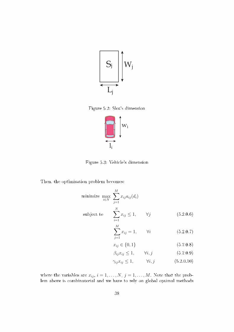
Wj

Lj

Sj

Figure 5.2: Slot's dimension

wi

li

Figure 5.3: Vehicle's dimension

Then, the optimization problem becomes:

minimize maxi∈N

M∑j=1

xijaij(di)

subject toN∑i=1

xij ≤ 1, ∀j (5.2.0.6)

M∑j=1

xij = 1, ∀i (5.2.0.7)

xij ∈ {0, 1} (5.2.0.8)

βijxij ≤ 1, ∀i, j (5.2.0.9)

γijxij ≤ 1, ∀i, j (5.2.0.10)

where the variables are xij, i = 1, . . . , N , j = 1, . . . ,M . Note that the prob-lem above is combinatorial and we have to rely on global optimal methods

38

such as exhaustive search and branch and bound methods to solve it. Themain disadvantage of global methods is the prohibitively expensive compu-tational complexity, even in the case of very small problems. Such methodsare not scalable and impractical. In the sequel, we provide a method basedon duality. Even though the optimality cannot be guaranteed, the proposedmethod is e�cient, fast, and allows distributed implementation with a littlecoordination from a central controller. Therefore, the method is favorablefor practical implementations.

5.3 Finding the dual problem

We start by equivalently formulating problem (5.2.0.6-5.2.0.10) in its epi-graph form. The equivalent problem is given by

minimize t

subject toM∑j=1

xijaij(di) ≤ t, ∀i (5.3.0.1)

N∑i=1

xij ≤ 1, ∀j (5.3.0.2)

M∑j=1

xij = 1, ∀i (5.3.0.3)

xij ∈ {0, 1} (5.3.0.4)

where the variables are t and x = (xij)i=1,...,N,j=1,...,M . Note that we have re-moved the constraints (5.2.0.9-5.2.0.10) of the original problem for simplicity.But the solution method to be given fully extends to include the constraints(5.2.0.9-5.2.0.10) as well. Now we want to apply duality theory to the epi-graph form. It is important to note that we want also to decouple the problemamong the vehicles. We can clearly see that constraints (5.3.0.1-5.3.0.2) arethe coupling constraints of the problem. The constraints (5.3.0.3-5.3.0.4)are already decoupled among the vehicles and we can treat them as implicitconstraints. Next, we introduce Lagrange multiplies and form the partialLagrangian by dualizing the coupling constraints (5.3.0.1-5.3.0.2). So, wehave to introduce the Lagrangian multipliers, in particular λ = (λi)i∈{1,...,N}for the �rst set of inequality constraints and multipliers µ = (µj)j∈{1,...,M}

39

for the second set of inequality constraints. The Lagrangian associated withproblem (5.3.0.1-5.3.0.4) is:

L(t, x, λ, µ) = t+N∑i=1

λi(M∑j=1

xijaij(di)− t) +M∑j=1

µj(N∑i=1

xij − 1)

= t+N∑i=1

M∑j=1

λixijaij(di)−N∑i=1

λit+M∑j=1

N∑i=1

µjxij −M∑j=1

µj

= t(1−N∑i=1

λi) +N∑i=1

M∑j=1

(λiaij(di) + µj)xij −M∑j=1

µj

(5.3.0.5)

Now we need to �nd the dual function g(λ, µ). To do this, we minimizethe Lagrangian with respect to primal variables t and x, i.e.,

g(λ, µ) = inft∈R,∑M

j=1 xij=1,∀i,xij∈{0,1},∀i,j

L(t, x, λ, µ)(5.3.0.6)

=

inf∑M

j=1 xij=1,∀i,xij∈{0,1},∀i,j

∑Ni=1

∑Mj=1(λiaij(di) + µj)xij −

∑Mj=1 µj

∑Ni=1 λi = 1

−∞ otherwise(5.3.0.7)

=

∑N

i=1(inf∑Mj=1 xij=1,∀i,

xij∈{0,1},∀i,j

∑Mj=1(λiaij(di) + µj)xij)−

∑Mj=1 µj

∑Ni=1 λi = 1

−∞ otherwise(5.3.0.8)

=

∑N

i=1 gi(λ, µ)−∑M

j=1 µj∑N

i=1 λi = 1

−∞ otherwise

(5.3.0.9)

40

In 5.3.0.7, we have removed the linear term

t(1−N∑i=1

λi) ,

because it is bounded below only when∑N

i=1 λi = 1. The constraints of infoperator in 5.3.0.7 are separable among the vehicles i ∈ {1, . . . , N}. There-fore, we can move the inf operator inside the summation

∑Ni=1, see (5.3.0.8).

The function gi(λ, µ) denotes the optimal value of the following problem:

minimizeM∑j=1

(λiaij(di) + µj)xij

subject toM∑j=1

xij = 1,

xij ∈ {0, 1} ,∀j,

(5.3.10)

with the variable (xij)j∈{1,...,M}. Each vehicle has to solve the problem (5.3.10).Note that the problem (5.3.10) is combinatorial, but it has a closed form so-lution given by:

x∗ij =

1 j = arg minn∈{1,...,M}(λiain(di) + µn)

0 otherwise(5.3.11)

The dual problem is given by:

maximize g(λ, µ) =N∑i=1

gi(λ, µ)−M∑j=1

µj

subject toN∑i=1

λi = 1,

λi ≥ 0, ∀i,

µj ≥ 0,∀j .

(5.3.12)

where variables are (λi)i∈{1,...,N} and (µj)j∈{1,...,M}.

41

5.4 Solving the dual problem

To solve the dual problem 5.3.12 we use the projected subgradient method,which is often applied to large-scale problems with decomposition structures.Note that g(λ, µ) is a concave function, therefore, we need to �nd the sub-gradient of −g at a feasible (λ, µ). We denote by s the subgradient and forclarity we separate s into two vectors as follows:

s = (u, v), (5.4.0.1)

where u = (ui)i∈{1,...,N} is the part that corresponds to λ and v = (vj)j∈{1,...,M}the part that corresponds to µ. The (negative of) dual function −g(λ, µ) isgiven by

− g(λ, µ) =M∑j=1

µj −N∑i=1

gi(λ, µ)

=M∑j=1

µj −N∑i=1

M∑j=1

(λiaij(di) + µj)x∗ij

=M∑j=1

µj −M∑j=1

µj

N∑i=1

x∗ij −N∑i=1

λi

M∑j=1

aij(di)x∗ij.

So we obtain, for all i ∈ N :

ui = −M∑j=1

aij(di)x∗ij and vj = 1−

N∑i=1

x∗ij, (5.4.0.2)

where x∗ij given in (5.3.11). The projected subgradient method is given by

(λ, µ)(k+1) = P ((λ, µ)(k) − αk(u, v)(k)), (5.4.0.3)

where k is the current iteration index of the subgradient method, P (z) de-notes the Euclidean projection of z onto the feasible set of the dual problem(5.3.12), and αk > 0 is the kth step size, chosen to guarantee the asymptoticconvergence of the subgradient method, e.g., αk = 1/k. Since the feasible setof dual problem is separable in λ and µ, the projection P (·) can be performedindependently. Therefore, the iteration (5.4.0.3) is equivalently performed asfollows:

λ(k+1) = Ps(λ(k) − αku(k)) (5.4.0.4)

µ(k+1) = [µ(k) − αkv(k)]+, (5.4.0.5)

42

where Ps(·) is the Euclidean projection onto the probability simplex{λ∣∣∣∑N

i=1 λi = 1, λi ≥ 0}

and [ · ]+ is the Euclidean projection onto the nonnegative orthant.

5.5 Distributed implementation

Let us now present the distributed solution methods for the car park-ing problem. Here, we capitalize on the ability to construct the subgradient(u, v) in a distributed fashion via the coordination of scheduled vehicles. Aswe have already mentioned, there should be a little involvement of a centralcontroller (e.g., owner of the car park) for realizing the overall algorithm.This involvement is mainly for dual variable updating and broadcasting newdual variables to the scheduled vehicles until the algorithm stops.

Algorithm : Distributed algorithm for car-parking

1. Central controller sets k = 1 and broadcasts the initial (feasible) λ(k)i

and (µ(k)j )j=∈{1,...,M} to vehicle i, i ∈ {1, . . . , N}.

2. Vehicle i sets λi = λ(k)i and µ = µ(k) and locally solves the problem

(5.3.10), to yield the solution (x∗ij)j=1,...,M , which is given by (5.3.11).

3. Vehicle i computes scalar ui from (5.4.0.2) and transmits this to thecentral controller. For each j, scheduled vehicles communicate (binaryvariables x∗ij) and construct the scalar vj and transmits this to thecentral controller.

4. Subgradient iteration:

• Central controller forms u(k) and performs (5.4.0.4)

• Central controller forms v(k) and performs (5.4.0.5).

5. Stopping criterion: if the stopping criterion is satis�ed, then STOP.Otherwise, set k = k + 1, and central controller broadcasts the newλ(k)i , (µ

(k)j )j∈{1,...,M} to vehicle i, i = 1, . . . , N , and go to step 2.

43

5.5.1 Algorithm description

In step 1, the algorithm starts by choosing initial feasible values forλ(k)i , i = 1, . . . , N and µ

(k)j , j = 1, . . . ,M . After receiving these values from

the central controller, each vehicle computes both {xij}j∈{1,...,M} in step 2 ina decentralized fashion. Step 3 is used for communication and coordination.In particular, each vehicle i constructs scalar parameter ui and sends this tothe central controller. Moreover, scheduled vehicles communicate binary pa-rameters to construct vj and transmits this to the central controller. We seethat the solution method is privacy preserving, because no one (vehicles andthe central controller) can guess vehicle i's destination data (dxi , d

yi ). Note

that, step 3 does not reveal the private destinations of vehicle i, i.e., (dxi , dyi )

to the the central controller. This is mainly because, (dxi , dyi ) is hidden inside

ui. However, for larger iteration index k, the central controller can guess thatthe algorithm has a feasible solution and as a result, −ui = aij(di) for someparking slot j. But, still aij(di) is a α-scaled version of the true distancefrom vehicle i's parking slot to its intended destination. Therefore, with-out knowing α, the central controller �nds it di�cult to compute vehicle i'strue destination coordinates (dxi , d

yi ). Moreover, in step 3, the scheduled

vehicles coordinate their solutions (xij)j∈{1,...,M} with each other. This com-munication also privacy preserving, because, no scheduled vehicle can knowthe vehicle i's problem data (aij(di))j∈{1,...,M}. Then, the algorithm performstep 4, the subgradient iterations (5.4.0.4-5.4.0.5). In this way it generates a

sequence of λ(k)i and µ

(k)j , k = 1, . . .. The price update or the Lagrange mul-

tiplier update mechanism attempt to achieve primal feasibility of the originalproblem (5.3.0.1-5.3.0.4). However, because the problem is nonconvex, pri-mal feasibility is often not guaranteed. Therefore, it usually required to calla subroutine to construct a feasible solution at the end of the algorithm.

Finally, step 5 is the stopping criteria. If it is satis�ed, then the algorithmstops, otherwise central controller broadcasts λ

(k)i and µ(k) to all vehicles

i ∈ {1, ..., N} and the algorithm is repeated.

5.5.2 Recovering the primal feasible point

By using the algorithm above, we �nd the optimal dual variables. Butthe main requirement is to �nd an optimal solution for the primal problem.However, this is often impossible. First, note that the problem is nonconvexand as a result there is no guarantee that dual approach that we followedgives a mechanism for �nding the optimal primal solution or even a primalfeasible point. Therefore, as pointed in the description of step 4, we have torely on a (heuristic) subroutine to construct a primal feasible point after the

44

algorithm terminates. In this thesis, we do not discuss such issues.

45

Chapter 6

Numerical results

In this chapter, we show simulation results to see the behavior of ourproposed algorithm. Simulations were run with the MATLAB environmentand carried out on a 3,4 GHz, Intel Core i7-2600 personal computer.

At the beginning of every time slot t ∈ {1, . . . , T}, the total number ofscheduled vehicles is assumed to be �xed, which is denoted by N and thetotal number of free parking slots is assumed to be �xed, which is denotedbyM . Of course, the algorithm is not restricted to �xed scenarios. Fixing Nand M as mentioned above is useful to see the key behaviors of the proposedmethod. At the beginning of every time slot t, the α-scaled distances aij(di),i = 1, . . . , N , j = 1, . . . ,M were randomly generated. Note that α hereis an arbitrary scalar known to the scheduled vehicles only. Without loss ofgenerality, we let α = 1 in all the simulations. In each time slot, the proposedalgorithm is carried out for K = 300 subgradient iterations. Moreover, weaverage over T = 1000 time slots to obtain average performances of thealgorithm. Finally and most importantly, for every t ∈ {1, . . . , T}, we keeptrack of the best point found so far by the algorithm during its subgradientiterations k = 1, . . . , K. We denote by x(t, k) the best point and by p(t, k)the corresponding overall objective value (i.e., the primal objective value ofproblem (5.3.0.1-5.3.0.4)) in time slot t and in subgradient iteration k. Recallfrom section 5.5.2 that, we do not use any subroutines to construct a primalfeasible point at the end of the proposed algorithm. As a result, of course,the best point x(t, k) found so far can be infeasible to the original primalproblem (5.3.0.1-5.3.0.4). Therefore, if a primal feasible point is not attainedby the algorithm in time slot t and in subgradient iteration k, then we setthe corresponding p(t, k) =∞.

46

0 5 10 15 200

10

20

30

40

50

60

70

80

90

100

Users

Fea

sibi

lity

Figure 6.1: Feasibility versus vehicles or users; �xed number of parking slots,i.e., M = 20

6.1 Feasibility of the proposed method

First we show results relating to the solution's feasibility. In particular,we de�ne a percentage measure of feasibility as follows:

Feasibility =

∑Tt=1 I(p(t,K) <∞)

T× 100 % , (6.1.0.1)

where I(E) is the indicator function of event E and recall thatK = 300 is thetotal subgradient iterations and T = 1000 is the total time slots considered.

Figure 6.1 illustrates the change in the feasibility for �xed number ofparking slots (i.e., M = 20) as the number of users N is increased from 3 to20. The behavior is intuitively expected, because we have not implementedany subroutine to construct a feasible point at the end of the algorithm.However, results show that for all N ≤ 10, the algorithm often �nds a feasiblepoint, even without such subroutines.

Figure 6.2 shows the change in feasibility for �xed number of users (i.e.,N = 3) as the number of parking slots M is increased from 3 to 20. Resultsagree with out intuition: as the number of free slots increases, the feasibilityincreases.

47

0 5 10 15 2094

95

96

97

98

99

100

Slots

Fea

sibi

lity

Figure 6.2: Feasibility versus parking slots; �xed number of vehicles or users,i.e., N = 3

Roughly speaking, the results in �gure 6.1 and �gure 6.2 indicate thatas long as N ≤ (M/2), our proposed algorithm very likely returns a feasiblepoint. Therefore, to further investigate the behavior of the proposed algo-rithm, in the following experiments, we stick toN andM values as mentionedabove. As we already mentioned, when the resulting point is infeasible, wemust rely on a subroutine to construct a primal feasible point. During thisthesis those issues are not considered and are left for future research.

6.2 Comparison with other benchmarks

For evaluating the performance of our algorithm we compare it with thefollowing benchmarks:

• Random method: This method employs a random parking slot as-signment to each vehicle.

• Greedy method: This method employs a greedy parking slot assign-ment as follows. First, the vehicles are ordered. The �rst vehicle inthe top of the order chooses its optimal parking, i.e., the parking slot

48

50 100 150 200 250 30085

86

87

88

89

90

91

92

93

Subgradient iterations

Obj

ectiv

e va

lue

greedyproposed methodexhaustive

Figure 6.3: Average objective value p(k) versus subgradient iterations k;N = 3 and M = 20.

closest to its destination. Then the next vehicle in the order looks in tothe remaining free parking slots and selects the best one for him. Themethod continues until all scheduled vehicles have there own parkingslots.

• Exhaustive method: This method computes all the combinationsand �nds the optimal parking slot assignment.

For comparison, we �rst consider the following performance metric:

p(k) =∑T

t=1 p(t, k), k = 1, . . . , K = 300 . (6.2.0.1)

The metric p(k) is a measure of the average objective value at subgradientiteration k.

Figure 6.3 shows the average objective value p(k) of our proposed methodversus the subgradient iteration k. Results are plotted for N = 3 andM = 20. For comparison, we have also plotted the average objective val-ues obtained by benchmark algorithms. Note that the benchmark plots arestraight lines, because they do not have subgradient iterations as our pro-posed method. Results show that the performance gap between our proposedmethod and the optimal exhaustive method become almost zero for larger

49

50 100 150 200 250 300112

114

116

118

120

122

124

126


Obj

ectiv

e va

lue



subgradient iterations k. For example, see p(k) for k ≥ 200. Results fur-ther show that our method outperforms both the greedy and the randommethod 1

Figure 6.4, 6.5, and 6.6 show again the average objective value p(k) ofour proposed method versus the subgradient iteration k for cases 1) N = 3and M = 15, 2) N = 3 and M = 10, and 3) N = 3 and M = 5, respectively.Benchmark curves are plotted for comparisons. Note that there are somemissing parts of the curves corresponds to our algorithm, see �gure 6.5 and6.6. For example, in the case of �gure 6.5, curve that corresponds to ourmethod starts at k = 50. This behavior is due to the primal infeasibility:i.e., for all k ≤ 50, the point x(t, k) is infeasible for some time slot t ∈{1, . . . , T = 1000}. As a result, p(k) = ∞ for all k ≤ 50 and not plotted inthe �gure. The performances in all considered cases are very similar to thosediscussed in the case of Figure 6.3. Our algorithm achieves almost optimalvalue for large values of k. Moreover, after some subgradient iterations, ourproposed method outperforms both the greedy and the random methods.

1Curve that corresponds to the random method is excluded from the �gure for clarity

beacause the average objective value given by the random method is too high.

50

50 100 150 200 250 300162

164

166

168

170

172

174

176

178


Obj

ectiv

e va

lue



Next, we de�ne the following performance metric:

Deviation with respect to optimal method (Dopt) =X − p∗

p∗× 100 % ,

(6.2.0.2)where p∗ is the optimal objective value obtained from the exhaustive methodand X can be either the average objective value obtained from the randommethod, the greedy method, or our proposed method. In particular, we letX = p(K) for our method.

In tables 6.1, 6.2 and 6.3 we illustrate the exact values of the objectivefunction in random, greedy and proposed methods and also the deviationvalue from the Dopt.

In particular, table 6.1 shows the performance comparisons of di�erentalgorithms for the case N = 3 and M = 20. We have tabulated the themetric Dopt de�ned above together with the associated suboptimal objec-tive values of random, greedy, and proposed methods. We can see that theobjective value of the random method is too high, with a deviation Dopt of777, 14%. The greedy method, instead, has an acceptable objective value,with a deviation Dopt of 3, 14%. But proposed method outperforms bothmethods above, infact its deviation from the optimal is zero.

51

50 100 150 200 250 300320

322

324

326

328

330

332


Obj

ectiv

e va

lue


Figure 6.6: Average objective p(k) versus subgradient iterations k; N = 3and M = 5.

Method AVG of Objectivefunction

Deviation from op-timal (%)

Random 750, 5491 777, 14%

Greedy 88, 2119 3, 14%

Proposed 85, 5397 ∼= 0%

Table 6.1: Achieved objective value and deviation Dopt; N = 3 and M = 20

52


Deviation from op-timal (%)

Random 838, 2 682, 6%

Greedy 117, 2 9, 5%

Proposed 108, 1 0, 9%

Table 6.2: Achieved objective value and deviation Dopt; N = 5 and M = 20

Table 6.2 shows again the objective value and performance metric Dopt

comparisons for the case N = 5 and M = 20. The results are very similar tothose observed in table 6.1. We can note that the deviation of the randommethod is still unacceptable. The deviation of the greedy method has alsobeen increased substantially from 3.14% to 9.5%. However, interestingly, thechange in deviation of our proposed method is very small.

Now we consider a larger dimensional problems in which the exhaustivemethod is not applicable. So we consider a new deviation metric, Dnon−opt,de�ned as:

Deviation with respect to proposed method (Dnon−opt) =X − p(k)

p(k)×100 % ,

(6.2.0.3)where p(K) is the average objective value from our proposed method afterK=300 subgradient iterations andX can be either the average objective valueobtained from the random method or the greedy method.

Table 6.3 shows the objective value and performance metric Dnon−optcomparisons for a larger dimensional problem. In particular, we consider acase with N = 10 and M = 20. The objective value of the random methodis again unacceptable, with a deviation of 539, 3%. Also, we can see that thedeviation of the greedy method increases substantially, 26, 32%.

6.3 CPU time comparison

Now we compare the CPU time performances of proposed method com-pared to the exhaustive method. Note that proposed method uses K = 300

53


Deviation from pro-posed method's op-timum (%)

Random 908, 5 539, 3%

Greedy 179, 5 26, 32%

Table 6.3: Achieved objective value and deviation Dnon−opt; N = 10 andM = 20

subgradient iterations before the algorithm terminates. First we consider asmaller scale problem, where N=3 users and M=5,10,15, and 20 free park-ing slots. Table 6.4 shows the exact value of the CPU time and also thefeasibility of our method. When the number of available parking slots areincreased, the CPU time of the exhaustive method also increases. However,the CPU time of the proposed method almost remains constant. We can seethe behaviour of the CPU time also in �gure 6.7.

54

Number of avail-able slots

CPU time of ex-haustive method

CPU time of ourmethod

Feasibility of ourmethod

57.9561e−0.04 2.9432e−0.04

99.9%

10 0.00422.7619e−0.04

100%

15 0.01212.9340e−0.04

100%

20 0.02633.1651e−0.04

100%

Table 6.4: CPU time of exhaustive and proposed method with N=3

55

2 4 6 8 10 12 14 16 18 200

0.005

0.01

0.015

0.02

0.025

0.03

Slots

CP

U ti

me

Proposed methodExhaustive method

Figure 6.7: CPU time of exhaustive and proposed methods with N=3

Finally to highlight the computational complexity of exhaustive methodwith a large number of users, we consider a problem with N=5 users andM=5,10,15, and 20 available parking slots. In table 6.5 we can see that therequired CPU time of the exhaustive method becames very high when thenumber of available slots increases. It is 0,281 seconds when M=5 and itbecomes 40,4354 seconds when M=20. In particular there is an exponentialgrowth in the CPU time required by the exhaustive method. However thereis no such growth in the case of our proposed algorithm. Moreover, the timerequired by our proposed method is very small and shows a linear growthinstead of an exponential growth. Thus the proposed method is scalable.The proposed method has a CPU time always less than 0 seconds and also,the feasibility increases when the number of slots increases. Figure 6.8 showsthe above considerations more clearly.

56

Number of avail-able slots

CPU time of ex-haustive method

CPU time of ourmethod

Feasibility of ourmethod

5 0, 0281 0, 1010 66, 1%

10 1, 2469 0, 1436 99, 6%

15 9, 9211 0, 1889 100%

20 40, 4354 0, 2428 100%

Table 6.5: CPU time of exhaustive and proposed method with N=5

2 4 6 8 10 12 14 16 18 200

5

10

15

20

25

30

35

40

45

Slots

CP

U ti

me

Proposed methodExhaustive method

Figure 6.8: CPU time of exhaustive and proposed methods with N=5

57

Chapter 7

Conclusions

In this thesis we �rst discussed di�erent approaches that are used inthe privacy preserving optimization. In particular, we categorized theseapproaches into three main areas, cryptographic methods, transformation-based methods, and decomposition methods. The advantages and disadvan-tages of these approaches are identi�ed. The solution approaches based ontransformation based methods and decomposition based methods are very ef-�cient compared to cryptographic variants. However the degrees of securityand privacy guarantees o�ered by cryptographic solution methods are veryhigh. Moreover, decomposition based approaches provide superior scalabilityproperties compared to the other two categories. We also provided severalother classi�cations based on the mathematical nature of the problem, thetype of application, etc. Then we focused to a particular interesting problem:car parking slot assignment problem, where the objective was to minimizethe maximum distance from the parking slots to the intended destinationsof the cars, but without revealing anyone the destinations of the cars. Weaddressed this nonconvex problem by using an approach based on decompo-sition methods. We compared our algorithm with the optimal, random, anda greedy method and numerically evaluated the performance of the proposedalgorithm, in terms of optimality and as well as the computational speed.Despite the reduced computational complexity of our proposed method, itprovided close-to-optimal performance.

7.1 Limitations and future work

A limitation of our work is that the solution can be infeasible. With theproposed algorithm infact we �nd the optimal dual variable. The optimalsolution for the dual problem is achieved, but we need to �nd the optimal for

58

the primal problem. Since we have a non convex problem, the duality gapbetween dual and primal solutions is not zero. So, is not guaranteed to obtainthe primal optimal We need to construct the primal solution heuristically.

Therefore, unlike convex problems, there is no guarantee that from thedual optimal value and solution, we can construct the primal optimal value,primal optimal solution, or at least a primal feasible point. Thus, a poten-tial future direction is to explore good heuristics to construct primal feasiblepoints. Moreover, it would be interesting to explore the conditions underwhich zero duality holds for the original assignment problem or any other an-alytical performance guarantee which can describe the proposed algorithm'sperformance. It is also interesting to investigate the methods that we canuse to quantify the security and privacy levels of decomposition based ap-proaches.

59

Bibliography

[1] Stephen Boyd and Lieven Vandenberghe, Convex Optimization, Cam-bridge, 2004.

[2] Angelia Nedic and Asuman Ozdaglar, Convex Optimization in SignalProcessing and Communications, Cambridge, 2009.

[3] Stephen Boyd, Neal Parikh, Eric Chu, Borja Peleato and Jonathan Eck-stein, Distributed Optimization and Statistical Learning via the Alternat-ing Direction Method of Multipliers, Foundations and Trends in MachineLearning Vol. 3, No. 1 (2010) 1�122.

[4] O.L. Mangasarian, Privacy Preserving linear programming, Optimiza-tion Letters 5(1):165�172, 2011.

[5] Michael J. Neely, Distributed and Secure Computation of Convex Pro-grams over a Network of Connected Processors, University of SouthernCalifornia, Conference Guelph, Ontario, Canada, July 2005.

[6] Satish K. Sehgal and Asim K. Pal, Privacy Preserving DecentralizedMethod for Computing a Pareto-Optimal Solution, 7th InternationalWorkshop, Kharagpur, India, December 27-30, 2005.

[7] Cong Wang, Kui Ren and Jia Wang, Secure Optimization Computa-tion Outsourcing in Cloud Computing: A Case Study of Linear Pro-gramming, Department of Electrical and Computer Engineering, IllinoisInstitute of Technology, Chicago, 2011.

[8] Feng Yan, Shreyas Sundaram, S.V. N. Vishwanathan and Yuan Qi, Dis-tributed Autonomous Online Learning: Regrets and Intrinsic Privacy-Preserving Properties, arXiv:1006.4039v3 [cs.LG], 4 Feb 2011.

[9] Michael Kearns, Jinsong Tan and Jennifer Wortmani, Privacy-Preserving Belief Propagation and Sampling, Department of Computerand Information Science University of Pennsylvania, Philadelphia, PA19104.

60

[10] Thomas Leaute, Brammert Ottens and Boi Faltings, Ensuring Pri-vacy through Distributed Computation in Multiple-Depot Vehicle RoutingProblems, Arti�cial Intelligence Laboratory (LIA), Ecole PolytechniqueFederale de Lausanne (EPFL), Switzerland.

[11] João F. C. Mota, João M. F. Xavier, Pedro M. Q. Aguiar andMarkus Püschel, D-ADMM: A Communication-E�cient Distributed Al-gorithm For Separable Optimization, Fundação para a Ciência e Tecnolo-gia (FCT): CMU-PT/SIA/0026/2009, PTDC/EEAACR/ 73749/2006,PEst-OE/EEI/LA0009/2011, and SFRH/BD/33520/2008.

[12] Carlo Fischione, F-Lipschitz Optimization, IEEE Transactions on Auto-matic Control, 2011.

[13] Stephen Boyd, Lin Xiao, Almir Mutapcic, and Jacob Mattingley Noteson Decomposition Methods, Stanford University, Notes for EE364B.

[14] Stephen Boyd, Lin Xiao, Almir Mutapcic, and Jacob Mattingley Sub-gradient Methods, Notes for EE392o, Stanford University, Autumn 2003.

[15] J. Li and M.J. Atallah Secure and private collaborative linear program-ming, In Proceedings of the International Conference on CollaborativeComputing: Netowrking, Applications and Worksharing, pages 1�8,2006.

[16] O. Catrina and S. de Hoogh Secure multiparty linear programming using�xedpoint arithmetic, In D. Gritzalis, B. Preneel, and M. Theoharidou,editors, Computer Security � ESORICS 2010. LNCS, volume 6345, pages134�150, Heidelberg, 2010. Springer-Verlag.

[17] T. Toft Solving linear programs using multiparty computation, In RogerDingledine and Philippe Golle, editors, Financial Cryptography andData Security. LNCS, volume 5628, pages 90�107. Springer, 2009.

[18] A. Arbel Exploring interior-point linear programming: Algorithms andsoftware, MIT Press, 1993.

[19] R. J. Vanderbei Linear programming: Foundations and extensions,Third Edition. Springer, 2008.

[20] N. Karmarkar A new polynomial-time algorithm for linear programming,Combinatorica, 4(4):373�395, 1984.

[21] M. Asghar Bhatti Practical optimization methods: with mathematicaapplications, Springer-Verlag, 2000.

61

[22] A. Bednarz, N. Bean, and M. Roughan Hiccups on the road to privacy-preserving linear programming, In Proceedings of the 8th ACM Work-shop on Privacy in the Electronic Society, pages 117-120, 2009.

[23] W. Du A study of several speci�c secure two party computation problems,PhD thesis, Purdue University, West Lafayette, Indiana, 2001. 011.

[24] O.L. Mangasarian Privacy-preserving horizontally-partitioned linearprograms, Technical report, Data Mining Institute Technical Report 10-02, April 2010.

[25] Alice Bednarz Methods for Two-Party Privacy-Preserving Linear Pro-gramming, PhD thesis in Applied Mathematics at The University ofAdelaide, January 22, 2012.

62

privacy preserving car-parking: a distributed approach

Documents