Probabilistic Connectivity of Underwater Sensor Networks

by

Md Asadul Islam

A thesis submitted in partial fulfilment of the requirements for the degree of

Master of Science

Department of Computing Science

University of Alberta

c©Md Asadul Islam, 2014

Abstract

Underwater sensor networks (UWSNs) have recently attracted increasing research

attention for their potential use in supporting many important applications and

services. Examples include scientific applications such as studies of marine life,

industrial applications such as monitoring underwater oil pipelines, humanitarian

applications such as search and survey missions, and homeland security appli-

cations such as monitoring of ships and port facilities. The design of UWSNs,

however, faces many challenges due to harsh water environments. In particular,

nodes in such networks are subject to small scale and large scale uncontrollable

movements due to water currents. Since maintaining network connectivity is cru-

cial for performing many tasks that require node collaboration, it becomes im-

portant to quantify the likelihood that a network maintains connectivity during

some interval of time of interest. In this thesis, we approach the above challenging

problem by adopting a probabilistic model to describe node location uncertainty

in semi-mobile and mobile deployments. Using this model, we devise a notion of

probabilistic graphs to tackle the problem. We then formalize four probabilistic

network connectivity problems that deal with fully and partially connected net-

works that may utilize relay nodes. Using the theory of partial k-trees, we devise

algorithms that run in polynomial time, for any fixed k, to solve the formalized

problems. We present simulation experiments to illustrate the use of the devised

algorithms in the topological design of UWSNs.

ii

Acknowledgements

First of all, I would like to thank my supervisor, Professor Ehab S. Elmallah, for

his guidance throughout my Master degree. I am also very grateful for his valuable

insight and our frequent meetings. He also helped me find the topic for this thesis.

Above all, he has been a true mentor for me throughout my graduate student life

at the University of Alberta and guided me by providing appropriate support to

become a successful graduate student.

Besides my advisor, I would also like to thank the rest of my thesis committee:

Professor Lorna Stewart and Professor Janelle Harms for reviewing my work and

providing valuable insights and suggestions.

I would like to express my thanks to numerous teacher and friends at the depart-

ment who have been there for me throughout the coursework and my thesis. I

would like to thank Professor Jia You for being a mentor during my coursework. I

would also like to particularly mention Mohammed Elmorsy, Israat Haque, Saiful

Shuvo and Solimul Chowdhury for their support.

Last but not the least, I would like to thank my family: my wife Musfika Islam

Choity for her patience and being with me throughout my thesis and my parents

Md Rafiqul Islam and Hamida Khatun, for giving birth to me at the first place

and supporting me spiritually throughout my life.

iii

Contents

Acknowledgements iii

Contents iv

List of Figures vi

List of Tables vii

1 Introduction 1

1.1 Introduction . . . . . . . . . . . . . . . . . . . . . . . . . . . . . . . 2

1.2 Node Mobility . . . . . . . . . . . . . . . . . . . . . . . . . . . . . . 6

1.3 Network Model . . . . . . . . . . . . . . . . . . . . . . . . . . . . . 10

1.3.1 Node Locality Sets . . . . . . . . . . . . . . . . . . . . . . . 10

1.3.2 Node Reachability . . . . . . . . . . . . . . . . . . . . . . . 11

1.4 Problem Formulation . . . . . . . . . . . . . . . . . . . . . . . . . . 12

1.5 Thesis Organization and Contribution . . . . . . . . . . . . . . . . 15

1.6 Concluding Remarks . . . . . . . . . . . . . . . . . . . . . . . . . . 16

2 Algorithmic Aspects of k-Trees 17

2.1 Graph Notation . . . . . . . . . . . . . . . . . . . . . . . . . . . . . 17

2.2 k-Trees and Partial k-Trees . . . . . . . . . . . . . . . . . . . . . . 18

2.3 Dynamic Programming on Partial k-Trees . . . . . . . . . . . . . . 21

2.4 Set Partitions . . . . . . . . . . . . . . . . . . . . . . . . . . . . . . 24

2.5 Finding Good Partial k-Tree Subgraphs . . . . . . . . . . . . . . . . 25

2.6 Concluding Remarks . . . . . . . . . . . . . . . . . . . . . . . . . . 27

3 Probabilistic Connectivity of Tree Networks 28

3.1 System Model . . . . . . . . . . . . . . . . . . . . . . . . . . . . . . 28

3.2 Overview of the Algorithm . . . . . . . . . . . . . . . . . . . . . . . 29

3.3 Main Steps . . . . . . . . . . . . . . . . . . . . . . . . . . . . . . . 32

3.4 Correctness . . . . . . . . . . . . . . . . . . . . . . . . . . . . . . . 33

3.5 Running Time . . . . . . . . . . . . . . . . . . . . . . . . . . . . . . 36

3.6 Simulation Results . . . . . . . . . . . . . . . . . . . . . . . . . . . 37

3.7 Concluding Remarks . . . . . . . . . . . . . . . . . . . . . . . . . . 37

iv

4 The A-CONN Problem on Partial k-trees 38

4.1 Overview of the Algorithm . . . . . . . . . . . . . . . . . . . . . . . 38

4.2 Algorithm Organization . . . . . . . . . . . . . . . . . . . . . . . . 43

4.2.1 Function Main . . . . . . . . . . . . . . . . . . . . . . . . . 44

4.2.2 Function Table Merge . . . . . . . . . . . . . . . . . . . . . 46

4.2.3 Function Partition Merge . . . . . . . . . . . . . . . . . . . 47

4.3 Example Tables . . . . . . . . . . . . . . . . . . . . . . . . . . . . . 48

4.4 Correctness . . . . . . . . . . . . . . . . . . . . . . . . . . . . . . . 50

4.5 Running time . . . . . . . . . . . . . . . . . . . . . . . . . . . . . . 51

4.6 Software Verification . . . . . . . . . . . . . . . . . . . . . . . . . . 52

4.7 Simulation Results . . . . . . . . . . . . . . . . . . . . . . . . . . . 53

4.8 Concluding Remarks . . . . . . . . . . . . . . . . . . . . . . . . . . 57

5 Networks with Relays 58

5.1 Overview of the Extensions . . . . . . . . . . . . . . . . . . . . . . 58

5.2 The AR-CONN Algorithm . . . . . . . . . . . . . . . . . . . . . . . 59

5.2.1 AR-CONN State Types . . . . . . . . . . . . . . . . . . . . 59

5.2.2 Initializing Tables . . . . . . . . . . . . . . . . . . . . . . . . 60

5.2.3 Merging AR-CONN State Types . . . . . . . . . . . . . . . 60

5.2.4 Removing Bad State Types . . . . . . . . . . . . . . . . . . 61

5.2.5 Obtaining Final Result . . . . . . . . . . . . . . . . . . . . . 62

5.2.6 Running Time . . . . . . . . . . . . . . . . . . . . . . . . . . 63

5.3 AR-CONN Simulation Results . . . . . . . . . . . . . . . . . . . . . 63

5.4 The SR-CONN Algorithm . . . . . . . . . . . . . . . . . . . . . . . 66

5.4.1 SR-CONN State Types . . . . . . . . . . . . . . . . . . . . . 66

5.4.2 Initializing Tables . . . . . . . . . . . . . . . . . . . . . . . . 67

5.4.3 Merging SR-CONN State Types . . . . . . . . . . . . . . . . 67

5.4.4 Bad State Types . . . . . . . . . . . . . . . . . . . . . . . . 68

5.4.5 Obtaining Final Result . . . . . . . . . . . . . . . . . . . . . 69

5.4.6 Running Time . . . . . . . . . . . . . . . . . . . . . . . . . . 69

5.5 SR-CONN Simulation Results . . . . . . . . . . . . . . . . . . . . . 69

5.6 Concluding Remarks . . . . . . . . . . . . . . . . . . . . . . . . . . 70

6 Concluding Remarks 72

v

List of Figures

1.1 Example UWSNs. . . . . . . . . . . . . . . . . . . . . . . . . . . . . 6

1.2 A 3D plot of stream function 1.1 . . . . . . . . . . . . . . . . . . . 9

1.3 A plot of stream function 1.1 at t = 0. . . . . . . . . . . . . . . . . 9

1.4 Start and end points of 50 nodes . . . . . . . . . . . . . . . . . . . 10

1.5 Probabilistic distribution obtained using a superimposed grid . . . . 10

1.6 An example probabilistic network . . . . . . . . . . . . . . . . . . . 14

2.1 A fragment of a 3-tree . . . . . . . . . . . . . . . . . . . . . . . . . 19

2.2 A partial 3-tree . . . . . . . . . . . . . . . . . . . . . . . . . . . . . 20

2.3 Tree decomposition . . . . . . . . . . . . . . . . . . . . . . . . . . . 21

3.1 A tree network . . . . . . . . . . . . . . . . . . . . . . . . . . . . . 30

3.2 Pseudo-code for function Conn . . . . . . . . . . . . . . . . . . . . 32

4.1 A fragment of a 3-tree . . . . . . . . . . . . . . . . . . . . . . . . . 39

4.2 A 3-tree fragment . . . . . . . . . . . . . . . . . . . . . . . . . . . 40

4.3 A UWSN modelled by a 3-tree . . . . . . . . . . . . . . . . . . . . . 42

4.4 Merging two partitions . . . . . . . . . . . . . . . . . . . . . . . . . 48

4.5 Merging two tables . . . . . . . . . . . . . . . . . . . . . . . . . . . 49

4.6 Deleting node vi . . . . . . . . . . . . . . . . . . . . . . . . . . . . . 50

4.7 Network G10 . . . . . . . . . . . . . . . . . . . . . . . . . . . . . . . 53

4.8 Network G12 . . . . . . . . . . . . . . . . . . . . . . . . . . . . . . . 54

4.9 Network G15 . . . . . . . . . . . . . . . . . . . . . . . . . . . . . . . 55

4.10 Connectivity versus transmission range with random subgraph se-lection . . . . . . . . . . . . . . . . . . . . . . . . . . . . . . . . . . 56

4.11 Connectivity versus transmission range with greedy subgraph selec-tion . . . . . . . . . . . . . . . . . . . . . . . . . . . . . . . . . . . 56

5.1 A fragment of a 3-tree . . . . . . . . . . . . . . . . . . . . . . . . . 60

5.2 A state S on {va, vb, vi, vj, vk} . . . . . . . . . . . . . . . . . . . . . 60

5.3 Network G10 . . . . . . . . . . . . . . . . . . . . . . . . . . . . . . . 64

5.4 Network G10,3 . . . . . . . . . . . . . . . . . . . . . . . . . . . . . . 64

5.5 Connectivity versus transmission range . . . . . . . . . . . . . . . . 65

5.6 A 3-tree fragment . . . . . . . . . . . . . . . . . . . . . . . . . . . . 66

5.7 A state S on {va, vb, vi, vj, vk} . . . . . . . . . . . . . . . . . . . . . 66

5.8 Connectivity versus nreq . . . . . . . . . . . . . . . . . . . . . . . . 70

5.9 Connectivity versus nreq and transmission range . . . . . . . . . . . 70

vi

List of Tables

4.1 Running time in milliseconds . . . . . . . . . . . . . . . . . . . . . . 55

4.2 Connectivity lower bounds using different partial k-trees . . . . . . 55

5.1 Running time in milliseconds . . . . . . . . . . . . . . . . . . . . . . 64

5.2 Connectivity with respect to k . . . . . . . . . . . . . . . . . . . . . 65

vii

Chapter 1

Introduction

Underwater Sensor Networks (UWSNs) provide an enabling tech-

nology for the development of ocean observation systems. Application

domains of UWSNs include military surveillance, disaster prevention,

assisted navigation, offshore exploration, tsunami monitoring, oceano-

graphic data collection, to mention a few. Many of the above men-

tioned applications utilize UWSNs nodes that may move freely with

water currents. Thus, node locations at any instant can only be spec-

ified probabilistically. When connectivity among some of the sensor

nodes is required to perform a given function, the problem of estimat-

ing the likelihood that the network achieves such connectivity arises.

In this chapter, we give an overview of UWSNs, highlight some

research work done in the area, and discuss some related node mobility

models used by networking researchers in the area. Next, we introduce

a probabilistic mobility model that is used to formalize the problems

considered in the thesis. We conclude by outlining thesis contributions.

1

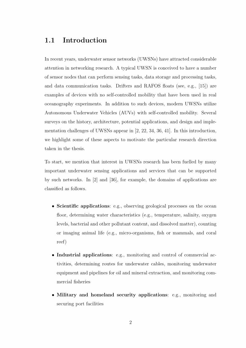
1.1 Introduction

In recent years, underwater sensor networks (UWSNs) have attracted considerable

attention in networking research. A typical UWSN is conceived to have a number

of sensor nodes that can perform sensing tasks, data storage and processing tasks,

and data communication tasks. Drifters and RAFOS floats (see, e.g., [15]) are

examples of devices with no self-controlled mobility that have been used in real

oceanography experiments. In addition to such devices, modern UWSNs utilize

Autonomous Underwater Vehicles (AUVs) with self-controlled mobility. Several

surveys on the history, architecture, potential applications, and design and imple-

mentation challenges of UWSNs appear in [2, 22, 34, 36, 41]. In this introduction,

we highlight some of these aspects to motivate the particular research direction

taken in the thesis.

To start, we mention that interest in UWSNs research has been fuelled by many

important underwater sensing applications and services that can be supported

by such networks. In [2] and [36], for example, the domains of applications are

classified as follows.

• Scientific applications: e.g., observing geological processes on the ocean

floor, determining water characteristics (e.g., temperature, salinity, oxygen

levels, bacterial and other pollutant content, and dissolved matter), counting

or imaging animal life (e.g., micro-organisms, fish or mammals, and coral

reef)

• Industrial applications: e.g., monitoring and control of commercial ac-

tivities, determining routes for underwater cables, monitoring underwater

equipment and pipelines for oil and mineral extraction, and monitoring com-

mercial fisheries

• Military and homeland security applications: e.g., monitoring and

securing port facilities

2

• Humanitarian applications: e.g., search and survey missions, disaster

prevention tasks (e.g., tsunami warning to coastal area), identification of

seabed hazards, locating dangerous rocks or shoals, and identifying possible

mooring locations

UWSNs are expected to provide better services in each of the above domains

over the traditional approach of deploying underwater sensor devices that record

data during a monitoring mission, and then recovering the devices at the end of a

mission. In [2], the authors point out that compared to this traditional approach,

UWSNs provide the following advantages:

• supporting real time monitoring, since the observed data can be transmitted

shortly after collection,

• supporting better interaction between onshore control systems and the mon-

itoring devices, and

• supporting better handling of device failures and misconfigurations.

It has also been emphasized in the above survey papers that UWSNs are expected

to be sparser than terrestrial wireless sensor networks (WSNs) since individual

nodes in UWSNs have significantly more cost compared to nodes in terrestrial

WSNs. In addition, many UWSNs are required to cover relatively larger water

areas.

The design and implementation of cost effective UWSNs to serve the above ap-

plications, however, face a number of challenges. Some of these challenges are

attributed to the current technological limitations of dealing with the underwater

communication channel. Other challenges are attributed to the harsh environment

of underwater environments.

Challenges of the underwater communication channel. Unlike terrestrial-

based WSNs that enjoy low delay and high bandwidth networking devices, UWSNs

face significant challenges in getting adequate communication bandwidth. To see

this, we summarize below some of the findings emphasized in [41] and [2] on

3

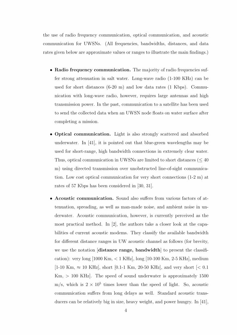
the use of radio frequency communication, optical communication, and acoustic

communication for UWSNs. (All frequencies, bandwidths, distances, and data

rates given below are approximate values or ranges to illustrate the main findings.)

• Radio frequency communication. The majority of radio frequencies suf-

fer strong attenuation in salt water. Long-wave radio (1-100 KHz) can be

used for short distances (6-20 m) and low data rates (1 Kbps). Commu-

nication with long-wave radio, however, requires large antennas and high

transmission power. In the past, communication to a satellite has been used

to send the collected data when an UWSN node floats on water surface after

completing a mission.

• Optical communication. Light is also strongly scattered and absorbed

underwater. In [41], it is pointed out that blue-green wavelengths may be

used for short-range, high bandwidth connections in extremely clear water.

Thus, optical communication in UWSNs are limited to short distances (≤ 40

m) using directed transmission over unobstructed line-of-sight communica-

tion. Low cost optical communication for very short connections (1-2 m) at

rates of 57 Kbps has been considered in [30, 31].

• Acoustic communication. Sound also suffers from various factors of at-

tenuation, spreading, as well as man-made noise, and ambient noise in un-

derwater. Acoustic communication, however, is currently perceived as the

most practical method. In [2], the authors take a closer look at the capa-

bilities of current acoustic modems. They classify the available bandwidth

for different distance ranges in UW acoustic channel as follows (for brevity,

we use the notation [distance range, bandwidth] to present the classifi-

cation): very long [1000 Km, < 1 KHz], long [10-100 Km, 2-5 KHz], medium

[1-10 Km, ≈ 10 KHz], short [0.1-1 Km, 20-50 KHz], and very short [< 0.1

Km, > 100 KHz]. The speed of sound underwater is approximately 1500

m/s, which is 2 × 105 times lower than the speed of light. So, acoustic

communication suffers from long delays as well. Standard acoustic trans-

ducers can be relatively big in size, heavy weight, and power hungry. In [41],

4

the authors point out that on compact stationary sensor nodes, and space-

constraint AUVs, transducers generally cannot be spatially separated far

enough to provide full-duplex connections since the transmitted signals will

saturate the receiver even when the communication bands are fairly widely

separated. Thus, underwater networks are expected to utilize half-duplex

connections.

The above challenges in supporting low delay and high data rate communication

have triggered research work in almost all areas of the UW networking protocol

stack. The following surveys are particular to UWSNs: Medium Access Control

(MAC) protocols [21, 29, 42, 55, 57], routing [8, 9, 33, 44], localization [20, 26, 52,

58, 59], connectivity and coverage [32, 60]. Examples of research work done on

connectivity, coverage, and deployments appear in [1, 3, 4, 48, 50].

Challenges due to node mobility. To serve the diverse types of applications

mentioned above, various types of UWSN deployments are used. In [36], for

example (see, e.g., figure 1.1), UWSN deployments are classified as being either

static, semi-mobile, or mobile. Static networks have nodes attached to underwater

ground, anchored buoys, or docks. Semi-mobile networks may have collection of

nodes attached to a free floating buoy. Nodes in semi-mobile networks are subject

to small scale movements. Mobile networks may be composed of drifters with no

self mobility capability, or nodes with mobility capability. Nodes in such networks

are subject to large scale movements. UWSN deployments may occur over many

short periods of times (e.g., several days at a time), so as to conduct several

missions over a large area of interest. Maintaining connectivity in such networks

is a crucial aspect for performing many tasks that require node collaboration.

Examples of such tasks include localization [26, 27, 37, 53, 58, 59], routing [39, 40,

47, 56] and coverage [1, 4, 43, 50].

In this thesis, we consider semi-mobile and mobile networks. Our interest is in

developing methodologies that allow a designer to analyze the likelihood that a

network (or part of it) is connected at a given time interval. In the next section,

5

 

Tether underwater node Free floating underwater node 

Figure 1.1: Example UWSNs.

we review some work on quantifying node mobility models used by networking

researchers for UWSNs.

1.2 Node Mobility

One may classify node mobility in UWSNs into controllable mobility (C-mobility

for short), and uncontrollable mobility (U-mobility). The simplest type of C-

mobility is vertical movements induced by mechanical devices inside a node [27,

28]. Full 3D C-mobility is enjoyed by AUVs at the expense of node energy con-

sumption. U-mobility, on the other hand, is primarily due to surface and sub-

surface water currents, as well as wind. Findings of real ocean measurements,

as well as a large body of analytical results in oceanography have shaped the

understanding of networking researchers in this area.

We note that this area is new to networking researchers where the obtained ana-

lytical results are rooted in the mathematically deep field of fluid dynamics. The

thesis work makes an effort to summarize some of the important findings in this

regard. Our goal in this section is to foster the idea that numerical values for the

probabilistic locality model used throughout the thesis can be deduced from the

available empirical measurements of node mobility, and the obtained analytical

models that capture the behaviour found in the empirical results.

6

The probabilistic node locality adopted in the thesis divides the geographic area

containing nodes into rectangles of an (imaginary) superimposed grid layout. After

a given time period following network deployment in water, each node x can be in

any one of a possible set of grid rectangles, denoted Loc(x) = {x[1], x[2], . . .}. We

call Loc(x) the locality set of x. Thus, depending on the mobility model induced

by water currents, node x can be in any possible grid rectangle x[i] ∈ Loc(x) with

a certain probability, denoted px(i).

To explain that such probability distribution can be deduced from empirical ex-

periments, we refer to the important work of [15] which has triggered intensive

work in the area. In [15], the authors report on several observations collected in

the Gulf Stream using thirty-seven RAFOS drifters launched off Cape Hatteras.

Mobility of the free floating drifters is tracked for 30 or 45 days. Among the

collected observations, the authors determined the geographic location of each of

the 37 drifters at each day of the observation period. Given the exact geographic

location of each drifter in each day, one can superimpose a virtual grid (of some

user specified dimensions per rectangle) on the area traversed by the floats and

use the reported locations to derive rough values of the probabilities used in our

probabilistic locality model.

Next, we present our findings on the use of the available analytical mobility models

to derive the probabilities used in our model. In [15], the authors observed striking

patterns of cross-stream and vertical motion associated with meanders in the Gulf

Stream. Later, in [14], the author introduced a 2D kinematic model that captures

many of the important patterns observed in [15] including the effect of meandering

sub-surface currents and vortices on free floating drifters. The introduction of

such kinematic model has resulted in a large body of subsequent analytical work

in the area. Recently, this kinematic model has received attention in networking

literature. Following a similar approach, [18] devised a kinematic mobility model

for UWSNs, called the meandering current mobility model. The model is useful

for large coastal environments that span several kilometres. It captures the strong

correlations in mobility of nearby sensor nodes. In [18], the model has been used to

7

analyze several network connectivity, coverage, and localization aspects of UWSNs

by simulation.

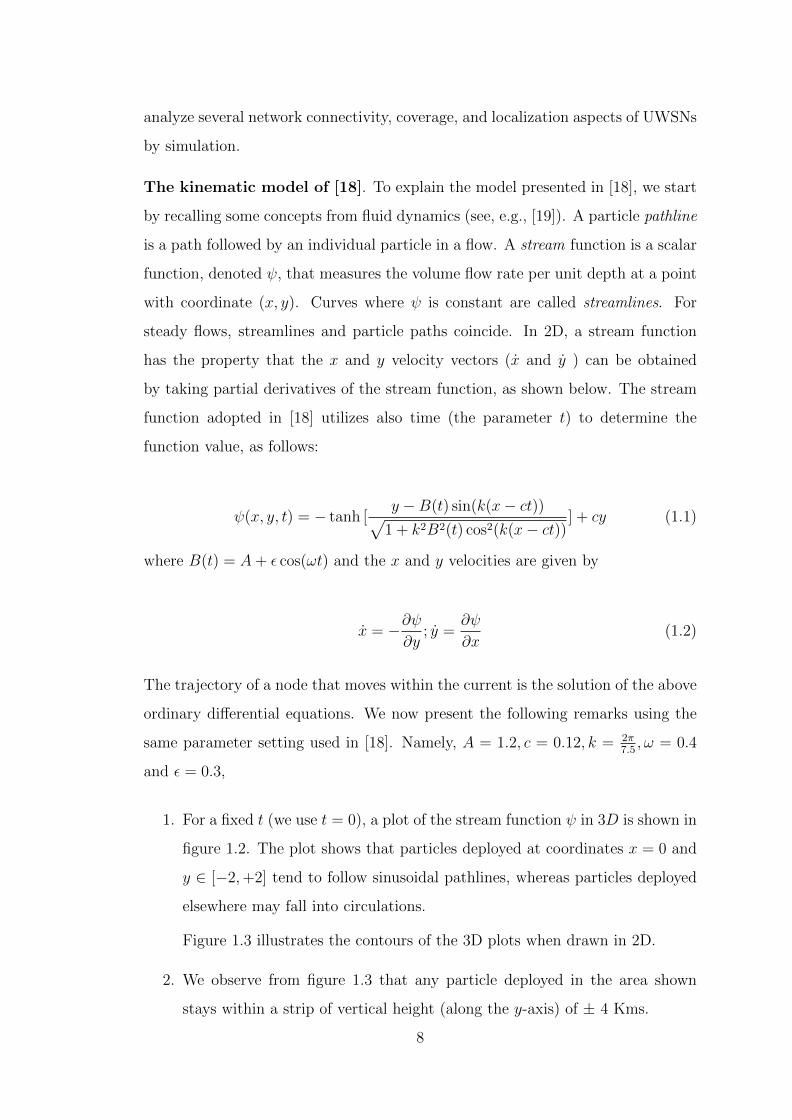
The kinematic model of [18]. To explain the model presented in [18], we start

by recalling some concepts from fluid dynamics (see, e.g., [19]). A particle pathline

is a path followed by an individual particle in a flow. A stream function is a scalar

function, denoted ψ, that measures the volume flow rate per unit depth at a point

with coordinate (x, y). Curves where ψ is constant are called streamlines. For

steady flows, streamlines and particle paths coincide. In 2D, a stream function

has the property that the x and y velocity vectors (x and y ) can be obtained

by taking partial derivatives of the stream function, as shown below. The stream

function adopted in [18] utilizes also time (the parameter t) to determine the

function value, as follows:

ψ(x, y, t) = − tanh [y −B(t) sin(k(x− ct))√

1 + k2B2(t) cos2(k(x− ct))] + cy (1.1)

where B(t) = A+ ε cos(ωt) and the x and y velocities are given by

x = −∂ψ∂y

; y =∂ψ

∂x(1.2)

The trajectory of a node that moves within the current is the solution of the above

ordinary differential equations. We now present the following remarks using the

same parameter setting used in [18]. Namely, A = 1.2, c = 0.12, k = 2π7.5, ω = 0.4

and ε = 0.3,

1. For a fixed t (we use t = 0), a plot of the stream function ψ in 3D is shown in

figure 1.2. The plot shows that particles deployed at coordinates x = 0 and

y ∈ [−2,+2] tend to follow sinusoidal pathlines, whereas particles deployed

elsewhere may fall into circulations.

Figure 1.3 illustrates the contours of the 3D plots when drawn in 2D.

2. We observe from figure 1.3 that any particle deployed in the area shown

stays within a strip of vertical height (along the y-axis) of ± 4 Kms.

8

ψ

Figure 1.2: A 3D plot of stream function 1.1

Figure 1.3: A plot of stream function 1.1 at t = 0.

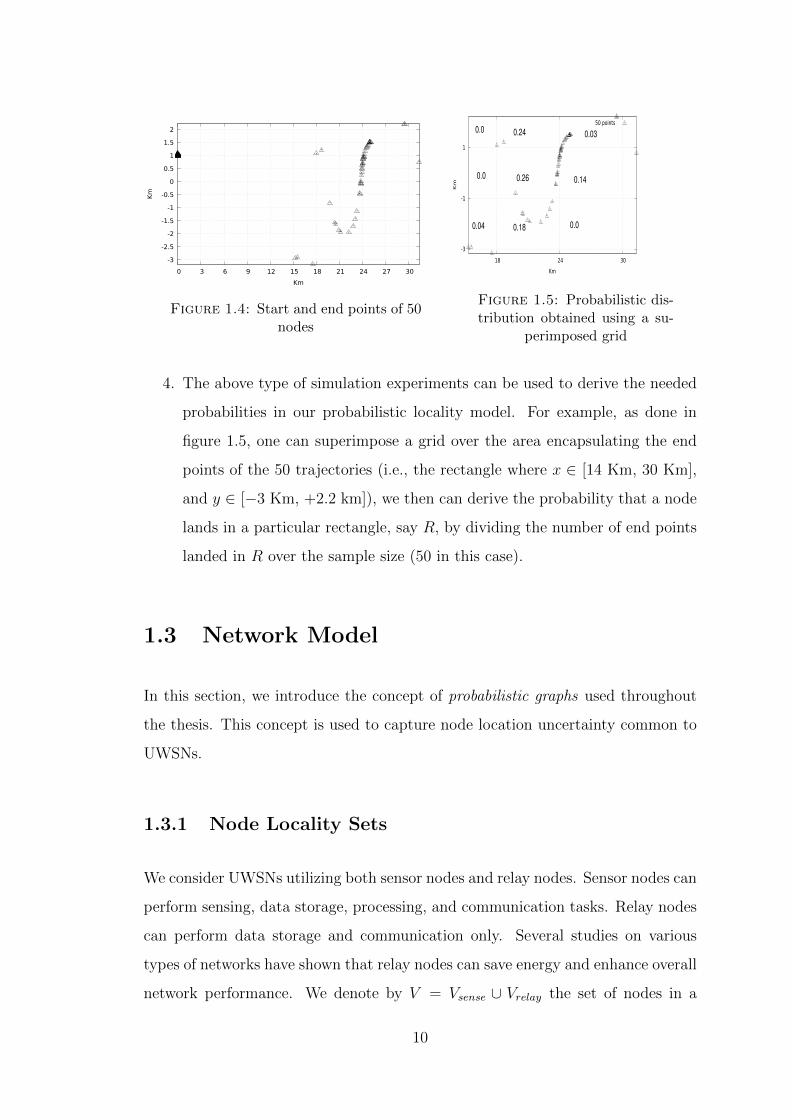
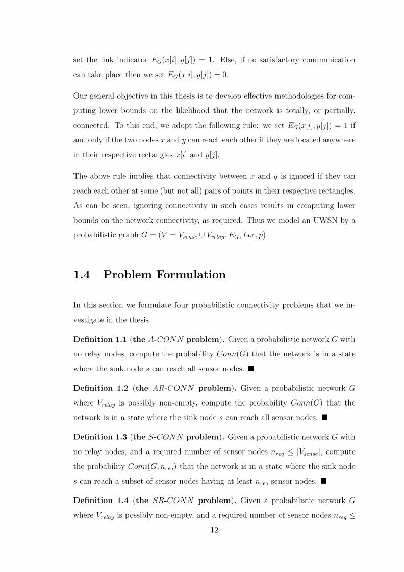
3. Although the above ordinary differential equations are deterministic, small

variations in the initial position of a node deployed at t=0 has a strong

influence on the trajectory taken by the node (e.g., which circulations it falls

into, and for how long). Figure 1.4 illustrates the findings of an experiment

where a sample set of 50 nodes are deployed at t = 0 in a rectangle of narrow

horizontal width at x = 0, and vertical height in the range y ∈ [1.00, 1.30]

(300 meters). The trajectories are simulated for 2 days. The figure shows

the initial positions of the 50 nodes on the left, and the end points of the

trajectories at the end of the 2-day period.

9

-3

-2.5

-2

-1.5

-1

-0.5

0

0.5

1

1.5

2

0 3 6 9 12 15 18 21 24 27 30

Km

Km

Figure 1.4: Start and end points of 50nodes

-3

-1

1

18 24 30

Km

Km

50 points

0.04 0.18 0.0

0.0 0.26 0.14

0.030.240.0

Figure 1.5: Probabilistic dis-tribution obtained using a su-

perimposed grid

4. The above type of simulation experiments can be used to derive the needed

probabilities in our probabilistic locality model. For example, as done in

figure 1.5, one can superimpose a grid over the area encapsulating the end

points of the 50 trajectories (i.e., the rectangle where x ∈ [14 Km, 30 Km],

and y ∈ [−3 Km, +2.2 km]), we then can derive the probability that a node

lands in a particular rectangle, say R, by dividing the number of end points

landed in R over the sample size (50 in this case).

1.3 Network Model

In this section, we introduce the concept of probabilistic graphs used throughout

the thesis. This concept is used to capture node location uncertainty common to

UWSNs.

1.3.1 Node Locality Sets

We consider UWSNs utilizing both sensor nodes and relay nodes. Sensor nodes can

perform sensing, data storage, processing, and communication tasks. Relay nodes

can perform data storage and communication only. Several studies on various

types of networks have shown that relay nodes can save energy and enhance overall

network performance. We denote by V = Vsense ∪ Vrelay the set of nodes in a

10

given UWSN where Vsense denotes sensor nodes, and Vrelay denotes relay nodes.

We assume that Vsense has a distinguished sink node, denoted s, that performs

network wide command and control functions.

After some time interval T from network deployment time, each node x can be in

some location determined by water currents causing node movement.

To simplify analysis, current approaches in the literature typically divide the geo-

graphic area containing nodes into rectangles of a superimposed grid layout. Thus,

at time T, each node x can be in any one of a possible set of grid rectangles denoted

Loc(x) = {x[1], x[2], . . .}. We call Loc(x) the locality set of x (for simplicity, we

omit the dependency on T from the notation). Depending on the mobility model

induced by water currents, node x can be in any possible grid rectangle x[i] with

a certain probability, denoted px(i).

As mentioned in Section 1.2, one may utilize the kinematic model adopted in [18]

to compute such probabilities from a sufficiently large number of node trajectories

simulated by the model.

Henceforth, we use x[i] to refer to node x at the ith location index. For brevity, we

also refer to x[i] as the location of x (rather than the grid rectangle containing x)

at an instant of interest. To gain efficiency in solving large problem instances with

large locality sets, it may be convenient to truncate some locality sets to include

only locations of high occurrence probability, and ignore the remaining locations.

In such cases, we get∑

x[i]∈Loc(x) px(i) ≤ 1, if Loc(x) is truncated.

1.3.2 Node Reachability

At any instant, node x can reach node y if the acoustic signal strength from x to y

(and vice versa) exceeds a certain threshold value. In acoustic UWSN, direction of

water currents play an important role in signal delay (see, e.g., [46]). For simplicity,

we assume that given the exact locations of x and y, say x at location x[i] and y

at location y[j], we can determine if x and y can reach each other, and if so, we

11

set the link indicator EG(x[i], y[j]) = 1. Else, if no satisfactory communication

can take place then we set EG(x[i], y[j]) = 0.

Our general objective in this thesis is to develop effective methodologies for com-

puting lower bounds on the likelihood that the network is totally, or partially,

connected. To this end, we adopt the following rule: we set EG(x[i], y[j]) = 1 if

and only if the two nodes x and y can reach each other if they are located anywhere

in their respective rectangles x[i] and y[j].

The above rule implies that connectivity between x and y is ignored if they can

reach each other at some (but not all) pairs of points in their respective rectangles.

As can be seen, ignoring connectivity in such cases results in computing lower

bounds on the network connectivity, as required. Thus we model an UWSN by a

probabilistic graph G = (V = Vsense ∪ Vrelay, EG, Loc, p).

1.4 Problem Formulation

In this section we formulate four probabilistic connectivity problems that we in-

vestigate in the thesis.

Definition 1.1 (the A-CONN problem). Given a probabilistic network G with

no relay nodes, compute the probability Conn(G) that the network is in a state

where the sink node s can reach all sensor nodes. �

Definition 1.2 (the AR-CONN problem). Given a probabilistic network G

where Vrelay is possibly non-empty, compute the probability Conn(G) that the

network is in a state where the sink node s can reach all sensor nodes. �

Definition 1.3 (the S-CONN problem). Given a probabilistic network G with

no relay nodes, and a required number of sensor nodes nreq ≤ |Vsense|, compute

the probability Conn(G, nreq) that the network is in a state where the sink node

s can reach a subset of sensor nodes having at least nreq sensor nodes. �

Definition 1.4 (the SR-CONN problem). Given a probabilistic network G

where Vrelay is possibly non-empty, and a required number of sensor nodes nreq ≤12

|Vsense|, compute the probability Conn(G, nreq) that the network is in a state where

the sink node s can reach a subset of sensor nodes having at least nreq sensor nodes.

�

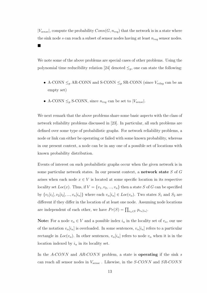
We note some of the above problems are special cases of other problems. Using the

polynomial time reducibility relation [24] denoted ≤p, one can state the following:

• A-CONN ≤p AR-CONN and S-CONN ≤p SR-CONN (since Vrelay can be an

empty set)

• A-CONN ≤p S-CONN, since nreq can be set to |Vsense|.

We next remark that the above problems share some basic aspects with the class of

network reliability problems discussed in [23]. In particular, all such problems are

defined over some type of probabilistic graphs. For network reliability problems, a

node or link can either be operating or failed with some known probability, whereas

in our present context, a node can be in any one of a possible set of locations with

known probability distribution.

Events of interest on such probabilistic graphs occur when the given network is in

some particular network states. In our present context, a network state S of G

arises when each node x ∈ V is located at some specific location in its respective

locality set Loc(x). Thus, if V = {v1, v2, ..., vn} then a state S of G can be specified

by {v1[i1], v2[i2], ..., vn[in]} where each vα[iα] ∈ Loc(vα). Two states S1 and S2 are

different if they differ in the location of at least one node. Assuming node locations

are independent of each other, we have Pr(S) =∏

vα∈V pvα[iα].

Note: For a node vα ∈ V and a possible index iα in the locality set of vα, our use

of the notation vα[iα] is overloaded. In some sentences, vα[iα] refers to a particular

rectangle in Loc(vα). In other sentences, vα[iα] refers to node vα when it is in the

location indexed by iα in its locality set.

In the A-CONN and AR-CONN problem, a state is operating if the sink s

can reach all sensor nodes in Vsense . Likewise, in the S-CONN and SR-CONN

13

problem, a state S is operating if the sink node s can reach a subset having

at least nreq sensor nodes. Let S be the set of all operating states S of a given

problem. Then the required solution is given by∑

S∈S Pr(S).

Example 1.1. Figure 1.6 illustrates a probabilistic graph on 4 nodes where V =

{s, a, b, c} and the locality set of each node has 2 locations. The network has 24

states. For the A-CONN problem, state S1 = {s[2], a[2], b[2], c[2]} is operating,

and state S2 = {s[1], a[1], b[1], c[2]} is failed. �

s[1] s[2]

0.5 0.5b[1] b[2]

0.5 0.5

0.50.5

a[1]

a[2]

0.50.5

c[1]

c[2]s[1] s[2]

0.5 0.5b[1] b[2]

0.50.5

a[1]

a[2]

0.50.5

c[1]

c[2]sink

Figure 1.6: An example probabilistic network

The Underlying Graph of Probabilistic Network. Given a probabilistic

network G = (V,EG, Loc, p) the underlying graph of G is an undirected graph G

where

1. V (G) = V .

2. E(G) has an edge e = (x, y) if for some positions x[i] and y[j] of nodes x

and y, respectively, we have EG(x[i], y[j]) = 1.

Example 1.2. The underlying graph of the probabilistic network in figure 1.6 is

the cycle (s, a, c, b). �

Equivalently, we say that the probabilistic network G has the topology of the

graph G. Throughout the thesis, we use the same symbol G to refer to both a

probabilistic network and its underlying graph. Overloading the use of the symbol

G does not cause confusion since the exact meaning can be deduced by context.

14

1.5 Thesis Organization and Contribution

The main research direction undertaken in the thesis is to develop efficient algo-

rithms for handling the defined probabilistic connectivity problems on networks

whose underlying graphs have some useful structure. The availability of such al-

gorithms can be used to derive lower bounds on the probabilistic connectivity

of any given arbitrary probabilistic network. This approach relies on identifying

subgraphs with the desired structure in the graph underlying a given probabilis-

tic network then solving a problem of interest on the identified subgraph. The

thesis pursues this general approach on the well known classes of partial k-trees,

explained in Chapter 2. The remaining part of the thesis is organized as follows.

1. Chapter 2 is dedicated to reviewing basic definitions, properties, and algo-

rithmic aspects of k-trees and partial k-trees.

2. Chapter 3 presents the first contribution of the thesis: an efficient dynamic

programming algorithm to solve the SR-CONN problem on probabilistic

networks whose underlying graphs are trees. The algorithm solves the more

restricted AR-CONN problem with little overhead compared to a dedicated

algorithm to solve the AR-CONN problem.

3. Chapter 4 presents a second contribution of the thesis: a dynamic program-

ming algorithm to solve the A-CONN problem on partial k-trees. The algo-

rithm runs in polynomial time for any fixed k.

4. Chapter 5 considers UWSNs with relay nodes. The chapter presents a third

contribution: two dynamic programming algorithms to solve the AR-CONN

and SR-CONN problems on partial k-trees. The algorithm runs in polyno-

mial time for any fixed k.

Finally Chapter 6 concludes with remarks and possible future research directions

15

1.6 Concluding Remarks

In this chapter, we have introduced the notion of a probabilistic network that

captures node location uncertainty commonly encountered in UWSNs. Using the

notion of probabilistic networks, we have formalized 4 concrete probabilistic con-

nectivity problems whose solution can significantly benefit the design of UWSNs

utilizing relay nodes. In the next chapter, we introduce the class of partial k-tree

that enable the computation of lower bounds on the probabilistic connectivity

problems of interest.

16

Chapter 2

Algorithmic Aspects of k-Trees

In this chapter, we review basic definitions and properties of a hi-

erarchy of graph classes known as k-trees, where k ≥ 1. Several impor-

tant classes of graphs are known to be special cases of partial k-trees,

for k = 1, 2, 3, and 4. Also, several NP-complete problems have been

shown to admit polynomial time algorithms on partial k-trees, when

k is fixed. Our main contributions in the next chapters show that

the probabilistic connectivity problems introduced in Chapter 1 also

admit similar polynomial time algorithms. As an introduction to the

algorithmic ideas used in subsequent chapters, we review an algorithm

due to [54] for solving the Steiner tree problem on partial 2-trees. We

conclude by discussing known results on extracting a partial k-tree

subgraph, with prescribed k, from an arbitrary given network.

2.1 Graph Notation

In this section, we introduce a few graph theoretic notations that we need through-

out the thesis. In general, we adopt the same notation used, for example, in [24]

and other books. An undirected graph G = (V,E) has a set V of nodes (or ver-

tices), and a set E of edges (or links). We also use V (G) and VG to denote the set

17

of nodes. Likewise, we use E(G) and EG to denote the set of edges.

We also need the following notation.

• degG(v): the degree of node v in graph G

• NG(v): the set of neighbouring nodes of v in G

• An induced subgraph G′ ⊆ G on a set V ′ ⊆ V of nodes contains all edges of

G where the two end nodes of each edge lie in V ′.

• A clique is a complete graph, and a k-clique is a clique on k nodes.

• A separator in G is a subset of nodes whose removal disconnects G into two,

or more, connected components.

2.2 k-Trees and Partial k-Trees

k-Trees. The formulation of k-trees dates back to the work of [10, 11] as a

generalization of conventional trees. A recursive definition is given below.

Definition 2.1. For a given integer k ≥ 1, the class of k-trees is defined as follows

1. A k-clique is a k-tree.

2. If Gn is a k-tree on n nodes then so is the graph Gn+1 obtained by adding a

new node, and making it adjacent to every node in k-clique of Gn. �

Thus, trees are 1-trees. A k-leaf of a k-tree G on k + 1, or more, nodes is a node

whose neighbours induce a k-clique. By repeatedly deleting k-leaves form a k-tree

Gn, on n ≥ k nodes, one can reduce Gn to a k-clique. We call such a sequence of

nodes a k-leaf elimination sequence.

Example 2.1. Figure 2.1 illustrates a fragment of 3-tree G on n = 6 nodes. G

has a 3-leave vb. �

The following are basic properties of k-trees (for other properties, see e.g., [35] and

[45])

18

 

vi

vl

vk

vj

va

vb

Figure 2.1: A fragment of a 3-tree

Lemma 2.2.

1. Every k-tree that is not a complete graph has at least two non-adjacent

k-leaves.

2. Given a k-tree G and a k-clique subgraph H of G, there exists a k-leaf

elimination sequence that reduces G to H.

3. Given two non-adjacent nodes u and v of a k-tree G, a subgraph induced on

any minimal (u, v)-separator is a k-clique. �

Partial k-Trees. A partial k-tree is a k-tree possibly missing some edges. The

classes of partial k-trees, for k = 1, 2, 3, . . ., form a hierarchy of graphs since any

partial k-tree is also a partial k + 1-tree. A leaf of a partial k-tree G is a node

x that is a k-leaf in some embedding of G in a k-tree G (thus, degG(x) ≤ k). A

perfect elimination of a node x from G is the elimination of x and its incident

edges and the addition of the necessary edges to complete NG(x) to a clique. A

k-perfect elimination sequence (k-PES) of a graph G is an ordering (v1, v2, . . . , vr)

of V (G) such that

1. degG(v1) ≤ k, and

2. for i = 2, 3, . . . , the degree of vi is obtained by removing the sequence

v1, . . . , vi−1 is at most k.

Example 2.2. For the graph G in figure 2.2, (va, vb, vi, vj, vk, vl) is a 3-PES. �

Every partial k-tree G has a k-PES. Similar to Lemma 2.2 (1), every partial k-

tree that is not a complete graph has at least two non-adjacent leaves. In Chapters

19

 

vi

vl

vk

vj

va

vb

Figure 2.2: A partial 3-tree

4 and 5, G is a partial k-tree, for some k, of some sensor network that contains a

sink node s. In any completion of G to a k-tree G, the sink node appears in some

k-clique H. By lemma 2.2, one can find a k-PES such that the sink node is the

last node in the sequence. We henceforth deal with such k-PES.

Graphs with Bounded Tree-width. The work in [49] has introduced the

concept of graphs with bounded tree-width in the context of resolving a particular

graph theoretic conjecture. The concept is defined as follows.

Definition 2.3. [49] A tree-decomposition of a graph G is a family (Xi : i ∈ I)

of subsets of V (G), together with a tree T with V (T ) = I, with the following

properties.

1.⋃

i∈IXi = V (G).

2. Every edge of G has both its ends in some Xi.

3. For i, j, k ∈ I, if j lies on the path of T from i to k then Xi ∩Xk ⊆ Xj. �

Definition 2.4. The width of a tree-decomposition is max(|Xi| − 1 : i ∈ I). �

Definition 2.5. The tree-width of G is the minimum w ≥ 0 such that G has a

tree-decomposition of width ≤ w. �

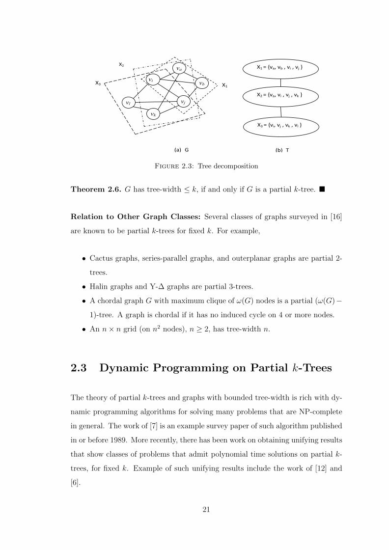
Example 2.3. Figure 2.3(a) illustrates a graph G having a tree-decomposition

shown in figure 2.3(b). The width of the tree decomposition is 3. One may verify

that 3 is actually the tree-width of G. �

The following result is mentioned in [16].

20

 

X3 vi

vl

vk

vj

va

vb

X2 

X1 

(a) G

X1 = {va, vb , vi , vj } 

X2 = {va, vi , vj , vk } 

X3 = {vi, vj , vk , vl } 

(b) T 

Figure 2.3: Tree decomposition

Theorem 2.6. G has tree-width ≤ k, if and only if G is a partial k-tree. �

Relation to Other Graph Classes: Several classes of graphs surveyed in [16]

are known to be partial k-trees for fixed k. For example,

• Cactus graphs, series-parallel graphs, and outerplanar graphs are partial 2-

trees.

• Halin graphs and Y-∆ graphs are partial 3-trees.

• A chordal graph G with maximum clique of ω(G) nodes is a partial (ω(G)−1)-tree. A graph is chordal if it has no induced cycle on 4 or more nodes.

• An n× n grid (on n2 nodes), n ≥ 2, has tree-width n.

2.3 Dynamic Programming on Partial k-Trees

The theory of partial k-trees and graphs with bounded tree-width is rich with dy-

namic programming algorithms for solving many problems that are NP-complete

in general. The work of [7] is an example survey paper of such algorithm published

in or before 1989. More recently, there has been work on obtaining unifying results

that show classes of problems that admit polynomial time solutions on partial k-

trees, for fixed k. Example of such unifying results include the work of [12] and

[6].

21

The approach used in such results relies on formalizing graph and network prop-

erties as logical statements in a particular logic system. Such approaches are not

intended to provide optimized algorithms for solving any particular problem at

hand, or implementing a direct solution. It is often more fruitful to construct a di-

rect algorithm for handling a given problem of interest. In the rest of the section,

we review a dynamic programming algorithm result due to [54] for solving the

Steiner tree problem on partial 2-trees. This dynamic programming algorithm has

inspired the design of many subsequent algorithms for solving other NP-complete

problems on partial k-trees. A Steiner tree can be defined as follows.

Definition 2.7. Given a graph G = (V,E) with positive integer edge costs, and a

set of target nodes Vtarget ⊆ V , a Steiner tree, denoted ST (G, Vtarget), is a subtree

G′ = (V ′, E ′) satisfying

1. Vtarget ⊆ V ′ ⊆ V ,

2. the sum of edge costs in E ′ is minimum over all subtrees satisfying (1). �

The algorithm devised in [54] works as follows. The graph is reduced by repeated

deletion of degree-2 vertices until the graph which remains is a single edge. During

this vertex elimination procedure, the algorithm summarize information about the

triangle {x, y, z} , where y has degree 2, on the arcs (x, z) and (z, x) , prior to

deleting y. This summary information encodes information about Steiner trees in

the subgraph of the 2-tree which has thus far been reduced onto the edge {x, z}.With each edge α = (x, y) of G, the algorithm associates six cost measures, which

summarize the cost incurred so far of the subgraph S which has been reduced onto

the edge (x, y) [54]:

1. st(α) is the minimum cost of a Steiner tree for S, in which x and y appear

in the same tree.

2. dt(α) is the minimum cost of two disjoint trees for S including all targets,

one tree involving x and the other y.

3. yn(α) is the minimum cost of a Steiner tree for S, which includes x but not

y.

22

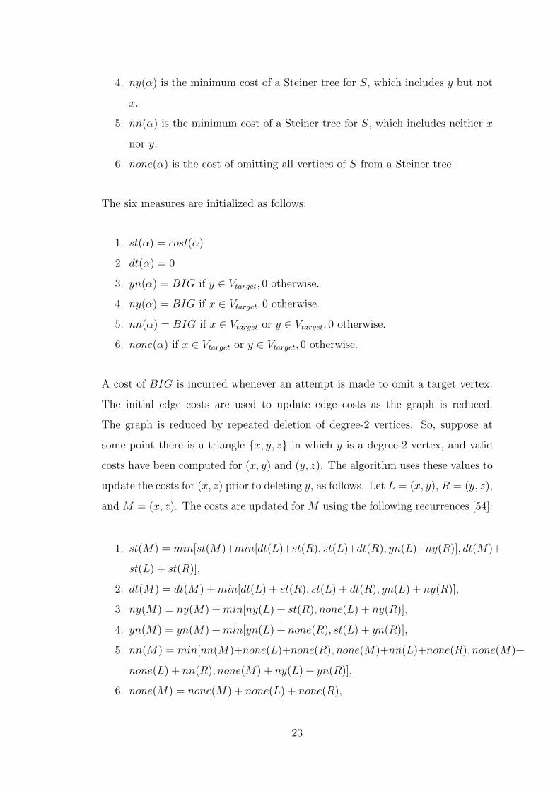
4. ny(α) is the minimum cost of a Steiner tree for S, which includes y but not

x.

5. nn(α) is the minimum cost of a Steiner tree for S, which includes neither x

nor y.

6. none(α) is the cost of omitting all vertices of S from a Steiner tree.

The six measures are initialized as follows:

1. st(α) = cost(α)

2. dt(α) = 0

3. yn(α) = BIG if y ∈ Vtarget, 0 otherwise.

4. ny(α) = BIG if x ∈ Vtarget, 0 otherwise.

5. nn(α) = BIG if x ∈ Vtarget or y ∈ Vtarget, 0 otherwise.

6. none(α) if x ∈ Vtarget or y ∈ Vtarget, 0 otherwise.

A cost of BIG is incurred whenever an attempt is made to omit a target vertex.

The initial edge costs are used to update edge costs as the graph is reduced.

The graph is reduced by repeated deletion of degree-2 vertices. So, suppose at

some point there is a triangle {x, y, z} in which y is a degree-2 vertex, and valid

costs have been computed for (x, y) and (y, z). The algorithm uses these values to

update the costs for (x, z) prior to deleting y, as follows. Let L = (x, y), R = (y, z),

and M = (x, z). The costs are updated for M using the following recurrences [54]:

1. st(M) = min[st(M)+min[dt(L)+st(R), st(L)+dt(R), yn(L)+ny(R)], dt(M)+

st(L) + st(R)],

2. dt(M) = dt(M) +min[dt(L) + st(R), st(L) + dt(R), yn(L) + ny(R)],

3. ny(M) = ny(M) +min[ny(L) + st(R), none(L) + ny(R)],

4. yn(M) = yn(M) +min[yn(L) + none(R), st(L) + yn(R)],

5. nn(M) = min[nn(M)+none(L)+none(R), none(M)+nn(L)+none(R), none(M)+

none(L) + nn(R), none(M) + ny(L) + yn(R)],

6. none(M) = none(M) + none(L) + none(R),

23

An alternative approach to present the above algorithm is to store the six measures

associated with edge α = (x, y) in a table, denoted Tx,y. The table provides

key-value mappings. Roughly speaking, the keys replace the use of some of the

names st, dt, yn, etc. with set notation. Not all names correspond to keys in this

formulation. Examples of names that correspond to keys are:

st = {x, y}1, dt = {x}1{y}1, yn = {x}1{y}0, and ny = {x}0{y}1.

As can be seen, each key contains a partition of the set {x, y}. To explain the

keys, let S be a subgraph reduced onto the edge α = (x, y) in some iteration of the

algorithm, and let S ′ ⊆ S be a subgraph of S that is a candidate for appearing in

a final solution. We now have:

• The key {x, y}1 is associated with a minimum cost S ′ such that both x and

y appear in one connected component of S ′, and this component has at least

one target node (counting x and y as possible target nodes).

• The key {x}1{y}0 is associated with a minimum cost S ′ such that x and

y appear in two different components of S ′, and only the component that

includes x contains one, or more, target nodes.

In this alternative approach, the above recurrences are replaced by functions that

merge 3 tables Tx,y, Ty,z and Tx,z into an updated Tx,z table.

2.4 Set Partitions

The dynamic programs devised in the rest of the thesis make heavy use of set parti-

tioning, as explained below. Given a setX, a partition ofX is a set {X1, X2, . . . , Xr},1 ≤ r ≤ |X| such that

1. X =⋃

i=1,2,...,r

Xi.

2. The Xis are pairwise disjoint.

24

In our algorithm, X is a set of nodes in a k-clique, and the partition of X are

used as part of states of dynamic programs. The number of all possible partition

of a set X on n elements are known as Bell numbers, denoted Bn (see for example

[17]). The first few Bell numbers are

B0 = B1 = 1, B2 = 2,

B3 = 5, B4 = 15, B5 = 52,

B6 = 203, B7 = 877, B8 = 4140, . . .

Bell numbers satisfy the following recurrence equation:

B0 = 1, B1 = 1 and Bn+1 =n∑

k=0

(n

k)Bk.

2.5 Finding Good Partial k-Tree Subgraphs

The algorithms presented in Chapters 3 to 5 can be used to derive lower bounds

on the Conn(G) and Conn(G, nreq) measures. This is done by

1. constructing a graph G that underlies the structure of a given probabilistic

graph of the problem instance at hand (as explained in subsequent chapters),

and

2. identifying a subgraph G′ of G that is a partial k-tree, of some user specified

k.

Under simple assumptions, we have Conn(G′) ≤ Conn(G) (or, Conn(G′, nreq) ≤Conn(G, nreq)). So Conn(G′), or Conn(G′, nreq), is a lower bound on the required

solution.

Ideally, one would prefer to use a subgrpah G′ that gives the best possible lower

bound. The problem of finding such subgraph is a complex graph problem. This

class of problems is related to the following classes of problems.

25

1. Recognizing Partial k-Trees: Given a graph G, and an integer k ≥ 1, is

G a partial k-tree?

• The work of [5] shows O(nk+2) algorithm for solving the problem. If k

is not fixed, then [5] shows that the problem is NP-complete.

• For any fixed k, the work of [13] improves on the above result by showing

a linear time recognition algorithm.

The above results produce also a k-PES if one exists.

2. Edge Deletion Problem (EDP) to Obtain a Partial k-Tree: Given a

graph G, and an integer k, find the minimum number of edges whose deletion

gives a partial k-tree.

• For k = 1, the problem is simple.

• For k ≥ 2, the problem is NP-complete (see, e.g. the work of [25] and

the references therein)

In the absence of known algorithms to find the required best subgraphs, we resort

to using heuristic algorithms. In Chapters 3 to 5, we experiment with partial

k-tree subgraphs (k = 1, 2, and 3) obtained using the following methods. We

assume that G is a connected graph.

The Random Method. Subgraphs obtained using the random method are

used as baseline cases for comparisons. This method constructs a partial k-tree

subgraph for k = 1, 2, and 3, as follows.

• Case k = 1. Choose any spanning tree.

• Case k = 2. Choose a spanning tree G′ ⊆ G. Fix an ordering of the

remaining edges not in G′. For each edge e in the fixed order, test whether

G′ + e is a partial 2-tree. If yes, add e to G′, and proceed to the next edge

in the fixed order.

26

• Case k = 3. Build a partial 2-tree G′ ⊆ G as in case k = 2, and let

S = (v1, v2, . . . , vn−2) be a 2-PES of G′. Fix an ordering of the edges not in

G′. For each edge e in the fixed order, test whether G′+ e is a partial 3-tree

with S being a 3-PES. If yes, add e to G′, and proceed to the next edge in

the fixed order.

The Greedy Method. Here, we associate with each link (x, y) ∈ EG a prob-

ability, denoted p(x, y), of having the link (x, y) present, given the locality sets

Loc(x) and Loc(y). For convenience of using a minimum spanning tree algorithm,

we transform each non-zero edge probability p(x, y) > 0 into edge cost using the

relation cost(x, y) = − log p(x, y). The greedy method constructs partial k-tree

subgraphs for k = 1, 2, and 3 as follows.

• Case k = 1: Choose a minimum spanning tree using the above edge costs.

• Case k = 2 and 3: As in cases k = 2 and 3, respectively, of the random

method, where we sort the remaining edges in a non-decreasing order of their

costs to obtain the fixed order

2.6 Concluding Remarks

In this chapter we have presented some background information on k-trees and

partial k-trees that serves as an introduction to the algorithms developed in sub-

sequent chapters.

27

Chapter 3

Probabilistic Connectivity of Tree

Networks

In this chapter, we consider the connectivity problems introduced in

Chapter 1 on probabilistic graphs that have the topology of a tree. We

present a dynamic programming algorithm to solve the SR-CONN

problem on such networks. The algorithm is designed to solve the more

restricted AR-CONN problem while incurring only a small overhead

compared to a specialized algorithm for solving the problem. Since

the SR-CONN problem is the most general problem among the four

problems defined in Chapter 1, it follows that the algorithm presented

in this chapter can solve the remaining three probabilistic connectivity

problems. Results in this chapter appear in our work in [38].

3.1 System Model

We recall that a probabilistic graph G = (V,EG, Loc, p) is specified by the follow-

ing:

• V = Vsense ∪ Vrelay the set of nodes in a given UWSN G

28

• EG(x[i], y[j]) = 1 if and only if the two nodes x and y can reach each other

when located anywhere in their respective rectangles x[i] and y[j]. This

restriction results in computing lower bounds on the solution since we ignore

cases where x and y can reach each other if they are located in some (but

not all) positions in their respective rectangles.

• Loc(v) is the locality set of node v.

• pv(i) is the probability that node v is located at grid rectangle v[i].

We say that the probabilistic graph G has the topology of a conventional tree

T = (V,ET ) if whenever EG(x[i], y[j]) = 1 then (x, y) ∈ ET . Note that the defini-

tion allows two nodes x and y to be adjacent in T , and yet they can take positions,

say x[i] and y[j], such that EG(x[i], y[j]) = 0. Thus, each state S of G gives a

subgraph of T .

In any such tree network T , one may safely delete a relay node x ∈ Vrelay that

appears as a leaf node without changing the problem solution. This observation

holds since relay nodes are relevant only if they connect some sensor node to the

sink s. We henceforth assume, without loss of generality, that the input network

G has no relay leaf.

We also recall that in the AR-CONN problem, a state is operating if the sink

s can reach all sensor nodes in Vsense. In the SR-CONN problem, a state S is

operating if the sink node s can reach a subset having at least nreq sensor nodes.

Let S be the set of all operating states S of a given AR-CONN or SR-CONN

problem then the required solution is given by∑

S∈S Pr(S).

3.2 Overview of the Algorithm

The algorithm (Function Conn in Figure 3.2) employs a dynamic programming

approach. It takes as input an instance (G, nreq) of the SR-CONN problem, and

29

a tree T = (V,ET ) on the set V of nodes with no relay leaves. The function

computes the exact solution Conn(G, nreq) of the given instance.

The pseudo-code uses syntax similar to C/C++ languages. In particular, we use

x ∗=y (or, x +=y) to mean x = x ∗ y (respectively, x = x+ y). We consider T as

a tree rooted at the sink s. Each node y in T except s has a parent node x on the

unique path from y to the root s. Each such node y is a root of a subtree, denoted

Ty = (Vy, ETy), obtained by removing the link (y, parent(y)) from T .

Example 3.1. Figure 3.1 illustrates a tree network where |Vsense| = 7 and |Vrelay| =3 nodes. Children(x2) = {y1, y2, y3} and subtree Ty3 has nodes {y3, z3, z4}�.

 

sensor node

relay node  s

x1 x2

y1

z2

z1

y2 y3

z4z3

Figure 3.1: A tree network

The key variables and data structures in the function are as follows.

• type(x): For any node x, type(x) = 0 if x is a relay node, and type(x) = 1 if

x is a sensor node.

• nsense(X): The number of sensor nodes in a given subset of nodes X ⊆ V .

We use nsense for nsense(V ).

• nrelay(X): The number of relay nodes in a given subset of nodes X ⊆ V . We

use nrelay for nrelay(V ).

• n(X) = nsense(X) + nrelay(X).

• nsense,min(X): The minimum number of sensor nodes in a given subset

X ⊆ V that should be connected to the sink in any operating state of

the overall network. So,

nsense,min(X) = max(0, nreq − nsense(X))

30

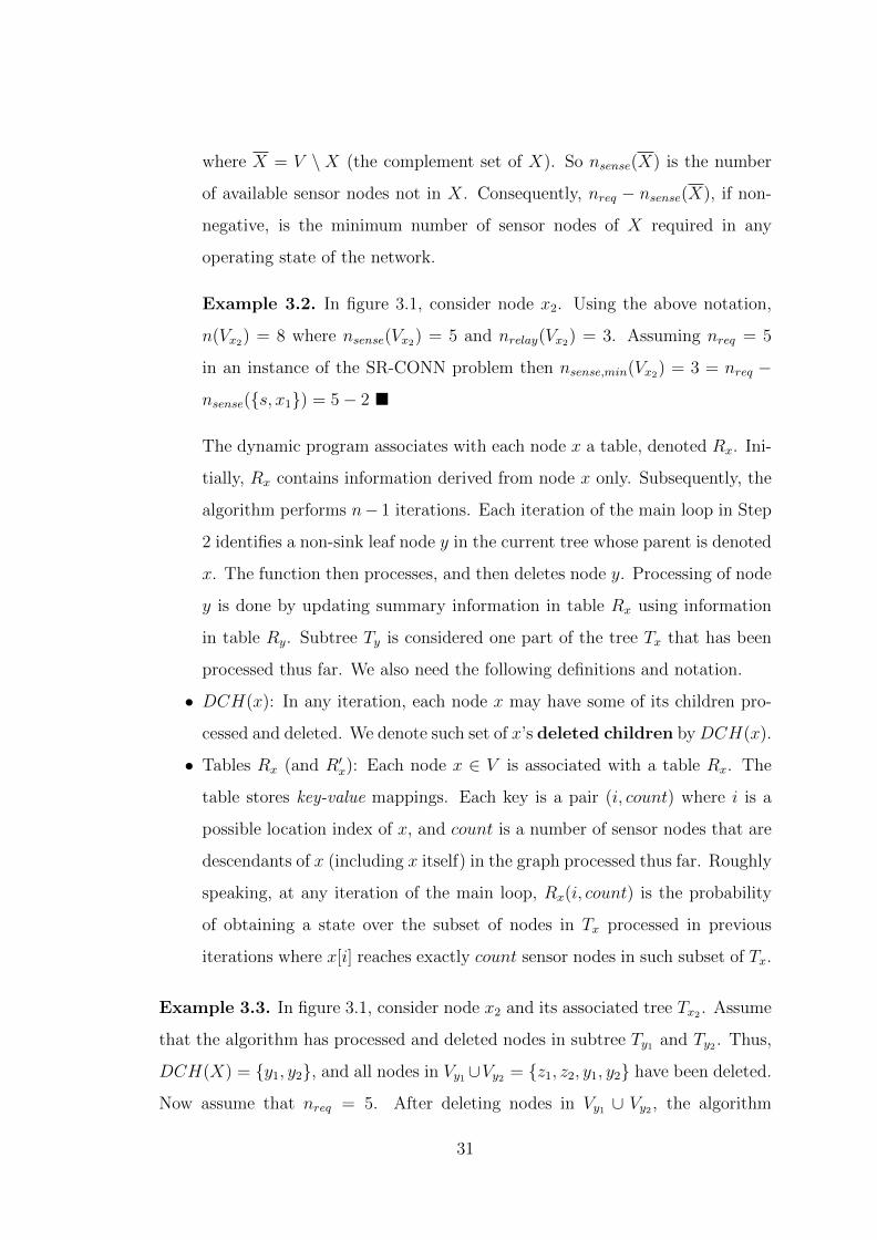
where X = V \ X (the complement set of X). So nsense(X) is the number

of available sensor nodes not in X. Consequently, nreq − nsense(X), if non-

negative, is the minimum number of sensor nodes of X required in any

operating state of the network.

Example 3.2. In figure 3.1, consider node x2. Using the above notation,

n(Vx2) = 8 where nsense(Vx2) = 5 and nrelay(Vx2) = 3. Assuming nreq = 5

in an instance of the SR-CONN problem then nsense,min(Vx2) = 3 = nreq −nsense({s, x1}) = 5− 2 �

The dynamic program associates with each node x a table, denoted Rx. Ini-

tially, Rx contains information derived from node x only. Subsequently, the

algorithm performs n− 1 iterations. Each iteration of the main loop in Step

2 identifies a non-sink leaf node y in the current tree whose parent is denoted

x. The function then processes, and then deletes node y. Processing of node

y is done by updating summary information in table Rx using information

in table Ry. Subtree Ty is considered one part of the tree Tx that has been

processed thus far. We also need the following definitions and notation.

• DCH(x): In any iteration, each node x may have some of its children pro-

cessed and deleted. We denote such set of x’s deleted children by DCH(x).

• Tables Rx (and R′x): Each node x ∈ V is associated with a table Rx. The

table stores key-value mappings. Each key is a pair (i, count) where i is a

possible location index of x, and count is a number of sensor nodes that are

descendants of x (including x itself) in the graph processed thus far. Roughly

speaking, at any iteration of the main loop, Rx(i, count) is the probability

of obtaining a state over the subset of nodes in Tx processed in previous

iterations where x[i] reaches exactly count sensor nodes in such subset of Tx.

Example 3.3. In figure 3.1, consider node x2 and its associated tree Tx2 . Assume

that the algorithm has processed and deleted nodes in subtree Ty1 and Ty2 . Thus,

DCH(X) = {y1, y2}, and all nodes in Vy1∪Vy2 = {z1, z2, y1, y2} have been deleted.

Now assume that nreq = 5. After deleting nodes in Vy1 ∪ Vy2 , the algorithm

31

computes

nsense,min({x2} ∪ Vy1 ∪ Vy2) = nreq − nsense({s, x1, y3, z3, z4})= 5− 4

= 1

This value is the minimum number of sensor nodes in the set X = {x2}∪Vy1 ∪Vy2required to be connected to the sink in any operating state of the overall graph.

�

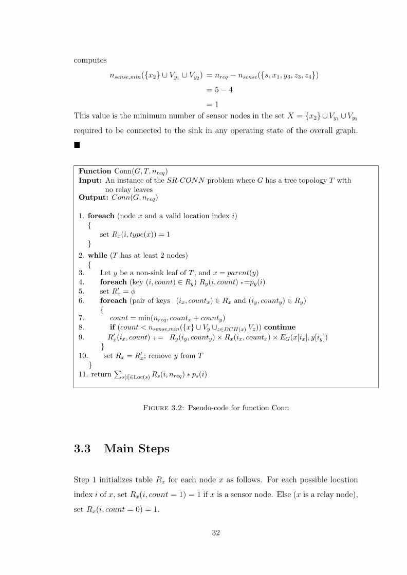
Function Conn(G,T, nreq)Input: An instance of the SR-CONN problem where G has a tree topology T with

no relay leavesOutput: Conn(G,nreq)

1. foreach (node x and a valid location index i){

set Rx(i, type(x)) = 1}

2. while (T has at least 2 nodes){

3. Let y be a non-sink leaf of T , and x = parent(y)4. foreach (key (i, count) ∈ Ry) Ry(i, count) ∗=py(i)5. set R′x = φ6. foreach (pair of keys (ix, countx) ∈ Rx and (iy, county) ∈ Ry)

{7. count = min(nreq, countx + county)8. if (count < nsense,min({x} ∪ Vy ∪z∈DCH(x) Vz)) continue

9. R′x(ix, count) += Ry(iy, county)×Rx(ix, countx)× EG(x[ix], y[iy])}

10. set Rx = R′x; remove y from T}

11. return∑

s[i]∈Loc(s)Rs(i, nreq) ∗ ps(i)

Figure 3.2: Pseudo-code for function Conn

3.3 Main Steps

Step 1 initializes table Rx for each node x as follows. For each possible location

index i of x, set Rx(i, count = 1) = 1 if x is a sensor node. Else (x is a relay node),

set Rx(i, count = 0) = 1.

32

Steps 2-10 form the main loop of the function. The loop iteratively finds a leaf

node y that is not the sink s, processes node y, and then removes y from the tree

T . Processing a node y with parent x is done as follows.

Step 4 updates each entry Ry(i, count) by multiplying the entry with py(i). As

can be seen, this update operation is done in the iteration that ends by removing

y. Step 5 initializes the temporary table R′x to empty.

Steps 6-9: the loop in Step 6 performs a cross product of tables Rx and Ry,

storing the result in table R′x. In the cross product, each pair of possible keys

(ix, countx) and (iy, county) are processed. More specifically, suppose that x[ix]

can reach countx sensor nodes in the part of Tx processed thus far with probability

Rx(ix, countx). Also, suppose that y[iy] can reach county sensor nodes in Ty with

probability Ry(iy, county). Thus, if x[ix] reaches y[iy] (i.e., EG(x[ix], y[iy])= 1)

then x[ix] can reach a total of count = countx + county nodes.

If count > nreq then Step 7 truncates count to nreq. On the other hand, if count <

nsense,min({x}∪Vy∪z∈DCH(x)Vz) (i.e., count is below the minimum number of nodes

required to construct an operating state) then Step 8 skips Step 9 and starts a

new iteration. Step 9 updates the probabilities accumulated in R′x(ix, count).

After exiting the main loop, the current tree T contains only the sink node s. Step

11 computes the solution Conn(G, nreq) from the table Rs associated with the sink

s.

3.4 Correctness

To prove correctness, we first introduce the following notation and definitions. For

a given node x, and iteration r ∈ [1, n− 1] of the main loop in Step 2, we have the

following:

• DCH(x, r): The set of x’s deleted children at the start of iteration r.

33

• Vx,deleted,r (=⋃y∈DCH(x,r) Vy): The set of x’s deleted descendants at the start

of iteration r.

For brevity, we omit r when the iteration number is not important, or understood

by the context.

In the following definitions, x is any node in T , i is a possible location index of

x, and Vx,delete is the set of deleted descendants associated with x at the start of

some iteration.

[D1] Let S be a state over nodes in {x}⋃Vx,delete. The type of S is a pair (i, count)

where

• x is at location x[i]

• If count = nreq then the number of sensor nodes connected to x[i] in S

is ≥ nreq

• Else (count < nreq), then the number of sensor nodes connected to x[i]

is < nreq

[D2] We say that table Rx is complete with respect to a given set Vx,delete if the

following conditions hold:

(a) For each key (i, count) in Rx, Rx(i, count) is the probability of obtaining

states over {x[i]}⋃Vx,delete of type (i, count). (Before multiplying by

px(i), the probability is conditioned on x being at location x[i]).

(b) Each key (i, count) not in Rx does not contribute to computing the

solution Conn(G, nreq).

We now show the following theorem.

Theorem 3.1. At the start of each iteration of the main loop in Step 2, if x is a

node in the current tree T then table Rx is complete with respect to the associated

set Vx,delete of deleted nodes.

34

Proof.

Loop initialization: At the start of the 1st iteration, T contains all nodes V ,

and each node x has Vx,delete = ∅. Node x in location x[ix] is associated with one

state of type (ix, countx = 0) if x is a relay node, or type (ix, countx = 1) if x is a

sensor node. For each such state type, Step 1 correctly sets Rx(i, count).

Loop maintenance: Assume the theorem holds for all possible iterations r,

where r ≤ n− 2. We show that it holds in iteration r + 1. Let y be the leaf node

deleted in iteration r, and x = parent(y). Rx is the only relevant table that may

have changed between iterations r and r+ 1 (table Ry is also changed but node y

is deleted at the end of the iteration). Thus, it suffices to show that Rx is complete

with respect to {x}⋃Vx,delete,r+1 at the start of iteration r + 1. To this end, we

note the following in iteration r:

• Step 4: this step adjusts the probability of each state type (i, count) in Ry

by taking into account py(i).

• Step 6: this loop exhaustively generates all state types over the set Vy⋃Vx,delete,r

where Vy is all nodes of the subtree rooted at node y.

• Step 8: this step discards all state types that can not be extended (by

adding sensor nodes from the unprocessed part of the tree) to satisfy the

nreq requirement.

• Step 9: this step updates the probability of R′x(ix, count) by adding the right

hand side when states of type (ix, count) can be extended to operating states.

�

Following an argument similar to the loop maintenance argument, one can show

that at Step 11, table Rs associated with the sink node is complete with respect

to all nodes V in the network. Thus, the function returns the required solution

Conn(G, nreq).

35

3.5 Running Time

Let n be the number of nodes in G, and `max be the maximum number of locations

in the locality set of any node.

Theorem 3.2. Function Conn solves the SR-CONN problem in O(n · n2req · `2max)

time

Proof. We note the following.

• Step 1: storing the tree T requires O(n) time.

• Step 2: the main loop performs n− 1 iterations. Each of Steps 3, 5, and 10

can be done in constant time.

• Step 4: this loop requires O(nreq · `max) time.

• Step 6: this loop requires O(n2req · `2max) iterations. Steps 7, 8, and 9 can be

done in constant time.

Thus, the overall running time is determined by the main loop that requires

O(n · n2req · `2max) time. �

Theorem 3.3. Function Conn solves the AR-CONN problem in O(n · `2max) time.

Proof. It suffices to show that the main loop requires the above time. In the

AR-CONN problem, nreq = |Vsense|, and all sensor nodes in any subtree Ty should

be connected to the root y in any operating state. So, in any iteration of the

main loop, each table Ry contains keys (i, count) for only one value of count (the

maximum value obtainable from descendants of y processed and removed thus

far). That is, the maximum length of any table is `max independent of nreq. This

gives the running time shown in the theorem. �

36

3.6 Simulation Results

We present performance results of the algorithm with results on partial 2-trees and

3-trees in the next chapter. The tree algorithm is empirically fast. The running

time is typically less than 50 millisecond for the tested tree networks of size ≤ 20

nodes. In contrast, the algorithm for 2-trees and 3-trees may require time in the

order of minutes to solve a network with 15 nodes.

3.7 Concluding Remarks

Quantifying the likelihood that a sufficient number of sensor nodes is connected

to a sink node in a given UWSN is a challenging problem for networks with semi-

mobile and mobile nodes. Here, we adopt a flexible probabilistic graph model to

formulate a class of parametrized network connectivity problems. The problem

setting allows the network to utilize both sensor nodes and relay nodes. For

scenarios where the model is exact, our devised algorithm shows that the exact

probabilistic connectivity can be computed efficiently for tree-like networks.

37

Chapter 4

The A-CONN Problem on Partial

k-trees

In this chapter, we present a dynamic programming algorithm to solve

theA-CONN problem on a probabilistic input graphG = (V,EG, Loc, p)

that is known a priori to have the topology of a partial k-tree, for

some specified k. The algorithm takes as input a perfect elimination

sequence (PES) of the partial k-tree. The devised algorithm is exact

for the given probabilistic graph, and runs in polynomial time, for any

fixed k. We present simulation results that illustrate some aspects of

the algorithm’s performance and use.

4.1 Overview of the Algorithm

In this section, we outline the main ingredients of our devised dynamic pro-

gramming algorithm to solve the A-CONN problem on partial k-trees. Similar

to the previous chapter, we model the given UWSN as a probabilistic network

G = (V,EG, Loc, p) where V = Vsense (i.e., the network has no relay nodes).

We assume that the probabilistic graph G has the topology of a partial k-tree for

some specified k. Recall, for any two sensor nodes x and y in Vsense with possible

38

positions x[i] ∈ Loc(x) and y[j] ∈ Loc(y) if EG(x[i], y[j]) = 1 then (x, y) is an edge

of the underlying partial k-tree.

In addition, we need the following notation:

• For simplicity, and when no confusion can arise, we use G to refer also to

the partial k-tree graph underlying the structure of the given probabilistic

network.

• We denote by G a complete k-tree of whichG is a subgraph (i.e., a completion

of G to a k-tree) such that the given PES applies to G.

To explain the structure of the algorithm, we introduce below the following con-

cepts.

• The node processing order used in the algorithm

• The concept of reducing a subgraph onto a separator clique

• The concept of network state types used in the algorithm

• The structure of the tables used to store the states of the dynamic program

The algorithm processes the nodes in the order of the given PES, say PES =

(v1, v2, . . . , vn−k) where the last node vn = s (the sink node). To explain the

processing done on node vi, we introduce the following notation. We use the

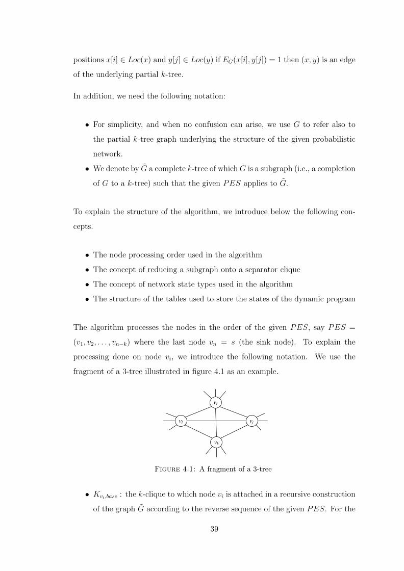
fragment of a 3-tree illustrated in figure 4.1 as an example.

 

vi

vl

vk

vj

Figure 4.1: A fragment of a 3-tree

• Kvi,base : the k-clique to which node vi is attached in a recursive construction

of the graph G according to the reverse sequence of the given PES. For the

39

3-tree fragment in figure 4.1, assume that Kvi,base is the triangle (3-clique)

on nodes {vj, vk, vl}.• Kvi,1, Kvi,2, . . . , Kvi,k : all possible k-cliques involving node vi when this node

becomes a k-leaf, assuming that we started with the full k-tree G. Each k-

clique is made of node vi and k − 1 nodes in Kvi,base. For the 3-tree in

figure 4.1, we may set Kvi,1 = the triangle (vi, vj, vk), Kvi,2 = the triangle

(vi, vj, vl), Kvi,3 = the triangle (vi, vk, vl).

Processing of node vi is done when all nodes in the prefix v1, v2, . . . , vi−1 have been

processed and deleted, and thus node vi becomes a k-leaf (also called a simplicial

node) in the current reduced graph. Information about certain subgraphs on

the deleted nodes are maintained in special tables associated with the k-cliques

Kvi,base, Kvi,1, . . . , Kvi,k. We use Tvi,α to denote the table associated with clique

Kvi,α where α = base, 1, 2, . . . , k.

Example 4.1. In figure 4.2, if va and vb have been deleted to make vi a simplicial

node, the information about the induced subgraph on nodes (va, vb, vi, vj, vk) is

summarized in table, say, Tvi,1 associated with clique Kvi,1 = (vi, vj, vk). �

 

vi

vl

vk

vj

va

vb

Figure 4.2: A 3-tree fragment

In the above example, we say that the induced subgraph on nodes (va, vb, vi, vj, vk)

is reduced onto the clique (vi, vj, vk). Thus, prior to processing node vi, the al-

gorithm maintains in each table Tvi,α (where α = base, 1, 2, . . . , k) information

about a subgraph, denoted Gvi,α, that has been reduced onto the clique Kvi,α.

Initially, each such table Tvi,α stores information about the k-clique Kvi,α itself.

More specifically, the algorithm stores information about some useful network

states of the graph Gvi,α in the table Tvi,α.

40

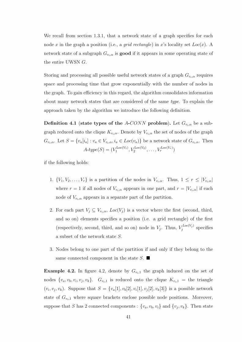
We recall from section 1.3.1, that a network state of a graph specifies for each

node x in the graph a position (i.e., a grid rectangle) in x’s locality set Loc(x). A

network state of a subgraph Gvi,α is good if it appears in some operating state of

the entire UWSN G.

Storing and processing all possible useful network states of a graph Gvi,α requires

space and processing time that grow exponentially with the number of nodes in

the graph. To gain efficiency in this regard, the algorithm consolidates information

about many network states that are considered of the same type. To explain the

approach taken by the algorithm we introduce the following definition.

Definition 4.1 (state types of the A-CONN problem). Let Gvi,α be a sub-

graph reduced onto the clique Kvi,α. Denote by Vvi,α the set of nodes of the graph

Gvi,α. Let S = {va[ia] : va ∈ Vvi,α, ia ∈ Loc(va)} be a network state of Gvi,α. Then

A-type(S) = (VLoc(V1)1 , V

Loc(V2)2 , . . . , V

Loc(Vr)r )

if the following holds:

1. {V1, V2, . . . , Vr} is a partition of the nodes in Vvi,α. Thus, 1 ≤ r ≤ |Vvi,α|where r = 1 if all nodes of Vvi,α appears in one part, and r = |Vvi,α| if each

node of Vvi,α appears in a separate part of the partition.

2. For each part Vj ⊆ Vvi,α, Loc(Vj) is a vector where the first (second, third,

and so on) elements specifies a position (i.e. a grid rectangle) of the first

(respectively, second, third, and so on) node in Vj. Thus, VLoc(Vj)j specifies

a subset of the network state S.

3. Nodes belong to one part of the partition if and only if they belong to the

same connected component in the state S. �

Example 4.2. In figure 4.2, denote by Gvi,1 the graph induced on the set of

nodes {va, vb, vi, vj, vk}. Gvi,1 is reduced onto the clique Kvi,1 = the triangle

(vi, vj, vk). Suppose that S = {va[1], vb[2], vi[1], vj[2], vk[3]} is a possible network

state of Gvi,1 where square brackets enclose possible node positions. Moreover,

suppose that S has 2 connected components : {va, vb, vi} and {vj, vk}. Then state

41

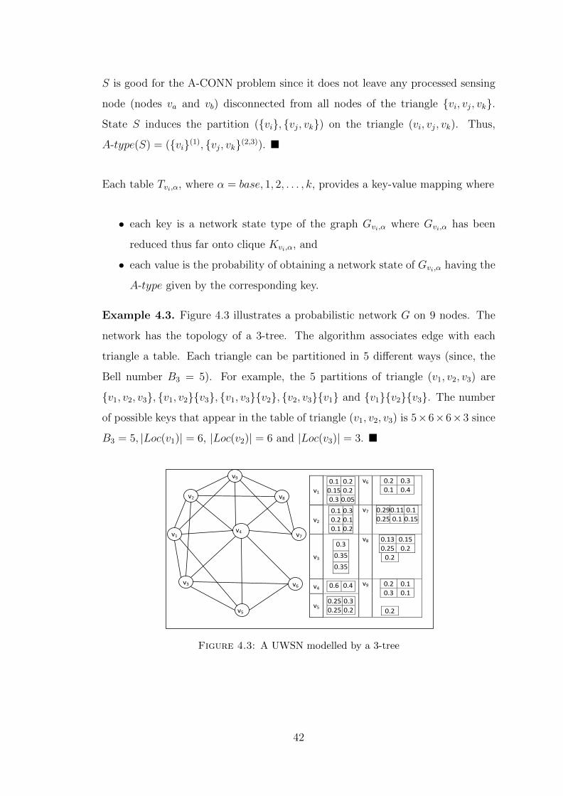
S is good for the A-CONN problem since it does not leave any processed sensing

node (nodes va and vb) disconnected from all nodes of the triangle {vi, vj, vk}.State S induces the partition ({vi}, {vj, vk}) on the triangle (vi, vj, vk). Thus,

A-type(S) = ({vi}(1), {vj, vk}(2,3)). �

Each table Tvi,α, where α = base, 1, 2, . . . , k, provides a key-value mapping where

• each key is a network state type of the graph Gvi,α where Gvi,α has been

reduced thus far onto clique Kvi,α, and

• each value is the probability of obtaining a network state of Gvi,α having the

A-type given by the corresponding key.

Example 4.3. Figure 4.3 illustrates a probabilistic network G on 9 nodes. The

network has the topology of a 3-tree. The algorithm associates edge with each

triangle a table. Each triangle can be partitioned in 5 different ways (since, the

Bell number B3 = 5). For example, the 5 partitions of triangle (v1, v2, v3) are

{v1, v2, v3}, {v1, v2}{v3}, {v1, v3}{v2}, {v2, v3}{v1} and {v1}{v2}{v3}. The number

of possible keys that appear in the table of triangle (v1, v2, v3) is 5×6×6×3 since

B3 = 5, |Loc(v1)| = 6, |Loc(v2)| = 6 and |Loc(v3)| = 3. �

 

 

   

 

 

v10.1 0.20.15 0.20.3 0.05

 

v6 0.2 0.30.1 0.4

 

v20.1 0.30.2 0.10.1 0.2

 

v7 0.290.11 0.1 0.25 0.1 0.15

 

v3

0.3

0.35

0.35 

v8 0.13 0.150.25 0.2 0.2

 

v4 0.6 0.4 

v9 0.2 0.10.3 0.1

 0.2

 

v50.25 0.30.25 0.2

 

v4 

 v9 

 v1  v7

v5

 v2   v8 

v6 v3 

Figure 4.3: A UWSN modelled by a 3-tree

42

4.2 Algorithm Organization

The overall algorithm is organized around 3 functions : a top level main function

(Algorithm 1), a middle level table merge function (Algorithm 2: t merge), and a

low level partition merge function (Algorithm 3: p merge).

The highlights of each function are explained below:

• Function Main (Algorithm 1): This function reduces the structure of the

probabilistic network (and the underlying partial k-tree)G by iteratively pro-

cessing and then deleting nodes according to the given PES, say (v1, v2, . . . , vn)

where Vn = s (the sink node), until the network is reduced to the k-

clique (vn−k+1, . . . , vn). Processing a node vi entails merging the tables

{Kvi,α : α = base, 1, 2, . . . , k}. This merging phase is done by merging a

sequence of pairs of tables. The middle level table merge function is used

for this purpose. After all iterations are done, the solution is computed from

the table associated with the clique on nodes (vn−k+1, . . . , vn).

• Function Table Merge (Algorithm 2: t merge): This function takes as input

a pair of tables, denoted T1 and T2, associated with two overlapping cliques.

Roughly speaking, it performs a cross-product of T1 and T2; that is, it con-

structs a new table, denoted Tout, by processing every pair of keys: key1 ∈ T1and key2 ∈ T2. To process the partition parts of the keys P1 ∈ key1 and

P2 ∈ key2, the function calls the low level partition merge function.

• Function Partition Merge (Algorithm 3: p merge): This function takes two

partitions P1 ∈ key1 ∈ T1 and P2 ∈ key2 ∈ T2, as explained above, and

computes a partition Pout that is a valid partition of a key in the merged

table T .

43

4.2.1 Function Main

Algorithm 1 presents the main steps of the top level main function. The algorithm

takes as input a probabilistic network G = (V,EG, Loc, p) that has the topology of

a partial k-tree, also denoted G, and a PES of G. It computes the exact A-CONN

of G in Conn(G). For simplicity of presenting the pseudo-code, we assume that

the nodes V = Vsense in G are labelled so that the PES = (v1, v2, . . . , vn) and

vn = s (the sink node).

The function has 3 main parts, as explained below.

Initialization (Step 1): We initialize a table TH associated with each k-clique H

in the full k-tree G. In particular, for each possible state type, say k, of a network

state on the nodes of H, we set a key-value entry in TH where the key is k, and the

value is the probability of obtaining a network state of H of that type. If G is a

strict partial k-tree (So, G 6= G ) then some edges of H may be missing. However,

the above initialization approach is still applicable.

We remark that initializing table TH for a k-clique H can be done as follows.

1. First, we construct for each edge e = {x, y} in H an exhaustive table Te.

As explained above, Te contains key-value mappings. Each key has the form

A-type(S) for a possible state S on {x, y} (e.g., ({x}(1){y}(1)), {x, y}(1,1), . . .).The value associated with A-type(S) is the probability of obtaining a network

state of this A-type over the edge e.

2. Second, we compute (using function t merge and p merge) the cross product

of all tables associated with all edges in the k-clique H.

Main Loop (Step 2): The main loop has two parts. The first part (Steps 2

to 6) iteratively processes and deletes nodes in the PES. Processing a node vi

entails merging a sequence of tables (Tvi,α : α = base, 1, 2, . . . , k) into one table.

This step is carried by merging a pair of tables at a time. We use table Temp to

store intermediate results. We store the final result in table Tvi,base.

44

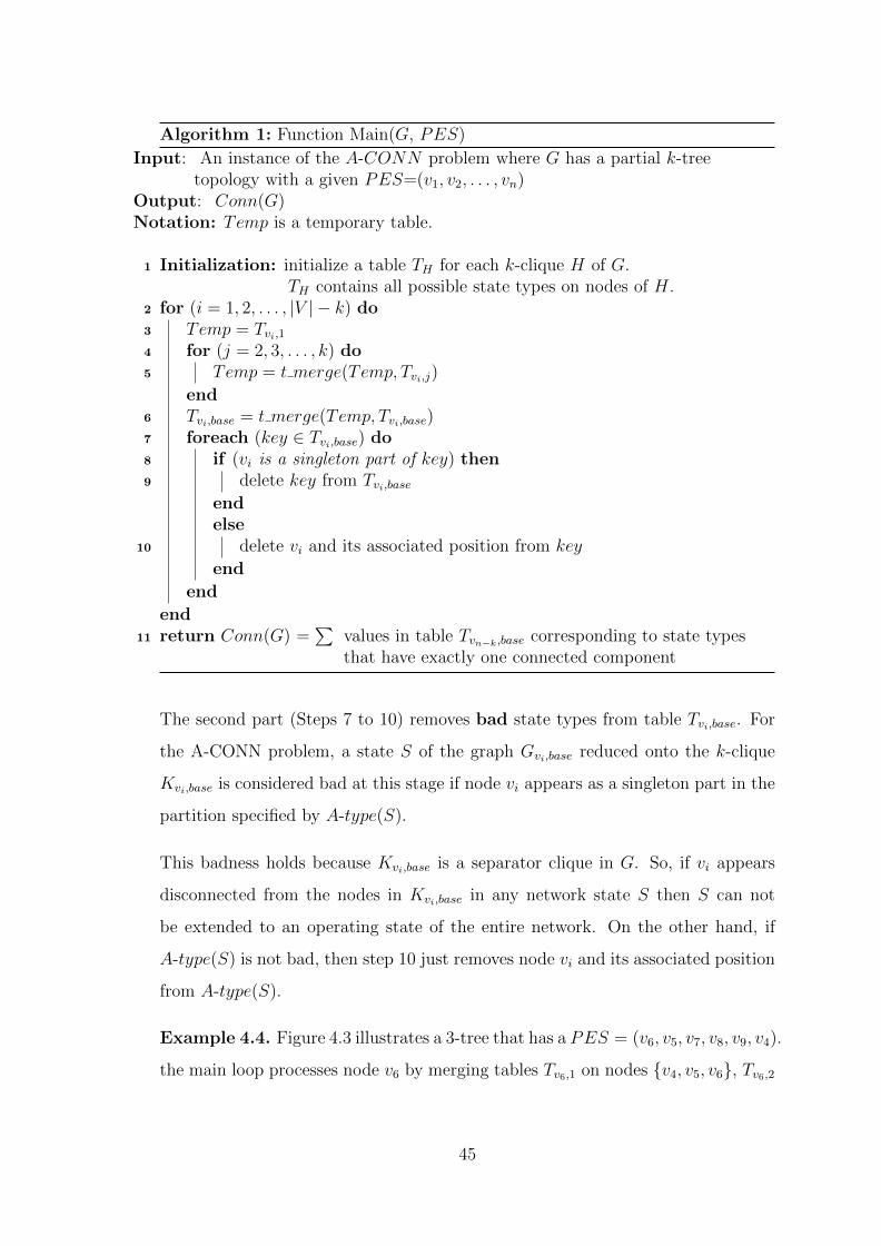
Algorithm 1: Function Main(G, PES)

Input: An instance of the A-CONN problem where G has a partial k-treetopology with a given PES=(v1, v2, . . . , vn)

Output: Conn(G)Notation: Temp is a temporary table.

1 Initialization: initialize a table TH for each k-clique H of G.TH contains all possible state types on nodes of H.

2 for (i = 1, 2, . . . , |V | − k) do3 Temp = Tvi,14 for (j = 2, 3, . . . , k) do5 Temp = t merge(Temp, Tvi,j)

end6 Tvi,base = t merge(Temp, Tvi,base)7 foreach (key ∈ Tvi,base) do8 if (vi is a singleton part of key) then9 delete key from Tvi,base

endelse

10 delete vi and its associated position from key

end

end

end11 return Conn(G) =

∑values in table Tvn−k,base corresponding to state typesthat have exactly one connected component

The second part (Steps 7 to 10) removes bad state types from table Tvi,base. For

the A-CONN problem, a state S of the graph Gvi,base reduced onto the k-clique

Kvi,base is considered bad at this stage if node vi appears as a singleton part in the

partition specified by A-type(S).

This badness holds because Kvi,base is a separator clique in G. So, if vi appears

disconnected from the nodes in Kvi,base in any network state S then S can not

be extended to an operating state of the entire network. On the other hand, if

A-type(S) is not bad, then step 10 just removes node vi and its associated position

from A-type(S).

Example 4.4. Figure 4.3 illustrates a 3-tree that has a PES = (v6, v5, v7, v8, v9, v4).

the main loop processes node v6 by merging tables Tv6,1 on nodes {v4, v5, v6}, Tv6,2

45

on nodes {v3, v5, v6}, Tv6,3 on nodes {v3, v4, v6}, and Tv6,base on nodes {v3, v4, v5}into one table stored in Tvi,base. �

Termination (Step 11): The main loop finishes after processing node vn−k. The

resulting table Tvn−k,base corresponds to the k-clique H on nodes (vn−k+1, . . . , vn).

Any state type where all nodes of H appear in one connected component corre-

sponds to a set of operating network states of the entire network . Thus, we return

the sum of probabilities of all such state types.

4.2.2 Function Table Merge

Algorithm 2: Function t merge(T1, T2)

Input: Two tables T1 and T2 that may share common nodesOutput: A merged table Tout

1 Initialization: Clear table Tout2 set C = the set of common nodes between T1 and T23 foreach (pair of state types key1 ∈ T1 and key2 ∈ T2) do4 if (any node in C lies in two different positions in key1 and key2) then5 continue

end6 set keyout = the state type obtained from node positions in key1 and key2,

and the partition computed by p merge(key1, key2)7 set pout = T1(key1)× T2(key2) adjusted to take the effect of common nodes in

C into consideration8 if (keyout ∈ Tout) then9 update Tout(kout) +=pout

endelse

10 set Tout(keyout) = poutend

end11 return Tout

Algorithm 2 illustrates the main steps of the middle level table merge function. We

recall that t merge is called from the main function to merge two tables, denoted

T1 and T2, that may have a set C of common nodes (i.e., V (T1) ∩ V (T2) 6= ∅).Each table Ti, i = 1, 2, stores information about some subgraph, Gi, that has been

46

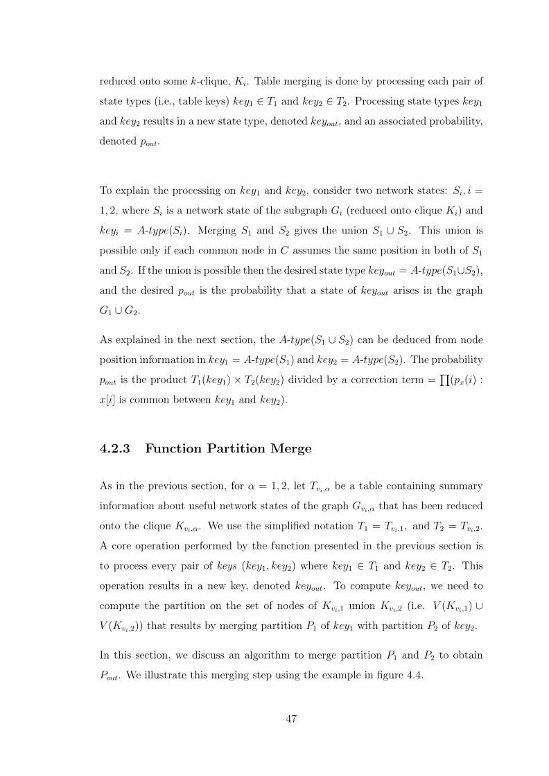
reduced onto some k-clique, Ki. Table merging is done by processing each pair of

state types (i.e., table keys) key1 ∈ T1 and key2 ∈ T2. Processing state types key1

and key2 results in a new state type, denoted keyout, and an associated probability,

denoted pout.

To explain the processing on key1 and key2, consider two network states: Si, i =

1, 2, where Si is a network state of the subgraph Gi (reduced onto clique Ki) and

keyi = A-type(Si). Merging S1 and S2 gives the union S1 ∪ S2. This union is

possible only if each common node in C assumes the same position in both of S1

and S2. If the union is possible then the desired state type keyout = A-type(S1∪S2),

and the desired pout is the probability that a state of keyout arises in the graph

G1 ∪G2.

As explained in the next section, the A-type(S1 ∪ S2) can be deduced from node

position information in key1 = A-type(S1) and key2 = A-type(S2). The probability

pout is the product T1(key1) × T2(key2) divided by a correction term =∏

(px(i) :

x[i] is common between key1 and key2).

4.2.3 Function Partition Merge

As in the previous section, for α = 1, 2, let Tvi,α be a table containing summary

information about useful network states of the graph Gvi,α that has been reduced

onto the clique Kvi,α. We use the simplified notation T1 = Tvi,1, and T2 = Tvi,2.

A core operation performed by the function presented in the previous section is

to process every pair of keys (key1, key2) where key1 ∈ T1 and key2 ∈ T2. This

operation results in a new key, denoted keyout. To compute keyout, we need to

compute the partition on the set of nodes of Kvi,1 union Kvi,2 (i.e. V (Kvi,1) ∪V (Kvi,2)) that results by merging partition P1 of key1 with partition P2 of key2.

In this section, we discuss an algorithm to merge partition P1 and P2 to obtain

Pout. We illustrate this merging step using the example in figure 4.4.

47

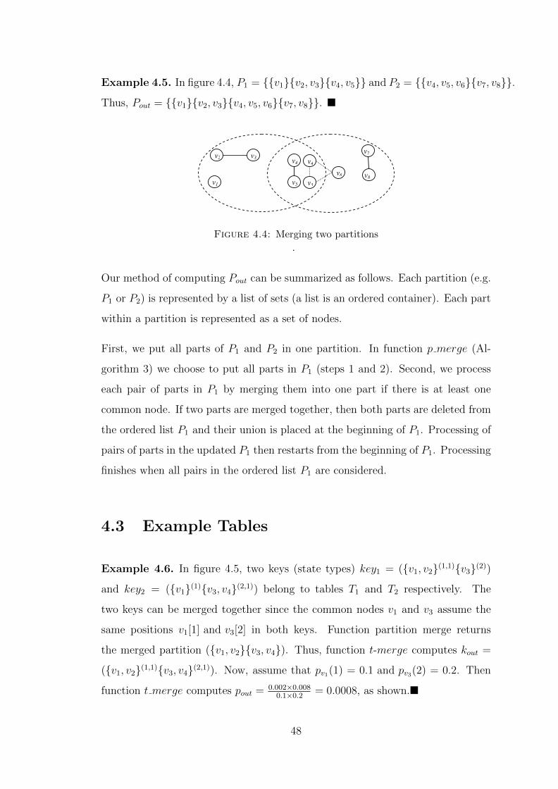
Example 4.5. In figure 4.4, P1 = {{v1}{v2, v3}{v4, v5}} and P2 = {{v4, v5, v6}{v7, v8}}.Thus, Pout = {{v1}{v2, v3}{v4, v5, v6}{v7, v8}}. �

 

v4v2

v5

v3

v1

v4

v5

v6

v7

v8

Figure 4.4: Merging two partitions

.

Our method of computing Pout can be summarized as follows. Each partition (e.g.

P1 or P2) is represented by a list of sets (a list is an ordered container). Each part

within a partition is represented as a set of nodes.

First, we put all parts of P1 and P2 in one partition. In function p merge (Al-

gorithm 3) we choose to put all parts in P1 (steps 1 and 2). Second, we process

each pair of parts in P1 by merging them into one part if there is at least one

common node. If two parts are merged together, then both parts are deleted from

the ordered list P1 and their union is placed at the beginning of P1. Processing of

pairs of parts in the updated P1 then restarts from the beginning of P1. Processing

finishes when all pairs in the ordered list P1 are considered.

4.3 Example Tables

Example 4.6. In figure 4.5, two keys (state types) key1 = ({v1, v2}(1,1){v3}(2))and key2 = ({v1}(1){v3, v4}(2,1)) belong to tables T1 and T2 respectively. The

two keys can be merged together since the common nodes v1 and v3 assume the

same positions v1[1] and v3[2] in both keys. Function partition merge returns

the merged partition ({v1, v2}{v3, v4}). Thus, function t-merge computes kout =

({v1, v2}(1,1){v3, v4}(2,1)). Now, assume that pv1(1) = 0.1 and pv3(2) = 0.2. Then

function t merge computes pout = 0.002×0.0080.1×0.2 = 0.0008, as shown.�

48

Algorithm 3: function p merge(P1, P2)

Input: Two partitions P1 and P2

Output: A partition PNotation: s and t are two set iterators and their corresponding set areindicated by s∗ and t∗.

1 foreach ( set s∗ in P2) do2 P1.push back(s∗)

end3 for (s = P1.begin(); s 6= P1.end(); + + s) do4 for (t = s.next(); t 6= P1.end(); + + t) do5 if (s∗ ∩ t∗ 6= ∅) then6 P1.push front(s

∗ ∪ t∗)7 P1.delete(s

∗)8 P1.delete(t

∗)9 s = P1.begin()

10 break

end

end

end11 set P = P1

return P

kout = type(S1 ∪ S2), and the desired pout is the probability that a state of type

kout arises in the graph G1 ∪G2.

As explained in the next section, the type(S1 ∪ S2) can be deduced from the

node position information in k1 = type(S1) and k2 = type(S2). The probabil-

ity pout is the product T1(k1) × T2(k2) divided by a correction term =∏

(p(i)x :

x[i] is common between k1 and k2).

T1 on (v1, v2, v3). .

{v1, v2}(1,1){v3}(2) 0.002. .. .. .

×

T2 on (v1, v3, v4). .

{v1}(1){v3, v4}(2,1) 0.008. .. .. .

⇒Temp on (v1, v2, v3, v4)

. .

{v1, v2}(1,1){v3, v4}(2,1) 0.0008. .. .. .

Table 4.1: Merging two tables

Temp on (v1, v2, v3, v4). .

{v1, v2}(1,1){v3, v4}(2,1) 0.0008. .. .. .

⇒Temp on (v2, v3, v4)

. .

{v2}(1){v3, v4}(2,1) 0.0008. .. .. .

Table 4.2: Deleting node v1

Example 4.5. Table 4.4 illustrates merging row {v1, v2}{1,1}{v3}{2} 0.002 of table

T1 with row {v1}{1}{v3, v4}{2,1} 0.008 of table T2 which is fundamental operation

for merging two tables. The function merge uses pMerge function which takes

two partitions {v1, v2}{v3} and {v1}{v3, v4} and returned {v1, v2}{v3, v4}. The

partition {v1} merge with partition {v1, v2} because there is a common node v1

between these two partition. So after merging the result will be {v1, v2} ∪ {v1} =

{v1, v2}. {v1} is not going to merge with {v3, v4} because there is no common

nodes between these two partition. Similarly partition {v3} merge with partition

{v3, v4} and the result is {v3, v4}. The merge function updates the locality set

of each node of the merged partition {v1, v2}{1,1}{v3, v4}{2,1} from the locality set

of nodes in merging partitions. There are two common nodes v1 and v3 located

in region 1 and 2 respectively with probability 0.1 and 0.2 respectively in the

merging partitions. It update the probability of newly created partition 0.0008 by

multiplying row-wise probabilities 0.002 × 0.008 and dividing the probability by

product of the common nodes corresponding regional probabilities 0.1× 0.2.

Table ?? shows the deletion of node v1 from Temp. The function main simply

look for the node and remove it and it’s locality set from key.�

40

Figure 4.5: Merging two tables

.

Example 4.7. Figure 4.6 illustrates the operation of the second part of the main

loop of function Main in the iteration where node v1 is processed. The table

on the left represents Tvi,base after the first part of the main loop finishes. Key

{v1, v2}(1,1){v3, v4}(2,1) is good in Tvi,base since v1 is connected to v2 in any network

state of this type. Hence, node v1 and its associated position can be deleted from

the key. The reduced key appears in the updated Tvi,base on the right.

49

Tv1,base on (v1, v2, v3, v4). .

{v1, v2}(1,1){v3, v4}(2,1) 0.0008. .. .. .

⇒Tv1,base on (v2, v3, v4)

. .

{v2}(1){v3, v4}(2,1) 0.0008. .. .. .

Table 1: Deleting node v1 from Temp

1

Figure 4.6: Deleting node vi.

4.4 Correctness

To prove correctness, we introduce the following notation and definitions.

[D1] We say that a table Tvi,α is complete with respect to a graph Gvi,α that has

been reduced onto the clique Kvi,α if the following conditions hold:

a) For each key ∈ Tvi,α, the corresponding value Tvi,α(key) is the proba-

bility of obtaining states over the subgraph Gvi,α of type key.

b) Each key not in Tvi,α does not contribute to computing the solution

Conn(G).

We now show the following theorem.

Theorem 4.2. At the start of each iteration of the main loop (Step 2) of func-

tion Main, if vi is a node in the current graph then each table Tvi,α : α =

1, 2, . . . , k, base, is complete with respect to the graph Gvi,α reduced thus far onto

the clique Kvi,α.

Proof.

Loop Initialization: At the start of the first iteration, G contains all nodes V .

In addition, for each clique Kvi,α, the subgraph Gvi,α reduced thus far onto the

clique Kvi,α is the clique itself (as done in Step 1 of function Main).

50

Loop Maintenance: Assume the theorem holds for all possible iterations r,

where r ≤ n − k − 1. We show that it holds in iteration r + 1. Let vr be the

k-leaf deleted in iteration r. Table Tvr,base is the only table that may have changed

between iterations r and r + 1. Thus, it suffices to show that Tvr,base is complete

with respect to Gvr,base. To this end, we note the following in iteration r:

• Steps 3 to 6 of function Main merge all tables in the set {Tvi,α : α =

1, 2, . . . , k, base} into Tvi,base.

• The loop in Step 7 of function Main discards all bad state types over the

graph⋃

α∈{1,2,...,k,base}Gvi,α. �

Following an argument similar to the loop maintenance argument, one can show

that at Step 11 in function Main, table Tvn−k,base associated with the clique Tvn−k,base

containing the sink node is complete with respect to all nodes V . Thus, the func-

tion returns the required solution.

4.5 Running time

Let n be the number of nodes in G, lmax be the maximum number of locations in

the locality set of any node, and Bk be the kth Bell number.

Theorem 4.3. In the A-CONN algorithm we have

1. The maximum length of any table is ∈ O(Bklkmax).

2. The worst case running time is O(n(Bklkmax)

2).

Proof.

To see (1), we note that the length of each table is determined by the number of

partitions of any set of k nodes (= Bk) times the number of different positions

that the k nodes can take (∈ O(lkmax)). Thus, the maximum length of any table is

51

O(Bklkmax).

To see (2), we note that function t merge processes O((Bklkmax)

2) pairs of keys in

each call. Function partition merge takes O(k3) to merge two partitions; this is a

constant time for any fixed k. Thus, merging two tables requires O((Bklkmax)

2).

Function Main processes each node by merging a set of k+1 tables. This is done

by calling function t merge k times. Thus, function Main processes each node in

O(k(Bklkmax)

2). Since k is a constant, processing each node requires O((Bklkmax)

2).

The answer is obtained after processing n-k nodes. Thus, the overall running time

is O(n(Bklkmax)

2). �

4.6 Software Verification

Our devised dynamic programming algorithm is implemented in the C++ lan-

guage with the use of STL (Standard Template Library) container classes. The

program has about 1,300 executable lines (including debugging code). To check

the correctness of the implementation, we used the following approaches.

1. For probabilistic networks with small number of network states (e.g., ≤ 32

states) we compare the program output with manual calculations.

2. By definition, if every possible network state is connected then Conn(G) = 1

regardless of node locations and probability distributions. We verified the

output of the program for networks that are manually designed to satisfy

this property.

3. Consider two probabilistic networks Gx and Gy where

• Conn(Gx) = Conn(Gy) = 1, and

• x and y are distinguished nodes in Gx and Gy respectively.

Now, consider the network G obtained from Gx and Gy by introducing a link

(x[i], y[j]) for some positions of node x and node y. No other node in Gx

can reach another node in Gy. Let p(x, y) be the probability that link (x, y)

52

arises. Then Conn(G) = p(x, y). We utilize the above approach to check

correctness.

4. If G1, G2, and G3 are a tree, 2-tree, and 3-tree graphs where G1 ⊂ G2 ⊂G3. Then Conn(G1) ≤ Conn(G2) ≤ Conn(G3). Relations of this type are

checked in all of the obtained results.

5. For any probabilistic network G, using different PESs should result in com-

puting the same Conn(G) value. We used the above property to check our

implementation.

4.7 Simulation Results

In this section we present simulation results that explore the following performance

aspects of our devised algorithm:

1. Execution time of the algorithm

2. Effect of increasing the parameter k

3. Effect of increasing node transmission range

4. Effect of k-tree subgraph selection method

 

v1 0.2 0.5 0.10.150.05

v6 0.6 0.2 0.1 0.1

v2 0.25 0.3 0.16 0.29 v7 0.5 0.25 0.2

v3 0.2 0.3 0.10.1 0.15 0.15 v8

0.25 0.360.14 0.25

v4 0.25 0.350.25 0.15 v9 0.7 0.15 0.15

v5 0.16 0.18 0.140.3 0.22 v10

0.18 0.24 0.34 0.1 0.14

v8 v10 

 v1 

v7

 v9 

 v6  v5 

 v4 

 v2 

v3

1‐tree   

2‐tree   

3‐tree   

Figure 4.7: Network G10

Test Networks: For simplicity of constructing test networks and analyzing the

obtained results, we assume that all nodes have the same transmission range Rtr,

53

 

 

   

 

 

v1 0.2 0.3 0.15 .050.07 0.15 0.05 0.03

v7 0.1 0.22 .14

.02 .14

v2 0.33 0.37 0.3 .12

v8 0.4 0.3

v3 0.25 0.2 0.15 0.12

v9 0.3 0.2 0.5

v4 0.3 0.22 0.31 0.1

v10 0.34 0.13 0.13 0.1 0.3

v5 0.3 0.16 0.24 0.3

v11 0.2 0.5 0.3

v6 0.5 0.3 0.15

v12 0.1 0.2 0.10.13 0.20.07 0.12 0.8

 

1‐tree   

2‐tree   

3‐tree   

v8v11

 v1 V10

v7

v9

 v6 v5 

 v4 

 v2 

 v3 

v12

Figure 4.8: Network G12

and we set the EG relation according to the Euclidean distance between the in-

volved nodes.

We have experimented with networks of different sizes in the range [7, 18] nodes

where each node has a locality set that varies in the range [2, 8] rectangles. Here,

we present results on three networks.

• Network G10 in figure 4.7, consists of 10 nodes where the locality set of each

node varies in the range [4, 6].

• Network G12 in figure 4.8, consists of 12 nodes where the locality set of each

node varies in the range [3, 8].

• Network G15 in figure 4.9, consists of 15 nodes where the locality set of each

node varies in the range [3, 6].

The presented results highlight the most important findings. To avoid cluttering

the network diagrams, we omit the (x, y)-coordinates of the locality sets. Solid

lines in the figures indicate the links used in a spanning tree. Dashed links indicate

links of a 2-tree and dashed dotted links indicate links of a 3-tree.

1. Running Time: Table 4.1 shows the obtained running time of the algorithm

on each test network when the network is approximated by a tree (solid

edges), 2-tree (solid and dashed edges), and 3-tree (all edges). As can be

54

 

 

 

   

 

 

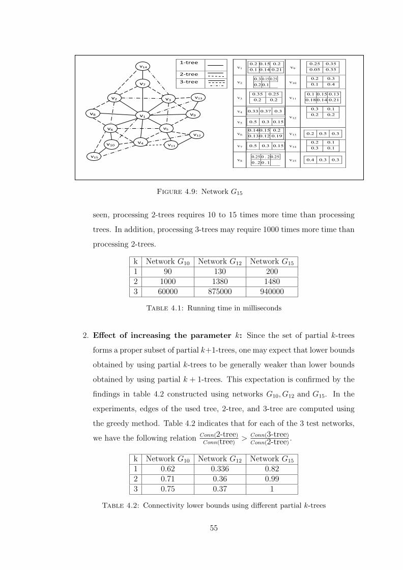
v1 0.2 0.15 0.20.1 0.14 0.21

v9 0.25 0.35 0.05 0.35

v2 0.3 0.15 0.250.2 0.1

v10 0.2 0.3 0.1 0.4

v3 0.35 0.250.2 0.2

v11 0.1 0.15 0.13 0.18 0.14 0.21

v4 0.33 0.37 0.3

v12

0.3 0.1 0.2 0.2

v5 0.5 0.3 0.15

v6 0.140.15 0.20.130.12 0.19 v13 0.2 0.5 0.3

v7 0.5 0.3 0.15

v14 0.2 0.1 0.3 0.1

v8 0.25 0 . 2 0.250 . 2 0 . 1

v15 0.4 0.3 0.3

 v1 

1‐tree   

2‐tree   

3‐tree    v7 

 v3  v2 

 v14 

 v6   v5 

 v4 

 v9 v8 

v10 

 v15 

 v11 

v12

v13

Figure 4.9: Network G15

seen, processing 2-trees requires 10 to 15 times more time than processing

trees. In addition, processing 3-trees may require 1000 times more time than

processing 2-trees.

k Network G10 Network G12 Network G15

1 90 130 2002 1000 1380 14803 60000 875000 940000

Table 4.1: Running time in milliseconds

2. Effect of increasing the parameter k: Since the set of partial k-trees

forms a proper subset of partial k+1-trees, one may expect that lower bounds

obtained by using partial k-trees to be generally weaker than lower bounds

obtained by using partial k + 1-trees. This expectation is confirmed by the

findings in table 4.2 constructed using networks G10, G12 and G15. In the

experiments, edges of the used tree, 2-tree, and 3-tree are computed using

the greedy method. Table 4.2 indicates that for each of the 3 test networks,

we have the following relation Conn(2-tree)Conn(tree) > Conn(3-tree)

Conn(2-tree) .

k Network G10 Network G12 Network G15

1 0.62 0.336 0.822 0.71 0.36 0.993 0.75 0.37 1

Table 4.2: Connectivity lower bounds using different partial k-trees

55

3. Effect of increasing node transmission range: Intuitively, increasing

node transmission range Rtr of a given probabilistic network G has two

effects:

(a) increasing the number of edges in the network and

(b) increasing the probability that any given edge arises.

Consequently, denser partial k-tree subgraphs with better edge probabilities

can be found. Thus, Conn(G) is expected to increase. Figure 4.10 explores

this aspect for network G10 when Rtr varies in the range [5.5, 9.5] and a

tree (partial 2-tree, or 3-tree) subgraph is selected randomly. As can be

seen, bounds obtained by using a tree (2-tree, or a 3-tree) increases as Rtr

increases.

0

0.1

0.2

0.3

0.4

0.5

0.6

0.7

0.8

0.9

1

5 5.5 6 6.5 7 7.5 8 8.5 9

Connecti

vit

y

Transmission Range

1-tree

2-tree

3-tree

Figure 4.10: Connectivity ver-sus transmission range with random

subgraph selection

0

0.1

0.2

0.3

0.4

0.5

0.6

0.7

0.8

0.9

1

5 5.5 6 6.5 7 7.5 8 8.5 9

Co

nn

ecti

vit

y

Transmission Range

1-tree

2-tree

3-tree

Figure 4.11: Connectivity versustransmission range with greedy sub-

graph selection

4. Effect of subgraph selection method: Intuitively, for any given k, lower

bounds obtained from partial k-tree subgraphs obtained using the greedy

method (c.f. Chapter 2) are likely to be better than lower bounds obtained

using the random method. To investigate this aspect, we compute lower

bounds on network G10 (used to generate figure 4.11) when we use partial

k-tree subgraphs computed using the greedy method. The obtained results

confirm the above intuition. For example, consider the bounds obtained

56

by using tree subgraphs when Rtr = 6. For this scenario, figure 4.10 gives

Conn(G) ≥ 0 whereas figure 4.11 gives Conn(G) ≥ 0.1

4.8 Concluding Remarks

In this chapter, we have extended the dynamic programming approach used in

Chapter 3 to handle the A-CONN problem on any probabilistic network whose

underlying graph is a partial k-tree G, assuming that a PES of G is given. The

algorithm runs in polynomial time for any fixed k. It provides a network design

tool for analyzing probabilistic connectivity when any combination of the following

parameters change: node locality sets, their probabilistic distribution, and node

transmission range.

57

Chapter 5

Networks with Relays

In this chapter, we extend the dynamic program of Chapter 4 for solv-

ing the A-CONN problem on partial k-trees to solve the AR-CONN

and SR-CONN problems. For each problem, we present the modi-

fications required, analyze the running time, and present simulation

results to explore some performance and usage aspects.

5.1 Overview of the Extensions

Throughout this chapter, the UWSN is modelled by a probabilistic graph G =

(V = Vsense ∪ Vrelay , EG, Loc, p) where V = Vsense ∪ Vrelay, and Vrelay may contain

zero or more relay nodes. As in Chapter 4, we assume that G has the topology

of a partial k-tree for some specified k. In addition, when no confusion arises,

we use G to refer also to the partial k-tree graph underlying the structure of the

probabilistic graph G.

Our proposed extended algorithm for solving the AR-CONN and SR-CONN prob-

lems have the same structure and organization as the algorithm presented in Chap-

ter 4. Functions Main and t merge (but not p merge) are modified, but maintain

their high level structure and steps. As discussed below, the main modifications

concern the formulation of new network state types to solve each problem. The

58

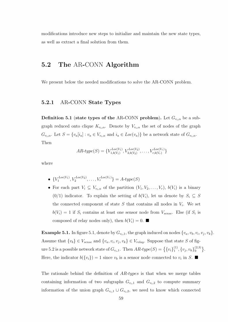
modifications introduce new steps to initialize and maintain the new state types,

as well as extract a final solution from them.

5.2 The AR-CONN Algorithm

We present below the needed modifications to solve the AR-CONN problem.

5.2.1 AR-CONN State Types

Definition 5.1 (state types of the AR-CONN problem). Let Gvi,α be a sub-

graph reduced onto clique Kvi,α. Denote by Vvi,α the set of nodes of the graph

Gvi,α. Let S = {va[ia] : va ∈ Vvi,α and ia ∈ Loc(va)} be a network state of Gvi,α.

Then

AR-type(S) = {V Loc(V1)1,b(V1)

, VLoc(V2)2,b(V2)

, . . . , VLoc(Vr)r,b(Vr)

}

where

• {V Loc(V1)1 , V

Loc(V2)2 , . . . , V

Loc(Vr)r } = A-type(S)

• For each part Vi ⊆ Vvi,α of the partition (V1, V2, . . . , Vr), b(Vi) is a binary

(0/1) indicator. To explain the setting of b(Vi), let us denote by Si ⊆ S

the connected component of state S that contains all nodes in Vi. We set

b(Vi) = 1 if Si contains at least one sensor node from Vsense. Else (if Si is

composed of relay nodes only), then b(Vi) = 0. �

Example 5.1. In figure 5.1, denote byGvi,1, the graph induced on nodes {va, vb, vi, vj, vk}.Assume that {vb} ∈ Vsense and {va, vi, vj, vk} ∈ Vrelay. Suppose that state S of fig-

ure 5.2 is a possible network state ofGvi,1. ThenAR-type(S) ={{vi}(1)1 , {vj, vk}(2,3)0

}.

Here, the indicator b({vi}) = 1 since vb is a sensor node connected to vi in S. �

The rationale behind the definition of AR-types is that when we merge tables

containing information of two subgraphs Gvi,1 and Gvi,2 to compute summary

information of the union graph Gvi,1 ∪ Gvi,2, we need to know which connected

59

 

vl

vb vi

vj

va

vk

Sensor node

Relay node

Figure 5.1: A fragment of a 3-tree

 

vi[1]

va[1]

vb[2]

vk[3]

vj[2]

Figure 5.2: A state S on{va, vb, vi, vj , vk}

components contain at least one sensor node (and thus, are essential to form an

operating state), or contain relay nodes only (and thus, may not be essential to

form an operating state).

5.2.2 Initializing Tables

Step 1 of function Main initializes a table TH associates with each k-cliques H of

the full graph k-tree(G). Similar to the approach used in Chapter 4, we perform

the following steps,

1. We construct for each edge e = {x, y} in H an exhaustive table Te where

the keys are of the AR-type.

2. We use t merge and p merge to compute the cross product of all tables

associated with all edges in the k-clique H.

5.2.3 Merging AR-CONN State Types

We recall that function t merge takes as input two table T1 and T2 that may have

a set C = V (T1) ∩ V (T2) of common nodes, and produces a new table Tout. The

context of the merge operation is as follows.

Each table Ti, i = 1, 2, contains summary information about a subgraph Gi that

has been reduced onto a clique Ki. The merge operation computes a table Tout

that stores summary information about the graph G1 ∪G2.

60

Tout is computed by processing each pair of keys (i.e., AR-CONN state types)

key1 ∈ T1 and key2 ∈ T2. Processing key1 and key2 results in a new state type,

denoted keyout, and an associated probability, denoted pout. To explain process-

ing of key1 and key2, consider two network states: Si, i = 1, 2, of the subgraph

Gi reduced onto the clique Ki, where keyi = AR-type(Si). Merging S1 and S2

generates keyout = AR-type(S1 ∪ S2).

As in Chapter 4, such a union is possible only if each common node in C assumes

the same position in both of S1 and S2. Else, the two keys are not compatible,

and no keyout is generated.

To explain the structure of keyout (if it exists), let

AR-type(S1) = {XLoc(Xi)i,b(Xi)

: i = 1, 2, . . .},AR-type(S2) = {Y Loc(Lj)

j,b(Yj): j = 1, 2, . . .}, and

AR-type(S1 ∪ S2) = {ZLoc(Zk)k,b(Zk)

: k = 1, 2, . . .}

.

Then

• The partition {Zk : k = 1, 2, } is generated by applying partition merge to

{Xi : i = 1, 2, . . .} and {Yj : j = 1, 2, . . .}.• The binary indicator obtained by merging two parts, say Xi and Yj is

max(b(Xi), b(Yj)).

Similar to the A-CONN algorithm, the probability pout is the product T1(key1)×T2(key2) divided by a correction term =

∏(px(i) : x[i] is common between key1 and key2

).

5.2.4 Removing Bad State Types

We recall that the first part of the main loop of function Main merges all tables

{Tvi,α : α = base, 1, 2, . . . , k} into table Tvi,base. The second part of the main loop

61

(Steps 7 to 10) removes bad state types from table Tvi,base prior to deleting node

vi. For the AR-CONN problem, a state S of the subgraph Gvi,base reduced onto

the k-clique Kvi,base is considered bad at this stage if node vi appears as a singleton

part in the partition associated with AR-type(S) and the indicator b(vi) = 1.

This badness follows since S has a connected component with at least one sensor

node, and this component reaches outside nodes via node vi, yet node vi is dis-

connected from other nodes in Kvi,base. The algorithm removes all such bad state

types from Tvi,base.

Else if AR-types(S) is good then one of the following cases applies:

• Case: vi is a singleton part and b({vi}) = 0. Here, the part {vi} is

merely removed from AR-type(S).

• Case: vi is not singleton. Assume that vi belong to part V1, where

|V1| ≥ 2. Then node vi and its associated position is removed from V1.

5.2.5 Obtaining Final Result

Step 11 of function Main is modified to compute Conn(G) as the sum of all values

in table Tvn−k,base corresponding to AR-types of the form

{XLoc(Xi)i,b(Xi)

: i = 1, 2, . . .}where

• the particular part of the partition X1, X2, . . . , Xr that contains the sink

node, say X1, has b(X1) = 1, and

• each other part Xj, j 6= 1, of the partition has b(Xj) = 0.

That is, step 11 considers only network states where any connected component

disconnected from the sink does not have any sensor node. Thus, all sensor nodes

must lie in the same component of the sink node.

62

5.2.6 Running Time

As in Chapter 4, n denotes the number of nodes in G, lmax denotes the maximum

number of locations in the locality set of any node, and Bk denote the kth Bell

number.

Theorem 5.2. In the AR-CONN algorithm we have

1. The maximum length of any table is O(Bklkmax2

k)

2. The worst case running time is O(n(Bklkmax2

k)2)

The proof is similar to the proof of the Theorem 4.3 by observing that adding

indicator bits to state types makes the maximum table length as specified in part

1.

5.3 AR-CONN Simulation Results

Relay nodes are expected to be cheaper than sensor nodes since they do not

include sensing devices. In addition, relay nodes are not required to do energy

consuming data acquisition tasks as sensor nodes. Hence, their design may enjoy

more flexibility than sensor nodes, and their energy supply is expected to last

longer.

In this section we utilize the algorithm developed for the AR-CONN problem to

investigate the positive effects of deploying relay nodes.

Test Networks: To illustrate our basic findings, we present results on network

G10 (figure 5.3) and network G10,3 (figure 5.4) which adds 3 relay nodes to G10.

In each network, v1 is the sink node, and all edges shown in the figures appear

when Rtr ≥ 6.5 units. Reducing Rtr results in networks with possibly fewer edges.

We experiment with a tree, 2-tree, and 3-tree subgraphs shown by the solid and

dotted lines in the figure. The subgraphs are obtained using the greedy method

of Chapter 2.

63

 

v1 0.2 0.5 0.10.150.05

v6 0.6 0.2 0.1 0.1

v2 0.25 0.3 0.16 0.29 v7 0.5 0.25 0.2

v3 0.2 0.3 0.10.1 0.15 0.15 v8

0.25 0.360.14 0.25

v4 0.25 0.350.25 0.15 v9 0.7 0.15 0.15

v5 0.16 0.18 0.140.3 0.22 v10

0.18 0.24 0.34 0.1 0.14

v8 v10 

 v1 

v7

 v9 

 v6  v5 

 v4 

 v2 

v3

1‐tree   

2‐tree   

3‐tree   

Figure 5.3: Network G10 

 

 

 

 

v1 0.2 0.5 0.1 0.150.05

v6 0.6 0.2 0.1 0.1

v2 0.25 0.3 0.16 0.29 v7 0.5 0.25 0.2

v3 0.2 0.3 0.1 0.1 0.15 0.15 v8

0.25 0.360.14 0.25

v4 0.25 0.35 0.25 0.15 v9 0.7 0.15 0.15

v5 0.16 0.18 0.14 0.3 0.22 v10

0.18 0.24 0.34 0.1 0.14

v11 0.2 0.45 0.25 v12 0.6 0.4

v13 0.5 0.5

v8 v10 

 v1 

v7

v9

v6 v5 

v4

v2

v3

 v12

 v11

 v13

1‐tree   

2‐tree   

3‐tree   

Figure 5.4: Network G10,3

1. Running Time: Table 5.1 shows the increase of running time as the dy-

namic program moves from using A-type keys on G10 to using AR-type keys

on G10,3

k Network G10 Network G10,3

1 90 1102 1000 60003 6000 8000

Table 5.1: Running time in milliseconds

64

2. Effect of adding relay nodes: Table 5.2 shows the obtained bounds onG10

and G10,3. As can be seen, adding 3 relay nodes can enhance the computed

Conn(G) by, e.g. 63% (the 3rd row).

k Network G10 Network G10,3

1 0.30 0.862 0.54 0.963 0.60 0.98

Table 5.2: Connectivity with respect to k

3. Effect of adding relay nodes for various node Rtr: Figure 5.5 illustrates

Conn(G), on G10 and G10,3 as Rtr varies in the range [2.5, 7.5]. Each obtained

curve exhibits a notable monotonic increasing behaviour as Rtr increases. As

explained in Chapter 4, this behaviour is due to the appearance of more edges

as Rtr increases, and the potential increase in the probability of each edge

as Rtr increases. Increasing Rtr, however, requires increasing node energy

consumption. To achieve a desired Conn(G) value, a designer may utilize

the obtained curves to assess the merit of increasing Rtr versus deploying

more relay nodes.

0

0.1

0.2

0.3

0.4

0.5

0.6

0.7

0.8

0.9

1

2.5 3 3.5 4 4.5 5 5.5 6 6.5 7 7.5

Conn

ectiv

ity

Transmission Range

1-Tree-w-R

2-Tree-w-R

3-Tree-w-R

1-Tree

2-Tree

3-Tree

Figure 5.5: Connectivity versus transmission range

65

5.4 The SR-CONN Algorithm

Next, we present the needed modifications to solve the SR-CONN problem.

5.4.1 SR-CONN State Types

Definition 5.3 (state types of the SR-CONN problem). Let Gvi,α be a sub-

graph reduced onto a clique Kvi,α. Denote by Vvi,α the set of nodes of the graph

Gvi,α. Let S = {va[ia] : va ∈ Vvi,α and ia ∈ Loc(va)} be a network state of Gvi,α.

Then

SR-type(S) = {V Loc(V1)1,c(V1)

, VLoc(V2)2,c(V2

, . . . , VLoc(Vr)r,c(Vr

}

where

• {V Loc(V1)1 , V

Loc(V2)2 , . . . , V

Loc(Vr)r } = A-type(S)

• For each part Vi ⊆ Vvi,α of partition (V1, V2, . . . , Vr), c(Vi) is the number of

sensor nodes in the connected component Si ⊆ S that includes all nodes in

Vi. �

Example 5.2. In figure 5.6, denote byGvi,1, the graph induced on nodes {va, vb, vi, vj, vk}.Assume that {vb, vi} ∈ Vsense and {va, vj, vk} ∈ Vrelay. Suppose that state S of fig-

ure 5.7 is a possible network state ofGvi,1. Then SR-type(S) ={{vi}(1)2 , {vj, vk}(2,3)0

}.

Here, the count c({vi}) = 2 since both of vi and vb are sensor nodes. �

 

vl

vb

vj

va

vk

Sensor node

Relay node

vi

Figure 5.6: A 3-tree fragment

 

va[1]vb[2]

vk[3]

vj[2]

vi[1]

Figure 5.7: A state S on{va, vb, vi, vj , vk}

66

The rationale behind the definition of the SR-type is that when we merge tables

containing summary information of two subgraphs G1 and G2 to compute sum-

mary information of the union graph G1 ∪G2, we need to know how many sensor

nodes are in each connected component of each state S summarized in the class

SR-type(S).

5.4.2 Initializing Tables

Step 1 of function Main initializes a table TH associates with each k-cliques H of

the full graph k-tree(G). Our approach here is similar to the one used in Section

5.2.2

5.4.3 Merging SR-CONN State Types

Using the same notation of section 5.2.3, we explain how to process a pair of keys:

key1 ∈ T1 and key2 ∈ T2, where T1 and T2 are two tables to be merged.

We consider two network states: Si, i = 1, 2, where Si is a network state of the

subgraph Gi reduced onto the clique Ki, where keyi = SR-type(Si). Merging S1

and S2 generates keyout = SR-type(S1 ∪ S2).

As with keys of the A-type (or AR-type) the union S1 ∪ S2 is possible only if each

common node between S1 and S2 takes the same position in both states.

Now, let

SR-type(S1) = {XLoc(Xi)i,c(Xi)

: i = 1, 2, . . .},SR-type(S2) = {Y Loc(Lj)

j,c(Yj): j = 1, 2, . . .}, and

SR-type(S1 ∪ S2) = {ZLoc(Zk)k,c(Zk)

: k = 1, 2, . . .}

Then

• The partition {Zk : k = 1, 2, } is generated by applying partition merge to

{Xi : i = 1, 2, . . .} and {Yj : j = 1, 2, . . .}.67

• If parts Xi and Yj are merged together into Zk, and the number of common

sensor nodes between Xi and Yj is denoted nij then

c(Zk) = max(nreq, c(Xi) + c(Yj)− nij).

Similar to the A-CONN algorithm, the probability pout is the product T1(key1)×T2(key2) divided by a correction term =

∏(px(i) : x[i] is common between key1 and key2).

5.4.4 Bad State Types

Using the same context and notation of section 5.2.4, we define in this section bad

SR-CONN state types. For a given node vi that is processed in some iteration of

the main loop of function Main, the first part of function Main merges all tables

{Tvi,α : α = 1, 2, . . . , k, base} into table Tvi,base.

For a state S of Gvi,base, let nsense(S) be the number of sensor nodes that can

reach the rest of the graph by nodes in the separator clique Kvi,base. Thus, if

SR-type(S) = {XLoc(Xi)i,c(Xi)

: i = 1, 2, . . . , r} then

nsense(S) =

∑

Xj 6={vi}c(Xj) if node vi appears as a singleton in the partition

(X1, X2, . . . , Xr)∑

j=1,2,...,r

c(Xj) otherwise

Now, let us denote by nvi,base,sense the number of sensor nodes in the subgraph

Gvi,base reduced onto the k-clique Kvi,base at the end of the first part of the main

loop in function Main. Thus, |Vsense| − nv,base,sense is the number of sensor nodes

outside the graph Gvi,base. By definition of operating states of the SR-CONN

problem, SR-type(S) is bad if

nsense(S) + (|Vsense| − nvi,base,sense) ≤ nreq.

68

We recall that the algorithm removes all such bad state types from Tvi,base in step

9 of function Main. Else, if SR-type(S) is good then the algorithm just removes

node vi and its associated position from SR-type(S).

5.4.5 Obtaining Final Result

Step 11 of function Main computes Conn(G, nreq) as the sum of all values in the

table Tvn−k,base corresponding to keys of the form

{XLoc(Xi)i,c(Xi)

: i = 1, 2, . . .}

where the partition part that contains the sink node, say X1, has c(X1) ≥ nreq.

5.4.6 Running Time

As in Chapter 4, n denotes the number of nodes in G, lmax denotes the maximum

number of locations in the locality set of any node, and Bk denote the kth Bell

number.

Theorem 5.4. In the SR-CONN algorithm we have

1. The maximum length of any table is O(Bklkmaxn

kreq)

2. The worst case running time is O(n(Bklkmaxn

kreq)

2)

The proof is similar to the proof of the Theorem 4.3 by observing that adding the

counters c(Vi) to state types makes the maximum table length as specified in part

1.

5.5 SR-CONN Simulation Results

The SR-CONN problem is motivated by applications where an UWSN task can

be achieved by any subset of sensor nodes connected the sink and has size ≥ nreq

69

nodes, where nreq is a design parameter. For such applications, a designer has at

least 3 options to achieve a minimum required Conn(G, nreq) value:

• tuning the nreq parameter,

• tuning node transmission range Rtr, and

• tuning the number of deployed relay nodes.

In this section we explore the use of our devised SR-CONN algorithm to tackle

such design problem.

Test Networks: As in section 5.3, we use network G10 in figure 5.3 and G10,3 in

figure 5.4

Effect of varying nreq: Figure 5.8 illustrates the achieved Conn(G, nreq) as nreq

varies in the range [1, 10]. Figure 5.9 illustrates the achieved Conn(G, nreq) as nreq

varies in the range [1, 10], and Rtr varies in the range [2.5, 5.5].

Connecti

vit

y

nreq

1-Tree

2-Tree

3-Tree

Figure 5.8: Connectivity versusnreq

Figure 5.9: Connectivity versusnreq and transmission range

5.6 Concluding Remarks

In this chapter we have presented extensions to the A-CONN dynamic program-

ming algorithm. The extensions yield two algorithms for solving the AR-CONN

70

and SR-CONN problem on partial k-trees where a k-PES is specified for each

problem instance. The algorithms run in polynomial time on any partial k-tree

with fixed k. The algorithms are implemented in C++ and provide network de-

sign tools for analyzing probabilistic connectivity when any combination of the

following parameters change: node locality sets and their probabilistic distribu-

tion, node transmission range, number of relay nodes that can be deployed, and

the number of nodes connected to the sink required achieve a given task.

71

Chapter 6

Concluding Remarks

The work in this thesis has been motivated by recent interest in UWSNs as a

platform for preforming many useful tasks. A challenge arises since sensor nodes

incur small scale and large scale movements that can disrupt network connectivity.

Thus, tools for quantifying the likelihood that a network remains completely or

partially connected become of interest.

To this end, the thesis has formalized 4 probabilistic connectivity problems, de-

noted A-CONN, S-CONN,AR-CONN, and SR-CONN. The obtained results show

that all of the 4 problems admit polynomial time algorithms on k-trees (and their

subgraphs), for any fixed k. The running times of the algorithms, however, in-

crease exponentially as k increases. Thus, more work needs to be done towards

obtaining more effective algorithms.

For future research, we propose the following directions.

• As mentioned in Chapter 1, the class of probabilistic connectivity problems

discussed in the thesis shares some similarity with the class of network relia-

bility problems discussed in [23, 51]. Both classes of problems utilize a type

of probabilistic graphs to formalize the problems, and core problems in each

class are #P -hard problems.

In [23], a number of methods are devised to cope with the problems. These

methods aim at finding classes of graphs for which the problems can be

72

solved effectively, as well as deriving lower and upper bounds from disjoint or

overlapping subgraphs that form either pathsets or cutsets. Investigating the

applicability of such methods to probabilistic connectivity problems appears

to be a worthwhile direction.

• Some wireless sensor network applications require that sensor nodes repeat-

edly perform data collection rounds. In each round, sensor nodes collect

data and forward the collected data to the sink node using multihop routes.

Existing results in the literature (e.g., [46]) have shown that the direction

of water currents influence delays in underwater acoustic communication.

Given randomness in the position of UWSN nodes, it becomes interesting to

analyze the delays incurred in typical data collection rounds.

• Area coverage analysis is a topic that has received attention in UWSNs. In

light of node mobility in UWSNs, it appears worthwhile to investigate area

coverage assuming a probabilistic locality model of the nodes.

73

Bibliography

[1] K. Akkaya and A. Newell. Self-deployment of sensors for maximized cov-

erage in underwater acoustic sensor networks. Computer Communications,

32(7):1233–1244, 2009.

[2] I. F. Akyildiz, D. Pompili, and T. Melodia. Underwater acoustic sensor net-

works: research challenges. Ad hoc networks, 3(3):257–279, 2005.

[3] S. M. N. Alam and Z. J. Haas. Coverage and Connectivity in Three-

Dimensional Underwater Sensor Networks. Wireless Communication and Mo-

bile Computing (WCMC), 8(8):995–1009, 2008.

[4] H. M. Ammari and S. K. Das. A Study of k -coverage and measures of con-

nectivity in 3D wireless sensor networks. IEEE Transactions on Computers,

59(2):243–257, 2010.

[5] S. Arnborg, D. G. Corneil, and A. Proskurowski. Complexity of finding em-

beddings in a k -tree. SIAM Journal on Algebraic Discrete Methods, 8(2):277–

284, 1987.

[6] S. Arnborg, J. Lagergren, and D. Seese. Easy problems for tree-decomposable

graphs. Journal of Algorithms, 12(2):308–340, 1991.

[7] S. Arnborg and A. Proskurowski. Linear time algorithms for NP-hard prob-

lems restricted to partial k -trees. Discrete Applied Mathematics, 23(1):11–24,

1989.

74

[8] M. Ayaz, I. Baig, A. Abdullah, and I. Faye. A survey on routing techniques

in underwater wireless sensor networks. Journal of Network and Computer

Applications, 34(6):1908–1927, 2011.

[9] Y. Bayrakdar, N. Meratnia, and A. Kantarci. A comparative view of routing

protocols for underwater wireless sensor networks. In OCEANS, 2011 IEEE-

Spain, pages 1–5. IEEE, 2011.

[10] L. W. Beineke and R. E. Pippert. The enumeration of labelled 2-trees. Notices

American Mathematical Society, 15:384, 1968.

[11] L. W. Beineke and R. E. Pippert. The number of labelled k -dimensional trees.

Journal of Combinatorial Theory, 6(2):200–205, 1969.

[12] H. L. Bodlaender. Dynamic programming on graphs with bounded treewidth.

In Proceeding 15th International Colloquium on Automata, Languages and

Programming, volume 317 of Lecture Notes in Computer Science, pages 105–

118. Springer Berlin Heidelberg, 1988.

[13] H. L. Bodlaender. A linear time algorithm for finding tree-decompositions of

small treewidth. In Proceedings of the twenty-fifth annual ACM symposium

on Theory of computing, pages 226–234. ACM, 1993.

[14] A. S. Bower. A simple kinematic mechanism for mixing fluid parcels across a

meandering jet. Journal of Physical Oceanography, 21(1):173–180, 1991.

[15] A. S. Bower and T. Rossby. Evidence of cross-frontal exchange processes

in the gulf stream based on isopycnal rafos float data. Journal of Physical

Oceanography, 19(9):1177–1190, 1989.

[16] A. Brandstadt, V. Bang Le, and J. P. Spinrad. Graph classes: a survey,

volume 3. SIAM, Philadelphia, PA, USA, 1999.

[17] R. A. Brualdi. Introductory combinatorics 5th Edition. Pearson, New York,

2009.

75

[18] A. Caruso, F. Paparella, L. F. M. Vieira, M. Erol, and M. Gerla. The me-

andering current mobility model and its impact on underwater mobile sensor

networks. In The 27th Conference on Computer Communications IEEE IN-

FOCOM, pages 221–225. IEEE, 2008.

[19] Y. Cengel and J. Cimbala. Fluid Mechanics Fundamentals and Applications.

McGraw-Hill Education, 2013.

[20] V. Chandrasekhar, W. K. Seah, Y. S. Choo, and H. V. Ee. Localization in

underwater sensor networks: survey and challenges. In Proceedings of the 1st

ACM international workshop on Underwater networks, pages 33–40. ACM,

2006.

[21] K. Chen, M. Ma, E. Cheng, F. Yuan, and W. Su. A Survey on MAC protocols

for underwater wireless sensor networks. Number 99, pages 1–15. 2014.

[22] S. Climent, A. Sanchez, J. V. Capella, N. Meratnia, and J. J. Serrano. Un-

derwater Acoustic Wireless Sensor Networks: Advances and Future Trends

in Physical, MAC and Routing Layers. Sensors, 14(1):795–833, 2014.

[23] C. J. Colbourn. The Combinatorics of Network Reliability. Oxford University

Press, Inc., New York, USA, 1987.

[24] T. H. Cormen, C. E. Leiserson, R. L. Rivest, C. Stein, et al. Introduction to

algorithms. 3rd Edition, MIT press, Cambridge, 2009.

[25] E. S. Elmallah and C. J. Colbourn. The complexity of some edge deletion

problems. IEEE Transactions on Circuits and Systems, 35(3):354–362, 1988.

[26] M. Erol, S. Oktug, L. Vieira, and M. Gerla. Performance evaluation of dis-

tributed localization techniques for mobile underwater acoustic sensor net-

works. Ad Hoc Networks, 9(1):61–72, 2011.

[27] M. Erol, F. Vieira, A. Caruso, F. Paparella, M. Gerla, and S. Oktug. Multi

stage underwater sensor localization using mobile beacons. In Second Inter-

national Conference on Sensor Technologies and Applications, 2008. SEN-

SORCOMM’08., pages 710–714. IEEE, 2008.

76

[28] M. Erol, L. F. M. Vieira, and M. Gerla. Localization with dive’n’rise (dnr)

beacons for underwater acoustic sensor networks. In Proceedings of the Second

Workshop on Underwater Networks, WuWNet ’07, pages 97–100, New York,

NY, USA, 2007. ACM.

[29] Alan C. F. and Jun P. Performance of IEEE 802.11 MAC in underwater

wireless channels. Procedia Computer Science, 10(0):62 – 69, 2012.

[30] N. Fair, A. Chave, L. Freitag, J. Preisig, S. White, D. Yoerger, and F. Son-

nichsen. Optical modem technology for seafloor observatories. In OCEANS

2006, pages 1–6. IEEE, 2006.

[31] L Freitag, M Grund, J Catipovic, D Nagle, B Pazol, and J Glynn. Acoustic

communication with small uuvs using a hull-mounted conformal array. In

MTS/IEEE Conference and Exhibition OCEANS, 2001., volume 4, pages

2270–2275. IEEE, 2001.

[32] A. Ghosh and S. K. Das. Coverage and connectivity issues in wireless sensor

networks: A survey. Pervasive and Mobile Computing, 4(3):303–334, 2008.

[33] C. Giantsis and A. A. Economides. Comparison of routing protocols for un-

derwater sensor networks: a survey. International Journal of Communication

Networks and Distributed Systems, 7(3):192–228, 2011.

[34] A. Gkikopouli, G. Nikolakopoulos, and S. Manesis. A survey on underwater

wireless sensor networks and applications. In 20th Mediterranean Conference

on Control & Automation (MED) 2012, pages 1147–1154. IEEE, 2012.

[35] M. C. Golumbic. Algorithmic graph theory and perfect graphs, volume 57.

North-Holland Publishing Co., Amsterdam, Netherland, 2004.

[36] J. Heidemann, M. Stojanovic, and M. Zorzi. Underwater sensor networks:

applications, advances and challenges. Philosophical Transactions of the Royal

Society A: Mathematical, Physical and Engineering Sciences, 370(1958):158–

175, 2012.

77

[37] M. T. Isik and O. B. Akan. A three dimensional localization algorithm for

underwater acoustic sensor networks. IEEE Transactions on Wireless Com-

munications, 8(9):4457–4463, 2009.

[38] M. A. Islam and E. S. Elmallah. Tree Bound on Probabilistic Connectivity

of Underwater Sensor Networks. In The 13th IEEE WLN workshop 2014 (To

appear).

[39] U. Lee, P. Wang, Y. Noh, F. Vieira, M. Gerla, and J. Cui. Pressure routing

for underwater sensor networks. In 2010 Proceedings IEEE INFOCOM, pages

1–9. IEEE, 2010.

[40] Y. Noh, U. Lee, P. Wang, B. S. C. Choi, and M. Gerla. Vapr: Void-aware

pressure routing for underwater sensor networks. Mobile Computing, IEEE

Transactions on, 12(5):895–908, 2013.

[41] J. Partan, J. Kurose, and B. N. Levine. A survey of practical issues in under-

water networks. ACM SIGMOBILE Mobile Computing and Communications

Review, 11(4):23–33, 2007.

[42] C. Petrioli, R. Petroccia, and M. Stojanovic. A comparative performance

evaluation of MAC protocols for underwater sensor networks. In OCEANS

2008, pages 1–10. IEEE, 2008.

[43] D. Pompili, T. Melodia, and I. F. Akyildiz. Deployment analysis in un-

derwater acoustic wireless sensor networks. In Proceedings of the 1st ACM

international workshop on Underwater networks, pages 48–55. ACM, 2006.

[44] D. Pompili, T. Melodia, and I. F. Akyildiz. Routing algorithms for delay-

insensitive and delay-sensitive applications in underwater sensor networks. In

Proceedings of the 12th annual international conference on Mobile computing

and networking, pages 298–309. ACM, 2006.

[45] A. Proskurowski. Separating subgraphs in k -trees: Cables and caterpillars.

Discrete Mathematics, 49(3):275–285, 1984.

78

[46] L. Pu, Y. Luo, H. Mo, Z. Peng, J. Cui, and Z. Jiang. Comparing underwater

MAC protocols in real sea experiment. In IFIP Networking Conference, 2013,

pages 1–9. IEEE, 2013.

[47] Y. Ren, W. K. Seah, and P.l D. Teal. Performance of pressure routing in

drifting 3D underwater sensor networks for deep water monitoring. In Pro-

ceedings of the seventh ACM international conference on underwater networks

and systems, page 28. ACM, 2012.

[48] A. Reza and J. Harms. Robust grid-based deployment schemes for under-

water optical sensor networks. In IEEE 34th Conference on Local Computer

Networks, 2009. LCN 2009., pages 641–648. IEEE, 2009.

[49] N. Robertson and P. D. Seymour. Graph minors. II. Algorithmic aspects of

tree-width. Journal of Algorithms, 7(3):309–322, 1986.

[50] F. Senel, K. Akkaya, and T. Yilmaz. Autonomous deployment of sensors

for maximized coverage and guaranteed connectivity in Underwater Acoustic

Sensor Networks. In 2013 IEEE 38th Conference on Local Computer Networks

(LCN), pages 211–218. IEEE, 2013.

[51] D. R. Shier. Network reliability and algebraic structures. Clarendon Press,

New York, USA, 1991.

[52] H. Tan, R. Diamant, W. K. Seah, and M. Waldmeyer. A survey of techniques

and challenges in underwater localization. Ocean Engineering, 38(14):1663–

1676, 2011.

[53] A. Y. Teymorian, W. Cheng, L. Ma, X. Cheng, X. Lu, and Z. Lu. 3D under-

water sensor network localization. IEEE Transactions on Mobile Computing,

8(12):1610–1621, 2009.

[54] J. A. Wald and C. J. Colbourn. Steiner trees in probabilistic networks. Mi-

croelectronics Reliability, 23(5):837–840, 1983.

79

[55] M. A. Yigitel, O. D. Incel, and C. Ersoy. QoS-aware MAC protocols for

wireless sensor networks: A survey. Computer Networks, 55(8):1982–2004,

2011.

[56] L. Ying, S. Shakkottai, A. Reddy, and S. Liu. On combining shortest-path and

back-pressure routing over multihop wireless networks. IEEE/ACM Transac-

tions on Networking (TON), 19(3):841–854, 2011.

[57] F. Yunus, S. H. Ariffin, and Y. Zahedi. A survey of existing medium access

control (MAC) for underwater wireless sensor network (UWSN). In 2010

Fourth Asia International Conference on Mathematical/Analytical Modelling

and Computer Simulation (AMS), pages 544–549. IEEE, 2010.

[58] Z. Zhou, J. Cui, and S. Zhou. Efficient localization for large-scale underwater

sensor networks. Ad Hoc Networks, 8(3):267–279, 2010.

[59] Z. Zhou, Z. Peng, J. Cui, Z. Shi, and A. C. Bagtzoglou. Scalable localization

with mobility prediction for underwater sensor networks. IEEE Transactions

on Mobile Computing, 10(3):335–348, 2011.

[60] C. Zhu, C. Zheng, L. Shu, and G. Han. A survey on coverage and connec-

tivity issues in wireless sensor networks. Journal of Network and Computer

Applications, 35(2):619–632, 2012.

80