probabilistic dynamic cable rating algorithms
TRANSCRIPT

UNIVERSITY OF SOUTHAMPTON
Probabilistic Dynamic Cable Rating
Algorithms
by
Maria Angelica Hernandez Colin
A thesis submitted in fulfillment for the
degree of Doctor of Philosophy
in the
Faculty of Engineering and Physical Sciences
Electronics and Computer Science
January 2020


UNIVERSITY OF SOUTHAMPTON
ABSTRACT
FACULTY OF ENGINEERING AND PHYSICAL SCIENCES
SCHOOL OF ELECTRONICS AND COMPUTER SCIENCE
Doctor of Philosophy
by Maria Angelica Hernandez Colin
Offshore wind farm (WF) power cables are often sized using static rating calculations
as is traditionally done with cables on land. However, in practice wind farm export
cables face intermittent generation product of wind speed variations which along with
the relatively long thermal transients in the cable generate low cable temperatures. As
a consequence, offshore cables rating capabilities are often under-utilized.
Wind farm over-planting (WFO) has became a common practice to optimise offshore
cable utilisation by increasing the installed generation capacity over the static rating
limits. However, in order to avoid unnecessary power curtailment, it is necessary to
have knowledge of the actual and likely future temperatures that the cable could attain.
The use of real-time thermal rating (RTTR) methodologies is seen in the literature as
an alternative to static rating calculations in conventional installations. Nonetheless,
the use of RTTR is not enough to optimise curtailment decisions in offshore WFs as
information of future load current scenarios and conductor temperatures is needed hours
in advance.
The present research was focused on the development of probabilistic algorithms for the
hours ahead estimation of future load currents, cable temperatures and estimation of
likely risk of cable overheating. The proposed algorithms are based on a limited amount
of historical offshore data which is statistically analysed to extract seasonal behaviour
and patterns to perform the estimations. The proposed algorithms can be used as a tool
for decision making that could help the system operators to avoid power curtailment
when WFO is applied.
Further more the algorithms developed could be used as a computational tool to optimise
sizing in offshore power cables for projects in which it is necessary to reduce the levelised
cost of energy (LCOE). The application of the methodology can contribute to increase
the power delivery and decreases the cable contribution price to the LCOE.


Declaration of Authorship
I, Maria Angelica Hernandez Colin, declare that this thesis and the work presented
in it are my own and has been generated by me as the result of my own original research.
Probabilistic Dynamic Cable Rating Algorithms
I confirm that:
1. This work was done wholly or mainly while in candidature for a research degree at
this University;
2. Where any part of this thesis has previously been submitted for a degree or any other
qualification at this University or any other institution, this has been clearly stated;
3. Where I have consulted the published work of others, this is always clearly attributed;
4. Where I have quoted from the work of others, the source is always given. With the
exception of such quotations, this thesis is entirely my own work;
5. I have acknowledged all main sources of help;
6. Where the thesis is based on work done by myself jointly with others, I have made
clear exactly what was done by others and what I have contributed myself;
7. Either none of this work has been published before submission, or parts of this work
have been published as:
Hernandez-Colin M.A., Pilgrim J.A., “Offshore Cable Optimisation by Probabilistic
Thermal Risk Estimation”, International Conference on Probabilistic Methods Applied
to Power Systems (PMAPS 2018), Idaho,United States, June 2018, pp.1-6. URL.
Hernandez-Colin M.A., Pilgrim J.A.,“On-line Markov Chain Based Thermal Risk Esti-
mation for Offshore Wind Farm Cables”, 17th International Workshop on Large Scale
Integration of Wind Power into Power Systems as well as on Transmission Networks for
Offshore Wind Farms, Stockholm, Sweden, October 2018, pp.1-6. URL.
v

vi
Hernandez-Colin M.A., Pilgrim J.A.,“Assessment of financial benefits in over-planted
wind-farm export cable”, 10th International Conference on Insulated Power Cables (Ji-
cable’19), Paris Versailles France, June 2019, pp.1-6. URL.
Hernandez-Colin M.A., Pilgrim J.A.,“Cable Thermal Risk Estimation for Over-planted
Wind Farms”, IEEE Transactions on Power Delivery, Accepted May 2019, In press,
pp.1-9. URL.
Signed: . . . . . . . . . . . . . . . . . . . . . . . . . . . . . . . . . . . . . . . . . . . . . . . . . . . . . . . . . . . . . . . . . . . . . . . . . . . . . . . . . . . .
Date: . . . . . . . . . . . . . . . . . . . . . . . . . . . . . . . . . . . . . . . . . . . . . . . . . . . . . . . . . . . . . . . . . . . . . . . . . . . . . . . . . . . .
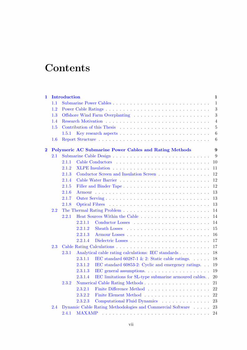
Contents
1 Introduction 1
1.1 Submarine Power Cables . . . . . . . . . . . . . . . . . . . . . . . . . . . . 1
1.2 Power Cable Ratings . . . . . . . . . . . . . . . . . . . . . . . . . . . . . . 3
1.3 Offshore Wind Farm Overplanting . . . . . . . . . . . . . . . . . . . . . . 3
1.4 Research Motivation . . . . . . . . . . . . . . . . . . . . . . . . . . . . . . 4
1.5 Contribution of this Thesis . . . . . . . . . . . . . . . . . . . . . . . . . . 5
1.5.1 Key research aspects . . . . . . . . . . . . . . . . . . . . . . . . . . 6
1.6 Report Structure . . . . . . . . . . . . . . . . . . . . . . . . . . . . . . . . 6
2 Polymeric AC Submarine Power Cables and Rating Methods 9
2.1 Submarine Cable Design . . . . . . . . . . . . . . . . . . . . . . . . . . . . 9
2.1.1 Cable Conductors . . . . . . . . . . . . . . . . . . . . . . . . . . . 10
2.1.2 XLPE Insulation . . . . . . . . . . . . . . . . . . . . . . . . . . . . 11
2.1.3 Conductor Screen and Insulation Screen . . . . . . . . . . . . . . . 12
2.1.4 Cable Water Barrier . . . . . . . . . . . . . . . . . . . . . . . . . . 12
2.1.5 Filler and Binder Tape . . . . . . . . . . . . . . . . . . . . . . . . . 12
2.1.6 Armour . . . . . . . . . . . . . . . . . . . . . . . . . . . . . . . . . 13
2.1.7 Outer Serving . . . . . . . . . . . . . . . . . . . . . . . . . . . . . . 13
2.1.8 Optical Fibres . . . . . . . . . . . . . . . . . . . . . . . . . . . . . 13
2.2 The Thermal Rating Problem . . . . . . . . . . . . . . . . . . . . . . . . . 14
2.2.1 Heat Sources Within the Cable . . . . . . . . . . . . . . . . . . . . 14
2.2.1.1 Conductor Losses . . . . . . . . . . . . . . . . . . . . . . 14
2.2.1.2 Sheath Losses . . . . . . . . . . . . . . . . . . . . . . . . 15
2.2.1.3 Armour Losses . . . . . . . . . . . . . . . . . . . . . . . . 16
2.2.1.4 Dielectric Losses . . . . . . . . . . . . . . . . . . . . . . . 17
2.3 Cable Rating Calculations . . . . . . . . . . . . . . . . . . . . . . . . . . . 17
2.3.1 Analytical cable rating calculations: IEC standards . . . . . . . . . 18
2.3.1.1 IEC standard 60287-1 & 2: Static cable ratings. . . . . . 18
2.3.1.2 IEC standard 60853-2: Cyclic and emergency ratings. . . 19
2.3.1.3 IEC general assumptions. . . . . . . . . . . . . . . . . . . 19
2.3.1.4 IEC limitations for SL-type submarine armoured cables. . 20
2.3.2 Numerical Cable Rating Methods . . . . . . . . . . . . . . . . . . . 21
2.3.2.1 Finite Difference Method . . . . . . . . . . . . . . . . . . 22
2.3.2.2 Finite Element Method . . . . . . . . . . . . . . . . . . . 22
2.3.2.3 Computational Fluid Dynamics . . . . . . . . . . . . . . 23
2.4 Dynamic Cable Rating Methodologies and Commercial Software . . . . . 23
2.4.1 MAXAMP . . . . . . . . . . . . . . . . . . . . . . . . . . . . . . . 24
vii

viii
2.4.2 CYMCAP . . . . . . . . . . . . . . . . . . . . . . . . . . . . . . . . 24
2.4.3 EPRI Dynamic Rating System DTCR . . . . . . . . . . . . . . . . 25
2.4.4 Dynamic Cable Rating Systems DCRS . . . . . . . . . . . . . . . . 25
2.4.5 Alternative Dynamic Rating Methodologies . . . . . . . . . . . . . 26
2.4.6 Application of the Existing Algorithms for Offshore WF CableRating. . . . . . . . . . . . . . . . . . . . . . . . . . . . . . . . . . 27
2.5 Cable Rating Estimation and Forecasting Methods . . . . . . . . . . . . . 28
2.5.1 Monte Carlo Simulation (MCS) . . . . . . . . . . . . . . . . . . . . 29
2.5.2 Bayesian Theory . . . . . . . . . . . . . . . . . . . . . . . . . . . . 32
2.5.3 Markov Theory . . . . . . . . . . . . . . . . . . . . . . . . . . . . . 33
2.5.4 Wind Power Generation Forecasting . . . . . . . . . . . . . . . . . 35
2.5.5 Wind Power Ramp Forecasting . . . . . . . . . . . . . . . . . . . . 36
2.5.6 Cyclic Rating Methods and Studies in Submarine Cables . . . . . 37
2.5.7 Wind Farm Overplanting and Project Optimisation . . . . . . . . 38
2.6 Summary . . . . . . . . . . . . . . . . . . . . . . . . . . . . . . . . . . . . 39
3 Probabilistic Thermal Risk Estimation Methodology 41
3.1 Offshore Wind Speed Data Analysis . . . . . . . . . . . . . . . . . . . . . 42
3.2 Load Current Time-series Profile . . . . . . . . . . . . . . . . . . . . . . . 43
3.2.1 Monthly Load Current Probability Distribution . . . . . . . . . . . 44
3.3 Notional Offshore Wind Farm . . . . . . . . . . . . . . . . . . . . . . . . . 46
3.3.1 Cable System Design Example 1 . . . . . . . . . . . . . . . . . . . 46
3.3.2 Base Case Wind Farm . . . . . . . . . . . . . . . . . . . . . . . . . 48
3.3.3 Hypothetical Overplanting Scenarios . . . . . . . . . . . . . . . . . 49
3.3.4 Example Wind Farm Assumptions . . . . . . . . . . . . . . . . . . 49
3.3.4.1 Wake Effect Losses . . . . . . . . . . . . . . . . . . . . . 50
3.3.4.2 Wind Turbine Availability . . . . . . . . . . . . . . . . . 50
3.3.4.3 Electrical Transmission Losses . . . . . . . . . . . . . . . 50
3.4 Cable Finite Difference Model . . . . . . . . . . . . . . . . . . . . . . . . . 51
3.5 Proposed Thermal Risk Estimation Methodology . . . . . . . . . . . . . . 53
3.5.1 Training and Testing Datasets . . . . . . . . . . . . . . . . . . . . 53
3.5.2 Probabilistic Load Current Generation . . . . . . . . . . . . . . . . 54
3.5.3 Probabilistic Conductor Temperature Calculation . . . . . . . . . . 55
3.5.4 Probabilistic Thermal Risk Estimation . . . . . . . . . . . . . . . . 55
3.5.5 Methodology Evaluation Process . . . . . . . . . . . . . . . . . . . 56
3.5.5.1 Accuracy of the Thermal Risk Estimations . . . . . . . . 56
3.5.5.2 Accuracy of the Methodology to Estimate Risk Ahead . . 57
3.6 Methodology Testing Results . . . . . . . . . . . . . . . . . . . . . . . . . 57
3.6.1 Accuracy of the Methodology to Estimate Thermal Risk . . . . . . 58
3.6.2 Estimated Risk Error . . . . . . . . . . . . . . . . . . . . . . . . . 60
3.6.3 Severity Analysis of Misclassifications Incidents . . . . . . . . . . . 60
3.6.4 Conductor Temperature and Risk Estimation . . . . . . . . . . . . 62
3.7 Summary . . . . . . . . . . . . . . . . . . . . . . . . . . . . . . . . . . . . 64
4 Markov Based Thermal Risk Estimation for Offshore Export Cables 67
4.1 First and Third Order Markov Models . . . . . . . . . . . . . . . . . . . . 68
4.2 Markov Based Thermal Risk Estimation Methodology . . . . . . . . . . . 68
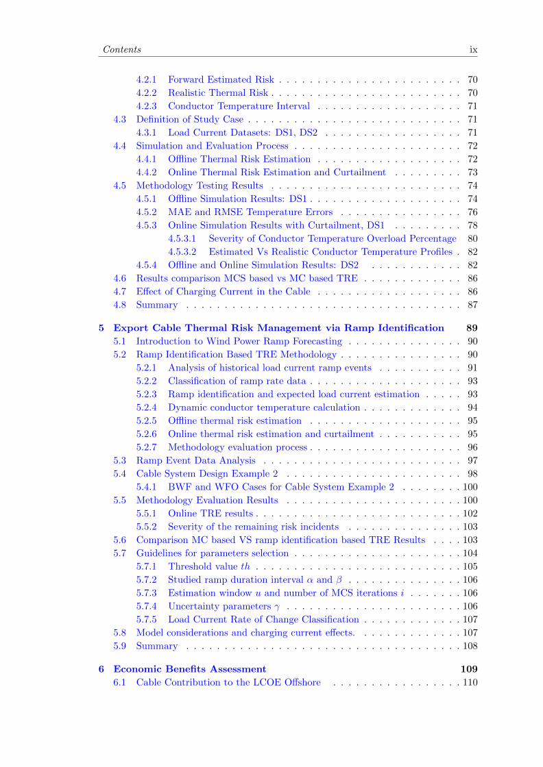
Contents ix
4.2.1 Forward Estimated Risk . . . . . . . . . . . . . . . . . . . . . . . . 70
4.2.2 Realistic Thermal Risk . . . . . . . . . . . . . . . . . . . . . . . . . 70
4.2.3 Conductor Temperature Interval . . . . . . . . . . . . . . . . . . . 71
4.3 Definition of Study Case . . . . . . . . . . . . . . . . . . . . . . . . . . . . 71
4.3.1 Load Current Datasets: DS1, DS2 . . . . . . . . . . . . . . . . . . 71
4.4 Simulation and Evaluation Process . . . . . . . . . . . . . . . . . . . . . . 72
4.4.1 Offline Thermal Risk Estimation . . . . . . . . . . . . . . . . . . . 72
4.4.2 Online Thermal Risk Estimation and Curtailment . . . . . . . . . 73
4.5 Methodology Testing Results . . . . . . . . . . . . . . . . . . . . . . . . . 74
4.5.1 Offline Simulation Results: DS1 . . . . . . . . . . . . . . . . . . . . 74
4.5.2 MAE and RMSE Temperature Errors . . . . . . . . . . . . . . . . 76
4.5.3 Online Simulation Results with Curtailment, DS1 . . . . . . . . . 78
4.5.3.1 Severity of Conductor Temperature Overload Percentage 80
4.5.3.2 Estimated Vs Realistic Conductor Temperature Profiles . 82
4.5.4 Offline and Online Simulation Results: DS2 . . . . . . . . . . . . 82
4.6 Results comparison MCS based vs MC based TRE . . . . . . . . . . . . . 86
4.7 Effect of Charging Current in the Cable . . . . . . . . . . . . . . . . . . . 86
4.8 Summary . . . . . . . . . . . . . . . . . . . . . . . . . . . . . . . . . . . . 87
5 Export Cable Thermal Risk Management via Ramp Identification 89
5.1 Introduction to Wind Power Ramp Forecasting . . . . . . . . . . . . . . . 90
5.2 Ramp Identification Based TRE Methodology . . . . . . . . . . . . . . . . 90
5.2.1 Analysis of historical load current ramp events . . . . . . . . . . . 91
5.2.2 Classification of ramp rate data . . . . . . . . . . . . . . . . . . . . 93
5.2.3 Ramp identification and expected load current estimation . . . . . 93
5.2.4 Dynamic conductor temperature calculation . . . . . . . . . . . . . 94
5.2.5 Offline thermal risk estimation . . . . . . . . . . . . . . . . . . . . 95
5.2.6 Online thermal risk estimation and curtailment . . . . . . . . . . . 95
5.2.7 Methodology evaluation process . . . . . . . . . . . . . . . . . . . . 96
5.3 Ramp Event Data Analysis . . . . . . . . . . . . . . . . . . . . . . . . . . 97
5.4 Cable System Design Example 2 . . . . . . . . . . . . . . . . . . . . . . . 98
5.4.1 BWF and WFO Cases for Cable System Example 2 . . . . . . . . 100
5.5 Methodology Evaluation Results . . . . . . . . . . . . . . . . . . . . . . . 100
5.5.1 Online TRE results . . . . . . . . . . . . . . . . . . . . . . . . . . . 102
5.5.2 Severity of the remaining risk incidents . . . . . . . . . . . . . . . 103
5.6 Comparison MC based VS ramp identification based TRE Results . . . . 103
5.7 Guidelines for parameters selection . . . . . . . . . . . . . . . . . . . . . . 104
5.7.1 Threshold value th . . . . . . . . . . . . . . . . . . . . . . . . . . . 105
5.7.2 Studied ramp duration interval α and β . . . . . . . . . . . . . . . 106
5.7.3 Estimation window u and number of MCS iterations i . . . . . . . 106
5.7.4 Uncertainty parameters γ . . . . . . . . . . . . . . . . . . . . . . . 106
5.7.5 Load Current Rate of Change Classification . . . . . . . . . . . . . 107
5.8 Model considerations and charging current effects. . . . . . . . . . . . . . 107
5.9 Summary . . . . . . . . . . . . . . . . . . . . . . . . . . . . . . . . . . . . 108
6 Economic Benefits Assessment 109
6.1 Cable Contribution to the LCOE Offshore . . . . . . . . . . . . . . . . . 110

x
6.2 Estimation of Economic Benefits . . . . . . . . . . . . . . . . . . . . . . . 111
6.2.1 Assessment of Economic Benefits TRE-1 . . . . . . . . . . . . . . . 111
6.2.2 Assessment of Economic Benefits TRE-2 . . . . . . . . . . . . . . . 113
6.3 Lifetime Economic Benefits Assessment TRE-1 . . . . . . . . . . . . . . . 114
6.3.1 Analysis of Thermal Risk Percentages . . . . . . . . . . . . . . . . 114
6.3.2 Lifetime Financial Analysis . . . . . . . . . . . . . . . . . . . . . . 115
6.3.3 Lifetime Study Concluding Remarks . . . . . . . . . . . . . . . . . 117
6.4 Cyclic Water Temperature Study TRE-1 . . . . . . . . . . . . . . . . . . . 118
6.4.1 Thermal Risk Percentage Results . . . . . . . . . . . . . . . . . . . 118
6.4.2 Analysis of Economic Benefits Fixed VS Variable WT . . . . . . . 120
6.4.3 Cyclic Water Temperature Study Concluding Remarks . . . . . . . 121
6.5 Summary . . . . . . . . . . . . . . . . . . . . . . . . . . . . . . . . . . . . 121
7 Conclusion 123
7.1 Research Summary . . . . . . . . . . . . . . . . . . . . . . . . . . . . . . . 124
7.1.1 Key Remarks . . . . . . . . . . . . . . . . . . . . . . . . . . . . . . 125
7.2 Guidelines for Future Work . . . . . . . . . . . . . . . . . . . . . . . . . . 126
A Finite Difference Model 129
B List of Published Papers 131
B.1 Refereed Conference Papers . . . . . . . . . . . . . . . . . . . . . . . . . . 131
B.2 Peer Reviewed Journal Papers . . . . . . . . . . . . . . . . . . . . . . . . 131
Bibliography 133

List of Figures
1.1 Cross sectional area of 3 core HVAC submarine export cables. . . . . . . . 2
2.1 Cross sectional area of a typical 3 core HVAC submarine cable. . . . . . . 10
2.2 Types of conductors . . . . . . . . . . . . . . . . . . . . . . . . . . . . . . 11
2.3 Eddy and circulating currents in metallic sheaths . . . . . . . . . . . . . . 15
2.4 Two equivalent single-core network representations for the SL-type 3-corecable (from [34]) . . . . . . . . . . . . . . . . . . . . . . . . . . . . . . . . 21
3.1 Average wind speed per month of the 20 years of data in DS1. . . . . . . 43
3.2 8MW Wind Turbine Power Curve. . . . . . . . . . . . . . . . . . . . . . . 44
3.3 Monthly power generation profile considering 20 years of data (DS1). . . . 45
3.4 Monthly cumulative distribution from 1 year of load current data in DS1. 46
3.5 One-line submarine cable system diagram . . . . . . . . . . . . . . . . . . 47
3.6 BWF wind speed data, 01/01/1996 to 31/12/1996. . . . . . . . . . . . . . 48
3.7 BWF load current profile, 01/01/1996 to 31/12/1996. . . . . . . . . . . . 48
3.8 BWF Conductor temperature profile, 01/01/1996 to 31/12/1996. . . . . . 49
3.9 Illustrative electric transmission losses. Image reproduced from [110]) . . 51
3.10 Cable Thermoelectric Equivalent Circuit. . . . . . . . . . . . . . . . . . . 52
3.11 Probabilistic Methodology, flowchart. . . . . . . . . . . . . . . . . . . . . . 54
3.12 Analysis of misclassification cases FN according to severity, Ts1 . . . . . . 61
3.13 Estimated Conductor Temperature Ranges, 13% overload . . . . . . . . . 63
3.14 Estimated Conductor Temperature Ranges and Risk of Cable Overheat-ing, 13% overload . . . . . . . . . . . . . . . . . . . . . . . . . . . . . . . 64
4.1 Offline (black) and online (black+blue) methodology, flowchart. . . . . . . 70
4.2 Risk error calculated for the 6 MCM and 3 WFO cases. . . . . . . . . . . 74
4.3 Percentage of positive and negative estimations, WFO1. . . . . . . . . . . 75
4.4 Percentage of positive and negative estimations, WFO2. . . . . . . . . . . 76
4.5 Percentage of positive and negative estimations, WFO3. . . . . . . . . . . 76
4.6 Conductor temperature error calculated for the 6 MCM and 3 WFO cases. 77
4.7 Temperature error analysis 4S MC3, WFO1. . . . . . . . . . . . . . . . . 78
4.8 Realistic VS Estimated Conductor Temperature, 4S MC3 consideringWFO1 (February-March). . . . . . . . . . . . . . . . . . . . . . . . . . . . 79
4.9 Realistic VS Estimated Conductor Temperature, 4S MC3 consideringWFO1 (May-June). . . . . . . . . . . . . . . . . . . . . . . . . . . . . . . . 79
4.10 Realistic VS Estimated Conductor Temperature, 4S MC3 consideringWFO1 (August). . . . . . . . . . . . . . . . . . . . . . . . . . . . . . . . . 80
4.11 Analysis of conductor temperature for the Risk Remained in Table 4.4. . . 81
4.12 Offline VS Online Conductor Temperatures for WFO1, 4S MC3. . . . . . 82
xi

xii
4.13 Offline VS Online Conductor Temperatures for WFO2, 4S MC3. . . . . . 83
4.14 Offline VS Online Conductor Temperatures for WFO3, 4S MC3. . . . . . 83
4.15 MAE and RMSE errors of thermal risk and conductor temperature. . . . 84
4.16 Percentage of positive and negative thermal risk estimations. . . . . . . . 85
4.17 Analysis of conductor temperature exceedances for remaining thermal riskin Table 4.5. . . . . . . . . . . . . . . . . . . . . . . . . . . . . . . . . . . . 85
5.1 Load current profile and selected threshold value th1, red dotted line. . . 91
5.2 Ramp based TRE methodology, flowchart. . . . . . . . . . . . . . . . . . . 92
5.3 Load current profile and selected threshold value th. . . . . . . . . . . . . 94
5.4 Ramp events duration in hours for each month. . . . . . . . . . . . . . . . 97
5.5 Total number of identified ramp events during the data analysis, by monthfor a 5 year period. . . . . . . . . . . . . . . . . . . . . . . . . . . . . . . . 98
5.6 Calculated ramp rate values for the month of March (red) and July (blue). 99
5.7 Cable system one-line diagram. . . . . . . . . . . . . . . . . . . . . . . . . 99
5.8 MAE and RMSE risk error. . . . . . . . . . . . . . . . . . . . . . . . . . . 101
5.9 MAE and RMSE temperature error. . . . . . . . . . . . . . . . . . . . . . 102
5.10 Analysis of remaining risk % of conductor temperatures in TS2. . . . . . . 104
5.11 Load current profile and selected threshold value th1, red dotted line. . . 105
5.12 Initial ramp event intensity ∆L found in ramp events DS1. . . . . . . . . 107
6.1 Annual energy delivered/curtailed compared to static rating limits. . . . . 115
6.2 Remaining Risk Severity Analysis Lifetime Study. . . . . . . . . . . . . . . 115
6.3 Annual Annual Energy Delivery, Lifetime Study. . . . . . . . . . . . . . . 116
6.4 LCOE Lifetime Study. . . . . . . . . . . . . . . . . . . . . . . . . . . . . . 117
6.5 Annual Water Temperature Cycles. . . . . . . . . . . . . . . . . . . . . . . 119
6.6 Percentage of Mitigated Risk for Variable and Fixed WT cases. . . . . . . 119
6.7 Energy Delivery: Fixed vs Variable Water Temperature. . . . . . . . . . . 120

List of Tables
2.1 Commercial dynamic rating softwares overview. . . . . . . . . . . . . . . . 28
3.1 Average wind speed per month of years 1996 to 2005, DS1 . . . . . . . . . 42
3.2 Average wind speed per month of years 2006 to 2015, DS1 . . . . . . . . . 43
3.3 Cable Dimensions and Material Properties. . . . . . . . . . . . . . . . . . 47
3.4 Cable System Properties. . . . . . . . . . . . . . . . . . . . . . . . . . . . 47
3.5 Hypothetical WFO cases . . . . . . . . . . . . . . . . . . . . . . . . . . . . 49
3.6 Training data sets . . . . . . . . . . . . . . . . . . . . . . . . . . . . . . . 54
3.7 Binary Classification of TRE . . . . . . . . . . . . . . . . . . . . . . . . . 57
3.8 Results of thermal risk estimation considering 6h ahead TRE. . . . . . . . 58
3.9 Results of thermal risk estimation considering 12h ahead TRE. . . . . . . 59
3.10 Results of thermal risk estimation considering 24h ahead TRE. . . . . . . 60
3.11 Accuracy of thermal risk estimations [0 to 1], data set 1 . . . . . . . . . . 61
3.12 Analysis of misclassification cases FP, Ts1 . . . . . . . . . . . . . . . . . . 63
4.1 Definition of system states . . . . . . . . . . . . . . . . . . . . . . . . . . . 68
4.2 Training and testing years, DS1 and DS2. . . . . . . . . . . . . . . . . . . 72
4.3 Online thermal risk evaluation. . . . . . . . . . . . . . . . . . . . . . . . . 73
4.4 After Online Curtailment Evaluation . . . . . . . . . . . . . . . . . . . . . 81
4.5 After Online Curtailment Evaluation. . . . . . . . . . . . . . . . . . . . . 84
4.6 Chapter 4 vs chapter 5 results comparison. . . . . . . . . . . . . . . . . . 87
5.1 Load Current Rate of Change Classification. . . . . . . . . . . . . . . . . . 93
5.2 WFO percentage for cable size. . . . . . . . . . . . . . . . . . . . . . . . . 100
5.3 Offline TRE Results. . . . . . . . . . . . . . . . . . . . . . . . . . . . . . . 101
5.4 Online TRE and Curtailment Results. . . . . . . . . . . . . . . . . . . . . 103
5.5 Selected methodology parameters. . . . . . . . . . . . . . . . . . . . . . . 105
6.1 Energy Delivery and Financial Data BWF. . . . . . . . . . . . . . . . . . 111
6.2 Energy Delivery and Financial Benefits TRE-1, DS1. . . . . . . . . . . . . 112
6.3 Energy Delivery and Financial Benefits TRE-1, DS2. . . . . . . . . . . . . 113
6.4 Energy Delivery and Financial Benefits TRE-2, DS1. . . . . . . . . . . . . 113
6.5 Lifetime Online TRE and Curtailment Results: TRE-1, DS1. . . . . . . . 114
6.6 Lifetime Energy Delivery and Financial Benefits TRE-1, DS1. . . . . . . . 116
6.7 LCOE Study Considering Various Cable Costs TRE-1, DS1 . . . . . . . . 117
xiii

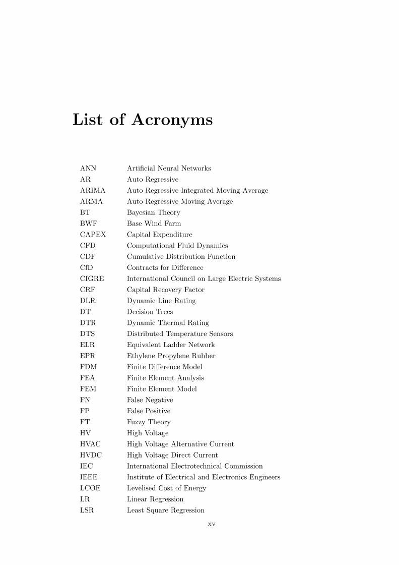
List of Acronyms
ANN Artificial Neural Networks
AR Auto Regressive
ARIMA Auto Regressive Integrated Moving Average
ARMA Auto Regressive Moving Average
BT Bayesian Theory
BWF Base Wind Farm
CAPEX Capital Expenditure
CFD Computational Fluid Dynamics
CDF Cumulative Distribution Function
CfD Contracts for Difference
CIGRE International Council on Large Electric Systems
CRF Capital Recovery Factor
DLR Dynamic Line Rating
DT Decision Trees
DTR Dynamic Thermal Rating
DTS Distributed Temperature Sensors
ELR Equivalent Ladder Network
EPR Ethylene Propylene Rubber
FDM Finite Difference Model
FEA Finite Element Analysis
FEM Finite Element Model
FN False Negative
FP False Positive
FT Fuzzy Theory
HV High Voltage
HVAC High Voltage Alternative Current
HVDC High Voltage Direct Current
IEC International Electrotechnical Commission
IEEE Institute of Electrical and Electronics Engineers
LCOE Levelised Cost of Energy
LR Linear Regression
LSR Least Square Regression
xv

xvi
MA Moving Average
MAD Median Absolute Deviation
MAE Mean Average Error
MC Markov Chain
MCMC Markov Chain Monte Carlo
MCS Monte Carlo Simulation
MERRA Modern-Era Retrospective Analysis for Research and Applications
MV Medium Voltage
NOAA National Oceanic and Atmospheric Administration
NWP Numerical Weather Predictions
OHL Over Head Lines
PCR Principal Component Regression
PDF Probability Distribution Function
PE Polyethylene
PLS Partial Least Squares
QR Quantile Regression
QRF Quantile Regression Forest
RC Resistor-Capacitor Circuit
RF Random Forest
RMSE Root Mean Square Error
RTTR Real-Time Thermal Rating
RTU Remote Terminal Unit
SCADA Supervisory Control and Data Acquisition Unit
SL Single Lead
SVM Support Vector Machine
SVR Support Vector Rgression
TEE Thermo Electric Equivalent
TN True Negative
TOR Thermal Overload Risk
TP True Positive
TPM Transition Probability Matrix
TRE Thermal Risk Estimation
TSO Transmission System Operators
VAR Vector Auto Regressive
WF Wind Farm
WFO Wind Farm Overplanting
WPC Wind Power Curtailment
WT Water Temperature
XLPE Cross-Linked Polyethylene

List of Symbols
Wc Conductor loss (W)
Ws Sheath loss (W)
Wa Armour loss (W)
Wd Dielectric loss(W)
W Heath source (W)
T Thermal resistance (K.m/W)
C Thermal capacitance (J/K)
ys Skin effect
Rac Conductor a.c. resistance at 90C (Ω/m)
Rdc Conductor d.c. resistance at 90C (Ω/m)
λ′1 Eddy current loss
λ′′1 Circulating current loss
λ1 Ratio of losses in the metal sheath with respect to the conductor(s) losses
Rs Resistance of the sheath per unit length of cable at 90C (Ω/m)
ω Angular velocity
X Sheath reactance per unit length (Ω/m)
s Distance between conductor axes (mm)
d Mean diameter of the sheath (mm)
I Current in one conductor (A)
λ2 Ratio of losses in the armour with respect to the conductor(s) losses
RA Resistance of the armour at 90C (Ω/m)
dA Mean diameter of the sheath (mm)
c Distance between conductor axis and the cable centre (mm)
f Voltage frequency in (Hz)
Cd Capacitance per unit length in (F/m)
tanδ Dielectric loss factor Tangent value
4θ Increment of conductor temperature above ambient temperature (K)
θ Node temperature in cable thermal network
n Number of load-carrying conductors in the cable
Uo Phase voltage
p Van wormer coefficient
P Transition probability matrix
xvii

xviii
∆M Ramp event magnitud
∆t Ramp event duration
P Wind farm power output (W )
Vref Reference voltage (V )
Θ Power factor
Is Static cable rating (A)
IB Base wind farm maximum output current (A)
Imax Wind farm maximum output current (A)
Tlimit Maximum cable operating temperature (C)
Te Estimated conductor temperatures, MCS based TRE method (C)
Tr Realistic conductor temperatures, MCS based TRE method (C)
r Risk of cable overheating, MCS based TRE method [0-1]
r Realistic risk of cable overheating, MCS based TRE method [0-1]
R′ Risk of cable overheating, MC based TRE method [0-1]
R Realistic risk of cable overheating, MC based TRE method [0-1]
T ′c Estimated conductor temperatures, MC based TRE method (C)
Tc Realistic conductor temperatures, MCS based TRE method (C)
erisk Risk of cable overheating, Ramp Identification based TRE method [0-1]
rrisk Realistic risk of cable overheating, Ramp Identification based TRE method [0-1]
T ′ Estimated conductor temperatures, Ramp Identification based TRE method (C)
T Realistic conductor temperatures, Ramp Identification based TRE method (C)

Acknowledgements
Firstly, I want to thank my Mexican sponsor CONACYT- SENER who made possible
for me to come to the University of Southampton to perform my doctoral studies. I
was lucky to receive advice and help from Dr Ruben Salas Cabrera and Dr Jonathan
Mayo Maldonado during the transition from my Masters in Mexico to PhD in the United
Kingdom for which, I am truly thankful.
Secondly, I would like to express my sincere gratitude to Dr James Pilgrim for accepting
me under his supervision and giving me the opportunity and trust to develop this re-
search. Arriving in the United Kingdom in 2015 was a life-changing and overwhelming
experience which I started enjoying when I found the right path and this exciting project
under your supervision. Thank you for the knowledge shared, the guidance, patience
and, for believing in me even when I was not believing in myself.
Thirdly I want to thank Dr Orestis Vryonis whose support and loving advice have helped
me throughout my last year of PhD and during the writing period of this thesis.
Additionally, I would also like to mention my friends and colleagues in the Electrical
Power Engineering group and my friend Maria Rosca because during our lunch breaks
or tea talks you have made me smile and recharge my batteries before getting back to
work.
Finally my dad Jose Edilberto Hernandez Vazquez, my mom Margarita Colin Garcia,
my sister Luz Aurora Hernandez Colin and my dog Camila who have always been with
me even in the distance. Thank you for your prayers, thoughts and, words of support
which were the primary motor of my strength.
Thank you.
xix


Agradecimientos (Espanol)
En primer lugar, quiero agradecer a mis patrocinadores, CONACYT-SENER, que hicieron
posible que viniera a la Universidad de Southampton para realizar mis estudios de doc-
torado. Tuve la suerte de recibir consejos y ayuda del Dr. Ruben Salas Cabrera y
del Dr. Jonathan Mayo Maldonado durante la transicion de mi Maestrıa en Mexico al
Doctorado en el Reino Unido, por lo cual estoy realmente agradecida.
En segundo lugar, me gustarıa expresar mi sincero agradecimiento al Dr. James Pilgrim
por aceptarme bajo su supervision ası como brindarme la oportunidad y confianza para
desarrollar este trabajo de investigacion. Llegar al Reino Unido en 2015 fue una experi-
encia abrumadora y transformadora que comence a disfrutar cuando encontre el camino
correcto y este interesante proyecto bajo su supervision. Gracias por el conocimiento
compartido, la orientacion, la paciencia y por creer en mı, incluso cuando yo no creıa en
mı misma.
En tercer lugar, quiero agradecer al Dr. Orestis Vryonis, cuyo apoyo y amorosos consejos
me han ayudado durante mi ultimo ano de doctorado y durante el perıodo de redaccion
de esta tesis.
Tambien me gustarıa mencionar a mis amigos y colegas en el grupo de Ingenierıa de En-
ergıa Electrica y a mi amiga Maria Rosca porque durante nuestros almuerzos y platicas
me han hecho sonreır y recargar las baterıas antes de volver al trabajo.
Finalmente mi papa Jose Edilberto Hernandez Vazquez, mi mama Margarita Colın
Garcıa, mi hermana Luz Aurora Hernandez Colın y mi perra Camila que siempre han
estado conmigo incluso en la distancia. Gracias por sus oraciones, pensamientos y pal-
abras de apoyo, que fueron el motor principal de mi fuerza.
Gracias.
xxi


Chapter 1
Introduction
The offshore wind industry in the United Kingdom (UK) generated 8% of electricity
demand in 2018, which covered the energy needs of 6.9 million homes, and it is aimed
to cover 10% of electricity demand by 20201. The increased competition for projects
development led to a 50% reduction in energy prices since 2015 according to the contracts
for difference (CfD) auction in 20172 while a further 30% reduction over this reduced
prices was confirmed in the CfD auction in September 20193. As a consequence, there
is an increased interest in the optimisation of the overall performance of the wind farm
installation to further reduce the cost of offshore energy generation.
This thesis is focused on the optimisation of current rating in submarine power cables.
Given that, export cables represent a significant percentage of the capital expenditure
(CAPEX) of an offshore wind farm, the optimisation of cable rating/size is an essential
part of project optimisation [1].
1.1 Submarine Power Cables
Submarine power cables are major transmission cables carrying electric power beneath
the ocean in the voltage range of 35 kV - 800 kV. They are used to carry electric power
beneath the ocean, making possible to transfer offshore wind power back to shore and
perform network interconnections between countries. The two options for high voltage
(HV) power transmission are high voltage alternating current (HVAC) and high voltage
direct current (HVDC) cables, for which the main selection criteria are route length,
voltage and need for grid synchronisation.
HVAC is the preferred option for short-distance transmission, typically for routes of
less than 100 km, while HVDC is used for longer distance transmission [2]. HVDC
1www.gwec.net2www.gov.uk/government/publications/contracts-for-difference-cfd-second-allocation-round-results3www.gov.uk/government/publications/contracts-for-difference-cfd-allocation-round-3-results
1

2 Chapter 1
transmission cables are cheaper and have limited losses however, their main disadvantage
is the high losses in DC converters as well as higher prices, compared to AC transformers.
As a consequence, the use of HVAC cables is more economically attractive when allowed
by the overall system length. The main limitation for AC cables is that as transmission
distance increases, the amount of reactive power (charging current) in the cable also
increases, thus reactive compensation devices across the line need to be installed.
Modern transmission systems were developed using AC rather than DC given that AC
currents can be raised or lowered employing transformers to reduce Joule losses. Con-
sequently, most offshore export cables in the UK are HVAC systems, however, as wind
farms distance from shore increases, DC transmission becomes a competitive alternative
to AC transmission.
The typical HVAC offshore export cable consists of three insulated conductors in a trefoil
formation placed into a single underwater cable structure for voltages up to 150 kV [3]
while mostly single-core cables are used above this voltage. The main characteristic in
offshore export cables is a concentric armour most often built using steel wires which
reinforces the structure to avoid damage to the cable. Figure 1.1 presents the cross-
sectional area of a typical 3 core single lead (SL) type submarine HVAC power cable.
The work in this thesis is limited to HVAC offshore wind farm export cables with cross-
linked polyethylene (XLPE) insulation and operational temperature limit of 90C [4].
Figure 1.1: Cross sectional area of 3 core HVAC submarine export cables.4
4http://ritmindustry.com/catalog/cables-for-electric-power-supply-and-power-distribution/power-distribution-cable-multi-conductor-shielded-subsea/

Introduction 3
1.2 Power Cable Ratings
The amount of power that a cable can carry is limited by the insulation material which
would face an accelerated ageing process if operated at temperatures higher than 90C
[5]. The second factor limiting the ampacity of the cable are the thermal properties of
the surrounding environment whose ability to dissipate the heat generated by the current
circulating in the conductors plays an essential role in the thermal rating problem.
The most widely accepted method to calculate power cable ratings is the use of the static
rating calculations, IEC60287 [6], which has been used in operation for over four decades.
Continuous rating equations are deliberately conservative calculation that estimates the
maximum amount of current that can be carried by the conductor without reaching
or exceeding the limiting temperature of the insulation. Although these calculations
are easy to perform the assumptions of fixed worst-case weather parameters around the
cable systems often lead to underutilisation of the carrying capacity of the cables [7].
In reality, a submarine cable circuit would never operate at its maximum current rating
continuously and without power fluctuations. Furthermore, weather parameters are
continuously varying around the cable system i.e. ambient, water or soil temperatures,
moisture content, burial depth and soil types change across the route [8].
The alternative to the use of static rating calculations is the use of dynamic/real-time
rating calculations, which make use of measurement devices or nearby weather stations to
approximate the environmental conditions in real-time and calculate cable ratings based
on the actual conditions experienced by the cable system. Dynamic rating methodologies
have been successfully applied in many cases in conventional installations on land to
increase the amount of load in a cable from 5% to 15% compared to static ratings [7].
1.3 Offshore Wind Farm Overplanting
Static ratings applied to offshore wind farm export cables often lead to under-utilisation
of real cable capacity [9] because the assumption of a continuous rating is far away from
the intermittent power generation faced by the cable which along the cable long thermal
time constant generates low cable temperatures. The concept of Wind Farm Overplant-
ing (WFO) is the deliberate increment of installed wind generation capacity over the
conservative continuous rating of the cable [10]. The extra installed capacity is meant
to capture more energy at low wind speeds thus, reducing the effective transmission cost
per turbine, making the project more cost-effective [1].
Nowadays, WFO has become a common practice in the offshore wind farm industry in
the UK, however, loading the cable over the conservative continuous rating limits could
introduce the possibility of exceeding the cable temperature limits. Some of the existing
4 Chapter 1
over-planting increments apply modest capacity increments to avoid exceeding the cable
limiting operational temperature.
Another existing practice is the application of Wind Power Curtailment (WPC) which
is a reduction in the wind farm power output when high wind speeds generate full power
over long durations. WPC can be applied by the transmission system operator (TSO)
via automatic or manual signalling to shut down certain wind turbine generators to
reduce the output power and allowing the cable to reduce its temperature.
The installation of distributed temperature sensors (DTS) inside newly developed sub-
marine cables helps to perform cable temperature monitoring and can be used as a
security tool to generate instantaneous alerts against thermal overheating.
However, the use of instantaneous alarms and curtailment strategies could be optimised
by the generation of hours ahead information of the cable thermal state. For instance,
knowledge of the future cable thermal state some hours ahead could help to perform
planing of power curtailment when WFO is applied to prevent thermal damage to the
cable system while avoiding unnecessary power curtailment.
1.4 Research Motivation
Submarine power cables connecting wind farms to onshore substations are often sized
considering static rating calculations as is traditionally done with cables on land. How-
ever, unlike slow and predictable load variations as in conventional installations, in
offshore wind farms, the amount of power transferred through the cable is a product
of wind speed variations and thus the load in the cable can vary significantly in short
amounts of time. As a consequence, for the offshore cable scenario, the application of
historically conservative ratings along with long cable thermal time constants leads to
highly underestimated ratings.
Dynamic/real-time rating calculations measure or estimate environmental conditions
around the cable to calculate the actual permissible load current in the cable. In conven-
tional installations, real-time ratings allow the operator to increase power transmission
however, in the offshore case scenario it is necessary to develop a methodology that can
account for uncertainty in future wind power generation.
Wind farm overplanting has recently been used in the offshore industry to increase
the capacity utilisation of export cables [10]. However, to safely increase the cable
ratings employing WFO, it is necessary to account for uncertainty in the cable load
some hours ahead and performing an estimation of the future cable temperatures taking
into account the cable thermal dynamics. Thus, a simulation tool/decision-making tool
that estimate thermal risk some hours ahead based on historical data can help to improve
the application of WFO by reducing unnecessary wind power curtailment.
Introduction 5
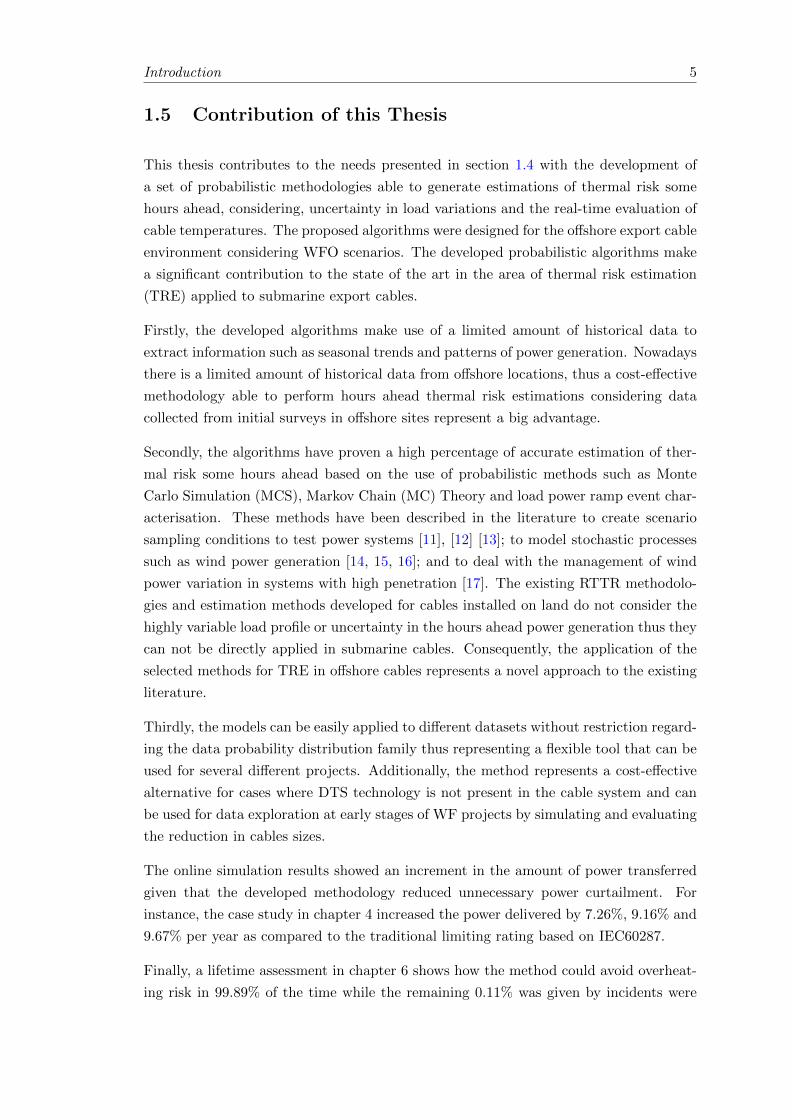
1.5 Contribution of this Thesis
This thesis contributes to the needs presented in section 1.4 with the development of
a set of probabilistic methodologies able to generate estimations of thermal risk some
hours ahead, considering, uncertainty in load variations and the real-time evaluation of
cable temperatures. The proposed algorithms were designed for the offshore export cable
environment considering WFO scenarios. The developed probabilistic algorithms make
a significant contribution to the state of the art in the area of thermal risk estimation
(TRE) applied to submarine export cables.
Firstly, the developed algorithms make use of a limited amount of historical data to
extract information such as seasonal trends and patterns of power generation. Nowadays
there is a limited amount of historical data from offshore locations, thus a cost-effective
methodology able to perform hours ahead thermal risk estimations considering data
collected from initial surveys in offshore sites represent a big advantage.
Secondly, the algorithms have proven a high percentage of accurate estimation of ther-
mal risk some hours ahead based on the use of probabilistic methods such as Monte
Carlo Simulation (MCS), Markov Chain (MC) Theory and load power ramp event char-
acterisation. These methods have been described in the literature to create scenario
sampling conditions to test power systems [11], [12] [13]; to model stochastic processes
such as wind power generation [14, 15, 16]; and to deal with the management of wind
power variation in systems with high penetration [17]. The existing RTTR methodolo-
gies and estimation methods developed for cables installed on land do not consider the
highly variable load profile or uncertainty in the hours ahead power generation thus they
can not be directly applied in submarine cables. Consequently, the application of the
selected methods for TRE in offshore cables represents a novel approach to the existing
literature.
Thirdly, the models can be easily applied to different datasets without restriction regard-
ing the data probability distribution family thus representing a flexible tool that can be
used for several different projects. Additionally, the method represents a cost-effective
alternative for cases where DTS technology is not present in the cable system and can
be used for data exploration at early stages of WF projects by simulating and evaluating
the reduction in cables sizes.
The online simulation results showed an increment in the amount of power transferred
given that the developed methodology reduced unnecessary power curtailment. For
instance, the case study in chapter 4 increased the power delivered by 7.26%, 9.16% and
9.67% per year as compared to the traditional limiting rating based on IEC60287.
Finally, a lifetime assessment in chapter 6 shows how the method could avoid overheat-
ing risk in 99.89% of the time while the remaining 0.11% was given by incidents were
6 Chapter 1
the cable temperature exceeded the allowed 90C by less than 0.5C. These results cor-
respond to a WFO of 9.9% above the static cable rating along with the developed TRE
method in chapter 4.
1.5.1 Key research aspects
To the best of the author’s knowledge, a methodology that can generate a quantita-
tive risk of cable temperature exceedance for offshore wind farm cables has not been
developed. Thus, the proposed research can contribute towards the development and
application of non-static rating methodologies in submarine cables to optimise the cable
installation capacity. The novel aspects that are considered in this work are listed below:
• The probabilistic algorithms are based on a limited amount of historical data to
perform hour ahead thermal risk estimations in submarine power cables.
• The developed methodology can avoid unnecessary power curtailment on cables
under WFO scenarios which increases the power delivered compared to traditional
static rating limits.
• Wind farm export cable optimisation can help to decrease the cable contribution
to the LCOE in offshore installations.
• The method could be applied to different wind farm locations and cable sizes given
the necessary data from the site.
• The algorithm can represent a helpful tool for simulation and planning when the
data from initial surveys in offshore locations is collected to optimise cable sizing.
1.6 Report Structure
This chapter describes the research questions and motivation of this thesis. The intro-
duction to the problem starts by describing the main difference between cables on land
and offshore as well as the limitations of the existing cable rating methodologies when
applied to offshore cables. Additionally, the importance of cable rating optimisation to
reduce the levelised cost of energy was explained. Finally, the main contributions of the
thesis are outlined along with a list of the novel aspects that this research adds to the
current literature on hours ahead TRE in offshore export cables.
Chapter 2 starts with an analysis of the thermal rating problem in submarine power
cables considering the cable design and construction. An overview of the thermal heat
sources in the cable and an introduction to the standard equations in IEC60287 and
IEC60853 along with its limitations and assumptions are presented. The alternative

Introduction 7
numerical methodologies for cable rating calculations are described along with its ad-
vantages and disadvantages over analytical methods. The chapter continues with a
summary of relevant cable rating methodologies, probabilistic methods, statistical tech-
niques and its limitations to be applied in the offshore wind farm scenario is presented.
Finally, the methodologies applied in wind speed and wind power forecasting are anal-
ysed with a focus on the selected forecasting/estimation methodologies selected for the
investigation.
Chapter 3 presents the firstly developed probabilistic forward thermal risk estimation
methodology based only on MCS analysis. The results consider 5, 10 and, 18 years of
training data, 1 year of testing data, and 6, 12 and, 24 hours ahead estimation windows.
The exploration performed in this chapter considered 3 WFO cases and the financial
benefit analysis of using the proposed methodology compared to the use of static rating
limitations. The methodology and results presented in this chapter were published and
presented in the international conference on Probabilistic Methods Applied to Power
Systems (PMAPS).
Following the results and conclusions obtained from the probabilistic methodology pre-
sented in Chapter 3, the use of Markov Chain theory along MCS analysis was explored
considering 1st and 3rd order MC models. The proposed Markov based forward TRE
methodology is presented in Chapter 4 along with the generated results and a results
comparison regarding the pure probabilistic TRE methodology in Chapter 3. The MC
based methodology and results presented in this chapter were published in a journal
paper in the IEEE Transactions on Power Delivery.
Chapter 5 proposed an alternative TRE method based on the analysis of historical wind
power ramp events to identify and anticipate its thermal consequences for the cable. The
proposed approach makes use of clustered analysis of load current ramp rates gathered
from historical data to identify ramp events and perform an hours ahead estimation
of thermal risk in the cable given the identified ramp direction and intensity. The
ramp identification framework and results presented in this chapter were submitted as
a journal paper in the IEEE Transactions on Power Delivery and are under review at
the moment of submission of this thesis.
Given the additional power transmission that was achieved by using the proposed TRE
algorithms, an explanatory financial benefit analysis is presented in Chapter 6. Addi-
tionally, a lifetime analysis (20 years simulation) was carried out to evaluate the eco-
nomic benefits of the application of WFO and the proposed online Markov Chain TRE
method. The analysis in this chapter also presents the comparison of economic benefits
considering water temperature variations.
Finally, chapter 7 summarises the results and contributions of the work presented and
future development options for the developed TRE methodologies.


Chapter 2
Polymeric AC Submarine Power
Cables and Rating Methods
This chapter presents the general construction of polymeric HVAC submarine cables
and the thermal rating problem faced in these cables. Additionally, the IEC standard
equations used to calculate the maximum rating of submarine and land cables are in-
troduced along its assumptions and well-known limitations.
The chapter continues with the description of the numerical methodologies used in the
literature as an alternative to the analytical equations.Relevant real-time/dynamic rating
methodologies found in the literature are analysed along the probabilistic and statisti-
cal methods used. Finally, existing methodologies related to hours ahead cable rating
estimations as well as wind power/ramp forecasting are analysed with a focus on the
selected methods for this purpose.
2.1 Submarine Cable Design
The structural design of a submarine power cables must have a strong mechanical resis-
tance, high transmission capacity and insulation efficiency. The fundamental difference
in the design between land power cables and submarine power cables is an armour layer
which protects the cable core from water pressure, wave currents and the natural forces
affecting the underwater environment which strength varies with depth. For instance the
deeper the cable is installed the lower the water temperatures, water pressure increase
and wave effects are diminished.
Additional structural elements such as lead sheath and insulating screens are used for
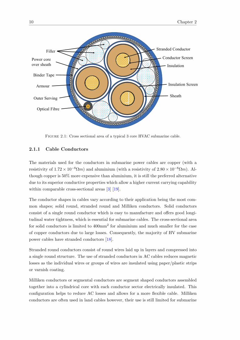
water blocking as well as abrasion and corrosion resistance. The elements in the design
of a submarine power cable are shown in Figure 2.1 and will be further explained in this
section based on technical details from [3],[18] and [19].
9
10 Chapter 2
Stranded Conductor
Conductor Screen
Insulation Screen
Insulation
Sheath
Power core
over sheath
Outer Serving
Filler
Binder Tape
Armour
Optical Fibre
Figure 2.1: Cross sectional area of a typical 3 core HVAC submarine cable.
2.1.1 Cable Conductors
The materials used for the conductors in submarine power cables are copper (with a
resistivity of 1.72× 10⁻⁸Ωm) and aluminium (with a resistivity of 2.80× 10⁻⁸Ωm). Al-
though copper is 50% more expensive than aluminium, it is still the preferred alternative
due to its superior conductive properties which allow a higher current carrying capability
within comparable cross-sectional areas [3] [19].
The conductor shapes in cables vary according to their application being the most com-
mon shapes; solid round, stranded round and Milliken conductors. Solid conductors
consist of a single round conductor which is easy to manufacture and offers good longi-
tudinal water tightness, which is essential for submarine cables. The cross-sectional area
for solid conductors is limited to 400mm2 for aluminium and much smaller for the case
of copper conductors due to large losses. Consequently, the majority of HV submarine
power cables have stranded conductors [18].
Stranded round conductors consist of round wires laid up in layers and compressed into
a single round structure. The use of stranded conductors in AC cables reduces magnetic
losses as the individual wires or groups of wires are insulated using paper/plastic strips
or varnish coating.
Milliken conductors or segmental conductors are segment shaped conductors assembled
together into a cylindrical core with each conductor sector electrically insulated. This
configuration helps to reduce AC losses and allows for a more flexible cable. Milliken
conductors are often used in land cables however, their use is still limited for submarine
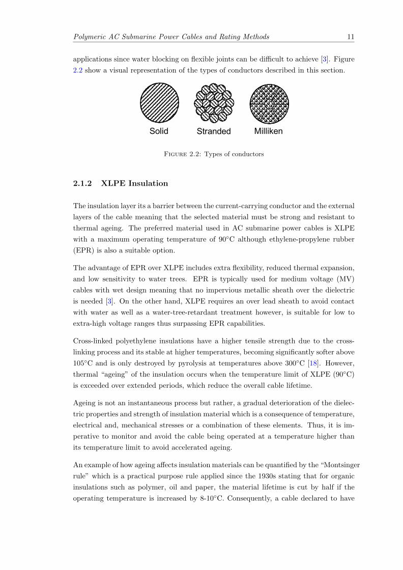
Polymeric AC Submarine Power Cables and Rating Methods 11
applications since water blocking on flexible joints can be difficult to achieve [3]. Figure
2.2 show a visual representation of the types of conductors described in this section.
!"#$% !&'()%*% +$##$,*)
Figure 2.2: Types of conductors
2.1.2 XLPE Insulation
The insulation layer its a barrier between the current-carrying conductor and the external
layers of the cable meaning that the selected material must be strong and resistant to
thermal ageing. The preferred material used in AC submarine power cables is XLPE
with a maximum operating temperature of 90C although ethylene-propylene rubber
(EPR) is also a suitable option.
The advantage of EPR over XLPE includes extra flexibility, reduced thermal expansion,
and low sensitivity to water trees. EPR is typically used for medium voltage (MV)
cables with wet design meaning that no impervious metallic sheath over the dielectric
is needed [3]. On the other hand, XLPE requires an over lead sheath to avoid contact
with water as well as a water-tree-retardant treatment however, is suitable for low to
extra-high voltage ranges thus surpassing EPR capabilities.
Cross-linked polyethylene insulations have a higher tensile strength due to the cross-
linking process and its stable at higher temperatures, becoming significantly softer above
105C and is only destroyed by pyrolysis at temperatures above 300C [18]. However,
thermal “ageing” of the insulation occurs when the temperature limit of XLPE (90C)
is exceeded over extended periods, which reduce the overall cable lifetime.
Ageing is not an instantaneous process but rather, a gradual deterioration of the dielec-
tric properties and strength of insulation material which is a consequence of temperature,
electrical and, mechanical stresses or a combination of these elements. Thus, it is im-
perative to monitor and avoid the cable being operated at a temperature higher than
its temperature limit to avoid accelerated ageing.
An example of how ageing affects insulation materials can be quantified by the “Montsinger
rule” which is a practical purpose rule applied since the 1930s stating that for organic
insulations such as polymer, oil and paper, the material lifetime is cut by half if the
operating temperature is increased by 8-10C. Consequently, a cable declared to have
12 Chapter 2
a 30 years lifetime if operated at 90C, could double its lifetime service if operated at
80-82C [18].
2.1.3 Conductor Screen and Insulation Screen
The triple-extrusion insulation is complemented by a conductor screen placed onto the
conductor and an insulation screen over the insulation wall, together (conductor screen-
XLPE insulation-insulation screen) these layers form the dielectric cable system.
The conductor screen helps to reduce local electrical stress in the insulation due to
any surface irregularities in the conductor material, thus providing a smooth transition
towards the dielectric wall. On the other hand, the insulation screen is used to assure
a uniform electric field within the insulation. The screens material is semiconducting
XLPE, based on polyethylene (PE) polymers blended with 40% carbon-black, with a
nominal thickness between 1-2 mm [18].
2.1.4 Cable Water Barrier
The cable water barrier is formed by the water blocking tape, the sheath, and the power
core over-sheath. The polymeric water blocking tape or swelling tape is a water-absorbing
agent placed over the insulation screen which can keep the insulation dry enough from
any humidity making its way through the sheath.
The radial water-barrier sheath/metallic screen is most commonly built with an extruded
lead alloy which also acts as a metallic screen that provides a ground potential to carry
capacitive and fault currents.
Finally, the power core over-sheath is a watertight anticorrosion cover that partially
avoids water diffusing through the sheath while also providing mechanical support for
the structure below. Thus, the jacket is sized to keep the water vapour going through
within appropriate limits.
2.1.5 Filler and Binder Tape
The gaps between the trefoil formation of the power core over-sheath are filled with
a soft material such as polypropylene yarn which withstands high temperatures while
providing flexibility. The main role of filler material in the cable structure is to keep the
structure round.
Binder tapes are made out of polyester fibres placed onto the underlying cable structure
in a spiral shape with a typical overlap of 25-50%. Fillers and binder tape provide

Polymeric AC Submarine Power Cables and Rating Methods 13
stability, roundness and, a smooth surface which protects the cable from the armour
abrasive forces.
2.1.6 Armour
The cable armour layer is the most distinctive element in submarine power cables, it
is a prominent layer whose main purpose is to provide mechanical protection, tensional
strength, and stability. Submarine cable armours are often built from circular galvanised
steel wires which are wound around the cable in a lay angle which combined with the
conductor’s lay angle and anti-twist tape achieve a “torque balance” that prevents the
cable from twisting under torsional forces [3].
The lay/pitch length of the armour wires help to support tensional forces expected
for the cable such as the impact of cable weight during installation, or external haz-
ards throughout cable service life.Thus, the laying angle is optimised according to the
tensional forces expected for the cable. Large pitch lengths increase the cable tensile
stability and strength however, as lay length increases so do the bending stiffness which
may be undesirable [18], [3].
Finally, submarine armoured cables must be protected against corrosion caused by ma-
rine saltwater, the common practice is the application of a primary zinc layer of 50µm
thickness over the steel wires while a second protection layer of hot bitumen finishes the
corrosion protection[18].
2.1.7 Outer Serving
The cable outer serving is made from one or more layers of polypropylene yarn applied
over the armour. It helps to protect the anti-corrosion layers from abrasion while sta-
bilising the cable structure and providing a neat surface wish is also rough enough to
provide a good grip during installation [18].
The laying direction of the yarn strings follows the direction of the underlying armour to
prevent the yarn strings to be torn apart by the torsional movement of armour wires. Fi-
nally, the colour of the outer serving material is generally black with longitudinal stripes
of a different colour, such as yellow, to provide visibility during and after installation.
2.1.8 Optical Fibres
Nowadays submarine power cables are being equipped with optical fibres placed outside
the power core over-sheath inside the filler material as shown in figure 2.1. Optical fibres
are used for data transmission and temperature measurement along the cable length.

14 Chapter 2
Distributed temperature sensing (DTS) devices can monitor cable temperature based on
the detection of the back-scattering of light via Rayleigh, Raman or Brillouin principles.
Typical accuracy figures of DTS devices are on the range of ±1C with 1 meter spatial
resolution [20].
DTS has been used to estimate the soil thermal properties in underground cable instal-
lations [21] and was able to locate hot spots of faults along the cable as seen in [22].
Based on the measurements of cable temperatures along the line, ampacity increments
can be safely performed for the case of underground cable systems [23].
2.2 The Thermal Rating Problem
During operation, the load current in power cables will lead to heat dissipation from
the conductor to the outer layers of the cable and into the surrounding environment.
Thus, the cable rating depends on the balance between the heat generated in the ca-
ble and the heat dissipated. For instance, the maximum static rating calculation is
given by the amount of load current that the cable can carry without exceeding the
limiting temperature of the insulating material, on the assumption of constant ambient
conditions.
The current rating (also called ampacity) calculation in cables, has been widely detailed
in textbooks [19] and summarised in the international industrial standards IEC 60287[6]
and IEC 60853[24] established for the calculation of static and transient calculations.
The standard equations facilitate the calculation of cables ampacity covering a wide
range of AC and DC cables designs, installation conditions, and cable voltages (up to 5
kV for DC).
2.2.1 Heat Sources Within the Cable
The main heath sources/losses within the cable are conductor Wc, sheath Ws, armour
Wa and dielectric losses Wd. The Joule losses in the metallic parts are dependent on the
load current circulating in the conductor and the material’s resistance.
2.2.1.1 Conductor Losses
The conductor losses Wc are generated due to the electrical a.c. resistance of the con-
ductor which is temperature dependent and affected by the magnetic field caused by
the AC current and proximity of adjacent conductors. Wc is, for instance, the most
significant source of joule losses in the cable.

Polymeric AC Submarine Power Cables and Rating Methods 15
The a.c conductor resistance is influenced by the skin effect (ys), and the proximity
effect (yp) factors, the skin effect is caused by the magnetic field in the conductor which
reduce the useful conductor area by pushing the current density away from the conductor
centre, thus, as the current density across the conductor becomes less uniform and the
effective a.c. resistance increases.
The proximity effect factor is influenced by the distance between the conductors in
three-phase AC cables. Given that, the magnetic field of the other conductors forces
the current path far away from the adjacent conductor the current density becomes
inhomogeneous. The calculation of the conductor a.c. resistance at 90C is then given
by
Rac = Rdc(1 + ys + yp) [Ω/m] (2.1)
where Rdc is the conductor d.c. resistance at 90C and the factors ys and yp are calcu-
lated as per IEC 60287 equations [6]. The joule losses are then calculated as
Wc = I2Rac [W ] (2.2)
where I is the current flowing in one conductor (A). It must be noted that the armour
layer in cables increases the skin and proximity effects thus, a factor of 1.5 should be
added for its calculation which is not clearly stated in the IEC standard.
2.2.1.2 Sheath Losses
The sheath losses Ws appear due to the alternating magnetic field around the conductor
which generates losses named: eddy (λ′1) and circulating currents (λ′′1). Eddy losses are
loops of current produced within the sheath due to the magnetic flux lines of alternating
current penetrating into the sheath, see Figure 2.3.
Metallic Sheath Sheath Bonding
Eddy Currents
Circulating Currents
Figure 2.3: Eddy and circulating currents in metallic sheaths

16 Chapter 2
Circulating losses are produced by induced currents flowing along the metallic sheath
to the earth bonding and returning through another conductor sheath, thus, circulating
currents exist only when the sheaths of the three-phase cable are bonded at both ends
as is the common case for submarine cables. The calculation of sheath losses is given by
Ws = λ1I2Rac [W ], (2.3)
where the power loss factor λ1 = λ1′+λ′′1. However, as the two currents superpose along
the sheath, eddy losses are neglected (λ′′1 = 0) when circulating currents are present [6].
For the case of three-core cables which each core has a separate lead sheath (SL-type
cables) the IEC standard 60287 defines the loss factor λ1′ as
λ′1 =Rs
Rac· 1.5
1 +
(Rs
X
)2 (2.4)
where Rs is the resistance of the sheath per unit length of cable at 90C in (Ω/m); ω =
2π× f ; X is the sheath reactance per unit length (Ω/m) given by X = 2ω10−7ln
(2s
d
);
s is the distance between conductor axes (mm) and; d is the mean diameter of the sheath
(mm).
The calculation of equation 2.4 as per IEC60287-1-1 assumes uniform current density
flowing in conductors and sheaths, however, the authors in [25] demonstrates that such
assumption does not hold for large 3-core export cables due to conductor proximity
effects. The results in [25] evidenced that the current calculation of λ1 as per [6] generates
an overestimation of up to 7C (8%) for cables with large conductor sizes.
2.2.1.3 Armour Losses
Armour losses Wa are caused by hysteresis and eddy current losses generated due to
the alternating magnetic field around the cable conductors. Hysteresis losses occur
due to magnetisation and demagnetisation of the armour wires as current flow in both
directions. The increment and decrement of the flux density in the steel wires does not
occur at the same rate thus creating hysteresis loops which in essence is energy wasted
in the form of heat. Eddy currents are also generated in the armour layer as explained
for the case of the sheath.
The calculation of the armour losses as per IEC60287-1-1[6] is defined by the equation
Wa = λ2I2Rac [W ] (2.5)

Polymeric AC Submarine Power Cables and Rating Methods 17
where the armour loss factor λ2 for SL-type cables is defined as
λ2 = 1.23RA
Rac
(2c
dA
)2
· 1(2.77RA106
w
)2
+ 1
·(
1− Rac
Rsλ′1
)(2.6)
being RA the resistance of the armour at 90C in (Ω/m); dA is the mean diameter of the
sheath (mm); c is the distance between the axis of the conductor and the cable centre
(mm).
The factor λ′1 in equation 2.6 is obtained from IEC 60287-1-1 (2.3.1) as follows
λ′1 =Rs
Rac
1
1 +
(Rs
X
)2 . (2.7)
It is important to state that equation 2.6 is currently under consideration as several
studies have found that it overestimates the armour losses [26] [27] specially on large ca-
bles such as 3-core submarine cables [28] [29]. Correction of the armour losses equations
sugested by IEC 60287 will substantially decrease the conductor sizes for the case of sub-
marine cable systems in the future, however, it is out of the scope of this investigation
to deal with the errors regarding λ1 and λ2.
2.2.1.4 Dielectric Losses
Finally, the heat losses generated in the dielectric material Wd depends not on the
current but the phase voltage (Uo). Due to the dielectric imperfections, small currents
are allowed to flow and charge to accumulate within the dielectric which acts as a
capacitor. The calculation of the dielectric losses is given by
Wd = 2πfCdUo2tanδ [W ] (2.8)
where f is the voltage frequency in (Hz); Cd is the capacitance per unit length in (F/m)
and; tanδ is the tangent value of the dielectric loss factor.
2.3 Cable Rating Calculations
The calculation of cable ratings employing analytical methods/empirical equations is
summarised in the IEC standards 60287 and 60853. IEC standards are widely accepted
for the calculation of static, transient and emergency ratings in onshore and offshore
cable systems.

18 Chapter 2
The alternative to the standards is the use of numerical methods such as finite difference
method (FDM), finite element method (FEM) and computational fluid dynamics (CFD)
which can handle more realistic environmental situations and consider time-dependent
load profile variations for arbitrary study cases [3].
Analytical and numerical methods are summarised in the following sections starting
by the equations in the IEC standards, its assumptions, advantages and disadvantages.
The description of the most popular numerical/computational methods used for cable
rating calculations compared to IEC standards for the case of submarine cables is also
analysed.
2.3.1 Analytical cable rating calculations: IEC standards
The analytical equations in the IEC standards are based on the Neher-McGrath method
published in [30] and [31] which described the procedure to solve the thermal rating
problem based on the analogy of the different layers of a cable represented as resistors
and capacitors while the heat losses in the cable Wc,Wd,Wa and Ws are represented as
current sources.
The thermo-electric representation of cables allow the calculation of ratings considering
the heat generated in the cable and the heat dissipated from the cable. The cable network
includes the surrounding environment as part of the electric circuit where heat flowing
through the layers of the cable is analogous to the current flowing through resistors and
capacitors.
Given that, the network of a cable system can be very complex to solve using analytical
methods, the IEC standards use an equivalent thermal network of the cable were the
reduced circuit consist of two loops representing the internal and external layers of the
cable system [19].
2.3.1.1 IEC standard 60287-1 & 2: Static cable ratings.
The steady-state/continuous rating of a cable is defined as the amount of current that
a cable can carry without exceeding the maximum operating temperature of the cable.
The first part of the IEC standard 60287-1 [6] contains the analytical equations for the
calculation of the permissible current rating of a.c. and d.c. cables, buried or in air
conditions. The permissible current rating of a.c. buried cables is calculated as
I =
[4θ −Wd[0.5T1 + n(T2 + T3 + T4)]
RT1 + nRac(1 + λ1)T2 + nRac(1 + λ1 + λ2)(T3 + T4)
]0.5(2.9)
where T1, T2, T3 and T4 are the thermal resistances between the one conductor and the
sheath, between sheath and armour, from the outer covering and between the cable

Polymeric AC Submarine Power Cables and Rating Methods 19
surface and the surrounding soil, respectively, given in (K.m/W ); 4θ is the increment
of the conductor temperature above ambient temperature (C), and n is the number of
load-carrying conductors in the cable.
The second part of the standard IEC60287-2 [32] contains the necessary equations to
calculate the thermal resistance of the different layers of the cables (T1, T2, T3 and T4).
For the calculation of the thermal resistance of the surrounding soil, the standard con-
siders the different installations of cables e.g. free air, buried cables groups of cables
and cables in pipes. The well-known assumptions and limitations of the IEC standard
equations are discussed in subsection 2.3.1.3.
2.3.1.2 IEC standard 60853-2: Cyclic and emergency ratings.
The calculation of cyclic and emergency ratings of power cables are covered in the IEC
standard 60853-2 [24]. Section one of the standard studies the transient temperature
response of cables to a step function using the lumped thermal circuit of the cable system
representing the internal and external cable environment. The two partial transients
θc(t) and θe(t) are calculated separately and then sum to obtain the total temperature
rise θ(t) of the cable above the temperature in the external environment.
The second section in the IEC standard 60853-2, is concerned with the calculation of
cyclic ratings. Here, a daily profile of load is included in the rating calculations to
obtain the maximum peak current allowed in 24 hours period. The procedure for the
calculation of the cycling rating factor (M) by which the steady-state current I must be
multiplied is explained in the standard.
Finally, in the third section, the calculation of emergency ratings is addressed. An
emergency rating is defined as a current carried for a short period (e.g. 1, 3, 6 hours)
before the cable reaches its maximum operating temperature. This rating is calculated
through the application of a step load I2 > I for a time t after the steady-state conditions
of the system are reached.
2.3.1.3 IEC general assumptions.
The analysis of the cables in the IEC standards 60287 and 60853 consider general as-
sumptions such as
• Consideration of constant load in the cable system (IEC60287);
• 1D analysis assumption of no heat flowing longitudinally;
• Thermal resistivity and diffusivity of the soil are assumed constant;
• Worst-case weather/environmental parameters are used for the rating calculations;
• The cable burial depth is assumed constant in IEC equations;

20 Chapter 2
In reality, cable systems face variable load currents, drying out of the soil, variable
weather/soil parameter; hot spots along the cable line (longitudinal heat variations).
Fixed worst-case conditions and the restrictions considered in the standards produce
the continuous and transient ratings to be conservative [7]. However, these assumptions
make the standard calculations simple and fast to perform which is the main reason why
the standard calculations are widely used.
For the case of submarine power cables, burial depth changes across the route due to
sand wave migrations also occur thus, for the offshore wind scenario, the application of
IEC60287 rating method along with highly variable load currents and long cable thermal
transients leads to underestimated ratings and underutilisation of cable capacity.
2.3.1.4 IEC limitations for SL-type submarine armoured cables.
In the case of 3-core SL-type, armoured, submarine power cables, it’s been evidenced in
[26] and [33] that the calculation of the armour losses λ2 using the IEC 60287 produces
overestimated values which leads to even more conservative ratings. In this thesis, the
armour losses are calculated as per IEC equations for all the study cases.
The specific case of a submarine cable design is not addressed in the IEC standard,
however, the SL-type representation of buried cables is accepted on industrial prac-
tices for the sizing and rating calculation in offshore cables. Nevertheless, as previously
mentioned, the consideration static load currents are far away from reality given the
variability of wind power generation profiles.
Furthermore, the work in [34] analyse some issues regarding the reduction of the cable
thermal network of the case of SL-type cables in the IEC two-loop cable representation
which present errors. For instance, Figure 2.4 presents two network single-core repre-
sentations of an SL-type three-core cable for which the IEC standard two-loop circuit
gives the equations in (2.10).
TA = T1;
TB = qsTf + qaT3; (2.10)
QA = Qc + pQi
QB = (1− p)Qi +Qs + 0.5Qf
qs+
(qaT3
qsTs + qaT3
)2(0.5Qf
qs+Qa +Qj
qa
)where T symbolise thermal resistances; Q thermal capacitances; subscripts 1,2 and 3
represent the insulation, armour bedding and serving; subscripts s, f, a and j symbolise
sheath filler armour and jacket layers; p is the van wormer coefficient [6]; λ1 and λ2 are
the sheath and armour loss factors; qs = 1 + λ1 and qa = 1 + λ1 + λ2.

Polymeric AC Submarine Power Cables and Rating Methods 21
Figure 2.4: Two equivalent single-core network representations for the SL-type 3-corecable (from [34])
The IEC equivalent equations in 2.10 supposedly assume: 1) the conductor losses are
equal to the total Joule losses in the 3 conductors; 2) the thermal resistance between
conductor and screen is one-third of the original 3-core cable and; 3) the capacitances of
conductor, insulation and, screen is 3 times the original. However, to correctly represent
the 3-core SL type cable under the assumptions above the two-loop equations in the
IEC standards should be modified as in 2.11 as found by the analysis presented by G.
Anders et. al. in [34].
TA = T1;
TB = 3(qsTf + qaT3); (2.11)
QA = Qc + pQi
QB = (1− p)Qi +Qs +Qf/6
qs+
(3qaT3
qsTs + 3qaT3
)2(Qf/6
qs+Qa +Qj
3qa
)
Additionally, to the correction in the two-loop representation of the SL-type cable, which
is the actual option in the IEC standards when modelling submarine cables, the authors
in [34] introduce a novel equivalent network representation specifically for the most
common construction of a 3-core SL-type armoured submarine cable with jacket around
each core which is the cable model adopted in this study and is presented in detail in
Section 3.4.
2.3.2 Numerical Cable Rating Methods
The use of numerical methods as an alternative to the analytical rating equations became
popular with the advent of powerful desktop computers. The most common numerical
methods used to solve cable rating problems are; finite difference method (FDM)[35],

22 Chapter 2
finite element method/analysis (FEM/FEA)[36],[37] and computational fluid dynamics
(CFD)[38]. Numerical models can deal with complex problems where the assumptions
of the IEC standards would lead to underestimated rating.
The shared operational principle of numerical methods is the discretisation of partial
differential equations representing the layers of the cable and surrounding environment
(solution area). A series of interconnected nodes or a mesh across the cable geometry
are used to discretise the thermal rating problem. The main difference between these
methods is how the interconnections nodes are treated for each numerical approach.
The use of computational models allows the study of cables considering non-homogeneous
soil conditions[39], the variation of burial depth [36], moisture migration[40], variable
load current profiles and, complex cable installations studies[37] which are some of the
general assumptions considered in the standards to reduce the rating problem complex-
ity.
2.3.2.1 Finite Difference Method
The finite difference method calculates the temperature at each cable layer considering
the adjacent node in a one dimensional (1D) analysis. The partial differential equations
of the cable nodes are approximated by a linear combination of functions based on the
Taylor series principle.
FDM has been used in real-time applications where rating calculations have to be up-
dated at a specific time interval [35]. The relatively fast computational time of FDM
compared to other numerical methods is its main advantage while it has been demon-
strated that the accuracy of the temperature calculations are in agreement with those
obtained from IEC standard equations when isothermal boundary conditions are as-
sumed [39].
2.3.2.2 Finite Element Method
Although the principle of the finite element method is similar to FDM the mathematical
techniques used in FEM to describe the relationship between the nodes in the cable
geometry (mesh) are more flexible and can be applied to complex cable installation and
geometries.
FEM models can handle non-linearity and can be used to analyse two (2D) and three
dimensional (3D) cable systems environments. For instance, the author in [39] used
2D and 3D finite-difference models to demonstrate that when including burial depth
variations for shallowly buried cables the IEC standard calculations led to overestimated
ratings for the case of land cables. Additionally, the works in [36] and [37] presents the

Polymeric AC Submarine Power Cables and Rating Methods 23
development of 2D and 3D FEM models for the thermal rating calculation of water-
cooled joint bays and J-tubes respectively. The numerical FEM models allowed for a
more realistic study of the installation conditions experienced by cable joints and J-tubes
in service.
The number of elements in which the studied cable is divided as well as the dimen-
sional solution space (2D/3D) increments the FEM computational time. For the case
of 2D models, it can be minutes while for 3D models finding a solution can take several
hours. Nevertheless, the precision and accuracy of FEM methods are widely used as a
benchmark for the validation or comparison of newly developed methodologies that deal
with the calculation of faster and more detailed transient temperature models for cables
[41],[42].
Finally, it must be considered that for simple cable installations the use of the standard
equations produces almost the same results compared to FEA models [43],[44] in those
cases, the additional computational complexity must be avoided.
2.3.2.3 Computational Fluid Dynamics
Computational Fluid Dynamics is a 3D form of finite-difference analysis used to describe
fluid flow problems in cases where the cable is installed in direct contact with air or water.
CFD is applied along a FEM of the cable for cases where the cable is in air-filled troughs
or tunnels, however, CFD applications are considered complex problems especially when
involving turbulent airflows.
The authors in [38] developed a CFD model to study rating increments in HV cables
circuits installed in naturally ventilated troughs. The numerical model was compared
to the IEC equations traditionally used for the case of covered unfilled troughs, which,
is not directly addressed by the standard. The results found that the continuous rating
of the cable could be increased by 28% given the natural convection reducing the air
temperature around the cable.
2.4 Dynamic Cable Rating Methodologies and Commer-
cial Software
Real-time rating systems have been successfully installed in buried cables, cables in
ducts, tunnels and overhead lines to maximise the asset utilisation of such systems. A
combination of direct or indirect ambient parameters and the application of analytical
and numerical methodologies is found in the literature to estimate cable ratings mostly
in overhead and underground systems.

24 Chapter 2
Data acquisition devices such as thermocouples, optical fibres (DTS), remote terminal
units (RTUs), sag tension monitoring devices, meteorological stations are some of the
devices used to collect real-time temperature, weather and current data used for the
real-time rating calculations [45][20].
Developed real-time rating methods for the calculation of static, transient and emergency
ratings are found in the literature, i.e. MAXAMP [46], CYMCAP[47], DTCR [48] and
DCRS[49]. These algorithms are mostly based in Neher-Mc.Grath, IEC 60287 and IEC
60853 standards.
2.4.1 MAXAMP
A dynamic feeder rating system (DRF) installed in a complex tunnel installation is de-
scribed in [46]. The MAXAMP method can perform real-time, steady-state, emergency
cable rating calculations and overload duration times without exceeding the cable maxi-
mum operating temperature. MAXAMP cable designs include single-core and three-core
cables installed in air, directly buried, submarine, ducts and tunnels based on the Mc-
Grath equations, IEC 60287 and IEC 60853 standards.
The cable models are based on the thermoelectric equivalent principles thus the multi-
loop ladder networks of the cables in [19] are used while considering enhancements
to take into account measured load current and cable/ambient temperatures obtained
employing thermocouples or fibre optics.
Additional features of the DFR are remote communication, storage of historical data over
24 hours, alarm capabilities, voltage levels of 5-500kV, overhead and underground cable
installation models. Finally, the algorithm can perform a 1300 min rating estimation in
the future based on the previous 24h load current cycle and the Brent’s roots algorithm.
2.4.2 CYMCAP
A similar computer program named CYMCAP is presented in [47] which is also based
on Neher-McGrath and IEC Standards equations and can be used for cables in pipes,
directly buried or in a thermal backfill, underground ducts and duct banks. The cable
design library includes single-core, three-core, belted, pipe-type, submarine, sheathed,
and armoured cables.
The CYMCAP computational algorithm features a user-friendly interface and virtual
representations of the underground cable models and installations mentioned above.
This characteristic makes it easy for the user to modify and enrich the model’s library.
The solution techniques are based on the iterative solution of IEC standards for the
calculation of static ratings, ampacity, given time and cable temperature, temperature

Polymeric AC Submarine Power Cables and Rating Methods 25
analysis, given time and actual rating and, time to reach a given temperature, considering
actual cable rating.
The similarities between MAXAMP and CYMCAP relate also to its limitation for direct
application to submarine export cable systems. Although the submarine cable design
based on the IEC equations of an SL-Type cable can be modelled by this software the
use of measurement devices in submarine cables is limited. DTS technology, if installed
in the cable system, can generate cable temperature measurements every 5 minutes to
calculate the static and emergency ratings.
Nevertheless, for the studied offshore cable scenario, the variable load current is not
driven by demand but subject to available generation. Thus, instantaneous static or
emergency ratings do not consider the uncertainty in future power generation.
2.4.3 EPRI Dynamic Rating System DTCR
Examples of computational algorithms that can perform hours ahead estimation of cable
ratings are DTCR [48] and DCRS [49] software. The calculations of the EPRI software
are based on ANSI/IEEE standard equations and are design to perform dynamic rating
calculation on overhead lines underground cables and power equipment such as power
transformers, current transformers, switches, bus, line, and circuit breakers.
The software features the ability to avoid dependency on temperature measurement
devices thus calculation of cable and equipment temperatures are solely based on real-
time weather and load current data. The software calculates a real-time thermal rating,
a maximum static rating, long term (1-24 hours) and short term (5 to 60 minutes)
emergency ratings.
The input variables for the DTCR algorithm are hourly weather/soil and load current
data which must be available in a 24 hours ahead period to perform the temperature
and rating calculations. The estimation of load current must be obtained by the user
and could be based on conservative typical values, or based on historical data from the
operational centre.
2.4.4 Dynamic Cable Rating Systems DCRS
The software DCRS [49] features an online and offline calculation of steady-state and
dynamic cable ratings as well as forecasting rating for overhead and underground cables.
The input variables to the algorithm are real-time cable load, cable surface temperature,
ambient temperature and a weather forecast.
The methodology uses the relevant cable model which is constructed according to the
cable specifications using the thermoelectric analogy principles while a computational

26 Chapter 2
algorithm solves the ordinary differential equations using the Runge-Kutta method to
solve for node temperatures.
The offline application of DCRS can be used by the system operator to understand
the dynamic characteristic of the cable system while the online algorithm can gener-
ate steady-state ratings, cable temperature, a forecast of future cable temperature and
available ampacity.
2.4.5 Alternative Dynamic Rating Methodologies
The cable rating method presented in [50] is an enhanced version of the lumped pa-
rameters model which are the base of the IEC standards. The developed thermoelectric
equivalent (TEE) models are compared to FEM simulations, and the obtained tem-
perature calculations are within 1.5 C allowing fast and accurate real-time rating cal-
culations. The method proved to be accurate for steady-state analysis and to some
extent for dynamic rating calculations by the subdivision of cable components, however
compromising calculation times.
A second example is given by the electro-thermal coordination (ETC) approach in [50]
which is introduced as an operation and planning strategy based on the temperature of
the transmission system components instead of the current load. Dynamic temperature
calculations in a 2×100km long cable line system were obtained using a TEE [41] model
of the system components allowing a 50% current increment on the cable over the static
rating with no risk of exceeding the limiting operation temperature.
Additionally, the knowledge of the instantaneous temperature allowed to foresee the
evolution of the transmission system due to known cable load patterns and it was found
that the load increment could be kept for up to 3 days without generating thermal risk
in the cable. Nevertheless, the application of the methodology in [50] by itself can not be
directly used in an offshore wind farm cables as it does not account for the uncertainty
of future load current in the cable.
The RTTR method described in [51] can compute predictions of cable heating and load
capacity using measured temperatures provided by monitoring systems. The thermal
model of the cable system is based on the modelling and optimisation of an equivalent
ladder network (ELN) of the cable system studied which is afterwards solved by FEM.
The optimisation of the cable model minimises the deviation of the temperature profile
by comparing simulated and measured temperature values which allow for automatically
consideration of drying out of the soil and external heat sources in the final model.
Alternative methodologies to target optimisation of specific features such as the optimal
representation of soil characteristics [52] or the transient thermal behaviour of mutual
heating effect when dealing with buried cables [42] have been developed based on the

Polymeric AC Submarine Power Cables and Rating Methods 27
adaptation of the equivalent ladder network approach. The RC thermal ladder-type
model equivalent model in [52] was tested [53] and the obtained temperature calculations
were compared to FEM simulations with an accuracy of 0.5 C and 20 times faster which
is imperative when dealing with dynamic rating calculations.
A great number of methodologies combine the use of temperature sensors and other
monitoring devices and the existing standard equations to calculate the rating of over-
head lines [54] [55] [56] and underground cable systems [22] and [53]. The complexity of
the methodologies varies regarding the needs and attributes targeted.
One example is the low-cost sensing probe consisting of LM35 temperature sensors and a
GPRS transmitter which was developed and tested for dynamic line rating calculations
[56]. The device was tested in a 400V and 11 kV overhead distribution line and was
able to measure temperature data used to determine the real-time line rating based just
on standard IEEE and IEC equations. The simplicity and affordable cost in this work
resulted in an average increment in line capacity of about 25%.
More complex systems considering monitoring devices such as RTU’s, meteorological
stations, conductor temperature/load current sensors and radiation monitors are used
in [54] and [55] for the on-line rating calculation of rating in overhead lines. The main
disadvantage in the approaches would be the added cost of the device installation, main-
tenance, and additional monitoring equipment. On the other hand, the monitoring of
the overhead line is indispensable when applying DLR as overhead conductors have
fast transients and the amount of environmental parameters affecting the cable thermal
rating is greater [57].
Although the enhancements in TEE and RTTR methods can be used in the cable model
for the case of submarine cables in order to improve rating accuracy, they are indepen-
dent of any estimation methodology. In other words, the alternative dynamic rating
methods by themselves would not be of much help for the case of hours ahead ther-
mal risk estimation thus suitable probabilistic algorithm to represent and estimate the
uncertainty of future load must be used.
2.4.6 Application of the Existing Algorithms for Offshore WF Cable
Rating.
The real-time software and methodologies in this section represent a helpful planning
tool for conventional installations where the load follows slow-changing cyclic patterns.
However, in offshore export cables, knowledge of the real-time and future cable temper-
ature is needed to allow rating increments above static limits without overheating the
cable.

28 Chapter 2
In conclusion, despite the successful application of the existing algorithms in conventional
installations, similar benefits can not be obtained in an offshore wind farm application
because:
• The load current in an overhead/underground cable can be based on previous system
demands in a cyclic and seasonal basis while the load in a submarine power cable is
generated by the wind which is random by nature and varies in short periods.
• A real-time rating would not produce the required information for the system operators
to know if the hours ahead load profiles could generate overheating in the cable system.
• The availability of measurement devices along the line as well as the meteorological
stations needed by some of the above algorithms are not available in offshore cable sites.
For instance, meteorological weather stations, as well as wind speed and power forecasts
offshore, are very limited.
Table 2.1 summarises the input parameters and measurement devices needed to be
installed/available around the cable systems where the real-time rating software is to be
deployed.
Software Input Parameters and Measurement Devices
MAXAMP • Considers load current, cable surface temperature
[46] from RTUs, DTS, and thermocouples.
• Soil thermal resistivity is updated every 24h.
CYMCAP • Considers load current and cable temperature
[47] measured from the SCADA system.
DTCR • Considers load current, weather data and equipment
[48] parameter data from the SCADA system, 24 ahead load current
24 hours ahead weather forecast data.
DCRS • Considers cable loading, cable temperature, ambient temperature,
[49] and a forecasting of weather parameters. Obtained from line sag,
tension and temperature monitors + meteorological stations.
Table 2.1: Commercial dynamic rating softwares overview.
2.5 Cable Rating Estimation and Forecasting Methods
The existing methods for estimation and forecasting of overhead/underground cable rat-
ings have been developed considering pure probabilistic methodologies based on weather

Polymeric AC Submarine Power Cables and Rating Methods 29
data or historical data i.e.[11],[12] while other hybrid methodologies make use of mea-
sured or estimated parameters combined with statistical methods i.e.[58].
The cable rating estimation algorithms in the literature make use of probabilistic method-
ologies such as Monte Carlo Simulations (MCS)[59], [11],[12],[60] , Bayesian theory (BT)
and Markov Chain (MC) models [61],[62]; regression analysis models such as Partial
Least Squares [63],Support Vector Regression (SVR)[64] or Quantile Regression[65], [66].
The use of machine learning techniques such as Artificial Neural Networks (ANN)[67],[68]
and Fuzzy Theory (FT) [69] was also found for the estimation of overhead/underground
ratings. However, regression methods, as well as machine learning algorithms, require
large data sets to generate regression coefficients and hidden learning networks which
usually remain fixed thus ignoring the uncertainty nature of weather conditions affecting
the cable rating.
Additionally, the need for large quantities of data to improve accuracy is a limiting factor
considering the lack of data for offshore locations. Consequently, only MCS, BT and MC
are considered as suitable methods to represent the uncertainty of weather conditions
using a short amount of historical data.
2.5.1 Monte Carlo Simulation (MCS)
Monte Carlo Methods are the class of computational algorithms used to obtain numeri-
cal results for deterministic problems by the repeated random sampling and evaluation
of experiments. The underlying principle of randomness states that individual random
events lack pattern or predictability however, the frequency of the outcomes over nu-
merous events is predictable.
The use of MCS is seen in a wide number of fields such as finance, energy industries,
manufacturing, engineering and research using probability distribution functions (PDFs)
to describe variables. MCS is found applied to optimisation problems, numerical integra-
tion, and random sampling draws from probability distribution functions. Examples of
MCS used in power systems are found applied to reliability analysis [70], risk assessment
[71], system stability [72], and numerous dynamic rating estimations approaches.
The system variables are represented by distribution functions containing the set of pos-
sible values and its corresponding likelihood obtained from the set of data. By using
PDFs and an MCS, different sets of values are drawn from the probability distribution
functions representing a finite number of simulated experiments (probabilistic scenar-
ios) which the system could experience given random combination of parameters. The
advantages of MCS over deterministic methods is the ability to generate probabilistic

30 Chapter 2
results showing not only what could happen but also how likely the events are. Ad-
ditionally, scenario analysis, variable correlation studies and sensitivity analysis can be
easily performed using MCS.
Historical weather data measured around a cable system and MCS were used in [59],
[11], [12] and [13] to estimate PDF’s of conductor temperature. Probability distribution
functions were used to represent parameters such as load data, soil thermal resistivity
and ambient temperature for different types of installations such as overhead lines, un-
derground cables, pipe cooled and forced cooled cables systems. The evaluation of the
randomly generated values was used to calculate steady-state ratings and estimate the
likely temperature probability distribution function of the cable system.
The methodology in [59] makes use of probability distribution functions of load current,
backfill/ soil thermal resistivity and ambient parameters obtained from load demand
records, historical weather records. The Monte Carlo technique was used along with the
developed FEM algorithm to evaluate cable temperature under different combinations
of system parameters. A probability distribution function of conductor temperatures
was obtained after a sufficient number of simulations. The information generated by the
methodology in [59] helped the system operators to understand if the studied system
could handle an increased load, for instance, results showed up to 50% available room
for load increment in a pipe type underground cable system.
The work in [11] describes a methodology developed to determine the optimal rating
increment for a 32-year-old buried cable system. Probability density functions for load
current, ambient temperature and soil thermal resistivity were obtained by statistical
analysis of historical data of August, the most critical month for the circuit studied. The
MCS procedure selected random inputs from the PDFs which were evaluated using stan-
dard methods. As in the previous example after a “sufficient” number of repetitions the
cable temperature distribution function was obtained. The analysis of the most critical
cable temperatures helped the system operators to estimate that a cable rating could
be increased by 32% under normal operating conditions with a maximum temperature
of 80C.
The applied methodology in [12] follow the same sampling and evaluation procedure
described in [59] and [11] for the case of a pipe cooled underground cable system. The
study involved the use of load current and ambient temperature PDFs while the thermal
analysis of the cable at each iteration in the MCS was performed using a FEM of the
studied cable. Similarly to [11] the most critical months for the cable system were
analysed (July and December) under a 20% 30% and 40% increased load current and
the probabilistic method was used to obtain the PDF of cable temperatures. Results
showed that a 20% load increment could be safely implemented considering both critical
months with a maximum cable temperature of 90C.
Polymeric AC Submarine Power Cables and Rating Methods 31
The probabilistic tools in [59], [11] and [12] were developed to simulate increments of
load in the cable system considering past seasonal data. Nevertheless, these approaches
are not able to estimate hours ahead cable rating or temperature which is necessary for
the offshore export cable scenario.
Conversely, the work in [60] and [13] features an algorithm capable of generating cycling
rating forecasts for planning purposes. Emergency and cyclic rating forecast up to 6
hours ahead were based on MCS and monthly PDF of ambient temperature, cooling
data, water temperature, soil thermal parameters and the nominal load demand curves
for the studied circuit. The sampled ambient parameters and the actual load of the
system were evaluated with a pice-wise equation for rating calculations to building a
cumulative distribution of conductor temperatures from which the likely probability
exceeding the cable temperature limit was obtained.
The methodology in [13] can be applied for several kinds of cable installations such as;
free air, troughs, buried, naturally cooled or artificially cooled. The validated results
confirmed that the methodology could increase the rating of a cable system up to 44%
with a 12% likelihood of exceeding its temperature limit for a buried cable system. The
main restriction for the application of this algorithm in the offshore case scenario is its
dependency on the knowledge of the cyclic demand load curves which is not the case
for an offshore export cable were the load in the cable is based on random wind speed
variations, thus, based on available generation instead of on user demand.
The study in [58] proposed the use of a weather forecast and a state estimation technique
to calculate cable rating forecast some hours ahead for the case of an overhead line. The
study features the use of weather parameter forecasts from the National Oceanic and
Atmospheric Administration (NOAA) to build probability distribution functions which
are sampled using MCS and feed into a thermal model of the cable. The MCS pro-
cess samples evaluate the hours ahead of weather parameters and generate a minimum,
maximum and mean average cable rating. The obtained conductor temperature PDF
helped to perform rating improvements between 8 MVA and 43 MVA over the 90 MVA
summer static rating of the line for up to 24 hours horizon.
Several variables can be considered when using MCS, however, the inclusion of pa-
rameter correlations such as the selection of low current values associated with high
ambient temperature values and vice versa was stated as an important characteristic to
achieve accuracy in the conductor temperature estimations by generating more realistic
scenarios[11]. This characteristic was also found in [58] for the case of wind direction,
air temperature and solar radiation values when performing the Monte Carlo Sampling.
Additionally, when representing variables using probability distribution functions (PDFs)
the selection of the distribution function must fit the real data to increase results pre-
cision. For example, the most common distribution for ambient temperature is the
Gaussian distribution while Weibull distribution is widely accepted to represent wind

32 Chapter 2
velocity [73]. Flexible distribution shapes such as the Beta distribution and Kernel dis-
tribution to fit data are the alternative to the selection of parametric distribution which
can generate errors due to fixed used defined shape parameters [74].
2.5.2 Bayesian Theory
Probability, according to the Bayesian approach, is interpreted as a reasonable expec-
tation or quantification of belief instead of the frequency or propensity of an event.
Bayesian probability is defined by accounting for the available information (prior distri-
bution) and when more information become available the Bayes’ formula (2.12) is used
sequentially to calculate the posterior distribution which in turn becomes the next prior.
The mathematical formulation of Bayes’ theorem is given by
P(A | B)=P(B | A)P(A)P(B)
(2.12)
where A and B represent events, given that P(B) 6= 0, the likelihood of the event A
occurring is P(A | B). The probability P(B | A) is also a conditional probability that
represents the likelihood of B occurring given that A is true; while P(A) and P(B) are
individual probabilities.
The use of Bayesian theory has been used for the hours ahead estimation of weather
parameters which are in turn used to calculate cable ratings and risk of temperature
exceedance. For instance, an online calculation of dynamic line rating in [61] and [62]
use a combination of load monitoring and historical weather data of previous days to
estimate a 1 hour ahead thermal overload risk (TOR) for an overhead line. The prior
probability distributions of weather parameters (built considering historical data) are
used to estimate a posterior distribution of weather parameters and decide the next hour
rating. As new data arrives the prior distributions become the posterior, and the model
is updated.
Results in [62] presented the 1 hour ahead thermal risk along with the proposed line
rating given the calculated TOR. For instance, considering the actual line rating as
1471A the next hour TOR was calculated as 72.4% and the proposed reduced rating
was 1335.96A to avoid exceeding the temperature limit of the line.
Although in the case of an overhead line the weather variables affect greatly the cable
rating, in the offshore case scenario considering underwater variables the case is not
the same. For example, water temperature changes can affect the cable rating, but,
they do not vary in the same way as wind speed or sun radiation in an overhead cable.
In consequence, the TOR obtained from the algorithm in [62] for the offshore case
scenario would not represent a great advantage given that uncertainty in the load current

Polymeric AC Submarine Power Cables and Rating Methods 33
generation and cable thermal dynamics must be taken into account hours ahead in order
to help the TSO in planning and decision making.
2.5.3 Markov Theory
Markov models are based on the statistical analysis of data to extract probabilistic
patterns in the form of Transition Probability Matrices (TPM). The studied system
output variable is divided in a finite number of system states which are used to calculate
the probability of change of the variable from one state at time t to another state at
t + 1. A time-series analysis of the data is used to calculate all the states probabilities
to form the Transition Probability Matrices of the system. TPM’s can then be used to
estimate the most likely future values that the variable can attain based on its actual
value.
For example, consider the system variable (I) an a defined number of system states (q)
such that Q = 1, 2, . . . q thus, the probability of transition from state i to state j is
defined as
pij = pI(t+1) = qj | I(t) = qi, ∀i, j ∈ 1, 2, . . . , q. (2.13)
The individual transition probabilities pij for each system state are obtained from the
historical data analysis as (eq. from [75])
pij =historical transitions of qi → qjhistorical transitions of qi → Q
, (2.14)
to form the elements of the TPM (P) such that
P =
p11 . . . p1q...
. . ....
pq1 . . . pqq
. (2.15)
The obtained one-step TPM can estimate the most probable state of the system at time
t + 1 considering the actual state at time t only and its called Markov Chain. The
successive powers of the TPM i.e. Ph result in the calculation of the most probable
state at time t+ h and are call higher-order Markov models.
Following the process for the calculation of the first-order TPM in (2.13) where the
estimation of state t+ 1 depends only on the state at time t, in a third-order MC-TPM
the transition probabilities pij are calculated as
pij = pI(t+1) = qj | I(t) = qi, I(t−1) = qj, I(t−2) = qk, ∀i, j, k ∈ 1, 2, . . . , q (2.16)

34 Chapter 2
where the probability of the load current state at time t+1 depends on the analysis of the
states at t, t−1 and t−2. The study of additional past data values i.e.t−3, could improve
the accuracy of the estimations however, the complexity of the TPM calculation will be
increased which would require higher computational times and computer capabilities.
Depending on the number of states in the system the size of P increases i.e. q system
states generates a q by q matrix. Additionally, the first order TPM in (2.15) considering
the analysis in (2.13) estimates the future state t+1 depending only on the state at time
t however, higher-order TPM can be created considering additional past data values i.e
t− 1,t− 2,t− 3. Higher-order TPM could improve the accuracy of the estimations how-
ever the additional complexity would require higher computational times and computer
capabilities.
The application of Markov models was not found for cable rating calculations, however,
the principles described above were found in the literature to model stochastic variables
and generate probabilistic forecasts of wind speed [76], wind farm generation [75, 77]
and power demand forecasting [14, 15, 16] applications.
The wind power forecasting method in [75] describes the process of creating a first and
second order MC model for wind power forecasting. The results compared the use of 1st
and 2nd order MC models which achieved similar forecasting results for a 10 minutes
ahead window due to the highly variable nature of the studied data. The amount of
data used for the models in [75] and [77] is 2 years divided in training and testing sets
and it can be studied monthly or seasonally as in [77] to model the capture the power
generation patters for the particular season.
Another application of MC theory is seen in [16] and [15] where the objective is the de-
velopment of an energy consumption forecast on a daily/weekly basis using one year of
historical data. The resulting energy forecasts were compared to Artificial Neural Net-
works and it was found that the estimation errors using a Markov Chain model could
be reduced when incrementing the number of system states [16]. The calculated error
between the measured data CDF (cumulative distribution function) and the forecasted
data (CDFerror) was 4.1% for the MC model and 4.9% for the ANN which demonstrates
that MC models can generate accurate load predictions whit-out the unnecessary com-
plexity of an ANN.
In conclusion, the main advantages of using Markov models is that they are purely
statistical thus they have no restrictions regarding probability distributions of data. In
other words, transition matrices are built based on the studied data and the same model
can be used in different sets of data from different geographical locations.

Polymeric AC Submarine Power Cables and Rating Methods 35
2.5.4 Wind Power Generation Forecasting
A great number of papers investigate wind energy forecasting for the case of onshore wind
turbines i.e. [78],[15],[79],[80],[81],[82] and [83] while the works related to offshore sites is
still limited [84],[85] due to the relatively new interest in offshore wind farm projects. The
general steps for the generation of a wind power forecast are; the wind speed prediction;
the calculation of the output power using the selected wind turbine power curve and;
finally, the upscaling or downscaling of the estimations for the geographic region studied
[86],[87].
The forecasting methods found in the literature can be divided into statistical ap-
proaches, based only on the study of wind data and the physical approaches, based
on a detailed modelling of the terrain characteristics and atmospheric parameters. Nev-
ertheless, the combination of the two has also been applied [88],[89],[90]. The pure
statistical approaches have been identified as easy to model, inexpensive, and accurate
enough [87] because they are based on patterns found in historical data over a specific
period of time.
The statistical methods found in the literature applied to wind power forecasting include;
Moving Average (MA), Auto Regressive Moving Average (ARMA), Auto-Regressive In-
tegrating Moving Average and Markov Chain models [15],[79],[75],[83], Markov Switch-
ing Autoregressive Models [84], Markov Chain Monte Carlo (MCMC) [82]. Machine
learning methods such as Artificial neural networks [85], Support Vector Machine (SVM),
K-nearest neighbours [91] and Fuzzy models which are also based on the analysis of data
area popular alternative [92],[93].
Although, wind power forecasting could be seen as a suitable approach to follow when
aiming to perform an hours ahead cable thermal rating estimation, there exist particular
problems found in the literature when performing wind generation prognostics. For
instance, the cubic relationship between power and wind speed has been identified as
the main source of errors in forecasts given that a small wind prediction error generates
a large power output error [87].
Additionally, it has been found that wind speed changes in an offshore environment have
a stronger impact in the wind turbines generation due to the flatness of the environment
[92],[94] thus the available meteorological models used in onshore methodologies cannot
be directly applied in offshore sites.
Given that the objective of this project is the cable thermal risk estimation and its
management, the errors generated by a wind power forecasting approach involving wind
speed prediction and power output calculation would be avoided. Instead, the present
study makes use of a historical load current profile to directly estimate hours ahead load
current scenarios avoiding accumulated power output errors.

36 Chapter 2
The methodologies suggested for wind forecasting on land are varied and goes from
simple moving average models to machine learning algorithms, however, the application
of these techniques for offshore locations is still unknown given the higher wind variations
and limited knowledge of the meteorological wind patterns offshore.
According to the analysis of the relevant literature, Markov models seem to be suit-
able algorithms to deal with wind power production data onshore and offshore as they
can represent and model probabilistic transitions and fluctuation of various magnitudes
that can not be modelled using explanatory variables. For instance, the work in [84]
suggests a Markov Switching Autoregressive model forecast offshore wind power fluc-
tuations, while several authors have tested MC models for wind power forecasting on
land [15],[79],[75],[83]. Markov models are then seen as the most suitable method to be
adapted for thermal risk estimation of offshore wind farm cables.
2.5.5 Wind Power Ramp Forecasting
Large and fast wind power variations are the main drawback characteristic of wind en-
ergy sources, thus, their integration to the network has brought the necessity to develop
new ways of predicting energy swings to manage supply and demand. The study of
ramp events is based on the idea that large and fast power variations are critical enough
to be targeted separately rather than focusing on the full wind power forecasting profile,
see [17].
The related literature evidence that the definition of ramp event has not been strictly
formulated however, is generally characterised by a magnitude (∆M), duration (∆t),
ramp rate (∆M/∆t) and direction (±). Similarly, the criteria for ramp identification
and classification has not been generalised thus, several approaches are proposed in
the literature going from a binary classification (ramp/no ramp) to more sophisticated
methods [17].
The starting step identified in the related works is the definition of a threshold value
(th) which draws the line for the identification of a ramp event. The threshold th can
be expressed as a percentage of installed capacity or as an absolute power magnitude
and its selection must be agreed with end-users according to the case studied because
the underlying behaviour or ramps is a case dependent problem.
Additionally, due to the novelty of the topic, there is still no agreement on how to
approach or evaluate ramp events. For instance, ramp event alarms, on-line ramp iden-
tification/detection, forecasting of ramp rates and probabilistic ramp event occurrence
methods are seen in the literature [95].
The majority of wind power ramp event methods is focused on the study of onshore wind
power systems to help reliability issues in power grid operations, intelligent distribution,

Polymeric AC Submarine Power Cables and Rating Methods 37
electric grid management and future smart grid market mechanisms [17]. For example,
a ramp detection algorithm which analyses and extracts ramp parameters is seen in [96]
where a classification framework with ramp rules and scoring functions identifies wind
ramps from a large time series.
The characterisation framework was well established, however, no attempt to forecast
ramps or perform real-time recognition was made as done in [97] where an online recog-
nition method is presented. The work in [97] establishes a ramp model where an event
consists of several linear wind power variation segments from which the ramp rate and
future power are derived from the detected amplitude and duration.
Examples of methodologies for wind power ramp forecasting were also found based
on machine learning algorithms such as neural networks [98] support vector machines
[99] and hybrid SVM-Markov Chain enhanced model [78]. These classification-based
algorithms analysed wind power data to predict the class or per unit (p.u.) value of
power fluctuations in a window of between 1- 24 hours ahead.
Unlike the approach in [96] where long-duration ramps were avoided, the work in [100]
targets the statistical characterisation of extreme ramp events which particularly affect
operation planing in systems with high wind penetrations are proposed. The proposed
methodology target the analysis of large reductions of power (ramp down) in a 10 minutes
resolution based on extreme value theory aiming to help the system operators in planning
and perform actions when large negative power fluctuation are foreseen.
Nowadays wind power ramp forecasting methods are primarily dealing with the manage-
ment of large and fast variations of wind energy (power ramps) into the grid. However,
forecasting/identification of ramp events could help to estimate cable thermal risk and
their thermal consequences in the cables. Wind power ramp estimations were not found
for the case of offshore wind farm cables which is understandable given the also relatively
few works related to wind power generation forecasting.
Overall the power ramp algorithms in the literature seemed to be based on a classification
approach which analyses large data sets to extract traits and parameters which can then
be used to identify/estimate wind power fluctuations.
2.5.6 Cyclic Rating Methods and Studies in Submarine Cables
The use of cyclic rating calculations to size cable is a common practice in underground
installations [101] while for the case of submarine cables has been recently addressed
for the optimisation of cable size considering more realistic duty cycles obtained from
historical offshore data. For instance, the authors in [9] study how the fluctuating power
generation is reflected in the thermal rating of the cable and a cyclic rating technique is
developed to optimise the export cable size. Similarly, the authors in [102] studied the

38 Chapter 2
thermal behaviour of the aerial part of power cables in offshore wind sites considering
stochastic wind power generation also aiming to optimise cable sizing.
The results of these studies evidenced the capacity to reduce cable sizing for cable
systems operated under highly variable loads. Furthermore, an example of industrial
application considering a dynamic cable sizing/rating technique has been described in
[103] where a worst-case dynamic load profile is derived from historical data and used
in the planning stage of the Horns Reef 3 400 MW offshore wind farm by the Danish
TSO Energinet.dk allowing a 25% reduction in cable size.
Additionally, the work in [104] describes how DTS technology was installed and success-
fully used for the sensing of conductor cores temperature in an operating export system
consisting of 2x 525kV a.c. submarine cables connecting Mainland British Columbia to
Vancouver Island. The information gathered during 12 months was successfully applied
by the system operators to manage and optimise the cable transmission capacity when
one of the cables was out of service and the total load was being carried by the second
cable.
2.5.7 Wind Farm Overplanting and Project Optimisation
The second approach is cable capacity optimisation or so-called WFO which was intro-
duced in section 1.3. As previously stated WFO is practised in the UK offshore industry
to optimise the cable utilisation furthermore, the economic assessment carried out in
[10] found that the offshore wind markets of the United Kingdom result more favourable
for over-planting increments. For instance, the application of over-planting in currently
conceivable wind farms could increase their financial benefits by £27.7million/year thus
reducing the LCOE offshore as per [10]. On the contrary, the regulatory regime of
Denmark was found to be unsuitable to practice wind farm over-planting.
Similarly, the authors in [1] develop a methodology for the economic optimisation of
offshore wind farm export cables where a wind speed series of 20-40 years were studied
to work out the amount of curtailment that had to be undertaken when considering
different wind farm over-planting cases. For instance, the numerical model considered
three different installation sections; the J-tubes section, the underwater sea section; and
the Landfall sections thus making the algorithm computationally intensive.
The algorithm represented a simple way of getting benefit from WFO while accounting
for wind yield, turbine availability and reliability as well as the thermal inertia of the
cable system to determine the optimal wind farm over-planting factor according to the
case studied. The economically optimal WFO allowed reducing the LCOE of the studied
example by up to £1/MWh.
Polymeric AC Submarine Power Cables and Rating Methods 39
2.6 Summary
The design and construction of a typical 3 core submarine power cable were presented
followed by an introduction to the thermal rating problem and traditional IEC standard
equations. Evidence was presented regarding the errors in the SL-type two-loop cable
network representation in the IEC standards which is used to model submarine power
cables. Thus, supporting the decision to base the present studies in a recently develop
cable thermal network modelled by the authors in [34].
The most common numerical methods used as an alternative to the IEC standards (FEM,
FEA and CFD) where described followed by the presentation of relevant dynamic rating
methods, found in the literature. Although some of the methodologies presented feature
their possible application to submarine cables, the calculation of real-time ratings only
would not generate enough information to perform rating increments safely.
The estimation of dynamic rating hours ahead involves the representation of the un-
certain nature of weather conditions that affect the cable rating. Thus, methodologies
for the estimation of dynamic ratings in overhead and underground cables were anal-
ysed. The algorithms make use of weather models, probabilistic tools, regression analysis
and neural networks to estimate weather variables affecting the cable and subsequently
perform the dynamic rating calculation.
The utilisation of probabilistic tools such as MCS was found to accurately represent
weather uncertainty and perform estimations that allow increasing the utilisation of
cable systems. The methodologies in [11], [12] and [60] evidence that historical data can
be used to generate tools to characterise the probable weather conditions around the
studied system. Additionally, the use of Markov Chain models seems to be a suitable
method to investigate for the case of offshore thermal risk estimation as it has been
proved effective for the study and representation of stochastic variables such as wind
speed and wind power generation either onshore and offshore.
It is worth mentioning that the contributions in this work are the thermal risk estimation
algorithms presented later on the thesis rather than a new thermal model. The developed
probabilistic framework is presented as a decision-making tool/simulation tool that can
be used considering the users chosen cable model to asses and manage power curtailment
for wind farms where WFO is applied. For instance, the chosen cable model can be
easily substituted for i.e. the standard 2 loop representation for SL-type 3 core cables
as presented in IEC60853.
Finally, the development of a probabilistic algorithm would not generate any additional
cost for development because it does not require the installation of measurement equip-
ment. However, the computational time of the methodology would be based on the quan-
tity of historical data analysed. Thus, it must be quantified to be enough to generate
reliable estimations while also considering the computational time during the analysis.


Chapter 3
Probabilistic Thermal Risk
Estimation Methodology
In this Chapter, the development of a probabilistic methodology is presented to address
the aims and objectives highlighted in Section 1.4. A probabilistic methodology has
been specifically designed for the hours ahead thermal risk estimation applied to the
offshore export cable systems.
Following the literature review, the use of a pure Monte Carlo Simulation analysis is
studied in this chapter to address uncertainty in wind power generation and estimate
likely future load current scenarios. The proposed MCS based methodology estimates
the thermal state of the cable up to 24 hours ahead which applied to wind farm under
WFO scenarios can reduce unnecessary power curtailment when the load current in the
cable is higher than its continuous rating but the cable temperature is low due to short
periods of full load generation and cable long thermal transients.
Firstly, the wind speed data set representative of an offshore location is statistically
analysed followed by the procedure used to generate the load current time-series profile
used as input for the probabilistic analysis.
Secondly, the submarine cable system (example 1) details and parameters are presented
along with the definition of a notional wind farm which is used for the methodology
testing. Additionally, the definition of the hypothetical overplanting cases and datasets
lengths are defined followed by the explanation of the developed algorithm for the hours
ahead thermal risk estimation (TRE).
Finally, proposed methodology testing, evaluation and results are presented in this chap-
ter considering three hypothetical wind farm overplanting cases. A summary at the end
of the chapter highlights the results and findings regarding the advantages and disad-
vantages of the proposed approach as well as guidelines for its development.
41

42 Chapter 3
3.1 Offshore Wind Speed Data Analysis
The data used in this chapter is an hourly sampled wind speed profile extrapolated from
50m to 110m over sea level, dated from 01/01/1996 to 31/12/2015, called DS1 (Data
Set 1) for short reference. The dataset is representative of an offshore location in the
North Sea and was obtained from MERRA analysis [105].
Wind speed data for a specific site is known to have a yearly pattern which has been
used to perform predictions of wind speed as seen in [106] where 2 years of data were
used to predict wind speed some hours ahead by relating actual wind speed to those
present on the same date and time in historical data.
For instance, tables 3.1 and 3.2 present the monthly average wind for each year in DS1.
The analysis for years 1996-2005 is presented in Table 3.1 while monthly wind speeds
for years 2006-2015 are presented in Table 3.2.
Average Wind Speed
Month 1996 1997 1998 1999 2000 2001 2002 2003 2004 2005
January 15.9 14.5 8.1 12.6 13.2 14.4 10.4 13.1 13.6 12.6February 14.5 12.4 15.5 14.0 13.7 14.9 11.5 15.4 10.5 12.2
March 13.5 11.1 10.9 11.6 10.1 11.8 10.4 11.0 8.7 10.8April 9.6 7.9 10.3 9.5 9.3 9.2 10.0 9.5 10.0 9.6May 8.1 9.6 8.7 8.7 9.4 9.0 7.0 10.5 9.4 8.3June 9.4 8.8 8.8 9.3 8.1 10.1 8.5 10.4 8.3 9.2July 8.3 8.0 7.2 10.0 8.0 7.6 8.0 7.8 9.0 8.1
August 7.3 9.0 6.8 9.6 7.9 7.0 8.2 7.4 8.5 9.5September 10.4 10.2 9.2 10.0 9.0 10.1 12.3 8.6 8.0 12.1October 11.9 12.1 10.7 15.2 12.8 12.7 13.4 12.2 11.0 12.3
November 11.2 13.1 12.3 10.7 12.8 12.6 11.8 10.4 12.1 11.2December 10.5 10.9 12.9 13.1 14.9 12.8 11.0 12.0 12.0 11.8
Table 3.1: Average wind speed per month of years 1996 to 2005, DS1
The average wind speeds in the Tables 3.2 and 3.1 evidence that during the hottest
months of each year (April-August), highlighted in red, the mean wind speeds are be-
tween 7(m/s) and 10(m/s) while for the coldest months (September-March) they are
generally between 10(m/s) and 16(m/s).
The annual wind speed pattern is presented as a box plot in Figure 3.1 where the middle
line in the box plot represents the mean average wind speed of each month of the data
considering the results presented in the Tables 3.1 and 3.2.
The middle line depicted in each box represents the mean average value of the set while
the bottom and top edges of the box indicates the 25th and 75th percentiles respectively.
The black whiskers mark the most extreme data values while the outliers in the data
are represented by the symbols ′+′. The outliers are defined as the values that are more

Probabilistic Thermal Risk Estimation Methodology 43
Average Wind Speed
Month 2006 2007 2008 2009 2010 2011 2012 2013 2014 2015
January 16.7 10.7 16.4 15.8 12.5 12.1 11.3 13.6 11.9 13.6February 12.7 10.7 11.3 12.1 9.8 9.1 12.4 11.9 10.4 15.3
March 12.0 11.7 12.0 14.1 10.8 10.3 8.9 8.6 11.9 11.5April 9.6 10.2 8.7 10.1 8.1 8.6 9.3 9.4 10.1 9.7May 10.4 10.4 8.6 8.3 10.3 7.4 10.7 8.4 10.1 8.5June 7.9 7.7 7.3 9.2 7.8 7.0 8.2 9.8 8.4 7.6July 8.4 6.5 9.2 8.9 9.6 8.9 9.4 8.3 6.6 7.3
August 9.5 8.9 9.2 9.3 10.0 9.3 8.9 8.3 8.7 10.0September 10.1 9.7 11.7 9.0 10.1 11.3 11.4 11.2 9.2 7.4October 11.5 11.2 8.2 12.7 11.1 11.8 12.6 10.7 13.6 12.2
November 12.6 15.2 13.5 13.4 12.9 11.5 12.4 11.7 11.4 10.7December 12.5 12.9 11.5 10.6 10.8 9.7 15.4 12.5 15.9 13.5
Table 3.2: Average wind speed per month of years 2006 to 2015, DS1
1 2 3 4 5 6 7 8 9 10 11 12
Month [1-12]
7
8
9
10
11
12
13
14
15
16
17
Win
d s
pee
d (
m/s
)
Figure 3.1: Average wind speed per month of the 20 years of data in DS1.
than three times away from the median absolute deviation (MAD). Let A denote the
studied variable thus, MAD = median(|Ai −median(A)|) where i = 1, 2, 3...N is the
number of observations.
3.2 Load Current Time-series Profile
The time series wind speed in DS1 was converted to power output using the commercially
available power curve model of an 8MW Vestas V164 wind turbine is presented in Figure
3.2. Wind turbine power curves are given by the wind turbine manufacturer and establish

44 Chapter 3
the cut-in and the cut-out wind speed of the turbine model as well as how much power
would be extracted at different wind speeds.
0 5 10 15 20 25
Wind speed (m/s)
0
1
2
3
4
5
6
7
8
Po
wer
(W)
106
Figure 3.2: 8MW Wind Turbine Power Curve.5
The time-series power P obtained through interpolation of the historical time series
wind speeds and the wind turbine power curve was converted to a time series current
profile I by the following equation (from [9])
I =P√
3VrefcosΘ(3.1)
where I, is the time series load current in (A); P , is the time series power output from
the wind farm in (W ); Vref is the reference voltage given by nominal voltage of the
export cable (V ); and Θ is the power factor.
Figure 3.3 represents the normalised range of output power that one wind turbine gener-
ates per month considering the 20 years of data in DS1. As in Figure 3.1, the middle line
in each box represents the mean power generated, the bottom and top edges of the box
indicates the 25th and 75th percentiles and the black whiskers, mark the most extreme
power generation values, while outliers are represented by the symbols ′+′.
3.2.1 Monthly Load Current Probability Distribution
Probability distribution functions are used to represent the load current generation pat-
terns by fitting the data into monthly probability distribution functions (PDFs). The
5http://www.esru.strath.ac.uk/EandE/Web sites14 − 15XL Monopilesstructural.html

Probabilistic Thermal Risk Estimation Methodology 45
1 2 3 4 5 6 7 8 9 10 11 12
Month [1-12]
0.3
0.4
0.5
0.6
0.7
0.8
0.9
No
rmali
sed
Po
wer
Gen
era
tio
n [
0-1
]
Figure 3.3: Monthly power generation profile considering 20 years of data (DS1).
application of PDFs to represent ambient and system parameters has been applied ex-
tensively in the literature i.e. [59], [11], [12] and [60] as previously presented in the
literature chapter.
Given that the statistical analysis of the generated load current evidenced the seasonality
of wind speed data throughout the year, monthly PDFs are generated and used by the
algorithm to draw samples employing the MCS methodology.
The non-parametric Kernel density function was chosen because it generates a density
curve representative of each particular dataset studied avoiding assumptions about its
distribution. The Kernel Density Estimator function used by the MATLAB software is
given by
fw(x) =1
jw
j∑k=1
K
(x− xk
w
), (3.2)
where x1, x2 . . . , xj are the load current data values of unknown distribution, j is the
sample size, K(.) is the Kernel smoothing function and w is the bandwidth value which
controls the smoothness of the resulting density curve.
Additionally, when several years of data are considered in the fitting process the non-
parametric Kernel maintains a close resemblance to the data. For instance, the monthly
cumulative distribution function of load current data in Figure 3.4 reflects how the
probability of a certain load current changes for each month of the year.

46 Chapter 3
0 100 200 300 400 500 600 700 800 900
Load Current (A)
0
0.1
0.2
0.3
0.4
0.5
0.6
0.7
0.8
0.9
1
Pro
bab
ilit
yJan
Feb
Mar
Apr
May
Jun
Jul
Aug
Sep
Oct
Nov
Dec
Figure 3.4: Monthly cumulative distribution from 1 year of load current data in DS1.
3.3 Notional Offshore Wind Farm
For this study, we have defined a notional wind farm example. The design of the export
cable system presented below is kept fixed and a base wind farm (BWF) and hypothetical
wind farm overplanting scenarios (WFO) are defined.
3.3.1 Cable System Design Example 1
The cable selected for the notional example wind farm is a 132 kV 3-core XLPE in-
sulated cable, with an 800 mm2 copper conductor, and a maximum operational tem-
perature 90C. The cable dimensions and material properties are shown in Table 3.3
while additional system parameters used in the finite difference cable model are shown
in Table 3.4. The parameters were obtained from the international standards [6], [24]
and the cable datasheet.
The underwater section of the cable is studied assuming normal installation conditions,
for instance; 1000 mm burial depth, 15C ambient temperature and 0.7(Km/W ) soil
thermal resistivity. The continuous rating of the export cable system calculated as per
IEC-60287 standard is Is = 923(A).
The variability of soil thermal resistivity and burial depth are neglected for the study
and kept constant as well as the water temperature. Experiments considering water
temperature variations were undertaken and presented in Chapter 6.

Probabilistic Thermal Risk Estimation Methodology 47
Geometry Material Outer Radius Thermal Resistivity Volumetric Specific
(mm) (K ∗m/W ) Heat (J/m3 ∗K)
Conductor Copper 17.2 – 3.45x10⁶
Conductor Screen Semiconducting XLPE 18.7 3.5 2.4x10⁶
Insulation XLPE 35.7 3.5 2.4x10⁶
Insulation screen Semiconducting XLPE 37.2 3.5 2.4x10⁶
Swelling Tape Polymeric 38.7 – –
Sheath Lead alloy 41.2 – 1.45x10⁶
Power core oversheath Semiconducting PE 43.4 5 2.4x10⁶
Filler Polypropylene yarn – 5 2.0x10⁶
Binder tape Fabric 95.5 – 2.0x10⁶
Armour Galvanised Steel 101.1 – 3.8x10⁶
Outer serving Polypropylene yarn 105.6 5 2.0x10⁶
Table 3.3: Cable Dimensions and Material Properties.
Additional Parameters Value Unit
Conductor XSA 800 mm2
Voltage 132 kV
Frequency 50 Hz
Conductor material Copper
Tan(δ) 0.001
Relative permittivity 2.5
Voltage to earth, Uo 76210 V
Total number of armour wires 110
Conductor AC resistance at 90 3.12x10⁻⁵ Ω/m
Table 3.4: Cable System Properties.
The cable length is 50 km and the methodology analysis is assumed to be deployed at
the middle section of the cable, 25 km offshore, which would reflect almost no charging
current impact considering equal reactive compensation at both ends of the cable route.
The one line-diagram of the cable system is shown in Figure 3.5.
132:33kV400:132kV
Submarine
Cable
Land
Cable
Landfall
HVAC cable cross
sectional area
Offshore Wind Turbines Array
Grid
50 km
Figure 3.5: One-line submarine cable system diagram
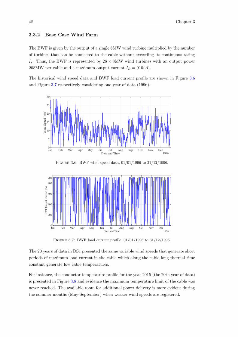
48 Chapter 3
3.3.2 Base Case Wind Farm
The BWF is given by the output of a single 8MW wind turbine multiplied by the number
of turbines that can be connected to the cable without exceeding its continuous rating
Is. Thus, the BWF is represented by 26 × 8MW wind turbines with an output power
208MW per cable and a maximum output current IB = 910(A).
The historical wind speed data and BWF load current profile are shown in Figure 3.6
and Figure 3.7 respectively considering one year of data (1996).
Jan Feb Mar Apr May Jun Jul Aug Sep Oct Nov Dec
Date and Time 1996
0
5
10
15
20
25
30
Win
d S
pee
d (
m/s
)
Figure 3.6: BWF wind speed data, 01/01/1996 to 31/12/1996.
Jan Feb Mar Apr May Jun Jul Aug Sep Oct Nov Dec
Date and Time 1996
0
200
400
600
800
900
BW
F O
utp
ut
Curr
ent
(A)
Figure 3.7: BWF load current profile, 01/01/1996 to 31/12/1996.
The 20 years of data in DS1 presented the same variable wind speeds that generate short
periods of maximum load current in the cable which along the cable long thermal time
constant generate low cable temperatures.
For instance, the conductor temperature profile for the year 2015 (the 20th year of data)
is presented in Figure 3.8 and evidence the maximum temperature limit of the cable was
never reached. The available room for additional power delivery is more evident during
the summer months (May-September) when weaker wind speeds are registered.

Probabilistic Thermal Risk Estimation Methodology 49
Jan Feb Mar Apr May Jun Jul Aug Sep Oct Nov Dec
Date and Time 2015
10
20
30
40
50
60
70
80
90
Tem
per
atu
re (°C
)
Figure 3.8: BWF Conductor temperature profile, 01/01/1996 to 31/12/1996.
3.3.3 Hypothetical Overplanting Scenarios
Hypothetical wind farm overplanting cases are defined to induce cable temperature ex-
ceedances in the system. The export cable system studied is deliberately overloaded
with a load current higher than the continuous rating Is by the addition of a greater
number of wind turbines compared to the BWF=26 wind turbines.
The cable overload cases studied in this chapter are WFO1=28 wind turbines; WFO2=29
wind turbines; and WFO3=30 wind turbines. The percentage of cable rating increment
compared to the static rating of the cable Is, as well as the wind farm overplanting
factor and maximum load current output Imax, are presented in Table 3.5.
WFO Overplanting RatingImax
Case Factor Increment
BWF n/a n/a IB = 910 (A)
WFO1 1.06 6% 980 (A)
WFO2 1.09 9.9% 1015 (A)
WFO3 1.13 13% 1050 (A)
Table 3.5: Hypothetical WFO cases
3.3.4 Example Wind Farm Assumptions
The load current time-series data from the explanatory wind farm presented above
generates the gross energy production which is the output energy obtained considering
a free stream of wind speed distribution at hub height for each one of the turbines [107].

50 Chapter 3
For instance, the main sources of energy losses in wind farm such as wake effects, wind
turbine availability and electric losses are neglected assuming an ideal experimental
scenario which for the case of wind farm overplanting studies generates an embedded
margin of conservatism in the results.
3.3.4.1 Wake Effect Losses
Wake effects losses in the turbine array are given by the reduction of wind speed down-
stream due to the impact of the airflow from a wind turbine on the surrounding turbines.
The wake effects from neighbouring wind turbines were neglected in the proposed ex-
ample even though in reality power losses due to wake effect range between 5% to 15%
in the case of an offshore wind farm [108].
An optimised spacing between wind turbines for reduced energy losses from the wind
park effect is assumed as suggested in [109]. Nevertheless, if required by the analysis, a
reductive factor for the inclusion of wake losses could easily be added to the load current
profile data once the details of wake losses for the particular offshore site studied are
known.
3.3.4.2 Wind Turbine Availability
During the lifetime of the project turbines availability is reduced by scheduled main-
tenance and repairs affecting the gross energy production. Thus, a percentage factor
accounting for turbine availability must be defined according to the case studied.
A figure of 96% wind turbine availability would represent a reasonable assumption ac-
cording to the study by DONG Energy in [110] however, the same study evidence that
for the case of offshore locations the data on wind turbines availability present variation
for different wind farms and year to year data. Thus, a reduction factor according to
the user’s needs can be added to the results to account for the losses according to the
specific study case.
3.3.4.3 Electrical Transmission Losses
The transmission of electric power from the wind turbines to the grid suffer electric losses
in the array cables, the offshore substation, the export cable and onshore substation
due to electrical inefficiency which generates a reduction of the calculated gross power
generated by the wind farm while also increasing the cable temperature due to Joule
losses in the cable.
A rough figure of the percentage of losses in the components mentioned above are:
Interarray cables 1-2% depending on cable size, length, voltage and lying topology;
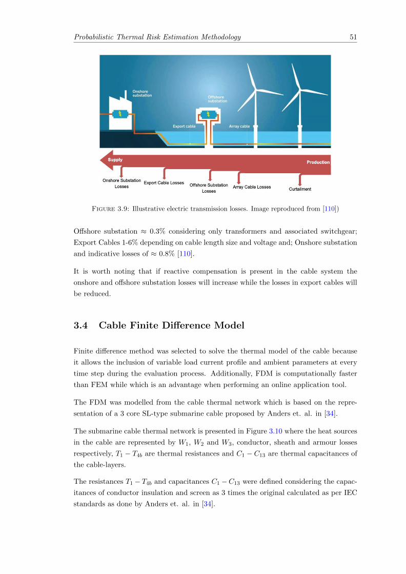
Probabilistic Thermal Risk Estimation Methodology 51
Figure 3.9: Illustrative electric transmission losses. Image reproduced from [110])
Offshore substation ≈ 0.3% considering only transformers and associated switchgear;
Export Cables 1-6% depending on cable length size and voltage and; Onshore substation
and indicative losses of ≈ 0.8% [110].
It is worth noting that if reactive compensation is present in the cable system the
onshore and offshore substation losses will increase while the losses in export cables will
be reduced.
3.4 Cable Finite Difference Model
Finite difference method was selected to solve the thermal model of the cable because
it allows the inclusion of variable load current profile and ambient parameters at every
time step during the evaluation process. Additionally, FDM is computationally faster
than FEM while which is an advantage when performing an online application tool.
The FDM was modelled from the cable thermal network which is based on the repre-
sentation of a 3 core SL-type submarine cable proposed by Anders et. al. in [34].
The submarine cable thermal network is presented in Figure 3.10 where the heat sources
in the cable are represented by W1, W2 and W3, conductor, sheath and armour losses
respectively, T1 − T4b are thermal resistances and C1 − C13 are thermal capacitances of
the cable-layers.
The resistances T1 − T4b and capacitances C1 −C13 were defined considering the capac-
itances of conductor insulation and screen as 3 times the original calculated as per IEC
standards as done by Anders et. al. in [34].

52 Chapter 3
T1 T2a T2b T3 T4a T4b
W1 C1 C2 C3 W2 C4 C5 C6 C7 C8 C9 W3 C10 C11 C12
o
C13
oθc θs θj θa θo θe θamb
o
Figure 3.10: Cable Thermoelectric Equivalent Circuit.
C1 = 3 ∗Qc;
C2 = 3 ∗ pQi;
C3 = 3 ∗ (1− p)Qi;
C4 = 3 ∗Qs;
C5 = 3 ∗ p′Qj ;
C6 = 3 ∗ (1− p′)Qj ;
C7 = Qf ;
C8 = p′′Qb;
C9 = (1− p′′)Qb;
C10 = Qa;
C11 = p′′′Qo;
C12 = (1− p′′′)Qo;
C13 = Qsoil;
T1 =Ti3
;
T2a =Tj3
;
T2b = Tb;
T3 = To;
T4a = Tamb1;
T4b = Tamb2;
W1 = 3Wc;
W2 = 3Ws;
W3 = Wa,
where the subscripts c, i, s, j, f , b, a, o and e correspond to conductor, insulation,
sheath, jacket, filler, bedding, armour, outer covering and external environment while p,
p′, p′′ and p′′′ are the Van Wormer coefficients for insulation, jacket, bedding and serving
are defined as per IEC 60287 [6].
The representation of the thermal resistance of ambient temperature must be split in at
least two thermal zones to account for situations when drying out of the soil or moisture
migration may occur [111]. In this thesis the calculation of T4 is therefore represented
by T4a and T4b considering the first thermal zone as half of the burial depth L and
following the calculation of T4b as an additional thermal layer over cable outer cover and
T4b calculated as the thermal resistance of thermal environment as follows:
T4a =1
(2 ∗ π)∗ ρsoil ∗ log
(1 +
(0.5 ∗ Ld10
));
T4b =1
(2 ∗ π)∗ ρsoil ∗ log
(u+
(√u2 − 1
));
u =
(2 ∗ L
d10 + 0.5 ∗ L
);
where u is a parameter to calculate the thermal resistance of thermal environment given
by IEC 60287 [6], ρsoil is the thermal resistivity of the soil, and d10 is the external
diameter of the outer serving.

Probabilistic Thermal Risk Estimation Methodology 53
The differential equations of the circuit for the calculation of temperatures at nodes θc,
φs, θj , θa, θo, θe are obtained and approximated using the backward finite difference
approach as in [35]
d
dtθm =
θm(t)− θm(t− 1)
∆t(3.3)
where m is substituted by the subscripts c, i, s, j, f , b, a, o and e accordingly. The
obtained system of linear equations A ∗ x = B is solved for x at each time step to
obtain the temperatures at each node of the cable considering changes in load data.
The finite-difference model equations of the cable system can be found in Appendix A.
3.5 Proposed Thermal Risk Estimation Methodology
The algorithm proposed for the hours ahead TRE can be described in three main steps:
• Estimation of future load generation using the MCS methods;
• Calculation of conductor temperature considering the sampled data;
• Hours ahead thermal risk estimation considering likely cable temperatures.
The flow diagram in Figure 3.11 presents an overview of the developed methodology. The
cable FDM calculates the conductor temperature at every 1 hour time step, considering
actual load current in the cable system. The consideration of a one hour time step was
given by the sampling time in the data set however it can be modified as necessary. On
the other hand, shorter time steps i.e 30 min or 10 min induce an increment in computer
calculations and thus longer computational times.
The dashed rectangle in Figure 3.11 represents a parallel subroutine of the main FDM
calculation. The three main steps in the dashed rectangle are 1) the generation of random
load samples via MCS; 2) the estimation of the likely cable conductor temperatures via
FDMsub and; 3) the evaluation of thermal risk hours ahead.
3.5.1 Training and Testing Datasets
The time-series load current profiles for each WFO case is divided into training and
testing. The testing year is defined as the last year of DS1 (year 2015) while three
lengths of training set (Ts) were defined as per Table 3.6 along the studied time ahead
windows for thermal risk estimation selected as h = 6, 12, 24. hours. Longer hours ahead
estimation periods were tested i.e. 36 and 48 hours however the longer the estimation
period the greater the estimations errors.

54 Chapter 3
FDMmain
Load current,soil parameters,
burial depth
Timeseries
load data
Real time Tr
Start
Identify Month
MonthlyPDFs
1) Generate ran-dom load samples
2) Evaluateload scenar-ios: FDMsub
3) ThermalRisk evaluation
is there riskof Te > 90Cin the next h
hours?
Action Required
Not ActionRequired
t = t+ 1
no
yes
Figure 3.11: Probabilistic Methodology, flowchart.
The data set used was 20 years long thus 5, 10 and 19 years long training sets were
tested to investigate if larger datasets could improve the estimation accuracy. The
shortest training set was defined considering the length of the survey data gathered at
the beginning of the offshore project.
Training Set Length in years Date period
Ts 1 5 01/01/1996− 31/12/2000
Ts 2 10 01/01/1996− 31/12/2005
Ts 3 19 01/01/1996− 31/12/2014
Table 3.6: Training data sets
3.5.2 Probabilistic Load Current Generation
The estimation of future load in the cable is generated by an MCS from the PDF of the
month in which the analysis is performed. The load current sampling process generates

Probabilistic Thermal Risk Estimation Methodology 55
a matrix S containing n× h series of load current values such that
S(n×h) =
x1,1 . . . x1,h
.... . .
...
xn,1 . . . xn,h
(3.4)
where h is the hours ahead horizon selected h = 6, 12, 24, and n is the number of
iterations in the MCS.
3.5.3 Probabilistic Conductor Temperature Calculation
The matrix of conductor temperatures Te is generated considering the evaluation of the
load values in S at every time step (t) by the FDMsub. The temperature evaluation
in FDMsub considers as initial condition the real-time load current I(t)and conductor
temperature Tr(t) calculated by the FDMmain such that
Te(n×h) =
y1,1 . . . y1,h
.... . .
...
yn,1 . . . yn,h
. (3.5)
The number of iterations n in the MCS was set to 10, 000 which was enough to represent
the distribution of the data in the sampled probability distribution according to the
original population data. The alternative approach is to calculate the confidence level
from the sampled data according to the desired precision. For example, in a normally
distributed sample a 95% confidence interval will lie in the range of ± 2 σ where σ is
the standard deviation form the original data PDF [112].
3.5.4 Probabilistic Thermal Risk Estimation
The conductor temperatures in Te are analysed to calculate the likely risk of cable
overheating in the following hours (r). The thermal risk r is calculated based on the
number of cases where the conductor temperatures in Te exceeds the cable temperature
limit Tlimit = 90C. The risk of cable overheating is thus given by the equation
r(Te > Tlimit) =b
N. (3.6)
where N is the total number of sampled values in the MCS and b the number of tem-
perature incidences above Tlimit.

56 Chapter 3
Thus, at every time step (t) in main routine FDMmain the subroutine performs the
Monte Carlo Simulation process, conductor temperature calculations using FDMsub and
estimates the h hours ahead of likely thermal risk r.
3.5.5 Methodology Evaluation Process
In order to evaluate the accuracy of the methodology a comparison of the estimated
thermal risk r against the realistic risk r was carried out. The realistic risk r was
calculated considering the realistic conductor temperatures Tr(1×h) = yr(t + 1), yr(t +
2), . . . , yr(t+ h) from time (t+ 1) to (t+ h) when they become available in FDMmain.
Thus, the realistic risk r is defined as follows
r(Tr > Tmax) =brh. (3.7)
where, similarly to equation 3.6, h is the total number of values and br the number of
temperature incidences above Tlimit.
3.5.5.1 Accuracy of the Thermal Risk Estimations
The thermal risk estimations r and realistic risk r are given in a [1 − 0] value where
1 = 100% risk h hours ahead. One year of testing produces g thermal risk calculations
which are then compared and evaluated considering the mean absolute error (MAE)
MAE =1
g
g∑t=1
| r(t)− r(t) | (3.8)
and root mean squared error (RMSE)
RMSE =
√√√√1
g
g∑t=1
(r(t)− r(t))2. (3.9)
Both measurements represent the average prediction error in the same units as the
variable analysed, and are negative oriented, thus, the lower values obtained represent
more accurate estimation results. MAE is affected in direct proportion by the absolute
value of error, while, RMSE square the errors before calculating their mean which gives
more weight to large but infrequent errors. Thus, calculating both measures gives an
idea of the average accuracy of the methodology while accounting for the frequency of
large errors in the estimation.

Probabilistic Thermal Risk Estimation Methodology 57
3.5.5.2 Accuracy of the Methodology to Estimate Risk Ahead
The accuracy of the methodology to estimate risk h hours ahead was calculated using
a binary classification approach where the estimated risk r and realistic risk r for the
testing year are evaluated as in Table 3.7.
r > 0 r = 0
r > 0True Positive False Positive
(TP) (FP)
r = 0False Negative True Negative
(FN) (TN)
Table 3.7: Binary Classification of TRE
The percentage of True Positive cases is when r and r were both non zero; True Negative,
indicates the percentage of cases where r and r were both zero; False Negative, is the
percentage of cases where the TRE algorithm did not estimate the realistic thermal
overheating experienced by the cable and; False Positive, represents the percentage of
cases where the methodology estimated a thermal risk but no real thermal overheating
was experienced by the cable.
Finally, the categories TP and TN are considered successful thermal risk estimations
while categories FP and FN are considered unsuccessful estimations or misclassifications.
3.6 Methodology Testing Results
The computational algorithm was developed using MatLab software in a MacBook Pro
with a 2.2 GHz Intel Core i7 processor, no special requirements are needed. The method-
ology was tested considering 6, 12 and 24 hours ahead windows, three WFO cases and
TS lengths as per Tables 3.5 and 3.6.
The probabilistic TRE algorithm was tested over one year of data thus 8760 estimations
were obtained, stored and evaluated as explained in section 3.5.5. The probabilistic
subroutine took approximately 3.9 seconds to perform an estimation (steps in the dashed
box in Figure 3.11) and continue to update the next time step in the main FDM routine,
thus, one year of testing for every case considered took in average 3500 seconds. It is
worth noting that the code has not been optimised for speed thus it could be faster if
transported to another programming language.

58 Chapter 3
3.6.1 Accuracy of the Methodology to Estimate Thermal Risk
The percentages of successful (TP and TN) and unsuccessful (FP and FN) cable thermal
risk estimations in Tables 3.8, 3.9 and 3.10 presents the accuracy of the probabilistic
methodology to detect thermal risk according to the binary classification in Table 3.7.
6 hours ahead TRE
RatingCategory
Ts1 Ts2 Ts3
Increment % % %
6%
TN 87.28 87.5 87.39
TP 11.65 11.2 11.43
FN 0.365 0.81 0.58
FP 0.696 0.47 0.59
(TN+TP) 98.93 98.7 98.82
(FP+FN) 1.06 1.29 1.17
9.9%
TN 74.76 75.58 75.18
TP 21.87 21.59 21.75
FN 0.628 0.9 0.74
FP 2.729 1.91 2.31
(TN+TP) 96.64 97.17 96.93
(FP+FN) 3.35 2.82 3.06
13.7%
TN 62.14 62.18 61.56
TP 31.29 31.49 31.58
FN 0.799 0.6 0.51
FP 5.756 5.72 6.33
(TN+TP) 93.44 93.67 93.14
(FP+FN) 6.55 6.32 6.85
Table 3.8: Results of thermal risk estimation considering 6h ahead TRE.
From the results in tables 3.8 to 3.10 it can be seen that the overall performance of
the methodology to estimate thermal risk is not highly affected by the amount of data
used for the construction of the monthly PDF. This characteristic, is an advantage for
the application of the methodology, considering that, the environmental data collected
in early stages of offshore wind projects (usually 3 to 5 years of data) can be sufficient
to run the analysis. Given that, the overall results in tables 3.8 to 3.10 do not reflect
outstanding improvement when considering Ts2 and Ts3, the results given by shortest
training set Ts1 are analysed in detail.
The comparison of tables 3.8, tables 3.10 and tables 3.10 for Ts1 reveals that the number
of successful risk estimations (TN +TP) is increased when the hours ahead estimation
period is decreased. For instance for the 6% cable overload percentage the results from
the 24, 12 and 6 hours ahead horizons are 96.33%, 97.64% and 98.93% respectively
while the percentages of unsuccessful risk estimations (FN+FP) were 3.66%, 2.35% and
1.06%.

Probabilistic Thermal Risk Estimation Methodology 59
12 hours ahead TRE
RatingCategory
Ts1 Ts2 Ts3
Increment % % %
6%
TN 85.33 86.33 85.77
TP 12.31 11.32 11.84
FN 0.96 1.94 1.42
FP 1.39 0.4 0.96
(TN+TP) 97.64 97.65 97.61
(FP+FN) 2.35 2.34 2.38
9.9%
TN 69.57 71.39 70.01
TP 23.23 22.44 23.0
FN 1.87 2.66 2.10
FP 5.31 3.49 4.86
(TN+TP) 92.81 93.83 93.02
(FP+FN) 7.18 6.16 6.97
13.7%
TN 51.84 51.66 51.08
TP 34.01 34.51 34.54
FN 1.63 1.13 1.10
FP 12.50 12.68 13.27
(TN+TP) 85.86 86.18 85.62
(FP+FN) 14.13 13.81 14.37
Table 3.9: Results of thermal risk estimation considering 12h ahead TRE.
Naturally higher overloads in the cable induce more chances of the cable being over-
heated and leads to a greater chance of misclassifications (FN+FP). As an example,
in the 24 ahead estimation (table 3.10) the 6% overload case presents 3.66% of unsuc-
cessful estimations while the 13.7% overload case presents 13.14%. The severity of the
misclassification results is analysed separately in the following section.
Remark 1:Comparing the percentage results for the same hours ahead period consid-
ering the 3 WFO cases (table 3.8) it is evident by the increment of TP cases that the
methodology can estimate thermal risk. However, the increment of category FP also im-
plies that the amount of cases that the algorithm predicts a non existent risk is increased
as well.
The underlying reason is that the MCS procedure does not consider the initial load in the
cable when generating the load current matrix S, furthermore, the individual samples
are also independent of one to another. In other words, the values in the sampled series S
does not present dependency which induces greater un-realistic estimations of calculated
cable temperatures. The load sampling dependency problem generation is addressed in
Chapter 4.

60 Chapter 3
24 hours ahead TRE
RatingCategory
Ts1 Ts2 Ts3
Increment % % %
6%
TN 83.28 84.35 83.55
TP 13.04 11.52 12.59
FN 2.27 3.79 2.73
FP 1.38 0.32 1.12
(TN+TP) 96.33 95.88 96.12
(FP+FN) 3.66 4.12 3.85
9.9%
TN 66.11 67.34 66.28
TP 25.24 24.01 24.92
FN 3.71 4.95 4.04
FP 4.92 3.68 4.74
(TN+TP) 91.35 91.35 91.21
(FP+FN) 8.64 8.64 8.79
13.7%
TN 49.21 48.20 48.51
TP 37.65 38.62 38.67
FN 3.25 2.26 2.22
FP 9.88 10.89 10.58
(TN+TP) 86.86 86.83 87.19
(FP+FN) 13.14 13.16 12.80
Table 3.10: Results of thermal risk estimation considering 24h ahead TRE.
3.6.2 Estimated Risk Error
The error between the estimated risk (r) and real risk (r) were calculated as described
in section 3.5.5 and the calculated RMSE and MAE are presented in Table 3.11. The
table summarises the results of the simulations performed considering Ts1 for the three
overload cases and time horizons ahead.
The most accurate estimations in both measurements are given by the 6 hours ahead
estimations with MAE’s between 0.096 and 0.209 and RMSE between 0.288 and 0.386
depending on the overload cases. It can be seen that the highest mean average error
is 0.257 corresponding to the 13.7% current overload 24 hours ahead. The same case
present the highest root mean squared error equals to 0.444. The work presented in
chapter 5 will look at the reduction of these error measurements.
3.6.3 Severity Analysis of Misclassifications Incidents
A closer analysis to the misclassification categories FN and FP in the results consid-
ering Ts1 in Table 3.8, Table 3.9 and Table 3.10 was carried out in order to understand
the severity of the temperature exceedance involved.

Probabilistic Thermal Risk Estimation Methodology 61
Ts1
Rating 6 hours 12 hours 24 hours
Increment MAE RMSE MAE RMSE MAE RMSE
6% 0.096 0.288 0.101 0.296 0.103 0.292
9.9% 0.167 0.365 0.181 0.387 0.188 0.388
13.7% 0.209 0.386 0.240 0.430 0.257 0.444
Table 3.11: Accuracy of thermal risk estimations [0 to 1], data set 1
The real cable temperature Tr and the estimated temperature values Te at each of
the times when misclassifications occurred were extracted from the simulated data and
evaluated. In the case of FN incidents, two severity subcategories were defined as
FNs1=(90C < Tr < 92C) and FNs2=(Tr > 92C). In the case of category FP, the
real cable temperature was not at risk but, the estimated temperatures are extracted to
evaluate the range of inaccuracy of the methodology.
Figure 3.12 considers only the obtained FN percentages for each WFO case and time
ahead window for the case of Ts1 considering the severity subcategories FNs1 and FNs2.
The percentages of FN cases falling in subcategory FNs1 is always higher than 50% even
for the most higher overload percentage (WFO3) and larger time window ahead (24
hours).
!"#$%
&'%
!"()%
&)"')%
#)"&*%
$"&*%
+("*,%
#,"),%
)''%
,#"!#%
*'%
,#"&,%
(*",,%
!*"(&%
,+"(&%
$&"))%
!'"*)%
'% )'% &'% +'% #'% !'% $'% ('% *'% ,'% )''%
$-./-0/12.345)
$-./-0/12.345&
$-./-0/12.345+
)&-./-0/12.345)
)&-./-0/12.345&
)&-./-0/12.345+
&#-./-0/12.345)
&#-./-0/12.345&
&#-./-0/12.345+
467).8,'! 9.:;.<.,&!= 467&.8:;.9.,&!=
Figure 3.12: Analysis of misclassification cases FN according to severity, Ts1
As mention previously in section 2.1.2, the thermal ageing is not an instantaneous process
but a gradual deterioration of the material properties when operated over its maximum
temperature limit. The same applies to the different ageing factors that affect the cable
which are thermal, electrical, mechanical and environmental ageing mechanisms that
can cause irreversible changes in XLPE insulations.

62 Chapter 3
Some examples of the above factors are high or low-temperature cycles, voltage impulses,
current overloads, tensile fatigue, bending, vibration, humidity and radiation [113]. In
the worst-case scenario, the effects of these ageing mechanism affecting the cable fre-
quently over longe times can generate hardening, softening, loss of mechanical strength,
swelling, conductor penetration, rotation of cable movement of joints and terminations
and mechanical rupture.
Assuming the cable has not been aggressively damaged by the above ageing factors
a temperature exceedance of +2C above the maximum operating temperature of the
insulation would not generate an major problem. Furthermore, the XLPE emergency
temperature conditions is 130C.
The analysis of the false-positive cases (FP) for the case of Ts1 is presented in Table
3.12 from the estimated vs real cable temperature to understand the severity of the
misleading estimations which cause of the methodology estimating a non-existing risk.
For instance, the real conductor temperature at points where the methodology estimates
a non-existing risk is seen to vary between 36C to 89C while the real estimated values
are over 90C.
It is important to clarify that the purpose of the methodology was focused on thermal
risk estimation, not on temperature estimation. For instance, the reason for the dif-
ference between the real and estimated temperatures is thought to happen when that
methodology does not quickly follow the swings down in the load current generation be-
cause the MCS does not takes into account the instantaneous load current in the cable
as mention in remark 1.
Remark 2:The more severe misclassifications category is FP because the misleading
estimated temperatures in this category can lead to unnecessary power curtailment when
in reality the cable is not in danger. Chapter 4 investigates this problem further and
identifies ways in which better prediction performance can be achieved.
3.6.4 Conductor Temperature and Risk Estimation
The estimated cable temperatures generated every hour are the estimated likely range
of temperatures that the cable can experience in the next hours. The ability of the
methodology to derive a 6 hour ahead thermal risk estimation evidenced by Figures
3.13 and 3.14.
The figures present the BWF conductor temperature and the realistic cable temperature
given by WFO3 during a period of June 17-July 07 where no thermal risk was present
nor estimated by the methodology, see Figure 3.13.

Probabilistic Thermal Risk Estimation Methodology 63
Ts1
WFOTotal FP
6 hours ahead
Tr Te% Min Max Min Max
1 0.696 71.8C 89.98C 90C 93.99C
2 2.729 59.45C 89.99C 90.01C 97.48C
3 5.756 48.93C 89.99C 90C 101.72C
WFOTotal FP
12 hours ahead
Tr Te% Min Max Min Max
1 1.39 49.48C 89.93C 90C 94.02C
2 5.31 41.33C 89.99C 90C 98.01C
3 12.5 36.65C 89.99C 90.01C 103.49C
WFO Total FP24 hours ahead
Tr Te% Min Max Min Max
1 1.38 42.72C 89.91C 90.01C 93.3C
2 4.92 38.3C 89.97C 90C 97.54C
3 9.88 38.26C 89.99C 90.01C 103.1C
Table 3.12: Analysis of misclassification cases FP, Ts1
A different period from March 25- April 15 is presented in Figure 3.14 for which WFO3
generates and overheating in the cable as also estimated by the methodology. For in-
stance, the times at which the algorithm estimates thermal risk 6h ahead is indicated
by (*) in figure 3.14.
Jun 19 Jun 22 Jun 25 Jun 28 Jul 01 Jul 04 Jul 07
Date and Time 2015
20
30
40
50
60
70
80
90
Co
nd
uct
or
Tem
per
atu
re (
ºC)
WFO3
BWF
Figure 3.13: Estimated Conductor Temperature Ranges, 13% overload
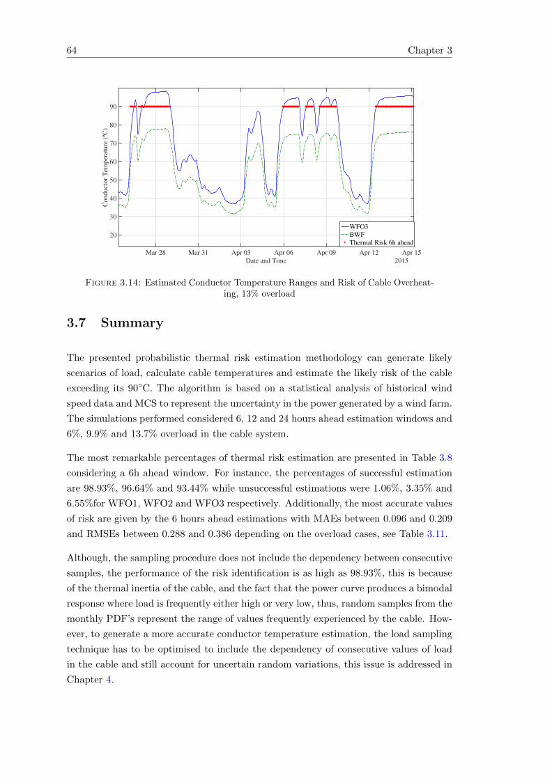
64 Chapter 3
Mar 28 Mar 31 Apr 03 Apr 06 Apr 09 Apr 12 Apr 15
Date and Time 2015
20
30
40
50
60
70
80
90C
on
du
cto
r T
emp
erat
ure
(ºC
)
WFO3
BWF
Thermal Risk 6h ahead
Figure 3.14: Estimated Conductor Temperature Ranges and Risk of Cable Overheat-ing, 13% overload
3.7 Summary
The presented probabilistic thermal risk estimation methodology can generate likely
scenarios of load, calculate cable temperatures and estimate the likely risk of the cable
exceeding its 90C. The algorithm is based on a statistical analysis of historical wind
speed data and MCS to represent the uncertainty in the power generated by a wind farm.
The simulations performed considered 6, 12 and 24 hours ahead estimation windows and
6%, 9.9% and 13.7% overload in the cable system.
The most remarkable percentages of thermal risk estimation are presented in Table 3.8
considering a 6h ahead window. For instance, the percentages of successful estimation
are 98.93%, 96.64% and 93.44% while unsuccessful estimations were 1.06%, 3.35% and
6.55%for WFO1, WFO2 and WFO3 respectively. Additionally, the most accurate values
of risk are given by the 6 hours ahead estimations with MAEs between 0.096 and 0.209
and RMSEs between 0.288 and 0.386 depending on the overload cases, see Table 3.11.
Although, the sampling procedure does not include the dependency between consecutive
samples, the performance of the risk identification is as high as 98.93%, this is because
of the thermal inertia of the cable, and the fact that the power curve produces a bimodal
response where load is frequently either high or very low, thus, random samples from the
monthly PDF’s represent the range of values frequently experienced by the cable. How-
ever, to generate a more accurate conductor temperature estimation, the load sampling
technique has to be optimised to include the dependency of consecutive values of load
in the cable and still account for uncertain random variations, this issue is addressed in
Chapter 4.

Probabilistic Thermal Risk Estimation Methodology 65
The proposed algorithm can help the system operators to optimise the amount of power
that can be transferred from offshore installations. A 6h ahead estimation of thermal
risk allows sufficient time to apply a curtailment strategy i.e. reduce generation output if
a risk of cable overheating is detected. On the other hand, in the cases where the power
output in the system has been high for a certain time and the temperature of the cable
is over 85C the system operator could rely on the probabilistic analysis estimating no
risk, given comparable experiences in the historical data.
The proposed methodology is well suited as an offline simulation tool in the design
phase of wind farm projects in order to evaluate the reduction in export cable size.
Additionally, the results show that the methodology can generate accurate thermal risk
estimations with just 5 years of historical data that can be collected from initial surveys
in an offshore wind farm location which is an important characteristic given that the
availability of data from an offshore location is limited.
A conference paper containing the methodology and results presented in this chapter
was written, published and presented in the international conference on Probabilistic
Methods Applied to Power Systems (PMAPS 2018) in Boise, Idaho in the United States
in June 2018 [114].


Chapter 4
Markov Based Thermal Risk
Estimation for Offshore Export
Cables
The results obtained in Chapter 4 evidenced that the MCS based methodology was able
to estimate thermal risk however the algorithm load current sampling process did not
consider the actual load current when sampling future load scenarios thus generating
highly variable series of load current. Even though the overall MCS was able to esti-
mate risk because the sampled load was tested considering actual cable temperature, a
correction in the load current sampling would help to generate more realistic scenarios.
This chapter investigates the use of Markov Theory combined with the MCS process
to generate better load current predictions and improve the performance of the TRE
methodology in Chapter 3. The proposed methodology is a non-parametric analysis of
historical data based on MC models to predict probable load current states, from which
a MCS generates a series of likely load current scenarios that the cable could experience
in the following hours.
The study features the analysis of 1st and 3rd order Markov models considering the 3
WFO cases presented in Chapter 3 considering only the use of Ts1 (5 years of training
data) and a 6h ahead estimation window. The first and third-order TPM will be referred
to as MC1 and MC3 along the rest of this thesis.
The finite difference model of the cable previously presented is also used in this analysis
to solve the thermoelectric equivalent network of the cable and calculate the temperature
in real-time, while a subroutine of the FDM calculates the cable temperatures given the
MCS scenarios and the actual cable temperatures.
67
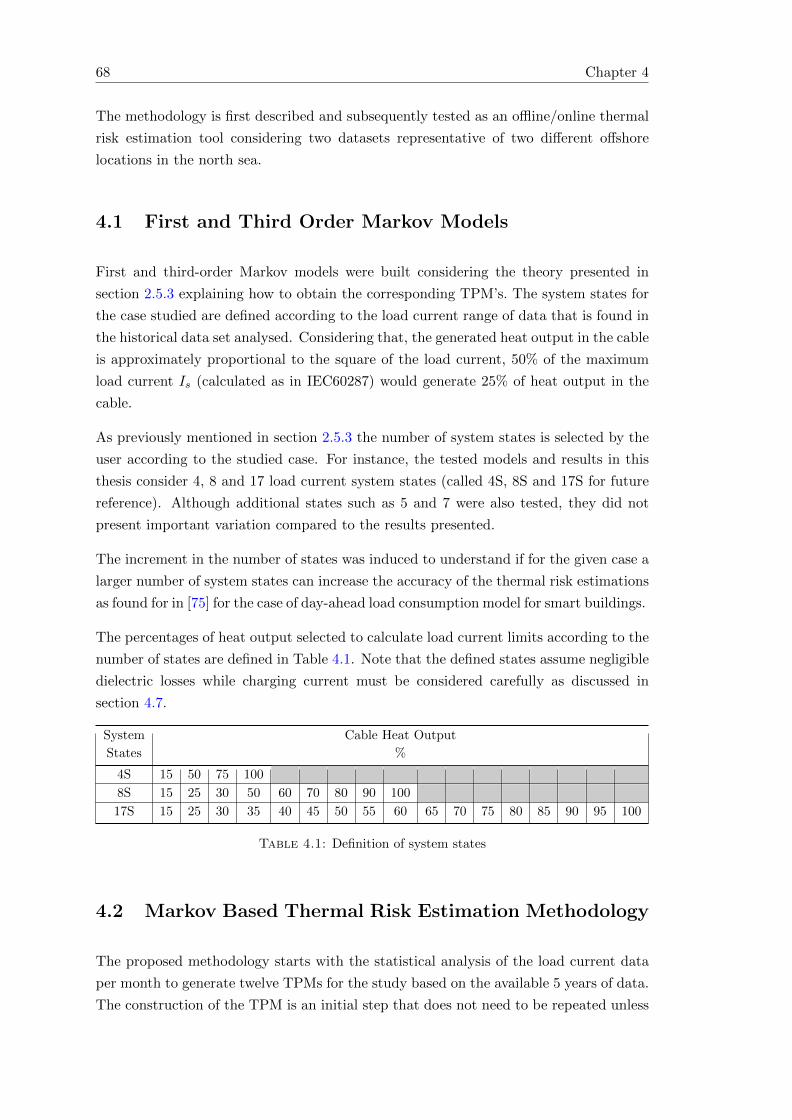
68 Chapter 4
The methodology is first described and subsequently tested as an offline/online thermal
risk estimation tool considering two datasets representative of two different offshore
locations in the north sea.
4.1 First and Third Order Markov Models
First and third-order Markov models were built considering the theory presented in
section 2.5.3 explaining how to obtain the corresponding TPM’s. The system states for
the case studied are defined according to the load current range of data that is found in
the historical data set analysed. Considering that, the generated heat output in the cable
is approximately proportional to the square of the load current, 50% of the maximum
load current Is (calculated as in IEC60287) would generate 25% of heat output in the
cable.
As previously mentioned in section 2.5.3 the number of system states is selected by the
user according to the studied case. For instance, the tested models and results in this
thesis consider 4, 8 and 17 load current system states (called 4S, 8S and 17S for future
reference). Although additional states such as 5 and 7 were also tested, they did not
present important variation compared to the results presented.
The increment in the number of states was induced to understand if for the given case a
larger number of system states can increase the accuracy of the thermal risk estimations
as found for in [75] for the case of day-ahead load consumption model for smart buildings.
The percentages of heat output selected to calculate load current limits according to the
number of states are defined in Table 4.1. Note that the defined states assume negligible
dielectric losses while charging current must be considered carefully as discussed in
section 4.7.
System Cable Heat Output
States %
4S 15 50 75 100
8S 15 25 30 50 60 70 80 90 100
17S 15 25 30 35 40 45 50 55 60 65 70 75 80 85 90 95 100
Table 4.1: Definition of system states
4.2 Markov Based Thermal Risk Estimation Methodology
The proposed methodology starts with the statistical analysis of the load current data
per month to generate twelve TPMs for the study based on the available 5 years of data.
The construction of the TPM is an initial step that does not need to be repeated unless

Markov Based Thermal Risk Estimation for Offshore Export Cables 69
the load current data is changed i.e studying a different WFO case, adding wind park
losses or charging losses to the data set. The next steps in the proposed algorithm are
explained below and represented by the diagram presented in Figure 5.2:
1. The first recurrent step in the methodology is the real-time calculation of conductor
temperature given the cable main FDM fdmmain described previously in chapter
3 and the instantaneous current I(t).
2. At every time step t in fdmmain (1 hour time steps) the cable temperature Tc(t)is calculated while a subroutine in the algorithm (red dotted line) performs a 6h
ahead estimation of load current state considering the actual load current I(t) and
the corresponding month TPM Phm where h = 6 and m = 1, 2, 3..., 12. Thus,
given the actual load current system state at time (t), the most likely load current
system state of the system at time t+ 6 is estimated.
3. Given the 6h ahead state estimation the MCS generates the scenario sampling from
the load current data in the forecasted system state to form matrix X containing
a series of values which are all within the same load current range, such that
X(n×h) =
x11 . . . x1h...
. . ....
xn1 . . . xnh
(4.1)
where n represents the number of iterations in the MCS and h = 6 represents the
number of steps ahead in the estimation.
Note: The sampled load current scenarios follow the direction of the actual load
direction i.e. If the difference between I(t)-I(t-1) is positive, the load current is
increasing thus, the random sampling follows the same incremental pattern for the
next 6h ahead estimation.
4. The sampled load current scenarios in X are then evaluated by the FDM subroutine
fdmsub considering the actual cable temperature Tc(t), as initial conditions for the
evaluation of the likely load current data. The calculated conductor temperatures
T ′c are used to form a probability distribution function PDFT ′c(t) of likely conductor
temperatures for the next 6h ahead.
5. Considering PDFT ′c(t) a likely thermal risk R′(t) is estimated as explained in sec-
tion 4.2.1.
6. The next step is the repetition of steps 1 to 5 considering I(t)=i(t+1). When
t = t + 6 in fdmmain the realistic risk R(t) is calculated as explained in Section
4.2.3.

70 Chapter 4
Start
Data Pre-processing:Given ws(m/s) calcu-late: I(t) = IWFO(t)
Statistical Analysis:Given I(t) calculate: Pm
fdmmain:Given I(t)
Calculate Tc(t)
NewData:I(t)
State Estimation:Given I(t), q = i,
and Phm
Calculate stateq = j for I(t + h)
Scenario Sampling:For state I(t + h) ∈q = j, MCS gen-
erates: X(n×h)
fdmsub:Given X(n×h)
and Tc(t) Cal-culate PDF T ′
c(t)
Risk Estimation:Given PDFT ′
c(t)
Calculate R′(t)
Risk Calculation:Given
Tc(t + 1, . . . , t + h)Calculate R(t)
Thermalrisk?
Curtailment:I(t) = IB(t + 1)
yes
I(t) = I(t + 1)
no
Figure 4.1: Offline (black) and online (black+blue) methodology, flowchart.
4.2.1 Forward Estimated Risk
The estimation of thermal risk R′ is calculated at each time step t considering the
probabilistic distribution of conductor temperature (PDFT ′c(t)) obtained from fdmsub.
The risk R′(t) is calculated by
R′(t) =T ′c (t+ 1, . . . , t+ h) ≥ Tlimit
h(4.2)
where T ′c (t + 1, . . . , t + h) ∈ PDFT ′c(t) represents the h most probable conductor tem-
peratures considering the central tendency values.
4.2.2 Realistic Thermal Risk
The realistic thermal risk R is calculated considering the conductor temperatures calcu-
lated by fdmmain. Given that R′(t) represents a likely thermal risk h hours ahead, the

Markov Based Thermal Risk Estimation for Offshore Export Cables 71
conductor temperatures Tc from time (t+ 1) to (t+h) are used to estimate the thermal
risk R(t) as
R(t) =Tc(t+ 1, . . . , t+ h) ≥ Tlimit
h(4.3)
which reflects the number of occasions on which the cable temperature exceeded Tlimit =
90C. R′(t) and R(t) are given in a [0 to 1] range where 1 = 100% thermal risk h hours
ahead.
4.2.3 Conductor Temperature Interval
Additionally, to the estimated risk R′(t) an interval of likely conductor temperatures
is derived at each time step from PDFT ′c(t). The central value of the interval, T ′c50(t),
is represented by the 50th percentile which is the value below which the 50% of the
observations in the sampled PDFT ′c(t) fall. The minimum and maximum values of the
interval are given by the 5th and 95th percentiles, T ′c5(t) and T ′c95(t) respectively.
4.3 Definition of Study Case
The studied cable system is the same as the study case presented in Chapter 4, see
section 3.3.1. Burial depth is kept constant for the section of the cable studied however,
this can be easily modified to study a different section of the cable such as a limiting
hot spot or multiple analysis of the cable at k different sections considering different soil
parameters i.e thermal conductivity, laying depth and ambient temperature.
Additionally, the BWF and three WFO cases defined in Chapter 4 section 3.3.2 and
3.3.3 respectively are used for the testing of the methodology in this chapter.
4.3.1 Load Current Datasets: DS1, DS2
The methodology proposed in this chapter is tested considering two data sets of hourly
sampled wind speed data, extrapolated from 50m to 110m over sea level. The testing of
two different sets is meant to test the algorithms ability to generate accurate estimations
considering only 5 years of data from the offshore locations studied.
DS1 previously defined in Chapter 4 while data set 2 (DS2) dated from 01/01/1979 to
31/12/2015 is representative of another offshore location in the North Sea also obtained
from MERRA analysis [105]. Table 4.2 presents the distribution of training and testing
years for both data sets.

72 Chapter 4
Data Set Length in Years Date Training Years Testing Year
DS1 20 01/01/1996 - 31/12/2015 01/01/1996 - 31/12/2000 01/01/2015 - 31/12/2015
DS2 36 01/01/1979 - 31/12/2015 01/01/1979 - 31/12/1983 01/01/2015 - 31/12/2015
Table 4.2: Training and testing years, DS1 and DS2.
4.4 Simulation and Evaluation Process
The computational algorithm and the simulations described below were developed using
MatLab software. The Markov Chain models analysed the first 5 years of DS1 and DS2
to obtain the TPM’s while the year 2015 was used for testing. The combination of 1st
and 3rd order TPM’s using 4, 8 and 17 states generated 6 MC models called 4S MC1,
4S MC3, 8S MC1, 8S MC3, 17S MC1, 17S MC3 through the rest of the Chapter.
The models were tested considering DS1 and a 6h ahead estimation window while DS2
was used to demonstrate that the methodology can be applied to different offshore
locations given its non-parametric nature.
4.4.1 Offline Thermal Risk Estimation
The offline simulation was described in steps 1 to 6 in section 4.2 and shown in black ink
in Figure 5.2. It consists of the calculation of hourly 6h ahead thermal risk estimations
and conductor temperatures for the given WFO case over the year of testing data without
further actions.
The estimated variables R′(t), T ′c50(t), T ′c5(t) and T ′c95(t) are stored at every time step
while the corresponding Tc(t + 6) and R(t) are calculated 6h into the future. The
variables are then used to calculate the accuracy of the methodology to estimate likely
thermal risk ahead.
The accuracy of the method to calculate thermal risk 6h ahead is first evaluated consid-
ering the binary classification presented in Chapter 4, Table 3.7 considering the nomen-
clature change in this chapter where the realistic thermal risk r is given by R(t) and
the estimated risk r is represented by R′(t). This approach reflects the actual success of
the methodology in estimating a thermal risk 6h ahead. Additionally, the error between
the estimated (R′) and realistic (R) thermal risk are evaluated considering the mean
absolute error (MAE) and root mean squared error (RMSE) as for the case of the purely
MCS based methodology in Chapter 4 considering equations 3.8 and 3.9. The consistent
evaluation process is performed with the objective of results comparison.

Markov Based Thermal Risk Estimation for Offshore Export Cables 73
4.4.2 Online Thermal Risk Estimation and Curtailment
The online simulation follows the same steps described for the offline simulation, however,
it also includes the steps in blue ink in Figure 5.2 which perform an automatic power
curtailment when the methodology estimates a likely thermal risk 6h ahead.
For instance, if any percentage of risk is estimated at time t a reduction in I(t + 1)
is applied. The reduction in current is equivalent to the curtailment of the additional
capacity installed according to the WFO case studied, in other words, the BWF rating
IB(t+1) is applied. On the other hand, if no thermal risk is estimated the original input
current I(t+ 1) for the WFO case is used.
The modified input current profile Inew(t) and corresponding conductor temperature
Tcnew(t) are then used to calculate the next 6h ahead thermal risk estimation R′new(t).
Given that the original data profiles are modified in real-time a new thermal risk Rnew
is calculated, while the risk estimation for the un-curtailed case (R) is also stored for
comparison.
The accuracy of the methodology to mitigate thermal risk is evaluated comparing the
realistic thermal risk R(t) which would be faced if no curtailment was applied and
the new real thermal risk Rnew(t) considering the curtailment performed online. The
comparison of risk before and after curtailment generates the categories described in
Table 4.3.
Classification Risk Before Risk After
Case Curtailment Curtailment
No Risk R(t) = 0 Rnew(t) = 0(NR)
Risk Mitigated R(t) > 0 Rnew(t) = 0(RM)
Risk Decreased R(t) > 0 0 < Rnew(t) < R(t)(RD)
Risk Increased R(t) > 0 Rnew(t) > R(t)(RI)
Risk Remained R(t) > 0 Rnew(t) = R(t)(RR)
Table 4.3: Online thermal risk evaluation.
The appearance of remaining risk classification cases RD, RI, RR is due to the conser-
vative approach of curtailment applied which is sustained for only one hour. The given
curtailment length can be increased to reduce/avoid the remaining risk after curtailment
categories.

74 Chapter 4
4.5 Methodology Testing Results
The results in this section correspond to the offline and online evaluation of the proposed
methodology considering MCM of 1st and 3rd order TPM’s using 4, 8 and 17 states,
abbreviated as 4S MC1, 4S MC3, 8S MC1, 8S MC3, 17S MC1, 17S MC3 through the
rest of the section. DS1 was used for the modelling and evaluation of all the MCM in
section 4.5.1 and 4.5.3 while DS2 is used in Section 4.5.4.
4.5.1 Offline Simulation Results: DS1
Figure 4.2 presents the results corresponding to the one-year evaluation of MAE and
RMSE errors betweenR′ andR. The most accurate predictions of thermal risk 6h ahead
are given by the 4S MC3 model with a MAE=0.0158 and RMSE=0.1057 for WFO1,
MAE=0.0417, and RMSE=0.1728 for WFO2 and, MAE=0.0419 and RMSE=0.1601 for
WFO3.
The results evidence that the increment in the number of defined states did not improve
the accuracy of the estimation results, due to level of uncertainty in the load current
generation profile. Conversely, the example in [16] presents a model for a day ahead
prediction of electrical consumption which did not present abrupt variations thus the
addition of additional system states increased the model accuracy.
On the other hand, the utilisation of 3rd order models generated better results for all
the cases compared to the 1st order models due to the consideration of not only one but
three past load current states as seen in [75] for the case of wind power forecasting.
0.0305 0.0304 0.0235 0.0221 0.0169 0.0158
0.1474 0.1468
0.1301 0.12560.1111 0.1057
0.0566 0.0538 0.0531 0.0483 0.0439 0.0419
0.2068 0.2007 0.19790.1875
0.1781 0.1728
0.0485 0.0424 0.04830.0362
0.0442 0.0417
0.17810.1626
0.1764
0.1475
0.16730.1601
8S_MC1 8S_MC3 17S_MC1 17S_MC3 4S_MC1 4S_MC3
Ris
k E
rror
[0-1
]
MC-Model
MAE_WFO1 RMSE_WFO1 MAE_WFO2
RMSE_WFO2 MAE_WFO3 RMSE_WFO3
Figure 4.2: Risk error calculated for the 6 MCM and 3 WFO cases.

Markov Based Thermal Risk Estimation for Offshore Export Cables 75
The errors between the realistic and estimated risk values presented in Figure 4.2 ev-
idence that MC3 models are more accurate than MC1 models. However, when the
number of states increases, so does the errors between R′ and R due to narrow state
limits which reduce uncertainty in the samples.
Additionally, it is also seen how a greater number of states does not necessarily reflect a
linear increment in the estimation of the error i.e. the models with 17 states were more
accurate than the models with 8 states while 4 states generate the best thermal risk
estimations.
The percentages of the thermal risk estimations generated by the methodology according
to the classification in Table 3.7 is presented in Figures 4.3, 4.4 and 4.5 corresponding
to the WFO1, WFO2 and WFO3 respectively testing the six MC models.
The most accurate model was chosen as the study case containing the highest percent-
age of successful identifications (TP+TN) and the smallest percentage of FN as this
case is potentially dangerous for the cable. For instance, the sum of percentages of
TP+TN represents successful estimations while FN+FP represents unsuccessful esti-
mations. Consistently with the results in Figure 4.2 higher accuracy is obtained with
4S MC3 model for the 3 WFO cases.
90.35 90.51 90.64 90.7 90.56 90.74
8.3
5
8.38
7.4
7.4
4
7.7
7.6
5
0.8
1
0.69
1.6
3
1.6
3
1.3
9
1.4
2
0.4
7
0.39
0.2
5
0.2
0.3
3
0.1
7
0
10
20
30
40
50
60
70
80
90
100
4S_MC1 4S_MC3 8S_MC1 8S_MC3 17S_MC1 17S_MC3
% E
stim
ated
Ris
k
MC-Model
True Negative True Positive False Negative False Positive
Figure 4.3: Percentage of positive and negative estimations, WFO1.
For the case of WFO1, in Figure 4.3, 98.90% of the thermal risk estimations correctly
identified a thermal risk 6h ahead while 1.10% were wrongly identified. As the over-
planting and load current increases, the chances of exceeding the temperature limit
also increase as seen for the cases WFO2 and WFO3 in Figures 4.4 and 4.5 where the
percentages of positive estimations (TP+TN) were 96.7% and 95.68% while FN+FP
were 3.28% and 4.32% for each figure respectively.

76 Chapter 4
76.11 76.46 76.59 76.95 76.31 76.9820.3
20.24
18.5
9
18.4
9
19.1
9
19.0
4
2.2
4
2.23
3.9
3.9
8
3.3
1
3.4
3
1.3
2
1.05
0.9
0.5
5
1.1
7
0.5
2
0
10
20
30
40
50
60
70
80
90
100
4S_MC1 4S_MC3 8S_MC1 8S_MC3 17S_MC1 17S_MC3
% E
stim
ated
Ris
k
MC-Model
True Negative True Positive False Negative False Positive
Figure 4.4: Percentage of positive and negative estimations, WFO2.
64.62 64.71 65.59 66.4 65.2 67.1
31.1
4
30.96
29.7
1
29.5
2
30.1
29.5
9
1 1.11
2.3
8
2.5
5
1.9
9
2.43.2
3
3.19
2.3
1.5 2.6
9
0.7
6
0
10
20
30
40
50
60
70
80
90
100
4S_MC1 4S_MC3 8S_MC1 8S_MC3 17S_MC1 17S_MC3
% E
stim
ated
Ris
k
MC-Model
True Negative True Positive False Negative False Positive
Figure 4.5: Percentage of positive and negative estimations, WFO3.
4.5.2 MAE and RMSE Temperature Errors
Additional to the estimated thermal risk, an estimation of temperature error was cal-
culated considering the conductor temperatures obtained from PDFT ′(t), specifically
the 50th percentile value T ′c50 which was compared to the realistic cable temperature
Tc(t+ 6).

Markov Based Thermal Risk Estimation for Offshore Export Cables 77
It is important to note that the comparison is based on a single value (T ′c50) as a rep-
resentation of the median point of the temperature distribution. The calculation of
temperature errors differs form the calculation of the thermal risk estimation which is
given by an average of the estimated most likely conductor temperature in the distribu-
tion PDFT ′ .
Figure 4.6 shows the results for the whole year of comparisons between a point esti-
mate temperature value and realistic temperature value where once more the 4S MC3
model generated the smallest MAE and RMSE errors with a MAE=4.6 and RMSE=7.9
for WFO1, MAE=5.1 and RMSE=8.6 for WFO2 and, MAE=5.5 and RMSE=9.3 for
WFO3.
5.354.89 4.85 4.77 4.76 4.61
9.36
8.378.17 8.27 8.09 7.92
5.745.33 5.29 5.15 5.108 5.101
9.91
8.95 8.77 8.838.56 8.66
6.145.79 5.77
5.57 5.61 5.54
10.46
9.6 9.42 9.499.27 9.386
17S_MC3 17S_MC1 8S_MC1 4S_MC1 8S_MC3 4S_MC3
Tem
per
ature
Err
or
(!C
)
MC-Model
MAE_WFO1 RMSE_WFO1 MAE_WFO2
RMSE_WFO2 MAE_WFO3 RMSE_WFO3
Figure 4.6: Conductor temperature error calculated for the 6 MCM and 3 WFO cases.
A closer analysis of conductor temperature errors, considering 4S MC3 model, is pre-
sented in Figure 4.7 for the specific case of WFO1. The histogram of temperature errors
obtained as ε = Tc(t+ 6)− T ′c50(t); is shown in Figure 4.7-a while Figure 4.7-b presents
the conductor temperatures that the cable experienced at times when these groups of
errors were calculated.
The analysis shows that the chosen temperature T ′c50(t) as a point estimate represents a
high to medium overestimation(-) or underestimation(+) during the periods of transi-
tions from high to low or low to high load current states while it is accurate when high
or low current loads are present in the cable.
Remark 1: A ramp rate study and a sensitivity analysis at turning points could generate
a more accurate point estimate for accuracy in conductor temperature tracking. Chapter

78 Chapter 4
Figure 4.7: Temperature error analysis 4S MC3, WFO1.
6 investigates this problem by proposing to look at the historical ramp rate data in order
to improve the methodology accuracy.
Finally, Figures 4.8, 4.9 and 4.10 part a) presents the conductor temperature Tc for
WFO1 compared to the estimated value T ′c50 while, part b)shows Tc along T ′c5 and T ′c95which are the values correspond to the 5th and 95th percentiles obtained from the
obtained PDFT ′c.
The results were obtained considering the most accurate model, 4S MC3, and the peri-
ods are shown correspond to February-March in Figure 4.8, May-June in Figure 4.9 and
the month of August in Figure 4.10 evidencing a good agreement between estimated
and realistic temperature along the whole year of testing.
The values T ′c50(t),T ′c5(t) and T ′c95(t) estimated at time (t), are depicted at time (t+6) to
show the method’s ability to estimate future load and conductor temperature based on
the actual conductor temperatures and the cable thermal dynamics.
4.5.3 Online Simulation Results with Curtailment, DS1
The results from the simulated thermal risk estimation and curtailment are presented in
Table 4.4. The percentage of cases where the curtailment action mitigates the thermal
risk 6h ahead (RM) and no risk (NR) are summarised as Risk Mitigated while the cases
where the thermal risk was increased, decreased or remained the same (RI+RD+RR)
are presented as Risk Remained.
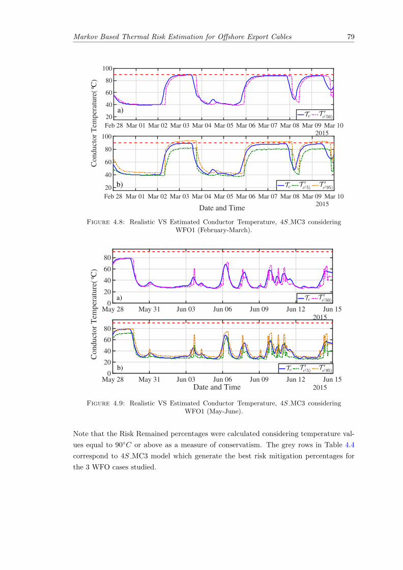
Markov Based Thermal Risk Estimation for Offshore Export Cables 79
Feb 28 Mar 01 Mar 02 Mar 03 Mar 04 Mar 05 Mar 06 Mar 07 Mar 08 Mar 09 Mar 10
2015
20
40
60
80
100
Feb 28 Mar 01 Mar 02 Mar 03 Mar 04 Mar 05 Mar 06 Mar 07 Mar 08 Mar 09 Mar 10
2015
20
40
60
80
100
Date and Time
Condu
cto
r T
emper
ature
(°C
)
b)
a)
Figure 4.8: Realistic VS Estimated Conductor Temperature, 4S MC3 consideringWFO1 (February-March).
May 28 May 31 Jun 03 Jun 06 Jun 09 Jun 12 Jun 15
2015
0
20
40
60
80
May 28 May 31 Jun 03 Jun 06 Jun 09 Jun 12 Jun 15
2015
0
20
40
60
80
Date and Time
Co
nd
uct
or
Tem
per
atu
re(°
C)
b)
a)
Figure 4.9: Realistic VS Estimated Conductor Temperature, 4S MC3 consideringWFO1 (May-June).
Note that the Risk Remained percentages were calculated considering temperature val-
ues equal to 90C or above as a measure of conservatism. The grey rows in Table 4.4
correspond to 4S MC3 model which generate the best risk mitigation percentages for
the 3 WFO cases studied.
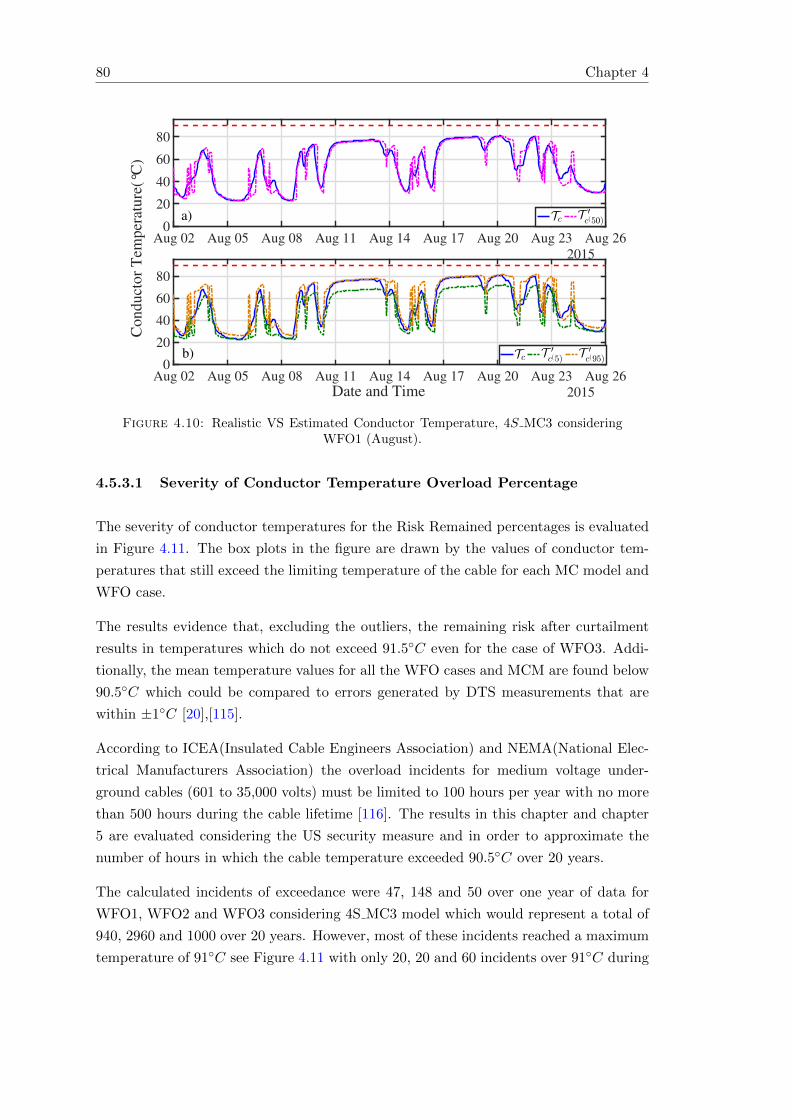
80 Chapter 4
Aug 02 Aug 05 Aug 08 Aug 11 Aug 14 Aug 17 Aug 20 Aug 23 Aug 26
2015
0
20
40
60
80
Aug 02 Aug 05 Aug 08 Aug 11 Aug 14 Aug 17 Aug 20 Aug 23 Aug 26
2015
0
20
40
60
80
Date and Time
Co
nd
uct
or
Tem
per
atu
re(°
C)
b)
a)
Figure 4.10: Realistic VS Estimated Conductor Temperature, 4S MC3 consideringWFO1 (August).
4.5.3.1 Severity of Conductor Temperature Overload Percentage
The severity of conductor temperatures for the Risk Remained percentages is evaluated
in Figure 4.11. The box plots in the figure are drawn by the values of conductor tem-
peratures that still exceed the limiting temperature of the cable for each MC model and
WFO case.
The results evidence that, excluding the outliers, the remaining risk after curtailment
results in temperatures which do not exceed 91.5C even for the case of WFO3. Addi-
tionally, the mean temperature values for all the WFO cases and MCM are found below
90.5C which could be compared to errors generated by DTS measurements that are
within ±1C [20],[115].
According to ICEA(Insulated Cable Engineers Association) and NEMA(National Elec-
trical Manufacturers Association) the overload incidents for medium voltage under-
ground cables (601 to 35,000 volts) must be limited to 100 hours per year with no more
than 500 hours during the cable lifetime [116]. The results in this chapter and chapter
5 are evaluated considering the US security measure and in order to approximate the
number of hours in which the cable temperature exceeded 90.5C over 20 years.
The calculated incidents of exceedance were 47, 148 and 50 over one year of data for
WFO1, WFO2 and WFO3 considering 4S MC3 model which would represent a total of
940, 2960 and 1000 over 20 years. However, most of these incidents reached a maximum
temperature of 91C see Figure 4.11 with only 20, 20 and 60 incidents over 91C during

Markov Based Thermal Risk Estimation for Offshore Export Cables 81
WFO Case MCM Risk Mitigated Risk Remained
WFO1
4S MC1 98.37% 1.62%
4S MC3 98.42% 1.55%
8S MC1 94.49% 5.50%
8S MC3 94.45% 5.51%
17S MC1 95.13% 4.86%
17S MC3 94.87% 5.10%
WFO2
4S MC1 95.89% 4.10%
4S MC3 96.04% 3.92%
8S MC1 92.51% 7.48%
8S MC3 92.52% 7.44%
17S MC1 93.43% 6.56%
17S MC3 93.46% 6.51%
WFO3
4S MC1 97.96% 2.03%
4S MC3 98.24% 1.73%
8S MC1 92.33% 7.66%
8S MC3 92.03% 7.93%
17S MC1 94.75% 5.24%
17S MC3 94.29% 5.67%
Table 4.4: After Online Curtailment Evaluation
4S_M
C1
4S_M
C3
8S_M
C1
8S_M
C3
17S_M
C1
17S_M
C3
4S_M
C1
4S_M
C3
8S_M
C1
8S_M
C3
17S_M
C1
17S_M
C3
4S_M
C1
4S_M
C3
8S_M
C1
8S_M
C3
17S_M
C1
17S_M
C3
MC-Model
90
90.5
91
91.5
92
92.5
93
Conduct
or
Tem
per
ature
(°C
)
WFO1
WFO2
WFO3
Figure 4.11: Analysis of conductor temperature for the Risk Remained in Table 4.4.
the cable lifetime. Additional conservatism can be induced by reducing the cable max-
imum temperature in the algorithm to a value less than 90C i.e. 88 C which would
reduce/eliminate the number of cable thermal exceedances.

82 Chapter 4
4.5.3.2 Estimated Vs Realistic Conductor Temperature Profiles
Figures 4.12, 4.13 and 4.14 part a) present the conductor temperature profile Tc for
the case of WFO3 (4S MC3) along the incidents (represented by * in black) where the
offline methodology estimates a forward temperature exceedance (R′) while Figures 4.12,
4.13 and 4.14 part b)show the temperature profile Tcnew obtained considering the online
estimation and curtailment.
Figure 4.14-b shows that if action is performed when the offline methodology estimates
a forward risk R′ the risk of exceeding the Tlimit is mitigated in 98.24% of cases while
the remaining risk does not exceed 91C as shown in Figure 4.11.
Jan Feb Mar Apr May Jun Jul Aug Sep Oct Nov Dec Jan
2015
20
40
60
80
100
Jan Feb Mar Apr May Jun Jul Aug Sep Oct Nov Dec Jan
2015
20
40
60
80
100
Date and Time
Co
nd
uct
or
Tem
per
atu
re(°
C)
b)
a)
Figure 4.12: Offline VS Online Conductor Temperatures for WFO1, 4S MC3.
The approximate amount of additional power that could be transferred by the cables
was derived from the online simulation as the difference between the base case power
PB and the new profile of power Pnew calculated considering online curtailment during
the year of testing.
4.5.4 Offline and Online Simulation Results: DS2
The results in this section were obtain considering DS2 and the 4S MC3 model for
the 3 WFO cases. The results of the MAE and RMSE for thermal risk and conductor
temperature are both shown in Figure 4.15 distinguished by the subindex R and T .
The calculated MAE R lie between 0.0061 and 0.0277 while RMSE R lie between 0.068
and 0.1367 for the corresponding cases of WFO1 and WFO3. For the case of MAE T the

Markov Based Thermal Risk Estimation for Offshore Export Cables 83
Jan Feb Mar Apr May Jun Jul Aug Sep Oct Nov Dec Jan
2015
20
40
60
80
100
Jan Feb Mar Apr May Jun Jul Aug Sep Oct Nov Dec Jan
2015
20
40
60
80
100
Date and Time
Conduct
or
Tem
per
ature
(°C
)
a)
b)
Figure 4.13: Offline VS Online Conductor Temperatures for WFO2, 4S MC3.
Jan Feb Mar Apr May Jun Jul Aug Sep Oct Nov Dec Jan
2015
20
40
60
80
100
120
Jan Feb Mar Apr May Jun Jul Aug Sep Oct Nov Dec Jan
2015
20
40
60
80
100
Date and Time
Conduct
or
Tem
per
ature
(°C
)
a)
b)
Figure 4.14: Offline VS Online Conductor Temperatures for WFO3, 4S MC3.
maximum and minimum error values were between 4.793C and 5.547C while RMSE T
values were between 7.795C and 8.891C for WFO1 and WFO3 respectively.
These results compared to results obtained using DS1 generate lower values of error
related only to the historical data set from the studied offshore location. For instance, it
was noticed that the profile of wind speed during the winter months at the beginning and
end of the testing year in DS2 was not as strong as in DS1 which in this case generate
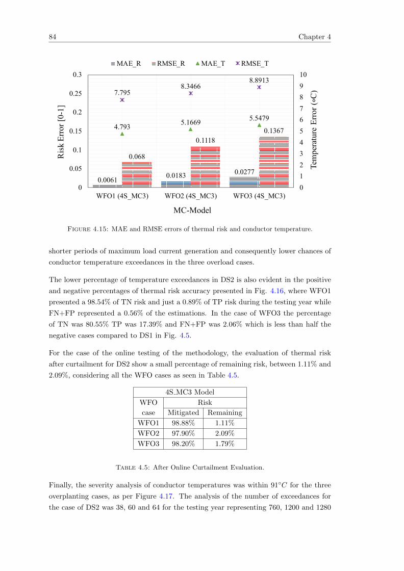
84 Chapter 4
0.00610.0183
0.0277
0.068
0.1118
0.13674.793
5.16695.5479
7.7958.3466
8.8913
0
1
2
3
4
5
6
7
8
9
10
0
0.05
0.1
0.15
0.2
0.25
0.3
WFO1 (4S_MC3) WFO2 (4S_MC3) WFO3 (4S_MC3)
Tem
per
ature
Err
or
(!C
)
Ris
k E
rror
[0-1
]
MC-Model
MAE_R RMSE_R MAE_T RMSE_T
Figure 4.15: MAE and RMSE errors of thermal risk and conductor temperature.
shorter periods of maximum load current generation and consequently lower chances of
conductor temperature exceedances in the three overload cases.
The lower percentage of temperature exceedances in DS2 is also evident in the positive
and negative percentages of thermal risk accuracy presented in Fig. 4.16, where WFO1
presented a 98.54% of TN risk and just a 0.89% of TP risk during the testing year while
FN+FP represented a 0.56% of the estimations. In the case of WFO3 the percentage
of TN was 80.55% TP was 17.39% and FN+FP was 2.06% which is less than half the
negative cases compared to DS1 in Fig. 4.5.
For the case of the online testing of the methodology, the evaluation of thermal risk
after curtailment for DS2 show a small percentage of remaining risk, between 1.11% and
2.09%, considering all the WFO cases as seen in Table 4.5.
4S MC3 Model
WFO Risk
case Mitigated Remaining
WFO1 98.88% 1.11%
WFO2 97.90% 2.09%
WFO3 98.20% 1.79%
Table 4.5: After Online Curtailment Evaluation.
Finally, the severity analysis of conductor temperatures was within 91C for the three
overplanting cases, as per Figure 4.17. The analysis of the number of exceedances for
the case of DS2 was 38, 60 and 64 for the testing year representing 760, 1200 and 1280

Markov Based Thermal Risk Estimation for Offshore Export Cables 85
98.54
89.75
80.55
0.8
9 9.2
5 17.3
9
0.5
2
0.7
8
1.2
3
0.0
3
0.2 0.8
22
0
20
40
60
80
100
120
WFO1 (4S_MC3) WFO2 (4S_MC3) WFO3 (4S_MC3)
% E
stim
ated
Ris
k
MC-Model
True Negative True Positive False Negative False Positive
Figure 4.16: Percentage of positive and negative thermal risk estimations.
over the cable lifetime for WFO1, WFO2 and WFO3 respectively. The severity of these
incidents was mostly below 91C as seen in Figure 4.17 with only 20 incidents above
91C over 20 years for the case of WFO3.
4S_MC3 4S_MC3 4S_MC3
MC-Model
90
90.5
91
91.5
Co
nd
uct
or
Tem
per
atu
re (°C
) WFO1
WFO2
WFO3
Figure 4.17: Analysis of conductor temperature exceedances for remaining thermalrisk in Table 4.5.

86 Chapter 4
4.6 Results comparison MCS based vs MC based TRE
Table 4.6 presents a comparison of the percentage of positive and negative thermal risk
identification obtained from the application of the Methodology in Chapter 4 and this
Chapter, categorised as per Table 3.7.
The best results from the application of the methodologies are compared which for the
case of Chapter 4 correspond to the 5 years training set and the 6 hours ahead estimation
window for DS1 while for the case of this Chapter correspond to the 4S MC3Markov
Chain model considering 5 years of training data and 6 hours ahead estimation for DS1
both methodologies using year 2015 as testing year. The results considering DS2 are
also compared as they follow the selection of 4S MC3 as the most accurate model.
The main objective was the reduction of the False Positive (FP) misclassification cases
which were achieved considering the three overprinting cases.
The additional benefits achieved from the use of the Markov Chain study was the ability
to generate a conductor temperature estimation as seen in figures 4.8, 4.9 and 4.10. The
ability of the non-parametric approach to adapt the estimated TPM to a new set of
data and finally, the online application of the methodology developed for the MC based
methodology was able to mitigate and minimise the existent thermal risk in the cable
system as presented in Tabel 4.4 and 4.5.
4.7 Effect of Charging Current in the Cable
The submarine section of the cable used represents the middle section of the export
system studied (25km offshore), which would reflect almost no charging current impact
considering reactive compensation at both ends of the cable route. The maximum reac-
tive current at one end of the cable would be 5 A/km×50 km = 250 A in the worst-case
scenario thus, considering a full-load continuous rating Is = 923 A the reactive current
would lead to an increased current Ic1 = 931 A (≤ 1%) without compensation.
Charging current effects would vary according to the case studied depending on; the
type of cable, operating voltage, cable length, location of the reactive compensation,
and point of estimation in the transmission line (landfall, submarine sections, offshore
end). Thus, depending on the particular case, charging current effects must be calculated
and added to the load current profile data.
The addition of the charging current into the load current profile would limit the min-
imum value of load current that is possible to reach, thus, the calculated probabilities
in the TPM’s would change if the lower state(s) of the system become(s) less probable
or physically impossible to attain. However, the thermal risk estimation methodology

Markov Based Thermal Risk Estimation for Offshore Export Cables 87
WFO case Category
MCS based TRE MC based TRE MC based TRE
DS1 DS1 DS2
% % %
WFO1
TN 87.28 90.54 98.55
TP 11.65 8.38 0.89
FN 0.36 0.69 0.52
FP 0.69 0.39 0.03
(TN+TP) 98.93 98.92 99.44
(FP+FN) 1.06 1.08 0.56
WFO2
TN 74.76 76.48 89.75
TP 21.87 20.24 9.25
FN 0.62 2.23 0.79
FP 2.72 1.05 0.21
(TN+TP) 96.64 96.72 99.00
(FP+FN) 3.35 3.28 1.00
WFO3
TN 62.14 64.74 80.55
TP 31.29 30.96 17.39
FN 0.799 1.11 1.23
FP 5.756 3.19 0.83
(TN+TP) 93.44 95.7 97.94
(FP+FN) 6.55 4.3 2.06
Table 4.6: Chapter 4 vs chapter 5 results comparison.
would not be affected given that the statistical analysis of the data performed by the
MCM would automatically reflect the changes performed to the given set of data. Fi-
nally, the number of additional wind turbines that could be connected to the cable will
be affected, thus, WFO cases (also induced in the data) must be adjusted according to
the studied cable system.
4.8 Summary
The methodology presented for the forward thermal risk estimation applied to wind
farm export cables considered uncertainty in power generation. Future likely conductor
temperatures in the system were estimated through the use of monthly TPM derived
from 5 years of data MCS and the finite-difference model of the cable. Six Markov models
with a different number of system states and higher-order TPM’s were developed, tested
and evaluated.
Overplanting cases induced the risk of the cable exceeding 90C and the methodology
proved to generate a high percentage of successful identifications of risk 6h ahead from
95.68% in WFO3 to 98.09% in WFO1 during one year of offline testing with MAE of
0.0158 and 0.0419 respectively. An online application of the methodology including

88 Chapter 4
a simulated curtailment strategy generated a high percentage of thermal risk mitiga-
tion while analysis the remaining percentage of thermal exceedances did not exceed a
temperature higher than 91.5C for DS1 and 91C for DS2.
The additional power delivery obtained was 7.26%, 9.16% and 9.67% per year compared
to the traditional limiting rating based on IEC60287 (1149.58 GWh/year). The calcu-
lated approximate revenue that the additional power could represent for the wind farm
project is 6.05, 7.63 and 8.06 million £/year for DS1. Tests performed in two datasets
from different offshore locations proved that the statistically based method is easy to
use, non-restrictive or parametric to a specific set of data.
The results obtained from the temperature error analysis in Figure 4.7 showed medium
to high overestimations or underestimations of conductor temperatures during periods of
high↔low load current transition. The evidence opened the research question regarding
the use of a ramp rate study to anticipate the load current transitions and the effects
that they produce in the cable system. The topic is addressed in Chapter 5.
The journal paper entitled “Cable Thermal Risk Estimation for Overplanted Wind
Farms” containing the methodology and results presented in this Chapter was writ-
ten and accepted for publication in the IEEE Transactions on Power Delivery on 20th
of May 2019 [117].

Chapter 5
Export Cable Thermal Risk
Management via Ramp
Identification
The overestimations and underestimations found in the results in chapter 4 were lo-
cated at times of fast power variations, thus, following an evaluation of the literature, a
ramp event identification approach was developed to target this issue, and the obtained
results are presented in this chapter.
An introduction to the topic of wind power ramp forecasting is first presented, followed
by the explanation of the proposed algorithm, cable system (example 2) and overplanting
scenarios used to evaluate the method. The submarine cable system presented here was
extended to include the limiting section of the cable, thus, the submarine and landfall
sections are both monitored.
Contrarily to the algorithm in chapter 4 the present investigation focused solely on
the study of fast power variations (ramp events) in the historical load current data to
investigate if the novel approach can improve the results obtained by MC based TRE
methodology.
A classification method was used to study, characterise and identify load current ramps
separately, rather than focusing on estimating the whole future load current profile [17].
The identification of power ramps duration and magnitude is used to estimate their
thermal consequences in the export cable and plan if a likely risk of cable overheating is
foreseen. Finally, the TRE results obtained are compared to the results obtained from
the MC based methodology in chapter 4.
89

90 Chapter 5
5.1 Introduction to Wind Power Ramp Forecasting
Ramp events can be generally described as large increments/decrements in power gen-
eration which can cause power system imbalance, loss of power and increments in cable
temperatures in transmission systems with integrated variable energy sources. Due to
the increasing interconnection of renewable energy sources into the electric grids, wind
power identification, estimation and forecasting have become a new area of research.
Wind Power Ramp Forecasting has been especially focused to deal with the management
of wind power variation in systems with high penetration [99, 118]. The investigation
presented by Gallego-Castillo et al. in [17] summarises recent works related to wind
power ramp event forecasting. The review evidences how the interest in the investigation
of large and fast variations of wind power has boomed since 2007 into a noticeable number
of JCR articles.
The definition of a ramp event has not been clearly defined or standardised in the
literature, however, the general ramp characteristics found are; magnitude, duration,
ramp rate, direction and the selection of a certain threshold value th. In this thesis,
a ramp event is identified defined as more than consecutive increments (±) below a
selected load current threshold th defined as seen later in section 5.2.1.
Additionally, the available literature shows a wide variety of approaches to target the
issue such as ramp alarms, statistical characterisation of ramp events and, forecasting
of ramp features such as ramp rates. Finally, the explanatory variables and parameters
involved in the methodologies have been described as complex and not easy to generalise
given to their underlying meteorological and geographical nature [17].
A representative example of ramp events is presented in Figure 5.1 where up (red) and
down (green) ramps are highlighted for the load current data in DS1 during January
1996. In this Chapter, the proposed approach makes use of clustered analysis of load
current ramp rates derived from the analysis of historical ramp events in the data to
identify future ramps and perform an hour ahead estimation of thermal risk in the cable
given the ramp direction and intensity.
5.2 Ramp Identification Based TRE Methodology
The overview of the novel thermal risk estimation algorithm is summarised in Figure
5.2. The methodology starts with the historical data analysis and classification of load
current ramp rates (Steps A and B) which are performed only once given the case study:
cable size, WFO case, and historical dataset.
The subsequent steps C, D and E are performed at every time step considering updates
in cable load current I(t). The methodology can be used as an online/offline tool as seen

Export Cable Thermal Risk Management via Ramp Identification 91
Jan 03 Jan 04 Jan 05 Jan 06 Jan 07
Date and time 1996
0
100
200
300
400
500
600
700
800
Load
Curr
ent
(A)
Ramp event 3
Ramp event 4
Ramp event 1
Ramp event 6
Ramp event 7
Figure 5.1: Load current profile and selected threshold value th1, red dotted line.
in Figure 5.2 where the black blocks represent the offline application and the addition
of the blue steps represent the online application tool. The methodology steps are
individually explained below.
5.2.1 Analysis of historical load current ramp events
Let the load current generation at time t and t+ ∆t be I(t) and I(t+ ∆t) respectively.
The time interval ∆t here is one hour given by the sampling step in the wind speed
dataset. The analysis of the historical data starts by computing the difference between
the consecutive values of load current data given by
∆L = I(t+ ∆t)− I(t) (5.1)
where the sign of ∆L indicates the direction of the increment (positive/negative).
A ramp event is identified by the algorithm as the consecutive increments (±∆L) below
a load current threshold th. The load current value th draws the boundary between a
high to full load current (over th) and the ramp event zone (below th) thus its selection
is case dependent and must be defined after the analysis of the studied data.
The magnitude of a ramp event (∆k) is given by I(t) which represents the load current
at the identified beginning of the ramp and I(t+∆k) which is the load current at the end
of the ramp. Thus the values of ramp duration (∆k) and magnitude (I(t+∆k)−I(t)) are
obtained for each identified ramp in the historical data and stored for further analysis.
According to the durations of ramps found during the ramp event analysis, an inter-
val [α, β] (hours) is chosen to define the relevant ramp events for the studied dataset.

92 Chapter 5
FDMmain
D. Calculate T (t)I(t)
C. Ramp Iden-tification and
expected Ie(t+u)
A. Load cur-rent data analysis
B. Classification of Rrate
Historicalload currentdataset I(t)
Start
C. MCS generatesIsample(i×u)(t)
FDMsub
D. CalculateT ′(i×u)(t) and pdfT ′(t)
t = t+ u
E. Calculateerisk / erisk2
Thermal riskCurtailment
I(t) = IB(t+ 1)
yes
I(t) = I(t + 1)
no
E. Calculaterrisk / rrisk2
yes
no
Figure 5.2: Ramp based TRE methodology, flowchart.
The historical ramp events with duration in the interval [α, β] are studied monthly to
calculate the ramp rate Rrate of the individual ramps as
Rrate =I(t+ ∆k)− I(t)
∆k(A/h) (5.2)
where the resulting Rrate is given in Amperes per hour and represents the average hourly
rate of change (±) of load current.
The selected values for parameters th, α and β are presented in Section 5.7 as well as
the procedure for its selection regarding the case study and general guidelines for its
selection for a different set of data.
Finally, Section 5.3 presents a data analysis example which would clarify how to select
some parameters used in this section i.e. α and β, however, the rest of the algorithm
steps must first be explained to understand the extraction of the ramp rate features.
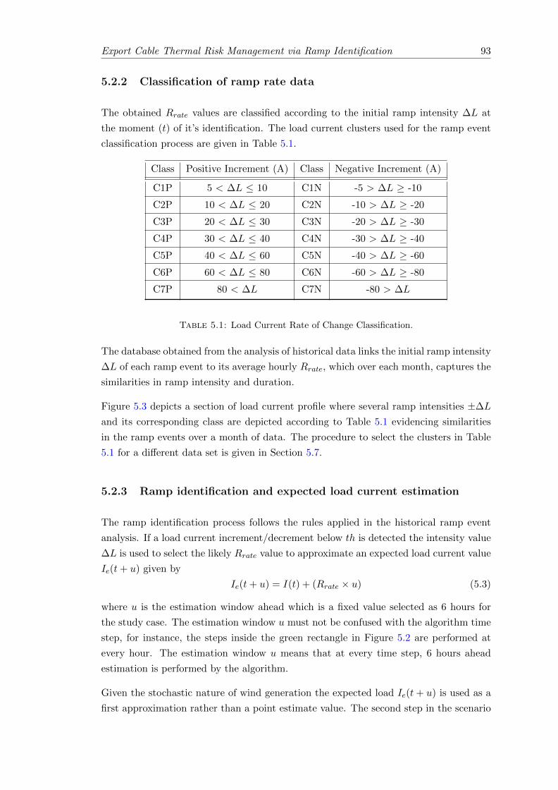
Export Cable Thermal Risk Management via Ramp Identification 93
5.2.2 Classification of ramp rate data
The obtained Rrate values are classified according to the initial ramp intensity ∆L at
the moment (t) of it’s identification. The load current clusters used for the ramp event
classification process are given in Table 5.1.
Class Positive Increment (A) Class Negative Increment (A)
C1P 5 < ∆L ≤ 10 C1N -5 > ∆L ≥ -10
C2P 10 < ∆L ≤ 20 C2N -10 > ∆L ≥ -20
C3P 20 < ∆L ≤ 30 C3N -20 > ∆L ≥ -30
C4P 30 < ∆L ≤ 40 C4N -30 > ∆L ≥ -40
C5P 40 < ∆L ≤ 60 C5N -40 > ∆L ≥ -60
C6P 60 < ∆L ≤ 80 C6N -60 > ∆L ≥ -80
C7P 80 < ∆L C7N -80 > ∆L
Table 5.1: Load Current Rate of Change Classification.
The database obtained from the analysis of historical data links the initial ramp intensity
∆L of each ramp event to its average hourly Rrate, which over each month, captures the
similarities in ramp intensity and duration.
Figure 5.3 depicts a section of load current profile where several ramp intensities ±∆L
and its corresponding class are depicted according to Table 5.1 evidencing similarities
in the ramp events over a month of data. The procedure to select the clusters in Table
5.1 for a different data set is given in Section 5.7.
5.2.3 Ramp identification and expected load current estimation
The ramp identification process follows the rules applied in the historical ramp event
analysis. If a load current increment/decrement below th is detected the intensity value
∆L is used to select the likely Rrate value to approximate an expected load current value
Ie(t+ u) given by
Ie(t+ u) = I(t) + (Rrate × u) (5.3)
where u is the estimation window ahead which is a fixed value selected as 6 hours for
the study case. The estimation window u must not be confused with the algorithm time
step, for instance, the steps inside the green rectangle in Figure 5.2 are performed at
every hour. The estimation window u means that at every time step, 6 hours ahead
estimation is performed by the algorithm.
Given the stochastic nature of wind generation the expected load Ie(t+ u) is used as a
first approximation rather than a point estimate value. The second step in the scenario

94 Chapter 5
Mar 21 Mar 23 Mar 25 Mar 27 Mar 29 Mar 31
Date and Time 1996
0
100
200
300
400
500
600
700
800
900L
oad C
urr
ent
(A)
I(t)
th
C7N
C3P
C7NC7N
C3P
C2P
C2P
C7P
C7N
C7N
C7N
C1P
Figure 5.3: Load current profile and selected threshold value th.
sampling makes use of MCS to generate likely series of load current scenarios in the
vicinity of the expected load Ie(t + u). The scenario sampling algorithm is formulated
as
evalue = icdf(pdf, Ie(t+ u));
rmax = evalue + γ;
rmin = evalue − γ;
rnum(i× u) = (rmax − rmin)× rand(i, u) + rmin;
Isample(i× u) = icdf(pdf, rnum).
where evalue is the probability value of the expected load Ie(t+u) in the data probability
distribution (pdf) calculated by the inverse cumulative distribution method (icdf); γ is
the uncertainty value selected as the probability range in which the MCS would be
allowed above and below evalue; rnum is the matrix of random numbers used to obtain
the load current matrix Isample from the icdf ; i represents the number of series of samples
desired for the sampling process and; u is the hours ahead estimation window.
The selected values for parameters γ and i are presented in Section 5.7 along with general
guidelines for its selection considering a different dataset.
5.2.4 Dynamic conductor temperature calculation
The submarine cable thermo-electric equivalent model was taken from [34] (see section
3.4) and is solved via FDM to obtain the conductor temperature. Nevertheless, the

Export Cable Thermal Risk Management via Ramp Identification 95
proposed algorithm is independent of the cable model thus choosing a different cable
model would not affect the steps in the TRE framework.
The calculation of realistic conductor temperatures at every time step (t) is given by
the main routine (FDMmain) while the subroutine (FDMsub) calculates the conductor
temperature considering the sampled future load current series Isample.
Both calculations run in parallel as shown in Figure 5.2. For instance, the conductor
temperature T (t) given by FDMmain is used as initial condition for the conductor tem-
perature calculations T ′(i×u)(t) in FDMsub. Thus, the estimated conductor temperatures
T ′(i×u)(t) represent the likely temperatures of the conductor if load current similar to the
sampled are present in the cable in the following hours.
The estimated temperatures are used to create a probability distribution function of
likely conductor temperatures (pdfT ′(t)) at every time step which is used by the subse-
quent estimation of likely thermal risk in the cable system.
5.2.5 Offline thermal risk estimation
The hours ahead likely temperatures distribution is used to calculate the likely thermal
risk (erisk) that the cable could face in the following hours as
erisk =T ′(t+ 1, t+ 2....t+ u) ≥ Tlimit
u(5.4)
where T ′(t+ 1, t+ 2....t+ u) ∈ pdfT ′(t) represent the most likely series of load current
values in the sampled distribution considering the median of the sampled pdfT ′(t).
The realistic risk rrisk is calculated in order to evaluate the estimated risk in a similar
way as erisk, for instance
rrisk =T (t+ 1, t+ 2....t+ u) ≥ Tlimit
u(5.5)
where T (t+ 1, t+ 2....t+ u) are the conductor temperatures obtained by the FDMmain.
The calculation of rrisk is obtained 6 hours after, when the relevant data is available for
comparison.
5.2.6 Online thermal risk estimation and curtailment
The difference between the online and offline simulation is the application of a preventive
curtailment if the online simulation estimates a thermal risk 6h ahead in Figure 5.2 black
plus blue steps.

96 Chapter 5
For instance, if a thermal risk is estimated the next load current value data in the
FDMmain is reduced according to the base case wind farm for the next hour thus I(t) =
IB(t+ 1). This power reduction simulates the decision of the TSO to apply a constraint
in power to avoid thermal damage to the cable.
The simulated curtailment modifies the load current data set as necessary to avoid
exceeding the cable temperature limit. Considering the updated load current a new
estimated thermal risk erisk2 and new the realistic risk rrisk2, are calculated similarly as
in equations (5.4) and (5.5).
The non-curtailed risks erisk and rrisk are also calculated for comparison. The calculation
of both online and offline estimated/realistic risks are used for the evaluation of the
methodology which is explained in the following section.
5.2.7 Methodology evaluation process
Offline and online simulations were carried out following the testing procedure described
in Section 5.2. The methodology evaluation steps described below follows a similar
process compared to Chapter 4 for results comparison.
The hourly estimated thermal risk erisk and realistic risk rrisk calculated over one year
of testing are stored and compared considering the classification cases in Table 3.7 where
the realistic thermal risk r is given by rrisk and the estimated risk r is represented by
erisk.
The binary evaluation accounts for the accuracy of the methodology to estimate likely
thermal risk 6h ahead while MAE and RMSE calculate the average error between the
estimated thermal risk (erisk) and the realistic thermal risk (rrisk). MAE is proportion-
ally affected by the absolute error between the variables while in RMSE the square root
of errors gives more weight to large errors.
The preventive curtailment carried out during the online simulation is given by the
reduction of the load current profile Imax (for the given WFO case) to the BWF rating
for the following hour. The applied curtailment is a conservative example that can be
extended over longer periods as required by the user/study case.
The online methodology evaluation involves the comparison of the actual risk rrisk (un-
curtailed case) and the online estimated risk erisk2 calculated after the preventive cur-
tailment action. The classes and sub-classes used for the evaluation of the online TRE
and curtailment results are given in detail in Table 4.3 where R(t) is now given by rrisk
and Rnew(t) is substituted by erisk2.

Export Cable Thermal Risk Management via Ramp Identification 97
5.3 Ramp Event Data Analysis
An example of the ramp analysis study described in steps A and B of Figure 5.2 are
applied in this section considering a 9.9% wind farm overplanting and the results are
presented to demonstrate how the data analysis is performed. The algorithm in this
Chapter is trained using the first 5 years of load current data from DS1 (1996-2000)
while the testing is done using the year 2015 from the same dataset.
The analysis of positive and negative ramp duration extracted from the training set
is presented for each month in Fig. 5.4. The box edges indicate the 25th and 75th
percentiles, the central red line indicates the median ramp duration for the month, the
bottom and top whiskers extend to the most extreme duration times not considering
outliers, which, are represented by the (*) symbol. The outliers are defined as done for
the case of Figure 3.1.
Jan Feb Mar Apr May Jun Jul Aug Sep Oct Nov Dec
Month
4
6
8
10
12
14
+ R
amp D
ura
tion (
h)
Jan Feb Mar Apr May Jun Jul Aug Sep Oct Nov Dec
Month
5
10
15
20
- R
amp D
ura
tion (
h)
Figure 5.4: Ramp events duration in hours for each month.
Figure 5.4 shows that the mean average values of positive ramps are within 5.5 and 7
hours, while the duration of negative ramps is between 6 and 7 hours. Thus, the selected
u=6h represents the ideal estimation window for the data set studied.
Considering the 75th percentiles values and the most extreme incidences, it is found that
positive ramp dynamics are faster than negative ramps. Therefore, fast identification of
positive ramps and the estimation of its thermal consequences in the cable is important
to manage thermal risk.

98 Chapter 5
The number of ramp events identified by the ramp analysis process for the studied 5
years of historical data is presented in Figure 5.5.
0 1 2 3 4 5 6 7 8 9 10 11 120
50
100
150
Po
siti
ve
Ram
p
1 2 3 4 5 6 7 8 9 10 11 12Month
0
50
100
150
Neg
ativ
e R
amp
104
118 121129
154149
109
7183 83
77
58
6556
79
113119
113 134
151
99
64
81 78
Figure 5.5: Total number of identified ramp events during the data analysis, by monthfor a 5 year period.
During October to March, the frequency of ramp events is much lower than for the rest
of the year due to more stable high to full load generation levels. On the other hand,
the higher number of ramp variations during warmer months of the year reflects more
load current variations in a medium to low load current generation level.
Figure 5.6 presents the results of the positive and negative Rrate classification process
for March (red boxes) and July (blue boxes) considering the categories as per Table 5.1.
The box plot edges in Figure 5.6 indicate the 25th and 75th percentiles and the median
ramp Rrate for each class is the central red line whose values are plotted in both figures
for reference. Finally, the black whiskers are the most extreme values found for the case
and the outliers are represented by the (*) symbol and calculated as explained for Figure
3.1.
The obtained Rrate values show the ability of the method to extract and classify historical
ramp events information which is subsequently used to perform estimations regarding
the future thermal state of the cable system.
5.4 Cable System Design Example 2
The studied cable system consists of a 132 kV 3-core XLPE insulated cable, 800mm2
copper conductor for the submarine section and 132 kV 3-core XLPE insulated cable,

Export Cable Thermal Risk Management via Ramp Identification 99
C1P C1P C2P C2P C3P C3P C4P C4P C5P C5P C6P C6P C7P C7P
Positive Class
0
50
100
150
200March
July
C1N C1N C2N C2N C3N C3N C4N C4N C5N C5N C6N C6N C7N C7N
Negative Class
-150
-100
-50
0
March
July
22.08
16.95
37.73
29.5645.85
45.02
76.0449.53
94.6048.91
106.31
-56.18-57.63
-24.60
103.58
58.97
-35.79
-35.75
-19.42 -21.73
-23.35
-9.23 -32.37
-35.25 -29.38
-86.72
112.66
-80.54
Figure 5.6: Calculated ramp rate values for the month of March (red) and July (blue).
1400mm2 copper conductor for the landfall section, see Figure 5.7, both with a maximum
temperature limit of Tlimit =90C.
The submarine section (TS1), has a 1000 mm burial depth and 0.7 KmW−1 soil thermal
resistivity while the landfall section (TS2), has a 4000 mm burial depth and 1.0 KmW−1
soil thermal resistivity. The water temperature is set as 15C in both cases, representing
the maximum value of ambient temperature for the studied offshore location in the North
Sea.
The TRE algorithm was tested by estimating the conductor temperature of the two
thermal sections knowing beforehand that the landfall is the thermally limiting section
of the cable system.
132:33kV400:132kV
Submarine
Section
Land
CableLandfall
Section
Wind Turbines Array
Figure 5.7: Cable system one-line diagram.
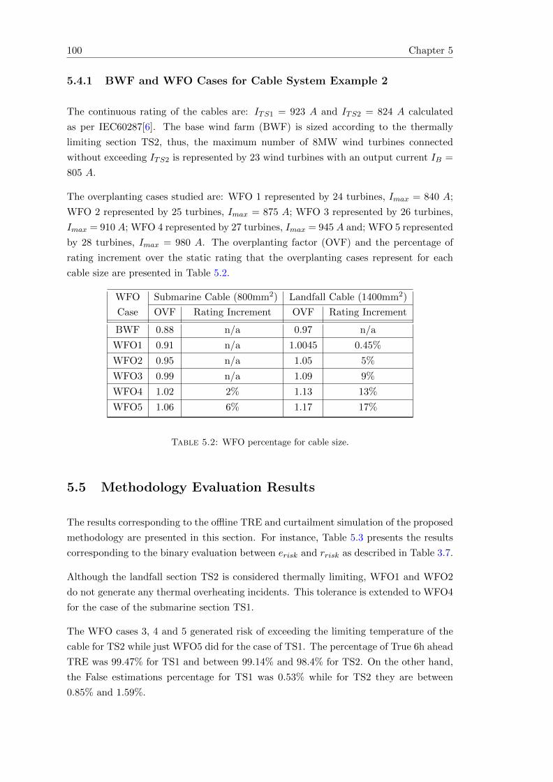
100 Chapter 5
5.4.1 BWF and WFO Cases for Cable System Example 2
The continuous rating of the cables are: ITS1 = 923 A and ITS2 = 824 A calculated
as per IEC60287[6]. The base wind farm (BWF) is sized according to the thermally
limiting section TS2, thus, the maximum number of 8MW wind turbines connected
without exceeding ITS2 is represented by 23 wind turbines with an output current IB =
805 A.
The overplanting cases studied are: WFO 1 represented by 24 turbines, Imax = 840 A;
WFO 2 represented by 25 turbines, Imax = 875 A; WFO 3 represented by 26 turbines,
Imax = 910 A; WFO 4 represented by 27 turbines, Imax = 945 A and; WFO 5 represented
by 28 turbines, Imax = 980 A. The overplanting factor (OVF) and the percentage of
rating increment over the static rating that the overplanting cases represent for each
cable size are presented in Table 5.2.
WFO Submarine Cable (800mm2) Landfall Cable (1400mm2)
Case OVF Rating Increment OVF Rating Increment
BWF 0.88 n/a 0.97 n/a
WFO1 0.91 n/a 1.0045 0.45%
WFO2 0.95 n/a 1.05 5%
WFO3 0.99 n/a 1.09 9%
WFO4 1.02 2% 1.13 13%
WFO5 1.06 6% 1.17 17%
Table 5.2: WFO percentage for cable size.
5.5 Methodology Evaluation Results
The results corresponding to the offline TRE and curtailment simulation of the proposed
methodology are presented in this section. For instance, Table 5.3 presents the results
corresponding to the binary evaluation between erisk and rrisk as described in Table 3.7.
Although the landfall section TS2 is considered thermally limiting, WFO1 and WFO2
do not generate any thermal overheating incidents. This tolerance is extended to WFO4
for the case of the submarine section TS1.
The WFO cases 3, 4 and 5 generated risk of exceeding the limiting temperature of the
cable for TS2 while just WFO5 did for the case of TS1. The percentage of True 6h ahead
TRE was 99.47% for TS1 and between 99.14% and 98.4% for TS2. On the other hand,
the False estimations percentage for TS1 was 0.53% while for TS2 they are between
0.85% and 1.59%.

Export Cable Thermal Risk Management via Ramp Identification 101
ThermalCase WFO1 WFO2 WFO3 WFO4 WFO5
Section
TS1
TN % 100 100 100 100 85.48
TP% 0 0 0 0 14.0
FN % 0 0 0 0 0.14
FP % 0 0 0 0 0.39
True 100% 100% 100% 100% 99.47%
False 0% 0% 0% 0% 0.53%
TS2
TN% 100 100 83.54 67.25 59.78
TP % 0 0 15.6 31.15 38.62
FN % 0 0 0.23 0.4 0.37
FP % 0 0 0.62 1.19 1.22
True 100% 100% 99.14% 98.4% 98.4%
False 0% 0% 0.85% 1.59% 1.59%
Table 5.3: Offline TRE Results.
The results in Figure 5.8 show the MAE and RMSE between erisk and rrisk. The MAE
and RMSE for TS1 for the case of WFO5 are 0.0089 and 0.0654 while for TS2 the
calculated MAE for WFO3 to 5 were 0.0123, 0.0168 and, 0.0181 while the obtained
RMSE were 0.0738, 0.0857 and, 0.0888 respectively.
WFO 1 WFO 2 WFO 3 WFO 4 WFO 5
WFO case
0
0.01
0.02
0.03
0.04
0.05
0.06
0.07
0.08
0.09
Ris
k e
rror
[0-1
]
MAE TS1
MAE TS2
RMSE TS1
RMSE TS2
Figure 5.8: MAE and RMSE risk error.
Although the purpose of the proposed methodology is not the generation of a point
estimate of conductor temperature, a comparison of the 50th percentile value of the

102 Chapter 5
pdfT ′(t) and the realistic temperature T (t + u) was carried out. The MAE and RMSE
between these values were calculated for the whole year of testing and the results are
shown in Figure 5.9.
WFO 1 WFO 2 WFO 3 WFO 4 WFO 5
WFO case
2
3
4
5
6
7
Tem
per
ature
err
or °C
MAE TS1
MAE TS2
RMSE TS1
RMSE TS2
Figure 5.9: MAE and RMSE temperature error.
The results evidence that even when there is no thermal risk the sampled temperatures
in pdfT ′(t) are close to the realistic 6h ahead cable temperatures. For instance, the MAE
for TS1 was between 3.13C and 4.16C and the RMSE between 5.13C and 6.79C,
considering all WFO. On the other hand, the MAE for TS2 was between 2.48C and
3.32C and RMSE between 3.73C and 4.96C for all WFO.
5.5.1 Online TRE results
Table 5.4 presents the percentages of Mitigated (M) and Remained (R) risk for the case
of an online application of the TRE methodology as per Table 4.3.
Considering TS1 the results show no risk of temperature exceedances for WFO 1 to WFO
4 as previously seen in Table 5.3. On the other hand, WFO 5 presented 85.87% no risk
(NR) and 14.13% of thermal risk mitigated (RM) given the automatic curtailment action
during the year of testing, this is translated as a 100% risk mitigation (NR+RM).
For the landfall section (TS2) the methodology was able to mitigate 99.99%, 99.92% and
82.45% of the thermal risk for the WFO cases 3, 4 and 5 respectively. The high 17.54%
of the remaining risk for case WFO5 in Table 5.4 is a combined result of the overly
aggressive 17% overplanting, the cable thermal dynamics and the curtailment strategy
used in the methodology. The number of incidents over 90C was 20 for WFO3 and 140
for WFO4 over the cable lifetime (20 years).
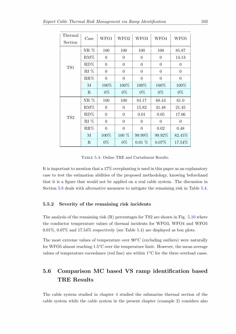
Export Cable Thermal Risk Management via Ramp Identification 103
ThermalCase WFO1 WFO2 WFO3 WFO4 WFO5
Section
TS1
NR % 100 100 100 100 85.87
RM% 0 0 0 0 14.13
RD% 0 0 0 0 0
RI % 0 0 0 0 0
RR% 0 0 0 0 0
M 100% 100% 100% 100% 100%
R 0% 0% 0% 0% 0%
TS2
NR % 100 100 84.17 68.44 61.0
RM% 0 0 15.82 31.48 21.45
RD% 0 0 0.01 0.05 17.06
RI % 0 0 0 0 0
RR% 0 0 0 0.02 0.48
M 100% 100 % 99.99% 99.92% 82.45%
R 0% 0% 0.01 % 0.07% 17.54%
Table 5.4: Online TRE and Curtailment Results.
It is important to mention that a 17% overplanting is used in this paper as an explanatory
case to test the estimation abilities of the proposed methodology, knowing beforehand
that it is a figure that would not be applied on a real cable system. The discussion in
Section 5.8 deals with alternative measures to mitigate the remaining risk in Table 5.4.
5.5.2 Severity of the remaining risk incidents
The analysis of the remaining risk (R) percentages for TS2 are shown in Fig. 5.10 where
the conductor temperature values of thermal incidents for WFO3, WFO4 and WFO5
0.01%, 0.07% and 17.54% respectively (see Table 5.4) are displayed as box plots.
The most extreme values of temperature over 90C (excluding outliers) were naturally
for WFO5 almost reaching 1.5C over the temperature limit. However, the mean average
values of temperature exceedance (red line) are within 1C for the three overload cases.
5.6 Comparison MC based VS ramp identification based
TRE Results
The cable system studied in chapter 4 studied the submarine thermal section of the
cable system while the cable system in the present chapter (example 2) considers also

104 Chapter 5
WFO 3 WFO 4 WFO 5
WFO case
90
90.5
91
91.5
92
92.5
93C
onduct
or
Tem
per
ature
(°C
)
Figure 5.10: Analysis of remaining risk % of conductor temperatures in TS2.
the landfall section of the cable which presents thermally limiting characteristics.
The MC based TRE could correctly identify thermal risk in the cable 6h ahead 95.68%
of the time for a 13% rating increment (WFO3) and 98.09% of the time for a 6% rating
increment (WFO1). In this chapter, the successful percentage of risk identification for
a 6% overplanting (WFO5) in the submarine cable section was 100% considering the
ramp-based method.
Additionally, the percentages of successful thermal risk identifications for WFO3 (9%over-
planting) to WFO5 (17%overplanting) in the thermally limiting landfall section were
between 99.14% and 98.4% which are higher than the above results in chapter 4.
Finally, the percentage of false-positive (FP) identifications of risk in Chapter 4 was
3.19% which considering the ramp-based approach were 1.22% which represent more
than a 50% improvement in a subcategory of false identification that would reduce the
financial benefits for the system.
5.7 Guidelines for parameters selection
Table 5.5 shows the parameters involved in the algorithm. Similarly to most of the works
related to ramp events studies in the literature, these parameters are case dependent and
must be modified according to the studied case [17]. General guidelines for parameter
selection are presented in this section.

Export Cable Thermal Risk Management via Ramp Identification 105
Parameter Definition Value Units
th Load current threshold value 85% Imax Amperes (A)
α and β Studied ramp duration interval 3 and 20 hours (h)
u Estimation window 6 hours (h)
γ Uncertainty value ± 0.1 unit [0-1]
i Sampled series in MCS 500 n/a
Tlimit Maximum cable temperature allowed 90 Celsius (C)
Table 5.5: Selected methodology parameters.
5.7.1 Threshold value th
The load current threshold value th is case-specific and depends on the variability of the
data set studied and the maximum output generation of the wind farm (Imax). In this
study th = Imax× 0.85 defined according to the observation that 87% of the time a 15%
reduction in power generation led to a ramp event in the following hours.
For instance, Figure 5.11 illustrates three ramp event threshold values th1 = 85%Imax,
th2 = 90%Imax and th3 = 95%Imax along the load current profile I(t). The highlighted
areas in green show events that would be confused as ramps if thresholds th2 or th3 were
selected.
Dec 30, 1996 Jan 06, 1997 Jan 13, 1997 Jan 20, 1997 Jan 27, 1997 Feb 03, 1997 Feb 10, 1997
Date and time
0
100
200
300
400
500
600
700
800
Load C
urr
ent
(A)
I(t)
th1=85% I
max
th2=90% I
max
th3=95% I
max
Figure 5.11: Load current profile and selected threshold value th1, red dotted line.
Visual inspection of the datasets studied is an important step in the selection of the
parameters which allows the user to select the desired threshold to reduce false-positive
ramp events such as the ones seen in Figure 5.11.

106 Chapter 5
Finally, selecting a percentage of the installed capacity Imax instead of a fixed output
power value ensures that if the wind farm output is changed the selected th is modified
accordingly [17].
5.7.2 Studied ramp duration interval α and β
The interval values α = 3 and β = 20 were chosen to include events of greater or smaller
time durations in both positive and negative ramp events.
The values α and β can be defined as a close range of ramp durations which would
exclude events of greater or smaller time durations i.e. α = 3 and β = 6. Nevertheless,
in this study, the authors considered the analysis of infrequent but possible long-duration
ramps (25%) while capturing the more frequent short ramps (75%) as seen in Figure
5.4.
5.7.3 Estimation window u and number of MCS iterations i
The selection of u = 6 is selected considering the median value of positive and negative
ramp events in order to choose the ideal estimation window for the data set studied. For
instance, Figure 5.4 shows that the mean average values of positive ramps are within
5.5 and 7 hours, while the duration of negative ramps is between 6 and 7 hours.
The number of samples i for the MCS will influence the accuracy of the estimations thus
it can be increased if desired while accounting for optimisation of the computational time
as the MCS process is carried at every time step.
5.7.4 Uncertainty parameters γ
The uncertainty parameter γ must be approximated given the mean average error be-
tween the estimated load current Ie(t+u) and the realistic load current I(t) considering
one year of estimations, thus γ is given by
γ =
n∑t=1
| I(t)− Ie(t+ u)
Imax| (5.6)
where Imax is the maximum load current output value for the wind farm case studied.
With the uncertainty value defined, the MCS is incorporated in the algorithm considering
a probability range of value γ = ±0.15 around the estimated value Ie(t + u) when
generating the random sampling.

Export Cable Thermal Risk Management via Ramp Identification 107
5.7.5 Load Current Rate of Change Classification
The classification is given by Table 5.1 must be defined according to the corresponding
jumps found in the data analysis. For instance, considering the initial ramp event
intensity ∆L the MATLAB histogram function automatically selects the most appropriate
number of bins and cluster values found in the underlying distribution thus, it is the
selected tool used for the selection of the corresponding classes studied see Figure 5.12.
Figure 5.12: Initial ramp event intensity ∆L found in ramp events DS1.
5.8 Model considerations and charging current effects.
The proposed cable system is a simplified example considering landfall and submarine
cable sections. The cable system, thermal model and ambient parameters can be adapted
to suit specific conditions, for instance, a variable temperature profile could be added to
the framework.
The cable model is not an extension of the proposed methodology thus, the method
can work with any thermal model and a specific cable system that the user may have.
Similarly, the methodology time interval can be changed according to the data time
interval.
Regarding charging current, the model can be deployed at any point along the cable
and thus the charging current must be calculated and added to the load current profile
depending on operating voltage, cable length, location of the reactive compensation.
The addition of a reactive current in the dataset would increase the load current profile
which would not affect the ramp rate study algorithm or the thermal risk estimation

108 Chapter 5
process. Additional conservatism can be induced in the estimations by reducing the
allowed Tlimit in the algorithm which will act as a safety margin to the cable installation
and would help to further reduce the remaining risk for the online application of the
method. Another alternative for the same purpose is the application of an optimised
curtailment strategy i.e. extending the periods of load current reduction in the online
TRE algorithm.
5.9 Summary
A methodology to characterise power generation ramps is proposed for the estimation
of thermal overheating in offshore wind farm cables. A statistical analysis of historical
data is used to extract ramp rate characteristics from the studied dataset to identify
ramps, estimate future load current scenarios and, likely cable temperatures.
The estimated conductor temperatures are used to calculate and prevent the risk of tem-
perature exceedance in the export cable while the application of overplanting scenarios
allows the optimisation of transmission capacity.
The simulated results show a percentage of successful 6h ahead estimations between
99.47% and 98.4% for offline testing. The online application of the methodology was
able to avoid the thermal risk ahead in the range of 99.99% to 82.45% while the remaining
risk percentage generated temperature exceedances with a mean value of 1C over the
allowed 90C.
The additional power delivery of 4.3%, 8.7%, 12.2% and 15.3% per year were achieved
compared to the traditional limiting rating based on IEC60287 (1017 GWh/year). The
results comparison over the methodology presented in Chapter 4 shows an improve-
ment of more than 50% for the false-positive identifications of risk, which represented a
reduction of the financial benefits for the system.
The proposed methodology could be used by the TSO to avoid unnecessary power cur-
tailment in wind farms where overplanting scenarios are applied for economic purposes.
As the algorithm is based on a statistical analysis of historical data collected from initial
site surveys it represents a cost-effective tool that would not induce additional costs as
it does not require the installation of measurement devices.
The proposed algorithm adds to the literature related to the estimation and manage-
ment of offshore cable thermal risk. A journal paper entitled “Improving Export Cable
Thermal Risk Management via Ramp Identification” has been submitted to the IEEE
Transactions on Power Delivery and is currently under a second stage review process.
Finally, Chapter 6 presents an evaluation of economic benefits considering the applica-
tion of the online TRE and curtailment methodologies in Chapters 4 and 5.

Chapter 6
Economic Benefits Assessment
The assessment of economic benefits presented in this chapter was calculated considering
the additional amount of power that could be transferred by the export cable given the
use of the developed TRE methodologies and the hypothetical WFO scenarios.
Throughout this chapter the Markov Chain based TRE methodology in Chapter 4 is
called TRE-1 and, the Ramp Identification based TRE algorithm in Chapter 5 is called
TRE-2.
First, the definition of LCoE and the corresponding equation used to calculate the cable
part contribution is presented followed by the approximate financial benefits results
considering the online application of TRE-1 for the DS1 and DS2 over one year of
simulation. Subsequently, the financial assessment study is repeated for the case of
TRE-2 for the case of DS1 following the online methodology application in Chapter 5.
Additionally, a lifetime assessment of an overplanted wind farm cable was simulated
to estimate the economic benefits of the online application of TRE-1 over 20 years of
simulation. The online MC based methodology results are first presented followed by
the assessment of the amount of additional energy delivered and the financial benefits
for the system. The lifetime study considered fixed water temperature during the testing
years as has been considered for all the previous study cases in this thesis.
The addition of water temperature variation was proposed in order to simulate more
realistic conditions in the submarine cable environment thus a final study is performed
considering fixed and variable water temperature cycles from different depths and lo-
cations along an offshore cable route. The simulation makes use of TRE-1 one year of
data in DS1 and 6 WFO cases.
109

110 Chapter 6
6.1 Cable Contribution to the LCOE Offshore
The online application of TRE-1 and TRE-2 estimate and mitigate the risk of thermal
overheating with the use of preventive power curtailment. The result is the maximising
the transmission capacity of the cable system while guarding against thermal damage
in the cable.
The additional power delivery from the application of the online TRE-1, TRE-2 and
the WFO case was calculated for each case and is used in this Chapter to estimate the
LCOE of the wind farm cable part.
The levelised cost of energy (LCOE) is an economic assessment of the total cost of a wind
farm lifetime over the total energy output in the same period which results in an annual
approximation of the energy price in £/MWh of generated power. The calculation of
the LCOE can be summarised as
LCOE =wind farm costs over lifetime× CRF
electrical energy produced(£/MWh) (6.1)
where the cost over a 20 year project lifetime involves infrastructural investments, op-
eration, and maintenance expenditures (£); CRF is the annual capital recovery factor
assumed as 7% per year for the examples shown here and the annual energy produced
is given in (MWh).
The economic benefit analysis in this work considers only the export cable capital price
investment and power curtailment expenses to calculate the cable contribution to the
LCOE per year as
LCOEcable =Ccable × CRF
EWFO+Ecurtailed
EWFO(£/MWh) (6.2)
where Ccable (£) is the capital cost of the export cable; Ecurtailed (£) is the annual cost
of energy that was lost due to curtailment actions evaluated at an energy sale price of
£72.50/MWh; and EWFO is the amount of energy in (MWh) sold over the year studied.
The £72.50/MWh energy price used in the examples is a conservative high value com-
pared to the £39.65/MWh achieved during the CfD auction 20196 for future wind farm
projects.
The cable length is assumed as 50km while the cable capital cost is assumed to be £1.2m
per km for the majority of the economic evaluation examples while Section 6.3 considers
5 different cable capital cost; £1.1m, £1.2m, £1.3m, £1.4m and £1.5m per km.
6https://www.gov.uk/government/publications/contracts-for-difference-cfd-allocation-round-3-results

Economic Benefits Assessment 111
6.2 Estimation of Economic Benefits
The additional economic benefits are estimated by comparing the BWF energy delivery
in (GWh/year), approximate revenue in (£/year) and its LCOEcable. For instance,
Table 6.1 presents the energy delivery and financial data for the 4 study cases which
combine the use of cable system example 1 (see Section 3.3.1) and example 2 (see Section
5.4) applied to one year of testing data from DS1 and DS2 or 20 years of data from DS2.
The amount of energy generated are naturally different for DS1 and DS2 due to the
wind speed penetration levels in the two offshore sites. For instance, one year of testing
considering the online application of TRE-1 and cable system example 1, generated an
annual energy delivery of 1149.99 GWh/year for DS1 and 1021.70 GWh/year for DS2.
Additionally, the length of the testing period affects the computed energy per year as
seen comparing the BWF energy for year 2015 equal to 1021.70 GWh/year while the
average calculated energy per year considering years 1995-2015 is 958.87 GWh/year for
the case of cable system example 1 and DS2.
Cable Data Testing BWF Energy Revenue LCOEcable
System Set Years GWh/year £/year £/MWh
Example 1 DS1 2015 1149.99 83,374,675 3.6521
Example 1 DS2 2015 1021.70 74,073,931 4.1107
Example 2 DS1 2015 1017.30 73,754,520 4.1285
Example 1 DS2 1995-2015 958.87 69,518,094 4.3801
Table 6.1: Energy Delivery and Financial Data BWF.
Table 6.1 is thus used as a reference point to calculate the additional energy that could
be delivered by the example cases if the WFO increments are applied along with the
developed TRE methodologies. Thus, the additional energy delivery, additional revenue
and reduction to the LCOE presented in the following sections use as reference the data
in Table 6.1.
6.2.1 Assessment of Economic Benefits TRE-1
The online application of the Markov Chain TRE methodology in Chapter 4 considered
the use of cable system example 1 applied to one year of testing data (2015) in DS1
and DS2. The approximate amount of additional power transferred by the cable system
was derived from the difference between the BWF power delivery and the new profile of
power delivery calculated considering online TRE and preventive curtailments.

112 Chapter 6
The calculated additional energy is given in Table 6.2 considering the six MC models and
WFO scenarios as per Chapter 4 for the case of DS1. The resulting additional power
calculations are accompanied by the percentage of remaining thermal risk presented
above in Table 4.4.
For instance, the additional power delivered considering the 6%, 9.9% and 13.7% cable
rating increments obtained by 4S MC3 model (highlighted in grey) are subject to a
1.55%, 3.92%, and 1.73% remaining risk of thermal overheating witing 1C above the
limit of 90C as found by the severity analysis shown in Figure 4.11.
Rating MC Additional Additional LCOEcable Reduction LCOE
Increment Model GWh/year Revenue £/MWh £/MWh
£m/year
6%
4S MC1 83.53 6.05 3.4083 0.2438
4S MC3 83.52 6.05 3.4093 0.2441
8S MC1 85.46 6.19 3.4015 0.2506
8S MC3 85.40 6.19 3.4028 0.2506
17S MC1 84.84 6.15 3.4036 0.2485
17S MC3 84.79 6.14 3.4049 0.2485
9.9%
4S MC1 105.21 7.62 3.3642 0.2879
4S MC3 105.34 7.63 3.3649 0.2885
8S MC1 110.55 8.01 3.3465 0.3056
8S MC3 110.92 8.04 3.3463 0.3072
17S MC1 109.36 7.92 3.3503 0.3018
17S MC3 109.72 7.95 3.3502 0.3032
13.7%
4S MC1 111.40 8.07 3.3728 0.2793
4S MC3 111.25 8.06 3.3744 0.2790
8S MC1 120.92 8.76 3.3414 0.3107
8S MC3 122.46 8.87 3.3372 0.3162
17S MC1 119.12 8.63 3.3471 0.3049
17S MC3 121.35 8.79 3.3408 0.3126
Table 6.2: Energy Delivery and Financial Benefits TRE-1, DS1.
Similarly, the additional power and approximated revenue for the case of applying the
most accurate estimation model (4S MC3) to one testing year in DS2 (2015) are pre-
sented in Table 6.3.
Compared to the results from in Table 6.2 the financial benefits for all the WFO case
generate a higher reduction in the LCOEcable compared to their corresponding BWF
cases in Table 6.1. The higher reductions to the LCOEcable in Table 6.3 are due to

Economic Benefits Assessment 113
the originally lower wind power penetration in the site represented by DS2 which allows
maximising the additional amount of energy for each WFO cases without generating a
high risk of overheating thus applying fewer power curtailments throughout the testing
year.
Rating Additional Additional LCOEcable Reduction LCOE
Increment GWh/year Revenue £/MWh £/MWh
£m/year
6% 78.27 5.67 3.8184 0.2922
9.9% 106.95 7.75 3.7291 0.3816
13.7% 122.62 8.89 3.6952 0.4154
Table 6.3: Energy Delivery and Financial Benefits TRE-1, DS2.
6.2.2 Assessment of Economic Benefits TRE-2
The additional power delivery results in Table 6.4 correspond to the ramp identification
based TRE presented in Chapter 5 which considered one year of testing data from DS1
and the cable system example 2.
The cable example 2 considered a 1400mm2 cable cross-section for the landfall section
and an 800mm2 cable cross-section for the underwater section thus the total amount of
power delivery was limited to the thermally limiting landfall cable section.
For instance, as seen in Table6.1, even though the same year of testing in DS1 is used
by the methodologies the BWF energy delivery and LCOEcable are higher for the cable
system Example 1 which only considers the submarine cable section.
Rating Additional Additional LCOEcable Reduction LCOE
Increment GWh/year Revenue £/MWh £/MWh
£m/year
0.45% 44.22 3.20 3.9565 0.1720
5% 88.45 6.41 3.7982 0.3302
9% 125.42 9.09 3.6806 0.4478
13% 155.85 11.29 3.6088 0.5196
17% 150.49 10.91 3.6469 0.4816
Table 6.4: Energy Delivery and Financial Benefits TRE-2, DS1.

114 Chapter 6
6.3 Lifetime Economic Benefits Assessment TRE-1
The results in this section present a lifetime financial benefits assessment for cable system
Example 1 under WFO conditions. First, the online Markov Chain based TRE in
Chapter 4 is applied over 20 years of testing from DS2 where a 6h ahead thermal risk
estimation is undertaken at every time step and an automatic preventative curtailment
is applied if any risk is estimated.
6.3.1 Analysis of Thermal Risk Percentages
Table 6.5 presents the percentages of risk mitigated and risk remained following the
classification in Table 4.3. The percentages of rating increments were extended further
in order to find the optimal overplanting case thus a WFO1=2.4%, WFO5=17.5% and
WFO6=21.3% were also included in the lifetime study.
Rating Risk Mitigated Risk Remained Total Total
Increment NR RM % RD % RI % RR % M R
2.4% 100 0 0 0 0 100 0
6% 99.92 0.01 0.068 0 0.004 99.93 0.07
9.9% 95.33 4.56 0.085 0.016 0.009 99.89 0.11
13.7% 86.68 11.72 1.600 0.002 0.002 98.4 1.6
17.5% 78.04 17.96 3.992 0.001 0.007 96 4
21.3% 72.17 22.98 4.844 0.001 0.005 95.15 4.85
Table 6.5: Lifetime Online TRE and Curtailment Results: TRE-1, DS1.
The total percentage of mitigated and remaining risk after curtailment for the 20 years of
data can be seen in Figure 6.1. The high percentage of Mitigated risk over the simulated
lifetime of the wind farm even when ignoring wake effects, considering full wind turbine
availability and assuming negligible electrical transmission losses was higher than 98%
for up to a 13% overplanting case.
The consideration of gross energy production through out the study can be seen as a
worst-case scenario of possible thermal risk generation given that the consideration of
the losses mentioned in Section 3.3.4 will reduce the amount of energy generation and
thus the risk of thermal overheating.
Finally, the severity analysis of the percentages of Remaning Risk is presented in Figure
6.2 and show that the temperature exceedances registered in the cable system were
within 1.5C for the case of WFO1 to WFO5.

Economic Benefits Assessment 115
Figure 6.1: Annual energy delivered/curtailed compared to static rating limits.
WFO 2 WFO 3 WFO 4 WFO 5 WFO 6
WFO case
90
90.5
91
91.5
92
92.5
93
Con
duct
or
Tem
per
atu
re (°C
)
Figure 6.2: Remaining Risk Severity Analysis Lifetime Study.
6.3.2 Lifetime Financial Analysis
The amount of power delivered considering the overplanting factor and curtailment
action over the 20 years of the simulation was calculated. The additional amount and
energy compared to the BWF as well as the financial benefits generated are presented
in Table 6.6.
Additionally, the top of Figure 6.3 depicts the total amount of energy delivered (left axis)
and the additional revenue these represent (right axis) over one year as an average of the
total energy delivery over the wind farm lifetime study. The blue line in the bottom of
the figure depicts the amount of energy curtailed by the methodology in order to avoid
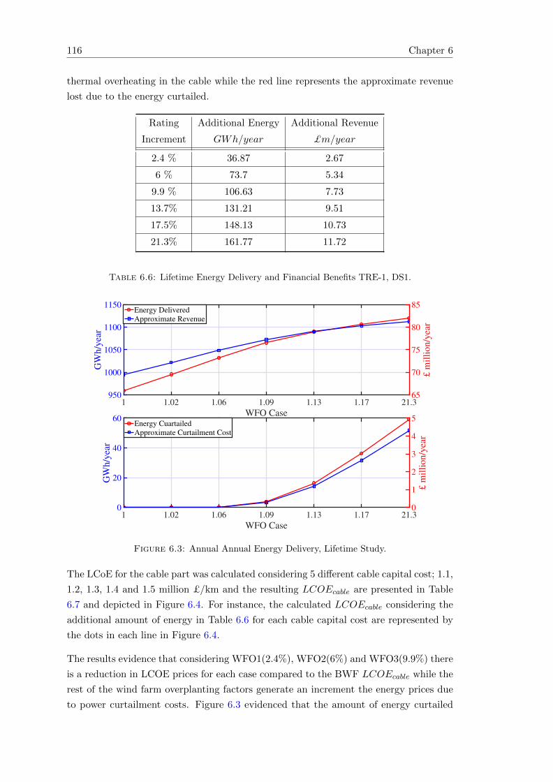
116 Chapter 6
thermal overheating in the cable while the red line represents the approximate revenue
lost due to the energy curtailed.
Rating Additional Energy Additional Revenue
Increment GWh/year £m/year
2.4 % 36.87 2.67
6 % 73.7 5.34
9.9 % 106.63 7.73
13.7% 131.21 9.51
17.5% 148.13 10.73
21.3% 161.77 11.72
Table 6.6: Lifetime Energy Delivery and Financial Benefits TRE-1, DS1.
1 1.02 1.06 1.09 1.13 1.17 21.3
WFO Case
950
1000
1050
1100
1150
GW
h/y
ear
65
70
75
80
85
£ m
illi
on/y
ear
Energy Delivered
Approximate Revenue
1 1.02 1.06 1.09 1.13 1.17 21.3
WFO Case
0
20
40
60
GW
h/y
ear
0
1
2
3
4
5£ m
illi
on/y
ear
Energy Cuartailed
Approximate Curtailment Cost
Figure 6.3: Annual Annual Energy Delivery, Lifetime Study.
The LCoE for the cable part was calculated considering 5 different cable capital cost; 1.1,
1.2, 1.3, 1.4 and 1.5 million £/km and the resulting LCOEcable are presented in Table
6.7 and depicted in Figure 6.4. For instance, the calculated LCOEcable considering the
additional amount of energy in Table 6.6 for each cable capital cost are represented by
the dots in each line in Figure 6.4.
The results evidence that considering WFO1(2.4%), WFO2(6%) and WFO3(9.9%) there
is a reduction in LCOE prices for each case compared to the BWF LCOEcable while the
rest of the wind farm overplanting factors generate an increment the energy prices due
to power curtailment costs. Figure 6.3 evidenced that the amount of energy curtailed

Economic Benefits Assessment 117
for each overplanting case studied are 0, 55MWh/year, 4GWh/year, 16 GWh/year,
36GWh/year and 59GWh/year, consequently the energy curtailment cost increase dras-
tically for WFO 4, WFO 5 and WFO 6.
Rating LCOEcable
Increment 1.1 m£/km 1.2m£/km 1.3m£/km 1.4m£/km 1.5m£/km
Base Case 4.015 4.38 4.745 5.11 5.475
2.4% 3.866 4.217 4.569 4.92 5.272
6% 3.732 4.071 4.41 4.749 5.088
9.9% 3.885 4.2143 4.542 4.871 5.199
13.7% 4.616 4.937 5.258 5.579 5.9
17.5% 5.852 6.169 6.485 6.801 7.117
21.3% 7.285 7.597 7.909 8.222 8.534
Table 6.7: LCOE Study Considering Various Cable Costs TRE-1, DS1
1 1.02 1.06 1.09 1.13 1.17 21.3
Overplanting Factor
3
4
5
6
7
8
9
LC
oE
cab
le p
art
(£/M
Wh)
£1.1 m/km
£1.2 m/km
£1.3 m/km
£1.4 m/km
£1.5 m/km
Figure 6.4: LCOE Lifetime Study.
6.3.3 Lifetime Study Concluding Remarks
The application of overplanting in the wind farm cable studied represented a finan-
cial benefit of approximately £7.73 million/year for the most favourable case found as
WFO3. A reduction between £0.13/MWh and £0.276/MWh was found for this partic-
ular overplanting scenario depending on the chosen cable capital cost.

118 Chapter 6
Additionally, the thermal risk analysis carried out across the 20 years of data demon-
strates that for WFO3 the hours ahead thermal risk estimation and curtailment mitigate
the overheating risk in 99.89% of cases while the remaining 0.11% was given by inci-
dents were the cable temperature exceeded the allowed 90C by less than 0.5C as seen
in Figure 6.2.
6.4 Cyclic Water Temperature Study TRE-1
The results in this section deal with the inclusion of variable water temperature in the
TRE studies which so far were kept constant as 15C. The addition of water temperature
(WT) variation was proposed to simulate more realistic annual cyclic conditions in the
submarine cable environment.
The investigation aims to evidence that given the variable current generation; long cable
thermal transients and; water temperature variations in the offshore cable scenario, it is
possible to safely perform rating increments without damaging the cable.
The cable system Example 1 is tested under the same WFO conditions as the ones used
in the lifetime study in Section 6.3. The online Markov Chain based TRE in Chapter
4 was tested using the year 2015 from DS2. A 6h ahead thermal risk estimation is
undertaken at every time step and an automatic preventative curtailment is applied if
any risk is estimated.
Three water temperature cycles are studied corresponding to measurements of near shore
(Location1), middle (Location2) and, far from shore (Location3) locations in the Dogger
Bank area in the North Sea at a depth of -10, -78 and -21 m respectively. The annual
water temperature cycles used are presented in Figure 6.5.
6.4.1 Thermal Risk Percentage Results
Figure 6.6 presents the obtained percentages of mitigated thermal risk after one year of
the online application of TRE-1 for the WFO scenarios considering fixed and variable
water temperature cycles. The remaining risk is not shown in the figure however it is
implied to be the remaining percentage for each case.
The results comparison evidence that the mitigated risk for the case of an overplanting
of 1.06% (WFO2) became 100% due to lower temperatures in the cable system while
WFO cases 3 and 4 registered a higher percentage of risk mitigations much more evident
for WFO4 from 95.01% to 99.8%.

Economic Benefits Assessment 119
Jan Feb Mar Apr May Jun Jul Aug Sep Oct Nov Dec
Month
4
6
8
10
12
14
16
18W
ater
Tem
per
ature
(°C
)Nearshore
Midsection
Offshore Dogger Bank
Figure 6.5: Annual Water Temperature Cycles.
10
0
10
0
10
0
10
0
98
.62 1
00
10
0
10
0
99
.63
99.8
99.8
99
.78
95
.01
99
.92
100
100
93.2
7 94.6
4
94.8
8
94
.7395
.88
95.4
95.6
9
94
.94
88
90
92
94
96
98
100
102
Fixed WT Variable WT
Location 1
Variable WT
Location 2
Variable WT
Location 3
Per
centa
ge
(%)
WF01 WFO2 WFO3 WFO4 WFO5 WFO6
Figure 6.6: Percentage of Mitigated Risk for Variable and Fixed WT cases.

120 Chapter 6
Case WFO5 and WFO6 presented almost no change (slight decrement/increment) com-
pared to the case of fixed WT due to the aggressive overload percentages that these
represent which induce a high risk of thermal overheating along the testing year.
The registered maximum conductor temperatures exceedance calculated from the re-
maining percentages was 1.4C over the 90C allowed considering the six WFO cases
studied and three offshore locations.
6.4.2 Analysis of Economic Benefits Fixed VS Variable WT
The results from the calculated annual energy delivered for the fixed and variable water
temperature cycles are summarised in Figure 6.7. The consideration of variable water
temperature along the year reduced the temperature profile of the cable allowing for
additional power delivery compared to the consideration of fixed water temperature.
Fixed WTVariable WT-
Location1
Variable WT-
Location2
Variable WT-
Location3
BWF 1021.7 1021.7 1021.7 1021.7
2.40% 1061 1061 1061 1061
6% 1099.3 1100.3 1100.3 1100.3
9.90% 1130.2 1136.1 1136.1 1136.2
13.70% 1155.2 1163.1 1163.4 1163
17.50% 1173.9 1188.1 1188.3 1186.4
21.30% 1183.1 1198.9 1203.6 1197.4
920
970
1020
1070
1120
1170
1220
GW
h/y
ear
Figure 6.7: Energy Delivery: Fixed vs Variable Water Temperature.
Case WFO1 does not induce any risk of thermal overheating, thus the amount of energy
delivered is the same for all the fixed and variable WT examples. On the other hand,
WFO2 to WFO6 induced a risk of thermal overheating thus curtailment is applied to
these cases. The amount of energy delivered considering fixed WT is less compared
to the results obtained for all the variable water temperature cases. Additionally, the
amount of energy delivered for the variable WT cases evidence that there is not a high
difference between Locations 1-3.
The optimal WFO case is selected as the most economically beneficial considering the
maximum increment in power delivery with a minimum power curtailment which will

Economic Benefits Assessment 121
allow reducing the LCOE compared to the base wind farm. Considering the case of
fixed water temperature, the optimal overplanting was WFO2 (6% load increment)
which additional power delivery represented an increment in financial benefits of approx-
imately £5.62 million/year. The calculated LCOEcable reduced between £0.2/MWh and
£0.29/MWh depending on the cable capital cost.
The optimal overplanting case considering the variable water temperature simulations
was found to be WFO3 (9.9 % load increment) with a financial benefit of approxi-
mately £8.29 million/year for the 3 offshore locations. The calculated LCOEcable was
reduced between £0.156/MWh and £0.294/MWh for Locations 1 and 2; while Location
3 presented a reduction between £0.16/MWh and £0.298/MWh considering WFO3 and
depending on the cable capital cost.
6.4.3 Cyclic Water Temperature Study Concluding Remarks
The addition of variable WT along with the developed methodology for TRE and cur-
tailment presented in Chapter 4 evidence the capacity of submarine export cables to
transfer higher ratings than the static rating limits traditionally imposed as per IEC
standards.
The amount of power delivered during one year for the BWF scenario is 1021.7 GWh/year.
By considering a modest overplanting increment of 1.02 the power delivery increases to
1099.3 GWh/year for the case of fixed WT and 1100.3 GWh/year for the case of variable
WT. The increased rating induced a 1.37 % risk of exceeding the allowed 90C (fixed
WT) and no risk for all the studied cases considering variable WT. Thus, avoiding the
need for curtailment of power generation while optimising the cable utilisation.
On the other hand, a rating increment of 6% allows to increase the annual energy
delivery to 1130.2 GWh/year (fixed WT) and 1136 GWh/year (variable WT) with a
risk of thermal overheating of 0.3656% (fixed WT) compared to an average 0.2% for the
variable WT cases. However, the calculated energy increments for WFO3 do rely on a
certain amount of power curtailment in order to avoid cable thermal overheating.
Finally, the severity of the remaining 0.2% risk of thermal overheating for WFO3 was
within 0.5C over the allowed cable temperature of 90C.
6.5 Summary
The results of the thermal risk estimation generated by the proposed algorithms com-
bined with a curtailment strategy can increase the amount of power transferred by the

122 Chapter 6
cable system while minimising the risk of exceeding the cable temperature limit. The ad-
ditional power delivered could represent an increment of energy sales and a contribution
to reducing the overall cost of energy generated offshore.
The lifetime study presented in this chapter considering DS2 and TRE-1 was able to
increase the wind farm asset by approximately £7.73 million/year for the most favourable
WFO case (WFO3) reducing the LCOEcable between £0.13/MWh and £0.276/MWh
depending on the cable capital cost.
The thermal risk analysis carried out during the 20 years of data demonstrates that for
WFO3 the mitigation of thermal overheating of overheating 99.89% while the remaining
0.11% was given by incidents where the cable temperature exceeded 90C by less than
0.5C.
The addition of variable WT in the TRE-1 methodology evidences the capacity of sub-
marine export cables to transfer higher ratings than the static rating limits traditionally
imposed as per IEC standards.On the one hand, if a modest wind farm overplanting
increment of 1.02 the power delivery increases to 1099.3 GWh/year for the case of fixed
WT and 1100.3 GWh/year for the case of variable WT.
On the other hand, if a rating increment of 6% is applied the annual energy delivery can
be increased to 1130.2 GWh/year (fixed WT) and 1136 GWh/year (variable WT) with
a risk of thermal overheating of 0.3656% (fixed WT) compared to an average 0.2% for
the variable WT cases. However, the calculated energy increments for WFO3 do rely
on a certain amount of power curtailment to avoid cable thermal overheating.
The lifetime assessment of economic benefits presented in this chapter was presented
at the 10th International Conference on Insulated Power Cables (Jicable’19) in Paris
Versailles France on June 2019 as a conference paper entitled “Assessment of financial
benefits in overplanted wind-farm export cable” [119].
Chapter 7
Conclusion
Submarine power cables are traditionally sized considering static rating calculations as
is traditionally done with cables on land however offshore cables, face variable power
generation with short periods of full power generations which due to large cable thermal
time constants underutilise the cable capacity.
The alternative real-time rating methodologies and estimation methods in the literature
have been mostly developed for cables installed on land and do not consider the highly
variable load profile or uncertainty in the hours ahead power generation thus, they can
not be directly applied in submarine cables.
The research in this thesis contributes to the above gap in the literature with the de-
velopment of a series of algorithms based on the use of probabilistic methods such as
Monte Carlo Simulation, Markov Chain Theory and load power ramp event character-
isation which are able to estimate forward thermal risk in offshore wind farm cables
under overplanting scenarios.
The developed algorithms make use of a limited amount of historical data to extract
information such as seasonal trends and patterns of power generation thus represent-
ing a cost-effective methodology able to perform hours ahead thermal risk estimations
considering data collected from initial surveys in offshore sites represent a big advantage.
The algorithms proved to generate a high percentage of accurate estimation of thermal
risk up to 6h ahead and can be used as an offline/online decision-making tool. The
offline simulation study can be used during planning stages of wind farm projects for
cable optimization while the online tool can help the system operation to maximise the
power delivered through the cable system while avoiding the risk of thermal overheating
in the cable.
Finally, the online application of the developed methods along with a power curtailment
strategy was able to increase in the amount of electric power transferred from offshore
123

124 Chapter 7
wind farm installations by estimating and mitigating the likelihood of the cable exceeding
its temperature limit of 90C. The optimisation of cable capacity while guarding against
thermal damage in the cable was achieved thus fulfilling the main objective for this thesis.
7.1 Research Summary
The developed probabilistic methodologies can generate a quantitative risk of temper-
ature exceedance for the case of offshore wind farm cables. The novel algorithms can
be used as an online/offline decision-making tool that could contribute towards the de-
velopment and application of non-static rating methodologies in submarine cables to
optimise the cable installation capacity.
Chapter 3 presents the development of a probabilistic algorithm based on a Monte Carlo
Analysis of monthly probability distributions of load current that can estimate likely risk
of cable overheating in as much as 98% of the estimations performed in one year for a
6 hours ahead estimation window. The methodology accuracy over a 6h, 12h and 24h
ahead estimation window and three different lengths of training data set between 5 and
19 years of data were studied.
The work in Chapter 3 led to the selection of the 6h window as the most accurate
while still giving enough time for planning and performing curtailment in an offshore
installation. Additionally, the use of 5 years of data for the statistical analysis was
proved to be enough to perform accurate estimations which given the limited amount
of historical data from offshore locations represent a big advantage.
Chapter 4 introduced a Markov Chain model for the optimisation of the load sampling
strategy used by the pure MCS algorithm in Chapter 3. The evaluation of 6 Markov
Chain models with a different number of system states (4, 8 and 17) and 1st and 3rd
order TPM were developed and tested.
The TPMs are built from the monthly analysis of 5 years of data which extracts the
historical transition between the states. The transition probability from the load current
going from the current state to a different state is calculated at each time step in the
analysis and use to estimate likely load current scenarios correlated to the actual state
of the system. This approach was able to generate a reduction in misclassification cases
compared to the MCS based algorithm as presented in Section 4.6.
The Markov Chain based methodology proved to generate a high percentage of positive
identifications of risk 6h ahead from 95.68% in WFO3 to 98.09% in WFO1 during one
year of offline testing with an MAE of 0.0158 and 0.0419 respectively. The online appli-
cation of the methodology including a simulated curtailment strategy generated a high
percentage of thermal risk mitigation while the analysis of the percentage of remaining

Conclusion 125
thermal exceedances did not exceed a temperature higher than 91.5C for DS1 and 91C
for DS2.
The calculated additional power compared to the traditional limiting rating based on
IEC60287 (1149.58 GWh/year) was 7.26%, 9.16% and 9.67% per year with an approx-
imate revenue of 6.05, 7.63 and 8.06 million £/year for DS1. Tests performed in two
datasets from different offshore locations proved that the statistically-based method is
easy to use, non-restrictive or parametric to a specific set of data.
Chapter 5 proposed an alternative methodology based on load current ramp identifica-
tion technique where the main objective is focused on the early identification of ramp
direction and intensity which combined with a historical analysis of ramp events, esti-
mate the hours ahead thermal risk in the cable according to the initial ramp rate.
A statistical analysis of historical data is used to extract ramp rate characteristics from
the studied dataset to identify ramps, estimate future load current scenarios and, likely
cable temperatures. The estimated conductor temperatures are used to calculate and
prevent the risk of temperature exceedance in the export cable while the application of
overplanting scenarios allows the optimisation of transmission capacity.
The example studied in Chapter 4 was limited to the submarine section of the cable
system while the example cable system in Chapter 5 performs an extended analysis
considering also the landfall section of the cable which is known to present thermally
limiting characteristics. The results of the simulated overplanting cases shown an addi-
tional power delivery of up to 15.3% per year compared to the application of traditional
static ratings based on IEC60287. The comparison with the results in Chapter 4 show
improvement of more than 50% for the false-positive identifications of risk, which rep-
resented a reduction of the financial benefits for the system.
An economic assessment of financial benefits analysis is presented in chapter 6 showing
how the online application of the developed TRE tools in Chapters 4 and 5 can generate
additional power delivery and contribute to reducing the LCOE of the wind farm. The
consideration of variable water temperature along the year reduced the temperature
profile of the cable allowing for additional power delivery compared to the consideration
of fixed water temperature.
7.1.1 Key Remarks
A key difference between the methodologies presented in Chapter 4 and Chapter 5 is the
ability of the former to be applied to different wind farm projects without modifications
due to the use of the non-parametric Markov Chain based method which can generate
TPM only relying on the input load current data from the offshore site.

126 Chapter 7
On the other hand, the latter approach is focused solely on the study of fast power
variations in the historical load current data. Thus, the algorithm parameters and ramp
rate classification cases are case dependent and are not easy to generalise due to their
underlying meteorological and geographical nature.
The developed methodologies can be applied to wind farm cable systems where wind
farm overplanting is applied for economic benefits. The algorithms would help to increase
the power delivery by avoiding unnecessary power curtailment when the cable rating is
higher than the static rating but the cable temperature is low. Furthermore, the online
application tool could be a particularly useful backup for cable monitoring if the DTS
technology is not available or installed.
The wind farm overplanting cases studied in this thesis can be adjusted as needed by
the user depending on the wind farm and cable studied and the required amount of data
of the offshore site is just 5 years which could be obtained in early stages of wind farm
projects. Additionally, the method could be applied to different wind farm locations and
cable sizes given the necessary data from the site and can represent additional financial
benefits even for a small wind farm size as the one analysed in the study.
Thermally limiting locations across the cable route can be the point of study as the
soil parameters and burial depth are easily changed in the cable model. Additionally,
a study of k thermal sections in the cable can be carried out to account for different
environmental conditions across the cable line.
Finally, the cable model used in the study is not an extension of the proposed method-
ology thus the method can work with any thermal model and specific cable system that
the user may have. The cable system, thermal model and ambient parameters can be
adapted to suit specific conditions, for instance, a variable temperature profile could be
added into the framework as presented in Chapter 6.
7.2 Guidelines for Future Work
Despite the contribution made by this thesis, several areas have been identified which
merit further work. For instance, the inclusion of variable ambient parameters such as
soil thermal resistivity though out the cable route could be tested as a parallel analysis
to have an extended reference of thermal estimations along the line.
The years of separation between training and testing data demonstrate that data gath-
ered from initial surveys can represent monthly/annual patterns from the offshore lo-
cation in a long-time span ahead. Thus, given sufficient input, the algorithm could be
trusted even when a data update cannot be performed immediately. However, it has
been suggested to reduce the gap between the years of training and testing to quantify
the impact that this action may induce in the results.

Conclusion 127
The validation of the developed tool could benefit from the study of an existing opera-
tional wind farm project, given the necessary data, to include specific parameters such as
cable charging current, wind park wake effect losses, wind farm availability percentages
and array cable losses. These considerations would likely reduce the wind power yield
which may further increase the room for additional power delivery while minimising the
thermal risk in the cable system.
Additionally, as mentioned earlier the application of the methodology in Chapter 5 relies
on the selection of case dependent parameters given the available data set, thus further
analysis and experiments considering a second data, as done for the Markov Chain
methodology in Chapter 4, could further validate the obtained results.
Finally, the calculation of the LCOE for the cable part was a simple financial analysis
which is much more complex in real life thus, if the developed methodologies are applied
to the study of an existing wind farm project the cable losses as well as infrastruc-
tural investments, operation/maintenance expenditures and a lower energy sale price in
accordance with the recent reduction in energy prices could be performed.


Appendix A
Finite Difference Model
The submarine cable thermal network of a typical 3 core submarine cable construction
was presented in Figure 3.10 along with the corresponding set of parameters, see Section
3.4.
The set of partial differential equations obtained from the cable circuit for the calculation
of cable temperatures at nodes θc, θs, θj , θa, θo, θe where the subscripts c, i, s, j, f , b,
a, o and e correspond to conductor, insulation, sheath, jacket, filler, bedding, armour,
outer covering and external environment are shown below
d
dtθc(C1 + C2) = W1 −
(θc − θs)T1
d
dtθs(C3 + C4 + C5) = Ws+
(θc − θs)T1
− (θs − θj)T2a
d
dtθj(C6 + C7 + C8) =
(θs − θj)T2b
− (θj − θa)
T2ad
dtθa(C9 + C10 + C11) =
(θj − θa)
T2a+W3 −
(θa − θo)T3
d
dtθoC12 =
(θa − θo)T3
− (θo − θe)T4a
d
dtθeC13 =
(θo − θe)T4a
− (θe − θamb)
T4b
(A.1)
The system of linear equations A ∗ x = B shown below is solved for x at each time step
in the developed TRE methodologies in order to obtain the temperatures at each node
of the cable considering changes in load data.
129
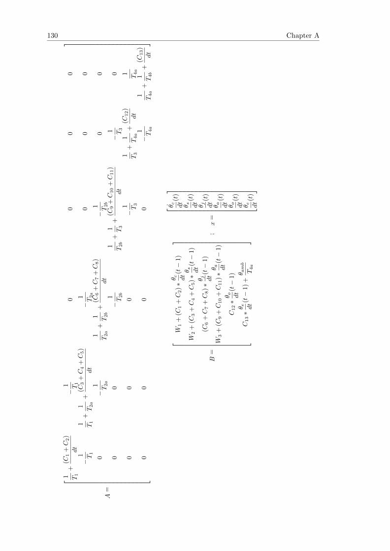
130 Chapter A
A=
1 T1
+(C
1+C
2)
dt
−1 T1
00
00
−1 T1
1 T1
+1 T2a
+(C
3+C
4+C
5)
dt
−1 T2a
00
0
0−
1 T2a
1 T2a
+1 T2b
+(C
6+C
7+C
8)
dt
−1 T2b
00
00
−1 T2b
1 T2b
+1 T3
+(C
9+C
10
+C
11)
dt
−1 T3
0
00
0−
1 T3
1 T3
+1 T4a
+(C
12)
dt
1 T4a
00
00
−1 T4a
1 T4a
+1 T4b
+(C
13)
dt
B=
W1
+(C
1+C
2)∗θ c dt(t−
1)
W2
+(C
3+C
4+C
5)∗θ s dt(t−
1)
(C6
+C
7+C
8)∗θ j dt(t−
1)
W3
+(C
9+C
10
+C
11)∗θ a dt(t−
1)
C12∗θ o dt(t−
1)
C13∗θ e dt(t−
1)
+θ a
mb
T4a
;x
=
θ c dt(t
)
θ s dt(t
)
θ j dt(t
)
θ a dt(t
)
θ o dt(t
)
θ e dt(t
)

Appendix B
List of Published Papers
B.1 Refereed Conference Papers
The following papers have been presented at International Conferences and have been
subject to peer review, the papers are listed in chronological order.
Hernandez-Colin M.A., Pilgrim J.A., “Offshore Cable Optimisation by Probabilistic
Thermal Risk Estimation”, International Conference on Probabilistic Methods Applied
to Power Systems (PMAPS 2018), Idaho,United States, June 2018, pp.1-6. URL.
Hernandez-Colin M.A., Pilgrim J.A.,“On-line Markov Chain Based Thermal Risk Esti-
mation for Offshore Wind Farm Cables”, 17th International Workshop on Large Scale
Integration of Wind Power into Power Systems as well as on Transmission Networks for
Offshore Wind Farms, Stockholm, Sweden, October 2018, pp.1-6. URL.
Hernandez-Colin M.A., Pilgrim J.A.,“Assessment of financial benefits in over-planted
wind-farm export cable”, 10th International Conference on Insulated Power Cables (Ji-
cable’19), Paris Versailles France, June 2019, pp.1-6. URL.
B.2 Peer Reviewed Journal Papers
The paper below have been accepted for publication in a peer reviewed academic journal.
Hernandez-Colin M.A., Pilgrim J.A.,“Cable Thermal Risk Estimation for Over-planted
Wind Farms”, IEEE Transactions on Power Delivery, Accepted May 2019, In press,
pp.1-9. URL.
The following paper is awaiting decisions at the point of submission of the thesis:
131

132 Chapter B
Hernandez-Colin M.A., Pilgrim J.A.,“Improving Export Cable Thermal Risk Manage-
ment via Ramp Identification”, IEEE Transactions on Power Delivery, Submitted: Oc-
tober 4th 2019, pp.1-9.
Bibliography
[1] J. A. Pilgrim and S. Kelly, “Thermal and economic optimisation of windfarm
export cable,” IET Renewable Power Generation 2018, pp. 1–6, 2018.
[2] M. Ardelean and P. Minnebo, “HVDC Submarine Power Cables in
the World,” tech. rep., Joint Research Centre, 2015. [Online]. Avail-
able https://publications.jrc.ec.europa.eu/repository/bitstream/JRC97720/ld-na-
27527-en-n.pdf [Accessed:09-Jun-2019].
[3] C. Ensen, T. Kvarts, P. Cavaleiro, L. R. Casals, E. Guix, G. Dell’anna, W. Fre-
lin, H. Heo, F. Lesur, B. Mampaey, S. Meijer, E. Olsen, P. O’rourke, H. Or-
ton, R. Wilson, T. Worzyk, R. D. Zhang, C. Ensen, T. Kvarts, P. Cavaleiro,
L. R. Casals, E. Guix, G. Dell’anna, W. Frelin, H. Heo, F. Lesur, B. Mampaey,
S. Meijer, E. Olsen, P. O’rourke, H. Orton, R. Wilson, T. Worzyk, R. D. Zhang,
X. Feng, O. Matsunaga, C. Jensen, T. Kvarts, P. Cavaleiro, L. R. Casals, E. Guix,
G. Dell’anna, W. Frelin, H. Heo, F. Lesur, B. Mampaey, S. Meijer, E. Olsen,
P. Orourke, H. Orton, R. Wilson, T. Worzyk, and R. D. Zhang, “Offshore Gener-
ation Cable Connections, Working Group B1.40,” International Council on Large
Electric Systems (Cigre), no. 610, pp. 1–180, 2015.
[4] ABB, “XLPE Submarine Cable Systems Attachment to
XLPE Land Cable Systems-Users Guide,” tech. rep., 2010.
[Online].Available:https://new.abb.com/docs/default-source/ewea-doc/xlpe-
submarine-cable-systems-2gm5007.pdf. [Accessed: 28-Aug-2018].
[5] N. Hampton, R. Hartlein, H. Lennartsson, H. Orton, and R. Ramachandran,
“Long-Life Xlpe Insulated Power Cable,” in 7th International Conference on In-
sulated Power Cable (Jicable), pp. 1–6, 2007.
[6] I. E. C. IEC, “IEC 60287-1: Electric cables–Calculation of the current rating, Part
1: Current rating equations (100% load factor) and calculation of losses-General.,”
2014.
[7] S. P. Walldorf, S. John, and F. J. Hoppe, “The Use of Real-Time Monitoring
and Dynamic Ratings for Power Delivery Systems and Implication for Dielectric
Materials,” IEEE Electrical Insulation Magazine, pp. 28–33, 1999.
133

134
[8] J. K. Dix, T. J. Hughes, C. J. Emeana, J. A. Pilgrim, T. J. Henstock, T. M.
Gernon, and C. E. L. Thompson, “Substrate controls on the life-time performance
of marine HV cables,” in Smarter Solutions for Future Off shore Developments,
pp. 88–107, 2017.
[9] S. Catmull, R. Chippendale, J. Pilgrim, G. Hutton, and P. Cangy, “Cyclic Load
Profiles for Offshore Wind Farm Cable Rating,” IEEE Transactions on Power
Delivery, vol. 31, no. 3, pp. 1242–1250, 2016.
[10] C. Wolter, H. Klinge Jacobsen, G. Rogdakis, L. Zeni, and N. A. Cutululis, “Over-
planting in offshore wind power plants in different regulatory regimes,” in 15th
wind Integration workshop - International Workshop on Large-Scale Integration of
Wind Power into Power Systems as well as on Transmission Networks for Offshore
Wind Power Plants, pp. 1–8, 2016.
[11] S. M. Foty, G. J. Anders, and S. J. Croall, “Cable environment analysis and the
probabilistic approach to cable rating,” IEEE Transactions on Power Delivery,
vol. 5, no. 3, pp. 1628–1633, 1990.
[12] G. Idicula and E. Davies, “The probabilistic rating of separate pipe cooled cables,”
in 3rd International Conference on Probabilistic Methods Applied to Power Systems
(PMAPS), pp. 185–190, 1991.
[13] A. K. Blackwell, Forecasting and probabilistic rating of underground power cables.
Doctorate of philosophy dissertation, University of Southampton, 1996.
[14] X. Zhou, Y. Tang, Y. Xie, Y. Li, and H. Zhang, “A Fuzzy Probability-based
Markov Chain Model for Electric Power Demand Forecasting of Beijing, China,”
Energy and Power Engineering, vol. 5, pp. 488–492, 2013.
[15] J. Staats and C. Bruce-boye, “Markov Chain based Very Short-Term Load
Forecasting realizing Conditional Expectation,” in International ETG Congress,
(Bonn, Germany), pp. 254–259, 2017.
[16] M. K. Haider, A. K. Ismail, and I. A. Qazi, “Markovian models for electrical load
prediction in smart buildings,” in International Conference on Newral Information
Processing, pp. 632–639, 2012.
[17] C. Gallego-Castillo, A. Cuerva-Tejero, and O. Lopez-Garcia, “A review on the
recent history of wind power ramp forecasting,” Renewable and Sustainable Energy
Reviews, vol. 52, pp. 1148–1157, 2015.
[18] T. Worzyk, Submarine Power Cables, Design, Installation, Repair, Environmental
Aspects. Springer-Verlag Berlin Heidelberg, 1 ed., 2009.
[19] G. J. Anders, Rating of Electric Power Cables, Ampacity computatin for trans-
mission, distribution, and industrial applications. IEEE Press, 1997.

Bibliography 135
[20] A. Ukil, H. Braendle, and P. Krippner, “Distributed temperature sensing: Review
of technology and applications,” IEEE Sensors Journal, vol. 12, no. 5, pp. 885–892,
2012.
[21] Y. C. Liang and Y. M. Li, “On-line dynamic cable rating for underground cables
based on DTS and FEM,” WSEAS Transactions on Circuits and Systems, vol. 7,
no. 4, pp. 229–238, 2008.
[22] H. J. Li, K. C. Tan, and Q. Su, “Assessment of underground cable ratings based on
distributed temperature sensing,” IEEE Transactions on Power Delivery, vol. 21,
no. 4, pp. 1763–1769, 2006.
[23] M. Olschewski, W. Hill, and L. T. Gmbh, “Performance Optimization of Under-
ground Power Cables using Real-Time Thermal Rating,” International Conference
on Insulated Power Cable (Jicable), pp. 4–7, 2015.
[24] I. E. C. IEC, “IEC 602853-2: Calculation of the cyclic and emergency current
rating of cables, Part 2: Cyclic rating of cables greater than 18/30 (36) kV and
emergency ratings for cables of all voltages,” 1989.
[25] D. Chatzipetros and J. Pilgrim, “Impact of Proximity Effects on Sheath Losses
in Trefoil Cable Arrangements,” IEEE Transactions on Power Delivery, pp. 1–9,
2019.
[26] J. A. Pilgrim, S. Catmull, R. Chippendale, P. L. Lewin, P. Stratford, and R. Tyre-
man, “Current Rating Optimisation for Offshore Wind Farm Export Cables,” in
International Council on Large Electric Systems (Cigre), pp. 1–7, 2014.
[27] S. Sturm and J. Paulus, “Estimating the losses in three-core submarine power ca-
bles using 2D and 3D FEA simulations,” 9th International Conference on Insulated
Power Cables, pp. 21–25, 2015.
[28] R. Edf, D. France, P. Sauvage, E. D. F. C. France, C. Moreau, R. Edf, D. France,
N. Boudinet, R. T. E. C. France, G. D. E. Robien, and E. D. F. C. France, “Ar-
mour loss measurements in three-core medium voltage cables: comparison with iec
standards and fem calculations,” in 23rd International Conference on Electricity
Distribution, (Lyon), pp. 1–5, 2015.
[29] M. M. Hatlo and J. J. Bremnes, “Current dependent armour loss in three-core
cables: Comparison of FEA results and measurements,” International Council on
Large Electric Systems (Cigre), no. 1, pp. 1–8, 2014.
[30] J. H. Neher and M. H. McGrath, “The Calculation or the Temperature Rise
and Load Capability of Cable Systems,” Transactions of the American Institute
of Electrical Engineers. Part III: Power Apparatus and Systems, vol. 76, no. 3,
pp. 752–764, 1957.

136
[31] J. H. Neher, “The Transient Temperature Rise of Buried Cable Systems,” IEEE
Transactions on Power Apparatus and Systems, vol. 83, no. 2, pp. 102–114, 1964.
[32] I. E. C. IEC, “IEC 60287-2: Electric cables–Calculation of the current rating, Part
2: Thermal Resistance, calculation of the thermal resistance.,” 2015.
[33] K. F. Goddard, J. A. Pilgrim, R. Chippendale, and P. L. Lewin, “Induced losses
in three-core SL-type high-voltage cables,” IEEE Transactions on Power Delivery,
vol. 30, no. 3, pp. 1505–1513, 2015.
[34] G. Anders and G. Georgallis, “Transient analysis of 3-core SL-type submarine
cables with jacket around each core,” International Conference on Insulated Power
Cable (Jicable), pp. 1–6, 2015.
[35] R. Huang, J. A. Pilgrim, P. L. Lewin, D. Scott, and D. Morrice, “Managing cable
thermal stress through predictive ratings,” in 33rd Electrical Insulation Confer-
ence, no. June, pp. 110–113, 2015.
[36] J. A. Pilgrim, D. J. Swaffield, P. L. Lewin, and D. Payne, “An investigation
of thermal ratings for high voltage cable joints through the use of 2D and 3D
Finite Element Analysis,” Conference Record of IEEE International Symposium
on Electrical Insulation, pp. 543–546, 2008.
[37] R. D. Chippendale, J. A. Pilgrim, K. F. Goddard, and P. Cangy, “Analytical
thermal rating method for cables installed in J-Tubes,” IEEE Transactions on
Power Delivery, vol. 32, no. 4, pp. 1721–1729, 2017.
[38] J. A. Pilgrim, P. L. Lewin, S. T. Larsen, F. Waite, and D. Payne, “Rating of cables
in unfilled surface troughs,” IEEE Transactions on Power Delivery, vol. 27, no. 2,
pp. 993–1001, 2012.
[39] D. Swaffield, P. Lewin, and S. Sutton, “Methods for rating directly buried high
voltage cable circuits,” IET Generation, Transmission & Distribution, vol. 2, no. 3,
pp. 393–401, 2008.
[40] F. de Leon and G. J. Anders, “Effects of backfilling on cable ampacity analyzed
with the finite element method,” IEEE Transactions on Power Delivery, vol. 23,
no. 2, pp. 537–543, 2008.
[41] R. S. Olsen, J. Holboll, and U. S. Gudmundsdottir, “Dynamic temperature esti-
mation and real time emergency rating of transmission cables,” IEEE Power and
Energy Society General Meeting, pp. 1–8, 2012.
[42] M. Diaz-Aguilo and F. de Leon, “Introducing Mutual Heating Effects in the
Ladder-Type Soil Model for the Dynamic Thermal Rating ofUnderground Ca-
bles,” IET Science, Measurement & Technology, vol. 30, no. 4, pp. 1958–1964,
2015.

Bibliography 137
[43] S. Dubitsky, G. Greshnyakov, and N. Korovkin, “Comparison of finite element
analysis to IEC-60287 for predicting underground cable ampacity,” in IEEE In-
ternational Energy Conference, pp. 1–6, 2016.
[44] P. Lewin, D. Swaffield, S. Larsen, and D. Payne, “Effects of modelling assumptions
on the rating calculation for externally forced cooled high-voltage cables,” IET
Generation Transmission & Distribution, vol. 3, no. 5, pp. 496–507, 2009.
[45] E. Fernandez, I. Albizu, M. Bedialauneta, A. Mazon, and P. Leite, “Dynamic line
rating systems for wind power integration,” in IEEE PES PowerAfrica, pp. 1–7,
2012.
[46] G. Anders, A. Napieralski, S. Zubert, and M. Orlikowski, “Advanced modeling
techniques for dynamic feeder rating systems,” IEEE Transactions on Industry
Applications, vol. 2, no. 3, pp. 1012–1019, 2002.
[47] F. D. Leon, “Calculation of Underground Cable Ampacity,” in CYME Interna-
tional T&D, pp. 1–6, 2005.
[48] D. A. Douglass and A. A. Edris, “Real-time monitoring and dynamic thermal
rating of power transmission circuits,” IEEE Transactions on Power Delivery,
vol. 11, no. 3, pp. 1407–1415, 1996.
[49] S. H. Huang, W. J. Lee, and M. T. Kuo, “An online dynamic cable rating system for
an industrial power plant in the restructured electric market,” IEEE Transactions
on Industry Applications, vol. 43, no. 6, pp. 1449–1458, 2007.
[50] R. Olsen, J. Holboell, and U. S. Gudmundsdottir, “Electrothermal coordination
in cable based transmission grids,” IEEE Transactions on Power Systems, vol. 28,
no. 4, pp. 4867–4874, 2013.
[51] H. Brakelmann, H. Hirsch, A. Rohrich, H.-p. Scheiffarth, and J. Stammen, “Adap-
tive monitoring program for dynamic thermal rating,” in International Conference
on Insulated Power Cable (Jicable), pp. 1–5, 2007.
[52] M. Diaz-Aguilo, F. de Leon, S. Jazebi, and M. Terracciano, “Ladder-Type Soil
Model for Dynamic Thermal Rating of Underground Power Cables,” IEEE Power
and Energy Technology Systems Journal, vol. 1, pp. 21–30, 2014.
[53] M. Diaz-Aguilo and F. de Leon, “Adaptive soil model for real-time thermal rating
of underground power cables,” IET Science, Measurement & Technology, vol. 9,
no. 6, pp. 654–660, 2014.
[54] Y. Yan, W. Zhang, H. Lin, Z. Li, and R. Tang, “Field validation of a weather-
based dynamic rating system for transmission lines,” in IEEE Innovative Smart
Grid Technologies - Asia, 2016.
138
[55] S. C. Jupe, D. Kadar, G. Murphy, M. G. Bartlett, and K. T. Jackson, “Application
of a dynamic thermal rating system to a 132kV distribution network,” in IEEE
PES Innovative Smart Grid Technologies Conference Europe, pp. 1–8, 2011.
[56] A. H. Wijethunga, J. V. Wijayakulasooriya, J. B. Ekanayake, and N. D. Silva,
“Conductor temperature based low cost solution for dynamic line rating calcula-
tion of power distribution lines,” IEEE 10th International Conference on Industrial
and Information Systems, pp. 128–133, 2015.
[57] C. R. Black and W. A. Chisholm, “Key Considerations for the Selection of Dy-
namic Thermal Line Rating Systems,” IEEE Transactions on Power Delivery,
vol. 30, no. 5, pp. 2154–2162, 2015.
[58] A. Michiorri and P. C. Taylor, “Forecasting real-time ratings for electricity dis-
tribution networks using weather forecast data,” in 20th International Conference
on Electricity Distribution CIRED, pp. 1–4, 2009.
[59] M. El-Kady, F. Chu, H. Radhakrishna, D. Horrocks, and R. Ganton, “A proba-
bilistic approach to power cable thermal analysis and ampacity calculation,” IEEE
Transactions on Power Apparatus and Systems, vol. 103, no. 9, pp. 2735–2740,
1984.
[60] A. K. Blackwell, A. E. Davies, and C. Ong-Hall, “Forecasting Cable Ratlngs Uslng
a Probabilistic Method and Real Time Parameter,” in Sixth International Confer-
ence on AC and DC Power Transmission, no. 423, pp. 81–85, 1996.
[61] J. Zhang, J. Pu, J. D. McCalley, H. Stern, and W. A. Gallus, “A Bayesian ap-
proach for short-term transmission line thermal overload risk assessment,” IEEE
Transactions on Power Delivery, vol. 17, no. 3, pp. 770–778, 2002.
[62] D. M. Kim, J. M. Cho, H. S. Lee, H. S. Jung, and J. O. Kim, “Prediction of
dynamic line rating based on assessment risk by time series weather model,”
9th International Conference on Probabilistic Methods Applied to Power Systems
(PMAPS), pp. 1–7, 2006.
[63] D. J. Morrow, J. Fu, and S. M. Abdelkader, “Experimentally validated partial
least squares model for dynamic line rating,” IET Renewable Power Generation,
vol. 8, no. 3, pp. 260–268, 2014.
[64] R. Huang, J. A. Pilgrim, P. L. Lewin, D. Scott, and D. Morrice, “Cable Tunnel
Thermal Rating Prediction using Support Vector Regression,” in International
Conference on Probabilistic Methods Applied to Power Systems (PMAPS), pp. 1–
6, 2014.
[65] Z. Wei, M. Wang, X. Han, H. Zhang, and Q. Zhang, “Probabilistic forecasting for
the ampacity of overhead transmission lines using quantile regression method,”

Bibliography 139
in Asia-Pacific Power and Energy Engineering Conference, pp. 1632–1635, IEEE,
2016.
[66] R. Dupin, A. Michiorri, and G. Kariniotakis, “Dynamic line rating day-ahead fore-
casts cost benefit based selection of the optimal quantile,” in CIRED Workshop,
(Helsinki, Finland), pp. 1–4, 2016.
[67] J. Fu, D. J. Morrow, and S. M. Abdelkader, “Modelling and prediction techniques
for dynamic overhead line rating,” IEEE Power and Energy Society General Meet-
ing, pp. 1–7, 2012.
[68] Q. Li, M. Musavi, and D. Chamberlain, “Overhead conductor thermal rating us-
ing neural networks,” IEEE International Conference on Smart Measurements for
Grids, Proceedings, pp. 139–142, 2011.
[69] H. Shaker, M. Fotuhi-Firuzabad, and F. Aminifar, “Fuzzy dynamic thermal rat-
ing of transmission lines,” IEEE Transactions on Power Delivery, vol. 27, no. 4,
pp. 1885–1892, 2012.
[70] X. Liang and L. Goel, “Distribution system reliability evaluation using the Monte
Carlo simulation method,” Electric Power Systems Research, vol. 40, no. 2, pp. 75–
83, 1997.
[71] L. Zhao, T. Mao, W. Xu, J. Luan, J. Wu, and G. Qi, “A Review of Risk Assessment
Methods for Power System,” MATEC Web of Conferences, vol. 139, pp. 1–6, 2017.
[72] K. J. Timko, A. Bose, and P. M. Anderson, “Monte Carlo Simulation of Power
System Stability,” IEEE Transactions on Power Apparatus and Systems, vol. 102,
no. 10, pp. 3453–3459, 1983.
[73] T. Ringelband, P. Schafer, and A. Moser, “Probabilistic ampacity forecasting for
overhead lines using weather forecast ensembles,” Electrical Engineering, vol. 95,
no. 2, pp. 99–107, 2013.
[74] A. Michiorri, P. C. Taylor, and S. C. Jupe, “Overhead line real-time rating es-
timation algorithm: Description and validation,” Proceedings of the Institution
of Mechanical Engineers, Part A: Journal of Power and Energy, vol. 224, no. 3,
pp. 293–304, 2010.
[75] A. Carpinone, M. Giorgio, R. Langella, and A. Testa, “Markov chain modeling
for very-short-term wind power forecasting,” Electric Power Systems Research,
vol. 122, pp. 152–158, 2015.
[76] C. Miao, J. Chen, J. Liu, and H. Su, “An Improved Markov Chain Model for
Hour-Ahead Wind Speed Prediction,” in 34th Chinese Control Conference, no. 2,
pp. 8252–8257, 2015.

140
[77] M. He, L. Yang, J. Zhang, and V. Vittal, “A spatio-temporal analysis approach
for short-term forecast of wind farm generation,” IEEE Transactions on Power
Systems, vol. 29, no. 4, pp. 1611–1622, 2014.
[78] L. Yang, M. He, J. Zhang, and V. Vittal, “Support-vector-machine-enhanced
markov model for short-term wind power forecast,” IEEE Transactions on Sus-
tainable Energy, vol. 6, no. 3, pp. 791–799, 2015.
[79] Y. Li and J. Niu, “Forecast of power generation for grid-connected photovoltaic
system based on Markov chain,” in Asia-Pacific Power and Energy Engineering
Conference, pp. 9–12, 2009.
[80] I. Sanchez, “Short-term prediction of wind energy production,” International Jour-
nal of Forecasting, vol. 22, no. 1, pp. 43–56, 2006.
[81] M. G. Lobo and I. Sanchez, “Regional wind power forecasting based on smoothing
techniques, with application to the Spanish peninsular system,” IEEE Transac-
tions on Power Systems, vol. 27, no. 4, pp. 1990–1997, 2012.
[82] G. Papaefthymiou and B. Klockl, “MCMC for wind power simulation,” IEEE
Transactions on Energy Conversion, vol. 23, no. 1, pp. 234–240, 2008.
[83] T. Pesch, S. Schroders, H. J. Allelein, and J. F. Hake, “A new Markov-chain-
related statistical approach for modelling synthetic wind power time series,” New
Journal of Physics, vol. 17, 2015.
[84] P. Pinson and H. Madsen, “Adaptive modelling and forecasting of offshore wind
power fluctuations with Markov-switching autoregressive models,” Journal of
Forecasting, vol. 31, no. 4, pp. 281–313, 2012.
[85] S. Balluff, J. Bendfeld, and S. Krauter, “Short term wind and energy prediction
for offshore wind farms using neural networks,” International Conference on Re-
newable Energy Research and Applications, vol. 5, pp. 379–382, 2015.
[86] D. R. Chandra, M. S. Kumari, and M. Sydulu, “A detailed literature review on
wind forecasting,” in International Conference on Power, Energy and Control,
pp. 630–634, 2013.
[87] S. S. Soman, H. Zareipour, O. Malik, and P. Mandal, “A review of wind power
and wind speed forecasting methods with different time horizons,” North American
Power Symposium (NAPS), pp. 1–8, 2010.
[88] G. Kariniotakis, D. Mayer, J. Moussafir, R. Chevallaz-Perrier, J. Usaola,
I. Sanchez, I. Marti, H. Madsen, T. S. Nielsen, C. Lac, P. Frayssinet, H. Waldl,
J. Halliday, G. Giebel, G. Kallos, J. Ottavi, U. Focken, M. Lange, D. Heinemann,
J. K. Ancin, J. Toefting, P. O’Donnel, D. M. Coy, M. Collmann, A. Gigandidou,
G. Gonzales-Morales, C. Barquero, I. Cruz, and N. D. Hatziargyriou, “Anemos :

Bibliography 141
development of a next generation wind power forecasting system for the large-scale
integration of onshore & offshore wind farms,” Ewec 2003, pp. 1–5, 2003.
[89] X. Wang, P. Guo, and X. Huang, “A review of wind power forecasting models,”
Energy Procedia, vol. 12, pp. 770–778, 2011.
[90] J. Yan, K. Li, S. Member, and E.-w. Bai, “Hybrid Probabilistic Wind Power
Forecasting Using Temporally Local Gaussian Process,” vol. 7, pp. 87–95, 2016.
[91] E. Mangalova and E. Agafonov, “Wind power forecasting using the k-nearest
neighbors algorithm,” International Journal of Forecasting, vol. 30, no. 2, pp. 402–
406, 2014.
[92] A. M. Foley, P. G. Leahy, A. Marvuglia, and E. J. McKeogh, “Current methods
and advances in forecasting of wind power generation,” Renewable Energy, vol. 37,
no. 1, pp. 1–8, 2012.
[93] J. Jung and R. P. Broadwater, “Current status and future advances for wind
speed and power forecasting,” Renewable and Sustainable Energy Reviews, vol. 31,
pp. 762–777, 2014.
[94] R. Perveen, N. Kishor, and S. R. Mohanty, “Offshore wind farm develop-
ment: Present status and challenges,” Renewable and Sustainable Energy Reviews,
vol. 29, pp. 780–792, 2014.
[95] A. K. Nayak, K. C. Sharma, R. Bhakar, and J. Mathur, “ARIMA based statistical
approach to predict wind power ramps,” IEEE Power and Energy Society General
Meeting, vol. 2015-Septe, pp. 1–5, 2015.
[96] R. Sevlian and R. Rajagopal, “Detection and statistics of wind power ramps,”
IEEE Transactions on Power Systems, vol. 28, no. 4, pp. 3610–3620, 2013.
[97] Huan Ma and Yutian Liu, “Real-time recognition of wind power ramp events,” in
2nd IET Renewable Power Generation Conference, pp. 1–4, 2013.
[98] M. Cui, D. Ke, Y. Sun, D. Gan, J. Zhang, and B. M. Hodge, “Wind Power
Ramp Event Forecasting Using a Stochastic Scenario Generation Method,” IEEE
Transactions on Sustainable Energy, vol. 6, no. 2, pp. 422–433, 2015.
[99] H. Zareipour, D. Huang, and W. Rosehart, “Wind power ramp events classifica-
tion and forecasting: A data mining approach,” IEEE Power and Energy Society
General Meeting, pp. 1–3, 2011.
[100] D. Ganger, J. Zhang, and V. Vittal, “Statistical characterization of wind power
ramps via extreme value analysis,” IEEE Transactions on Power Systems, vol. 29,
no. 6, pp. 3118–3119, 2014.

142
[101] G. J. Anders and H. Brakelmann, “Rating of Underground Power Cables With
Boundary Temperature Restrictions,” IEEE Transactions on Power Delivery,
vol. 33, no. 4, pp. 1895–1902, 2018.
[102] L. Exizidis, F. Vallee, Z. De Greve, J. Lobry, and V. Chatziathanasiou, “Thermal
behavior of power cables in offshore wind sites considering wind speed uncertainty,”
Applied Thermal Engineering, vol. 91, pp. 471–478, 2015.
[103] T. Kvarts, I. Arana, R. Olsen, and P. Montensen, “Systematic Description of
Dynamic Load for Cables for Offshore Wind Farms . Method and Experience,” in
International Council on Large Electric Systems (Cigre), (Paris, France), pp. 1–12,
2016.
[104] S. Cherukupalli, G. A. MacPhail, R. E. Nelson, J. S. Jue, and J. H. Gurney, “Ap-
plication of Distributed Fibre Optic Temperature Sensing on BC Hydro’s 525kV
Submarine Cable System,” in International Council on Large Electric Systems
(Cigre), (Paris, France), pp. 1–9, 2006.
[105] M. M. Rienecker, M. J. Suarez, R. Gelaro, and R. Todling, “MERRA: NASA ’
s Modern Era Retrospective Analysis for Research and Applications,” Jounal of
Climate, vol. 24, pp. 3624–3648, 2011.
[106] T. El-Fouly, E. El-Saadany, and M. Salama, “One Day Ahead Prediction of Wind
Speed and Direction,” IEEE Transactions on Energy Conversion, vol. 23, no. 1,
pp. 191–201, 2008.
[107] E. W. E. Association, “Wind Energy, The Facts,” 2019.
[108] R. J. Barthelmie, L. Folkerts, G. C. Larsen, K. Rados, S. C. Pryor, S. T. Frand-
sen, B. Lange, and G. Schepers, “Comparison of wake model simulations with
offshore wind turbine wake profiles measured by sodar,” Journal of Atmospheric
and Oceanic Technology, vol. 23, no. 7, pp. 888–901, 2006.
[109] R. J. Barthelmie, K. S. Hansen, and S. C. Pryor, “Meteorological controls on wind
turbine wakes,” Proceedings of the IEEE, vol. 101, no. 4, pp. 1010–1019, 2013.
[110] A. Henderson, N. Baldock, I. A. Aristi, and C. Newton, “Low-hanging Fruit for
Reducing the Cost of Energy Optimising the Electrical Export Capacity,” Pro-
ceedings of European Offshore Wind, no. 1, pp. 1–21, 2015.
[111] International Council on Large Electric Systems (Cigre), “Determination of a value
of critical temperature rise for a cable backfill material,” Electra 145, pp. 15–29,
aug 1992.
[112] E. Bukaci, T. Korini, E. Periku, S. Allkja, and P. Sheperi, “Number of iterations
needed in Monte Carlo Simulation using reliability analysis for tunnel supports,”

Bibliography 143
International Journal of Engineering Research and Applications, vol. 6, no. 6,
pp. 60–64, 2016.
[113] J. Densley, “Ageing mechanisms and diagnostics for power cables - an overview,”
IEEE Electrical Insulation Magazine, vol. 17, no. 1, pp. 14–22, 2001.
[114] M. A. Hernandez Colin and J. A. Pilgrim, “Offshore Cable Optimization by Prob-
abilistic Thermal Risk Estimation,” 2018 IEEE International Conference on Prob-
abilistic Methods Applied to Power Systems (PMAPS), pp. 1–6, 2018.
[115] J. Downes and S. Sensa, “Distributed Temperature Sensing Worldwide Power
Circuit Monitoring Applications,” in Power system Technology, pp. 1804–1809,
2004.
[116] D. of the Army and D. o. t. A. Force, “Underground Distribution Lines,” in Elec-
trical Power Supply and Distribution- ARMY TM 5-811-1, ch. 7, pp. 61–76, 1995.
[117] M. A. Hernandez Colın and J. A. Pilgrim, “Cable Thermal Risk Estimation for
Overplanted Wind Farms,” IEEE Transactions on Power Delivery, pp. 1–9, 2019.
[118] C. Kamath, “Understanding wind ramp events through analysis of historical data,”
IEEE PES Transmission and Distribution Conference and Exposition: Smart So-
lutions for a Changing World, pp. 1–6, 2010.
[119] M. A. Hernandez Colin and J. A. Pilgrim, “Assessment of financial benefits in
overplanted windfarm export cable,” in 10th International Conference on Insulated
Power Cables (Jicable), pp. 1–6, 2019.