probabilistic modeling and estimation with human...
TRANSCRIPT

PROBABILISTIC MODELING AND ESTIMATIONWITH HUMAN INPUTS IN SEMI-AUTONOMOUS
SYSTEMS
A Dissertation
Presented to the Faculty of the Graduate School
of Cornell University
in Partial Fulfillment of the Requirements for the Degree of
Doctor of Philosophy
by
Nisar Razzi Ahmed
January 2012

c� 2012 Nisar R. Ahmed
ALL RIGHTS RESERVED

PROBABILISTIC MODELING AND ESTIMATION WITH HUMAN INPUTS
IN SEMI-AUTONOMOUS SYSTEMS
Nisar Razzi Ahmed, Ph.D.
Cornell University 2012
This thesis addresses three important issues that arise in the analysis and de-
sign of joint human-robot teams. Each issue deals with a different aspect of
the following question: how to best combine human and robot capabilities to
accomplish some set of tasks? The first issue addressed here is that of predict-
ing human supervisory control performance in large-scale networked teams of
robots. It is shown that models based on individual operator characteristics
such as working memory capacity can be used to probabilistically predict hu-
man supervisory control metrics under different operating conditions via linear
regression, Bayesian network, and Gaussian process models. The second issue
addressed here is that of modeling human supervisors of multi-robot teams as
discrete strategic decision makers. A probabilistic discriminative modeling ap-
proach is presented here, and novel fully Bayesian learning techniques are pre-
sented and validated for identifying appropriate discriminative model param-
eters and model structures from experimental data. The third issue addressed
here is that of combining useful information from human observations with in-
formation obtained from traditional robot sensors. A novel recursive Bayesian
estimation framework is presented for fusing imprecise soft categorical human
observations with robot sensor data via Gaussian and Gaussian mixture approx-
imations. The proposed data fusion approach is validated in hardware with a
real human-robot team on a cooperative multi-target search experiment.

BIOGRAPHICAL SKETCH
Nisar Razzi Ahmed was born in Brooklyn, New York on March 14, 1984. He is
the youngest of four children to surgeon Dr. Nafis Ahmed and his wife Rafia
Rizvi Ahmed, who both came to the U.S. from India via England in 1972. He
graduated from Staten Island Technical High School in 2002, and from there at-
tended The Cooper Union for the Advancement of Science and Art in New York
City to pursue his B.S. in Engineering with a focus on biomedical engineering.
He became interested in control and estimation theory after spending the sum-
mer of 2005 doing research on artificial blood pumps at the Cleveland Clinic
Foundation. After graduating from Cooper Union in 2006, he came to Cornell
to pursue his in doctorate in Mechanical Engineering with a concentration on
Dynamics, Systems, and Controls under Professor Mark Campbell.
iii

This thesis is dedicated to my father, the late Dr. Nafis Ahmed,
who will always be the first Dr. Ahmed I ever think of.
In his honor, I hope there are many more Doctors Ahmed to come
and that they each earn a sherry upstairs, like he did.
iv

ACKNOWLEDGEMENTS
This short space doesn’t really do justice to the mountain of gratitude I owe to
everyone who helped me reach this far. As I look back on my career thus far, I
can only look up to heaven and thank Allah that I have been so blessed to have
had such strong support over the years from my family, friends, advisors, and
colleagues.
First and foremost, I would like to thank my family: my late father Nafis;
my mother Rafia; my brothers Yusuf and Asif; and my sister Shireen. Despite
all the trials and tribulations we have endured in the last couple of years, their
patience and their everlasting support during my time away from home has
been unfailing. I love them so much more than can be put into words, and I
have missed them all dearly during these last few years.
I would of course also like to thank my advisor, Professor Mark Camp-
bell, for the tremendous amount of patience, encouragement, and respect he
has given me over the past five years. They say you can’t judge a book by its
cover, but one look at him is all you need to know that Professor Campbell is a
bestseller and instant classic. He’s what every great advisor, great teacher, and
all-around great person should be, and I couldn’t have asked for anyone better
to work for and look up to.
I also would like to thank my committee members, Professors Mark Psi-
aki, Lang Tong, and Steve Koutsourelakis, for the many useful discussions and
comments regarding my research, and for inspiring me through their extremely
interesting/well-taught classes. I would also like to thank Dr. Fernando Casas
of the Cleveland Clinic Foundation; without a doubt, I would not have made
it to graduate school or pursued my doctorate without his sound advice and
generous guidance to develop early on as a researcher.
v

Thanks also to my fellow MAE PhD students and officemates, who made
the time go by much more enjoyably and who continue to make Cornell a great
place to be. I would especially like to thank all the members of the Autonomous
Systems Lab at Cornell (both old and new) for their great support, boundless
enthusiasm, warm friendship, and terrific coffee break conversations. Thanks
are also in order to my collaborators in Professor Jon How’s lab at MIT and Pro-
fessor Raja Parasurman’s lab at George Mason, for generously lending their ex-
pertise and for being great people to work with. Thanks also to Marcia Sawyer
for being the nexus of knowledge and ultimate go-to person in the MAE depart-
ment. Finally, I would like to thank the National Science Foundation for picking
up most of the tab so that I could do what I love to do here at Cornell.
vi

TABLE OF CONTENTS
Biographical Sketch . . . . . . . . . . . . . . . . . . . . . . . . . . . . . . iiiDedication . . . . . . . . . . . . . . . . . . . . . . . . . . . . . . . . . . . ivAcknowledgements . . . . . . . . . . . . . . . . . . . . . . . . . . . . . . vTable of Contents . . . . . . . . . . . . . . . . . . . . . . . . . . . . . . . viiList of Tables . . . . . . . . . . . . . . . . . . . . . . . . . . . . . . . . . . xList of Figures . . . . . . . . . . . . . . . . . . . . . . . . . . . . . . . . . xi
1 Introduction 11.1 Thesis overview . . . . . . . . . . . . . . . . . . . . . . . . . . . . . 11.2 Chapter by chapter thesis overview . . . . . . . . . . . . . . . . . 5
1.2.1 Preliminary material . . . . . . . . . . . . . . . . . . . . . . 51.2.2 Chapter 2: Predicting Human-Automation Performance
in Networked Systems Using Statistical Models: the Roleof Working Memory Capacity . . . . . . . . . . . . . . . . . 7
1.2.3 Chapter 3: Variational Bayesian Learning of ProbabilisticDiscriminative Models with Latent Softmax Variables . . . 8
1.2.4 Chapter 4: Hybrid Bayesian Inference forSoft Information Fusion in Human-Robot Collaboration . 13
1.2.5 Chapter 5: Conclusions . . . . . . . . . . . . . . . . . . . . 151.3 Contributions of this thesis . . . . . . . . . . . . . . . . . . . . . . 151.4 List of papers and publications . . . . . . . . . . . . . . . . . . . . 17
1.4.1 Journal papers . . . . . . . . . . . . . . . . . . . . . . . . . 171.4.2 Peer-reviewed conference papers . . . . . . . . . . . . . . . 17
2 Predicting Human-Automation Performance in Networked SystemsUsing Statistical Models: the Role of Working Memory Capacity 192.1 Introduction . . . . . . . . . . . . . . . . . . . . . . . . . . . . . . . 192.2 Experimental Multi-UAV Air Defense Supervision Task . . . . . . 22
2.2.1 Experimental Setup and Design . . . . . . . . . . . . . . . 232.2.2 Task Performance Measures . . . . . . . . . . . . . . . . . . 252.2.3 Summary of main results . . . . . . . . . . . . . . . . . . . 25
2.3 Linear Regression Modeling Results . . . . . . . . . . . . . . . . . 272.4 Bayesian Network and Gaussian Process Modeling Results . . . . 30
2.4.1 Bayesian Network Models . . . . . . . . . . . . . . . . . . . 322.4.2 Gaussian Process Models . . . . . . . . . . . . . . . . . . . 36
2.5 Model Cross-validation On OperatorPerformance Predictions . . . . . . . . . . . . . . . . . . . . . . . . 392.5.1 Continuous Input/Output Performance Predictions . . . . 392.5.2 Discrete Output Performance Predictions . . . . . . . . . . 41
2.6 Discussion . . . . . . . . . . . . . . . . . . . . . . . . . . . . . . . . 452.6.1 Which Model is ”the Best”? . . . . . . . . . . . . . . . . . . 47
vii

2.6.2 Possible Model Extensions and Application To Other Do-mains . . . . . . . . . . . . . . . . . . . . . . . . . . . . . . . 51
2.6.3 Conclusions . . . . . . . . . . . . . . . . . . . . . . . . . . . 52
3 Variational Bayesian Learning of Probabilistic Discriminative Modelswith Latent Softmax Variables 543.1 Introduction . . . . . . . . . . . . . . . . . . . . . . . . . . . . . . . 543.2 Preliminaries . . . . . . . . . . . . . . . . . . . . . . . . . . . . . . . 56
3.2.1 Model Definitions . . . . . . . . . . . . . . . . . . . . . . . 563.2.2 ML/MAP Learning . . . . . . . . . . . . . . . . . . . . . . . 583.2.3 Bayesian Model Learning . . . . . . . . . . . . . . . . . . . 593.2.4 Variational Bayes Approximations . . . . . . . . . . . . . . 62
3.3 Variational Bayes Learning for MMS Models . . . . . . . . . . . . 643.3.1 Bayesian MMS Model Selection . . . . . . . . . . . . . . . . 68
3.4 Variational Bayes Learning for ME Models . . . . . . . . . . . . . 723.4.1 Bayesian ME Model Selection . . . . . . . . . . . . . . . . . 75
3.5 Experimental Results . . . . . . . . . . . . . . . . . . . . . . . . . . 763.5.1 Benchmark Data . . . . . . . . . . . . . . . . . . . . . . . . 773.5.2 RoboFlag Data . . . . . . . . . . . . . . . . . . . . . . . . . 793.5.3 Performance Times . . . . . . . . . . . . . . . . . . . . . . . 82
3.6 Discussion . . . . . . . . . . . . . . . . . . . . . . . . . . . . . . . . 833.6.1 Performance Considerations . . . . . . . . . . . . . . . . . 833.6.2 Extensions . . . . . . . . . . . . . . . . . . . . . . . . . . . . 85
3.7 Conclusions . . . . . . . . . . . . . . . . . . . . . . . . . . . . . . . 86
4 Hybrid Bayesian Inference for Soft Information Fusion in Human-Robot Collaboration 894.1 Introduction . . . . . . . . . . . . . . . . . . . . . . . . . . . . . . . 894.2 Preliminaries . . . . . . . . . . . . . . . . . . . . . . . . . . . . . . . 94
4.2.1 General Problem Statement . . . . . . . . . . . . . . . . . . 944.2.2 Softmax-based Likelihood Functions . . . . . . . . . . . . . 974.2.3 Hybrid Bayesian Inference for Soft Data Fusion . . . . . . 101
4.3 Soft Fusion via Variational Bayes and Importance SamplingMethods . . . . . . . . . . . . . . . . . . . . . . . . . . . . . . . . . 1034.3.1 Baseline Variational Bayes Approximation . . . . . . . . . 1034.3.2 Improved Baseline VB Approximation with Importance
Sampling . . . . . . . . . . . . . . . . . . . . . . . . . . . . . 1094.3.3 Likelihood weighted importance sampling (LWIS) . . . . . 1124.3.4 Numerical 1D Example . . . . . . . . . . . . . . . . . . . . 112
4.4 Soft Fusion with Non-Gaussian Priors and Multimodal Likelihoods1164.4.1 VBIS with GM priors and MMS likelihoods . . . . . . . . . 1174.4.2 LWIS fusion and VB-only fusion for GM priors and MMS
likelihoods . . . . . . . . . . . . . . . . . . . . . . . . . . . 1204.4.3 Practical Considerations . . . . . . . . . . . . . . . . . . . . 123
viii

4.5 Experimental Application to Cooperative Multi-target Search . . 1264.5.1 Problem setup . . . . . . . . . . . . . . . . . . . . . . . . . . 1274.5.2 Online target GM measurement updates . . . . . . . . . . 1304.5.3 Target priors and fusion scenarios . . . . . . . . . . . . . . 1344.5.4 Results: overall search performance . . . . . . . . . . . . . 1364.5.5 Results: Diversity of Soft Human Sensor Inputs . . . . . . 1394.5.6 Complementary Team Behavior . . . . . . . . . . . . . . . 1404.5.7 Accuracy of GM data fusion approximations . . . . . . . . 1424.5.8 Computational speed and storage . . . . . . . . . . . . . . 146
4.6 Discussion and Conclusions . . . . . . . . . . . . . . . . . . . . . . 1474.6.1 How should human sensors be used? . . . . . . . . . . . . 1474.6.2 Conclusion . . . . . . . . . . . . . . . . . . . . . . . . . . . 148
5 Conclusions 1535.1 Summary of contributions . . . . . . . . . . . . . . . . . . . . . . . 153
5.1.1 Chapter 1 . . . . . . . . . . . . . . . . . . . . . . . . . . . . 1535.1.2 Chapter 2 . . . . . . . . . . . . . . . . . . . . . . . . . . . . 1535.1.3 Chapter 3 . . . . . . . . . . . . . . . . . . . . . . . . . . . . 1545.1.4 Chapter 4 . . . . . . . . . . . . . . . . . . . . . . . . . . . . 155
A Proof of log-concavity for the baseline Gaussian-softmax posterior 156
Bibliography 158
ix

LIST OF TABLES
2.1 Results of linear modeling of DDD performance measures (Sim-ple model) . . . . . . . . . . . . . . . . . . . . . . . . . . . . . . . . 29
2.2 Results of linear modeling of DDD performance measures in-cluding WM (Simple + WM model) . . . . . . . . . . . . . . . . . 29
2.3 Mean prediction RMSE values (with standard deviations) forSimple + WM linear and GP models. Note that DT is mea-sured in secs; all other metrics are dimensionless and boundedbetween 0 and 1. . . . . . . . . . . . . . . . . . . . . . . . . . . . . 40
2.4 Mean number (and standard deviation) of validation test pointsoutside predicted 1-sigma and 2-sigma confidence bounds forlinear and GP regression models across all four performancemetrics. . . . . . . . . . . . . . . . . . . . . . . . . . . . . . . . . . 41
2.5 Estimated discrete prediction errors with no confidence thresh-olding (all inputs classifiable). . . . . . . . . . . . . . . . . . . . . 43
2.6 Estimated discrete prediction errors (with confidence threshold%) for confidence-thresholded predictions for 33% input rejec-tion level ( 4 unclassified test points out of 13 on average). Notethat EDP results are same as in Table 2.5. . . . . . . . . . . . . . . 45
3.1 VB MMS Learning Algorithm for Fixed Subclass Configuration . . . . 693.2 Compressive Search for MMS Model Selection . . . . . . . . . . . . . 713.3 VB ME Learning Algorithm for Fixed G . . . . . . . . . . . . . . . . . 873.4 Benchmark Learning Results (MMS: best [s1, ..., sK ] from brute force (BF) and
compressive search (CS) shown; ME: best G shown) . . . . . . . . . . . . . 883.5 MMS/ME Learning Results for RoboFlag Data (MMS BIC/VB results for CS-
generated models) . . . . . . . . . . . . . . . . . . . . . . . . . . . . . 883.6 Mean learning times for models selected by VB (secs). . . . . . . . . . 88
4.1 Results for 1D Fusion Problem in Figure 4.4 . . . . . . . . . . . . 1154.2 Results for 100 Trials of 1D Fusion Problem in Figure 4.5 . . . . . 1244.3 Experimental Search Mission Matrix for Human-Robot Team . . 135
x

LIST OF FIGURES
1.1 Screenshot of RoboFlag human-robot interface. . . . . . . . . . . . . . 101.2 Single time slice of graphical dynamic Bayesian Network (BN) model for
RoboFlag human decision model: (a) basic graph structure for a single timeslice, showing random variable nodes for continuous states X
k
, assignedrobot ID U
coord,k
, discrete strategy U
strat,k
, continuous waypoint Utact,k
, andvehicle control U
veh,k
(b) expanded BN showing possible state values and as-sociated conditional probability distributions. . . . . . . . . . . . . . . . . 11
2.1 Labeled screenshot of DDD simulation of air defense task. . . . . . . . 242.2 Scatter plots of average RZP and AE scores versus OSPAN working
memory scores. . . . . . . . . . . . . . . . . . . . . . . . . . . . . . . 262.3 Bayesian Network graph model and estimated CPTs for hidden vari-
able H and performance variables, AE, EDP, DT, and RZP. . . . . . . . 352.4 Cross-validation results for simple BN, quantized linear, and quan-
tized GP models: mean classification error rates vs. confidence-threshold (top), mean number of classifiable points vs. confidence-threshold (bottom). . . . . . . . . . . . . . . . . . . . . . . . . . . . . 44
2.5 Predicted RZP mean and standard deviations for GP and linear regres-sion (LR) models using novel input values for TL, MQ, and WM valuesnot observed in training data. Note that LR results are completely neg-ative in the last plot. . . . . . . . . . . . . . . . . . . . . . . . . . . . 49
3.1 Probabilistic graph structures for softmax-based models (square nodesare discrete, round nodes are continuous, shaded nodes are hidden,point nodes are deterministic): (a) Basic softmax, (b) MMS, (c) ME, (d)2-level HME with 2 hidden gating nodes. The model weights shownhere as deterministic for ease of illustration. . . . . . . . . . . . . . . . 60
3.2 Graphical plate models for Bayesian learning: (a) MMS, (b) ME. . . . . . . . 643.3 Selected MMS and ME learning results on benchmark data (uniform
MMS configurations shown only). . . . . . . . . . . . . . . . . . . . . 773.4 VB model log-likelihoods for RoboFlag cases 1 and 2 (uniform MMS
configurations shown only). . . . . . . . . . . . . . . . . . . . . . . . 81
4.1 (a) Block diagram for sequential Bayesian fusion of robot sensorobservations ⇣
k
and soft human observations Dk
with respect tocontinuous state X
k
. (b) Example probabilistic graph model forfusion of robot lidar and object detector readings with categor-ical location, range-only, and bearing-only measurements froma human sensor. Continuous (round) and discrete (rectangular)random variables can be observed (white) or unobserved (gray)at each time step; the state X
k
is always hidden, while intermit-tent D
k
observations can vary in type. . . . . . . . . . . . . . . . . 95
xi
4.2 (a) Probability surfaces for example softmax likelihood model,where class labels take on a discrete range (‘Next To’,‘Nearby’,‘FarFrom’) and/or a canonical bearing (‘N’,‘NE’,‘E’,‘SE’,...,‘NW’) (b)Probability surfaces for example MMS range-only model, wherelabels with similar range categories from (a) are treated as sub-classes that define one geometrically convex class (‘Next To’ withs1 = 1) and two non-convex ones (‘Around’ with s2 = 6 and ‘FarFrom’ with s3 = 8). . . . . . . . . . . . . . . . . . . . . . . . . . . . 99
4.3 Bayesian update example for standard normal Gaussian prior(green) and binary softmax likelihood (blue), showing true pos-terior (magenta), softmax lower bound (black dash), and ap-proximate joint pdf (red dash) for (a) soft softmax weights, withC = 0.1555 and ˆC = 0.1525 and (b) steep softmax weights, withC = 0.4220 and ˆC = 0.2460. True posterior and approximate VBGaussian posterior for cases (a)-(b) are shown in (c)-(d), respec-tively. . . . . . . . . . . . . . . . . . . . . . . . . . . . . . . . . . . . 110
4.4 Synthetic 1D fusion problem using exact and approximate infer-ence methods: (a) human observation softmax likelihood curvesfor P (D
k
= j|Xk
), (b)-(d) posterior approximation results for hu-man observations that are progressively more surprising relativeto p(X
k
) (five sample posterior results shown for LWIS and VBISGaussian approximations in each case). . . . . . . . . . . . . . . . 114
4.5 Synthetic 1D fusion problem with GM prior: (a) human observa-tion MMS likelihood curves for P (D
k
= j|Xk
), which is derivedby assigning the basic softmax classes in Fig. 4.4 (a) to MMSsubclass sets as follows: �(‘Far From’) = {‘Far West’, ‘Far East’},�(‘Nearby’) = {‘Near West’, ‘Near East’}, and �(‘Next To’) =
{‘Next To’}. (b) Typical GM posterior approximations for Dk
=
’Target Far From Robot’, with target at Xk
= �6.8 m. Note thatGM prior statistics (µ
u
, �2u
, cu
) are: (�1.20, 1.60, 0.20) for u = 1;(1.72, 0.70, 0.30) for u = 2; (�0.70, 0.70, 0.30) for u = 3; and(0.70, 1.60, 0.20) for u = 4. . . . . . . . . . . . . . . . . . . . . . . . 124
4.6 Experimental setup: (a) Indoor search area with obstacle wallsand targets, (b) base field map used in all search missions, show-ing locations of six obstacle walls and two generic landmarks. . . 126
4.7 (a) Pioneer 3DX robot used for experiment, featuring: Viconmarkers for accurate pose estimation; a Hokuyo URG-04 LX LI-DAR sensor for obstacle avoidance; an onboard Mini ATX-basedcomputer with a 2.00 GHz Intelr CoreTM 2 processor, 2 GB ofRAM and WiFi networking for control; and a Unibrain Fire-IOEM Board camera. (b) Human-robot interaction GUI, whichruns on a computer with a 2.66 GHz Intelr CoreTM 2 Duo pro-cessor and 2 GB of RAM. . . . . . . . . . . . . . . . . . . . . . . . 128
xii

4.8 (a) Example GM target location prior, (b-d) base MMS modelsfor human descriptors, (e) base MMS model for camera detectionlikelihood, (f-i) posterior GMs from VBIS after fusion of modelsin (a-d) with GM prior in (a), (j) posterior GM from LWIS afterfusion of ‘No Detection’ report with GM prior in (a). . . . . . . . 133
4.9 True target locations and initial GM priors used in each mission,showing ‘bad’ (a-c) and ‘uniform’ (d) search priors. The uniformGM prior in (d) is the same in all four search missions and thebad priors for missions 1 and 4 are the same. . . . . . . . . . . . . 136
4.10 Overall search mission performance under different prior typesand sensing modalities: (a)-(b) search mission times (secs) underuniform and bad priors, respectively; (c)-(d) number of targetsfound per mission under uniform and bad priors, respectively. . 137
4.11 P (R(X t
true)|D1:k, ⇣1:k) vs. time step k for various fusion scenariosin the mission 4 setup: (a)-(c) Uniform prior with camera only,human only, and human with robot updates, respectively, (d)-(f) Bad prior with camera only, human only, and human withrobot updates, respectively. Dashed vertical lines denote targetdetection events; black markers on the time axis denote humanobservation instances. . . . . . . . . . . . . . . . . . . . . . . . . . 139
4.12 ‘Human With Robot’ sensing sequence showing soft human cor-rection of missed target detections with ⇣
k
updates: (a) robot(pink) explores GM peak near target 1, but cannot detect target1 just at the edge of its field of view (green triangle); (b) robotturns to go explore new pdf peak that appeared behind target 2via scattering effect; (c) human message ‘Something is NearbyLandmark 1’ boosts pdf value near target 1; (d) robot goes backto explore around target 1, but misses it again; (e) human mes-sage ‘Something is Behind Robot’ boosts pdf near target 1 again;(f) robot successfully finds target 1. Total sequence time is justover 1 minute. . . . . . . . . . . . . . . . . . . . . . . . . . . . . . . 141
4.13 ‘Human Only’ fusion sequence showing effects of limited code-book precision without ⇣
k
updates: (a) target 1 positioned justout of detector range for 70 secs while human unsuccessfullytries to refine the posterior with ‘Something in Front of Robot’messages; (b) human sends ‘Nothing is Next To Robot’ to getrobot away from target 1; (c) human sends ‘Something is Be-hind Robot’ to go back to target 1; (d) target barely out of rangeagain, so human shifts posterior towards newly spotted target 2instead; (e) human shifts peaks back towards target 1 after target2 fails to come in detector range; (f) robot finally sees target 1 as itswings towards nearby GM peak. Total sequence time is almost4 minutes. . . . . . . . . . . . . . . . . . . . . . . . . . . . . . . . . 143
xiii

4.14 Frequencies of Preposition and Reference Location entries in human messagesover all missions for Uniform and Bad Prior conditions: (a) Human onlymeasurement update scenario results, (b) Human+Robot measurement up-date scenario results. Counts are saturated above 20 messages to create auniformly scaled display across all missions. Reference points along y-axisare l# = landmark #, w# = wall #, r = robot. P/N denotes number of posi-tive/negative messages. . . . . . . . . . . . . . . . . . . . . . . . . . . 150
4.15 Logarithm of mean KLDs ( ¯Ks) for each target posterior pdf un-der ‘Robot Only’ fusion conditions with uniform and bad searchpriors, using LWIS GM data fusion. . . . . . . . . . . . . . . . . . 151
4.16 Logarithm of mean KLDs ( ¯Ks) for each target posterior pdf un-der ‘Human Only’ and ‘Human With Robot’ fusion conditionswith uniform and bad search priors, using VBIS and LWIS GMdata fusion. Stars on bottom axes denote instances where VBISfor human data fusion achieves statistically significant lower ¯Kthan LWIS. . . . . . . . . . . . . . . . . . . . . . . . . . . . . . . . . 152
xiv

CHAPTER 1
INTRODUCTION
1.1 Thesis overview
For the forseeable future, humans are to remain key elements of automated
multi-robot systems, which have found wide use via unmanned air and ground
vehicle teams in areas such as surveillance [133], search and rescue [21], mili-
tary operations [18], construction [62], and scientific exploration [54]. While the
automatic sensing and control capabilities of such robots are always improving
(or, in some cases, have already matched or exceeded the capabilities of expert
human operators [98, 47, 19]), they remain especially vulnerable to unforeseen
events and random failures. As such, robots are still fairly limited in what they
can accomplish entirely on their own. To ensure robustness in real applications,
human agents must often perform actions or acquire information for robots that
cannot be reliably performed or acquired autonomously. For instance, humans
may be required to solve complex high-level problems such as agent coordi-
nation and mission planning in battle situations [44] or object and scene clas-
sification in cluttered environments [134, 79]. In unfamiliar or risky situations,
humans may also be called upon to assist robots with more basic tasks, such as
navigation [55, 12], target search and tracking [23, 75, 89], or teleoperation [62].
Humans, however, are also imperfect. Indeed, the last several decades of
human factors research has shown that human supervisory performance in
semi-autonomous systems is heavily influenced by the interaction of many cog-
nitive factors, such as situational awareness, trust in autonomy, prior experi-
ence/training, fatigue, boredom, frustration, and mental demand, to name a
1

few [124, 125, 109]. Such cognitive factors must be carefully addressed in the
design and application of joint human-robot teams in order to avoid serious
performance degradations that could, for instance, arise through human errors
induced by operator overload or underload [48]. In addition, humans are prone
to a variety of subtle perceptual and decision-making biases (e.g. fuzzy label-
ing, hindsight bias, tendencies to ignore the reliability of evidence, etc.) that
also must be accounted for in the design of robotic systems that rely on human
input [59, 125].
Thus, as the potential number of applications for semi-autonomous multi-
robot systems grows, so does the list of open research issues stemming from one
key question: how to best combine the capabilities of human agents and their
robot counterparts to accomplish some desired set of objectives? Three particu-
larly important issues derived from this question are specifically considered in
this thesis:
1. How well can humans perform as supervisors of multiple robots under different
operating conditions? For instance, is it possible to predict how some set
of task performance metrics will change for a particular human UAV su-
pervisor as the number of robots and operating conditions change? What
individual human factors can be used to determine how well a particular
human operator will handle challenging supervision tasks in the face of
boredom, fatigue, mental overload, frustration, etc.?
2. How do humans actually make decisions for their robot counterparts? For exam-
ple, under what conditions will a human UAV squadron operator decide
to send in a group of robots to investigate an unknown object in hostile ter-
ritory, instead of ”playing it safe” by keeping the robots far away from it?
2

Under what conditions will the operator assign a reconaissance task to one
group of vehicles as opposed to another? What patterns of supervisory be-
havior can be inferred and exploited from observing human operators in
action?
3. How can humans effectively collaborate with their robot counterparts? In partic-
ular, how can humans provide useful information to robots to help them
complete their tasks? For instance, aside from confirming target identities,
what other information can a UAV operator provide to a group of robots
in order to reduce their uncertainty in the location of a lost target?
Answers to these questions have important implications for the design of
new semi-autonomous systems and may suggest ways to improve the overall
behavior of existing ones. In addressing the first question for a common set of
joint human-robot tasks, we seek models that describe realistic expected perfor-
mance limits for joint human-robot teams. Such models can be directly used to
design semi-autonomous systems more effectively around appropriate balances
of human input and robot autonomy [124]. In addressing the second question,
we seek models that can predict how humans will make decisions for robots in
different scenarios. Such models can be used to determine the most relevant set
of variables that affect human-decision making in a particular application and
can therefore be used to design more effective decision aides for human opera-
tors [125]. Finally, in addressing the third question, we seek models of human
input that can be used to enhance human-robot interaction and help overcome
the reasoning/perceptual limitations of both humans and robots, thereby im-
proving overall semi-autonomous system behavior.
This thesis develops models of human performance and human inputs that
3

will help improve the design and performance of semi-autonomous systems.
Since the late 1940’s, the literature on mathematical modeling of human behav-
ior and human-machine interaction has grown immensely due to the relevance
of such models in military and manufacturing applications [125]. While ref.
[125] provides a good overview of this vast field, it is worth noting that many ex-
isting mathematical human-machine interaction models are derived from con-
trol theory [67], physiological and cognitive human factors modeling [7], game
theory, expert systems theory, and probabilistic analysis [48]. As discussed in
[125], models of human behavior can also generally be categorized either nor-
mative (i.e. they attempt to prescribe how humans ought to behave, e.g. as
rational utility maximizing agents), or descriptive (i.e. they attempt to convey
how humans actually behave).
The models proposed in this thesis are descriptive and probabilistic in na-
ture. This descriptive approach is justified since humans do not always act ratio-
nally or consistently. Furthermore, unlike autonomous robot behavior, human
behavior is not predictably governed by a fixed set of mathematical or physical
laws; it is instead mediated by mental/physiological factors that are difficult to
measure or explicitly model mathematically. By adopting probabilistic descrip-
tive models, observed human behavior can be modeled as being conditionally
dependent on some known set of variables that are believed to be relevant to the
human-robot task at hand, subject to some degree of uncertainty that accounts
for the effects of unmeasured/unmodeled factors. Such probabilistic models
also have other important features that are relevant to describing, analyzing
and predicting human behavior and inputs:
• they provide a great deal of flexibility. For instance, restrictions to deter-
4

ministic continuous dynamics models or discrete rule-based systems no
longer become necessary, as such classical models can be readily combined
to form richer and more complex behavioral descriptions in the probabilis-
tic framework [88, 42].
• their parameters/hyperparameters can always be learned and updated di-
rectly from data, and so need not be entirely well-defined before they are
used. Indeed, vast strides in statistical machine learning research over
the last two decades have led to efficient Bayesian methods for identify-
ing hierarchical and modular probabilistic models from data that provide
formal guarantees on parameter estimation and model selection accuracy
[16].
• they mesh well with modern uncertainty-based robotic reasoning meth-
ods and are particularly well-suited for integration with conventional
Bayesian approaches for robotic perception and sensor fusion [131].
1.2 Chapter by chapter thesis overview
1.2.1 Preliminary material
This thesis relies heavily on the application of concepts from basic probability
and statistics (Bayes’ rule, probability density functions, etc.), estimation theory
(Kalman filtering, Monte Carlo methods, etc.), and modern machine learning
(probabilistic graphical modeling, approximate inference and nonparametric re-
gression). While prior familiarity with all the modeling and estimation methods
used in this thesis is not required, readers unfamiliar with any of the modern
5

machine learning concepts used here (i.e. Bayesian networks, variational Bayes
inference, Monte Carlo inference, and Gaussian process regression) may find
the following concise overviews/tutorials particularly useful as supplementary
references:
• ‘A Tutorial on Learning with Bayesian Networks’, by D. Heckerman, ref.
[61]
• ‘Gaussian Processes for the Kalman Filter Expert’, by S. Reece and S.
Roberts, ref. [114]
• ‘Bayesian Networks without Tears’, by E. Charniak, ref. [32]
• ‘An Introduction to Variational Methods for Graphical Models’, by M.I.
Jordan, Z. Gharamani, T.S. Jaakkola, and L.K. Saul, ref. [69]
• ‘An Introduction to Monte Carlo Methods’, D.J.C. Mackay, [92]
• ‘Explaning Variational Approximations’, J.T. Ormerod and M.P. Wand, ref.
[105]
• Chapters 6, 8 10, and 11 of the excellent Pattern Recognition and Machine
Learning textbook by C. Bishop, ref. [16], also provide good background
on Gaussian Processes, Bayesian Networks, variational Bayes and Monte
Carlo, respectively.
6

1.2.2 Chapter 2: Predicting Human-Automation Performance
in Networked Systems Using Statistical Models: the Role
of Working Memory Capacity
This chapter focuses on the problem of predicting human supervisory perfor-
mance in large-scale networked teams of semi-autonomous agents. Previous
work on this problem has mainly focused on the application of detailed cogni-
tive [7] and probabilistic [25, 53, 63, 48] models that attempt to simulate dynamic
human operator performance under a variety of supervisory tasking scenarios.
In these models, statistical predictions on human operator performance metrics
(e.g. task completion rate, task completion time, wait times between vehicle
tasking assignments, etc.) under different operating conditions (e.g. operator
tasking load, tasking difficulty, number of robots to supervise, etc.) are made
by repeatedly running simulations under a given set of operating conditions to
capture variability due to random differences in reaction time, loss of situational
awareness, tasking errors, etc.
Unlike these previous approaches, the models proposed in this chapter can
make useful probabilistic predictions about human operator performance with-
out first building detailed dynamic operator decision models. We first consider
the identification of relevant cognitive and task-specific factors for a networked
UAV supervision task using real human operator data, and find that individual
operator working memory capacity measures can be used to significantly im-
prove supervisory performance predictions under varying task load and com-
munication quality conditions. We then use results to compare three popular
predictive statistical models (classical linear regression, Bayesian networks, and
7

Gaussian processes), and discuss their practical advantages and limitations.
1.2.3 Chapter 3: Variational Bayesian Learning of Probabilistic
Discriminative Models with Latent Softmax Variables
This chapter focuses on the problem of modeling and predicting human in-
puts/actions that are elements of a discrete set as a function of dynamic con-
tinuous states that are relevant to a particular task. Such human inputs are
relevant in the context of multi-robot supervisory control since they allow oper-
ators to more efficiently assign robots common tasks (e.g. coordinated evasive
maneuvers, search patterns or target tracking for a team of UAVs) that can be
preprogrammed into a strategic ”playbook” [58]. This high-level supervisory
strategy frees the operator from the burden of managing low-level control de-
tails for individual robots, and thereby helps to reduce the operator’s mental
workload and improve the operator’s situational awareness when supervising
multiple robots. However, when emergency situations arise, a human operator
may be called upon to temporarily take control of a distressed vehicle, in which
case the human’s ability to supervise all other robots in a multi-robot team will
be diminished. Models of discrete human decision-making could be used by
‘neglected’ robots in such situations to alleviate such temporary losses of super-
visory capacity, so that discrete high-level commands that the human operator
would likely make for each vehicle can still be assigned automatically while the
human is preoccupied.
Previous work on probabilistic modeling of discrete human actions has
largely focused on the application of ”stochastic open-loop” models [26, 121, 25].
8

Such models assume that any sequence of actions can be modeled via a discrete-
time Markov chain, in which the probability that the human performs an action
at some given time step is conditionally dependent only on some fixed number
of actions made at previous time steps. These models are primarily designed
to use Bayesian inference for solving the intention recognition problem, which
seeks to infer a human’s underlying goals/strategies (which are assumed to
be hidden states and therefore not directly observable) from a set of directly
observed set of related actions. However, the main shortcoming of these mod-
els is that they do not explicitly model the conditionaly dependence of discrete
human strategies or actions on external environmental variables that directly
impact them. For example, if a UAV operator spots a new threat, this causes
the UAV operator to take notice of the threat’s range to any friendly vehicles.
If the threat starts getting too close to any one of the operator’s vehicles, the
operator is much more likely to order that vehicles into an evasive maneuver
rather than a search pattern at its current location. Yet, the stochastic open-loop
models proposed in [26, 121, 25] are unable to model the causal influence of
the continuous ”range to threat” variable on the hidden operator strategic state,
since these models assume that this only depends on the hidden state from the
previous time step. As such, any predictions made about the operator’s future
strategic decisions via a stochastic open-loop model will not be able to account
for the influence of the probable future values of the ”range to threat” variable.
We consider an alternative probabilistic modeling strategy in order to explic-
itly account for the influence of such environmental variables in human strategic
decision making. The application considered here is a multi-robot search and re-
conaissance mission based on Cornell’s RoboFlag simulation platform (see Fig.
1.1). In this simulation, a single human operator controls 3 mobile autonomous
9

Figure 1.1: Screenshot of RoboFlag human-robot interface.
robots, which feature different types of limited range-based sensors (for identi-
fying unknown targets or determining target location). The human is tasked to
locate and identify two stationary targets inside ‘enemy territory’, while avoid-
ing collisions with the targets and a mobile enemy chaser that could pursue
them. The operator could assign each robot a waypoint destination (one at a
time), to which the tasked robot then automatically moved. All telemetry data
from the game is recorded, including the assigned waypoints. Following exper-
imnetal trials with 16 human operators, the raw operator decision data for each
game was post-processed by hand-labeling each assigned waypoint according
to one of 6 high-level strategic operator decision-types that were commonly ob-
served during the game. For instance, a waypoint was interpreted as a ‘Search
for Target’ decision if it was placed inside enemy territory while no targets were
visible, while a waypoint was likely to be ‘Avoid Collision’ if an enemy target
suddenly appeared in the robot’s path. As discussed in [22], experimental data
can be used to develop a probabilistic dynamic Bayesian network (BN) mod-
els of human RoboFlag operators, as shown in Fig. 1.2(a). The BN shown here
10

(a)
(b)
Figure 1.2: Single time slice of graphical dynamic Bayesian Network (BN) model forRoboFlag human decision model: (a) basic graph structure for a single timeslice, showing random variable nodes for continuous states X
k
, assignedrobot ID U
coord,k
, discrete strategy U
strat,k
, continuous waypoint U
tact,k
,and vehicle control U
veh,k
(b) expanded BN showing possible state valuesand associated conditional probability distributions.
specifies conditional dependencies between 5 random variables that describe
the operator’s supervisory control process at each time step:
• Xk
: a vector of environmental and vehicle states that influence decision-
making (e.g. environmental conditions, human factors, adversary states,
etc.)
• Ucoord,k
: a discrete variable indicating which friendly vehicle the operator
has selected for tasking
• Ustrat,k
: a discrete variable representing the human’s high-level strategic
11

intention (e.g. ”Search”, ”Evade”, ”Go To Safety Zone”, etc.)
• Utact,k
: a continuous variable representing the operator’s tactical waypoint
assignment for a particular vehicle
• Uveh,k
: a continuous variable representing the vehicle’s control signal for
manipulating its dynamic location and velocity sub-states in Xk+1.
Fig. 1.2(b) shows an expanded version of this BN with the relevant conditional
probabilities defining the joint probability distribution of the variables at each
time step k, which is given by (for Xk
given)
p(Ucoord,k
,Ustrat,k
, Utact,k
, Uveh,k
|Xk
) =
P (Ucoord,k
|Xk
) · P (Ustrat,k
|Xk
, Ucoord,k
)
⇥ p(Uveh,k
|Xk
, Ucoord,k
, Ustrat,k
) · p(Uveh,k
|Xk
, Utact,k
). (1.1)
Further details of the RoboFlag testbed and the BN model in Fig. 1.2 can be
found in [22].
The main distribution of interest here is P (Ustrat,k
|Xk
, Ucoord,k
), which de-
scribes how the human operator makes strategic decisions explicitly on the ba-
sis of Xk
.1. In particular, we are interested in the problem identifying a suit-
able probabilistic representation for P (Ustrat,k
|Xk
, Ucoord,k
) from the experimen-
tal data when Xk
is a vector of purely continuous telemetry data. This prob-
lem can be framed as one of learning a probabilistic classifier (i.e. a probabilis-
tic discriminative model) [16] that probabilistically maps continuous Xk
val-
ues to discrete Ustrat,k
values. One potential class of models for parameterizing1Note that, in contrast to the stochastic open-loop models considered earlier, this dynamic
BN model assumes that Ustrat,k�1 and U
strat,k
are conditionally independent of each other givenX
k
(i.e. no causal link exists between U
strat,k�1 and U
strat,k
, and the only causal pathway be-tween U
strat,k�1 and U
strat,k
is blocked by the observation X
k
)
12

P (Ustrat,k
|Xk
, Ucoord,k
) is given by the set of latent variable models defined via
the softmax distribution [16], such as the multimodal softmax [2, 3] and mixture
of expert [70] models. However, these models are generally challenging to learn
because they lead to difficult model selection problems regarding the number of
latent states needed to adequately model the data. While it is theoretically pos-
sible to address the model selection problem for these latent softmax models via
fully Bayesian learning methods, one must also contend with the fact that the
calculations required for performing fully Bayesian inference are analytically
intractable in these models.
To this end, this chapter proposes new general approximate Bayesian learn-
ing methods for identifying probabilistic discriminative models of appropriate
complexity. Since the methods proposed in this chapter can also be applied to
more general probabilistic modeling problems than the human decision mod-
eling problem posed above, we validate the learning approach on both bench-
mark classification from the machine learning literature and real human-robot
interaction data sets from the RoboFlag testbed.
1.2.4 Chapter 4: Hybrid Bayesian Inference for
Soft Information Fusion in Human-Robot Collaboration
This chapter examines how ‘soft’ information provided by humans can be mod-
eled and exploited for recursive Bayesian state estimation alongside conven-
tional robot sensor data. Previous work on human-robot data fusion for recur-
sive Bayesian state estimation considered the fusion of continuous range-with-
bearing information reported directly by humans with measurements taken
13

from traditional robot sensors such as cameras and lidar [75, 78, 77, 76]. In
these studies, human range-with-bearing likelihoods were modeled via linear-
Gaussian sensor models, which permit straightforward Bayesian updates. The
parameters of these ‘human sensor models’ were identified both offline and on-
line using calibration methods that exploited highly precise robot lidar and in-
door localization sensors. However, despite the fact that humans are generally
more comfortable reporting information via soft or ”fuzzy” categorical labels
instead of as precise numerical values [59], no methods have been proposed for
rigorously fusing such soft human information with conventional robot data in
the Bayesian framework.
This chapter proposes a new method for Bayesian fusion of soft categori-
cal observations provided by humans and show how this can be tied to con-
ventional recursive Bayesian filtering schemes for robot sensor fusion using
Gaussian mixtures. Our ‘soft human sensor’ likelihoods are based on the mul-
timodal softmax (MMS) model developed in [2, 3] and Chapter 4, and so can
be learned/adapted easily from real human training data. However, the exact
Bayesian inference problem is intractable, and rigorous approximations to the
true Bayesian posterior are derived via variational Bayes and importance sam-
pling tehcniques. We validate our proposed fusion approach on a cooperative
search experiment with a real human-robot team, the results of which provide
several relevant insights into how soft human-robot data fusion can be best used
in real applications.
14

1.2.5 Chapter 5: Conclusions
This chapter concludes the thesis.
1.3 Contributions of this thesis
This thesis makes the following contributions:
1. Probabilistic models are developed for predicting human supervisory per-
formance in large-scale networked teams of semi-autonomous agents. An
analysis of experimental data taken from real human operators in a multi-
UAV air defense simulation task suggests that individual operator work-
ing memory capacity measures can be used to improve predictions of
several operator performance metrics that are made on the basis of op-
erator workload and network communication quality. This insight and
the experimental data are used to learn and validate different probabilis-
tic performance prediction models based on linear regression, Bayesian
networks, and Gaussian processes. The practical advantages and disad-
vantages of each of these models are also assessed in terms of precision,
accuracy, data requirements for learning, and computational costs.
2. Fully Bayesian learning algorithms are developed for identifying hybrid
continuous/discrete probabilistic models with latent softmax variables.
Such models can be used to probabilistically represent strategic human
decision-making processes in applications where human operators must
supervise a group of autonomous robots. To overcome the analytical in-
tractability of the nominal Bayesian inference and model selection prob-
15
lems for multimodal softmax (MMS) and mixture of expert (ME) models,
new variational Bayes approximation strategies for identifying appropri-
ate parameters and structures from training data are presented. The pro-
posed learning methods are validated on benchmark classification data
from machine learning literature and on real human-decision modeling
data from experimental RoboFlag trials.
3. A novel recursive Bayesian fusion framework is developed for efficiently
combining conventional robot sensor data with human-generated soft cat-
egorical information about continuous states. Such human information is
shown to be capable of being modeled via discrete random variables that
are conditionally dependent on the continuous states of interest through
softmax likelihood functions. A variational Bayesian importance sam-
pling (VBIS) algorithm is proposed to approximate the true analytically
intractable Bayesian posterior as a Gaussian pdf in the baseline case of a
basic softmax likelihood and Gaussian state prior. This baseline approx-
imation is then extended to produce Gaussian mixture (GM) posteriors
for more general fusion involving multimodal softmax (MMS) likelihoods
and GM priors. The utility and accuracy of the proposed methods are val-
idated through an online multi-target search experiment involving a real
cooperative human-robot team operating under various fusion conditions.
16

1.4 List of papers and publications
1.4.1 Journal papers
1. N. Ahmed and M. Campbell, ‘Variational Bayesian Learning of Probabilis-
tic Discriminative Models with Latent Softmax Variables’, IEEE Transac-
tions on Signal Processing, vol. 59, no. 7, July 2011
2. N. Ahmed, E. de Visser, T. Shaw, A. Mohammed-Ameen, M. Camp-
bell, and R. Parasuraman, ‘Predicting Human-Automation Performance in
Networked Systems Using Statistical Models: the Role of Working Mem-
ory Capacity’, IEEE Transactions on Systems, Man, and Cybernetics - Part
A: Systems and Humans (in review)
3. N. Ahmed and M. Campbell, ‘On Estimating Simple Probabilistic Discrim-
inative Subclass Models’, Expert Systems with Applications (in review)
4. N. Ahmed, E. Sample, and M. Campbell, ‘Hybrid Bayesian Inference for
Soft Information Fusion in Human-Robot Collaboration’, in preparation
for submission to IEEE Transactions on Robotics.
Note that the first journal paper corresponds to chapter 3 of this thesis, while
the second paper corresponds to chapter 2 and the last paper corresponds to
chapter 4.
1.4.2 Peer-reviewed conference papers
1. F. Bourgault, N. Ahmed, D. Shah, and M. Campbell, ‘Probabilistic
Operator-Multiple Robot Modeling Using Bayesian Network Representa-
17

tion’, Guidance, Navigation and Control Conference, 2007
2. N. Ahmed and M. Campbell, ‘Multi-modal Operator Decision Models’,
American Control Conference, 2008
3. D. Shah, M. Campbell, F. Bourgault, and N. Ahmed, ‘An Empirical Study
of Human-Robotic Teams with Three Levels of Autonomy’, AIAA In-
foTech, 2009.
4. N. Ahmed and M. Campbell, ‘Variational Bayesian Data Fusion of
Multi-category Discrete Observations, with Applications to Cooperative
Human-Robot Estimation’, International Conference on Robotics and Au-
tomation, 2010
5. N. Ahmed, E. Sample, K. Ho, T. Hoossainy and M. Campbell, ‘Soft Cate-
gorical Data Fusion via Variational Bayesian Importance Sampling, with
Applications to Cooperative Search’, American Control Conference, 2011
N, Ahmed and M. Campbell, ‘Variational Learning of Mixture of Autore-
gressive Mixtures of Experts for Fully Bayesian Hybrid System Identifica-
tion’, American Control Conference, 2011
6. S. Ponda, N. Ahmed, B. Luders, E. Sample, D. Levine, T. Hoossainy, D.
Shah, M. Campbell, and J. How, ‘Decentralized Information-Rich Path
Planning and Hybrid Sensor Fusion for Uncertainty Reduction in Human-
Robot Missions’, Guidance Navigation and Control Conference, 2011
18

CHAPTER 2
PREDICTING HUMAN-AUTOMATION PERFORMANCE IN
NETWORKED SYSTEMS USING STATISTICAL MODELS: THE ROLE OF
WORKING MEMORY CAPACITY
2.1 Introduction
Large networks of human and machine agents (such as robots, automated de-
cision aids, and unmanned vehicles) are being developed in several civilian
and military systems. Such networked systems have very complex proper-
ties that are poorly understood and difficult to predict. The associated hu-
man performance issues in these systems are beginning to be examined, in
such domains such as the NextGen future air traffic management system [104],
network-centric military operations [103], and emergency response [94]. There
is a critical need for better understanding of how complex behavior arises from
the interactions of the individual (human or machine) nodes of such networks.
For example, increased network unreliability and variability in response time
have been shown to increase operator subjective workload, reduce confidence,
and decrease job satisfaction, thereby leading to system inefficiencies [13]. Lim-
itations in human attention and memory can lead to a degradation of system
performance as network size and complexity increases and demands on human
coordination increase [90]. Empirical studies and modeling efforts are needed to
examine and understand these and other emerging issues in human-automation
performance in large networked systems.
As a first step, human-in-the-loop experiments with complex simulations
can be conducted to provide the requisite human-machine performance data.
19
However, because of the sheer size and complexity of planned future systems,
experimental data alone will be insufficient and will need to be complemented
with modeling efforts to identify the relationships between human-automation
performance metrics, task-specific network parameters and individual cogni-
tive factors. Validated models of multiple human-agent interactions can then
be used to predict how system performance is likely to be affected as the num-
bers of humans and agents in the network increase and as network properties
change.
One area where such performance and modeling efforts have been carried
out is in studies of supervisory control of unmanned vehicles (UVs). For ex-
ample, several human operators are typically required to control most current
unmanned aerial vehicle (UAV) platforms [36], [38]. Given the goal - inher-
ent in many planned military UV programs - of having one operator control
many UVs simultaneously, automation support, even if imperfect, is mandated
[11, 37, 108, 107]. However, the extra task load generated by handling imper-
fect automation may interfere with adequately supervising a larger number of
UAVs. Recent estimates of an operator’s capacity to control multiple UAVs
range from 1 to 16 [139],[40], but more precise estimates may be calculated
by considering the impact of UV coordination demands, UV interaction and
neglect times, automation reliability, mission type and operator tasks, and the
task-to-robot ratio [139], [41, 43, 56, 109]. If the goal of efficient and safe operator
supervisory control of multiple UVs in highly networked environments is to be
achieved, then studies should encompass these and other appropriate factors.
Lewis et al. [90] differentiates general conditions under which operator cog-
nitive load varies with the number of robots, n, being supervised. In O(1) con-
20

ditions, all robots are assigned to different operators (as in a call center), so the
cognitive load per operator remains the same if n increases. In O(n) conditions,
one operator is responsible for n robots and cognitive load therefore increases
linearly with n. In O(> n) conditions, cognitive load increases disproportion-
ally with n because the robots have to be coordinated as well as individually
supervised. Based on the findings of ref. [44], an important additional insight
is considered here, namely that an individual operator’s working memory ca-
pacity is an important factor in determining performance abilities in O(n) and
O(> n) cases. This is justified by the fact that supervisory control of multiple
UAVs in particular requires multi-tasking abilities that vary considerably from
individual to individual. Several studies have shown that individual differ-
ences in working memory capacity play a major role in determining how well a
person can focus attention in visual search tasks [51]. More generally, working
memory is thought to be a key component of executive control processes that
underlie effective decision-making in time-critical tasks [50], [106]. Therefore,
individual differences in working memory capacity may play an important role
in determining how well operators can supervise multiple UVs.
This paper examines strategies for incorporating factors such as task load,
message quality, and operator working memory into predictive statistical mod-
els of human-automation performance for the dynamic decision-making task
of multi-UAV supervision described in [44]. The performance effects of multi-
agent multi-tasking in a networked environment were examined in this study
by manipulating the operator task load and the frequency/quality of network
message traffic to operators. The resulting human-automation performance
data are then modeled using a variety of statistical techniques, where working
memory capacity is included as a parameter in all models to explicitly account
21

for individual differences. Standard linear regression models are first used
to investigate whether performance efficiency can be reliably predicted from
knowledge of task load, message quality, and working memory capacity. Since
classical linear regression models have important limitations that can restrict
their predictive reliability in practice, more general modeling approaches based
on Bayesian network (BN) and Gaussian process (GP) models are also consid-
ered, as these models can learn relevant nonlinear probabilistic dependencies
among the performance measures and cognitive/task-related factors. The pre-
dictive utility of these statistical models is compared for several different as-
pects of human-automation performance, and a discussion on the suitability of
each model under constraints of limited data and computation time is also pro-
vided. The statistical modeling approaches presented here for human perfor-
mance prediction differ in two important respects from the detailed simulation-
based approaches considered in previous works [53, 63, 48]; the models consid-
ered here: (i) can provide useful probabilistic predictions on human-automation
performance without running many closed-loop simulations with detailed op-
erator models, and (ii) explicitly account for individual differences through a
measure of the operator’s working memory capacity.
2.2 Experimental Multi-UAV Air Defense Supervision Task
This section summarizes the main results of the multi-UAV air defense simula-
tion experiment that generated the human operator performance data referred
to throughout this paper. Single-human/multi-UAV system performance was
examined for air defense scenarios under various network operating conditions,
during which participants acted as lone UAV supervisors and were provided
22

with messages from an automated teammate in the form of advisories pertain-
ing to the air defense task. These messages varied in their degree of relevance
to the task participants were currently performing. As described below, the
message quality factor was crossed factorially with different levels of task load
(number of enemy targets) in a repeated measures design. In Sections III-VII,
the effects of task load, message quality, and individual operator working mem-
ory capacity on task performance are modeled using statistical linear regres-
sion, Bayesian network, and Gaussian process models, which are all then sub-
sequently examined for predictive accuracy. Due to limited space, the reader
is referred to ref. [44] for a more complete description of the experiment and
explanation of the results.
2.2.1 Experimental Setup and Design
Thirty George Mason students (12 males and 18 females) participated and re-
ceived academic credit for their participation. The dataset for one subject was
excluded because it was incomplete due to a software setup issue. Partici-
pants used a desktop computer (Windows XP with a 32-inch monitor) running
Dynamic Distributed Decision making (DDD) 4.0 distributed client simulation
server, which was programmed to simulate an air defense environment (see Fig.
2.1 ). Participants were provided with eight (friendly) UAV assets that were lo-
cated inside a to-be-protected ”red zone.” Neutral and enemy UAV assets ap-
proached this red zone from different directions. There was also a yellow zone
that marked a teammate’s area of responsibility. Participants had to complete
three tasks during each simulation run: 1) preventing enemy assets from enter-
ing the red zone by using their own friendly UAV assets to attack as enemies
23

Figure 2.1: Labeled screenshot of DDD simulation of air defense task.
entered their zone of responsibility (green quadrant); 2) protecting their own
assets from damage and destruction; and 3) warning the teammate (in this case
a simulated agent) by sending a message to him or her should the enemy assets
fly into the yellow quadrant.
Following training and practice sessions, participants completed six exper-
imental simulation runs in a randomized order. A 2 x 3 factorial experimental
design was used, with Task Load and Message Quality as the independent fac-
tors. There were three levels of the Message Quality factor: (1) ”relevant mes-
sages”, in which all messages provided relevant information or advice from the
automated agent concerning target engagement; (2) ”noisy messages”, in which
only 20% of the messages were relevant to mission objectives and 80Prior to the
actual experiments, twenty-two of the participants also completed a version of
the Operation Span (OSPAN) working memory task [51]. This task required par-
ticipants to carry out and verify answers to simple arithmetic problems (such as
5 + 9 = 15? DOG; Answer=”No”; or 8 + 4 = 12? CAT Answer=”Yes”) while main-
taining in memory the subsequently presented word (DOG, CAT). The words
had to be recalled at the end of 25 such trials. The total number of words cor-
24

rectly recalled represented the OSPAN score (max = 25).
2.2.2 Task Performance Measures
The following performance measures were collected and examined for each
subject in each experimental run: 1. Red zone safety, RZP = 1 - (number of
enemy aircraft penetrating the red zone/total number of enemy aircraft attack-
ing the red zone). 2. Time to destroy enemy target, DT = average time taken to
destroy each enemy target (seconds). 3. Enemy destroyed performance, EDP =
(number of enemy aircraft destroyed/total number of enemy aircraft present).
4. Attack efficiency, AE = (number of destroyed enemy aircraft/total number
of times those enemy aircraft were engaged). Measures #1, 3, and 4 were pro-
portional indexes (similar to accuracy) in the range 0 to 1, with 1 representing
perfect performance, whereas measure #2 was a latency measure, with lower
values representing better performance.
2.2.3 Summary of main results
As detailed in [44], all analyses were submitted to a 2x3 Repeated Measures
ANOVA with factors of Task Load (low, high) and Message Quality (relevant,
noisy, and no messages). The results showed that task load and message quality
had significant main effects without significant interaction on RZP, DT, and EDP,
while only task load had a significant main effect on AE. Comparing the per-
formance measures across the Task Load conditions, subjects achieved higher
levels of RZP, higher EDP, and lower DT under low Task Load than under high
25

Figure 2.2: Scatter plots of average RZP and AE scores versus OSPAN workingmemory scores.
Task Load, as expected. Interestingly, AE was higher in the high Task Load con-
dition; however, this effect was small (difference of 0.03) and only marginally
statistically reliable, so the impact of this findings remains unclear. Compar-
ing performance measures across the Message Quality conditions, subjects had
higher RZP when they received relevant messages instead of noisy messages,
while DT was longest for noisy messages and shortest for no messages. While
Message Quality was not found to have any significant main effect or interac-
tion with Task Load for AE, EDP was larger in the noisy message condition
than in the no message condition. Simple regression analysis showed consid-
erable inter-individual variability in working memory capacity, as indexed by
the OSPAN measure. In general, performance varied directly with individual
differences in OSPAN. For the 22 out of the 29 participants for whom the score
was available, OSPAN was correlated with RZP (r = 0.80), AE (r = 0.80), and DT
(r = -0.62), but did not correlate highly with EDP (r = 0.14). Fig. 2.2 shows scat-
ter plots of RZP and AE scores (averaged over all six experimental conditions)
versus OSPAN.
26

2.3 Linear Regression Modeling Results
The experimental data showed that Task Load and Message Quality had signif-
icant but varied effects on different aspects of performance. The next steps in-
volved statistical modeling the results for making performance predictions un-
der different operating conditions. This section describes the application of lin-
ear regression analysis, which is one of the simplest and most popular modeling
approaches and is a natural starting point for learning predictive performance
metric models from data [16], [46]. While the overall performance analyses
yielded several statistically significant effects and interactions of the indepen-
dent Task Load and Message Quality variables, considerable inter-individual
variability in performance was also observed. It is shown that the inclusion of
individual OSPAN working memory scores in the modeling analyses helps ac-
count for this variability and thereby helps to improve predictive accuracy. The
six experimental conditions were consolidated into two variables so that they
could more easily be used for prediction. Specifically, Task Load and Message
Quality were respectively redefined for modeling purposes as follows:
• TL = the density of enemy targets = (number of enemy aircraft)/(total pos-
sible enemy aircraft strength (200))
• MQ = the probability of receiving a relevant message = (number of rele-
vant messages)/(total number of messages received)
Furthermore, the OSPAN score was included through the following additional
predictor:
• WM = Participant relative working memory capacity = (OSPAN) / (Max
27
OSPAN (25)).
Thus, all predictor variables ranged from 0 to 1. For example, TL = 47/200 =
0.235 in the high enemy target load condition, MQ = 0.2 in the noisy messages
condition, and WM = 0.6 for an OSPAN score of 15. The following simple linear
model was then estimated first without using working memory:
Y = a+ b1TL+ b2MQ+ ✏, (2.1)
where Y is a performance measure (RZP, DT, EDP, or AE), a is a constant bias
term, b1 and b2 are the regression weights, and ✏ is the standard error of the es-
timate. These terms were all estimated from the experimental data via ordinary
least-squares. The variance accounted for by this simple linear model was then
calculated for each of the four performance measures; the results are shown in
Tables 1. WM was then included as an additional predictor in the following
modified ”Simple + WM” model:
Y = a+ b1TL+ b2MQ+ b3WM + ✏, (2.2)
where b3 is the WM regression weight. The results for the Simple + WM model
are shown in Table 2.2. Table 2.1 shows that the simple linear model provided
significant fits to all except the Attack efficiency measure, but the variance ac-
counted for was relatively low. In contrast, Table 2.2 shows that the Simple +
WM model had significant fits for all measures and explained a greater propor-
tion of the variance.
These results show that the operator WM score can capture inter-individual
variability across the different performance measures and helps to account for a
majority of the variance in the EDP scores. However, even with WM included,
28

Table 2.1: Results of linear modeling of DDD performance measures (Sim-ple model)
Measure Significance Model % Variance Explained
RZP F(2,171)=7.76, p<0.01 RZP = 0.79� 1.89TL+ 0.083MQ+ 0.28 8.3%
DT F(2,171)=9.13, p<0.01 DT = 50.95 + 95.74TL+ 0.693MQ+ 11.86 9.6%
EDP F(2,171)=89.19, p<0.01 EDP = �0.13 + 4.1TL+ 0.018MQ+ 0.16 51.0%
AE F(2,170)=0.46, p>0.05 AE = 0.64 + 0.34TL� 0.008MQ+ 0.19 5.0%
Table 2.2: Results of linear modeling of DDD performance measures in-cluding WM (Simple + WM model)
Measure Significance Model % Var. Explained
RZP F(3,128)=28.2, p<0.01 RZP = 0.58� 2.153TL+ 0.071MQ+ 0.754WM + 0.19 40.0%
DT F(3,128)=20.42, p<0.01 DT = 54.3 + 98.3TL+ 1.62MQ� 16.79WM + 7.04 32.0%
EDP F(2,171)=89.19, p<0.01 EDP = �0.16 + 4.16TL+ 0.017MQ+ 0.072WM + 0.13 62.0%
AE F(3,127)=18.57, p<0.01 AE = 0.39 + 0.324TL� 0.015MQ+ 0.6WM + 0.15 31.0%
a majority of the variance remains unexplained in the remaining three perfor-
mance measures. This indicates possible limitations in the linear models due
to unmodeled interactions among the performance measures and the manipu-
lated (TL, MQ) and freely-varying (WM) experimental factors. The Simple +
WM model was therefore also augmented with additional terms based on the
pair-wise products of each factor , i.e. TL*MQ, TL*WM, and MQ*WM with
respective weights b4, b5, and b6. However, this modification does not signif-
icantly increase the amount of variance explained for any of the performance
measures in Table 2.2.
29

2.4 Bayesian Network and Gaussian Process Modeling Results
Complex nonlinear or nondeterministic relationships may exist among the per-
formance measures and independent factors considered here, which may be
difficult to describe by linear regression models. Indeed, given the relatively
high variability of the RZP, AE, EDP, and DT metrics for certain fixed values
of TL, MQ, and WM, it is reasonable to assume that each performance metric
is a probabilistic random variable whose value is conditionally dependent on
the experimental factors. As such, the task of learning predictive performance
models from data becomes equivalent to that of finding suitable probability dis-
tributions to define the likelihood of each possible performance metric outcome
given values for the independent factors TL, MQ, and WM. Such distributions
could be used to make probabilistic predictions about the performance metrics,
in which the most likely metric values are assessed under different operating
conditions alongside confidence measures that indicate associated uncertainty
in their outcomes.
In particular, the linear regression analysis of the previous section can be
viewed as an attempt to fit a conditional linear Gaussian (CLG) distribution to
each performance metric, where the likelihood of a particular metric value Y
is given by a Gaussian probability distribution whose mean (and hence most
likely value) is given by the linear regression function and whose variance is
fixed at 2. While this CLG model is simple to use and learn, its predictive accu-
racy can be significantly constrained by the assumptions of a fixed linear mean
function and constant variance. To overcome these limitations and explore the
possibility of improving operator performance prediction from the probabilistic
viewpoint, Bayesian network and Gaussian process regression models are con-
30

sidered next, as these models can capture more general nonlinear probabilistic
relationships than linear regression models for only modest increases in com-
putational complexity.
Note that other probabilistic models based on experimental operator data
have also been proposed for predicting human-automation performance in net-
worked UV/UAV applications. In refs. [53] and [63], for instance, human oper-
ators are modeled dynamically via probabilistic Markov models in order to cap-
ture random transitions between abstract discrete states that influence decision-
making and task performance metrics. In [48], discrete-event task simulations
with probability distributions on operator servicing times are used to explicitly
model the performance effects of changing workload and vehicle utilization in
a multi-UAV supervisory task. These dynamic probabilistic human-operator
models can be used to generate sample-based performance prediction statistics
via repeated random simulations of closed-loop task execution, and as such can
provide potentially useful insight into specific scenarios that lead to good/bad
system performance. However, such dynamic models require a high level of
detail and much training data to explicitly account for the effects of various
task/network-related factors (e.g. number of agents, task load) and individ-
ual factors such as working memory. Furthermore, many simulations must be
run with dynamic models in order to make performance predictions for a sin-
gle set of operating conditions, which can be cumbersome for exploring many
different network/task conditions. In contrast, the probabilistic models consid-
ered here enable direct function-like performance metric predictions without
requiring simulations or an explicit model of the operator’s decision-making
processes. This implies that any expected variability arising from differences in
these and other unmodeled factors related to task dynamics are described by the
31

estimated confidence measures associated with each prediction. Bayesian net-
work and Gaussian process models are particularly suitable to this end, since
they can adapt the shapes of the probability distribution for each performance
metric to changes in independent factors that relevant for accurate predictions,
while marginalizing out irrelevant factors through the notion of conditional in-
dependence.
2.4.1 Bayesian Network Models
A simple Bayesian network (BN) model was constructed of the probabilistic
dependencies of the previously defined AE, EDP, DT, and RZP metrics on the
independent TL and MQ variables and the user-dependent working memory
(WM) OSPAN measure. BNs represent the joint probability of a set of random
variables as a factored set of conditional probabilities that can be depicted by a
directed acyclic graph. The conditional independence factorizations embedded
within BNs enable computationally efficient learning from data, probabilistic
prediction, and evidential reasoning for a wide variety of multivariate proba-
bility distributions [16], [61]. Given the set of experimental data as a training
reference, a BN can be learned and subsequently used to predict the most likely
metric values from probabilities computed for given TL, MQ, and WM values.
The probability that, for instance, AE will be above a certain value c given TL=x,
MQ=y, and WM=z is denoted as p(AE > c|TL = x,MQ = y,WM = z), where
the variables following ”—” signify assumed observations. BNs have the key
property that the joint distribution of all variables can be expressed as the prod-
uct of the local ”parent-child” conditional probability distributions encoded in
the directed BN graph, which encodes known a priori conditional independen-
32
cies between random variables. For instance, if AE and DT are independent of
each other given TL, MQ and WM, then p(AE > c,DT > d|TL = x,MQ =
y,WM = z) = p(AE > c|TL = x,MQ = y,WM = z) · p(DT > d|TL =
x,MQ = y,WM = z) (i.e. AE has no effect on DT and vice-versa, given the
”parents” TL=x, MQ=y, and WM=z). Thus, given a directed graph structure
and a particular family of conditional distributions for each variable, parame-
ter estimation for the overall BN joint distribution is accomplished by estimat-
ing each variable’s local distribution parameters, using maximum likelihood or
Bayesian estimation methods [61]. If the most appropriate BN graph structure
(i.e. set of independence assumptions) is unknown in advance, the joint likeli-
hood of the observed data under different candidate BN graph structures can
be compared to find the one that best fits the data. Details of BN learning can be
found in [61]. The BN here was learned using 132 complete data points taken
from all 6 trials for the 22 subjects with available OSPAN scores (although, as
discussed in Section VII, incomplete data points can be used for BN learning as
well). To render the BN learning problem tractable, discrete conditional prob-
ability tables (CPTs) were used to model the required conditional probabilities
as multinomial probability distributions. Accordingly, the variables were dis-
cretized into the following categories (chosen to cover the expected range of the
data as uniformly as possible for unbiased learning): TL: low load (31 enemy
targets), high load (47 enemy targets)
• MQ: all relevant messages (MQ=1), noisy messages (MQ=0.2), no mes-
sages (MQ=0)
• WM: low (< 0.38), medium (between 0.38 and 0.52), and high (> 0.52)
• AE: low (< 0.65), medium (between 0.65 and 0.85), and high (> 0.85)
33

• EDP: low (< 0.535), medium (between 0.535 and 0.87), and high (> 0.87)
• DT: low (< 61 sec), medium (between 61 sec and 70 sec), and high (> 70
sec)
• RZP: low (< 0.43), medium (between 0.43 and 0.68), and high (> 0.68).
To enforce causality, the candidate BN graph models considered here were re-
stricted to only those that had TL, MQ, and WM as independent ancestors of AE,
EDP, and DT. To reduce the number of model parameters for the CPTs and im-
prove the quality of the BN model fit with limited data, a hidden variable H was
introduced into some candidate structures to ”summarize” the combined effect
of TL, MQ, and WM on the performance metrics [61]. The candidate BN models
were all compared using the Bayes Information Criterion (BIC) score, following
maximum a posteriori estimation of the CPT parameters with uniform Dirich-
let priors. As discussed in [61], the BIC score is a popular metric for compar-
ing data likelihood under different probability models that includes a penalty
on model complexity to discourage overfitting. Dirichlet priors are probability
distributions over CPT parameters that regularize the estimated CPT values in
each candidate model and hence provide additional protection against overfit-
ting with limited data [61]. The BN model estimation procedure was carried out
with the Matlab Bayes Net Toolbox [101].
The resulting CPTs for the final learned simple BN using all 132 complete
data points are shown in Fig. 2.3, along with the BN graph structure. It was de-
termined that setting H to a discrete variable with 2 states connected to AE, DT,
and RZP provided the best fit for the data. This structure implies that if H were
known, the probabilities for AE, DT, and RZP would be conditionally indepen-
dent of WM, TL, and MQ. Indeed, the summarizing effect of H is reflected by
34

Figure 2.3: Bayesian Network graph model and estimated CPTs for hidden vari-able H and performance variables, AE, EDP, DT, and RZP.
the strong dependence of these performance metric CPTs on H, which has the
”physical” interpretation of overall task competency into below and at/above
average levels for the H=1 and H=2 events, respectively. Since H is unobserv-
able, the probabilities for these performance metrics become conditionally de-
pendent on WM, TL, and MQ when H is marginalized. The CPTs for H reflect
this indirect relationship, as the probabilities for H are strongly dependent on
TL and WM and weakly dependent on MQ. It is also interesting to note that
EDP is only conditionally dependent on TL in this model (i.e. it is not condi-
tionally dependent on H, MQ or WM). This does not necessarily disagree with
the linear modeling results obtained for EDP: the relatively large value for b1 in
the linear regression suggests that TL contributes the most to the fit, while the
increased R2 value for the simple + WM model over the simple linear model can
be explained by the fact that correlation coefficients in linear regressions almost
always increase when extra dimensions are added [46].
35

2.4.2 Gaussian Process Models
While BNs are theoretically capable of modeling arbitrary probability distribu-
tions (including those with mixed discrete and continuous variables), the BN
learning problem is only tractable for random variables that are all discrete. A
consequence of discretization is that the continuous TL, WM, and MQ indepen-
dent factors and the AE, DT, EDP, and RZP performance metrics can no longer
be as precisely specified or predicted as in the linear regression model. Hence,
the improved modeling flexibility provided by the BN’s coarse conditional de-
pendence relations comes at the expense of the linear regression model’s pre-
diction precision. This limitation motivates the use of probabilistic Gaussian
process (GP) models. GPs are a probabilistic nonparametric generalization of
classical regression models, in that GPs place a Bayesian prior over the generat-
ing functions for a given set of input-output data [16]. Compared with BNs, GP
regressions are more easily applied to continuous variables and do not require
distributions to be estimated for the independent factors TL, MQ and WM. Fur-
thermore, whereas the probability distributions for the performance metrics can
take any shape in the BN, GPs directly model the conditional probability distri-
bution for each performance metrics as a Gaussian whose mean and variance
are both nonparametric functions of the independent input factors.
For notational convenience, let x denote a concatenated vector of (continu-
ous) TL,MQ, and WM values and let y be a continuous scalar value for any of
the AE,DT,EDP, or RZP performance metrics. As shown in [16], given a set
of N training data vectors with input values {x1,x2, ...,xN
} and corresponding
scalar metric values in the concatenated vector y = [y1, y2, ..., yN ]T , GP regres-
sion respectively predicts the mean and variance of the scalar output y⇤ for a
36

new input vector x⇤ as
m(x
⇤) = k
T
C
�1y, (2.3)
�(x⇤) = c� k
TC�1k, (2.4)
Since a Gaussian takes its maximum at the mean, m(x
⇤) is the most likely value
for y⇤ according to the GP model. The uncertainty in this prediction is naturally
expressed by the predicted variance �2(x
⇤). The N ⇥ 1 vector k describes the
”similarity” between the training points {x1,x2, ...,xN
} and the new point x⇤,
and the N ⇥ N symmetric covariance matrix C describes the similarity among
the training data,
k
T
= [k(x1, x⇤), , k(x
N
, x⇤)]
T , (2.5)
c = k(x⇤,x⇤) + ��1, (2.6)
C(i, j) = k(xi
,xj
) + ��1�(i, j), (2.7)
where c is a scalar, ��1 is a constant background noise term, �ij
= 1 for i = j
and �ij
= 0 otherwise. Each element of k and C is given by a user-defined
positive-definite kernel function k(xi
, xj
), which expresses correlation between
outputs yi
and yj
as a function of inputs x
i
and x
j
. While many choices for
the k(xi
,xj
) are possible, one commonly used function (also used here) is the
squared-exponential kernel for D-dimensional inputs x,
k(xi
,xj
) = ✓0 exp
(
D
X
d=1
1
2✓d
(x
d,i
� x
d,j
)
2
)
, (2.8)
where the parameters ✓0 and ✓d
can be estimated by maximum likelihood. As
noted in [16], this enables automatic relevancy determination (ARD) with GPs:
when d is large, the corresponding input factor d of x becomes less important
in predicting y. Hence, the optimum kernel parameters ✓d
offer insight into the
37

conditional dependencies between different independent factors in x and the
performance metric value y.
Separate GP regression models were learned for each performance metric
output (i.e. y = AE, EDP, DT, or RZP) as a function of 3 independent input fac-
tors (i.e. x = [TL,MQ,WM ]
T ), using the GPML toolbox for Matlab [112]. In
each case, the squared-exponential kernel was used with maximum likelihood
learning on the same 132 data points used for BN model learning. To accom-
modate the bounded nature of the variables considered here for the GP models
(which assume infinite output range), simple ”warping” transformations were
first applied to each input and output variable to produce real numbered values
[128]: DT values (strictly positive) were transformed by taking the natural loga-
rithm, while all other input/output variables (bounded between 0 and 1) were
transformed via the logit function, logit(z) = log(z) - log(1-z). Fixed linear mean
functions in the warped spaces (obtained by ordinary least squares) were also
used to provide non-zero means for the GP models. Mean and variance predic-
tions in the warped output spaces were then converted back into the original
output spaces via the appropriate inverse functions (i.e. exp(z) or logistic(z)).
Interestingly, while TL, MQ, and WM were all retained as relevant inputs in
the learned GP models for AE, DT, and RZP according to ✓d
values, only TL was
found to be relevant for the EDP GP model, which agrees with the BN modeling
results.
38

2.5 Model Cross-validation On Operator
Performance Predictions
Ten-fold cross-validation trials were used to compare various prediction quali-
ties for the several operator performance metrics using the Simple + WM linear,
BN, and GP models described above. In this scheme, all available data were
randomly divided a priori into 10 equally sized folds (i.e. 12-14 data points per
group) such that 9 folds were solely used for training each model and the re-
maining fold solely used for testing predictions. This procedure was repeated
10 times such that each fold was used once for testing the learned model on new
inputs. The prediction quality metrics (described below) for each test fold were
then averaged for each model to assess general prediction quality. Two types of
prediction comparisons were considered here: (i) ”continuous input/output”
predictions using only the linear and GP regression models with fully contin-
uous inputs (TL, MQ, WM) and outputs (AE, EDP, DT, RZP), and (ii) ”discrete
output” predictions using all 3 models, where all continuous performance met-
ric predictions are quantized to the same discrete categories (”low”, ”medium”,
”high”) used to define the BN model.
2.5.1 Continuous Input/Output Performance Predictions
Continuous metric predictions made by the Simple + WM linear and GP regres-
sion models were compared according to: (i) output accuracy via root mean
squared error (RMSE) values and (ii) prediction consistency via the estimated
output standard deviations (i.e. the standard error for linear regression and (x⇤)
39

Table 2.3: Mean prediction RMSE values (with standard deviations) forSimple + WM linear and GP models. Note that DT is mea-sured in secs; all other metrics are dimensionless and boundedbetween 0 and 1.
Measure Simple + WM Linear RMSE (std) GP RMSE (std)
RZP 0.1471 (0.0245) 0.1375 (0.0221)
DT (secs) 0.1003 (0.0976) 0.1066 (0.0926)
EDP 6.8697 (1.8775) 5.6562 (2.3678)
AE 0.1837 (0.0290) 0.1913 (0.0302)
for GP regression). Consistency is defined here as having the appropriate de-
gree of prediction uncertainty, i.e. a consistent model produces accurate error
bounds for any output prediction. Since GPs naturally define Gaussian predic-
tive distributions and the linear regressions can be assumed to have Gaussian
prediction errors (with standard deviation given by the standard error), consis-
tency was evaluated by counting the number of times that the true output value
for a test point fell outside the corresponding 1-sigma and 2-sigma prediction
bounds for each model (i.e. the 68% and 95% confidence regions for prediction).
Table 3 shows the average RMSE values for each model and Table 2.4 shows
the average number of inconsistent predictions made by each model under the
two different uncertainty bounds. The RMSE results show that the linear mod-
els’ output predictions are not significantly improved upon by the GP mod-
els, which are capable of capturing highly nonlinear functional behaviors. This
suggests that the unexplained variances from the linear regression models are
caused by factors such as outliers in the data, rather than the limited complex-
ity of the linear functional form itself. As Table 2.4 shows, both the linear
and GP models are generally able to capture this uncertainty in their predic-
40

Table 2.4: Mean number (and standard deviation) of validation test pointsoutside predicted 1-sigma and 2-sigma confidence bounds forlinear and GP regression models across all four performancemetrics.
Metric Linear 1-sigma Linear 2-sigma GP 1-sigma GP 2-sigma
AE 5.1 (2.1) 0.1 (0.3) 1.8 (1.5) 1.1 (1.5)
EDP 0.6 (0.8) 0.5 (0.7) 0.2 (0.4) 0.2 (0.4)
DT 2.6 (1.3) 0.4 (0.5) 1.4 (1.7) 0.3 (0.5)
RZP 3.9 (1.1) 1.1 (1.0) 1.7 (1.3) 0.6 (0.8)
tions, as most of the true test values fall inside the predicted 2-sigma bounds.
Since the GP models’ 1-sigma bounds are generally looser than those of their
linear regression counterparts, these results indicate that the GP models pro-
vide more conservative uncertainty estimates for performance predictions when
given novel TL, MQ, and WM input values.
2.5.2 Discrete Output Performance Predictions
Discrete classification error rates for each performance metric were compared
across all models. Given values for inputs TL, MQ, and WM, output metrics
were predicted via the BN by first choosing the most likely value for H based
on the quantized inputs and then choosing the most probable (i.e. maximum
a posteriori or MAP) values for AE, EDP, DT, and RZP based on the product
of the relevant conditional probabilities. The continuous predicted metric val-
ues in the linear and GP regression models were probabilistically quantized
into the categories used for BN learning in a post-hoc fashion, whereby the
probability of each output category was computed as the probability mass in-
41

side its fixed quantization bounds under a Gaussian distribution (defined by
each regression model’s predicted mean and standard deviation as a function
of the inputs). The MAP category for each metric was then selected as the
predicted class. The output probabilities in each model were also used to per-
form confidence-thresholded classification, in which predictions are only made
when the MAP conditional probabilities for the discretized metrics exceed a
user-defined threshold (no predictions are made otherwise). This threshold-
ing is useful for filtering out ambiguous cases that appear to be ”too close to
call”. Classification error rates in each test fold were thus assessed for various
confidence-thresholded predictions, where the thresholds were varied from 0%
(unfiltered predictions) to 70% (fairly confident predictions).
Figure 6 shows the classification results for the BN, quantized linear regres-
sion and quantized GP regression models, respectively. The top plots show the
average prediction error rates for each of the output metrics as a function of
the confidence-threshold; the bottom plots show the number of classifiable test
data with prediction probabilities at least as large as the confidence-threshold.
Since higher thresholds tend to reject more data points for classification, there
is a tradeoff between requiring high classification confidence and the ability to
classify as many test inputs as possible. Note that randomly guessing the quan-
tized outputs for AE, EDP, DT and RZP (i.e. with uniform probability of 1/3)
leads to a prediction error rate of 66.67%, which can be taken as a low baseline
for classification performance.
42

Table 2.5: Estimated discrete prediction errors with no confidence thresh-olding (all inputs classifiable).
Model AE % error EDP % error DT % error RZP % error
BN 66.36 3.63 41.72 47.12
Quantized Linear 55.89 3.63 42.77 48.01
Quantized GP 46.45 3.63 35.65 38.97
Results without confidence thresholding:
The mean error rate results in Table 2.5 show that, without confidence thresh-
olding, the simple BN model is no better on average than random guessing for
AE. The quantized linear regression and GP models show much better results
for AE, although the GP model obtains a more substantial improvement. The er-
ror rates for DT and RZP are comparable between the BN and quantized linear
regression model. Interestingly, all models obtain the same good performance
on EDP predictions. This is a result of the fact that all models can correctly ex-
ploit the fact that the EDP data are tightly grouped along the TL axis and are
thus quite easy to separate (with the exception of a few outliers). For the re-
maining analysis below, EDP error rates are ignored since they do not change
significantly from the un-thresholded case.
Results with common acceptance rate (tuned thresholds):
Table 2.6 shows the mean error rates for each model using separate thresholds
on each metric to allow 66.67% of the input data (8-9 points) to be classified on
average. The prediction rates for all models improve quite substantially across
all metrics; in particular, the quantized GP model shows the best performance
43

Figure 2.4: Cross-validation results for simple BN, quantized linear, and quan-tized GP models: mean classification error rates vs. confidence-threshold (top), mean number of classifiable points vs. confidence-threshold (bottom).
across all metrics, followed by the quantized linear and BN models. The im-
proved performance of the quantized linear and GP models over the BN model
is due to the fact that the former models do not quantize the input space, so
that they are able to make predictions with additional input information at the
expense of increased computational complexity. It is also interesting to note
that while Tables 2.5 and 2.6 show generally good agreement between the linear
and GP regression models for continuous predictions, the quantized GP clas-
sification error rates are consistently about 6-9% smaller than the correspond-
ing linear error rates, indicating that the adaptive predictive variance of the GP
model allows it to better capture the non-stationary statistical characteristics of
44

Table 2.6: Estimated discrete prediction errors (with confidence threshold%) for confidence-thresholded predictions for 33% input rejec-tion level ( 4 unclassified test points out of 13 on average). Notethat EDP results are same as in Table 2.5.
Model AE % error DT % error RZP % error
BN 41.82 (38.20) 26.87 (50.91) 25.19 (44.55)
Quantized Linear 33.78 (48.79) 26.22 (46.67) 26.68 (48.79)
Quantized GP 27.45 (41.72) 19.62 (50.20) 20.92 (43.84)
the performance data.
2.6 Discussion
As human-machine networks increase in size, there is a critical need to bet-
ter understand how complex behavior arises from the interactions of the indi-
vidual nodes of such networks. UAV systems are a relevant example as their
numbers are likely to grow in the near future. Increasing the number of UAVs
that a single human operator has to supervise will increase cognitive load, al-
though not necessarily in all cases [90]. At the same time, the move towards
network-centric operations in many environments will increase the number and
complexity of network message traffic to individual human operators. Working
memory capacity is an important limiting factor determining how well people
will be able to cope with increased load in large networked situations [50], [106].
Therefore, as more UAVs have to be supervised and more messages monitored,
the operator’s handling capacity will be exceeded at some point that is depen-
dent on that individual’s working memory capacity. This paper studied human
performance under varying conditions of task load and message quality for a
45

multi-UAV supervision task. As discussed in [44], several human-automation
task performance metrics degraded as task load increased, as expected. Also,
message quality had predicted effects on performance, with relevant messages
generally improving and noisy messages degrading performance. No signifi-
cant interactions between task load and message quality were found for the in-
dividual performance metrics. The linear regression modeling results showed
that a Simple + WM linear model accounted for more significant proportions
of variance for all four performance measures than a simple linear model with-
out WM. In every case, including the OSPAN working memory capacity mea-
sure improved the amount of performance variance that could be accounted for
by the linear regression models. Overall, the results show that a simple linear
equation does not provide for very accurate deterministic modeling of different
aspects of decision-making performance on the DDD air defense simulation.
However, inclusion of an individual working memory capacity improves over-
all probabilistic prediction capability, except for the EDP performance metric.
To examine possible nonlinear and probabilistic dependencies that could ac-
count for the additional variability unaccounted for by the Simple + WM linear
model, continuous and discrete performance predictions made by probabilis-
tic BN and GP regression models were also analyzed. The cross-validation re-
sults for continuous predictions showed that the Simple + WM linear regression
models were almost as accurate as the more sophisticated GP models in terms of
continuous prediction error (RMSE) and consistency on a given set of training
data. This similarity indicates that the Simple + WM linear models can capture
most of the relevant aspects of operator performance as a function of task load,
message quality, and working memory, while also providing useful uncertainty
bounds in the region of observed data (the behavior away from this region is
46

considered below). The BN and GP models provide useful insight into the con-
ditional dependencies/relevancies between the variables considered here, and
can even help detect those independent factors which are irrelevant to mak-
ing certain predictions but are otherwise retained by linear regression. How-
ever, the discrete predictions made by the BN without confidence thresholding
were generally inferior to the predictions of the quantized linear/GP regres-
sion models. The error rates for all models improved significantly when confi-
dence thresholds were used to allow a majority of the test points to be classified
for each metric. The confidence-threshold-adjusted error rates for the BN were
found to be similar to those of the quantized linear/GP models in each case,
indicating a good degree of probabilistic consistency between the models under
different pre/post-hoc quantization schemes.
2.6.1 Which Model is ”the Best”?
The prediction results here for linear regression, BN, and GP models support
the notion that working memory is valuable in predicting human-automation
system performance for a single operator in the DDD air defense simulation un-
der different tasking conditions. Given the high variance present in the perfor-
mance data, the probabilities offered by these different models are useful filters
for highly ambiguous test cases. These probabilities are also useful for mak-
ing ”soft predictions”, i.e. in highly ambiguous discrete prediction cases, the
models can be used to eliminate the least likely performance categories, rather
than only choosing the most likely ones. Based on the performance prediction
results alone, the Simple + WM linear and GP regression models appear to be
the ”best” overall models for prediction of operator performance. However,
47

it is important to consider the relative advantages and limitations of the pro-
posed models in the context of making scalable performance predictions for
networked human-automaton teams, since the full space of task characteristics
(e.g. task load, communication structure, agent capabilities, team size, etc.) can
often only be partially explored during experimental data collection for model
learning.
For instance, consider another set of possible DDD air defense scenarios
where the task load can now take on a wider range of values, TL = 0.05, 0.4, 0.9
(corresponding to 10, 80, and 180 enemy aircraft, respectively), message qual-
ity is fixed at MQ=0.05, and working memory ranges from WM=0 to WM = 1
(covering the full range of possible OSPAN scores for human operators). Figure
2.5 shows the continuous prediction results for Red Zone Performance (RZP)
on these new scenarios using the Simple + WM and GP models obtained from
the previously presented recorded experimental data, for which TL=0.155, 0.235
and MQ = 0, 0.2, 1 with WM in the range [0.1,0.8]. As expected from the pre-
ceding analysis, both models predict downward shifts in performance as TL
increases and upward shifts in performance as WM increases. However, both
models show noticeable differences in predicted output standard deviation: the
GP model exhibits greater variability in predicted standard deviation with re-
spect to TL and WM than the linear regression model, which predicts the same
fixed standard deviation for all cases. Moreover, both models disagree consid-
erably in the predicted RZP mean: the GP prediction always stays bounded in
the [0,1] range for RZP, while the linear regression prediction leaves this range
for many of the new TL and WM values.
This example shows that, while the linear regression model is generally
48

Figure 2.5: Predicted RZP mean and standard deviations for GP and linear re-gression (LR) models using novel input values for TL, MQ, and WMvalues not observed in training data. Note that LR results are com-pletely negative in the last plot.
straightforward to learn (e.g. using ordinary least squares at O(D3) computa-
tional cost, where D is the number of independent factors) and useful for mak-
ing predictions (at O(D2) cost), special precautions must also be used to avoid
inconsistent predictions when the inputs are far from the observed training set.
Although simple pre/post-processing steps (e.g. output transformations such
as those used by the GP models, or post-hoc output saturation) can be applied
to the linear regression models to properly bound prediction values, there is no
mechanism in linear regression for adjusting confidence in the output metric
predictions as a function of the ”familiarity” of the input space, as in GP mod-
els. This natural feature of GPs promotes conservative (and therefore consistent)
performance predictions with previously unseen inputs. However, this feature
comes at the expense of added computational complexity: since GPs are non-
parametric models, all N data from the learning phase must be retained to make
predictions at O(N2) cost, while model learning requires nonlinear optimization
routines at O(N3) cost.
49

System designers and others could use different versions of the model pre-
dictions illustrated in Figure 2.5 to specify requirements for networked human-
machine systems without having to first run costly dynamic simulations or de-
rive detailed models for human operators. For example, if a high task load
work environment is anticipated, then the minimum message quality or the
minimum operator working memory needed to achieve a given level of perfor-
mance could be specified. Alternatively, the system could be ”stressed” to deter-
mine at what level of task or noisy message load single-operator performance is
likely to break down. Extension of this approach to multi-operator-UAV teams
could then be used to identify manpower needs under different environmental
and operator capability scenarios and for the O(n) and O(>n) cases described
by Lewis et al. [90].
Finally, although less precise than the continuous predictions made by ei-
ther the linear regression or GP models, discrete performance predictions made
by the simple BN model are computationally even simpler than those of the
linear regression model, since table lookups are only required. Furthermore,
for only a modest increase in computational cost, the BN model is useful for
more difficult inference tasks, such as making predictions with missing input
variables and inferring the state of input variables given observations of the
performance metrics. Although examples of such inferences are not provided
here due to limited space, these capabilities can quite be useful for adaptive au-
tomation aids [107] that must infer the task load, message quality or operator
characteristics (such as working memory) given only some metrics of operator
performance up to some time. All such inference operations can be performed
through a single BN model, thus avoiding the need to learn a separate regres-
sion model for each new query of interest. This also has the advantage of ex-
50

ploiting dependencies between performance metrics when making predictions,
which is not possible in the linear and GP regression models. However, the
discrete nature of the BN model used here greatly limits precision when mak-
ing forward performance predictions. Furthermore, while the CPTs used in the
BN can capture and elucidate arbitrary probabilistic/nonlinear functional rela-
tionships between input and the performance metric variables, sufficiently large
sample sizes are required to obtain reliable CPT estimates.
2.6.2 Possible Model Extensions and Application To Other Do-
mains
The results here suggest that more sophisticated probabilistic models that in-
corporate individual working memory measures could lead to improved oper-
ator performance predictions. One direction that deserves particular attention
is the incorporation of temporal information in probabilistic manner, as in refs.
[25], [53], [63], [48]. Rather than predicting user performance in a completely
offline fashion, models of ”online” user performance can also be constructed
using hidden Markov Models (HMMs) [25],[53],[63] or more general dynamic
Bayesian networks (DBNs) [87] that tie working memory and other inputs to
time-varying variables such as operator intentions, actions, and friendly/enemy
agent states. To predict end-of-game performance, observables such as average
firing distance and average asset displacement from red zone could be used
to infer player quality. This would likely require separate dynamic models for
”below average” and ”above average” users (e.g. H=1 and H=2 populations
in the BN model), so that temporal sequences of observations can be classified
51
by comparing their likelihoods under each of these models. As such, the mod-
els presented in this paper can complement such dynamic modeling efforts by
helping to focus on the development of multiple dynamic models that each ex-
plain a particular group of operators and are thus possibly smaller and easier to
learn (e.g. as opposed to a single large general dynamic model that accounts for
all possible operators, which is likely to be more complex and harder to learn).
Finally, it is worth noting that the modeling approaches presented here can
be extended to predicting human-automation performance in applications other
than the DDD multi-UAV supervision task considered here. For example, con-
sider the multi-robot/multi-human urban search and rescue scenarios studied
by Lewis, et al. in [89], wherein a group of human operators must supervise a
team of mobile ground robots to locate and identify lost victims in a cluttered
environment as quickly as possible. Given experimental data under different
operating conditions from multiple users, the methods presented here could be
used to probabilistically model and predict various search performance metrics
(e.g. proportion of victims found, time to find all victims, pause times, search
area covered) as functions of individual operator working memory measures
and network/task-specific variables (e.g. number of human operators, propor-
tions of different unmanned vehicle types, expected false alarm density, average
communication drop-out rate).
2.6.3 Conclusions
The results of this study show that task load and message quality have pre-
dictable effects on human-automation performance in a networked environ-
52

ment. Operator performance was generally degraded as task load was in-
creased and message quality decreased. These effects are likely to be greater
in complex networked systems in which human operators have to supervise
large numbers of vehicles or other assets. The number of vehicles that can be
supervised simultaneously may be increased by providing relevant messages as
a decision aid [39], but noisy messages can impair performance. Modeling such
effects must take individual working memory into account, given high inter-
individual variability in performance. Working memory capacity was found
to be an important factor for predicting performance, suggesting that assess-
ing this aspect of operator capability may be a way to select operators for these
systems.
Validated models of multiple human-agent interactions are needed to pre-
dict how system performance is likely to be affected as the numbers of humans
and agents in large networks increase and as network properties change. The
present study provides measures and data that can be used successfully to prob-
abilistically model expected human-automation performance in a complex en-
vironment via linear regression, Bayesian Network, and Gaussian Process mod-
els. Each of these models has pros and cons, so that selection of a particular
model depends on criteria such as performance requirements, data availabil-
ity, computational cost, etc. Predicting performance and cognitive limitations
in a networked environment using the models described in this article can help
designers make adjustments to accommodate future users of such systems.
53

CHAPTER 3
VARIATIONAL BAYESIAN LEARNING OF PROBABILISTIC
DISCRIMINATIVE MODELS WITH LATENT SOFTMAX VARIABLES
3.1 Introduction
A probabilistic discriminative model (PDM) is a direct estimate of the condi-
tional probability distribution P (D|X) for a K-valued random variable D that
depends on a continuous vector X 2 RM+1. PDMs find wide use in complex
stochastic hybrid system models [100, 82, 99, 88] and related applications such
as statistical pattern classification [15, 16] and signal detection [111]. Multiclass
PDMs (i.e. K � 2) are often based on the softmax model (also known as the
multinomial logistic function), which produces linear class boundaries with re-
spect to X in its most basic form. To approximate more complex distributions
with nonlinear class boundaries, the softmax model can be enhanced either via
nonlinear basis transformations or by introducing latent switching variables.
The former approach yields nonlinear softmax PDMs in which class boundaries
are implicitly defined in X (e.g. [85, 132]). The latter approach yields latent
softmax variable PDMs, in which boundaries can be explicitly defined in X via
mixtures of basic softmax distributions. Examples of this latter model class in-
clude the well-known mixture of experts (ME) model [70] and the multimodal
softmax (MMS) model [3], which probabilistically generalizes determinstic ‘sub-
class’ classifiers (e.g. [52, 141]).
In addition to being useful classifiers, latent softmax variable PDMs are par-
ticularly useful in hybrid Bayesian networks, which can model mixed contin-
uous and discrete probabilistic relationships for a wide variety of applications
54

[86, 88]. Hybrid Bayesian nets generally feature unobserved random variables
in the parent vector X that must be estimated or marginalized out via Bayesian
inference at run time. As discussed in [1] and [100], PDMs defined via basic
softmax models advantageously permit closed-form variational Bayesian infer-
ence approximations, which can be much more efficient than either the Monte
Carlo or discretization approximations required with nonlinear softmax mod-
els. Hence, there is ample motivation to develop reliable and efficient learning
methods for latent softmax variable PDMs.
This paper addresses the related challenges of parameter estimation and
structure estimation for ME and MMS discriminative models. Although pre-
vious work examined these issues for ME models via fully Bayesian learning
approximations, the methods studied thus far are either: (i) slow and inefficient
due to the use of sequential Monte Carlo methods [110], or (ii) limited to only
learning ME models that do not use the softmax function, which is analytically
nonintegrable [137, 135, 17]. Compared with softmax-based models, softmax-
free ME models are often far more structurally complex due to their limited gat-
ing/output abilities, which makes them more expensive and difficult to learn
as a result. In contrast, Bayesian methods have not yet been applied to subclass
models such as MMS, due to their recent development.
This paper derives new variational Bayesian (VB) learning approximations
for both MMS and ME models which (unlike previously proposed Bayesian
learning methods) cope analytically with softmax functions and thus do not
require any restrictive structural/parametric constraints or sampling approx-
imations. The proposed variational Bayes methods yield computationally ef-
ficient closed-form approximate posteriors for Bayesian parameter estimation
55

and suitable metrics for Bayesian model selection, which are evaluated here ex-
perimentally on benchmark and application data. In addition, the proposed VB
methods can be easily generalized to more complex hierarchical ME discrimi-
native and regression models.
Section 2 provides background on Bayesian MMS and ME model learning
and variational Bayes methods. Section 3 derives VB learning for MMS and
describes a compressive search procedure for tackling the difficult problem of
MMS model selection. Section 4 derives VB learning for ME discriminative
models. In Section 5, the proposed VB approximations are evaluated on bench-
mark classification data and decision data from a human-robot interaction ap-
plication.
3.2 Preliminaries
3.2.1 Model Definitions
Let D take class label realizations d 2 {1, ..., K} and let X 2 RM+1. The condi-
tional probability of D = d given X = x under the ‘basic’ softmax (i.e. multino-
mial logistic) model is
P (D = d|X = x;W ) =
ewTd x
P
K
h=1 ew
Th x
⌘ f(d; x,W ), (3.1)
where x = [x1, ..., xM
, 1]T , wd
is an (M+1)-dimensional weight parameter for the
dth discrete class, and W = {w1, ..., wK
} is the set of all class weights 1. The log-
odds ratio between any two classes is easily shown to be an (M�1)-dimensional1the last element of x is defined as 1 to introduce a bias term via w
d
’s last element, althoughthe notation ‘X = x’ is retained for convenience
56

hyperplane in X , so the ‘probabilistic boundaries’ between classes are linear for
(3.1). Figure 3.1 (a) shows the probabilistic graphical model for (3.1), for which
two latent variables generalizations are considered.
MMS model
The multimodal softmax (MMS) model assumes each class d has sd
mutually
exclusive and exhaustive subclasses, where sd
2 N+ andP
K
d=1 sd = S for S �K. Let latent variable Z take values in = {1, ..., S} given X , with P (Z|X)
given by (3.1), and let �(d) ⇢ be the set of sd
subclasses for d. Furthermore,
define P (D = d|Z = i) = I(i 2 �(d)) as the indicator function, which is 1 if
i 2 �(d) and 0 otherwise. Assuming P (D,Z|X,WS
) = P (D|Z)P (Z|X,WS
), the
total probability theorem then gives the MMS class probability as the sum over
subclass probabilities,
P (D = d|x;WS
) =
S
X
i=1
P (D = d|Z = i) · P (Z = i|x,WS
)
=
S
X
i=1
I(s 2 �(d)) · f(i; x,WS
) (3.2)
where WS
is the set of S softmax weights for P (Z|X,WS
). The MMS graph
model is shown in Figure 3.1 (b). Eq. (3.2) produces piecewise linear log-odds
boundaries for the original K classes with respect to X . This also yields proba-
bilistic ‘soft subclass’ labels for known class data; from Bayes’ rule, the posterior
MMS subclass responsibility for the point yn
= (D = dn
, X = xn
) is
P (Z = i|yn
;Ws
) =
Tin
ewTi xn
S
X
j=1
Tjn
ewTj xn
⌘ g(i; xn
,WS
), (3.3)
where Tin
⌘ I(i 2 �(dn
)). The MMS model structure is given by the subclass
configuration [s1, ..., sK ] (the number of subclasses per class label). See [3] for
57

further details on MMS.
ME/HME Models
In the mixture of experts (ME) model, the outputs of G softmax ‘expert’ mod-
els over the K classes are mixed together by a latent gating variable E, where
P (E|X) also follows (3.1). For the ME graph model shown in Figure 3.1 (c), the
class probability is
P (D = d|X;Ue
,Wc
) =
G
X
e=1
P (E = e|x) · P (D = d|E = e, x)
=
G
X
e=1
f(e; x, Ue
) · f(d; x,Wc
), (3.4)
where Ue
= {u1, ..., uG
} are the G gating weights and Wc
= {w11, ..., wGK
} are
the GK expert weights over all K classes. Eq. (3.4) yields ‘soft piecewise lin-
ear’ class boundaries in X , as a result of the blended expert model outputs.
More complex hierarchical mixture of experts (HME) models [70] are obtained
by connecting additional hidden gating nodes (dependent on X) to lower level
gating and expert nodes, as Figure 3.1 (d) shows. Clearly, HME models can have
many possible structures for enhancing the nonlinear boundary approximation
abilities of (3.4) [138]. See [70] for further details on ME and HME models; for
ease of explanation, this paper refers primarily to ME models, without loss of
generality.
3.2.2 ML/MAP Learning
The MMS learning problem is to estimate the subclass configuration [s1, ..., sK ]
and weights WS
in (3.2) from a given set of labeled training data. Similarly, the
58

ME learning problem is to estimate the number of experts G and weights Ue
and Wc
in (3.4). Note that unique maximum likelihood (ML) or MAP estimates
for W in (3.1) can be found efficiently from training data using Newton-type
optimization, since the softmax likelihood function is concave [102, 16]. This
does not depend on p(X), which can be any pdf.
While this latter property also holds for MMS and ME, the likelihood func-
tions for fixed [s1, ..., sK ] or G are unfortunately non-concave due to the pres-
ence of hidden variables, so that weight estimates will always convege to sad-
dle points or local maxima. The MMS log-likelihood Hessian can be tractably
computed for efficient direct optimization with fixed [s1, ..., sK ] [3]. Direct op-
timization can also be applied to ME for fixed G [70], although the Hessian is
typically quite expensive to compute. Parameters can also be obtained for both
models via expectation maximization (EM) [70, 33, 3], which is useful for large
parameter spaces. Structural estimation of [s1, ..., sK ] or G can be performed via
asymptotic ML/MAP-based model selection metrics such as the Aikake Infor-
mation Criterion or the Bayes Information Criteron [16, 34]. However, these
metrics can be unreliable with insufficiently large data sets since they tend to
over/underpenalize parametric complexity [14].
3.2.3 Bayesian Model Learning
Selection of an appropriate [s1, ..., sK ] for MMS or G for ME is quite important,
as there is a danger of overfitting (underfitting) if too complex (too simple) a
model is used. It is also important to consider that ML/MAP parameter esti-
mates are often inappropriate for small training sets, as overfitting can still oc-
59

X
D W
X
D W
Z
X
D
W SZ
X
D
Z
X
D
W S E
X
D
U E
W C
E
X
D
E
X
D
U E
W C
E 2
D
U E 2
W C
E 1
X
U E 1
E 2
D
U E 2
W C
E 1
X
U E 1
(a) (b) (c) (d)
Figure 3.1: Probabilistic graph structures for softmax-based models (squarenodes are discrete, round nodes are continuous, shaded nodes arehidden, point nodes are deterministic): (a) Basic softmax, (b) MMS,(c) ME, (d) 2-level HME with 2 hidden gating nodes. The modelweights shown here as deterministic for ease of illustration.
cur even when the best structures are known. In such cases, it is often desirable
to account for parameter uncertainty in these models to do fully probabilistic in-
ference, e.g. for making predictions/forecasts with new data [16] or for learning
within larger models such as Bayesian networks [14].
These issues can be addressed by fully Bayesian methods, in which both
the discrete model structures and associated model parameters are treated as
unknown random variables with prior pdfs in the presence of training data Y =
{y1, ..., yN} = {(x1, d1), ..., (xN
, dN
)}. If ⌦ is the model structure and ⇥ is the set
of unknown model parameters (and prior hyperparameters) under ⌦, Bayes’
rule gives the posterior distribution
p(⇥|⌦,Y) =
p(Y,⇥|⌦)R
p(Y,⇥|⌦)d⇥ =
p(Y|⌦,⇥)p(⇥|⌦)p(Y|⌦) , (3.5)
where p(⇥|⌦) is the prior over ⇥, p(Y|⌦,⇥) is the data likelihood and p(Y|⌦) is
the model likelihood. For fixed ⌦, (3.5) can be used to compute a Bayesian point
estimate of ⇥ (e.g. MMSE or MAP) or form a fully Bayesian predictive out-
put density for new inputs. To select ⌦ from a set of candidate models M, the
60
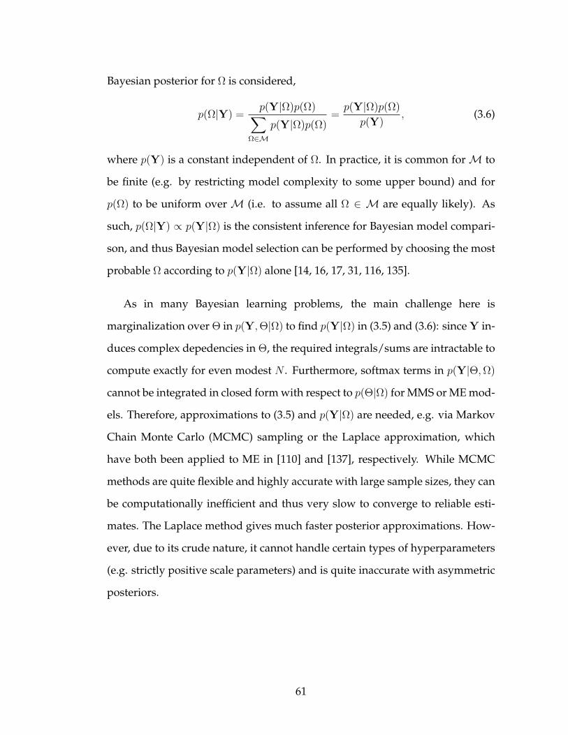
Bayesian posterior for ⌦ is considered,
p(⌦|Y) =
p(Y|⌦)p(⌦)X
⌦2M
p(Y|⌦)p(⌦)=
p(Y|⌦)p(⌦)p(Y)
, (3.6)
where p(Y) is a constant independent of ⌦. In practice, it is common for M to
be finite (e.g. by restricting model complexity to some upper bound) and for
p(⌦) to be uniform over M (i.e. to assume all ⌦ 2 M are equally likely). As
such, p(⌦|Y) / p(Y|⌦) is the consistent inference for Bayesian model compari-
son, and thus Bayesian model selection can be performed by choosing the most
probable ⌦ according to p(Y|⌦) alone [14, 16, 17, 31, 116, 135].
As in many Bayesian learning problems, the main challenge here is
marginalization over⇥ in p(Y,⇥|⌦) to find p(Y|⌦) in (3.5) and (3.6): since Y in-
duces complex depedencies in ⇥, the required integrals/sums are intractable to
compute exactly for even modest N . Furthermore, softmax terms in p(Y|⇥,⌦)cannot be integrated in closed form with respect to p(⇥|⌦) for MMS or ME mod-
els. Therefore, approximations to (3.5) and p(Y|⌦) are needed, e.g. via Markov
Chain Monte Carlo (MCMC) sampling or the Laplace approximation, which
have both been applied to ME in [110] and [137], respectively. While MCMC
methods are quite flexible and highly accurate with large sample sizes, they can
be computationally inefficient and thus very slow to converge to reliable esti-
mates. The Laplace method gives much faster posterior approximations. How-
ever, due to its crude nature, it cannot handle certain types of hyperparameters
(e.g. strictly positive scale parameters) and is quite inaccurate with asymmetric
posteriors.
61

3.2.4 Variational Bayes Approximations
Alternatively, variational Bayes (VB) approximations can be used. In the present
context, VB seeks to minimize the Kullback-Leibler divergence (KLD) functional
KL(q||p) = �Z
q(⇥|Y,⌦) log
⇢
p(⇥|Y,⌦)
q(⇥|Y,⌦)
�
d⇥ (3.7)
between an integrable and closed-form variational posterior parameter distri-
bution q(⇥|Y,⌦) and the true posterior parameter distribution p(⇥|Y,⌦), for
⌦ 2 M. Since (4.54) can be viewed as a ‘distance measure’ between two dis-
tributions, VB seeks a principled probabilistic approximation q to the true in-
tractable posterior p, where the conditional independence properties of q are
chosen a priori to ensure tractability. Eq. (4.54) is minimized in practice by max-
imizing a lower bound L to log p(Y|⌦), where it can be shown via Jensen’s in-
equality that [16]
log p(Y|⌦) = L+ KL(q||p), (3.8)
where L =
Z
q(⇥|Y,⌦) log
⇢
p(⇥,Y|⌦)q(⇥|Y,⌦)
�
d⇥ (3.9)
The property L log p(Y|⌦) follows from the fact that KL(q||p) � 0 for any
q and p. The VB posterior approximation q can be determined iteratively with
monotonically increasing L, such that q is guaranteed to converge on a local
minimizer of KL(q||p) [16]. Furthermore, since the maximizer of p(Y|⌦) also
maximizes log p(Y|⌦) and neither term is available in practice, L can be used to
approximate log p(Y|⌦) and thus serve as the metric to maximize for Bayesian
model selection [14, 16, 31, 57, 116]. Note that p can be multimodal due to com-
plex probabilistic dependencies between variables or non-identifiability issues,
so that q (which is often unimodal) can converge towards any one of p’s true
modes to (locally) minimize the KLD. Therefore, a common strategy to find-
62

ing the best KLD minimizer (also used in this work) is to apply multiple initial
guesses for q, e.g. using ML/MAP solutions.
Refs. [135] and [17] proposed VB approximations for ME regression models
(i.e. with continuous expert outputs in (3.4) instead of discrete ones), although
their methods have important drawbacks that severely limit their applicabil-
ity to ME and MMS discriminative models. In particular, the method of [135]:
(1) cannot use the softmax model, (2) cannot estimate expert model parameters
from data, and (3) requires density estimation of the joint input-output distri-
bution p(X,D), which is generally challenging and computationally expensive.
The method of [17] overcomes only the last two drawbacks, since it can only
be applied to ME models specified via trees of binary logistic gating and expert
functions. This requires M to contain all possible binary trees for fixed G, which
raises the overall cost of learning (especially if K > 2, since each expert must
also be expressed as a ‘one-vs-all’ binary classification tree). The limitations of
both these VB methods stem directly from analytical difficulties in handling the
softmax function. As such, they are ill-suited for learning general models with
latent softmax terms and are particularly unusable for learning MMS, which is
intrinsically defined by the softmax model.
To overcome these limitations, new VB approximations are proposed here
to handle softmax functions analytically using a bound proved in [20]. These
approximations place no restrictions on learning with latent softmax variables,
and are therefore easier to use and more broadly applicable than either of
the aforementioned VB methods for restricted ME models. In particular, it is
straightforward to extend the proposed VB approximations to hierarchical mix-
ture of expert discriminative and regression models, although the exact formu-
63

Z n
X n
D n
w i i
a 0
n = 1 :N
b 0i = 1 :S
Z n
X n
D n
w i i
a 0
n = 1 :N
b 0i = 1 :S
a 0
E n
X n
D n
u e e
n = 1 :N
b 0
e = 1 :G
w ec ecc0
d 0c = 1 :K
a 0
E n
X n
D n
u e e
n = 1 :N
b 0
e = 1 :G
w ec ecc0
d 0c = 1 :K
(a) (b)
Figure 3.2: Graphical plate models for Bayesian learning: (a) MMS, (b) ME.
las for these extensions are not given here due to limited space.
3.3 Variational Bayes Learning for MMS Models
The graphical model for Bayesian MMS learning is shown in Figure 3.2 (a),
for fixed ⌦ = [s1, ..., sK ] with labeled observations Y = {y1, ..., yN} =
{(x1, d1), ..., (xN
, dN
)} and hidden variables ⇥ = {Z1:N , w1:S,↵1:S} = {Z,w,↵}.
Defining D = {d1, ..., dN} and X = {x1, ..., xN
}, it follows from Figure 3.2 (a)
that
p(w,↵,Z,D|X) = p(↵)p(w|↵)
N
Y
n=1
p(Zn
|Xn
,w)p(Dn
|Zn
) (3.10)
For i 2 {1, ..., S}, n 2 {1, ..., N}, and dn
2 {1, ..., K}, the conditional distribu-
tions are assumed to be
p(↵i
; a0, b0) = G↵i(a0, b0), (3.11)
p(wi
|↵i
) = Nwi(0,↵
�1i
· I), (3.12)
p(Dn
= dn
|Zn
= i) = Tin
, (3.13)
p(Zn
= i|Xn
= xn
,w) = f(i; x,w), (3.14)
64

where G is the Gamma distribution with fixed shape and scale parameters a0
and b0. Note that each subclass weight wi
has a spherical zero-mean Gaussian
prior with a Gamma-distributed precision hyperparameter ↵i
; these conjugate
priors effectively enable regularization with an unknown penalty parameter
and are commonly used in Bayesian learning (e.g. see [16, 17, 116, 135]). Also
note that ↵i
need not be identical for all wi
, although this is assumed here for
simplicity.
From (3.5), the posterior over ⇥ is (dropping ⌦ for simplicity)
p(⇥|D,X) =
p(⇥,D|X)
p(D|X)
=
p(Z,w,↵,D|X)
P
z1:N
R R
p(Z,w,↵,D|X)dwd↵. (3.15)
Upon substitution of (3.10) - (3.14) into (3.15), it is clear that (3.15) is intractable
since p(D|X) requires an exponentially large sum over integrals that have no
closed form. To obtain a tractable approximate posterior q(⇥|Y,⌦) ⌘ q(⇥) =
q(Z,w,↵) using VB, q is first specified via an assumed conditional indepen-
dence factorization. The typical ‘mean-field’ approximation (e.g. [14, 17, 31,
116]) is used here, where
q(⇥) =N
Y
n=1
q(Zn
)
S
Y
i=1
q(wi
)q(↵i
) =
N+2SY
k=1
q(✓k
). (3.16)
This factorization is convenient since it can be shown through a standard proof
(e.g. Chapter 10 of [16]) that subsequent minimization of (4.54) leads to the
following canonical ‘free-form’ inference formula for each posterior factor ✓k
2⇥,
ln q(✓k
) = E [ln p(⇥,D|X)]
q(⇥\✓k) + const. (3.17)
The expectations here are taken on the log of (3.10) with respect to the varia-
tional posterior factors q(✓k
) of all hidden variables ✓k
in ⇥ except the ✓k
of in-
terest on the left hand side. Since the resulting formulas correspond to solving
65

simultaneous nonlinear equations, they are iteratively re-solved in cyclic fash-
ion until convergence. A single pass through (3.17) for each ✓k
is defined as one
VB cycle.
Now, the updates in (3.17) must be modified to handle the non-integrable
softmax terms from (3.14). These softmax terms are replaced by the local vari-
ational softmax lower-bound p(Zn
= i|Xn
= xn
,w) p(Zn
= i|Xn
= xn
,w)
proved in [20], where
p(Zn
= i|Xn
= xn
,w) = exp(wT
i
xn
� �n
), (3.18)
�
n
=�n
+
S
X
i=1
wT
i
xn
� �n
� ⇠in
2
+ �(⇠in
)[(wT
i
xn
� �n
)
2 � ⇠2in
] + log(1 + e⇠in), (3.19)
�(⇠in
) =
1
2⇠in
1
1 + e�⇠in� 1
2
�
. (3.20)
This lower bound replaces the non-integrable denominator of the softmax func-
tion in (3.14) with a product of unnormalized Gaussians, whose log is given
by (3.19). The scalars ⇠in
and �n
are local variational parameters that control the
shapes and locations of the bounding Gaussians across each training datum and
across each discrete label of the softmax distribution (the subclass labels, in the
MMS case). ⇠in
and �n
must be re-optimized within each VB cycle to tighten the
expected lower-bounds to the true softmax terms being approximated; fortu-
nately, this is done easily in closed-form with fairly tight bounds, as described
in [20]. It is easy to see that these local softmax lower bounds still ensure a lower
bound ˜L L to p(Y|⌦), where
˜L =
Z
q(⇥|Y,⌦) log
⇢
p(⇥,Y|⌦)q(⇥|Y,⌦)
�
d⇥,
p(⇥,Y|⌦) = p(↵)p(w|↵)
N
Y
n=1
p(Zn
|Xn
,w)p(Dn
|Zn
). (3.21)
66

Substituting (3.21) and (3.11)-(3.13) into (3.17) for (3.10) and computing the
required expectations leads to the following closed-form variational posterior
factors,
q(wi
) = Nwi(µi
,⌃i
), (3.22)
q(↵i
) = G↵i(ai, bi), (3.23)
q(Zn
= i) = g(i; xn
, {hw1i , ..., hwS
i}), (3.24)
where h·i is the expected value with respect to q(⇥), and
⌃
�1i
= h↵i
i · I + 2
N
X
n=1
�(⇠in
)xn
xT
n
, (3.25)
⌃
�1i
µi
=
N
X
n=1
htin
i � 1
2
+ 2�n
�(⇠in
)
�
xn
, (3.26)
ai
= a0 +M + 1
2
, bi
= b0 +1
2
⌦
wT
i
wi
↵
, (3.27)
htin
i = q(Zn
= i), h↵i
i = ai
/ bi
(3.28)
hwi
i = µi
,⌦
wT
i
wi
↵
= tr (⌃i
) + µT
i
µi
. (3.29)
Here, htin
i = q(Zn
= i) is subclass i’s expected posterior responsibility for training
datum n, which is computed via (3.3) using the expected subclass weights. As
shown in [20], the parameters ⇠in
and �n
can be set to maximize the expectation
of (3.18) with respect to q(⇥), giving
⇠2in
= xT
n
⌃
i
xn
+ (µT
i
xn
)
2+ �2
n
� 2�n
µi
xn
, (3.30)
�n
=
12(
S+12 � 1) +
P
S
i=1 �(⇠in)wT
i
xn
P
S
j=1 �(⇠jn). (3.31)
The lower bound ˜L to p(Y|⌦) can be computed to gauge convergence of the
67

VB cycles, where it can be shown that (for Tin
as defined in (3.3))
˜L =
N
X
n=1
(
log
S
X
i=1
Tin
· exp(µT
i
xn
)
!
� h�n
i)
�(
S
X
i=1
KL[q(wi
)||p(wi
| h↵i
i)] + KL[q(↵i
)||p(↵i
)]
)
. (3.32)
˜L represents an expected data log-likelihood penalized by the non-negative and
closed-form KLDs between the priors and variational posteriors 2. Most of the
required terms for ˜L are already computed during the cyclic updates for q(⇥)
and ˜L is also guaranteed to monotonically increase over the VB cycles.
Table 1 summarizes the VB learning procedure for fixed ⌦. Note that an
additional convergence loop of nlc
iterations is required here for the local vari-
ational parameters ⇠in
and �n
, which are coupled in (3.30)-(3.31); nlc
= 15 was
sufficient for this paper’s implementation. Since q(⇥) converges to a local KLD
minimizer, the VB algorithm should be run with multiple intializations to en-
sure ˜L is maximized for fixed ⌦ (this is the typical approach for avoiding poor
local solutions in VB learning, e.g. see [14, 17, 31, 116, 135]). In this paper’s im-
plementation, ⇠in
and �n
were initialized via (3.30) and (3.31) by replacing each
µi
with maximum likelihood weight estimates and ⌃i
with various spherical
covariances.
3.3.1 Bayesian MMS Model Selection
For each ⌦ = [s1, ..., sK ] in a set of candidate models M, the VB approximation
can be applied to find log p(Y|⌦) ⇡ ˜L⇤, where ˜L⇤=
˜L � ln(
Q
S
i=1 sd!) is the pe-2see Appendix B of [116] for the necessary Gaussian-Gaussian and Gamma-Gamma KLDs in
each prior/posterior pairing
68

Table 3.1: VB MMS Learning Algorithm for Fixed Subclass Configuration
0. Given: X, D, initial ⇠in
, �n
,
fixed subclass configuration with S total subclasses
1. for ⇠in
and �n
fixed for i 2 {1, ..., S}, n 2 {1, ..., N}
for i = 1 : S
compute q(wi
) using (3.22)
compute q(↵i
) using (3.23)
end
for n = 1 : N
compute q(Zn
) using (3.24)
end
2. for fixed q(⇥|X),
for i = 1 : nlc
(a) compute all ⇠in
for fixed �n
using (3.30)
(b) compute all �n
for all fixed ⇠in
using (3.31)
end
3. Compute ˜L using (3.32). Stop if ˜L converged; else, Repeat 1-2.
nalized lower bound obtained at convergence 3. M could be defined by placing
an upper bound r on sd
for each class d. However, this leads to rK possible
MMS models, which can be impractical to assess. Hence, heuristics are gener-3The penalty is needed since parameters are not identifiable if any s
d
> 1; the approximatemodel likelihood probability must be divided among all possible label permutations to correctlypenalize model complexity [34].
69

ally needed within the Bayesian model selection scheme (or any other model
selection strategy) to define M within practical limits for MMS.
A simple but principled ‘compressive search’ (CS) heuristic is proposed here
to define M iteratively via the posterior responsibilities htin
i from the VB ap-
proximation. This uses the idea that subclasses whose existence is not well-
supported by data are likely irrelevant and can probably be discarded. First,
the VB approximation is applied to the first r uniform subclass MMS models,
which have sd
= c 8d 2 {1, ..., K} and c 2 {1, ..., r}. Posterior subclass probabilities
(PSPs) are then estimated within each model for each original class label d and
relevant subclass i 2 �(d) by computing
p(i) =1
Nd
N
X
n=1
htin
i, (3.33)
which is the expected number of times i appears for all observed labels dn
= d
divided by Nd
, the number of training data with dn
= d. Note that htin
i = 0 if i /2�(d
n
), soP
i2�(dn) htini = 1 andP
i2�(d)P
N
n=1 htini =P
i2�(d)P
{n|d=dn} htini = Nd
;
hence,P
i2�(d) p(i) = 1 for each d. Next, the PSPs are thresholded against a user-
defined probability ✏ 2 [0, 1] to determine the number of ‘relevant’ subclasses
per class in each model. This results in an additional subclass configuration that
can be learned by VB on the next search iteration. The CS procedure stops when
either no new subclass models are formed or gmax
iterations are reached. The CS
method thus avoids brute force searches over rK MMS models by looking for
‘persistently useful’ subclasses over a smaller uniform block of models. Note
that the PSPs (3.33) resemble expected component responsibilities for Gaussian
mixtures [16], which is not surprising given the resemblences between MMS
and Gaussian mixture classifiers [3].
Table 3.2 summarizes the CS method, where r can be initialized to a modest
70

Table 3.2: Compressive Search for MMS Model Selection
0. Given: sd
upper bound r, max number of iterations gmax
� 1,
PSP threshold probability ✏, number of iterations g = 0
1. Set M to all uniform subclass configurations between 1 and r;
2. Define Mu
to be the set of models not yet learned in M;
3. Set g = g + 1 and for each configuration in Mu
:
perform VB learning using Table 1;
compute ˜L⇤=
˜L� ln(
Q
S
i=1 sd!);
compute p(i) for all subclasses using (3.33);
threshold p(i) against ✏ (subclass is relevant if p(i)� ✏);
count number of relevant subclasses sreld
per class label d;
set spawned configuration to [srel1 , ..., srelK
] and add to set Sg
4. If g < gmax
and Sg
[M 6= M, let M M [ Sg
and repeat 2-3;
Otherwise, stop;
5. Select ⌦ 2M with largest ˜L⇤.
value (e.g. 4 or 5) and then increased to scan more models, if required. Setting ✏
too large leads to overly conservative softmax models, while too small an ✏ can
spawn no models. Hence, ✏ should be in the range between which these two
extremes start occuring (which can be quickly estimated via bisection searches),
although this will be problem dependent and sensitive to small Nd
. In the exper-
iments here, ✏ 2 [0.01, 0.1] produced consistent results, though this range may
not be suitable in special cases (e.g. highly imbalanced data sets, which may re-
quire a separate ✏ for each class). The CS procedure forms at most r new models
71

per iteration g, so M has at most rgmax
models, which is linear in r and inde-
pendent of K. As the CS method is essentially top-down, the highest learning
cost is incurred by the r uniform subclass model, which can be used as a basis
for setting gmax
. In practice, CS should be run with multiple ✏ values in Step 3
to scan as many ‘interesting’ models as possible.
3.4 Variational Bayes Learning for ME Models
The graphical model for Bayesian mixture of experts (ME) learning is shown in
Figure 3.2 (b) for fixed ⌦ = G with labeled observations Y and hidden vari-
ables ⇥ = {E1:N , u1:G, w11:GK
,↵1:G, �11:GK
} = {E,u,w,↵,�}. There are two key
changes to the multimodal softmax VB approximation for ME learning: (1) the
softmax lower bound is applied G + 1 times: once for each of the G softmax
expert models and once for the softmax gating function, (2) separate priors, hy-
perparameters and hyperpriors are specified for the gating weights and the G
sets of expert weights.
The joint pdf for the ME model Figure 3.2 (b) given X is
p(E,D,u,w,↵, �1:G|X) = p(↵)p(�)p(u|�)p(w|↵)
⇥N
Y
n=1
G
Y
g=1
"
p(En
= g|Xn
,u)K
Y
d=1
[p(Dn
= d|Xn
, En
,w)]
sdn
#
tgn
(3.34)
where sdn
and tgn
are binary indicator variables denoting membership of da-
tum n to the states Dn
= d and En
= g, respectively (sdn
is observed in the
training data through D; tgn
is hidden since En
is hidden). For g 2 {1, ..., G},
c 2 {1, ..., K}, and n 2 {1, ..., N}, the distributions are
p(↵g
) = G↵g(a0, b0), (3.35)
p(�gc
) = G�gc(c0, d0), (3.36)
72

p(ug
|↵g
) = Nug(0,↵
�1g
· I), (3.37)
p(wgc
|�gc
) = Nwgc(0, �
�1gc
· I), (3.38)
p(En
= g|Xn
= x,u) = f(g; x,u), (3.39)
p(Dn
= d|Xn
= x,En
= g,w) = f(d; x, wg1:gK). (3.40)
From (3.5), the posterior over the hidden variables⇥ = {E,u,w,↵,�} takes ex-
actly the same form as (3.15), where the denominator is now given by marginal-
ization of (3.34) over the ⇥ variables. Once again, substitution of (3.35)-(3.40)
into (3.15) leads to an intractable posterior, as in the MMS case. The VB ap-
proximation thus proceeds as before, although now the following factorized
approximate posterior is assumed,
q(⇥) =G
Y
g=1
"
q(↵g
)q(ug
)
K
Y
c=1
q(�gc
)q(wgc
)
#
N
Y
n=1
q(En
)q(Dn
)
=
2N+2G(K+1)Y
k=1
q(✓k
), (3.41)
which again leads to the variational posterior factor update formulas from
(3.17), where the joint pdf is now given by (3.34). However, to obtain closed-
form expectations, the softmax lower bound (3.18) is now applied G+1 separate
times to replace the (3.39) and (3.40) terms in (3.34). To this end, let the lower
bounding softmax replacements be denoted by
p(En
= g|x,u) = exp(uT
g
x� �0n
(�0n
, ⇠1:Gn
)), (3.42)
p(Dn
= d|x, g,w) = exp(wT
gd
x� �g
n
(�g
n
, ⇠g1:gKn
)) (3.43)
where the relations from (3.19)-(3.20) still apply for g 2 {1, ..., G}, d 2 {1, ..., K},
and where�
�0n
, ⇠1:Gn
and�
�g
n
, ⇠g1:gKn
are the corresponding sets of variational
parameters for the gating lower bound and the gth expert’s lower bound, re-
spectively (note that there are now a total of 2N + NG(K + 1) local variational
parameters).
73

Substituting (3.42), (3.43), and (3.35)-(3.38) into (3.34) and computing the re-
quired expectations in (3.17) via (3.41) leads to the following closed-form varia-
tional posterior factors,
q(ug
) = Nug(µg
,⌃g
), (3.44)
q(↵g
) = G↵g(ag, bg), (3.45)
q(wgc
) = Nwgc(µgc
,⌃gc
), (3.46)
q(�wg
) = G�gc(cgx, dgc), (3.47)
q(En
= g) = f(g; [xn
, 1]T {vn1, ..., vnG}), (3.48)
where
⌃
g
= h↵g
i · I + 2
N
X
n=1
�(⇠gn
)xn
xT
n
(3.49)
⌃
�1g
µg
=
N
X
n=1
htgn
i � 1
2
+ 2�0n
�(⇠ggn
)
�
xn
(3.50)
⌃
gc
= h�gc
i · I + 2
N
X
n=1
htgn
i�(⇠gcn
)xn
xT
n
(3.51)
⌃
�1gc
µgc
=
N
X
n=1
htgn
i
sdn
� 1
2
+ 2�g
n
�(⇠gcn
)
�
xn
(3.52)
vng
= [µg
+ µgh
, �h�g
n
i]T , where h = dn
(3.53)
ag
= a0 +M/2, bg
= b0 +1
2
⌦
uT
g
ug
↵
(3.54)
cgc
= c0 +M/2, dgc
= d0 +1
2
⌦
wT
gc
wgc
↵
(3.55)
htgn
i = q(En
= g), h↵g
i = ag
/bg
, h�gc
i = cgc
/dgc
(3.56)⌦
uT
g
ug
↵
= tr (⌃g
) + µT
g
µg
,⌦
wT
gc
wgc
↵
= tr (⌃gc
) + µT
gc
µgc
(3.57)
The updates for the local gating and expert variational parameters are the same
as in (3.30) and (3.31) with µi
and ⌃i
replaced: the updates for ⇠gn
and �0n
use µg
and ⌃g
, while the updates for ⇠gnn
and �g
n
use µgc
and ⌃gc
. To assess convergence
74

of VB iterations, ˜L can be computed as
˜L =
N
X
n=1
G
X
g=1
"
htgn
iµT
g
xn
+
K
X
c=1
htgn
i sdn
µT
gn
xn
#
+H[q(E)]�
N
X
n=1
"
⌦
�
0n
↵
+
G
X
g=1
htdn
i h�g
n
i#!
� KL[q(↵)||p(↵)]� KL[q(�)||p(�)]
� KL[q(u)||p(u| h↵i)]� KL[q(w)||p(w| h�i)], (3.58)
where H[q(E)] is the Shannon entropy of q(E) =
Q
N
n=1 q(En
) (note that each
q(En
) is a discrete distribution and the KLDs are again closed-form, as per foot-
note 2). Table 3 summarizes the VB learning procedure for ME, which should
be run with different initializations to avoid poor local solutions. As with MMS
learning, maximum likelihood ME weight estimates are used here to intialize
the local variational parameters for (3.42) and (3.43) for multiple runs. As be-
fore, nlc
= 15 was sufficient for the experiments here.
3.4.1 Bayesian ME Model Selection
Compared with the MMS model, the ME model space is much simpler to con-
sider; a natural choice for M is the set of ME models with ⌦ = G between
1 and some upper bound. The VB approximation of Table 3 can be applied
to each ⌦ 2 M to obtain the penalized VB model log-likelihood lower bound
˜L⇤=
˜L � lnG! (which accounts for hidden expert label permutations). The ⌦
with the largest ˜L⇤ can then be selected as the best fit.
75

3.5 Experimental Results
This section presents VB learning results for MMS and ME on four benchmark
data sets from classification literature and two data sets from an experimental
application. Ten randomized training sets were created in each case to simulate
multiple learning instances with the ‘raw’ X space, using no feature process-
ing other than simple normalization. In all cases, the shape and scale prior
hyperparameters for VB learning were set to a0 = b0 = c0 = d0 = 1
4, and
the convergence tolerance on ˜L was set to 1 ⇥ 10
�3 over 600 maximum update
cycles. Maximum likelihood estimates were used to initialize all VB learning
algorithms (as described in Secs. 3.3 and 3.4) except for the second phase of
compressive searches (CS) for MMS, in which relevant parent subclass weights
were used instead. Models learned by VB were also compared to those obtained
by maximum likelihood (ML) and the Bayes Information Criterion (BIC) score,
BIC(⌦) = log(L⌦)� 1
2
k⌦ log(N)� 1
2
C(⌦), (3.59)
where L⌦ is the maximized likelihood for model ⌦, k⌦ is the free parame-
ter count and C⌦ is the model permutation penalty. BIC is a popular metric
for probabilistic model selection with hidden variables [14, 29, 34, 116]; as [14]
notes, (3.59) asymptotically approximates log p(Y|⌦) and can be seen as a lim-
iting case of the VB lower bound for N ! 1. Thus, (3.59) is a suitable fitness
metric to compare against the VB lower bound ˜L⇤. All experiments were run in
MATLAB (2.41 GHz AMD Athlon processor, Windows XP, 1.96 GB of RAM).
Since the generating models for the data are unknown, more sophisticated
nonlinear kernel classifier models were used as ‘high baselines’ to assess the
quality of the learned MMS and ME models by comparing holdout classification4the results were insensitive to these values, i.e. similar learning results were obtained with
much broader gamma hyperpriors.
76

1 2 3 4 5!600
!550
!500
!450
!400
!350
!300
!250
!200
!150
!100BANANA Approx. Model Log!likelihoods
Number of Uniform Subclasses (MMS) or Number of Experts (ME)
App
roxi
mat
e M
odel
Log
!lik
elih
ood
ME VBMMS VBME BICMMS BIC
1 2 3 4!180
!160
!140
!120
!100
!80
!60
!40THYROID Approx. Model Log!likelihoods
Number of Uniform Subclasses (MMS) or Number of Experts (ME)
App
roxi
mat
e M
odel
Log
!lik
elih
ood
ME VBMMS VBME BICMMS BIC
1 2 3 4!1200
!1100
!1000
!900
!800
!700
!600
!500
!400
!300
!200IMAGE Approx. Model Log!likelihoods
Number of Uniform Subclasses (MMS) or Number of Experts (ME)
App
roxi
mat
e M
odel
Log
!lik
elih
ood
ME VBMMS VBME BICMMS BIC
(a) Banana (b) Thyroid (c) Image
Figure 3.3: Selected MMS and ME learning results on benchmark data (uniformMMS configurations shown only).
error rates. It is emphasized here that model selection is the focus of this study
and these error rates are included only for completeness.
3.5.1 Benchmark Data
Four binary class data sets were taken from the Ratsch benchmark set [113],
which is often used to compare sparse nonlinear kernel classifiers (e.g. [132, 68]).
Hence, these data offer a good challenge for Bayesian learning of ‘standard’
MMS and ME models that can only construct piecewise linear log-odds bound-
aries (cf. Section 2). The benchmarks used here are5: Banana (2 dimensions,
5400 total data points, 400 training points), Thyroid (5 dimensions, 215 total, 140
training), Image (20 dimensions, 2310 total, 1300 training), and Twonorm (20 di-
mensions, 7000 total, 400 training). In all cases, ME models were learned for all
G 2 [1, 5] and MMS models were learned for all sd
5. The compressive search
(CS) in Table 3.2 was also used separately with r = 5 and gmax
= 2 (so that at
most 10 models could be assessed in each case). All sets used ✏ = 0.05 except
Thyroid, where ✏ = 0.10 to due to less available data. Table 3.4 summarizes the5the training/validation splits were tabulated previously in a standard catalog.
77

benchmark learning results, where classification error rates for the VB-learned
models with the highest average ˜L⇤ are computed with MAP parameters (errors
via eq. (3.1) with ML weights are also shown for a ‘low-baseline’ comparison).
Also shown for the CS results are: the number of times non-uniform VB-selected
MMS models are scanned over all instances (#sc.); the average number of par-
ents for the best-fit VB model (pa); and the maximum number of models as-
sessed by CS across all instances (|M|max). Figure 3.3 plots some of the average
˜L⇤ and BIC model scores for ME and MMS.
Figure 3.3 shows that both scores generally behave similarly for MMS and
ME as a function of complexity, as expected from theory. Interestingly, BIC is
more conservative for the ME Twonorm case and less conservative for the MMS
Thyroid case. In the former case, the complexity of the ME model dominates the
BIC score, leading to a very stiff penalty. In the latter case, complex MMS mod-
els are often able to overfit with large enough L⌦ in (3.59) to counteract small
fixed k⌦ and C⌦ penalties. VB avoids these issues and behaves more consis-
tently in all cases due to ˜L⇤ ’s adaptive penalty structure, which also accounts
for estimated parameter magnitude. The MMS and ME models selected by VB in
Table 3.4 also show better agreement with each other, as the maximum sd
closely
matches G in each case. This is reassuring, given the similarities between MMS
and ME [3].
The error rates can be compared to the following literature results for non-
linear kernel classifiers: Banana: 10.8% and Image: 3.9% (both RVMs) [132] ;
Thyroid: 4.3% and Twonorm: 2.6% (both Laplacian classifiers) [68]. From these
baselines, it is easy to see that the models learned by VB are reasonable and
accurate. Since MMS and ME only use piecewise-linear class boundaries here,
78

the errors in Table 3.4 are expected to be somewhat higher than these baselines
(which used much more highly optimized complex class boundaries), although
they are still fairly close for these data. The models learned by VB and ML/BIC
generally performed similarly (i.e. < 1% error difference), with some excep-
tions. The [1,2] MMS model ‘selected’ by ML/BIC for Twonorm leads to 12.27%
error, while the ML/BIC-selected G = 2 ME models for Image and Thyroid give
errors of 7.33% and 13.37%, respectively. The former result stems from poor BIC
penalization. The latter results are due to ML overfitting, as evidenced by the
fact that VB selects G = 2 in both sets while achieving smaller errors (the ML
weights are two orders of magnitude larger).
Table 4 also shows that CS searches over no more than 6 models to con-
sistently find MMS models that are the same as/very close to the best mod-
els obtained by VB with a more expensive brute force search. The results for
pa also show that complex higher order models are frequently compressed to
lower orders (e.g. for Banana, pa = 1.8 is reasonable for [3,3] since it can only be
spawned by two models: [4,4] and [5,5]). Varying ✏ between [0.01, 0.1] and/or
setting gmax
= 3 did not change the set of scanned models significantly (Thyroid
was similarly insensitive for ✏ 2 [0.01, 0.36]). The slight disagreement between
brute force and CS for Image gives a small 0.12% difference in classification error,
though it is worth noting that CS never spawns the [3,1] model (altering ✏ or g
did not change this).
3.5.2 RoboFlag Data
The application data come from an experimental human-robotic interaction
study, in which 16 human operators were trained to play 20 games of ‘capture
79

the flag’ with robots in the RoboFlag simulator program [27]. In each game, a
single player assigned waypoint locations for three robots over a search field
in order to locate/identify two enemy targets, while avoiding collisions and a
mobile enemy chaser. All telemetry and waypoint data from each game was
recorded. These were post-processed by hand-labeling each assigned waypoint
as one of several discrete high-level operator strategies that were commonly ob-
served during the game. The ones considered here are (with number of total
instances):
• Strat: move robot to strategic place for later use (1277)
• Dcy: use robot to decoy chaser (1156)
• Srch: use robot to search for targets (1034)
• ID/Loc: use robot to identify/localize targets (1674)
• Evas: avoid collision between robot and enemy (736).
These data are used to learn P (D|X) via latent softmax variables, where
X is a 10-dimensional vector of continuous telemetry data (relative posi-
tions/orientations of all vehicles) and D is a discrete strategy given X . Ten
training instances of two different decision data subsets were used with 300
training data points per class: Case 1 with classes [Dcy, Srch, ID/Loc], and Case
2 with classes [Evas, Strat, Srch]. Further details on the experimental data and
the motivation for learning P (D|X) in the context of hybrid Bayesian network
modeling can be found in [22] and [27]. ME models were learned for all G be-
tween 1 and 6. CS was applied to each case with r = 6, ✏ = 0.05 and gmax
= 2 to
generate M for MMS.
80

1 2 3 4 5 6
!1150
!1100
!1050
!1000
!950
!900
!850
!800
!750
!700
!650
RF1SET1 and RF1SET2 Approx. Model Log-likelihoods
Number of Experts (ME) or Number of Uniform Subclasses (MMS)
Appr
oxim
ate
Mod
el L
og!l
ikel
ihoo
d
Case 1 ME VBCase 1 MMS VBCase 2 ME VBCase 2 MMS VB
Figure 3.4: VB model log-likelihoods for RoboFlag cases 1 and 2 (uniform MMSconfigurations shown only).
Table 3.5 summarizes the learning results, with classification error rates for
high-baseline nonlinear kernel SVM classifiers (N-SVM, with Gaussian kernels
whose bandwidths were set via cross-validation) and low-baseline basic soft-
max models (trained via ML). Figure 3.4 plots some ˜L⇤ values from MMS and
ME learning. The VB-learned MMS and ME models are comparably accurate
to each other and the N-SVM classifiers (the modest error rates for the N-SVMs
reflect the inherent difficulty of separating the decision classes using teleme-
try data alone). Thus, the VB models are indeed reasonable and unlikely to be
overfit. The models selected by ML/BIC show good agreement with ˜L⇤ in both
cases for the MMS model. This is not the case for the ME model: ML/BIC heav-
ily overpenalizes model complexity and always selects the basic softmax model
(G = 1), which is least accurate in both cases. Figure 3.4 shows that ˜L⇤ is gener-
ally higher for MMS than for ME. This is due to the dimension of X , which leads
to heavier penalties in (3.58). Table 3.5 also shows that CS searches over 10 or
fewer models in each case. While the [1,2,2] model is scanned in all instances by
CS for both Case 1 and 2, the [1,3,2] model in Case 2 (which has slightly lower
classification error and slightly higher ˜L⇤ ) is scanned in only half the instances
81

(altering ✏ and gmax
did not force [1,3,2] to appear in the other half or change
pa). The CS results for Cases 1 and 2 were consistent for ✏ 2 [0.015, 0.11] and
✏ 2 [0.02, 0.08], respectively.
3.5.3 Performance Times
Table 3.6 shows average computation times for VB and ML/BIC learning for
the ‘non-basic’ models selected via ˜L⇤ in Tables 3.4 and 3.5 6. The ML results
used direct nonlinear optimization via Matlab’s quasi-Newton fminunc rou-
tine (the Hessian was computed explicitly for MMS and automatically approx-
imated for ME). It is clear that direct ML is faster than VB on low-dimensional
problems such as Banana, although the times increase (mainly for ME) as the
problem dimensions increase 7. The times required for the VB approximations
are reasonable, especially for the higher dimensional problems (as the factor-
ized mean-field approximation advantageously decouples complex parametric
dependencies).6A comparison of the times for the baseline nonlinear kernel models is not feasible, as these
times are either not available in the literature or cannot be directly compared to m-code execu-tion times (e.g. the N-SVM used highly optimized compiled C code)
7turning off Hessian computations sped up ML greatly, although it converged to poor localmaxima much more frequently
82

3.6 Discussion
3.6.1 Performance Considerations
While a full analysis cannot be given here due to space limitations, some com-
ments are in order regarding sample size sensitivity for the proposed VB ap-
proximations. Further trials (not presented here) on the data of Sec. 4.5, on
synthetic truth data and on more complex/highly sparse benchmark data (e.g.
the Forensic Glass set [9]) suggest that the proposed mean field VB approxima-
tions can perform badly with very sparse data sets and are instead most reliable
for intermediate and large sample sizes (i.e. relative to the number of parame-
ters to be estimated). This agrees with the findings of previous empirical and
theoretical studies on the asymptotic properties of mean field VB approxima-
tions in other related models [35, 60, 136], which show that VB estimates are
generally biased with respect to the true posterior statistics (as an unavoidable
consequence of ‘deliberate model misspecification’ via the mean field assump-
tion). While such biases can be quite significant at small sample sizes, they
generally become much less significant as the proportion of observed to unob-
served variables in the training set increases (or equivalently, as the number of
training data increases when the number of hidden parameters can be fixed, as
in the models studied here). As noted in ref. [14], sparse data can cause signif-
icant difficulties even for state-of-the-art sampling algorithms, which typically
require more effort to tune and are more computationally expensive than VB for
fully Bayesian learning.
Since latent softmax models are useful for pure classification as well as gen-
eral hybrid probabilistic modeling (cf. Section 4.1), it should also be noted that
83

models selected to maximize the VB lower bound ˜L⇤ are not necessarily guar-
anteed to minimize classification error rate (as these metrics are not the same
[16]). For instance, it was found that the [4,3] model learned by VB had the
best overall MMS error rate for Banana (12%), despite having a slightly lower
˜L⇤ score than the [3,3] model. Thus, the proposed VB approximations should
be used appropriately. If the goal is to optimize classifier accuracy, then esti-
mated classification error should be used as the fitness metric, if possible [85].
While VB can always be used to approximate (3.5) for Bayesian classification,
˜L⇤ should only be used for classifier selection if reliable error rate estimates are
infeasible/expensive to obtain [17]. In contrast, ˜L⇤ should always be used in
general Bayesian network identification problems, since (approximate) model
log-likelihoods are of direct interest [14, 99].
Regarding MMS model selection, it should be emphasized that the proposed
compressive search (CS) is only a simple suboptimal heuristic for avoiding brute
force comparisons over an exponentially large model space. As such, it has
no formal guarantee of finding an MMS model to maximumize ˜L⇤ . Although
CS does well here overall at scanning suitable MMS models with limited data,
the results nevertheless point to some limitations. Firstly, as (3.33) suggests, CS
requires each class to have sufficient data for the estimates in (3.33) to be reliable.
Secondly, CS can get trapped with extra subclasses due to highly nonlinear class
boundaries in X (e.g. CS is unable to compress [3,2] to [3,1] in the Image results).
Therefore, while CS generally searches in the ‘best neighborhood’ of models
(given enough data), it may not fully explore this neighborhood. Running CS
with multiple ✏ values per class can sometimes remedy this, though post-hoc
analysis of scanned models often yields better insight for improving searches 8.8e.g. if s
d
= 1 is always spawned for certain classes, then a constrained brute force searchmay be feasible over other classes
84

Although beyond the scope of this paper, it is also possible to consider ˜L⇤ as a
score for other model search strategies (e.g. greedy searches [135]).
3.6.2 Extensions
The proposed VB approximations can be readily extended to hierarchical ME
models (cf. Section 2), where the local variational softmax bound can be applied
to every softmax gating/expert function in a mean-field approximation. The
proposed methods can also be extended to softmax-gated ME regression models
by replacing the softmax experts in (3.4) with linear-Gaussian output models
(e.g. see [17]). This replacement is particularly nice as it eliminates the local
softmax bound G times (it must only be applied for the gating function). The
proposed VB approximations can also be used if X is replaced by an arbitrary
nonlinear input map �(X) (e.g. from feature selection or basis changes). As
such, the lower bound ˜L⇤ can also be very useful for comparing models with
different �(X).
In light of these extensions, it is important to note that VB approximations
are always prone to poor local KLD minimizers. The implementations here
largely mitigated this via multiple initializations derived from maximum like-
lihood (ML) estimates (e.g. see [116]). Although ML is also prone to poor lo-
cal solutions, it can often be quickly re-run many times using direct optimiza-
tion methods to obtain a good set of a priori initial guesses for VB. However,
this strategy can be infeasible for problems involving very high-dimensional
parameter spaces and/or hierarchical models. While avoidance of poor local
solutions can never be fully guaranteed, it is straightforward to slightly modify
the general mean-field VB updates in (3.17) to accommodate the deterministic
85

annealing approach of [74], which can effectively mitigate VB’s sensitivity to
poor initializations (a similar method is also defined in [57] for VB learning).
3.7 Conclusions
This paper derived new variational Bayes (VB) learning approximations for two
latent softmax variable models: the multimodal softmax model and the mix-
ture of expert discriminative models. The proposed VB solutions overcome the
limitations of previous Bayesian methods for learning latent softmax variable
models, and are also readily extendable to hierarchical mixture of expert mod-
els for classification and nonlinear/non-Gaussian regression. Experiments with
benchmark and application data showed that the proposed VB approximations
are effective in practice. Comparisons to models learned via the Bayes Informa-
tion Criterion and to baseline nonlinear kernel classifiers confirmed the sound-
ness of the proposed VB approximations for Bayesian parameter estimation and
model selection.
86

Table 3.3: VB ME Learning Algorithm for Fixed G
0. Given: X, D, number of experts G, initial ⇠gn
, �0n
, ⇠gdn
, and �g
n
1. for ⇠gn
, ⇠gdn
, �0n
and �g
n
fixed for g 2 {1, ..., G}, d 2 {1, ..., K},
and n 2 {1, ..., N}
for g = 1 : G
compute q(ug
) using (3.44)
compute q(↵g
) using (3.45)
for d = 1 : K
compute q(wgd
) using (3.46)
compute q(�gd
) using (3.47)
end
end
for n = 1 : N
compute q(En
) using (3.48)
end
2. for fixed q(⇥|X),
for i = 1 : nlc
(a) update all ⇠gn
and ⇠gdn
for all fixed �0n
and �g
n
(b) update all �0n
and �g
n
for all fixed ⇠gn
and ⇠gdn
end
3. Compute ˜L using (3.58). Stop if ˜L converged; else, Repeat 1-2.
87

Table 3.4: Benchmark Learning Results (MMS: best [s1, ..., sK ] from brute force (BF) andcompressive search (CS) shown; ME: best G shown)
DataMMS ME Eq. (3.1)
BIC-BF VB-BF VB-CS (#sc., pa, |M|max) VB-CS % Error BIC VB VB %Error ML %Error
Banana [4,3] [3,3] [3,3] (-,1.5,6) 13.01±0.73 3 4/3 12.60±0.98 (G=4) 47.63 ± 4.17
Thyroid [2,1] [2,1] [2,1] (10,4,6) 5.60±2.65 1 2 5.20±3.17 12.53 ± 4.71
Image [3,1] [3,1] [3,2] (10,1.8,6) 3.40±0.57 2 3/2 3.69±0.88 (G=3) 48.81 ± 9.71
Twonorm [1,1]/[1,2]/[2,1] [1,1] [1,1] (-,4,5) 3.06±0.36 1 1 3.06±0.36 4.26 ± 0.68
Table 3.5: MMS/ME Learning Results for RoboFlag Data (MMS BIC/VB results for CS-generated models)
CaseMMS ME N-SVM Eq. (3.1)
BIC VB (#sc., pa, |M|max) VB %Error BIC VB VB %Error %Error ML %Error
1 [1,2,2] [1,2,2] (10, 3.6, 8) 16.33±0.34 1 2 16.02±0.35 15.71±0.48 19.09±0.63
2 [1,2,2] [1,2,2]/[1,3,2] (10/5,2.1/0.9,10) 18.44±0.45 / 17.92±1.05 1 3 18.10±1.03 18.53±0.83 23.23±0.68
Table 3.6: Mean learning times for models selected by VB (secs).
DataMMS (CS selection) ME
ML VB ML VB
Banana 0.25 5.91 0.84 4.83
Thyroid 0.20 1.49 2.92 1.64
Image 39.98 24.95 209.70 14.91
RF 1 1.79 12.92 32.24 10.83
RF 2 1.16 16.30 27.59 10.84
88

CHAPTER 4
HYBRID BAYESIAN INFERENCE FOR SOFT INFORMATION FUSION IN
HUMAN-ROBOT COLLABORATION
4.1 Introduction
In order to behave intelligently in complex environments, autonomous robots
must continuously update their understanding of the world by combining new
pieces of information from various sources. Despite considerable advances in
autonomous robot control and sensing in the last decade, human inputs are
still required in most practical settings to overcome various perceptual limita-
tions and ensure robustness in the presence of uncertainties. As such, data fusion
plays an important role in the application of collaborative human-robot teams
to diverse areas such as defense and security [18], search and rescue [21], space
exploration [54], and social robotics [12]. In the information-sharing context, hu-
mans are typically treated as sensors that describe high-level phenomena only.
That is, outside of commanding robots in control tasks such as low-level teleop-
eration or high-level planning, humans are only expected to provide crisp obser-
vations about discrete abstract world states, such as behavioral goals/intentions
or object/place classes [134]. In addition, low-level continuous world states are
expected only to be described by well-defined data obtained directly from robot
sensors. While this split high-level/low-level data fusion approach underscores
the primary strengths of human and robot perception, it also emphasizes the
consumption of concrete ‘hard’ information only. The fact that humans are rich
sources of potentially useful ‘soft’ information is thus frequently overlooked in
the data fusion problem.
89

Though less precise than conventional hard sensor data, soft low-level sen-
sor data in the form ‘negative measurements’ have already proved quite use-
ful for robotic mapping [131], localization [64], and object tracking [81, 118].
However, little work has been done on fusing soft low-level information from
humans with hard/soft data from robot sensors. As noted by Hall and Jordan
[59], a key issue that must be addressed in using ‘soft human sensors’ is that
of data characterization and representation; soft human information is highly
context-specific and is usually related through imprecise/‘fuzzy’ terminology,
as in the statements:
• ‘The car is moving quickly around the block; a bike is close behind it’
• ‘The truck is to the left of me’
• ‘Nothing is behind the building or on top of the roof’
• ‘The sidewalk is very steep; the nearby obstacle is much lighter than the
robot’.
Furthermore, although humans are subject to extrinsic uncertainties that also af-
fect conventional hard sensors (e.g. weather, observation conditions), humans
are subject to markedly different intrinsic biases and uncertainties via psycho-
logical/cognitive factors (e.g. expertise level; susceptibility to stress and fa-
tigue; memory and response capacities), and they are also not guaranteed to
provide information in a fully consistent or predictable manner. Despite these
challenges, soft human inputs have been successfully exploited for interactive
robot navigation and planning [12, 127, 84, 65]. These methods, however, treat
human inputs as sources of robot control commands/constraints only (e.g.‘go
around the table and between the chairs’) and therefore do not address the more
90

general problem of extracting and sharing low-level information derived from
purely observational statements about arbitrary world states (such as those
listed above). To this end, the robot’s underlying data fusion process must be
adapted to accomodate soft human information sources.
The problem considered here is the dynamic fusion of ambiguous human-
provided soft descriptions of continuous unknown world states (e.g. object lo-
cation, velocity and/or mass, as in the above examples) with conventional robot
sensor data. Depending on the application, the states of interest may not always
be observable through the robot’s sensors alone. For instance, as discussed in
[80], a robot equipped with a 2D horizontal scanning lidar can track the position
and velocity of moving people, but will not have direct access to height, weight
or goal location information that could be used to improve target motion mod-
els. Furthermore, all states become unobservable if targets are occluded or move
out of sensor range for a long time. By acting as an externally available soft sen-
sor in such cases, a helpful human agent can provide the robot with relevant
information that substantially reduces uncertainty or inconsistencies in target
state belief (e.g. due to poor/reduced observability or previous fusion of faulty
information).
The integration of human-robot information sources for cooperative percep-
tion and estimation has been previously considered in the context of applica-
tions such as navigation via social interaction [97], target tracking and surveil-
lance [75], and search-and-rescue [89]. Yet, few formal methods have been pro-
posed for fusing low-level human-robot data within the Bayesian framework,
which is popular for a wide range of autonomous estimation [131, 118, 24] and
human-robot interaction problems [79]. Refs. [78, 77] developed a Bayesian
91

method for fusing human-generated continuous range and bearing estimates
to tracked objects by modeling human sensors via linear-Gaussian regression
models, which were then incorporated into Kalman filters. Ref. [76] extended
this work to include probabilistic models of human visual sensing, which were
used to improve data association and object classification accuracy in joint
human-robot tracking tasks. Ref. [23] considered grid-based Bayesian fusion
of human target detection for a distributed 2D search problem, where human
field of view is modeled as a soft binary ‘detection/no detection’ sensor likeli-
hood model (akin to the UAV visual detection models of [21, 118]). While the
fusion methods developed in these previous works are formally Bayesian, they
are not general enough to efficiently handle soft low-level observations from a
human sensor. Indeed, despite the tendency of humans to softly categorize con-
tinuous data as a convenient means for sharing and processing complex infor-
mation (e.g. ‘near the landmark’ vs. ‘far from the landmark’), efficient Bayesian
fusion of such soft information is challenging from both a modeling and im-
plementation perspective. Although non-Bayesian fusion approaches based on
possibilistic fuzzy set theory could be used instead [126], it has been shown that
Bayesian methods are generally superior for dynamic data fusion [28]. Mixed
‘fuzzy-Bayesian’ approaches have also been considered; for instance, [93] pro-
poses random finite set-based ‘Kalman evidential filters’ for linear systems that
assign Gaussian fuzzy memberships to noiseless linear base measurements (this
method was also used in [80]). However, the measurement models assumed
by this approach require the identification of noiseless linear base measure-
ment functions and cannot describe highly ambiguous reports that induce non-
Gaussian state uncertainties or non-linear/non-convex state-to-data dependen-
cies (e.g. non-convex location rings from a range-only report such as ‘the car is
92

somewhat far from me’).
This paper proposes a new recursive hybrid Bayesian fusion framework for
efficiently combining conventional robot sensor data with human-generated
soft categorical information about continuous states. In contrast to previous
approaches, it is shown here that such human information can be modeled
via discrete random variables that are conditionally dependent on the continu-
ous states of interest through hybrid softmax likelihood functions (Section 4.2).
While these likelihoods allow for flexible and easily learnable representations of
soft human information, they also lead to analytically intractable Bayesian up-
dates for the continuous state. A new variational Bayesian importance sampling
(VBIS) algorithm is proposed here to approximate the true hybrid Bayesian pos-
terior as a Gaussian pdf in the baseline case of a basic softmax likelihood and
Gaussian state prior (Section 4.3). This baseline approximation is then extended
to produce Gaussian mixture posteriors for more general fusion scenarios in-
volving extended softmax likelihoods and Gaussian mixture priors, which can
compactly represent arbitrarily complex soft measurements and beliefs over
the states (Section 4.4). The utility and accuracy of the proposed methods are
demonstrated through online multi-target search experiments involving a coop-
erative human-robot team operating under various fusion conditions (Section
4.5). The experimental results are used to assess human-robot search perfor-
mance and the accuracy of the VBIS approximation across different types of
sensing modalities and prior information. Finally, Section 4.6 summarizes rele-
vant insights, extensions and conclusions for general human-robot information
fusion applications.
93

4.2 Preliminaries
4.2.1 General Problem Statement
The Bayesian data fusion approach proposed here equates soft descriptions of
continuous states with discrete random variables representing contextually dis-
tinct sets of state categorizations. These discrete random variable mappings can
be modeled directly via flexible ‘continuous-to-discrete’ hybrid likelihood func-
tions, thus enabling recursive Bayesian estimation of the unknown continuous
states.
For discrete time index k 2 Z0+, let Xk
2 Rn be the continuous random state
vector of interest with prior probability density function (pdf) p(X0) and transi-
tion pdf p(Xk
|Xk�1) arising from known stochastic dynamics. Furthermore, let
⇣k
2 Rnr,h⇥Znr,s be a mixed vector of nh,r
hard continuous robot sensor data (e.g.
lidar returns) and ns,r
discrete soft sensor data (e.g. ‘detection/no detection’
outputs from a vision-based object detector), with joint conditional observation
likelihood pdf p(⇣k
|Xk
). Finally, let Dk
to be an m-valued discrete random vari-
able representing the interpreted soft human observation, where Dk
has condi-
tional likelihood function P (Dk
= j|Xk
) for j 2 {1, ...,m} and m 2 Z+. The
m possible categorical realizations of Dk
are assumed to be mutually exclusive
and exhaustive, so thatP
m
j=1 P (Dk
= j|Xk
) = 1. The sets of all ⇣k
and Dk
ob-
servations until time k are denoted ⇣1:k ⌘ {⇣1, ..., ⇣k} and D1:k ⌘ {D1, ..., Dk�1},
respectively.
Figure 4.1 (a) illustrates the recursive Bayesian process used in this paper for
sequentially fusing robot ⇣1:k and human D1:k information at each time step k to
94

(a) (b)
Figure 4.1: (a) Block diagram for sequential Bayesian fusion of robot sen-sor observations ⇣
k
and soft human observations Dk
with re-spect to continuous state X
k
. (b) Example probabilistic graphmodel for fusion of robot lidar and object detector readingswith categorical location, range-only, and bearing-only mea-surements from a human sensor. Continuous (round) and dis-crete (rectangular) random variables can be observed (white)or unobserved (gray) at each time step; the state X
k
is alwayshidden, while intermittent D
k
observations can vary in type.
update the pdf for Xk
. Given ⇣1:k�1 and D1:k�1, the dynamics prediction block
in this diagram propagates the most recent pdf of Xk�1 forward in time via the
Chapman-Kolmogorov equation [10],
p(Xk
|⇣1:k�1, D1:k�1) =
Z
p(Xk
|Xk�1)p(Xk�1|⇣1:k�1, D1:k�1)dXk�1. (4.1)
The robot measurement update block fuses the result of (4.1) with robot-
generated information in ⇣k
via Bayes’ rule,
p(Xk
|⇣1:k, D1:k�1) =p(⇣
k
|Xk
)p(Xk
|⇣1:k�1, D1:k�1)R
p(⇣k
|Xk
)p(Xk
|⇣1:k�1, D1:k�1)dXk
. (4.2)
Finally, the human measurement update block fuses (4.2) with human-
generated soft information in Dk
via Bayes’ rule,
p(Xk
|⇣1:k, D1:k) =P (D
k
|Xk
)p(Xk
|⇣1:k, D1:k�1)R
P (Dk
|Xk
)p(Xk
|⇣1:k, D1:k�1)dXk
. (4.3)
The main problem then is to determine the posterior pdf p(Xk
|⇣1:k, D1:k) (i.e. the
filtering density), which represents the uncertainty in Xk
given all information up
95

to time k1. Eqs. (4.1) and (4.2) correspond to the prediction-measurement up-
date steps of conventional filters such as the (extended) Kalman filter (KF/EKF)
[10], unscented Kalman filter (UKF) [72], particle filter (PF) [8], Gaussian sum
filter (GSF) [6], and the like. It is thus assumed without loss of generality that
these standard filters can be used to estimate the pdfs in (4.1) and (4.2).
This paper focuses primarily on the measurement update defined by (4.3);
conditioning on ⇣1:k�1 and D1:k�1 is suppressed for convenience in the sequel, so
that
p(Xk
) ⌘ p(Xk
|⇣1:k, D1:k�1) (4.4)
and p(Xk
|Dk
= j) ⌘ p(Xk
|⇣1:k, D1:k) (4.5)
are the Bayesian prior and posterior in (4.3), respectively. Substituting these
expressions into (4.3) gives
p(Xk
|Dk
= j) =P (D
k
= j|Xk
)p(Xk
)
R
P (Dk
= j|Xk
)p(Xk
)dX=
p(Xk
, Dk
= j)
P (Dk
= j), (4.6)
where the numerator p(Xk
, Dk
= j) is the joint pdf and the denominator P (Dk
=
j) is the marginal observation likelihood.
Note that, for any given continuous state Xk
, the possible realizations for Dk
can be quite large and must be suitably tailored for each practical application.
Hence, just as raw lidar data and camera images must be processed to gener-
ate meaningful ⇣k
data, soft observations from the human agent are assumed
to be processed by an application-dependent interpreter to generate contextu-
ally recognizable Dk
data. For instance, such an interpreter could be based on a
predefined human-to-robot communication protocol that relies on a dictionary
of known or desired descriptor models and contextual reference points. Such1if either ⇣
k
or Dk
are empty/unobserved at time k, then the corresponding updates in (4.2)or (4.3) are skipped
96

protocols are commonly used to ensure consistently grounded communication
between human and robot agents for both structured and natural language in-
terfaces, e.g. see [12, 84, 65]. It is assumed for simplicity and ease of presentation
that the m possible values of Dk
represent all desired soft human input catego-
rizations of Xk
. However, as illustrated in Fig. 4.1 (b), Dk
can generally be a
vector whose elements are discrete random variables that each represent differ-
ent types of soft categorical observations (e.g. range-only type vs. bearing-only
type, or categories over different arbitrary subsets of Xk
), in which case eq. (4.3)
is performed sequentially for each element of Dk
2.
Since Xk
is continuous and Dk
= j is discrete, (4.6) defines a hybrid Bayesian
inference problem [88], for which two key issues must be addressed3: (i) how to
specify an appropriate human sensor likelihood model P (Dk
= j|Xk
), and (ii)
how to subsequently evaluate (4.6) for any given p(Xk
)? These are addressed
next.
4.2.2 Softmax-based Likelihood Functions
Basic softmax likelihood
P (Dk
= j|Xk
) must represent a valid m-valued discrete probability distribution
for Dk
given any Xk
= x. Hence, for each j 2 {1, ...,m}, P (Dk
= j|Xk
) must2the vector model also allows categories to be defined binarily, as in ‘nearby vs. not nearby’
and ‘next to vs. not next to’; this offers an alternative to lumping ‘nearby’ and ‘next to’ into ex-clusive realizations of the same random variable, so that different likelihoods for similar labelsare obtained as a function of X
k
. However, the interpreter must also then ensure that contradic-tory elements of D
k
(i.e. those with a joint likelihood of zero) are not observed simultaneously.3these issues also arise if ⇣
k
contains soft discrete data such as ‘detection/no detection’ obser-vations that are difficult to model or fuse via conventional methods; as demonstrated in Section4.5, the techniques developed here for modeling and fusing D
k
can be applied to soft ⇣k
data aswell
97
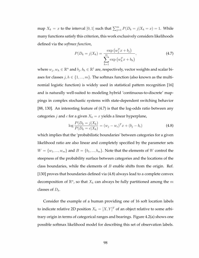
map Xk
= x to the interval [0, 1] such thatP
m
j=1 P (Dk
= j|Xk
= x) = 1. While
many functions satisfy this criterion, this work exclusively considers likelihoods
defined via the softmax function,
P (Dk
= j|Xk
) =
exp
�
wT
j
x+ bj
�
m
X
h=1
exp
�
wT
h
x+ bh
�
, (4.7)
where wj
, wh
2 Rn and bj
, bh
2 R1 are, respectively, vector weights and scalar bi-
ases for classes j, h 2 {1, ...,m}. The softmax function (also known as the multi-
nomial logistic function) is widely used in statistical pattern recognition [16]
and is naturally well-suited to modeling hybrid ‘continuous-to-discrete’ map-
pings in complex stochastic systems with state-dependent switching behavior
[88, 130]. An interesting feature of (4.7) is that the log-odds ratio between any
categories j and c for a given Xk
= x yields a linear hyperplane,
log
P (Dk
= j|Xk
)
P (Dk
= c|Xk
)
= (wj
� wc
)
Tx+ (bj
� bc
) (4.8)
which implies that the ‘probabilistic boundaries’ between categories for a given
likelihood ratio are also linear and completely specified by the parameter sets
W = {w1, ..., wm
} and B = {b1, ..., bm}. Note that the elements of W control the
steepness of the probability surface between categories and the locations of the
class boundaries, while the elements of B enable shifts from the origin. Ref.
[130] proves that boundaries defined via (4.8) always lead to a complete convex
decomposition of Rn, so that Xk
can always be fully partitioned among the m
classes of Dk
.
Consider the example of a human providing one of 16 soft location labels
to indicate relative 2D position Xk
= [X, Y ]
T of an object relative to some arbi-
trary origin in terms of categorical ranges and bearings. Figure 4.2(a) shows one
possible softmax likelihood model for describing this set of observation labels.
98

(a) (b)
Figure 4.2: (a) Probability surfaces for example softmax likelihoodmodel, where class labels take on a discrete range (‘NextTo’,‘Nearby’,‘Far From’) and/or a canonical bearing(‘N’,‘NE’,‘E’,‘SE’,...,‘NW’) (b) Probability surfaces for ex-ample MMS range-only model, where labels with similarrange categories from (a) are treated as subclasses that defineone geometrically convex class (‘Next To’ with s1 = 1) and twonon-convex ones (‘Around’ with s2 = 6 and ‘Far From’ withs3 = 8).
This example shows how the model in (4.8) represents categorical ambiguities
as a function of Xk
: softer weights lead to ‘fuzzier’ probability contours between
class labels, while steeper weights lead to nearly deterministic probabilities over
the geometrically convex regions defining classes. Details on learning W and
B from labeled training data using convex optimization procedures based on
maximum likelihood or maximum a posteriori estimation can be found in [16].
Note that geometric equality constraints can also be imposed on W and B to
enforce desired symmetry, regularity, similarity or congruency conditions for
the underlying class boundary geometries defined via (4.8); such constraints
can substantially reduce the number of parameters to be estimated, which is
particularly useful when learning from sparse human data sets.
99

Extended Softmax Likelihoods
Eq. (4.7) can be generalized by introducing hidden variables to induce non-
convex/multimodal categorical partitions of Xk
. One such generalization is
the multimodal softmax (MMS) model [2], which represents each observable class
j 2 {1, ...,m} as a collection of sj
hidden subclasses dependent on Xk
that are
mutually exclusive and exhaustive, where sj
� 1 andP
m
j=1 sj = S is the total
number of subclasses. Let R represent the hidden subclass variable, which can
take values r 2 {1, ..., S}4, and define Dk
to be conditionally independent of Xk
given R, so that P (Dk
= j, R = r|Xk
) = P (Dk
= j|R = r)P (R = r|Xk
). Further-
more, define �(j) to be the set of all sj
subclasses of class j, where �(j)T
�(c) = ;for j 6= c. If P (D
k
= j|R = r) = I(h 2 �(j)) (the indicator function) and
P (R = r|Xk
) is defined via the softmax model,
P (R = r|Xk
) =
exp
�
wT
h
x+ bh
�
S
X
c=1
exp
�
wT
c
x+ bc
�
, (4.9)
then marginalization of R from P (Dk
= j, R|Xk
) gives
P (Dk
= j|Xk
) =
S
X
r=1
P (Dk
= j, R = r|Xk
) =
S
X
r=1
P (Dk
= j|R = r)P (R = r|Xk
)
=
S
X
r=1
I(r 2 �(j)) · exp
�
wT
c
x+ bc
�
S
X
v=1
exp
�
wT
v
x+ bv
�
=
X
r2�(j)
exp
�
wT
r
x+ br
�
S
X
c=1
exp
�
wT
c
x+ bc
�
.
(4.10)
Hence, the MMS likelihood for Dk
= j given Xk
is the sum of all sj
subclass
softmax likelihoods associated with class j. Given an appropriate subclass con-
figuration [s1, ..., sm], (4.10) can model an arbitrary continuous-to-discrete like-
lihood function using an embedded softmax model to produce piecewise linear4assume without loss of generality that the subclasses are indexed sequentially in class order
100

class boundaries. Figure 4.2 (b) shows a simple example of an MMS model de-
rived from the basic softmax model in Figure 4.2 (a). In this example, the MMS
subclass weights are directly obtained from the model in Figure 4.2 (a), as any
basic softmax model can be trivially converted to an MMS model. However,
it is also generally possible to estimate MMS model parameters directly from
training data when a basic softmax model is unavailable, as discussed in [2, 4]
(geometric constraints can again be easily enforced).
4.2.3 Hybrid Bayesian Inference for Soft Data Fusion
Hybrid Bayesian fusion requires evaluating (4.6) for the continuous prior pdf
p(Xk
) and continuous-to-discrete likelihood P (Dk
= j|Xk
). Although softmax-
based functions are well-suited to modeling P (Dk
= j|Xk
), they unfortunately
do not lead to closed form posteriors p(Xk
|Dk
= j) for any choice of p(Xk
). For
instance, substituting (4.7) into (4.6) for any p(Xk
) yields
p(Xk
|Dk
= j) =1
C· p(X
k
)
exp
�
wT
j
x+ bj
�
m
X
h=1
exp
�
wT
h
x+ bh
�
, (4.11)
where C =
Z 1
�1p(X
k
)
exp
�
wT
j
x+ bj
�
m
X
h=1
exp
�
wT
h
x+ bh
�
dX. (4.12)
Eq. (4.11) cannot be represented in closed form since the integral for the nor-
malization constant C has no analytical solution for any p(Xk
). Furthermore,
even when p(Xk
) is a well-behaved pdf such as a uniform or Gaussian pdf, the
softmax denominator in (4.11) cannot be ‘absorbed’ along with the numerator
and prior into a known parametric family (e.g. the exponential family). There-
fore, (4.6) must be approximated, as in all hybrid Bayesian inference problems
101

involving continuous-to-discrete dependencies [88].
Conventional EKFs or UKF measurement updates (which assume continu-
ous ⇣k
) are not directly applicable to (4.6) due to the hybrid nature of P (Dk
=
j|Xk
). Alternative approximations for such hybrid inference problems are typi-
cally sought using grid-based estimators [21, 131] or Monte Carlo particle filters
[131, 8, 118]. Grid-based methods naturally support recursive Bayesian estima-
tion with arbitary priors and likelihoods, although they scale poorly with state
dimension n, do not provide a compact representation of the posterior, and are
not easily fused with conventional filters for ⇣k
data (e.g. EKFs/UKFs). Particle
approximations are more flexible and easily fused with conventional filters, but
generally do not provide a compact posterior estimate that scales well with n.
In principle, a particle approximation of (4.6) could be compressed into a sin-
gle Gaussian pdf, as in the Gaussian particle filter [83]. However, this leads to
significant information loss when (4.6) is highly non-Gaussian or multimodal.
Online global compression of particles to more flexible Gaussian mixture pdfs
is also possible [83, 45], but the required learning methods are prone to poor
local solutions and can be computationally demanding. Furthermore, sampling
approximations require special care to ensure accuracy and to mitigate undesir-
able phenomena such as sample degeneracy. For instance, the performance of
the standard bootstrap particle filter [8] can degrade significantly if n is large
and/or if the observation likelihood is small [115].
Motivated by the success of principled Gaussian/Gaussian mixture (GM)
posterior estimates for conventional ⇣k
fusion [6, 45], this paper develops prin-
cipled Gaussian/GM estimates for (4.6) using novel hybrid inference approx-
imations. Gaussian/GM posterior representations are especially desirable for
102

practical human-robot fusion applications since they: (i) have computational
costs that scale well with n and number of categories m, and (ii) can be com-
pactly represented through sufficient statistics, which facilitates online storage,
communication, and fusion with conventional dynamic filters (for ⇣k
). Section
4.3 develops the proposed hybrid inference approximation for the baseline case
of a Gaussian prior p(Xk
) and a basic softmax likelihood P (Dk
= j|Xk
). This
leads to a baseline Gaussian posterior approximation p(Xk
|Dk
= j) via varia-
tional Bayesian importance sampling (VBIS) for accurate estimation of (4.6) via
first and second order moments. Section 4.4 then extends this baseline VBIS
approximation to a general GM posterior estimate of (4.6) in the case of a GM
prior with MMS likelihood. The proposed VBIS approximations are guaran-
teed to converge to unique solutions and are easily coupled with conventional
Gaussian/GM-based fusion algorithms for conventional ⇣k
robot sensor data.
4.3 Soft Fusion via Variational Bayes and Importance Sampling
Methods
4.3.1 Baseline Variational Bayes Approximation
Assume that Xk
has a Gaussian prior p(Xk
) = N (µ,⌃) with mean µ 2 Rn
and covariance matrix ⌃ 2 Rn⇥n, and let P (Dk
= j|Xk
) be given by (4.7) for
m � 2. Ref. [100] shows that when m = 2, the joint pdf p(Xk
, Dk
= j) in
(4.6) is well-approximated by an unnormalized Gaussian pdf via the variational
lower bound to the binary logistic function proposed by [66]; this leads to a
variational Bayesian (VB) Gaussian posterior approximation p(Xk
|Dk
= j) upon
103

renormalization. While this approach leads to an efficient and close approxi-
mation to the true posterior, it is limited to logistic likelihoods P (Dk
= j|Xk
)
or to tree-based hierarchical models defined strictly through the binary logistic
function (e.g. see [17]), which are cumbersome and difficult to learn/specify
when m > 2. The VB Gaussian approximation strategy is generalized here for
m � 2 via the basic softmax likelihood (4.7), which gives more flexible and eas-
ily specifiable/learnable human likelihood models.
Defining f(Dk
= j,Xk
) for now to be an unnormalized Gaussian function
that approximates the softmax likelihood P (Dk
= j|Xk
), the joint pdf and nor-
malization constant (4.12) are approximated as
p(Xk
, Dk
= j) ⇡ p(Xk
, Dk
= j) = p(Xk
)f(Dk
= j,Xk
), (4.13)
C ⇡ ˆC =
Z 1
�1p(X
k
, Dk
= j)dXk
. (4.14)
Note that p(Xk
, Dk
= j) is an unnormalized Gaussian, since the product of any
two Gaussians is generally an unnormalized Gaussian [5]. This permits ˆC to be
evaluated in closed form as an approximation to the marginal likelihood of the
discrete observation, C = P (Dk
= j), in (4.6).
For m � 2, f(Dk
= j,Xk
) is derived here via the upper bound to the prob-
lematic softmax denominator in (4.7) that was proposed by [20], which uses a
variational product of m unnormalized Gaussians. Specifically, for any set of
scalars ↵, ⇠c
and yc
for c 2 {1, ...,m}, [20] proves that
log
m
X
c=1
eyc
!
↵ +
m
X
c=1
yc
� ↵� ⇠c
2
+ �(⇠c
)[(yc
� ↵)2 � ⇠2c
] + log(1 + e⇠c),
(4.15)
where �(⇠c
) =
1
2⇠c
1
1 + e�⇠c� 1
2
�
and yc
= wT
c
x+ bc
. (4.16)
The variables ↵ and ⇠c
are free variational parameters; given yc
, ↵ and ⇠c
are se-
lected to minimize the upper bound in (4.15), thus providing the tightest pos-
104

sible upper-bounding approximation to the denominator of (4.7). Assume for
now that these ↵ and ⇠c
are known; the procedure for selecting ↵ and ⇠c
is given
in Sec. 4.3.1. Now, from (4.7), it follows that
logP (Dk
= j|Xk
) = wT
j
x+ bj
� log
m
X
c=1
ewTc x+bc
!
. (4.17)
After replacing the second term on the right-hand side with the bound in (4.15),
subsequent simplification gives
f(Dk
= j,Xk
) = exp(gj
+ hT
j
x� 1
2
xTKj
x), (4.18)
where gj
=
1
2
"
bj
�X
c 6=j
bc
#
+ ↵(m
2
� 1)
+
m
X
c=1
⇠c
2
+ �(⇠c
)[⇠2c
� (bc
� ↵)2]� log(1 + e⇠c), (4.19)
hj
=
1
2
"
wj
�X
c 6=j
wc
#
+ 2
m
X
c=1
�(⇠c
)(↵� bc
)wc
, (4.20)
Kj
= 2
m
X
c=1
�(⇠c
)wc
wT
c
, (4.21)
and where f(Dk
= j,Xk
) P (Dk
= j|Xk
) follows from (4.15). Since the prior
can also be expressed as
p(Xk
) = exp(gp
+ hT
p
x� 1
2
xTKp
x), (4.22)
where gp
= �1
2
(log |2⇡⌃|+ µTKp
µ), hp
= Kp
µ, Kp
= ⌃
�1, (4.23)
substitution of (4.22) and (4.18) into (4.13) gives the unnormalized Gaussian
joint pdf approximation,
p(Xk
, Dk
= j) = exp(gl
+ hT
l
x� 1
2
xTKl
x), (4.24)
where gl
= gp
+ gj
, hl
= hp
+ hj
, Kl
= Kp
+Kj
. (4.25)
Normalization of (4.24) gives the desired variational Gaussian posterior pdf
approximation for m � 2,
p(Xk
|Dk
= j) = N (µ, ˆ⌃), (4.26)
105

where ˆ
⌃VB = K�1l
, µVB = K�1l
hl
. (4.27)
The approximate posterior mean and covariance updates in (4.27) for discrete
measurements bear close resemblance to the corresponding continuous mea-
surement updates for the Kalman information filter [10]. With this resemblance
in mind, an examination of Kj
and hj
in (4.21) suggests that the softmax weight
vectors wj
determine the ‘average information’ content about Xk
contained in
each category j. This is intuitively reasonable: as shown in Fig. 4.2, large
magnitude weights indicate sharp log-odds boundaries between classes in eq.
(4.8) (i.e. less ambiguity and greater separability between discrete classes as a
function of Xk
), which leads to more informative updates for Xk
since p(Xk
)
is ‘squashed’ more strongly by P (Dk
= j|Xk
) via (4.6). On the other hand,
smaller magnitude weights imply that the log-odds boundaries between classes
are less well-defined (i.e. classes are less distinct from each other as a function
of Xk
), so that the prior is squashed less by the likelihood via (4.6). Finally, note
that ˆ
⌃VB is independent of the actual discrete observation Dk
= j, just as co-
variance/information matrix updates for the Kalman filter are independent of
observed continuous measurements.
Variational Parameter Optimization
Analytical minimization of the right-hand side of (4.15) with respect to the free
variational parameters ↵ and ⇠c
gives
⇠2c
= y2c
+ ↵2 � 2↵yc
, (4.28)
↵ =
�
m�24
�
+
P
m
c=1 �(⇠c)ycP
m
c=1 �(⇠c). (4.29)
However, these formulas cannot be used to compute (4.26) directly since yc
depends on Xk
, which is unobserved. Therefore, following the same strategy as
106

[100] for the m = 2 case, the variational parameters are chosen to minimize the
expected value of (4.15) with respect to the posterior. It is straightforward to show
that this is equivalent to maximizing the approximate marginal log-likelihood of
the observation Dk
= j,
log
ˆC = log
Z 1
�1p(X
k
, Dk
= j)dXk
, (4.30)
where log
ˆC logC. Eq. (4.30) can be expressed in closed-form via standard
Gaussian identities, but direct maximization of (4.30) with respect to ↵ and ⇠c
involves cumbersome calculation of highly non-linear gradient and Hessian
terms. The expectation-maximization (EM) algorithm [16] can instead be in-
voked to iteratively optimize ↵ and ⇠c
via expected values of (4.28) and (4.29),
while alternately updating p(Xk
|Dk
= j) via simple closed-form expressions.
The EM procedure is given in Algorithm 1, where the yc
terms in (4.28) and
(4.29) are replaced by their expected values under the current p(Xk
|Dk
= j)
estimate at each E-step,
hyc
i = wT
c
µ+ bc
, (4.31)⌦
y2c
↵
= wT
c
⇣
ˆ
⌃VB + µVBµT
VB
⌘
wc
+ 2wT
c
µVBbc + b2c
. (4.32)
Since (4.28) and (4.29) are non-linearly coupled, an iterative resubstitution loop
is required for convergence of ⇠c
and ↵ (15 iterations were sufficient for this
paper’s implementations).
As shown in the Appendix, p(Xk
|Dk
= j) is log-concave, which implies that
the baseline Gaussian-softmax posterior is always unimodal. Hence, Algorithm
1 satisfies the necessary and sufficient condition derived in [122] to guarantee
monotonic convergence to a unique set of variational parameters for the local
VB lower bound Gaussian approximation. Convergence can be gauged by eval-
107

uating the change in (4.30) after each M-step, where
log
ˆC = hyj
i � ↵
+
m
X
c=1
⇢
1
2
(↵ + ⇠c
� hyc
i)� �(⇠c
)[
⌦
y2c
↵� 2↵ hyc
i+ ↵2 � ⇠2c
]� log(1 + e⇠c)
�
� 1
2
0
@
log
|⌃|�
�
�
ˆ
⌃VB
�
�
�
+ tr(⌃�1ˆ
⌃VB) + (µ� µVB)T
⌃
�1(µ� µVB)� n
1
A (4.33)
and most of the required terms are already used in the E and M steps. However,
it is often more convenient to monitor convergence of µVB between iterations, so
that the lower bound (4.33) can be evaluated at the end, if desired.
Algorithm 1: Local Variational Bayes EM Update
Input: prior µ and ⌃; Dk
= j with likelihood in eq.(4.7), initial ↵ and ⇠c
, for
j, c 2 {1, ...,m}Output: posterior mean µVB and covariance ˆ
⌃VB
1. E-step: for all fixed ⇠c
and ↵,
(a) compute µVB and ˆ
⌃VB via eq. (4.27);
(b) compute hyc
i and hy2c
i via eqs. (4.31)-(4.32);
2. M-step: for all fixed hyc
i and hy2c
i,for i = 1 : n
lc
do
(a) compute all ⇠c
for fixed ↵ via eq. (4.28)
(b) compute ↵ for all fixed ⇠c
via eq. (4.29)
end for
3. If converged, return ˆC via eq. (4.33) and stop; otherwise, return to step 1.
108

4.3.2 Improved Baseline VB Approximation with Importance
Sampling
Understanding the consequences of using the Gaussian variational lower bound
(4.18) in place of the true softmax likelihood P (Dk
= j|Xk
) is important. Con-
sider Fig. 4.3, which shows the variational lower bound approximation and re-
sulting posterior for a standard normal prior and two different binary softmax
likelihoods in 1D. Fig. 4.3 (a) and (b) show that (4.24) is generally a close lower
bound approximation of the true joint pdf; as shown in Fig. 4.3 (c) and (d), a
key benefit of this property of the VB approximation is that µVB closely approx-
imates the true mean of (4.6) upon renormalization. However, Fig. 4.3 (c) and
(d) also show that since ˆC C, the approximate posterior (4.26) obtained from
dividing (4.24) by ˆC no longer lower bounds the true posterior p(Xk
|Dk
= j).
In fact, even if p(Xk
, Dk
= j) and p(Xk
, Dk
= j) are quite similar, multiplication
of (4.24) by ˆC�1 � C�1 forces (4.26) to be more concentrated around the peak
than 4.6, and therefore ˆ
⌃VB is optimistic relative to the true posterior covariance
5. The benefits of a good estimate in µVB, can be outweighed by such optimism
in the ˆ
⌃VB estimate, since this can lead to severe overconfidence and inconsisten-
cies during recursive Bayesian fusion. Optimism in ˆ
⌃VB also tends to produce
a very small bias in µVB relative to the true posterior mean, as the approximate
posterior sufficient statistics are linked via (4.27).
As an alternative augmentation, the characteristic that µVB from VB is close
to the true mean of the unimodal posterior can be exploited by another fast
estimation procedure to significantly improve the estimates of µVB and ˆ
⌃VB in
(4.26). Monte Carlo importance sampling (IS) [91] is particularly well-suited to
5i.e. (⌃true post � ⌃VB) will be positive semi-definite
109

(a) (b)
(c) (d)
Figure 4.3: Bayesian update example for standard normal Gaussian prior(green) and binary softmax likelihood (blue), showing trueposterior (magenta), softmax lower bound (black dash), andapproximate joint pdf (red dash) for (a) soft softmax weights,with C = 0.1555 and ˆC = 0.1525 and (b) steep softmax weights,with C = 0.4220 and ˆC = 0.2460. True posterior and approxi-mate VB Gaussian posterior for cases (a)-(b) are shown in (c)-(d), respectively.
this end, since it quickly can evaluate arbitrary moments of (4.6) using any ‘im-
portance distribution’ that roughly corresponds to (4.6). Specifically, given Ns
samples {xi
}Ns
i=1 2 Xk
drawn from an importance density q(Xk
), IS approximates
the expectation of an arbitrary function f(Xk
) with respect to p(Xk
|Dk
= j) as
hf(Xk
)i =Z 1
�1p(X
k
|Dk
= j)f(Xk
)dXk
⇡NsX
i=1
!i
f(xi
), (4.34)
!i
/ p(xi
)P (Dk
= j|xi
)
q(xi
)
, (4.35)
where !i
is the importance weight for sample i, µ = hXk
i and ˆ
⌃ =
110

⌦
(Xk
� µ)(Xk
� µ)T↵
. Note that (4.35) exploits the fact that the target posterior
density p(Xk
|Dk
= j) only needs to be known up to some normalizing constant,
so that the joint pdf p(xi
, Dk
= j) = p(xi
)P (Dk
= j|xi
) can be used to compute
each !i
(as is standard practice in this case, the !i
must be renormalized to sum
up to 1, which introduces a vanishingly small bias into (4.34) [115]). Although
q(Xk
) can in theory be any pdf that is easy to sample from and ensures proper
support coverage of p(Xk
|Dk
= j) (i.e. p(Xk
|Dk
= j) > 0) q(Xk
) > 0), the esti-
mate (4.34) is only reliable for reasonable values of Ns
when q(Xk
) is sufficiently
‘close’ to p(Xk
|Dk
= j).
Since the true posterior is unimodal and has a mean that is close to µVB, it is
natural to specify q(Xk
) as a unimodal pdf whose mean is parameterized by µVB.
The prior covariance ⌃ can also be used to constrain the size/shape of q(Xk
) to
ensure adequate coverage of p(Xk
|Dk
= j). This is justified since the prior, joint
and posterior pdfs are all unimodal, so that conditioning on Dk
= j reduces
the uncertainty in the posterior relative to the prior such that (⌃ � ⌃true post) is
expected to be positive definite [10].
These considerations lead to the Variational Bayesian IS (VBIS) inference al-
gorithm, proposed here as drawing upon the strengths of both VB and IS. An
outline of the VBIS procedure is shown in Algorithm 2. The VB estimate in
Algorithm 1 is first used to define q(Xk
), which is then applied to (4.34) to es-
timate µVBIS and ˆ
⌃VBIS for the Gaussian posterior approximation p(Xk
, Dk
= j) =
N (µVBIS, ˆ⌃VBIS). This work uses
q(Xk
) = N (µVB,⌃), (4.36)
since this pdf is straightforward to sample from and permits convenient cal-
culation of !i
. Other, more sophisticated unimodal pdfs could serve as q(Xk
)
111

on the basis of µV B
and ⌃ (e.g. heavy-tailed Laplace pdfs or mixture model
pdfs). However, compared with (4.36), the benefits of such alternatives are of-
ten outweighed by the extra computational cost of sampling xi
and evaluating
!i
, especially if n � 2 (e.g. an n-dimensional Laplace pdf with covariance ⌃
requires Bessell functions to evaluate !i
[49]).
4.3.3 Likelihood weighted importance sampling (LWIS)
Another possible importane sampling strategy for computing µ and ˆ
⌃ is to by-
pass VB altogether in Algorithm 2 and simply set q(Xk
) = p(Xk
), so that (4.35)
becomes !i
/ P (Dk
= j|xi
). This approach, popularly known as likelihood
weighted importance sampling (LWIS) [123, 88], defines the measurement update
step of the standard bootstrap particle filter [8] and works well if p(Xk
) and
p(Xk
|Dk
= j) are similar. While faster and nominally more computationally
convenient than VBIS, LWIS suffers if Dk
= j is ‘surprising’ with respect to
p(Xk
) (i.e. the prior and posterior are not close) or if P (Dk
= j|Xk
) is highly
peaked relative to p(Xk
) [30]. In such cases, !i
= 0 for many samples, leading to
inconsistent LWIS estimates. LWIS is presented here as a common benchmark
algorithm for estimating complex non-Gaussian densities.
4.3.4 Numerical 1D Example
Fig. 4.4 (a) gives a hypothetical 1D softmax likelihood model for a human ob-
servation Dk
, with m = 5 categories relating to Xk
, the location of a static target
relative to a robot. The prior p(Xk
) at some fixed time step k is shown in gray
112

Algorithm 2: VBIS Measurement Update
Input: prior µ and ⌃; D = j with likelihood in eq.(4.7), initial ↵ and ⇠c
, for
j, c 2 {1, ...,m}Output: posterior mean µVBIS and covariance ˆ
⌃VBIS
1. Obtain initial estimates µV B
and ˆ
⌃
V B
using local VB EM update (Algorithm
1)
2. Importance sampling correction:
a. set q(Xk
) = N (µV B
,⌃)
b. draw Ns
samples {xi
}Ns
i=1 from q(Xk
)
c. compute importance weights {!i
}Ns
i=1 using (4.35) and normalize so thatP
Ns
i=1 !i
= 1
d. re-estimate posterior mean and covariance,
µVBIS =
NsX
i=1
!i
xi
, ˆ
⌃VBIS =
NsX
i=1
!i
xi
xT
i
� µVBISµVBIS
for three different scenarios in (b)-(d); in this example, the robot does not move
or contribute continuous sensor data ⇣k
, but the update relies solely on a soft
human observation Dk
. Figs. 4.4 (b)-(d) show the most likely soft observation
Dk
= j for j 2 D provided by the human in each case relative to the true target
location xtrue (black star). Moving from (b)-(d), the prior becomes less accurate
(i.e. more surprising/inconsistent) compared to xtrue. Such inconsistencies could
arise, for instance, via faulty information obtained from another agent or an
inaccurate/highly uncertain dynamics model.
Fusion results are shown for exact numerical integration (magenta), VB
(red), VBIS with Ns
= 200 samples (dark green, five sample results shown), and
113

!10 !8 !6 !4 !2 0 2 4 6 8 100
0.2
0.4
0.6
0.8
1
Target displacement from robot, Xk (m)
Like
lihoo
d V
alue
, P(D
k=j |
Xk)
Categorical Softmax Likelihoods for Dk
P(Dk = Far West | Xk)
P(Dk = Near West | Xk)
P(Dk = Next To | Xk)
P(Dk = Near East | Xk)
P(Dk = Far East | Xk)
!10 !8 !6 !4 !2 0 2 4 6 8 100
0.2
0.4
0.6
0.8
1
Results for Dk = Near West , Prior at µ = !1.5, s2 = 1
Target displacement from robot, Xk (m)
PD
F va
lue
p(Xk) (prior)
Exact p(Xk | Dk)
VB p(Xk | D)
Typical LWIS p(Xk | Dk)
Typical VBIS p(Xk | Dk)
True Target Location
(a) (b)
−10 −8 −6 −4 −2 0 2 4 6 8 100
0.2
0.4
0.6
0.8
1
Results for Dk = Next To, Prior at µ = −8, !2 = 4
Target displacement from robot, Xk (m)
PD
F va
lue
p(Xk) (prior)
Exact p(Xk | Dk)
VB p(Xk | D)
Typical LWIS p(Xk | Dk)
Typical VBIS p(Xk | Dk)
True Target Location
!10 !8 !6 !4 !2 0 2 4 6 8 100
0.2
0.4
0.6
0.8
1
Results for Dk = Near East, Prior at µ = !8, s2 = 4
Target displacement from robot, Xk (m)
PD
F va
lue
p(Xk) (prior)
Exact p(Xk | Dk)
VB p(Xk | D)
Typical LWIS p(Xk | Dk)
Typical VBIS p(Xk | Dk)
True Target Location
(c) (d)
Figure 4.4: Synthetic 1D fusion problem using exact and approximate in-ference methods: (a) human observation softmax likelihoodcurves for P (D
k
= j|Xk
), (b)-(d) posterior approximation re-sults for human observations that are progressively more sur-prising relative to p(X
k
) (five sample posterior results shownfor LWIS and VBIS Gaussian approximations in each case).
LWIS with Ns
= 200 samples (blue, 5 typical results shown). The true mean and
variance (µ⇤, �2⇤) of the exact (non-Gaussian) posterior are shown in Table 4.1,
along with the corresponding estimates and MATLAB computation times for
each approximate method over 50 different trials. The number of EM iterations
for VB and VBIS are also shown 6. The effective sample size (ESS) is also provided
6using a random initial guess for ↵ in (4.29) and a tolerance of 1e-3 on C
114

Table 4.1: Results for 1D Fusion Problem in Figure 4.4
Case µ⇤ , �2⇤ µ
V B
, �2V B
µV BIS
, �2V BIS
µLWIS
, �2LWIS
VB time, EM steps IS time, VB/LW ESS
b -2.56, 0.48 -2.55, 0.195 -2.55 ± 0.04, 0.49 ± 0.04 -2.55±0.07, 0.68±0.07 11.6 ms, 12 1 ms, 167, 91.7
c -2.34, 0.84 -2.27, 0.236 -2.32 ± 0.06, 0.85 ± 0.08 -2.90±0.84, 0.53±0.15 13.8 ms, 16 1 ms, 115, 22
d 0.993, 1.28 1.02, 0.259 1.01 ± 0.07, 1.28 ± 0.11 -2.62±0.90, 0.15±0.05 10.6 ms, 10 1 ms, 141, 16.7
as a measure sampling effiency for VBIS and LWIS, where ESS(Ns
) =
Ns1+cv
2(z)
and cv2(z) is the coefficient of variation for the unnormalized importance weights
!i
. ESS estimates the number of samples that are effectively contributing to the
estimate and thus indicates the ‘closeness’ of q(Xk
) to p(Xk
|Dk
= j) (a low ESS
indicates an unreliable estimate) [91].
In all scenarios, µVB is very close to µ⇤ with a small bias, while �2VB always
underestimates �2⇤ in each case. The posterior mean and variance approxima-
tions are quite accurate for both VBIS and LWIS in (b), since Dk
is unsurprising
with respect to p(Xk
). However, since p(Xk
) and Dk
disagree more in (c)-(d),
the LWIS Gaussian posterior approximation becomes steadily worse in these
cases, whereas VBIS always maintains a fairly close Gaussian approximation
with only 200 samples. The poor performance of LWIS in (c) and (d) is re-
flected by its diminishing ESS and the erratic/inconsistent nature of µLWIS and
�2LWIS. LWIS can be improved in (c) and (d) by increasing N
s
, although this has
limited impact in (d): setting Ns
= 10, 000 matches the computation time for
VBIS but still yields worse performance (ESS=200, µLWIS = �0.70 ± 0.75 and
�2LWIS = 0.47±0.08) than the VBIS with N
s
= 200. Note that the computation time
for VBIS here is modest: using unoptimized MATLAB code, VB requires 10-14
ms (10-16 EM iterations) to converge, while IS only requires 1 ms for Ns
= 200.
115

4.4 Soft Fusion with Non-Gaussian Priors and Multimodal
Likelihoods
VBIS nominally assumes that p(Xk
) is Gaussian and that P (Dk
= j|Xk
) is a
basic softmax likelihood (4.7) with convexly separable classes. However, these
assumptions are often violated in practical human-robot fusion scenarios. The
prior p(Xk
) can be non-Gaussian through initial beliefs (e.g. uniform or mul-
timodal priors on target location), if Xk
evolves with non-Gaussian/nonlinear
dynamics (e.g. unobservable dynamic mode changes for moving targets), or if
updates via ⇣k
in Fig. 4.1 involve highly non-Gaussian sensor likelihoods (e.g.
detector readings from cameras [21, 118]). Furthermore, a number of situations
arise where (4.7) is inadequate for modeling P (Dk
= j|Xk
). For instance, soft
range-only observations induce non-convex categorizations of Xk
that are bet-
ter modeled by extended likelihood models such as MMS (cf. Section 2). Fortu-
nately, VBIS can be extended for recursive Bayesian information fusion in such
scenarios using Gaussian mixture (GM) pdf approximations.
In the sequel, it is assumed that the prior p(Xk
) in (4.6) is given by an M -term
GM,
p(Xk
) =
M
X
u=1
p(u,Xk
) =
M
X
u=1
P (u) · p(Xk
|u) =M
X
u=1
cu
· N (µu
,⌃u
), (4.37)
where the hidden discrete component index variable U takes values u 2{1, ...,M}, µ
u
2 Rn and ⌃u
2 Rn⇥n are respectively the uth component mean and
covariance, and the component index weights cu
2 R satisfyP
M
u=1 cu = 1. Since
GMs can approximate any pdf arbitrarily well through the compact M -mixand
parameter set {µu
,⌃u
, cu
}Mu=1, they are well-suited to Bayesian information fu-
sion problems involving complex pdfs. The universal approximation prop-
116

erty of GMs was exploited by [6] to derive recursive nonlinear/non-Gaussian
Bayesian state estimators for continuous measurements via parallel banks of
KFs/EKFs, whose outputs are combined to form a single GM posterior approx-
imation at each time step. This approach was later extended to incorporate GM
approximations via parallel banks of UKFs and PFs in [45] and [83], respectively.
Due to their beneficial statistical properties and high flexibility, GM-based fu-
sion algorithms have been used in a variety of robotics applications, such as
autonomous localization in urban environments [120] and cooperative target
tracking with decentralized agents [76]. For the purposes of this paper, any
GM-based ⇣k
fusion algorithm (i.e. a Gauss sum filter derived via EKFs, UKFs,
PFs, etc.) can be used to approximate eq. (4.1) or (4.2) as the prior pdf (4.37) for
soft human data fusion. Furthermore, it is assumed that the extended softmax
likelihood P (Dk
= j|Xk
) is given by the MMS model in eq. (4.10).
4.4.1 VBIS with GM priors and MMS likelihoods
An approximation to p(Xk
|Dk
= j) is derived by first considering the joint pdf
given Dk
= j,
p(Dk
= j,Xk
, U, R) = P (Dk
= j, R|Xk
, U)p(Xk
, U)
= P (Dk
= j, R|Xk
)p(Xk
, U) = P (Dk
= j|R)P (R|Xk
)p(Xk
|U)P (U), (4.38)
where the first line follows from Bayes’ rule and the second line follows
from the conditional indepedence properties of the MMS model (cf. Section
2). Recall from Section 2 that: (i) R is a hidden subclass variable with values
r 2 {1, ..., S}, where each subclass is deterministically mapped to a single class
label j 2 {1, ...,m} for the observation Dk
, and (ii) �(j) denotes the set of sj
sub-
classes mapping to j, where P (Dk
= j|r) = I(r 2 �(j)). From the law of total
117

probability, the posterior p(Xk
|Dk
= j) can therefore be expressed as
p(Xk
|Dk
= j) =
M
X
u=1
X
r2�(j)
p(Xk
|u, r,Dk
= j)P (u, r|Dk
= j). (4.39)
In other words, the posterior can be expressed as a mixture of conditional pos-
teriors for all possible valid joint configurations (u, r 2 �(j)) of the hidden vari-
ables given Dk
= j. Using Bayes’ rule and the joint pdf (4.38), the first term in
the summand of (4.39) can be written as
p(Xk
|Dk
= j, u, r) =P (D
k
= j|r)P (r|Xk
)p(Xk
|u)P (u)R
P (Dk
= j|r)P (r|Xk
)p(Xk
|u)P (u)dXk
. (4.40)
Cancelling the terms independent of Xk
gives
p(Xk
|Dk
= j, u, r) =P (r|X
k
)p(Xk
|u)R
P (r|Xk
)p(Xk
|u)dXk
, (4.41)
which is the conditional posterior of Xk
given observation Dk
= j, mixing com-
ponent u, and subclass r 2 �(j). Note that (4.41) is equivalent to the baseline
posterior in eq. (4.11): the numerator in (4.41) is the product of a Gaussian com-
ponent p(Xk
|u) = N (µu
,⌃u
) and a softmax likelihood P (r|Xk
), while the de-
nominator is the marginal softmax observation likelihood of subclass r 2 �(j)
under Gaussian component u. Therefore, (4.41) is a unimodal conditional pdf
that can be well-approximated by a Gaussian using the VBIS procedure in Al-
gorithm 2, so that
p(Xk
|Dk
= j, u, r) ⇡ p(Xk
|Dk
= j, u, r) = N (µzr
, ˆ⌃zr
). (4.42)
Next, the second summand in (4.39) P (r, u|Dk
= j) can be written as
P (r, u|Dk
= j) =P (r, u,D
k
= j)
P (j)(4.43)
=
P (r, u,Dk
= j)P
M
u=1
P
r2�(j) P (r, u,Dk
= j)=
1
CP (r, u,D
k
= j), (4.44)
where the numerator can be derived from (4.38) as
P (r, u,Dk
= j) =
Z
p(Xk
|u)P (r|Xk
)P (Dk
= j|r)P (u)dXk
118

= P (u)
Z
p(Xk
|u)P (r|Xk
)dXk
, (4.45)
where P (u) = cu
from (4.37) and the last line follows from P (Dk
= j|r) = 1 for
r 2 �(j), from the definition of the MMS model. Note that the integral in (4.45)
is the same as the denominator in (4.41), i.e. the marginal softmax observation
likelihood of subclass r under component u,
P (r|u) =Z
p(Xk
|u)P (r|Xk
)dXk
= Cru
. (4.46)
Substituting these expressions into (4.45) and then (4.44) gives
P (r, u|Dk
= j) =1
C· c
u
· Cru
(4.47)
Eq. (4.46) is analytically intractable, but can be estimated in two ways. Firstly,
since VBIS is used to estimate (4.41) through Algorithm 2, (4.46) can be directly
approximated by a corresponding variational likelihood lower bound ˆCru
Cru
obtained via (4.33) in Algorithm 1. In this case, the nominal conditioning on
Dk
= j in (4.33) is replaced by conditioning on R = r and U = u, so that
individual µru
, ˆ⌃rz
, ⇠c,ru
, and ↵ru
estimates are used in (4.33) for each possible r
and u pairing to compute log
ˆCru
. However, since Cr,u
is always underestimated
by the lower bound ˆCru
, this approach could bias the posterior approximation
when the bound is insufficiently tight. Alternatively, (4.46) can be estimated via
direct sampling as
ˆPs
(r|u) = 1
Nu
NuX
l=1
P (r|Xk
= xl
), (4.48)
where {xl
}Nu
l=1 is a set of Nu
samples drawn directly from the uth prior compo-
nent N (µu
,⌃u
). However, the variance of ˆPs
(r|u) is inversely proportional to
P (r|u) and Nu
, meaning that (4.48) can fall below the lower bound ˆCru
if P (r|u)is very small (i.e. P (r|u) << 0.01) and N
u
is insufficiently large. Therefore,
to obtain a reasonable estimate for a given Nu
, ˆCru
is used to floor (4.48) as a
119

consistency check. Thus, (4.46) is estimated as
P (r|u) ⇡ max[exp(
ˆCru
), ˆPs
(r|u)] ⌘ ˆP (r|u). (4.49)
Hence, eq. (4.47) becomes
P (r, u|Dk
= j) ⇡ 1
˜C· c
u
· ˆP (r|u) ⌘ ˆ�ru
, (4.50)
where ˜C =
M
X
u=1
X
r2�(j)
cu
· ˆP (r|u). (4.51)
Finally, combining (4.41) and (4.51) into (4.39) yields a GM posterior approxi-
mation to p(Xk
|Dk
= j),
p(Xk
|Dk
= j) ⇡ p(Xk
|Dk
= j) (4.52)
=
M
X
u=1
X
r2�(j)
ˆ�ru
· N (µru
, ˆ⌃ru
) =
K
X
h=1
ˆ�h
· N (µh
, ˆ⌃h
) (4.53)
with K = sj
·M components.
4.4.2 LWIS fusion and VB-only fusion for GM priors and MMS
likelihoods
Algorithm 3 summarizes the generalized VBIS fusion algorithm for GM priors
and MMS likelihoods. Note that, if the VBIS Gaussian approximation in step 4
of Algorithm 3 is replaced by an LWIS Gaussian approximation for component
h and ˆP (r|u) =
ˆPs
(r|u) is instead used in step 5, an LWIS-based GM approx-
imation to the posterior (4.39) is obtained. Likewise, a VB-only GM posterior
approximation can be obtained by using only Algorithm 1 in step 4 (i.e. ignor-
ing the IS correction) and by setting ˆP (r|u) =
ˆCru
in step 5 (i.e. ignoring step
3). The next example shows that the VBIS procedure in Algorithm 3 improves
considerably on both of these alternative methods. Note that the VB, VBIS, and
120

LWIS baseline Gaussian posterior approximations given in Section 4.3 for Gaus-
sian priors and softmax likelihoods are special cases of the corresponding GM
posterior approximations for GM priors and MMS likelihoods, with M = 1 and
sj
= 1 8j 2 {1, ...,m}.
Algorithm 3: VBIS for GMs and MMS likelihoods
Input: M -component prior GM with pdf in eq. (4.37) and sufficient statistics
{µu
,⌃u
, cu
}Mu=1; observation D
k
= j with likelihood in eq.(4.10) and sj
relevant
subclasses in set �(j)
Output: posterior GM with pdf in eq. (4.53) and sufficient statisticsn
µh
, ˆ⌃h
, ˆ�h
o
M ·sj
h=1
1. set h = 0
for each relevant subclass r 2 �(j) do
for u = 1 : M do
2. set h = h+ 1
3. compute ˆPs
(r|u) via eq. (4.48) using Nu
samples {xl
}Nu
l=1 drawn from
N (µu
,⌃u
)
4. obtain (µh
, ˆ⌃h
, ˆCh
) from VBIS fusion (Algorithm 2) using Ns
samples,
µ = µu
, ⌃ = ⌃
u
and Dk
= r
5. compute ˆP (r|u) = max[exp(
ˆCh
), ˆPs
(r|u)]6. set ˆ�
h
= cu
· ˆP (r|u)end for
end for
7. renormalize all ˆ�h
such thatP
M ·sjh=1
ˆ�h
= 1
121

Numerical 1D Example
Figure 4.5 modifies the previous 1D human-robot fusion example in Fig. 4.4,
so that p(Xk
) is now an M = 4 component GM (gray) and Dk
now takes the
form of a coarse range observation with m = 3 non-convex categories: ‘Next
To’, ‘Nearby’, and ‘Far From’. The corresponding MMS likelihood model is
shown in Fig. 4.5 (a). Note the multimodality of both p(Xk
) and the likeli-
hood model; Figure 4.5 (b) shows the results of fusing the surprising observa-
tion Dk
= ‘Far From’ via numerical integration to obtain the exact multimodal
posterior pdf (magenta). Also shown are the full 8-component GM posterior
approximations obtained with 100 trials of VBIS using Nu
= Ns
= 500 (Alg. 3,
dark green), 100 trials of LWIS using 500 samples (blue), and VB-only (red).
Fig. 4.5 (b) shows that LWIS barely captures the minor posterior modes on
the right and struggles to approximate the major posterior modes on the left.
This behavior is again due to the brittleness of LWIS to surprising measure-
ments. The VB-only GM approximation (which required 11-23 EM steps per
component for a total of 131 steps) shows considerable improvement in approx-
imating the posterior modes, but it still significantly underestimates all compo-
nent variances as well as the largest component weight on the left. In constrast,
VBIS provides a very high-fidelity GM approximation to the exact posterior us-
ing 500 samples and less than 20 EM iterations per posterior component. Table
4.2 shows the resulting computation times (using unoptimized Matlab code)
and Kullback-Leibler divergences (KLDs) between the true posterior p(Xk
|Dk
)
(from numerical integration) and each GM approximation p(Xk
|Dk
), where the
122

KLD is given by
KL[p(Xk
|Dk
)||p(Xk
|Dk
)] =
Z
p(Xk
|Dk
) log
✓
p(Xk
|Dk
)
p(Xk
|Dk
)
◆
dXk
. (4.54)
The KLD is a non-negative information theoretic measure of ‘distance’ between
two pdfs, where (4.54) is zero iff p(Xk
|Dk
) = p(Xk
|Dk
). A smaller KLD indicates
that p(Xk
|Dk
) loses less information from p(Xk
|Dk
) and is therefore a better ap-
proximation to the true posterior. Clearly, LWIS loses the most information on
average, while VBIS loses significantly less information than either LWIS or VB-
only. Repeating LWIS with 1500 samples matches the time required for VBIS
with 500 samples, but only reduces the LWIS KLD by about half. Also, the VBIS
KLD increases to 0.23 ± 0.20 if the direct-sampling estimate ˆPs
(r|u) of Cru
is only
used in step 5 of Algorithm 3 (i.e. if the likelihood lower bound ˆCru
from VB is
ignored), since ˆPs
(r|u) underestimates the weights for the minor GM posterior
modes on the positive Xk
axis. This shows that the variational lower bounds ˆCh
help improve the posterior GM weight estimates in (4.49).
4.4.3 Practical Considerations
From inspection of Algorithm 3, the nested for loops containing steps 2-6 can
be parallelized into sj
· M independent VBIS updates. As such, parallelized
Gaussian sum filtering strategies for ⇣k
fusion can be readily adapted to incor-
porate soft categorical measurements via eq. (4.3) using Algorithm 3. In par-
ticular, if GMs are used to approximate eqs. (4.1) and (4.2) via Gauss sum filter
updates, then the complete hybrid Bayesian fusion loop of Fig. 4.1 can be im-
plemented as a bank of parallel Gaussian filters that are combined to produce a
final GM posterior approximation p(Xk
|⇣1:k, D1:k) for each time step k.
123

!10 !8 !6 !4 !2 0 2 4 6 8 100
0.2
0.4
0.6
0.8
1
Target displacement from robot, Xk (m)
Like
lihoo
d V
alue
, P(D
k=j |
Xk)
Categorical MMS Model Likelihoods
P(Dk = Far From | Xk)
P(Dk = Nearby | Xk)
P(DK = Next To | Xk)
!10 !8 !6 !4 !2 0 2 4 6 8 100
0.2
0.4
0.6
0.8
1
Results for Dk = Far From, with GM Prior
Target displacement from robot, Xk (m)
PD
F va
lue
Prior GM p(Xk)
Exact Posterior p(Xk|Dk)
VB GM p(Xk|Dk)
LWIS GM p(Xk|Dk)
VBIS GM p(Xk|Dk)
True Target Location
(a) (b)
Figure 4.5: Synthetic 1D fusion problem with GM prior: (a) humanobservation MMS likelihood curves for P (D
k
= j|Xk
),which is derived by assigning the basic softmax classesin Fig. 4.4 (a) to MMS subclass sets as follows:�(‘Far From’) = {‘Far West’, ‘Far East’}, �(‘Nearby’) =
{‘Near West’, ‘Near East’}, and �(‘Next To’) = {‘Next To’}.(b) Typical GM posterior approximations for D
k
=
’Target Far From Robot’, with target at Xk
= �6.8 m. Note thatGM prior statistics (µ
u
, �2u
, cu
) are: (�1.20, 1.60, 0.20) for u = 1;(1.72, 0.70, 0.30) for u = 2; (�0.70, 0.70, 0.30) for u = 3; and(0.70, 1.60, 0.20) for u = 4.
Mixture Condensation
The number of mixands in the full GM fusion posterior p(Xk
|⇣1:k, D1:k) grows
geometrically over time if either: (i) the number of relevant subclasses sj
> 1
Table 4.2: Results for 100 Trials of 1D Fusion Problem in Figure 4.5
Method average time (sec) KLD (nats)
LWIS 0.037 6.21 ± 2.32
Raw VB 0.11 0.93
VBIS 0.14 0.076 +0.15/�0.052
124

in Algorithm 3, or (ii) eqs. (4.1)-(4.2) involve exact marginalization of other un-
observed discrete random variables (e.g. discrete operating modes for switched
dynamics or components of GM process/measurement noise models). There-
fore, standard GM compression methods, such as those found in refs. [119, 140],
and [117], should be applied to maintain computational tractability while min-
imizing a suitable information loss metric with respect to the full GM posterior
approximation at each time step k.
Skipping component updates through probabilistic gating
If ˆPs
(r|u) ⇡ 1 from eq. (4.48), then the approximate GM posterior’s component
statistics µru
and ˆ
⌃
ru
will be very close to the corresponding prior component
statistics µu
and ⌃u
. Step 4 of Algorithm 3 can thus be modified to apply a gat-
ing threshold ⌧ after step 3 to determine whether posterior component for the
pair (r, u) requires computationally costly EM iterations for the VB approxima-
tion in VBIS: if ˆPs
(r|u) � ⌧ , alternative component updates via LWIS or prior
equivalence (i.e. µru
= µu
and ˆ
⌃
ru
= ⌃
u
) are applied, and step 5 becomes
ˆP (r|u) =
ˆPs
(r|u); otherwise, steps 4 and 5 are carried out with VBIS as usual.
Note that ⌧ should be set close to 1 (e.g. ⌧ = 0.9999) to ensure that only com-
ponents which are ‘definitely’ not worth obtaining by VBIS are conservatively
skipped.
125

(a) (b)
Figure 4.6: Experimental setup: (a) Indoor search area with obstacle wallsand targets, (b) base field map used in all search missions,showing locations of six obstacle walls and two generic land-marks.
4.5 Experimental Application to Cooperative Multi-target
Search
As discussed in [89, 76, 23], human-robot information fusion is particularly rel-
evant for cooperative target search applications such as coordinated search and
rescue, large scale surveillance, and urban reconaissance. To provide practical
insight on the utility of the proposed hybrid information fusion approach, an
experimental application to a cooperative indoor target search mission with a
human-robot team was conducted. Section 4.5.1 describes the overall problem
setup as well as the human-robot team hardware and interfaces. Section 4.5.2
describes the process for fusing robot and human measurements to modify GM
pdfs that represented uncertainty in the target locations. Section 4.5.3 describes
the different sensor fusion conditions studied in the experiment, which varied
both the types of sensor observations fused and a priori target location informa-
tion. Section 4.5.4 presents overall search performance results for the human-
robot team, while Sections 4.5.5-4.5.8 examine specific aspects of the human-
robot information fusion loop in relation to these results.
126

4.5.1 Problem setup
The mission goal for the experiments was for a single human agent and a single
autonomous mobile robot to correctly find and identify five hidden targets as
quickly as possible under a fixed time constraint. The robot plans and navigates
its own paths based on probabilistic target location pdfs, but has limited visual
target detection capabilities. The stationary human aids the robot by sharing
soft information and confirming target detections, where the number of targets
is known a priori. Fig. 4.6(a) shows the 5 m x 10.5 m indoor area used for the
search experiments. Fig. 4.6(b) shows the base map used to conduct multiple
search missions, which featured several movable obstacle walls and two generic
landmarks. The walls are placed such that the human (who remained seated off
field at a computer) could only see a small portion of the search area by direct
line of sight. The five targets were static orange traffic cones labeled with unique
ID numbers (1 through 5) that were hidden at various locations.
For t 2 {1, .., 5}, target location X t 2 R2 is unknown to the human-robot
team at mission start. Separate GM priors were assumed for each t,
p(X t
) =
M
tX
u=1
ctu
· N (µt
u
,⌃t
u
), (4.55)
where p(X1) = p(X2
) = ... = p(X5) at mission start; these priors are specified in
Sec. 4.5.3. Using the fusion loop of Fig. 4.1, each p(X t
) is sequentially updated
over time using two information sources: (1) ⇣1:k, the set of all ‘detection/no
detection’ observations made by the robot’s visual target detector, and (2) D1:k,
the set of all soft target location observations provided by the human.
Figure 4.7(a) shows the Pioneer 3-DX autonomous mobile robot used in the
experiment. The robot is equipped with a camera and software such that it can
127

(a) (b)
Figure 4.7: (a) Pioneer 3DX robot used for experiment, featuring: Viconmarkers for accurate pose estimation; a Hokuyo URG-04 LXLIDAR sensor for obstacle avoidance; an onboard Mini ATX-based computer with a 2.00 GHz Intelr CoreTM 2 processor, 2GB of RAM and WiFi networking for control; and a UnibrainFire-I OEM Board camera. (b) Human-robot interaction GUI,which runs on a computer with a 2.66 GHz Intelr CoreTM 2Duo processor and 2 GB of RAM.
visually detect red/orange traffic cones up to a 1 m range with a 42.5 deg field
of view at 2 Hz. The robot moves at a constant speed of 0.3 m/s with a known
map of the search area and highly accurate pose information from Vicon mo-
tion tracking. The robot autonomously navigates towards intermediate search
points (i.e. goal locations) based on the updated combined target posterior GM pdf,
p(X combk
) =
X
t2Tk
1
|Tk
| · p(Xt|⇣1:k, D1:k), (4.56)
where Tk
is the set of undetected targets at time k. Note that (4.56) is the loca-
tion pdf for all undetected targets marginalized over the target ID t. As in [24],
the target pdfs are used to autonomously plan search paths so that the robot
can visually detect targets without any direct human control inputs. The robot
searches for targets using a simple sub-optimal greedy strategy. First, (4.56)
is discretized to select the highest value (non-obstacle) grid cell to define the
robot’s next search point. The robot then moves to this fixed goal point using
128

a path generated by the D⇤ algorithm [129]. When the goal point moves into
the robot’s field of view, the robot stops to perform a ±45 deg spin to visually
scan for targets in the vicinity, before selecting the next goal point via (4.56) to
repeat the planning cycle. Note that other planning approaches for probabilistic
search could be used; the approach described here works reliably and is theo-
retically tied to searches based on receding horizon optimal control [21, 118]7.
Additional comparisons to other planning approaches are beyond the scope of
this work.
The human remains seated at a computer station next to the field (coordi-
nates x = 0.8 m and y = �3.3 m in Fig. 4.6(b)) and communicates with the
robot through the GUI shown in Fig. 4.7 (b). The human has two tasks: (1)
classifying detections by the robot as either false alarms or actual targets, and
(2) voluntarily modifying the target GM pdfs by sending soft target location in-
formation via Dk
. For the first task, the robot streams camera images at 1 Hz to
the GUI and pauses to report visual target detections. If the human declares a
false alarm, the robot notes the object’s location to prevent reacquisition. Oth-
erwise, the robot localizes the target via laser and camera data, and the GM for
the human-identified target t is removed from (4.56). For the second task (the
main focus of this study), the human can use direct observations of the field
and the robot’s camera feed to send structured observations that are used to up-
date (4.56) (as described below). The GUI shows the 2D surface plot of (4.56) at
each time step overlaid on a labeled map of the search area, so that consistent
contextual information is available for data fusion. Note that the human can
only send information and cannot directly command or teleoperate the robot.7such searches are near-optimal for minimizing the probability of missed target detection or
the posterior target pdf entropy, but are costly to implement for the long lookahead horizonsneeded to achieve good performance
129

However, the robot automatically replans whenever a new Dk
is fused, since
the maximum of (4.56) can change significantly.
4.5.2 Online target GM measurement updates
As ⇣k
and Dk
become available, each static target GM is recursively updated in
real time using GM approximations to eqs. (4.2) and (4.3), respectively. The ⇣k
update is skipped for false target detections, which are assumed to be filtered
out perfectly by the human. As human observations are spontaneous, the Dk
update is skipped whenever Dk
is empty. Since the targets are all static, the
dynamic prediction update (4.1) is always skipped8.
Robot visual detection model and ⇣k
updates
The robot’s visual target detector likelihood P (⇣k
|X t
) is a hybrid probabilistic
mapping from X t to a discrete observation ⇣k
2 {‘No Detection’, ‘Detection’}.
As such, P (⇣k
|X t
) is well-approximated by the 2D MMS model shown in Figure
4.8 (e), which describes the visual detector likelihood with three subclasses for
the ‘No Detection’ class (high probability outside the vision cone) and one sub-
class for the ‘Detection’ class (high probability inside the vision cone). The base
parameters for this MMS model were learned offline and shifted online to ac-
count for changes in the robot’s pose and to conservatively account for known
visual occlusions such as walls. Since P (⇣k
|X t
) is an MMS model, the inference
methods in Sec. 4.4 are used to obtain a GM approximation to eq. (4.2). LWIS
GM fusion with 1000 samples per component update and a component gate of8in this case, p(Xt
k+1|Xt
k+1) is simply the Dirac delta, �(Xt
k
, X
t
k+1)
130

⌧ = 0.9999 provides sufficiently accurate results, since the robot’s slow motion
prevents the prior and posterior pdfs in (4.2) from moving too far apart between
successive ‘No Detection’ observations9.
Figure 4.8 (j) shows an example LWIS GM fusion approximation with the
nominal MMS camera model. Note that this example illustrates the posterior
‘scattering effect’ induced by negative information from ‘No Detection’ mea-
surement updates, which was also observed in [21, 81] and [118] using grid-
based and particle pdf representations, respectively. Here, the central GM com-
ponent is split into three smaller components, which increases the entropy of the
posterior GM with respect to the prior GM and elevates the probability mass of
the GM components outside the detection region.
Human observation models and Dk
updates
Human messages sent and interpreted sequentially via the following 3-field
message structure,
(Something/Nothing) is (Preposition) (Reference Location), (4.57)
where any combination of predefined field entries may be set via menus
in the GUI. The Something/Nothing field allows the human to provide posi-
tive/negative soft target information, assuming that target ID information is not
available to the human until a target has actually been detected; the data associa-
tion problem that arises due to target label ambiguity is adressed below. The Ref-
erence Location field determines the observation’s reference point, which can be
either the robot itself, either of the two generic landmarks, or any of the six walls
shown in Fig. 4.6. Preposition determines the MMS model to use in modifying9VBIS GM fusion gives nearly identical results with fewer samples but is slower than LWIS
131
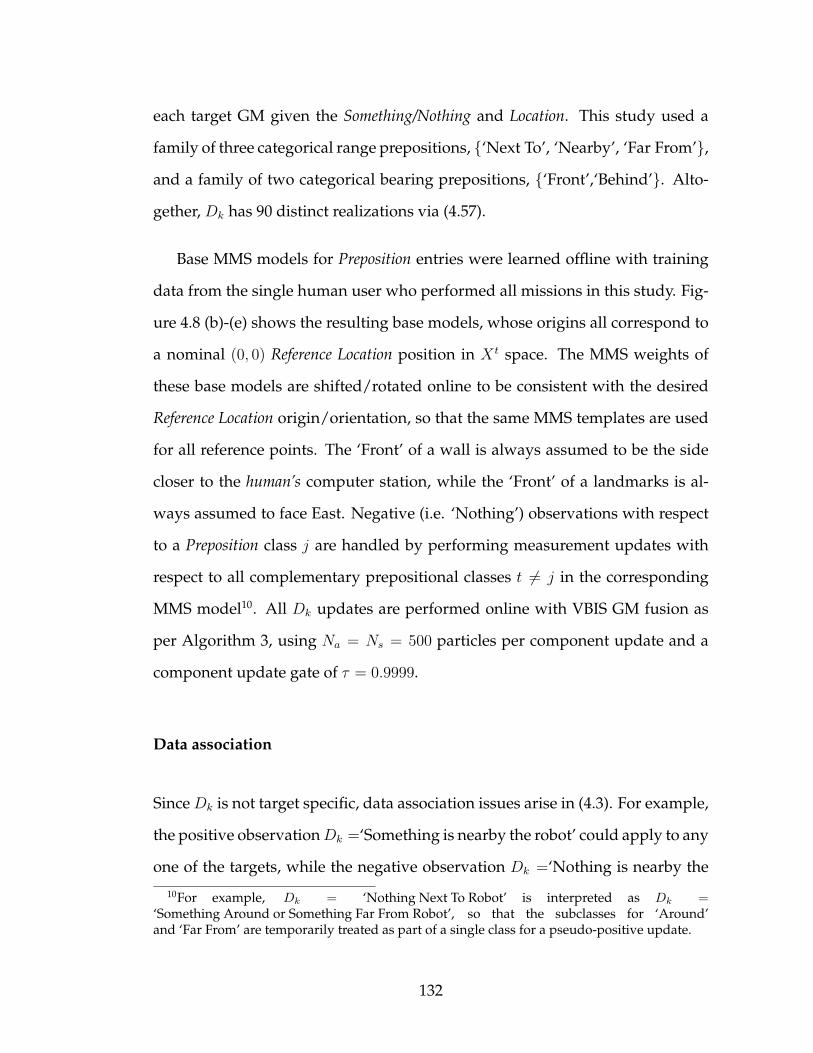
each target GM given the Something/Nothing and Location. This study used a
family of three categorical range prepositions, {‘Next To’, ‘Nearby’, ‘Far From’},
and a family of two categorical bearing prepositions, {‘Front’,‘Behind’}. Alto-
gether, Dk
has 90 distinct realizations via (4.57).
Base MMS models for Preposition entries were learned offline with training
data from the single human user who performed all missions in this study. Fig-
ure 4.8 (b)-(e) shows the resulting base models, whose origins all correspond to
a nominal (0, 0) Reference Location position in X t space. The MMS weights of
these base models are shifted/rotated online to be consistent with the desired
Reference Location origin/orientation, so that the same MMS templates are used
for all reference points. The ‘Front’ of a wall is always assumed to be the side
closer to the human’s computer station, while the ‘Front’ of a landmarks is al-
ways assumed to face East. Negative (i.e. ‘Nothing’) observations with respect
to a Preposition class j are handled by performing measurement updates with
respect to all complementary prepositional classes t 6= j in the corresponding
MMS model10. All Dk
updates are performed online with VBIS GM fusion as
per Algorithm 3, using Na
= Ns
= 500 particles per component update and a
component update gate of ⌧ = 0.9999.
Data association
Since Dk
is not target specific, data association issues arise in (4.3). For example,
the positive observation Dk
=‘Something is nearby the robot’ could apply to any
one of the targets, while the negative observation Dk
=‘Nothing is nearby the10For example, D
k
= ‘Nothing Next To Robot’ is interpreted as D
k
=‘Something Around or Something Far From Robot’, so that the subclasses for ‘Around’and ‘Far From’ are temporarily treated as part of a single class for a pseudo-positive update.
132

(a) (b) (c) (d) (e)
(f) (g) (h) (i) (j)
Figure 4.8: (a) Example GM target location prior, (b-d) base MMS modelsfor human descriptors, (e) base MMS model for camera detec-tion likelihood, (f-i) posterior GMs from VBIS after fusion ofmodels in (a-d) with GM prior in (a), (j) posterior GM fromLWIS after fusion of ‘No Detection’ report with GM prior in(a).
robot’ applies equally to all targets. This ambiguity is handled probabilistically
through the GM-based generalization of probabilistic data association (PDA)
[73]. First, (4.3) is computed as under the hypothesis that Dk
associates to target
t to give p⇤(Xt|⇣1:k, D1:k). This pdf is then combined with the pre-fusion prior
p(X t|⇣1:k, D1:k�1) (which represents the hypothesis that Dk
does not associate to
t) to give another GM that marginalizes the association hypothesis,
p(X t|⇣1:k, D1:k) = �(⌘) · p⇤(X t|⇣1:k, D1:k) + ⌘ · [1� �(⌘)] · p(X t|⇣1:k, D1:k�1)
(4.58)
where ⌘ = 1 if Dk
represents positive information (⌘ = 0 otherwise), and �(⌘)
is the probability of the hypothesis that Dk
associates to target t. Here, �(0) = 1
and �(1) = 1|Tk|
, where |Tk
| is the number of undetected targets at time k 11. The
probability of an erroneous/false human observation is assumed to be zero for11since all target t priors are initially the same, this is equivalent to setting �(⌘) = P (D
k
= j; t),i.e. the marginal likelihood of D
k
= j under target t, as in conventional PDA hypothesis mixing.This is also equal to a conservative maximum entropy estimate of association probability
133

convenience, although non-zero error/false alarm probabilities can be incorpo-
rated into (4.58) in a Bayesian manner while still maintaining a GM representa-
tion [73, 96].
Mixture condensation
Following each ⇣k
and Dk
update, each p(X t|⇣1:k, D1:k) is condensed to M = 15
mixands via Salmond’s merging algorithm [119], which sequentially combines
mixands to preserve the overall GM mean and covariance ( see [119] for de-
tails)12. Note that merging requires O(M2o
) time for Mo
initial mixands, which
limits online processing speed when each GM has hundreds of components 13.
Hence, brutal truncation is performed first to retain only the 100 most highly
weighted components of each p(X t|⇣1:k, D1:k) for merging.
4.5.3 Target priors and fusion scenarios
To assess the relative effects of ⇣k
and Dk
and different initial target priors on
the fusion process, four sets of search missions were conducted under three
types of sensing modalities (‘Robot Only’,‘Human Only’, and ‘Human with
Robot’) and two types of initial target search GM priors (‘(Pseudo)-Uniform’,
‘Bad/Inconsistent’). Table 4.3 shows the resulting experimental matrix of 24
total search missions, in which the human always confirmed target detec-
tions/false alarms and the robot navigated autonomously via the greedy search
algorithm, regardless of sensing modality. Four target search missions were12similar results were obtained with Runnalls’ KLD-based merging algorithm [117], which
costlier to implement13this can arise from certain negative D
k
updates, such as ‘Nothing is nearby the robot’
134

Table 4.3: Experimental Search Mission Matrix for Human-Robot Team
Prior type/Sensing Modality Robot Only Human Only Human With Robot
Pseudo-uniform GM Prior 4 missions without eq.(4.2) updates 4 missions without eq.(4.3) updates 4 missions w/ eq.(4.2) and (4.3) updates
Bad/Inconsistent GM Prior 4 missions without eq.(4.2) updates 4 missions without eq.(4.3) updates 4 missions w/ eq.(4.2) and (4.3) updates
used to study each cell of Table 4.3; each mission was characterized by a dif-
ferent set of true target locations and the same four missions are used to study
all cells of Table 4.3. The true target location maps for each mission are shown
in Figure 4.9(a)-(d), where missions 1 and 4 used the same target location map
14. As shown in Fig. 4.9(d), the pseudo-uniform GM prior for each mission
used Mt
= 8 spherical mixands with ⌃u
i
= I to reflect the initial belief that tar-
gets can be located anywhere on the map with (almost) equal probability. The
bad GM priors shown in Fig. 4.9(a)-(c) used Mt
= 5 spherical components that
were highly inconsistent with the true target locations in each mission, reflecting
worst-case search scenarios where a priori target information is badly flawed.
Missions under uniform prior and ‘Human With Robot’ sensing modality
were conducted first, followed by the corresponding ‘Human Only’ and ‘Robot
Only’ missions; the missions were then repeated in the same order using bad
priors. To simulate realistic target discovery in all cases with the same human
operator, the human did not send positive (i.e. ‘Something is...’) information
about targets unless they were either directly visible to the human or glimpsed
in the robot’s camera during the mission15. All experimental missions reported
here were immediately stopped if the robot could not find all targets in under 15
minutes (900 secs). This challenging time constraint was chosen after extensive14the cones were initially labeled with white paper tags in mission 1, which inadvertently
decreased the probability of visual detection by the robot; the cones were relabeled in missions2 through 4 to improve visibility
15e.g. in mission 1 runs, the human could not establish a direct line of sight to target 3 andtherefore did not furnish relevant information about that target until after seeing it via camera
135

(a) (b)
(c) (d)
Figure 4.9: True target locations and initial GM priors used in each mis-sion, showing ‘bad’ (a-c) and ‘uniform’ (d) search priors. Theuniform GM prior in (d) is the same in all four search missionsand the bad priors for missions 1 and 4 are the same.
testing with the greedy search strategy, which showed that 15-25 minutes are
generally required to find all five targets in missions 1-4 using ‘Robot Only’
sensing and uniform prior conditions.
4.5.4 Results: overall search performance
The overall search performance of the human-robot team under different sens-
ing and a priori information scenarios can be gauged via the search comple-
tion time and number of targets detected in each search mission. Fig. 4.10
shows the results for these two metrics over all 24 search missions. ‘Human
With Robot’ sensing clearly offers the best overall search performance, since all
136

0 200 400 600 800
1
2
3
4
Search Times for Each Mission with Uniform Prior
Trial time (sec)
Mis
sion
Num
ber
Robot OnlyHuman OnlyHuman + Robot
0 200 400 600 800
1
2
3
4
Search Times on Each Mission with Bad Prior
Trial time (sec)
Mis
sion
Num
ber
Robot OnlyHuman OnlyHuman + Robot
(a) (b)
1 2 3 40
1
2
3
4
5Number of Targets Found on Each Mission with Uniform Prior
Mission Number
Num
ber o
f Tar
gets
Fou
nd
Robot OnlyHuman OnlyHuman + Robot
1 2 3 40
1
2
3
4
5Number of Targets Found on Each Mission with Bad Prior
Mission Number
Num
ber o
f Tar
gets
Fou
nd
Robot OnlyHuman OnlyHuman + Robot
(c) (d)
Figure 4.10: Overall search mission performance under different priortypes and sensing modalities: (a)-(b) search mission times(secs) under uniform and bad priors, respectively; (c)-(d)number of targets found per mission under uniform and badpriors, respectively.
5 targets were always found in each mission within 8.5-13 minutes. While more
targets were found under ‘Human Only’ sensing than under ‘Robot Only’ sens-
ing (which has the worst overall performance), the mission completion times
for these two sensing modalities were about the same. The number of target
detections for each of these two sensing modalities drops slightly when mov-
ing from uniform to bad GM search priors; in constrast, the prior type did not
significantly affect performance with ‘Human With Robot’ sensing.
The ‘Robot Only’ performance results underscore the nontrivial nature of the
137

search problem and the inadequacy of the robot’s greedy search strategy when
only ⇣k
measurement updates are available. When Dk
is available, the robot be-
comes much more proficient at detecting targets via the greedy search (though
performance is not necessarily ‘optimal’ in any sense). The improvement from
human input can be explained by comparing the typical level of informative-
ness of p(X t|D1:k, ⇣1:k) over time under the various fusion and prior conditions.
Fig. 4.11 shows time traces from all six mission 4 runs of the posterior proba-
bility of finding target t inside a 1 m square region R(X t
true) centered at X t
true (i.e.
the belief that t is located close to its true unknown location). This probability is
computed offline at each time step k as
P (R(X t
true)|D1:k, ⇣1:k) =
Z
R(Xttrue)
p(X t|⇣1:kD1:k)dXt
. (4.59)
Note that (4.59) approaches 1 as p(X t|⇣1:kD1:k) becomes more highly concen-
trated inside R(X t
true).
To illustrate the typical frequency of voluntary human-to-robot communi-
cation and its influence on each P (R(X t
true)|D1:k, ⇣1:k), Fig. 4.11 also shows all
instances when human observations Dk
were sent and fused. Despite being
highly rate-limited and imprecise, human observations Dk
were generally in-
formative enough to quickly increase P (R(X t
true)|D1:k, ⇣1:k) so that targets could
be easily detected by the robot’s greedy search in the ‘Human Only’ and ‘Hu-
man With Robot’ missions. In contrast, P (R(X t
true)|D1:k, ⇣1:k) increases at a much
slower rate using only ⇣k
updates in the ‘Robot Only’ missions. This has partic-
ularly severe consequences in the ‘Robot Only’ scenarios with bad priors, where
the a priori probability of finding the targets at their true locations is extremely
small (typically on the order of 1⇥ 10
�35).
138

0 100 200 300 400 500 600 700 800 9000
0.1
0.2
0.3
0.4
0.5
0.6
0.7
0.8
0.9
1
Time Step, k
Targ
et R
egio
n P
roba
bilit
y
RobotOnly Uniform trial 4
Target 1 Prob.Target 2 Prob.Target 3 Prob.Target 4 Prob.Target 5 Prob.Target Detection
0 100 200 300 400 500 600 700 800 9000
0.1
0.2
0.3
0.4
0.5
0.6
0.7
0.8
0.9
1
Time Step, k
Targ
et R
egio
n P
roba
bilit
y
HumanOnly Uniform trial 4
Target 1 Prob.Target 2 Prob.Target 3 Prob.Target 4 Prob.Target 5 Prob.Human MessageTarget Detection
0 100 200 300 400 500 600 700 800 9000
0.1
0.2
0.3
0.4
0.5
0.6
0.7
0.8
0.9
1
Time Step, k
Targ
et R
egio
n P
roba
bilit
y
HumanWRobot Uniform trial 4
Target 1 Prob.Target 2 Prob.Target 3 Prob.Target 4 Prob.Target 5 Prob.Human MessageTarget Detection
(a) (b) (c)
0 100 200 300 400 500 600 700 800 9000
0.1
0.2
0.3
0.4
0.5
0.6
0.7
0.8
0.9
1
Time Step, k
Targ
et R
egio
n P
roba
bilit
y
RobotOnly BadPrior trial 4
Target 1 Prob.Target 2 Prob.Target 3 Prob.Target 4 Prob.Target 5 Prob.Target Detection
0 100 200 300 400 500 600 700 800 9000
0.1
0.2
0.3
0.4
0.5
0.6
0.7
0.8
0.9
1
Time Step, k
Targ
et R
egio
n P
roba
bilit
y
HumanOnly BadPrior trial 4
Target 1 Prob.Target 2 Prob.Target 3 Prob.Target 4 Prob.Target 5 Prob.Human MessageTarget Detection
0 100 200 300 400 500 600 700 800 9000
0.1
0.2
0.3
0.4
0.5
0.6
0.7
0.8
0.9
1
Time Step, k
Targ
et R
egio
n P
roba
bilit
y
HumanWRobot BadPrior trial 4
Target 1 Prob.Target 2 Prob.Target 3 Prob.Target 4 Prob.Target 5 Prob.Human MessageTarget Detection
(d) (e) (f)
Figure 4.11: P (R(X t
true)|D1:k, ⇣1:k) vs. time step k for various fusion scenar-ios in the mission 4 setup: (a)-(c) Uniform prior with cam-era only, human only, and human with robot updates, respec-tively, (d)-(f) Bad prior with camera only, human only, andhuman with robot updates, respectively. Dashed vertical linesdenote target detection events; black markers on the time axisdenote human observation instances.
4.5.5 Results: Diversity of Soft Human Sensor Inputs
Fig. 4.14 illustrates the observed counts of Preposition and Reference Location
codebook counts in each ‘Human Only’ and ‘Human With Robot’ mission,
where the number of positive and negative messages are also shown at the top
of each frequency matrix. The volume of messages is significantly larger with a
bad prior than with a uniform prior, as the human had to work harder to ‘con-
vince’ the robot to shift more probability mass towards actual target locations in
bad prior conditions. There were also many more positive messages (1376) than
139

negative messages (296) over all search scenarios, due to the fact that the con-
tribution of the association hypothesis pdf p⇤(Xt|⇣1:k, D1:k) following positive
‘Something is...’ messages were downweighted via the PDA correction in eq.
(4.58). Hence, even with benign priors, the human had to ‘convince’ robot that
‘something’ was in fact somewhere by repeatedly sending the same positive in-
formation message multiple times. Since negative information (‘Nothing is...’)
messages were more potent in reshaping the target pdfs with fewer messages,
since they were not downweighted by PDA.
4.5.6 Complementary Team Behavior
As pointed out in [21], a simple greedy search strategy generally leads to ineffi-
cient ‘back and forth’ search paths over the map as a direct consequence of the
scattering effect from ⇣k
updates (cf. Fig. 4.8 (l)). As such, in ‘Robot Only’ sce-
narios, the robot frequently jumped from one part of the search map to another
without searching thoroughly around its goal points, leading to very slow in-
formation gain. Additional difficulties in the mission 1 ‘Robot Only’ cases arose
from the fact that all targets were labeled with white tags and were therefore
less likely to be detected, despite being within the nominal 1 m visual detection
range 16. Since eq. (4.56) diminished around missed X t
true following missed de-
tections, the robot could not remedy missed target detections until after greedily
searching the rest of the map. As Fig. 4.12 illustrates, in ‘Human With Robot’
scenarios, the human operator could quickly correct missed detections by send-
ing relevant soft information that forced the robot to greedily re-examine areas
around actual target locations (this was particularly useful in mission 1).16e.g. compare the Uniform prior results of mission 1 to those of mission 4, which used the
same target locations as in mission 1
140

(a) (b) (c)
(d) (e) (f)
Figure 4.12: ‘Human With Robot’ sensing sequence showing soft humancorrection of missed target detections with ⇣
k
updates: (a)robot (pink) explores GM peak near target 1, but cannot detecttarget 1 just at the edge of its field of view (green triangle); (b)robot turns to go explore new pdf peak that appeared behindtarget 2 via scattering effect; (c) human message ‘Something isNearby Landmark 1’ boosts pdf value near target 1; (d) robotgoes back to explore around target 1, but misses it again; (e)human message ‘Something is Behind Robot’ boosts pdf neartarget 1 again; (f) robot successfully finds target 1. Total se-quence time is just over 1 minute.
Although ‘Human Only’ sensing leads to more target detections than ‘Robot
Only’ sensing, some targets remain undetected in certain missions and comple-
tion times are not improved consistently (especially in bad prior missions). This
can be largely attributed to the coarse nature of the soft Dk
codebook, which
meant that eq. (4.56) could not be precisely updated to allow the robot to ‘nudge
closer’ toward the target if it was just outside the robot’s visual detection range.
As Fig. 4.13 illustrates, the human spent considerable time in ‘Human Only’
141

missions compensating for this issue by sending many extra messages to ‘con-
vince’ the robot into obtaining a better viewing position for certain targets. The
resulting high volume of Dk
messages (especially in the bad prior missions) is
also evident in Fig. 4.14 (a) and Fig. 4.11 (b) and (e). These scenarios not only
account for the lack of significant mission time improvements and the fact that
some targets were not found, but also caused the human to become frustrated.
However, in ‘Human With Robot’ cases, scattering via ⇣k
= ‘No Detection’ ob-
servations helped shift eq. (4.56) closer to any targets just outside of detection
range, thereby automatically refining the target posterior GMs following Dk
up-
dates. This also led to smoother interaction between the human and robot, as
indicated by the significantly improved mission times and lower message vol-
ume/frequency compared with ‘Human Only’ missions.
4.5.7 Accuracy of GM data fusion approximations
To assess the accuracy of online fusion of ⇣k
data via LWIS and of Dk
data via
VBIS in each search mission, the KL divergence (KLD) of each GM posterior
p(X t|⇣1:k, D1:k) obtained at every time step k was computed offline for all search
missions with respect to recursive grid-based ‘ground truth’ fusion posteriors,
which used 0.1 m ⇥0.1 m cell resolution. To further assess the contribution of
VBIS in the ‘Human Only’ and ‘Human With Robot’ missions, KLDs were also
computed offline for a separate set of GM posteriors obtained by fusing both ⇣1:k
and D1:k via LWIS GM mixture fusion with 1000 samples per component update
(to match the total number of sampling operations used for VBIS Dk
updates).
The KLDs for both the online LWIS-VBIS and offline LWIS-only GM approxima-
tions were evaluated over 10 independent Monte Carlo runs to account for ran-
142
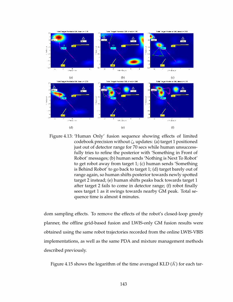
(a) (b) (c)
(d) (e) (f)
Figure 4.13: ‘Human Only’ fusion sequence showing effects of limitedcodebook precision without ⇣
k
updates: (a) target 1 positionedjust out of detector range for 70 secs while human unsuccess-fully tries to refine the posterior with ‘Something in Front ofRobot’ messages; (b) human sends ‘Nothing is Next To Robot’to get robot away from target 1; (c) human sends ‘Somethingis Behind Robot’ to go back to target 1; (d) target barely out ofrange again, so human shifts posterior towards newly spottedtarget 2 instead; (e) human shifts peaks back towards target 1after target 2 fails to come in detector range; (f) robot finallysees target 1 as it swings towards nearby GM peak. Total se-quence time is almost 4 minutes.
dom sampling effects. To remove the effects of the robot’s closed-loop greedy
planner, the offline grid-based fusion and LWIS-only GM fusion results were
obtained using the same robot trajectories recorded from the online LWIS-VBIS
implementations, as well as the same PDA and mixture management methods
described previously.
Figure 4.15 shows the logarithm of the time averaged KLD ( ¯K) for each tar-
143

get GM posterior in the ‘Robot Only’ uniform and bad prior missions, where
only LWIS is used to fuse ⇣k
. These results show that 15 component GMs pro-
vide good approximations to the exact grid-based target location posteriors over
the course of a full 15 minute search mission. Although not apparent from
these plots, the KLDs at each time step tend to drift up very slowly over as
information is gradually lost with respect to the true posterior. Such baseline
losses are expected, since 15 smooth and symmetric Gaussian components can
only approximate the highly asymmetric and multimodal exact target posteriors
with limited precision (especially as these change quite rapidly over time). Fur-
ther baseline losses are incurred over time through mixture reduction via brutal
truncation and Salmond’s algorithm, which does not preserve GM information
above second order moments. Nevertheless, it is clear that the expected baseline
information losses incurred by fusing ⇣1:k through LWIS are small enough over
the course of a full 15 minute search mission to justify using GM approximations
for the probabilistic search.
Figure 4.16 (a)-(b) show ¯Ks for LWIS-VBIS and LWIS-only fusion using uni-
form priors in the ‘Human With Robot’ and ‘Human Only’ cases. These results
show that, when prior information and human observations are generally con-
sistent with each other, LWIS with 1000 samples per component update and
VBIS with 500 samples per component update offer comparably good fusion
accuracy. Note that, in missions 2 and 3 of the ‘Human Only’ cases, the pos-
terior for some targets grew significantly more complex at certain time steps
following certain prolonged sequences of human observations. As a result, the
tails and several small components of the true posterior pdfs could not be well-
modeled by 15 component GMs following either VBIS and LWIS fusion after
certain points in time, leading to higher ¯K values for some targets. This diver-
144

gence phenomenon nevers occurs for ‘Human With Robot’ fusion with either
the LWIS-VBIS or LWIS-only update methods, as the use of benign uniform
priors and the fusion of ⇣1:k helped reduced the number of human messages
needed to modify the target pdfs (thus limiting the complexity of the posteri-
ors).
Figure 4.16 (c)-(d) show the ¯Ks for LWIS-VBIS and LWIS-only fusion using
bad priors in the ‘Human With Robot’ and ‘Human Only’ cases. These plots
also denote several cases where LWIS-VBIS fusion shows a statistically signifi-
cant ¯K improvement over LWIS-only fusion (using a Kruskall-Wallis test with
p = 0.01). These results confirm the notion that VBIS is more reliable than LWIS
for fusing Dk
when the prior is possibly inconsistent with the true target state.
This is especially apparent from the smaller ¯Ks in missions 1 and 4, which show
that VBIS provides more accurate approximations for the ‘suprising’ human ob-
servations on almost every target. Due to the limited number of available GM
components, both VBIS and LWIS still obtain some high ¯Ks under bad priors
and/or ‘Human Only’ fusion conditions, which typically had more complex
posteriors due to increased Dk
messaging. It is important to note that the LWIS
Dk
fusion results in Fig. 4.16 greatly benefit from the JPDA-based positive mes-
sage updates in eq. (4.58), since this always incorporates a substantial portion
of the prior into the GM posterior (i.e. the prior weight 1 � �(⌘) ranges from
0.5 to 0.8). Although not shown here due to limited space, the use of either
target-specific updates (obtained by hand-labeling) to eliminate data associa-
tion ambiguity gives significantly worse KLD losses per Dk
update for LWIS in
all bad prior cases, whereas VBIS accuracy remains unaffected.
145

4.5.8 Computational speed and storage
Despite its improved reliability, VBIS is slightly more expensive to implement
than LWIS. In particular, VBIS requires approximately 7 ms on average per GM
component update in these experiments using managed C# code, while LWIS
requires approximately 2 ms on average17. The longer VBIS times stem from the
fact that Algorithm 1 can converge slowly if it is initialized far from the final
solution. However, even in such cases, VBIS computation times can be signif-
icantly reduced through several code optimization strategies not implemented
here, such as: parallelization of Algorithm 3; clustering of VBEM initializations
across similar GM components within and across target GM pdfs; and imple-
mentation of unmanaged pointer arithmetic code. Such optimizations were un-
necessary for the present application, as VBIS did not lead to significant delays
for real-time operation with the human operator.
The online-computed GM approximations used to represent the target pos-
terior pdfs require considerably less memory and communication bandwidth
than the offline-computed ground truth discrete grids. For a single time step, a
15 component GM approximation for a single target posterior requires 840 bytes
using double precision, while the ground-truth grid requires approximately 52
times as much memory at 44,064 bytes. Hence, for a full 900 sec search mission,
a full time history of the GM filtering posterior recorded at 2 Hz requires 1.51
MB, compared with 79.32 MB for a grid-based filtering history. Although not
demonstrated here, the storage discrepency between the two representations
becomes even larger if Xk
includes additional states (e.g. vertical displacement,
velocities). Such storage costs are especially relevant in data fusion applications17these times did not increase significantly when the component gating threshold ⌧ is in-
creased to � 1 to update all GM components
146

in which pdfs over multiple time steps must be stored and/or communicated,
e.g. for decentralized data fusion in distributed sensor networks [95, 71].
4.6 Discussion and Conclusions
4.6.1 How should human sensors be used?
Soft categorical ‘human sensor’ observations can be exploited in many differ-
ent dynamic data fusion domains and are particularly convenient in situations
where humans agents must communicate information quickly but do not have
enough time to precisely estimate particular states of interest (e.g. the precise
range and bearing to a target in meters and degrees, respectively). While the ex-
periments here show that soft human observations alone can lead to a substantial
reduction in uncertainty through proper Bayesian fusion, it is clear that over-
reliance on soft human information can also have undesirable consequences in
practical settings. For instance, it is possible to reach a stage in the dynamic data
fusion process where soft human data reports alone no longer add useful new
information to the prior pdf without further information from other sensors, as
shown in Fig. 4.13 (a). As such, it is important in any application to account for
the facts that: (i) human inputs are rate-limited by cognitive processing and sig-
nal communication delays; (ii) soft categorical observations can only coarsely
shape the state pdf up to the effective resolution of the sensor model (which de-
pends on both the model’s base parameters and the number of ways in which
the model reference frame can be shifted/rotated in Xk
space); and (iii) fusion
of soft human data can sometimes increase the complexity of the Xk
pdf (e.g. if
147

negative information introduces additional modes via scattering).
Therefore, it is important both to specify/learn likelihood models with ap-
propriate granularity levels and contextual reference points with respect to Xk
and to ensure that other data sources are available for more persistent and pre-
cise refinement of the Xk
pdf. Note that if more refined continuous human
observations Ck
are available for a particular application, then these can also be
incorporated into the Bayesian data fusion loop of Fig.4.1 as additional data to
update p(Xk
|D1:k, ⇣1:k). This extension is especially straightforward if each Ck
is described by a linear-Gaussian or Gaussian mixture likelihood model as in
ref. [76], since this leads to closed-form EKF-like measurement updates for each
mixand of the approximate hybrid GM posterior derived in eq. (4.53). Further-
more, estimates of human sensor error/false alarm probabilities and likelihood
model uncertainties can be incorporated into the proposed Bayesian data fusion
process in the same manner as for conventional robot sensors [96].
4.6.2 Conclusion
This paper derived a computationally efficient and accurate approximation to
the recursive hybrid Bayesian inference problem involved in the dynamic fu-
sion of soft categorical human observations with conventional hard robot sensor
data. The proposed VBIS fusion method combines the strengths of fast stand-
alone variational Bayes and Monte Carlo importance sampling inference ap-
proximations to obtain consistent Gaussian posteriors in the baseline case of
Gaussian state priors with softmax likelihood functions. VBIS was then ex-
tended to derive GM posterior approximations for GM priors with MMS like-
148

lihood models in order to handle more general recursive hybrid data fusion
problems. Experimental multitarget search results for a real human-robot team
showed that soft categorical observations from ‘human sensors’, although sub-
ject to limited precision and potential data association ambiguities, can still be
highly useful and informative for recursive Bayesian estimation problems fea-
turing a high degree of uncertainty or inconsistency. The results also provide
valuable practical insight into the reliability of the proposed VBIS GM approxi-
mations under a variety of fusion conditions, vis-a-vis LWIS GM and grid-based
ground truth approximations.
149

HumanOnly Uniform Trial 1,(P/N: 162/12)
Preposition
Ref
. Loc
atio
n
NextTo Around FarFrom Front Behind
l1
l2
w1
w2
w3
w4
w5
w6
r
HumanOnly Uniform Trial 2,(P/N: 71/27)
Preposition
Ref
. Loc
atio
n
NextTo Around FarFrom Front Behind
l1
l2
w1
w2
w3
w4
w5
w6
r
HumanOnly Uniform Trial 3,(P/N: 147/30)
Preposition
Ref
. Loc
atio
n
NextTo Around FarFrom Front Behind
l1
l2
w1
w2
w3
w4
w5
w6
r
HumanOnly Uniform Trial 4,(P/N: 35/18)
Preposition
Ref
. Loc
atio
n
NextTo Around FarFrom Front Behind
l1
l2
w1
w2
w3
w4
w5
w6
r
HumanOnly BadPrior Trial 1,(P/N: 165/23)
Preposition
Ref
. Loc
atio
n
NextTo Around FarFrom Front Behind
l1
l2
w1
w2
w3
w4
w5
w6
r
HumanOnly BadPrior Trial 2,(P/N: 79/27)
Preposition
Ref
. Loc
atio
n
NextTo Around FarFrom Front Behind
l1
l2
w1
w2
w3
w4
w5
w6
r
HumanOnly BadPrior Trial 3,(P/N: 208/20)
Preposition
Ref
. Loc
atio
nNextTo Around FarFrom Front Behind
l1
l2
w1
w2
w3
w4
w5
w6
r
HumanOnly BadPrior Trial 4,(P/N: 96/33)
Preposition
Ref
. Loc
atio
n
NextTo Around FarFrom Front Behind
l1
l2
w1
w2
w3
w4
w5
w6
r
0
2
4
6
8
10
12
14
16
18
20
(a)HumanWRobot Uniform Trial 1,
(P/N: 39/7)
Preposition
Ref
. Loc
atio
n
NextTo Around FarFrom Front Behind
l1
l2
w1
w2
w3
w4
w5
w6
r
HumanWRobot Uniform Trial 2,(P/N: 22/23)
Preposition
Ref
. Loc
atio
n
NextTo Around FarFrom Front Behind
l1
l2
w1
w2
w3
w4
w5
w6
r
HumanWRobot Uniform Trial 3,(P/N: 17/20)
Preposition
Ref
. Loc
atio
n
NextTo Around FarFrom Front Behind
l1
l2
w1
w2
w3
w4
w5
w6
r
HumanWRobot Uniform Trial 4,(P/N: 40/10)
Preposition
Ref
. Loc
atio
n
NextTo Around FarFrom Front Behind
l1
l2
w1
w2
w3
w4
w5
w6
r
HumanWRobot BadPrior Trial 1,(P/N: 125/2)
Preposition
Ref
. Loc
atio
n
NextTo Around FarFrom Front Behind
l1
l2
w1
w2
w3
w4
w5
w6
r
HumanWRobot BadPrior Trial 2,(P/N: 50/25)
Preposition
Ref
. Loc
atio
n
NextTo Around FarFrom Front Behind
l1
l2
w1
w2
w3
w4
w5
w6
r
HumanWRobot BadPrior Trial 3,(P/N: 76/8)
Preposition
Ref
. Loc
atio
n
NextTo Around FarFrom Front Behind
l1
l2
w1
w2
w3
w4
w5
w6
r
HumanWRobot BadPrior Trial 4,(P/N: 44/11)
Preposition
Ref
. Loc
atio
n
NextTo Around FarFrom Front Behind
l1
l2
w1
w2
w3
w4
w5
w6
r0
5
10
15
20
(b)
Figure 4.14: Frequencies of Preposition and Reference Location entries in human mes-sages over all missions for Uniform and Bad Prior conditions: (a) Humanonly measurement update scenario results, (b) Human+Robot measure-ment update scenario results. Counts are saturated above 20 messagesto create a uniformly scaled display across all missions. Reference pointsalong y-axis are l# = landmark #, w# = wall #, r = robot. P/N denotesnumber of positive/negative messages.
150
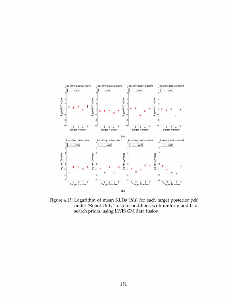
1 2 3 4 5!3
!2
!1
0
1
2
3
4RobotOnly BadPrior trial#1
log
mK
LD v
alue
Target Number
LWIS
1 2 3 4 5!3
!2
!1
0
1
2
3
4RobotOnly BadPrior trial#2
log
mK
LD v
alue
Target Number
LWIS
1 2 3 4 5!3
!2
!1
0
1
2
3
4RobotOnly BadPrior trial#3
log
mK
LD v
alue
Target Number
LWIS
1 2 3 4 5!3
!2
!1
0
1
2
3
4RobotOnly BadPrior trial#4
log
mK
LD v
alue
Target Number
LWIS
(a)
1 2 3 4 5!3
!2
!1
0
1
2
3
4RobotOnly Uniform trial#1
log
mK
LD v
alue
Target Number
LWIS
1 2 3 4 5!3
!2
!1
0
1
2
3
4RobotOnly Uniform trial#2
log
mK
LD v
alue
Target Number
LWIS
1 2 3 4 5!3
!2
!1
0
1
2
3
4RobotOnly Uniform trial#3
log
mK
LD v
alue
Target Number
LWIS
1 2 3 4 5!3
!2
!1
0
1
2
3
4RobotOnly Uniform trial#4
log
mK
LD v
alue
Target Number
LWIS
(b)
Figure 4.15: Logarithm of mean KLDs ( ¯Ks) for each target posterior pdfunder ‘Robot Only’ fusion conditions with uniform and badsearch priors, using LWIS GM data fusion.
151

1 2 3 4 5!3
!2
!1
0
1
2
3
4
5HumanOnly Uniform trial#1
log
mK
LD v
alue
Target Number
LWISVBIS
1 2 3 4 5!3
!2
!1
0
1
2
3
4
5HumanOnly Uniform trial#2
log
mK
LD v
alue
Target Number
LWISVBIS
1 2 3 4 5!3
!2
!1
0
1
2
3
4
5HumanOnly Uniform trial#3
log
mK
LD v
alue
Target Number
LWISVBIS
1 2 3 4 5!3
!2
!1
0
1
2
3
4
5HumanOnly Uniform trial#4
log
mK
LD v
alue
Target Number
LWISVBIS
(a)
1 2 3 4 5!3
!2
!1
0
1
2
3
4
5HumanWRobot Uniform trial#1
log
mK
LD v
alue
Target Number
LWIS!onlyLWIS!VBIS
1 2 3 4 5!3
!2
!1
0
1
2
3
4
5HumanWRobot Uniform trial#2
log
mK
LD v
alue
Target Number
LWIS!onlyLWIS!VBIS
1 2 3 4 5!3
!2
!1
0
1
2
3
4
5HumanWRobot Uniform trial#3
log
mK
LD v
alue
Target Number
LWIS!onlyLWIS!VBIS
1 2 3 4 5!3
!2
!1
0
1
2
3
4
5HumanWRobot Uniform trial#4
log
mK
LD v
alue
Target Number
LWIS!onlyLWIS!VBIS
(b)
1 2 3 4 5!3
!2
!1
0
1
2
3
4
5HumanOnly BadPrior trial#1
log
mK
LD v
alue
Target Number
LWISVBIS
1 2 3 4 5!3
!2
!1
0
1
2
3
4
5HumanOnly BadPrior trial#2
log
mK
LD v
alue
Target Number
LWISVBIS
1 2 3 4 5!3
!2
!1
0
1
2
3
4
5HumanOnly BadPrior trial#3
log
mK
LD v
alue
Target Number
LWISVBIS
1 2 3 4 5!3
!2
!1
0
1
2
3
4
5HumanOnly BadPrior trial#4
log
mK
LD v
alue
Target Number
LWISVBIS
(c)
1 2 3 4 5!3
!2
!1
0
1
2
3
4
5HumanWRobot BadPrior trial#1
log
mK
LD v
alue
Target Number
LWIS!onlyLWIS!VBIS
1 2 3 4 5!3
!2
!1
0
1
2
3
4
5HumanWRobot BadPrior trial#2
log
mK
LD v
alue
Target Number
LWIS!onlyLWIS!VBIS
1 2 3 4 5!3
!2
!1
0
1
2
3
4
5HumanWRobot BadPrior trial#3
log
mK
LD v
alue
Target Number
LWIS!onlyLWIS!VBIS
1 2 3 4 5!3
!2
!1
0
1
2
3
4
5HumanWRobot BadPrior trial#4
log
mK
LD v
alue
Target Number
LWIS!onlyLWIS!VBIS
(d)
Figure 4.16: Logarithm of mean KLDs ( ¯Ks) for each target posterior pdfunder ‘Human Only’ and ‘Human With Robot’ fusion con-ditions with uniform and bad search priors, using VBIS andLWIS GM data fusion. Stars on bottom axes denote instanceswhere VBIS for human data fusion achieves statistically sig-nificant lower ¯K than LWIS.
152

CHAPTER 5
CONCLUSIONS
5.1 Summary of contributions
5.1.1 Chapter 1
This chapter discussed the important roles humans play in multi-robot systems
and highlighted the cognitive limitations faced by humans when dealing with
autonomous machines. This motivated the question of how to best combine hu-
man and robot capabilities for practical applications. Three important issues
stemming from this key question were then outlined to motivate the devel-
opment of models that could be used to: (1) predict human supervisory con-
trol performance, (2) predict human strategic supervisory decision-making out-
comes, and (3) extract useful information from human observations. The use of
descriptive probabilistic models in this thesis was justified, and the background
and main contributions for each chapter was discussed.
5.1.2 Chapter 2
This chapter examined the prediction of human supervisory performance in
large-scale networked robotic teams. It was shown that metrics of human super-
visory performance in large-scale networked robotic teams could be probabilis-
tically predicted on the basis of individual factors and task/network-related fac-
tors. In particular, analysis of experimental human operator data from a multi-
153

UAV air defense simulation suggested that working memory capacity measures
could be used to significantly improve operator performance predictions under
different task load and communication quality conditions. This notion was sup-
ported by model validation results for three different probabilistic predictive
models based on linear regression, Bayesian networks, and Gaussian processes.
The practical advantages and limitations for each of these different probabilistic
predictive models was also discussed.
5.1.3 Chapter 3
This chapter developed new probabilistic learning techniques that are relevant
to the problem of discriminatively modeling human supervisors as strategic de-
cision makers in multi-robot teams. New variational Bayes (VB) learning ap-
proximations were derived for two latent softmax variable models: the multi-
modal softmax model and the mixture of expert discriminative models. The
proposed VB solutions overcome the limitations of previous Bayesian methods
for learning latent softmax variable model. Experiments with benchmark and
RoboFlag strategic human decision modeling data showed that the proposed
VB approximations are effective in practice. Comparisons to models learned
via the Bayes Information Criterion and to baseline nonlinear kernel classifiers
confirmed the soundness of the proposed VB approximations for Bayesian pa-
rameter estimation and model selection.
154

5.1.4 Chapter 4
This chapter developed new recursive Bayesian data fusion methods for com-
bining soft information obtained from imprecise human observations with
hard/soft information obtained from conventional robot sensors. It was shown
that soft human information could be modeled using discrete random variables
and softmax likelihood functions. The variational Bayesian importance sam-
pling (VBIS) algorithm was developed for the baseline case of Gaussian state
priors and softmax human likelihoods. VBIS was then extended to the more
general case of Gaussian mixture priors and multimodal softmax likelihoods.
An experimental multi-target search mission involving a real human-robot team
was used to validate the proposed fusion approach and provided insight into
the practical advantages and limitations of soft human-robot data fusion.
155

APPENDIX A
PROOF OF LOG-CONCAVITY FOR THE BASELINE
GAUSSIAN-SOFTMAX POSTERIOR
It is to be shown that the logarithm of (4.6) is a concave function of Xk
when
p(Xk
) = N (µ,⌃) and P (D = j|Xk
) is given by (4.7). Taking the log of (4.6) in
this case gives
log p(Xk
|D = j) = log p(Xk
) + logP (Dk
= j|Xk
)� logP (Dk
= j) = L1 + L2 � LC
LC
is the measurement log-likelihood, which is constant with respect to Xk
. L1
is the log of a Gaussian pdf, which is concave with respect to Xk
since its Hessian
is the negative semi-definite matrix �⌃ (where ⌃ is positive semi-definite by
definition). Since the sum of two concave functions of Xk
is also concave, the
concavity of L2 remains to be shown. Differentiating L2 with respect to Xk
twice
and simplifying gives the Hessian matrix,
H(Xk
) =
m
X
i=1
wi
P (D = i|Xk
)
m
X
l=1
wT
l
P (D = l|Xk
)� wT
i
!
= �m
X
i=1
wi
wT
i
· P (D = i|Xk
)
+
m
X
i=1
wi
· P (D = i|Xk
)
!
m
X
l=1
wl
· P (D = l|Xk
)
!
T
.
Next, define a random variable w that only takes values in {w1, ..., wm
} with
pdf �(w � wi
) · P (D = i|Xk
), where wi
2 Rd for i 2 {1, ...,m} and �(w � wi
) is
the Dirac delta function. This gives expectationsP
m
i=1 wi
· P (D = i|Xk
) = E [w]
andP
m
i=1 wi
wT
i
· P (D = i|Xk
) = E⇥
wwT
⇤
, so that H(Xk
) can be expressed as a
negative covariance matrix,
H(Xk
) = �(E ⇥wwT
⇤� E [w]E [w]T ). (A.1)
156

The negative semi-definiteness of H(Xk
) can thus be verified via Jensen’s in-
equality,
E [f(w)]� f(E [w]) � 0, (A.2)
where f(·) is any convex function. In particular, let f(·) be the quadratic
form f(w) = aT (wwT
)a, where a 2 Rd is any non-zero vector; pre- and post-
multiplying (A.1) by a gives
aTH(Xk
)a = �n
aT⇣
E⇥
wwT
⇤� E [w]E [w]T⌘
ao
= �n
aTE⇥
wwT
⇤
a� aT (E [w]E [w]T )ao
= � {E [f(w)]� f(E [w])} 0,
(A.3)
which follows from (A.2). Hence, H(Xk
) is always negative semi-definite and
therefore L2 is concave.⇧
157
BIBLIOGRAPHY
[1] N. Ahmed and M. Campbell. Variational Bayesian data fusion of multi-class discrete observations with applications to cooperative human-robotestimation. In Proc. 2010 International Conf. On Robotics and Automation(ICRA 2010), pages 186–191, Anchorage, AK.
[2] N. Ahmed and M. Campbell. Multimodal operator decision models. InProc. of the 2008 American Control Conf. (ACC 2008), 2008.
[3] N. Ahmed and M. Campbell. On estimating probabilistic discriminativemodels with subclasses. Expert Systems with Applications, under review.
[4] N. Ahmed and M. Campbell. Variational Bayesian learning of probabilis-tic discriminative models with latent softmax variables. IEEE Trans. SignalProcess., under review.
[5] P. Ahrendt. The multivariate gaussian probability distribution. Technicalreport, IMM Technical University of Denmark, 2005.
[6] D. Alspach and H.W. Sorenson. Nonlinear Bayesian estimation usingGaussian sum approximations. IEEE Transactions on Automatic Control,AC-17(4):439–448, 1972.
[7] J. Anderson, D. Bothell, M. Byrne, S. Douglass, C. Lebiere, and Y. Qin. Anintegrated theory of mind. Psychological Review, 111(4):1036–1060, 2004.
[8] M. Arulumpalam, S. Maskell, N. Gordon, and T. Clapp. A tutorial onparticle filters for online nonlinear/nongaussian Bayesian tracking. IEEETransactions on Signal Processing, 50(2), 2002.
[9] A. Asuncion and D.J. Newman. UCI machine learning repository, 2007.
[10] Y. Bar-Shalom, X. Li, and T.Kirubarajan. Estimation with Applications toNavigation and Tracking. Wiley, New York, 2001.
[11] M. Barnes and F. Jenstch. Human-Robot Interactions in Future Military Op-erations. Ashgate, Farnham, Surrey, UK, 2010.
[12] A. Bauer, K. Klasing, G. Lidoris, Q. Muhlhbauer, F. Rohrmuller, S. Sos-nowski, T. Xu, K. Kuhnlenz, D. Wollherr, and M. Buss. The Autonomous
158

City Explorer: Towards natural human-robot interaction in urban envi-ronments. International Journal of Social Robotics, 1(2009):127–140, 2009.
[13] T. Bayrak and M.R. Grabowski. Network performance impacts on opera-tors in safety-critical systems. International Journal of Information Technologyand Decision Making, 5:173–194, 2006.
[14] M.J. Beal and Z. Gharamani. Variational Bayesian learning of directedgraphical models with hidden variables. Bayesian Analysis, 1(4):793–832,2006.
[15] C. Bishop. Neural Networks for Pattern Recognition. Oxford Univ. Press,New York, 1995.
[16] C. Bishop. Pattern Recognition and Machine Learning. Springer, New York,2006.
[17] C.M. Bishop and M. Svensen. Bayesian hierarchical mixtures of experts.In U. Kjaerulff and C. Meek, editors, 19th Conference on Uncertainty in Ar-tificial Intelligence 2003, pages 57–64, 2003.
[18] P. Bladon, P.S. Day, T. Hughes, and P. Stanley. High-level fusion usingBayesian networks: Applications in command and control. In InformationFusion for Command Support, pages p4.4–p4.18, 2004.
[19] R. Boland. Center builds robots with more bang for the buck. SIGNALMagazine, March 2008:49–52, 2008.
[20] G. Bouchard. Efficient bounds for the softmax function and applicationsto approximate inference in hybrid models. In NIPS 2007 Workshop for Ap-proximate Bayesian Inference in Continuous/Hybrid Systems, Whistler, BritishColumbia, Canada, 2007.
[21] F. Bourgault. Decentralized Control in a Bayesian World. PhD thesis, Univer-sity of Sydney, 2005.
[22] F. Bourgault, N. Ahmed, D. Shah, and M. Campbell. Probabilisticoperator-multiple robot modeling using Bayesian network representa-tion. In Proc. of the 2007 Guidance, Navigation, and Control Conf. (GNC’07),Hilton Head, SC, 2007.
[23] F. Bourgault, A. Chokshi, J. Wang, D. Shah, J. Schoenberg, R. Iyer,
159

F. Cedano, and M. Campbell. Scalable Bayesian human-robot coopera-tion in mobile sensor networks. In International Conference on IntelligentRobots and Systems, pages 2342–2349, 2008.
[24] F. Bourgault, T. Furukawa, and H. Durrant-Whyte. Field and ServiceRobotics, chapter Optimal Search for a Lost Target in a Bayesian World,pages 209–222. Springer Tracts in Advanced Robotics. Springer, 2006.
[25] Y. Boussesmart, J.L. Fargeas, M.L. Cummings, and N. Roy. Comparinglearning techniques for hidden markov models of human supervisorycontrol behavior. In AIAA Infotech@Aerospace’09 Conference and AIAA Un-manned...Unlimited Conference, 2009.
[26] H.H. Bui. A general model for online probabilistic plan recognition. InInt. Joint Conference on Artificial Intelligence (IJCAI), 2003.
[27] M. Campbell, F. Bourgault, S. Galster, and D. Schneider. Toward proba-bilistic operator-multiple robot decision models. In Proc. 2007 InternationalConf. On Robotics and Automation (ICRA 2007), pages 4373 – 4379, Rome,Italy, 2007.
[28] J.W. Carl. Contrasting approaches to combining evidence. In D.L. Halland J. Llinas, editors, CRC Handbook of Multisensor Data Fusion. CRC Press,Boca Raton, FL, 2001.
[29] A.X. Carvalho and M.A. Tanner. Modeling nonlinearites with mixtures-of-experts of time series models. International Journal of Mathematics andMathematical Sciences, 2006:1–22, 2006.
[30] K.C. Chang and D. He. Efficient iterative importance sampling inferencefor dynamic Bayesian networks. In International Conference on InformationFusion (FUSION), pages 728–734, 2005.
[31] M.A. Chappell, A.R. Groves, B. Whitcher, and M.W. Woolrich. VariationalBayesian inference for a nonlinear forward model. IEEE Trans. Signal Pro-cess., 57(1):223–236, 2009.
[32] E. Charniak. Bayesian networks without tears. AI Magazine, 12:50–63,1991.
[33] K. Chen, L. Xu, and H. Chi. Improved learning algorithms for mixture ofexperts in multiclass classification. Neural Networks, 12:1229–1252, 1999.
160

[34] D.M. Chickering and D. Heckerman. Efficient approximations for themarginal likelihood of Bayesian networks with hidden variables. MachineLearning, 29:181–212, 1997.
[35] G. Consonni and J.-M. Marin. Mean-field variational approximateBayesian inference for latent variable models. Computational Statistics andData Analysis, 52:790–798, 2007.
[36] N.J. Cooke, H.L. Pringle, H.K. Pedersen, and O. Connor. Human Factors ofRemotely Operated Vehicles. Elsevier, Amsterdam, the Netherlands, 2006.
[37] K. Cosenzo, R. Parasuraman, and E. de Visser. Automation strategiesfor facilitating human interaction with military uninhabited vehicles. InM. Barnes Jenstch and F., editors, Human-Robot Interactions in Future Mili-tary Operations, pages 103–123. Ashgate, Farnham, Surrey, UK, 2010.
[38] M.L. Cummings, A.S. Brezinski, and J.D. Lee. Operator performance andintelligent aiding in unmanned aerial vehicle scheduling. IEEE IntelligentSystems, March/April 2007:53–59, 2007.
[39] M.L. Cummings and S. Guerlain. Human performance issues in super-visory control of autonomous airborne vehicles. In AUVSIs UnmannedSystems North America 2004 Symposium, 2004.
[40] M.L. Cummings and S. Guerlain. Developing operator capacity estimatesfor supervisory control of autonomous vehicles. Human Factors, 49(1):1–15, 2007.
[41] M.L. Cummings and P. Mitchell. Predicting controller capacity in super-visory control of multiple uavs,. IEEE Transactions on Systems, Man, andCybernetics, Part A: Systems and Humans, 38:451–460, 2008.
[42] S. Das, D. Lawless, B. Ng, and A. Pfeffer. Factored particle filteringfor data fusion and situation assessment in urban environments. In 7thInternational Conference on Information Fusion (FUSION), pages 955–962,Philadelphia, PA, 2005.
[43] E. de Visser and R. Parasuraman. Adaptive aiding of human-robot team-ing: Effects of imperfect automation on performance, trust, and workload.Journal of Cognitive Engineering and Decision Making, 2011 (in press).
[44] E. de Visser, T. Shaw, A. Mohamed-Ameen, and R. Parasuraman. Mod-
161

eling human-automation team performance in networked systems: Indi-vidual differences in working memory count. In Proceedings of the AnnualConference of the Human Factors and Ergonomics Society, Santa Monica, CA,2010.
[45] R. Van der Merwe and E. Wan. Gaussian mixture sigma-point particle fil-ters for sequential probabilistic inference in dynamic state-space models.In 2003 International Conference on Acoustics, Speech, and Signal Processing(ICASSP 2003), pages 701–704, 2003.
[46] J.L. Devore. Probability and Statistics for Engineering and the Sciences.Brooks/Cole, Belmont, CA, 6th edition, 2004.
[47] D.Mellinger, N. Michael, and V. Kumar. Trajectory generation and controlfor precise aggressive maneuvers with quadrotors. In Int. Symposium onExperimental Robotics, 2010.
[48] B. Donmez, C. Nehme, and M.L. Cummings. Modeling workload impactin multiple unmanned vehicle supervisory control. IEEE Transactions onSystems, Man, and Cybernetics, Part A: Systems and Humans, 40(6), 2010.
[49] T. Eltoft, T. Kim, and T.-W. Lee. On the multivariate laplace distribution.IEEE Signal Processing Letters, 13(5):300–303, 2006.
[50] M.R. Endsley. Toward a theory of situation awareness in dynamic sys-tems. Human Factors: The Journal of the Human Factors and Ergonomics Soci-ety, 37(1):32–64, 1995.
[51] R.W. Engle. Working memory as executive attention. Current Directions inPsychological Science, 11:19–23, 2002.
[52] S. Escalera, D.M.J. Tax, O. Pujol, P. Radeva, and R.P.W. Duin. Subclassproblem-dependent design for error-correcting output codes. IEEE Trans.Pattern Analysis and Machine Intell., 30(6), 2008.
[53] X. Fan, P.-C. Chen, and J. Yen. Learning hmm-based cognitive load mod-els for supporting human-agent teamwork. Cognitive Systems Research,11:108–119, 2010.
[54] T. Fong and I. Nourbakhsh. Interaction challenges in human-robot spaceexploration. ACM Interactions, 12(2):42–45, 2005.
162

[55] T. Fong, C. Thorpe, and C. Baur. Robot, asker of questions. Robotics andAutonomous Systems, 42:235–243, 2003.
[56] S.M. Galster, B.A. Knott, and R.D. Brown. Managing multiple uavs: Arewe asking the right questions? In Proceedings of the Human Factors andErgonomics Society 50th Annual Meeting, pages 2639–2643, San Francisco,CA, 2006. Human Factors and Ergonomics Society.
[57] Z. Gharamani and G.E. Hinton. Variational learning for switching state-space models. Neural Computation, 12(4):963–996, 2000.
[58] C. Miller J. Meisner H. Funk, R. Goldman and P. Wu. A Playbook(tm) forreal-time, closed-loop control. In 2006 ACM Conference on Human RobotInteraction (HRI06), 2006.
[59] D.L. Hall and J.M. Jordan. Human-Centered Information Fusion. ArtechHouse, Boston, MA, 2010.
[60] P. Hall, K. Humphreys, and D.M. Titterington. On the adequacy of vari-ational lower bound functions for likelihood-based inference Markovianmodels with missing values. Journal of the Royal Statistical Society: Series B(Statistical Methodology), (3):549–564, 2002.
[61] D. Heckerman. A tutorial on learning with Bayesian networks. In M.I. Jor-dan, editor, Learning in Graphical Models. Kluwer, Dordrecht, Netherlands,1998.
[62] F.W. Heger and S. Singh. Sliding autonomy fir complex coordinatedmulti-robot tasks: Analysis and experiments. In Robotics Science and Sys-tems, 2006.
[63] F.W. Heger and S. Singh. Sliding autonomy for complex coordinatedmulti-robot tasks: Analysis and experiements. In Proceedings of RoboticsScience and Systems II, Philadelphia, PA, 2006.
[64] J. Hoffmann, M. Spranger, D. Gohring, and M. Jungel. Negative infor-mation and proprioception in monte carlo self-localization for 4-leggedrobots. In 19th Int’l Joint Conf.on AI (IJCAI), 2005.
[65] A. Huang, S. Tellex, A. Bachrach, T. Kollar, D. Roy, and N.Roy. Naturallanguage command of an autonomous micro-air vehicle. In IROS 2010,2010.
163

[66] T.S. Jaakkola and M.I. Jordan. A variational approach to Bayesian logisticregression models and their extensions. In Sixth Internation Workshop onArtificial Intelligence and Statistics, 1997.
[67] R. Jagacinski and J.M. Flach. Control Theory for Humans. Lawrence Erl-baum Associates, Mahwah, NJ, 2002.
[68] R. Jenssen, D. Erdogmus, J.C. Principe, and T. Eltoft. The Laplacian clas-sifier. IEEE Trans. Signal Process., 55(7):3262–3271, 2007.
[69] M.I. Jordan, Z. Gharamani, T.S. Jaakkola, and L.K. Saul. A tutorial onlearning with Bayesian networks. In M.I. Jordan, editor, Learning in Graph-ical Models. Kluwer, Dordrecht, Netherlands, 1998.
[70] M.I. Jordan and R.A. Jacobs. Hierarchical mixtures of experts and the EMalgorithm. Neural Computation, 6(2):181–214, 1994.
[71] S.J. Julier. An empirical study into the use of chernoff information forrobust, distributed fusion of Gaussian mixture models. In 9th InternationalConference on Information Fusion (FUSION 2006), 2006.
[72] S.J. Julier and J.K. Uhlmann. A non-divergent estimation algorithm inthe presence of unknown correlations. In Proceedings of the 1997 AmericanControl Conference (ACC 1997), pages 2369–2373, Albuquerque, NM, 1997.
[73] W.Y. Kan and J.V. Krogmeier. A generalization of the PDA target trackingalgorithm using hypothesis clustering. In 1996 13th Asilomar Conference onSignals, Systems and Computers, volume 2, pages 878–882, Pacific Grove,CA, 1996.
[74] K. Katahira, K. Watanabe, and M. Okada. Deterministic annealing vari-ant of variational Bayes method. In International Workshop on Statistical-Mechanical Informatics 2007, volume 95. Journal of Physics: ConferenceSeries, 2007.
[75] T. Kaupp. Probabilistic Human-Robot Information Fusion. PhD thesis, Uni-versity of Sydney, 2008.
[76] T. Kaupp, B. Douillard, F. Ramos, A. Makarenko, and B. Upcroft. Sharedenvironment representation for a human-robot team performing informa-tion fusion. Journal of Field Robotics, 24(11):911–942, 2007.
164

[77] T. Kaupp, A. Makaerenko, S. Kumar, B. Upcroft, and S. Williams. Opera-tors as information sources in sensor networks. In Proceedings IROS 2005,2005.
[78] T. Kaupp, A. Makaerenko, F. Ramos, B. Upcroft, S. Williams, andH. Durrant-Whyte. Adaptive human sensor model in sensor networks.In 8th International Conference on Information Fusion (FUSION 2005), vol-ume 1, pages 748–755, 2005.
[79] T. Kaupp and A. Makarenko. Decision-theoretic human-robot communi-cation. In ACM/IEEE Conference on Human-Robotic Interaction (HRI), pages89–96, Amsterdam, 2008.
[80] B. Khaleghi, A. Khamis, and F. Karray. Random finite set theoretic basedsoft/hard data fusion with application for target tracking. In 2010 Confer-ence on Multisensor Fusion and Integration for Intelligent Systems (MFI 2010),pages 50–55, Salt Lake City, 2010.
[81] W. Koch. On ”negative” information in tracking and sensor data fusion:Discussion of selected examples. In 7th International Conference on Informa-tion Fusion (FUSION 2004), 2004.
[82] D. Koller, U. Lerner, and D. Angelov. A general algorithm for approximateinference and its application to hybrid Bayes nets. In Proc. 15th Conf. onUncertainty in Artificial Intelligence (UAI99), 1999.
[83] J. Kotecha and P.M. Djuric. Gaussian sum particle filtering. IEEE Transac-tions on Signal Processing, 51(10):2602–2612, 2003.
[84] H. Kress-Gazit and G. Pappas. Automatic synthesis of robot controllersfor tasks with locative prepositions. In 2010 International Conference onRobotics and Automation, pages 3215–3220, Anchorage, AK, 2010.
[85] B. Krishnapuram, L. Carin, M.A.T. Figueiredo, and A.J. Hartemink.Sparse multinomial logistic regression: Fast algorithms and generaliza-tion bounds. IEEE Trans. Pattern Analysis and Machine Intell., 27(6), 2005.
[86] H. Langseth, T.D. Nielsen, R. Rumi, and A. Salmeron. Inference in hybridBayesian networks. Reliability Engineering and System Safety, 94:1499–1509,2009.
[87] G.S. Larue, A. Rakotonirainy, and A.N. Pettitt. Real-time perfor-
165

mance modeling of a sustained attention to response task. Ergonomics,53(10):1205–1216, 2010.
[88] U. Lerner. Hybrid Bayesian Networks for Reasoning About Complex Systems.PhD thesis, Stanford University, 2002.
[89] M. Lewis, H. Wang, P. Velgapudi, P. Scerri, and K. Sycara. Using humansas sensors in robotic search. In 12th International Conference on InformationFusion (FUSION 2009), pages 1249–1256, Seattle, WA, 2009.
[90] M. Lewis, J. Wang, and P. Scerri. Teamwork coordination for realisticallycomplex multi-robot systems. In NATO Symposium on Human Factors ofUninhabited Military Vehicles as Force Multipliers, volume RTO-MP-HFM-135, pages 1–12, Neully-sur-Seine, 2006. NATO-RTO.
[91] J.S. Liu. Monte Carlo Strategies in Scientific Computing. Springer, New York,2001.
[92] D.J.C. Mackay. An introduction to monte carlo methods. In M.I. Jor-dan, editor, Learning in Graphical Models. Kluwer, Dordrecht, Netherlands,1998.
[93] R.P.S. Mahler. Statistical Multisource-Multitarget Information Fusion. ArtechHouse, Boston, MA, 2007.
[94] B.S. Manoj and A.H. Baker. Communication challenges in emergencyresponse. Communications of the Association for Computing Machinery,50(3):51–53, 2007.
[95] T. Martin and K.C. Chang. A distributed data fusion approach for mo-bile ad hoc networks. In 7th International Conference on Information Fusion(FUSION 2005), pages 1062–1069, 2005.
[96] S. Maskell. A Bayesian approach to fusing uncertain, imprecise, and con-flicting information. Information Fusion, 2008(9):259–277, 2008.
[97] M.P. Michalowski, S. Sabanovic, C. DiSalvo, D. Busquets, L.M. Hiatt, N.M.Melchior, and R. Simmons. Socially distributed perception: Grace playssocial tag at aaai 2005. Autonomous Robots, 22:385–397, 2007.
[98] Isaac Miller, Mark Campbell, Dan Huttenlocher, Frank-Robert Kline,Aaron Nathan, Sergei Lupashin, Jason Catlin, Brian Schimpf, Pete Moran,
166

Noah Zych, Ephrahim Garcia, Mike Kurdziel, and Hikaru Fujishima.Team cornell’s skynet: Robust perception and planning in an urban en-vironment. Journal of Field Robotics, 25(8):493–527, 2008.
[99] S. Monti and G. Cooper. Learning hybrid Bayesian networks from data.In M. Jordan, editor, Learning in Graphical Models. MIT Press, Cambridge,MA, 2001.
[100] K. P. Murphy. A variational approximation for Bayesian networks withdiscrete and continuous latent variables. In Proceedings of UAI 1999, 1999.
[101] K.M. Murphy. The Bayes net toolbox for matlab. Computing Science andStatistics, 33, 2001.
[102] I. Nabney. Efficient training of RBF networks for classification. In Proc. of9th International Conf. on Artificial Neural Networks, 1999.
[103] W.T. Nelson, R.S. Bolia, M. Vidulich, and A.L. Langhorne. User-centeredevaluation of multi-national communication and collaborative technolo-gies in a network-centric air battle management environment. In Proceed-ings of the Human Factors and Ergonomics Conference, pages 731–735, SantaMonica, 2004. Human Factors and Ergonomics Society.
[104] Joint Planning Office and Development. Concept of operations for thenext generation of air transportation system: Version 2.0. Technical report,2007.
[105] J.T. Oremerod and M.P. Wand. Explaining variational approximations.The American Statistician, 64:140–153, 2010.
[106] R. Parasuraman. Neurogenetics of working memory and decision makingunder time pressure. In W. Karwowski and G. Salvendy, editors, AppliedHuman Factors and Ergonomics. Taylor and Francis, Boca-Raton, FL, 2010.
[107] R. Parasuraman, K. Cosenzo, and E. de Visser. Adaptive automation forhuman supervision of multiple uninhabited vehicles: Effects on changedetection, situation awareness, and mental workload. Military Psychology,21:270–297, 2009.
[108] R. Parasuraman, S. Galster, P. Squire, H. Furukawa, and C. Miller. Aflexible delegation-type interface enhances system performance in humansupervision of multiple robots: Empirical studies with roboflag. IEEE
167
Transactions on Systems, Man, and Cybernetics, Part A: Systems and Humans,35:481–493, 2005.
[109] R. Parasuraman and V. Riley. Humans and automation: Use, misuse, dis-use, abuse. Human Factors, 39(2):230–253, 1997.
[110] F. Peng, R.A. Jacobs, and M.A. Tanner. Bayesian inference in mixtures-of-experts and hierarchical mixtures-of-experts models with an applica-tion to speech recognition. Journal of the American Statistical Association,91(435):953–960, 1996.
[111] H.V. Poor. An Introduction to Signal Detection and Estimation. Springer,New York, 1994.
[112] C.E. Rasumussen and C.K.I. Williams. Gaussian Processes for MachineLearning,. MIT Press, 2001.
[113] G. Ratsch, T. Onoda, and K.-R. Muller. Soft margins for adaboost. MachineLearning, 42(3):287–320, 2001.
[114] S. Reece and S. Roberts. An introduction to gaussian processes for thekalman filter expert. In 2010 Conference on Information Fusion (FUSION),pages 1–9, 2010.
[115] C. Robert and G. Casella. Monte Carlo Statistical Methods. Springer, NewYork, 2nd edition, 2004.
[116] S.J. Roberts and W.D. Penny. Variational Bayes for generalized autore-gressive models. IEEE Trans. Signal Process., 50(9):2245–2257, 2002.
[117] A.R. Runnalls. Kullback-Leibler approach to Gaussian mixture reduction.IEEE Transactions on Aerospace and Electronic Systems, 43(3):989–999, 2007.
[118] A. Ryan and J.K. Hedrick. Particle fitler based information-theoretic activesensing. Robotics and Autonomous Systems, 58(2010):575–584, 2010.
[119] D.J. Salmond. Mixture reduction algorithms for target tracking in clutter.In SPIE Signal and Data Processing of Small Targets, volume 1305, pages434–435, 1990.
[120] J. Schoenberg, M. Campbell, and I. Miller. Localization with multi-modalvision measurements in limited GPS environments using Gauss-sum fil-
168

ters. In 2009 International Conference on Robotics and Automation (ICRA2009), 2009.
[121] O.C. Schrempf, D.A. Albrecht, and U.D. Hanebeck. Tractable probabilisticmodels for intention recognition based on expert knowledge. In 2007 IEEEInternational Conference on Intelligent Robots and Systems (IROS 2007), pages1429–1434, San Diego, CA, 2007.
[122] M.W. Seeger and H. Nickisch. Large scale Bayesian inference and experi-mental design for sparse linear models. SIAM Journal of Imaging Sciences,4(1):166–199, 2011.
[123] R.D. Shachter and M.A. Peot. Simulation approaches to general proba-bilistic inference on belief networks. In Proc. of Conference on Uncertaintyin Artificial Intelligence (UAI90), 1990.
[124] T. Sheridan. Telerobotics, Automation, and Human Supervisory Control. TheMIT Press, Cambridge, MA, 1992.
[125] T. Sheridan. Humans and Automation: System Design and Research Issues.Wiley, Santa Monica, CA, 2002.
[126] R-N. P. Singh and W.H. Bailey. Fuzzy logic applications to multisensor-multitarget correlation. IEEE Transactions on Aerospace and Electronic Sys-tems, 33(3):752–769, 1997.
[127] M. Skubic, D. Perzanowski, S. Blisard, A. Schultz, W. Adams, M. Bugajska,and D. Brock. Spatial language for human-robot dialogs. IEEE Transac-tions on Systems, Man, and Cybernetics - Part C: Applications and Reviews,34(2):154–167, 2004.
[128] E. Snelson, C.E. Rasumssen, and Z. Gharamani. Warped gaussian pro-cesses. In Advances in Neural Information Processing Systems, volume 16,pages 337–344, 2004.
[129] A. Stentz. Optimal and efficient path planning for partially-known en-vironments. In 1994 International Conference on Robotics and Automation,volume 4, pages 3310–3317, San Diego, CA, 1994.
[130] S. Taguchi, T. Suzuki, S. Hayakawa, and S. Inagaki. Identification of prob-ability weighted multiple ARX models and its application to behavior
169
analysis. In 48th IEEE Conf. on Decision and Control (CDC09), pages 3952 –3957, 2009.
[131] S. Thrun, W. Burgard, and D. Fox. Probabilistic Robotics. MIT Press, Cam-bridge, MA, 2001.
[132] M. Tipping. Sparse Bayesian learning and the relevance vector machine.Journal of Machine Learning Research, 1:211–244, 2001.
[133] R. Tisdale, A. Ryan, Z. Kim, D. Tornqvist, and J. Karl Hendrick. A multipleuav system for vision-based search and localization. In American ControlConference 2008, pages 1985–1990, 2008.
[134] E.A. Topp and H.I. Christensen. Topological modelling for human aug-mented mapping. In International Conference on Intelligent Robots and Sys-tems, pages 2257–2263, Beijing, China, 2006.
[135] N. Ueda and Z. Gharamani. Bayesian model search for mixture modelsbased on optimizing variational bounds. Neural Networks, 15:1223–1241,2002.
[136] B. Wang and D.M. Titterington. Convergence properties of a general algo-rithm for calculating variational Bayesian estimates for a normal mixturemodel. Bayesian Analysis, (3):625–650, 2006.
[137] S. Waterhouse, D. MacKay, and T. Robinson. Bayesian methods for mix-ture of experts. In D.S. Touretzky, M.C. Mozer, and M.E. Hasselmo, ed-itors, Advances in Neural Information Processing Systems, volume 8, pages351–357. The MIT Press, 1996.
[138] S. Waterhouse and A. Robinson. Constructive algorithms for hierarchicalmixtures of experts. In D.S. Touretzky, M.C. Mozer, and M.E. Hasselmo,editors, Advances in Neural Information Processing Systems, volume 8, pages584–590. The MIT Press, 1996.
[139] C.D. Wickens and S.R. Dixon. Workload and automation reliability inuavs. In N.J. Cooke, H. L. Pringle, H. K. Pedersen, and O. Connor, edi-tors, Human Factors of Remotely Operated Vehicles. Elsevier, Amsterdam, theNetherlands, 2006.
[140] J.L. Williams and P.S. Maybeck. Cost-function-based Gaussian mixture re-
170

duction for target tracking. In Sixth International Conference on InformationFusion (FUSION 2003), pages 1047–1054, 2003.
[141] M. Zhu and A. Martinez. Subclass discriminant analysis. IEEE Trans.Pattern Analysis and Machine Intell., 28(8):1274–1286, 2006.
171