probabilistic modeling in deep learning
TRANSCRIPT

Probabilistic modeling in Deep Learning
Dzianis DusLead Data Scientist at InData Labs

How we will spend the next 60 minutes?In thinking about the following topics:

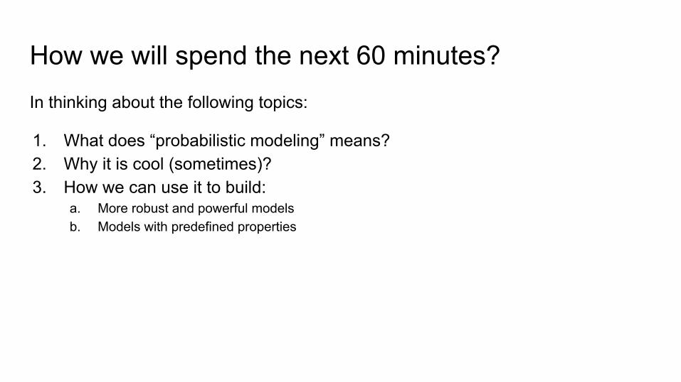
In thinking about the following topics:
1. What does “probabilistic modeling” means?
How we will spend the next 60 minutes?

In thinking about the following topics:
1. What does “probabilistic modeling” means?2. Why it is cool (sometimes)?
How we will spend the next 60 minutes?

In thinking about the following topics:
1. What does “probabilistic modeling” means?2. Why it is cool (sometimes)?3. How we can use it to build:
How we will spend the next 60 minutes?

In thinking about the following topics:
1. What does “probabilistic modeling” means?2. Why it is cool (sometimes)?3. How we can use it to build:
a. More robust and powerful models
How we will spend the next 60 minutes?
In thinking about the following topics:
1. What does “probabilistic modeling” means?2. Why it is cool (sometimes)?3. How we can use it to build:
a. More robust and powerful modelsb. Models with predefined properties
How we will spend the next 60 minutes?
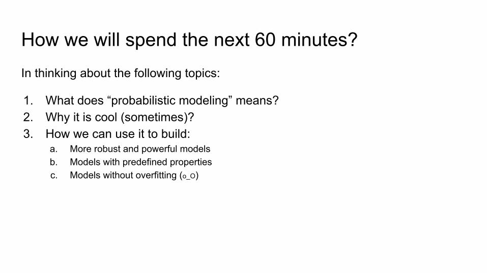
In thinking about the following topics:
1. What does “probabilistic modeling” means?2. Why it is cool (sometimes)?3. How we can use it to build:
a. More robust and powerful modelsb. Models with predefined propertiesc. Models without overfitting (o_O)
How we will spend the next 60 minutes?
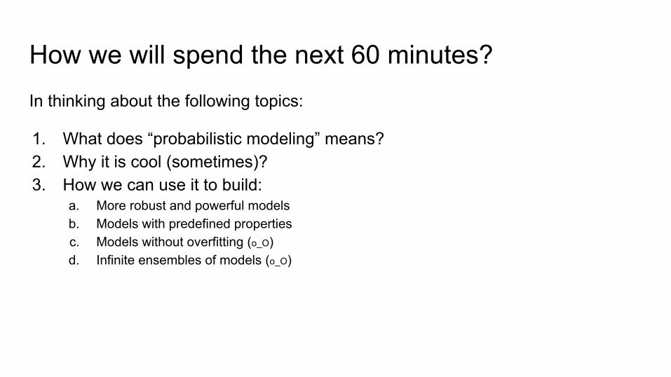
In thinking about the following topics:
1. What does “probabilistic modeling” means?2. Why it is cool (sometimes)?3. How we can use it to build:
a. More robust and powerful modelsb. Models with predefined propertiesc. Models without overfitting (o_O)d. Infinite ensembles of models (o_O)
4. Deep Learning
How we will spend the next 60 minutes?

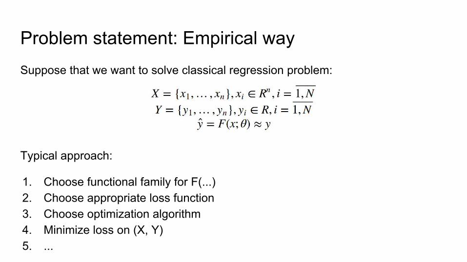
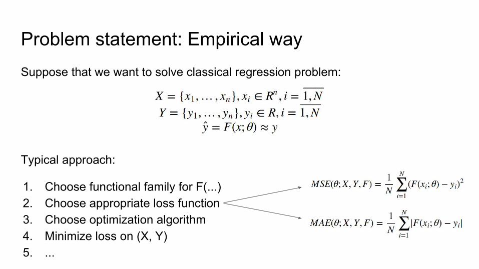
Problem statement: Empirical waySuppose that we want to solve classical regression problem:

Problem statement: Empirical waySuppose that we want to solve classical regression problem:
Typical approach:
Problem statement: Empirical waySuppose that we want to solve classical regression problem:
Typical approach:
1. Choose functional family for F(...)2. Choose appropriate loss function3. Choose optimization algorithm4. Minimize loss on (X, Y)5. ...
Problem statement: Empirical waySuppose that we want to solve classical regression problem:
Typical approach:
1. Choose functional family for F(...)2. Choose appropriate loss function3. Choose optimization algorithm4. Minimize loss on (X, Y)5. ...

Problem statement: Probabilistic wayDefine “probability model” (describes how your data was generated):

Problem statement: Probabilistic wayDefine “probability model” (describes how your data was generated):
Having model you can calculate “likelihood” of your data:

Problem statement: Probabilistic wayDefine “probability model” (describes how your data was generated):
Having model you can calculate “likelihood” of your data:
We are working with i.i.d. data

Problem statement: Probabilistic wayDefine “probability model” (describes how your data was generated):
Having model you can calculate “likelihood” of your data:
Sharing the same variance

Problem statement: Probabilistic wayData log-likelihood:
Maximum likelihood estimation:

Problem statement: Probabilistic wayData log-likelihood:
Maximum likelihood estimation:
MSE Loss minimization

Problem statement: Probabilistic wayData log-likelihood:
Maximum likelihood estimation:
MSE Loss minimizationFor i.i.d. data sharing the same variance!

Problem statement: Probabilistic way

Problem statement: Probabilistic way
Log-Likelihood maximization = Empirical loss minimization

Problem statement: Probabilistic way
1. MAE minimization = likelihood maximization of i.i.d. Laplace-distributed variables
Empirical loss minimizationLog-Likelihood maximization =

Problem statement: Probabilistic way
1. MAE minimization = likelihood maximization of i.i.d. Laplace-distributed variables2. For each empirically stated problem exists appropriate probability model
Empirical loss minimizationLog-Likelihood maximization =

Problem statement: Probabilistic way
1. MAE minimization = likelihood maximization of i.i.d. Laplace-distributed variables2. For each empirically stated problem exists appropriate probability model3. Empirical loss is often just a particular case of wider probability model
Empirical loss minimizationLog-Likelihood maximization =

Problem statement: Probabilistic way
1. MAE minimization = likelihood maximization of i.i.d. Laplace-distributed variables2. For each empirically stated problem exists appropriate probability model3. Empirical loss is often just a particular case of wider probability model4. Wider model = wider opportunities!
Empirical loss minimizationLog-Likelihood maximization =

Probabilistic modeling: Wider opportunities for FloSuppose that we have:
1. N unique users in the training set2. For each user we’ve collected time series of user states (on daily basis):
3. For each user we’ve collected time series of cycles lengths:
4. We predict time series of lengths Y based on time series of states X

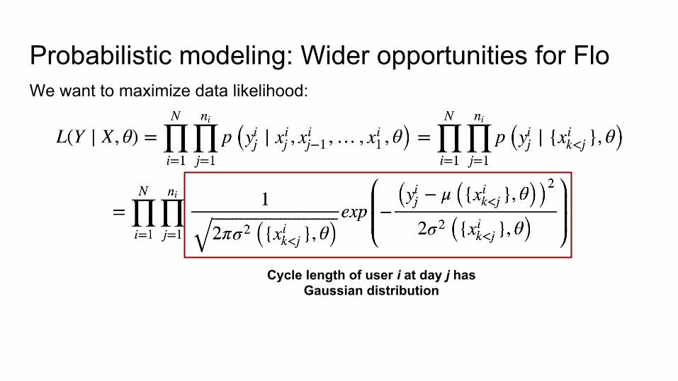
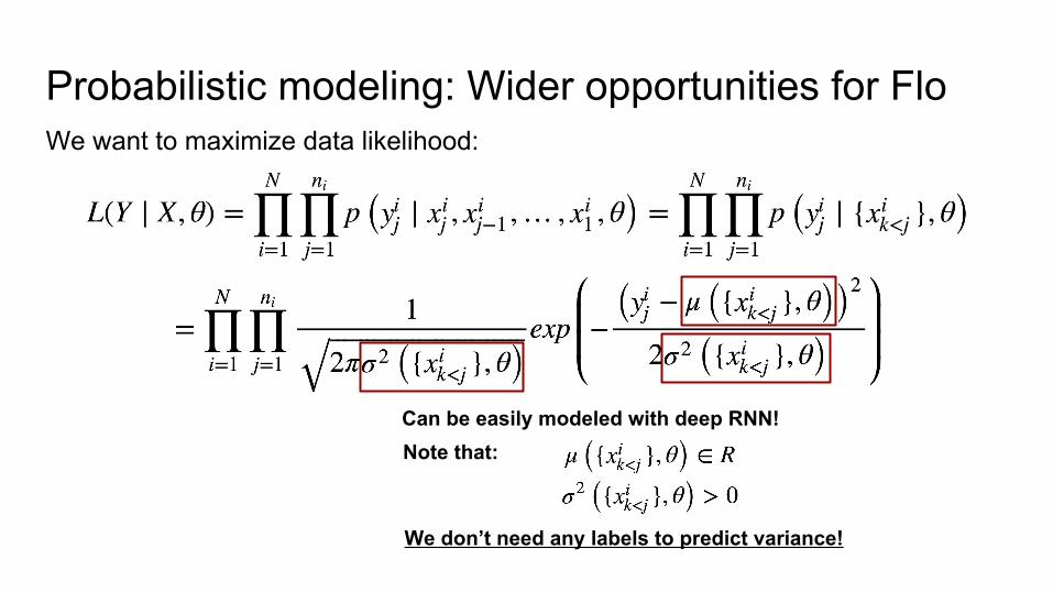
Probabilistic modeling: Wider opportunities for FloWe want to maximize data likelihood:

Probabilistic modeling: Wider opportunities for FloWe want to maximize data likelihood:
Probability that user i will have cycle with length y at day j

Probabilistic modeling: Wider opportunities for FloWe want to maximize data likelihood:
Just another notationProbability that user i will have cycle with length y at day j
Probabilistic modeling: Wider opportunities for FloWe want to maximize data likelihood:
Cycle length of user i at day j has Gaussian distribution
Probabilistic modeling: Wider opportunities for FloWe want to maximize data likelihood:
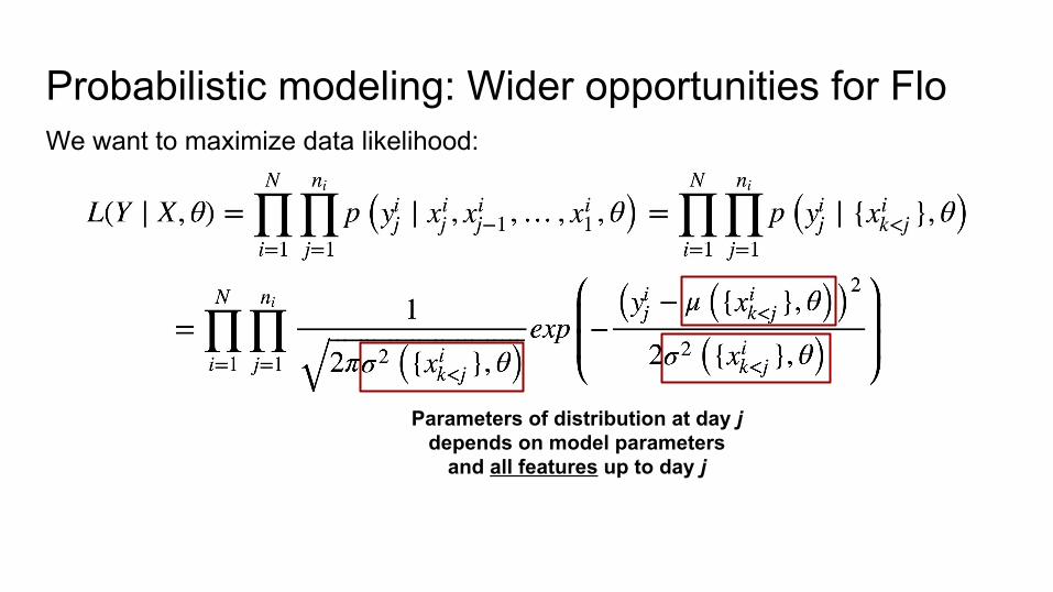
Parameters of distribution at day j depends on model parameters
and all features up to day j
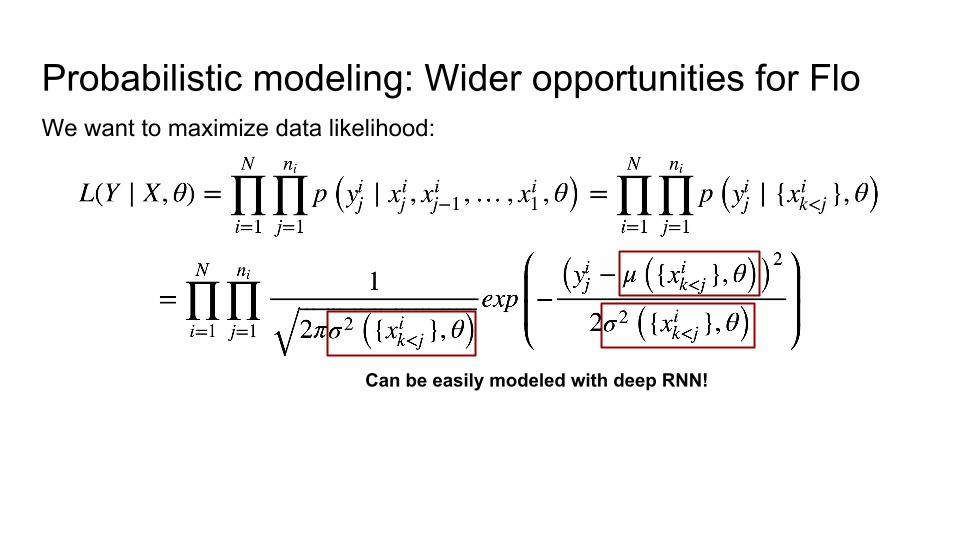
Probabilistic modeling: Wider opportunities for FloWe want to maximize data likelihood:
Can be easily modeled with deep RNN!

Probabilistic modeling: Wider opportunities for FloWe want to maximize data likelihood:
Can be easily modeled with deep RNN!Note that:
Probabilistic modeling: Wider opportunities for FloWe want to maximize data likelihood:
Can be easily modeled with deep RNN!Note that:
We don’t need any labels to predict variance!
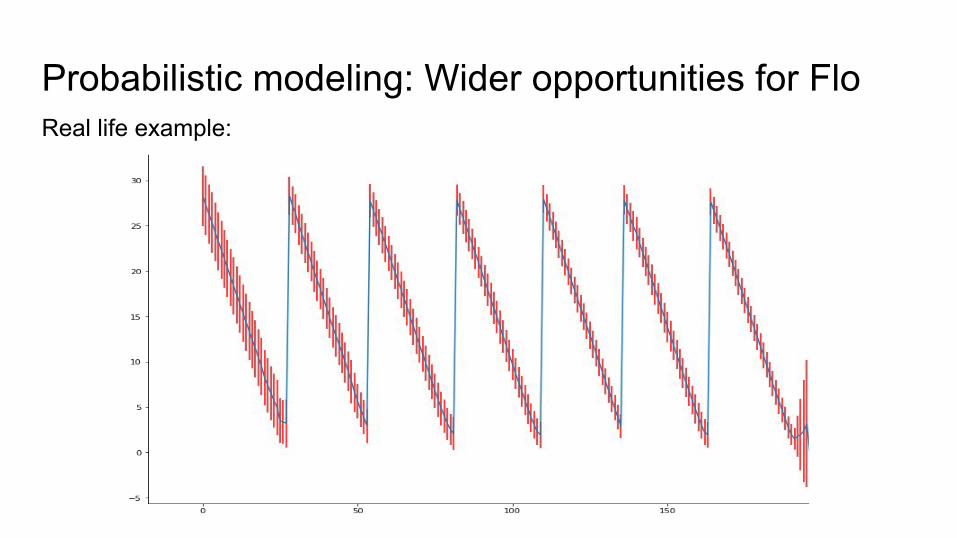
Probabilistic modeling: Wider opportunities for FloReal life example:

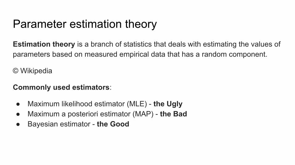
Parameter estimation theoryEstimation theory is a branch of statistics that deals with estimating the values of parameters based on measured empirical data that has a random component.
© Wikipedia
Parameter estimation theoryEstimation theory is a branch of statistics that deals with estimating the values of parameters based on measured empirical data that has a random component.
© Wikipedia
Commonly used estimators:
● Maximum likelihood estimator (MLE) - the Ugly● Maximum a posteriori estimator (MAP) - the Bad● Bayesian estimator - the Good
We are here

Parameter estimation theoryEstimation theory is a branch of statistics that deals with estimating the values of parameters based on measured empirical data that has a random component.
© Wikipedia
Commonly used estimators:
● Maximum likelihood estimator (MLE) - the Ugly● Maximum a posteriori estimator (MAP) - the Bad● Bayesian estimator - the Good
The way we go

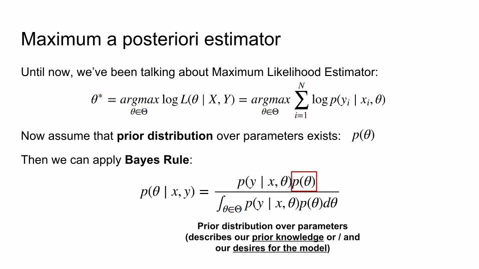
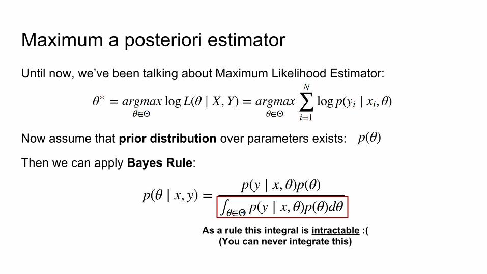
Maximum a posteriori estimatorUntil now, we’ve been talking about Maximum Likelihood Estimator:

Maximum a posteriori estimatorUntil now, we’ve been talking about Maximum Likelihood Estimator:
Now assume that prior distribution over parameters exists:

Maximum a posteriori estimatorUntil now, we’ve been talking about Maximum Likelihood Estimator:
Now assume that prior distribution over parameters exists:
Then we can apply Bayes Rule:

Maximum a posteriori estimatorUntil now, we’ve been talking about Maximum Likelihood Estimator:
Now assume that prior distribution over parameters exists:
Then we can apply Bayes Rule:
Posterior distributionover model parameters

Maximum a posteriori estimatorUntil now, we’ve been talking about Maximum Likelihood Estimator:
Now assume that prior distribution over parameters exists:
Then we can apply Bayes Rule:
Data likelihood for specific parameters(could be modeled with Deep Network!)
Maximum a posteriori estimatorUntil now, we’ve been talking about Maximum Likelihood Estimator:
Now assume that prior distribution over parameters exists:
Then we can apply Bayes Rule:
Prior distribution over parameters(describes our prior knowledge or / and
our desires for the model)

Maximum a posteriori estimatorUntil now, we’ve been talking about Maximum Likelihood Estimator:
Now assume that prior distribution over parameters exists:
Then we can apply Bayes Rule:
Bayesian evidence

Maximum a posteriori estimatorUntil now, we’ve been talking about Maximum Likelihood Estimator:
Now assume that prior distribution over parameters exists:
Then we can apply Bayes Rule:
Bayesian evidenceA powerful method for model selection!
Maximum a posteriori estimatorUntil now, we’ve been talking about Maximum Likelihood Estimator:
Now assume that prior distribution over parameters exists:
Then we can apply Bayes Rule:
As a rule this integral is intractable :((You can never integrate this)
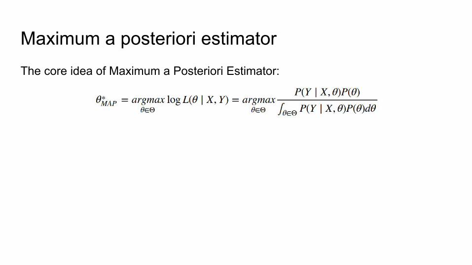
Maximum a posteriori estimatorThe core idea of Maximum a Posteriori Estimator:

Maximum a posteriori estimatorThe core idea of Maximum a Posteriori Estimator:
Doesn’t depend on model parameters

Maximum a posteriori estimatorThe core idea of Maximum a Posteriori Estimator:

Maximum a posteriori estimatorThe core idea of Maximum a Posteriori Estimator:
The only (but powerful!)difference from MLE

Maximum a posteriori estimatorThe core idea of Maximum a Posteriori Estimator:
1. MAP estimates model parameters as mode of posterior distribution

Maximum a posteriori estimatorThe core idea of Maximum a Posteriori Estimator:
1. MAP estimates model parameters as mode of posterior distribution2. MAP estimation with non-informative prior = MLE

Maximum a posteriori estimatorThe core idea of Maximum a Posteriori Estimator:
1. MAP estimates model parameters as mode of posterior distribution2. MAP estimation with non-informative prior = MLE3. MAP restricts the search space of possible models

Maximum a posteriori estimatorThe core idea of Maximum a Posteriori Estimator:
1. MAP estimates model parameters as mode of posterior distribution2. MAP estimation with non-informative prior = MLE3. MAP restricts the search space of possible models 4. With MAP you can put restrictions not only on model weights but also on many
interactions inside the network
Probabilistic modeling: RegularizationRegularization - is a process of introducing additional information in order to solve an ill-posed problem or prevent overfitting. © Wikipedia

Probabilistic modeling: RegularizationRegularization - is a process of introducing additional information in order to solve an ill-posed problem or prevent overfitting. © Wikipedia
Regularization - is a process of introducing additional information in order to restrict model to have predefined properties.
It is closely connected to “prior distributions” on weights / activations / …
… and to MAP estimation!

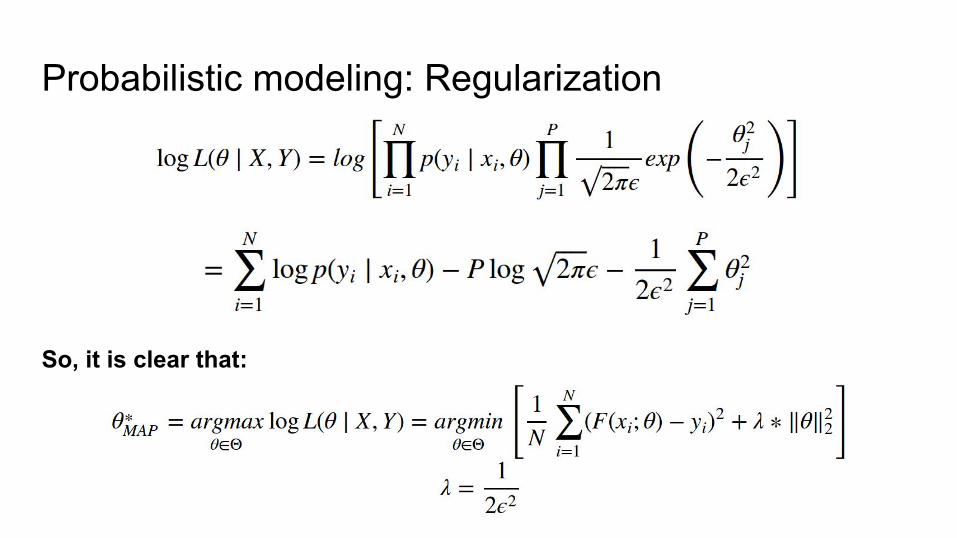
Probabilistic modeling: RegularizationWeights decay (or L2 regularization):

Probabilistic modeling: RegularizationWeights decay (or L2 regularization):
Appropriate probability model:
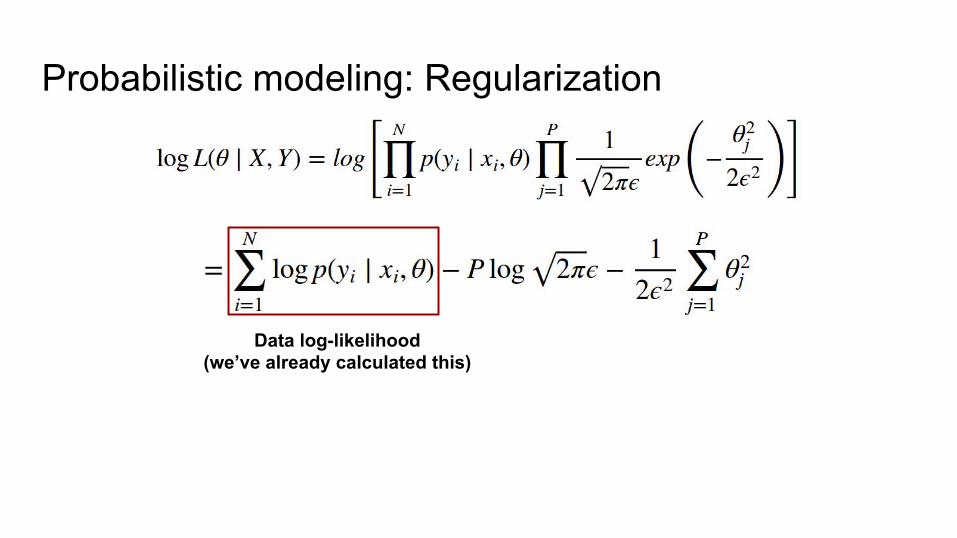
Model log-likelihood:

Probabilistic modeling: Regularization

Probabilistic modeling: Regularization
Probabilistic modeling: Regularization
Data log-likelihood(we’ve already calculated this)

Probabilistic modeling: Regularization
Doesn’t depend onmodel parameters

Probabilistic modeling: Regularization
Squared L2 normof parameters

Probabilistic modeling: Regularization
Regularization constant
Probabilistic modeling: Regularization
So, it is clear that:
Probabilistic modeling: Regularization1. Laplace distribution as a prior = L1 regularization

Probabilistic modeling: Regularization1. Laplace distribution as a prior = L1 regularization2. It can be shown that Dropout is also a form of particular probability model …

Probabilistic modeling: Regularization1. Laplace distribution as a prior = L1 regularization2. It can be shown that Dropout is also a form of particular probability model …3. … a Bayesian one :) …
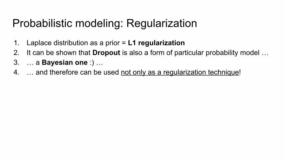
Probabilistic modeling: Regularization1. Laplace distribution as a prior = L1 regularization2. It can be shown that Dropout is also a form of particular probability model …3. … a Bayesian one :) …4. … and therefore can be used not only as a regularization technique!

Probabilistic modeling: Regularization1. Laplace distribution as a prior = L1 regularization2. It can be shown that Dropout is also a form of particular probability model …3. … a Bayesian one :) …4. … and therefore can be used not only as a regularization technique!5. Do you want to pack your network weights into few kilobytes?

Probabilistic modeling: Regularization1. Laplace distribution as a prior = L1 regularization2. It can be shown that Dropout is also a form of particular probability model …3. … a Bayesian one :) …4. … and therefore can be used not only as a regularization technique!5. Do you want to pack your network weights into few kilobytes?6. Ok, all you need - is MAP!

Probabilistic modeling: Regularization1. Laplace distribution as a prior = L1 regularization2. It can be shown that Dropout is also a form of particular probability model …3. … a Bayesian one :) …4. … and therefore can be used not only as a regularization technique!5. Do you want to pack your network weights into few kilobytes?6. Ok, all you need - is MAP!
MAP - is all you need!

Weights packing: Empirical way
Song Han and others - Deep Compression: Compressing Deep Neural Networks with Pruning, Trained Quantization and Huffman Coding (2015)
Modern neural networks could be dramatically compressed:
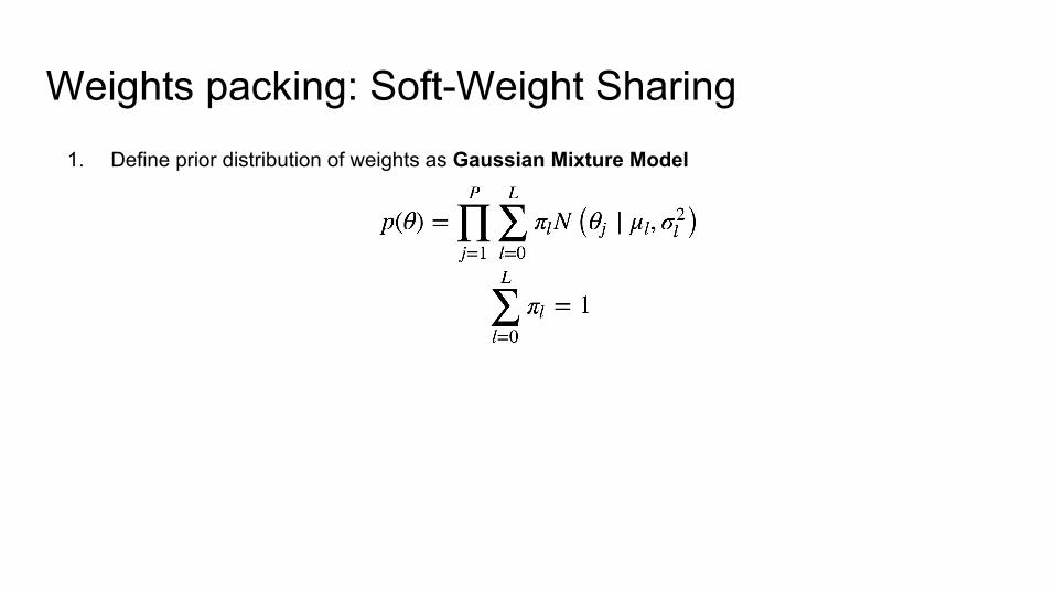
Weights packing: Soft-Weight Sharing1. Define prior distribution of weights as Gaussian Mixture Model
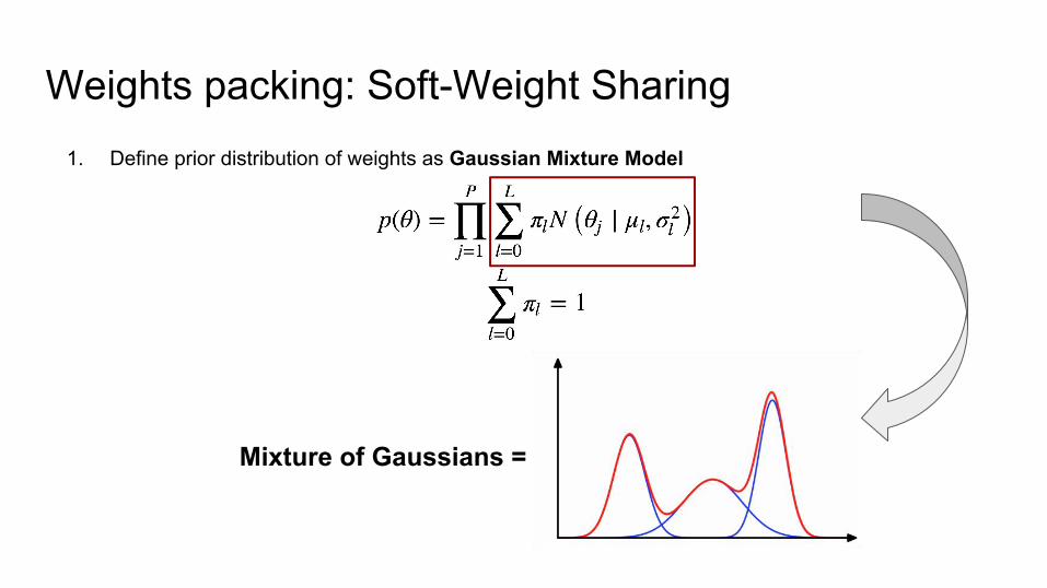
1. Define prior distribution of weights as Gaussian Mixture Model
Mixture of Gaussians =
Weights packing: Soft-Weight Sharing
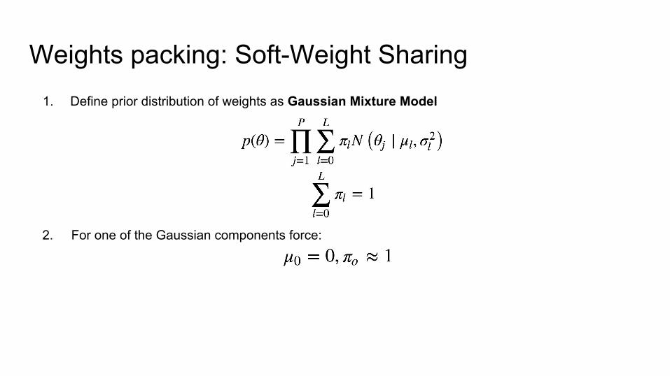
1. Define prior distribution of weights as Gaussian Mixture Model
2. For one of the Gaussian components force:
Weights packing: Soft-Weight Sharing
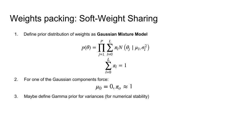
1. Define prior distribution of weights as Gaussian Mixture Model
2. For one of the Gaussian components force:
3. Maybe define Gamma prior for variances (for numerical stability)
Weights packing: Soft-Weight Sharing

1. Define prior distribution of weights as Gaussian Mixture Model
2. For one of the Gaussian components force:
3. Maybe define Gamma prior for variances (for numerical stability)
4. Just find MAP estimation for both model parameters and free mixture parameters!
Weights packing: Soft-Weight Sharing

Karen Ullrich - Soft Weight-Sharing For Neural Network Compression (2017)
Weights packing: Soft-Weight Sharing
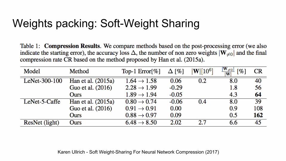
Karen Ullrich - Soft Weight-Sharing For Neural Network Compression (2017)
Weights packing: Soft-Weight Sharing

Maximum a posteriori estimation1. Pretty cool and powerful technique2. You can build hierarchical models (put priors on priors of priors of…)3. You can put priors on activations of layers (sparse autoencoders)4. Leads to “Empirical Bayes”5. Thinking how to restrict your model? Try to find appropriate prior!
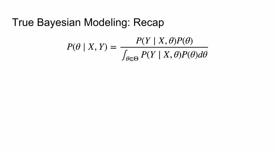
True Bayesian Modeling: Recap

True Bayesian Modeling: Recap
1. Posterior could be easily found in case of conjugate distributions

True Bayesian Modeling: Recap
1. Posterior could be easily found in case of conjugate distributions2. But for most real life models denominator is intractable

True Bayesian Modeling: Recap
1. Posterior could be easily found in case of conjugate distributions2. But for most real life models denominator is intractable3. In MAP denominator is totally ignored

True Bayesian Modeling: Recap
1. Posterior could be easily found in case of conjugate distributions2. But for most real life models denominator is intractable3. In MAP denominator is totally ignored4. Can we find a good approximation of the posterior?
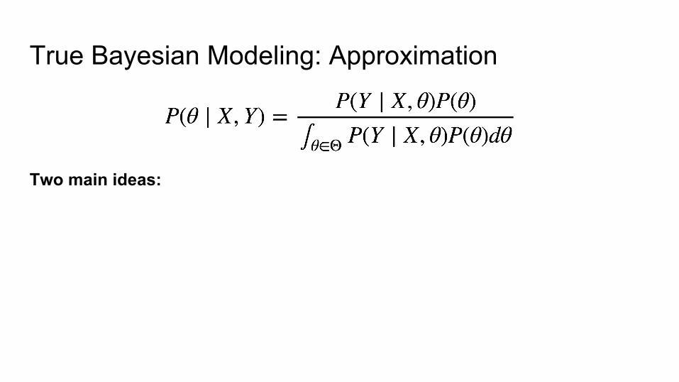
True Bayesian Modeling: Approximation
Two main ideas:

True Bayesian Modeling: Approximation
Two main ideas:
1. MCMC (Monte Carlo Markov Chain)

True Bayesian Modeling: Approximation
Two main ideas:
1. MCMC (Monte Carlo Markov Chain) - a tricky one

True Bayesian Modeling: Approximation
Two main ideas:
1. MCMC (Monte Carlo Markov Chain) - a tricky one2. Variational Inference
True Bayesian Modeling: Approximation
Two main ideas:
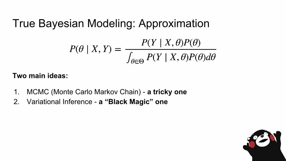
1. MCMC (Monte Carlo Markov Chain) - a tricky one2. Variational Inference - a “Black Magic” one

True Bayesian Modeling: Approximation
Two main ideas:
1. MCMC (Monte Carlo Markov Chain) - a tricky one2. Variational Inference - a “Black Magic” oneAnother ideas exists:
1. Monte Carlo Dropout2. Stochastic gradient langevin dynamics3. ...

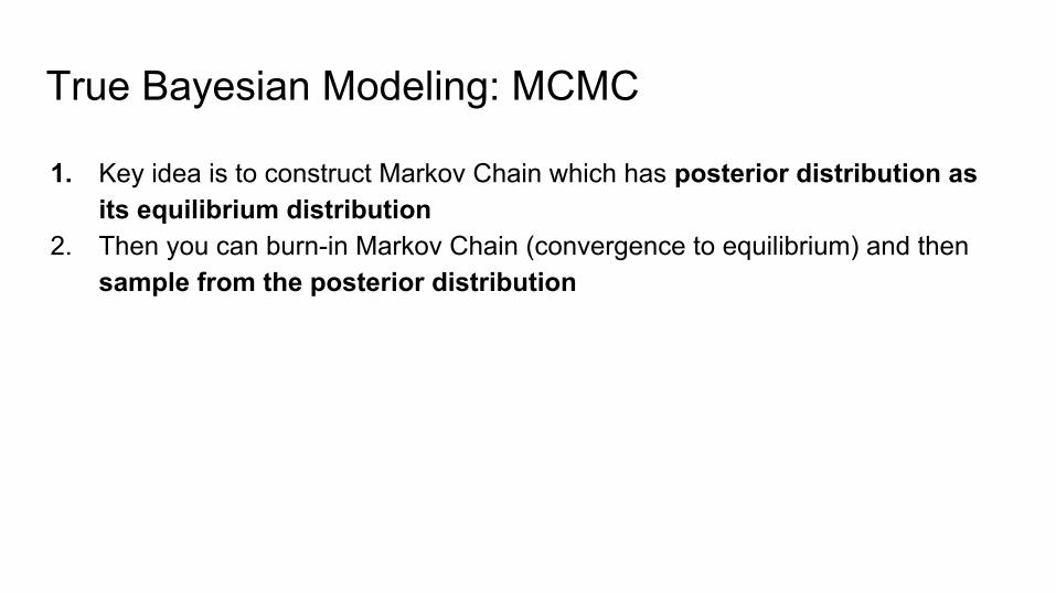
True Bayesian Modeling: MCMC
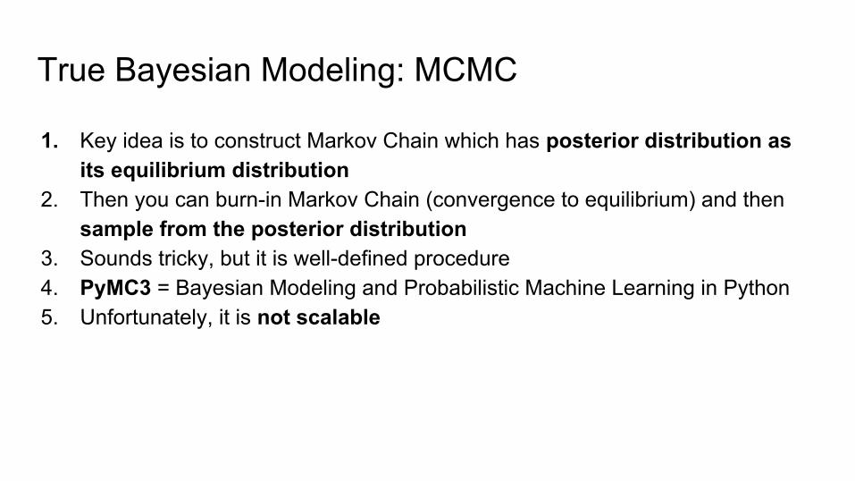
1. Key idea is to construct Markov Chain which has posterior distribution as its equilibrium distribution
True Bayesian Modeling: MCMC
1. Key idea is to construct Markov Chain which has posterior distribution as its equilibrium distribution
2. Then you can burn-in Markov Chain (convergence to equilibrium) and then sample from the posterior distribution

True Bayesian Modeling: MCMC
1. Key idea is to construct Markov Chain which has posterior distribution as its equilibrium distribution
2. Then you can burn-in Markov Chain (convergence to equilibrium) and then sample from the posterior distribution
3. Sounds tricky, but it is well-defined procedure

True Bayesian Modeling: MCMC
1. Key idea is to construct Markov Chain which has posterior distribution as its equilibrium distribution
2. Then you can burn-in Markov Chain (convergence to equilibrium) and then sample from the posterior distribution
3. Sounds tricky, but it is well-defined procedure4. PyMC3 = Bayesian Modeling and Probabilistic Machine Learning in Python
True Bayesian Modeling: MCMC
1. Key idea is to construct Markov Chain which has posterior distribution as its equilibrium distribution
2. Then you can burn-in Markov Chain (convergence to equilibrium) and then sample from the posterior distribution
3. Sounds tricky, but it is well-defined procedure4. PyMC3 = Bayesian Modeling and Probabilistic Machine Learning in Python5. Unfortunately, it is not scalable

True Bayesian Modeling: MCMC
1. Key idea is to construct Markov Chain which has posterior distribution as its equilibrium distribution
2. Then you can burn-in Markov Chain (convergence to equilibrium) and then sample from the posterior distribution
3. Sounds tricky, but it is well-defined procedure4. PyMC3 = Bayesian Modeling and Probabilistic Machine Learning in Python5. Unfortunately, it is not scalable6. So, you can’t explicitly apply it to complex models (like Neural Networks)

True Bayesian Modeling: MCMC
1. Key idea is to construct Markov Chain which has posterior distribution as its equilibrium distribution
2. Then you can burn-in Markov Chain (convergence to equilibrium) and then sample from the posterior distribution
3. Sounds tricky, but it is well-defined procedure4. PyMC3 = Bayesian Modeling and Probabilistic Machine Learning in Python5. Unfortunately, it is not scalable6. So, you can’t explicitly apply it to complex models (like Neural Networks)7. But implicit scaling is possible: Bayesian learning via stochastic gradient
langevin dynamics (2011)

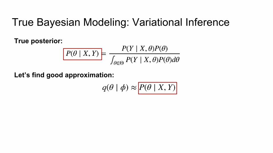
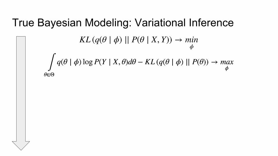
True Bayesian Modeling: Variational InferenceTrue posterior:

True Bayesian Modeling: Variational InferenceTrue posterior:
Modeled with Deep Neural Network

True Bayesian Modeling: Variational InferenceTrue posterior:
Intractable integral :(

True Bayesian Modeling: Variational InferenceTrue posterior:
Let’s find good approximation:
True Bayesian Modeling: Variational InferenceTrue posterior:
Let’s find good approximation:

True Bayesian Modeling: Variational InferenceTrue posterior:
Let’s find good approximation:
Explicitly define distribution familyfor approximation
(e.g. multivariate gaussian)

True Bayesian Modeling: Variational InferenceTrue posterior:
Let’s find good approximation:
Variational parameters(e.g. mean vector, covariance matrix)

True Bayesian Modeling: Variational InferenceTrue posterior:
Let’s find good approximation:
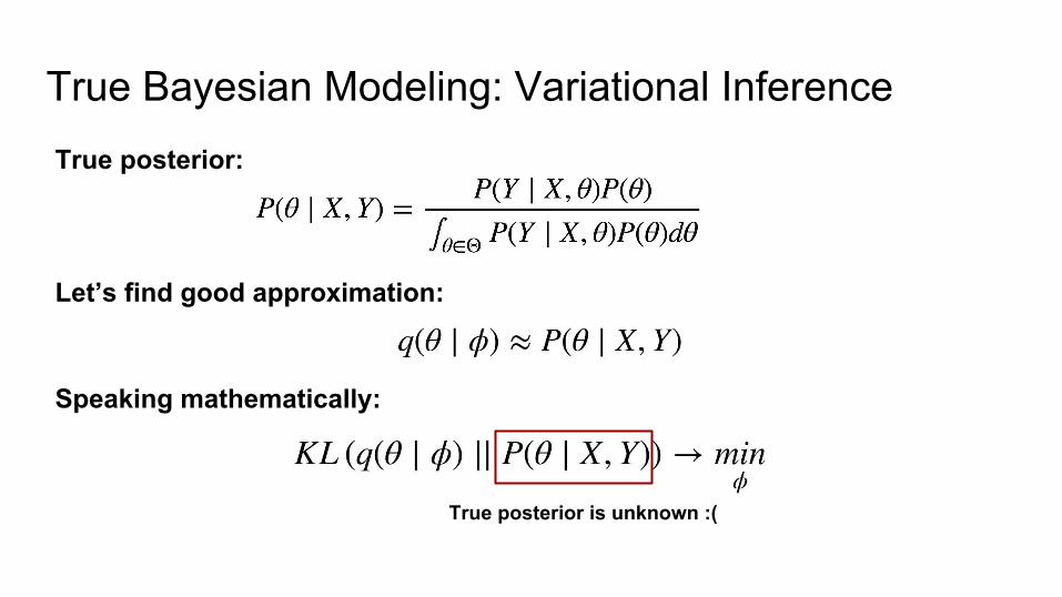
Speaking mathematically:

True Bayesian Modeling: Variational InferenceTrue posterior:
Let’s find good approximation:
Speaking mathematically:
Kullback-Leibler divergence(measure of distributions dissimilarity)
True Bayesian Modeling: Variational InferenceTrue posterior:
Let’s find good approximation:
Speaking mathematically:
True posterior is unknown :(

Achtung!A lot of math
is coming!

True Bayesian Modeling: Variational Inference

True Bayesian Modeling: Variational Inference

True Bayesian Modeling: Variational Inference

True Bayesian Modeling: Variational Inference
Rewrite this usingBayes rule:

True Bayesian Modeling: Variational Inference

True Bayesian Modeling: Variational Inference
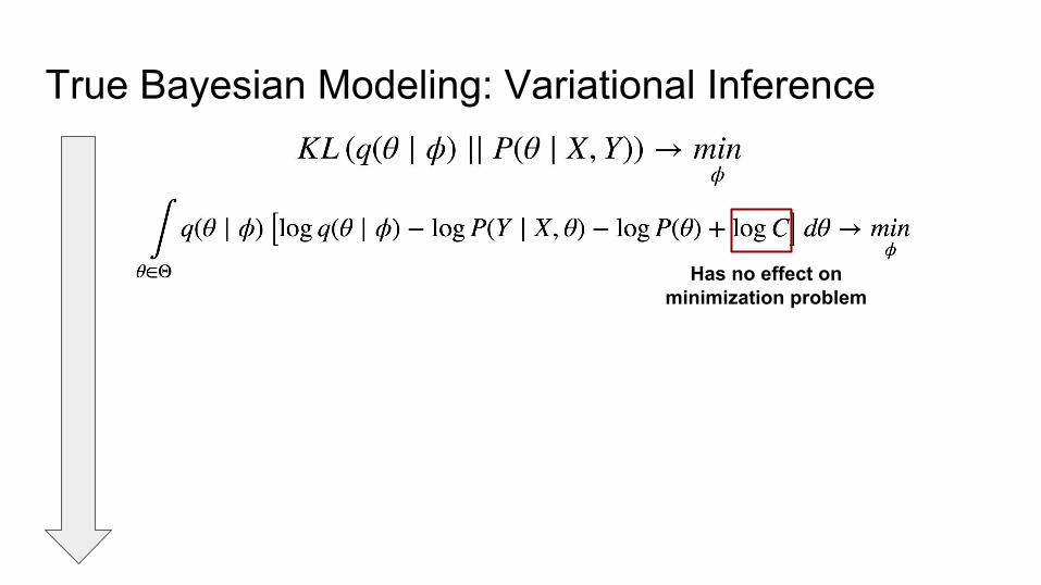
Doesn’t depend on theta!(After integration)
Parametersof integration

True Bayesian Modeling: Variational Inference
So, it is a constant!

True Bayesian Modeling: Variational Inference
True Bayesian Modeling: Variational Inference
Has no effect onminimization problem

True Bayesian Modeling: Variational Inference

True Bayesian Modeling: Variational Inference
Group this together

True Bayesian Modeling: Variational Inference

True Bayesian Modeling: Variational Inference
Multiply by (-1)

True Bayesian Modeling: Variational Inference

True Bayesian Modeling: Variational Inference
KLdivergence
True Bayesian Modeling: Variational Inference

True Bayesian Modeling: Variational Inference
It is an expectationover q(...)

True Bayesian Modeling: Variational Inference

True Bayesian Modeling: Variational Inference
Equivalent problems!

True Bayesian Modeling: Variational Inference
Equivalent problems!
Likelihood of your data(your Neural Network works here!)

True Bayesian Modeling: Variational Inference
Equivalent problems!
Prior on network weights(you define this!)

True Bayesian Modeling: Variational Inference
Equivalent problems!
Approximate posterior(you define the form of this!)

True Bayesian Modeling: Variational Inference
Equivalent problems!
We want to optimize this wrt of approximate posterior parameters!

True Bayesian Modeling: Variational Inference
Equivalent problems!
We need to calculate the gradient of this

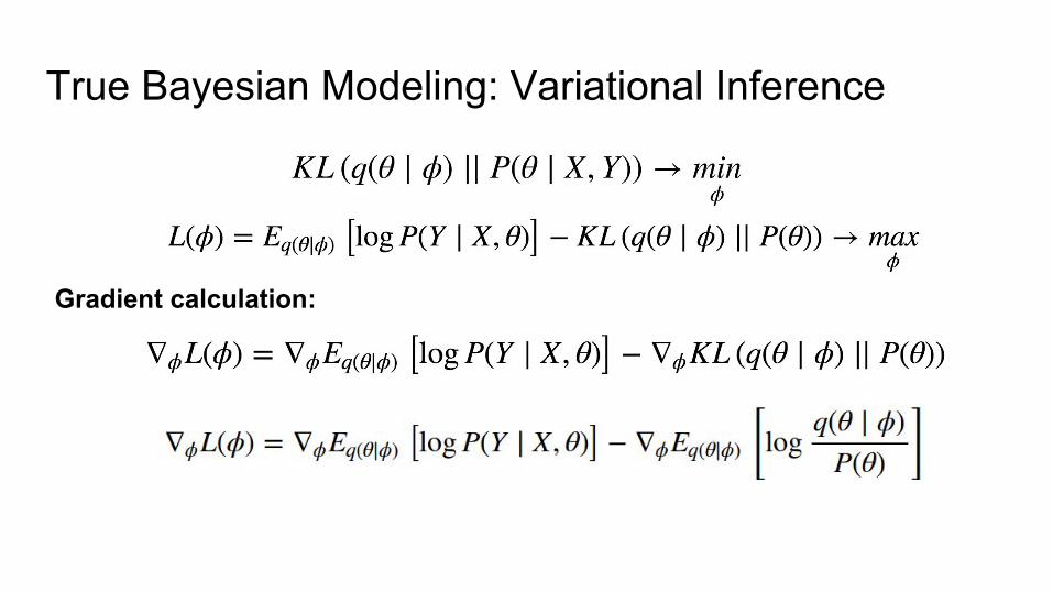
True Bayesian Modeling: Variational Inference
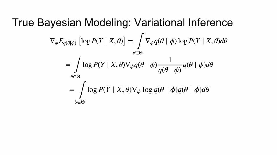
Gradient calculation:

True Bayesian Modeling: Variational Inference
Gradient calculation:

True Bayesian Modeling: Variational Inference
Gradient calculation:
Rewrite this as expectation(for convenience)
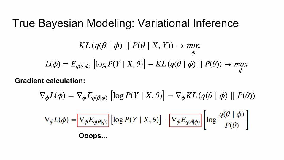
True Bayesian Modeling: Variational Inference
Gradient calculation:
True Bayesian Modeling: Variational Inference
Gradient calculation:
Ooops...
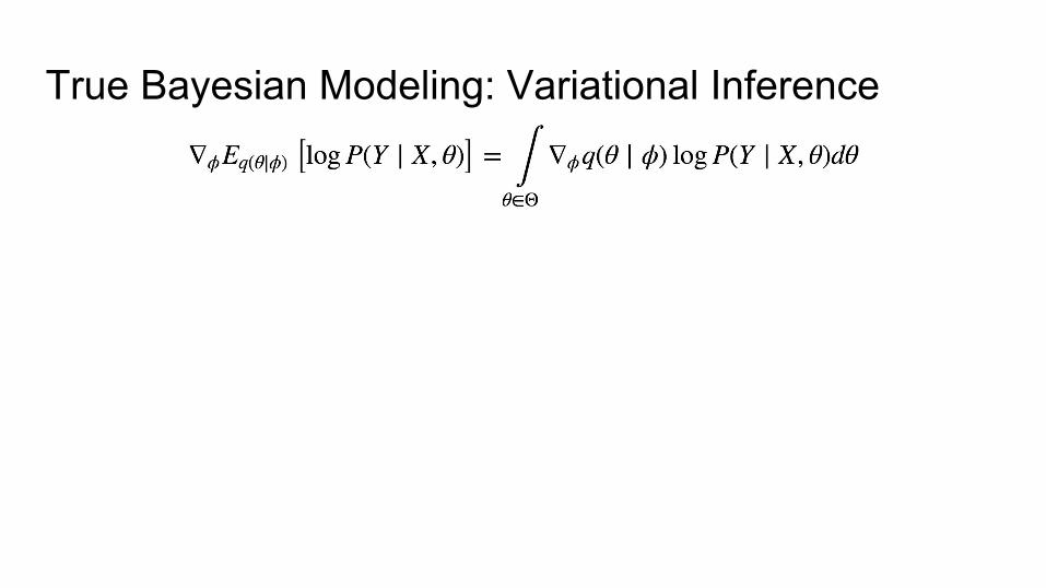
True Bayesian Modeling: Variational Inference

True Bayesian Modeling: Variational Inference
Modeled withDeep Network!

True Bayesian Modeling: Variational Inference
This integral is intractable too :((God damn!)

True Bayesian Modeling: Variational Inference
If it was just q(...) then we can calculate approximation using Monte Carlo
method!

True Bayesian Modeling: Variational Inference

True Bayesian Modeling: Variational Inference
This is just = 1!

True Bayesian Modeling: Variational Inference
This is gradient of log(q(...))!
True Bayesian Modeling: Variational Inference

True Bayesian Modeling: Variational Inference
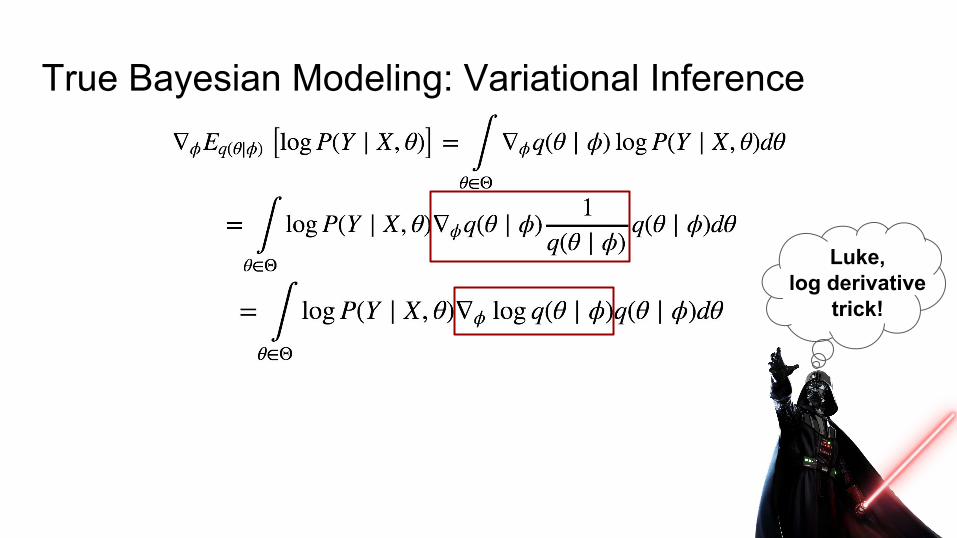
True Bayesian Modeling: Variational Inference
Luke,log derivative
trick!

True Bayesian Modeling: Variational Inference
Luke,log derivative
trick!

True Bayesian Modeling: Variational Inference
Can be approximatedwith Monte Carlo!
Luke,log derivative
trick!

True Bayesian Modeling: Variational Inference
Luke,log derivative
trick!

Bayesian Networks: Step by stepDefine functional family for approximate posterior (e.g. Gaussian):

Bayesian Networks: Step by stepDefine functional family for approximate posterior (e.g. Gaussian):
Solve optimization problem (with doubly stochastic gradient ascend):

Bayesian Networks: Step by stepDefine functional family for approximate posterior (e.g. Gaussian):
Solve optimization problem (with doubly stochastic gradient ascend):
Having approximate posterioryou can sample network weights (as much as you want)!
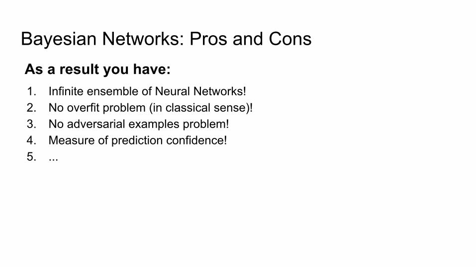
Bayesian Networks: Pros and ConsAs a result you have:1. Infinite ensemble of Neural Networks!2. No overfit problem (in classical sense)!3. No adversarial examples problem!4. Measure of prediction confidence!5. ...

Bayesian Networks: Pros and ConsAs a result you have:1. Infinite ensemble of Neural Networks!2. No overfit problem (in classical sense)!3. No adversarial examples problem!4. Measure of prediction confidence!5. ...
No free hunch:1. A lot of work is still hidden in “scalability” and “convergence”!2. Very (very!) expensive predictions!

Bayesian Networks Examples: BRNN
Meire Fortunato and others - Bayesian Recurrent Neural Networks (2017)

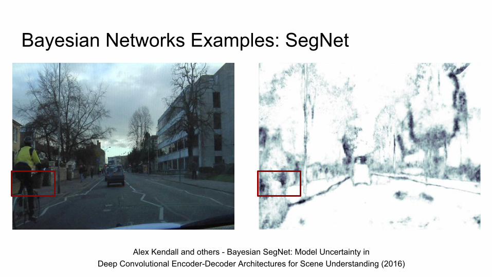
Bayesian Networks Examples: SegNet
Alex Kendall and others - Bayesian SegNet: Model Uncertainty inDeep Convolutional Encoder-Decoder Architectures for Scene Understanding (2016)

Bayesian Networks Examples: SegNet
Alex Kendall and others - Bayesian SegNet: Model Uncertainty inDeep Convolutional Encoder-Decoder Architectures for Scene Understanding (2016)

Bayesian Networks Examples: SegNet
Alex Kendall and others - Bayesian SegNet: Model Uncertainty inDeep Convolutional Encoder-Decoder Architectures for Scene Understanding (2016)

Bayesian Networks Examples: SegNet
Alex Kendall and others - Bayesian SegNet: Model Uncertainty inDeep Convolutional Encoder-Decoder Architectures for Scene Understanding (2016)
Bayesian Networks Examples: SegNet
Alex Kendall and others - Bayesian SegNet: Model Uncertainty inDeep Convolutional Encoder-Decoder Architectures for Scene Understanding (2016)

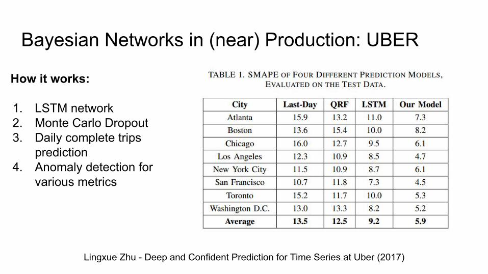
Bayesian Networks in (near) Production: UBER
Lingxue Zhu - Deep and Confident Prediction for Time Series at Uber (2017)
How it works:
1. LSTM network2. Monte Carlo Dropout3. Daily complete trips
prediction4. Anomaly detection for
various metrics
Bayesian Networks in (near) Production: UBER
Lingxue Zhu - Deep and Confident Prediction for Time Series at Uber (2017)
How it works:
1. LSTM network2. Monte Carlo Dropout3. Daily complete trips
prediction4. Anomaly detection for
various metrics

Bayesian Networks in (near) Production: UBER
Lingxue Zhu - Deep and Confident Prediction for Time Series at Uber (2017)
How it works:
1. LSTM network2. Monte Carlo Dropout3. Daily complete trips
prediction4. Anomaly detection for
various metrics

Bayesian Networks in (near) Production: Flo
Predicted distributions of cycle length for 40 independent users:
Switched to Empirical Bayes for now.

Speech Summary
1. Probabilistic modeling is a powerful tool with strong math background

Speech Summary
1. Probabilistic modeling is a powerful tool with strong math background2. Many techniques are currently not widely used in Deep Learning

Speech Summary
1. Probabilistic modeling is a powerful tool with strong math background2. Many techniques are currently not widely used in Deep Learning3. You can improve many aspects of your model using the same framework

Speech Summary
1. Probabilistic modeling is a powerful tool with strong math background2. Many techniques are currently not widely used in Deep Learning3. You can improve many aspects of your model using the same framework4. Scalability, stability of convergence and inference cost are main constraints

Speech Summary
1. Probabilistic modeling is a powerful tool with strong math background2. Many techniques are currently not widely used in Deep Learning3. You can improve many aspects of your model using the same framework4. Scalability, stability of convergence and inference cost are main constraints5. The future of Deep Learning looks Bayesian...
… (for the moment, for me)
Thank you for your !
I hope, you have a lot of questions :)
(attention)
Dzianis DusLead Data Scientist at InData Labs