probabilistic programming - github pages
TRANSCRIPT

Probabilistic ProgrammingAn Emerging Field
ML: Algorithms &Applications
STATS: Inference &
Theory
PL: Compilers,Semantics,
Analysis
ProbabilisticProgramming
Figure credit: Frank Wood
Why Probabilistic Programming?
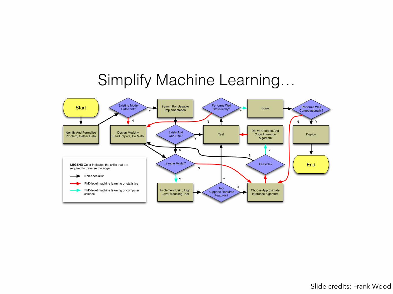
Simplify Machine Learning…Start
Identify And Formalize Problem, Gather Data
Design Model = Read Papers, Do Math
Existing Model Sufficient?
Choose Approximate Inference Algorithm
Derive Updates And Code Inference
Algorithm
Exists AndCan Use?
Performs Well Statistically?
End
Performs Well Computationally?
Search For Useable Implementation
Test
Scale
Deploy
Simple Model?
Implement Using High Level Modeling Tool
ToolSupports Required
Features?
N
N
N
N
N N
Y
Y Y
Y
Y
Y
LEGEND Color indicates the skills that are required to traverse the edge.
PhD-level machine learning or statistics
PhD-level machine learning or computer science
Non-specialist
Feasible?
YN
Slide credits: Frank Wood

To ThisStart
Identify And Formalize Problem, Gather Data
Design Model = Write Probabilistic
Program
Existing Model Sufficient?
Derive Updates And Code Inference
Algorithm
Exists AndCan Use?
Performs Well?
End
Performs Well Computationally?
Search For Useable Implementation
Debug, Test, Profile
Scale
Deploy
N Y
LEGEND Color indicates the skills that are required to traverse the edge.
Non-specialist
Choose Approximate Inference Algorithm
Simple Model?
Implement Using High Level Modeling Tool
ToolSupports Required
Features?
Feasible?
Slide credits: Frank Wood
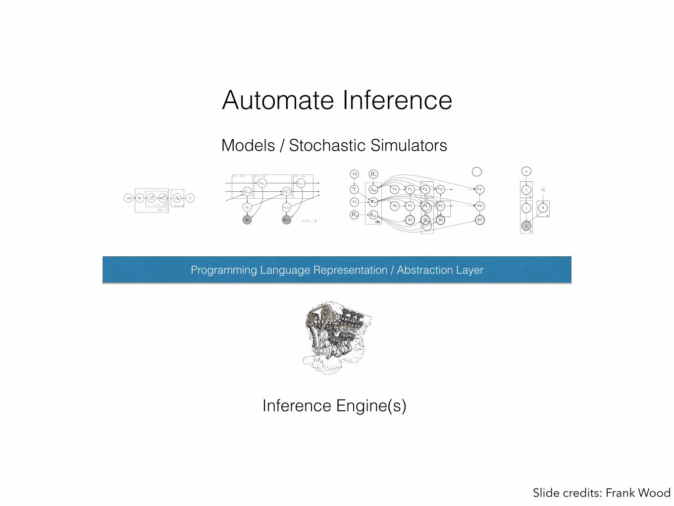
Slide credits: Frank Wood
Automate Inference
Programming Language Representation / Abstraction Layer
Inference Engine(s)
Models / Stochastic Simulators
CARON ET AL.
This lack of consistency is shared by other models based on the Polya urn construction (Zhuet al., 2005; Ahmed and Xing, 2008; Blei and Frazier, 2011). Blei and Frazier (2011) provide adetailed discussion on this issue and describe cases where one should or should not bother about it.
It is possible to define a slightly modified version of our model that is consistent under marginal-isation, at the expense of an additional set of latent variables. This is described in Appendix C.
3.2 Stationary Models for Cluster Locations
To ensure we obtain a first-order stationary Pitman-Yor process mixture model, we also need tosatisfy (B). This can be easily achieved if for k 2 I(mt
t)
Uk,t ⇠⇢
p (·|Uk,t�1) if k 2 I(mtt�1)
H otherwise
where H is the invariant distribution of the Markov transition kernel p (·|·). In the time seriesliterature, many approaches are available to build such transition kernels based on copulas (Joe,1997) or Gibbs sampling techniques (Pitt and Walker, 2005).
Combining the stationary Pitman-Yor and cluster locations models, we can summarize the fullmodel by the following Bayesian network in Figure 1. It can also be summarized using a Chineserestaurant metaphor (see Figure 2).
Figure 1: A representation of the time-varying Pitman-Yor process mixture as a directed graphi-cal model, representing conditional independencies between variables. All assignmentvariables and observations at time t are denoted ct and zt, respectively.
3.3 Properties of the Models
Under the uniform deletion model, the number At =P
imti,t�1 of alive allocation variables at time
t can be written as
At =t�1X
j=1
nX
k=1
Xj,k
8
c0 Hr
� �m
c1 ⇡m
Hy ✓m
r0
s0
r1
s1
y1
r2
s2
y2
rT
sT
yT
r3
s3
y31
Gaussian Mixture Model
¼
µc
yi
k
k
i
N
K
K
α
Gπ
θc
yi
k
k o
i
N
K
K
α
Gπ
θc
yi
k
k o
i
N
1
1
Figure : From left to right: graphical models for a finite Gaussian mixture model(GMM), a Bayesian GMM, and an infinite GMM
ci |~⇡ ⇠ Discrete(~⇡)
~yi |ci = k ;⇥ ⇠ Gaussian(·|✓k).
~⇡|↵ ⇠ Dirichlet(·| ↵K
, . . . ,↵
K)
⇥ ⇠ G0
Wood (University of Oxford) Unsupervised Machine Learning January, 2014 16 / 19
Latent Dirichlet Allocation
↵ wdizd
i �k �
d = 1 . . . D
i = 1 . . . Nd.
✓d
k = 1 . . . K
Figure 1. Graphical model for LDA model
Lecture LDA
LDA is a hierarchical model used to model text documents. Each document is modeled asa mixture of topics. Each topic is defined as a distribution over the words in the vocabulary.Here, we will denote by K the number of topics in the model. We use D to indicate thenumber of documents, M to denote the number of words in the vocabulary, and Nd
. todenote the number of words in document d. We will assume that the words have beentranslated to the set of integers {1, . . . , M} through the use of a static dictionary. This isfor convenience only and the integer mapping will contain no semantic information. Thegenerative model for the D documents can be thought of as sequentially drawing a topicmixture ✓d for each document independently from a DirK(↵~1) distribution, where DirK(~�)is a Dirichlet distribution over the K-dimensional simplex with parameters [�1, �2, . . . , �K ].Each of K topics {�k}K
k=1 are drawn independently from DirM (�~1). Then, for each of thei = 1 . . . Nd. words in document d, an assignment variable zd
i is drawn from Mult(✓d).Conditional on the assignment variable zd
i , word i in document d, denoted as wdi , is drawn
independently from Mult(�zdi). The graphical model for the process can be seen in Figure 1.
The model is parameterized by the vector valued parameters {✓d}Dd=1, and {�k}K
k=1, theparameters {Zd
i }d=1,...,D,i=1,...,Nd., and the scalar positive parameters ↵ and �. The model
is formally written as:
✓d ⇠ DirK(↵~1)
�k ⇠ DirM (�~1)
zdi ⇠ Mult(✓d)
wdi ⇠ Mult(�zd
i)
1
✓d ⇠ DirK (↵~1)
�k ⇠ DirM(�~1)
zdi ⇠ Discrete(✓d)
wdi ⇠ Discrete(�zdi
)
Wood (University of Oxford) Unsupervised Machine Learning January, 2014 15 / 19
What is Probabilistic Programming?
Operative Definition“Probabilistic programs are usual functional or imperative programs with two added constructs:
(1) the ability to draw values at random from distributions, and
(2) the ability to condition values of variables in a program via observations.”
Gordon et al, 2014
Slide credits: Frank Wood

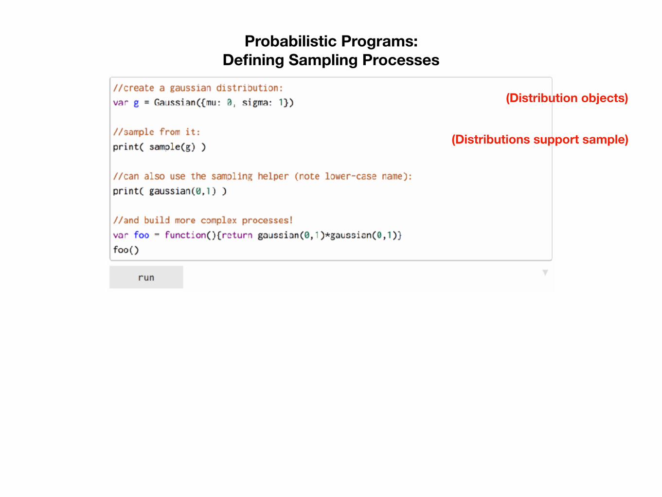
Probabilistic Programs: Defining Sampling Processes

(Distribution objects)
Probabilistic Programs: Defining Sampling Processes
(Distribution objects)
(Distributions support sample)
Probabilistic Programs: Defining Sampling Processes

(Distribution objects)
(Distributions support sample)
(Easy to build complex distributions)
Probabilistic Programs: Defining Sampling Processes

Probabilistic Programs: Defining Sampling Processes

Probabilistic Programs: Defining Sampling Processes
The generative model is now defined by a sampling process
A sampling process implicitly defines a distribution over output values…
Another PPL construct makes this distribution explicit: Infer
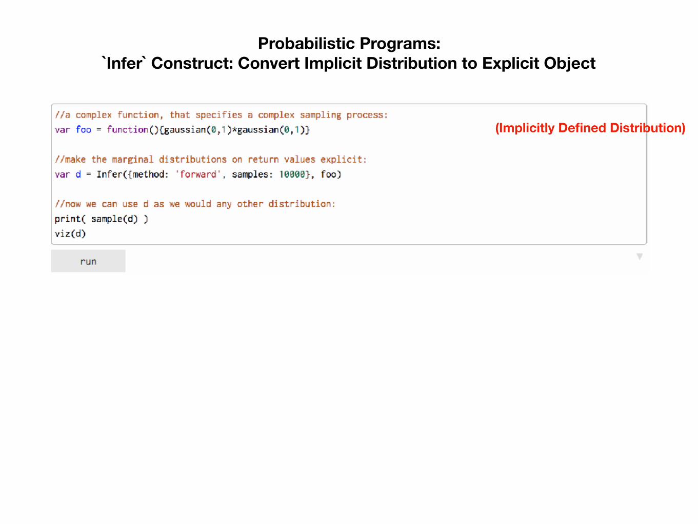
Probabilistic Programs: `Infer` Construct: Convert Implicit Distribution to Explicit Object
(Implicitly Defined Distribution)

Probabilistic Programs: `Infer` Construct: Convert Implicit Distribution to Explicit Object
(Implicitly Defined Distribution)
(Infer by Forward Sampling)

Probabilistic Programs: `Infer` Construct: Convert Implicit Distribution to Explicit Object
(Implicitly Defined Distribution)
(Infer by Forward Sampling)
(Now Use like Distribution Object)

Probabilistic Programs: `Infer` Construct: Convert Implicit Distribution to Explicit Object

Need one more language feature: “mem” `Random but persistent`: random on first call,
cached for subsequent calls Why needed:
Call once

Need one more language feature: “mem” `Random but persistent`: random on first call,
cached for subsequent calls Why needed:
Call onceCall twice

Need one more language feature: “mem” `Random but persistent`: random on first call,
cached for subsequent calls Why needed:
Bob’s eye color shouldn’t change…
Call onceCall twice

Need one more language feature: `mem` `Random but persistent`: random on first call,
cached for subsequent calls Why needed:
Call onceCall twice
Fixed: value is memoized after first run

Aside: Dirichlet Process as
Probabilistic Program
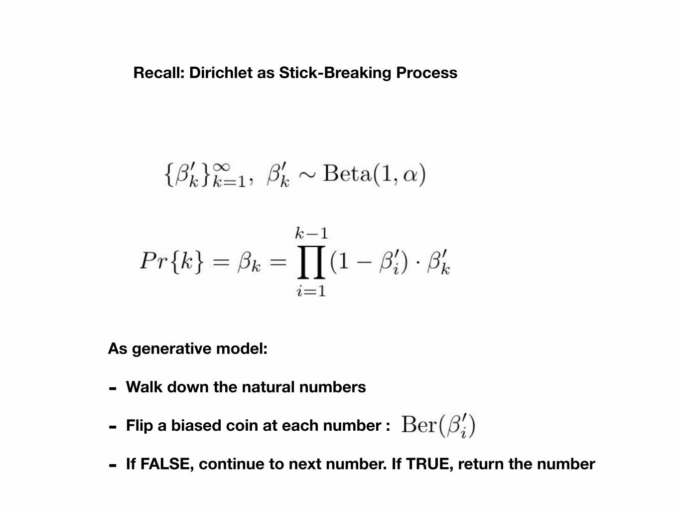
Recall: Dirichlet as Stick-Breaking Process
As generative model:
- Walk down the natural numbers
- Flip a biased coin at each number :
- If FALSE, continue to next number. If TRUE, return the number

As probabilistic program

As probabilistic program

Universal Inference for Probabilistic Programming
Languages

So far…
• Build complicated probabilistic models with PPLs
• Using sample statements: Specify prior generative proc.
• Using factor statements: Specify data likelihood
• A prob. program represents posterior over possible execution “traces”
How to develop generic inference algorithms?

What is a “Trace”?• Sequence of M sample statements
• Sequence of M sampled values
• Sequence of N factor statements
{xj}Mj=1
{fj , ✓j}Mj=1
{gi,�i, yi}Ni=1

Inference over traces• Trace probability:
• Posterior over traces:
• What we care about:
E⇡(x) [f(x)]
Sampling based inference over “traces”
Inference over trace space: exploration—exploitation task
• Explore possible execution paths
• As a side-effect, compute “goodness” of a trace
• Exploit good (more probable) traces
• Return projection of the posterior over traces

Inference over execution traces
x1 ⇠ Categorical(1
3,1
3,1
3)
x2|x1 = 0 ⇠ Poisson(7)
x2|x1 = 2 ⇠ Poisson(9)
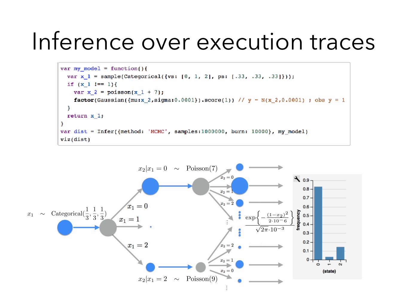
Inference over execution traces
x1 ⇠ Categorical(1
3,1
3,1
3)
x2|x1 = 0 ⇠ Poisson(7)
x2|x1 = 2 ⇠ Poisson(9)
exp
⇢� (1�x2)2
2·10�6
�
p2⇡·10�3
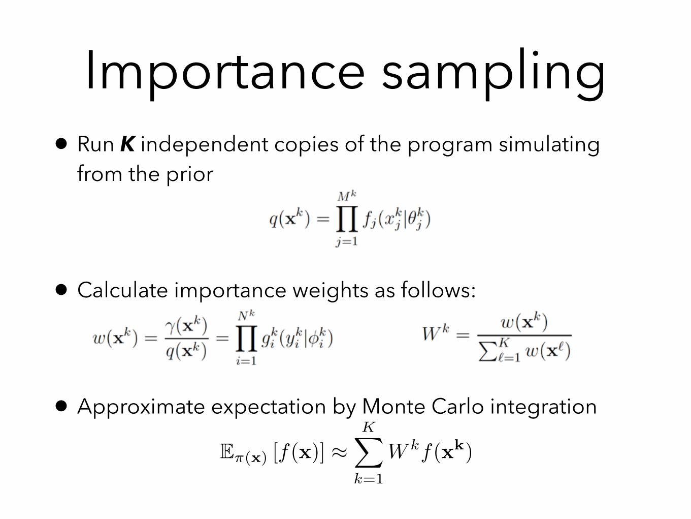
Importance sampling• Run K independent copies of the program simulating
from the prior
• Calculate importance weights as follows:
• Approximate expectation by Monte Carlo integration
E⇡(x) [f(x)] ⇡KX
k=1
W kf(xk)

Importance sampling
f(xK), wK
f(x1), w1
f(x2), w2

Single-Site Metropolis—Hastings
Want samples from
• Pick a proposal distribution that generates a new trace given current trace
• Use Metropolis—Hastings acceptance

Single-Site Metropolis—Hastings
↵1
↵2
↵K

Single-Site Metropolis—Hastings
q(x0|xs) =1
Ms(x0
l|xsl )
M 0Y
j=l+1
f 0j(x
0j |✓0j)
Ms = Number of random elements in old trace
(x0l|xs
l ) = Proposal distribution for the lth random element
Can set

What did we cover?
CHURCH
WebPPL
ANGLICAN
VENTURE
MONAD-BAYES

What did we miss?

That’s all folks!