Probabilistic Robotics

Bayes Filter Implementations

Gaussian filters

•Prediction

•Correction

Bayes Filter Reminder

111 )(),|()( tttttt dxxbelxuxpxbel

)()|()( tttt xbelxzpxbel

Gaussians

2

2)(

2

1

2

2

1)(

:),(~)(

x

exp

Nxp

-

Univariate

)()(2

1

2/12/

1

)2(

1)(

:)(~)(

μxΣμx

Σx

Σμx

t

ep

,Νp

d

Multivariate

),(~),(~ 22

2

abaNYbaXY

NX

Properties of Gaussians

22

21

222

21

21

122

21

22

212222

2111 1

,~)()(),(~

),(~

NXpXpNX

NX

• We stay in the “Gaussian world” as long as we start with Gaussians and perform only linear transformations.

),(~),(~ TAABANY

BAXY

NX

Multivariate Gaussians

12

11

221

11

21

221

222

111 1,~)()(

),(~

),(~

NXpXpNX

NX

6

Discrete Kalman Filter

tttttt uBxAx 1

tttt xCz

Estimates the state x of a discrete-time controlled process that is governed by the linear stochastic difference equation

with a measurement

7

Components of a Kalman Filter

t

Matrix (nxn) that describes how the state evolves from t to t-1 without controls or noise.

tA

Matrix (nxl) that describes how the control ut changes the state from t to t-1.tB

Matrix (kxn) that describes how to map the state xt to an observation zt.tC

t

Random variables representing the process and measurement noise that are assumed to be independent and normally distributed with covariance Rt and Qt respectively.

8

Kalman Filter Updates in 1D

9

Kalman Filter Updates in 1D

1)(with )(

)()(

tTttt

Tttt

tttt

ttttttt QCCCK

CKI

CzKxbel

2,

2

2

22 with )1(

)()(

tobst

tt

ttt

tttttt K

K

zKxbel

10

Kalman Filter Updates in 1D

tTtttt

tttttt RAA

uBAxbel

1

1)(

2

,2221)(

tactttt

tttttt a

ubaxbel

11

Kalman Filter Updates

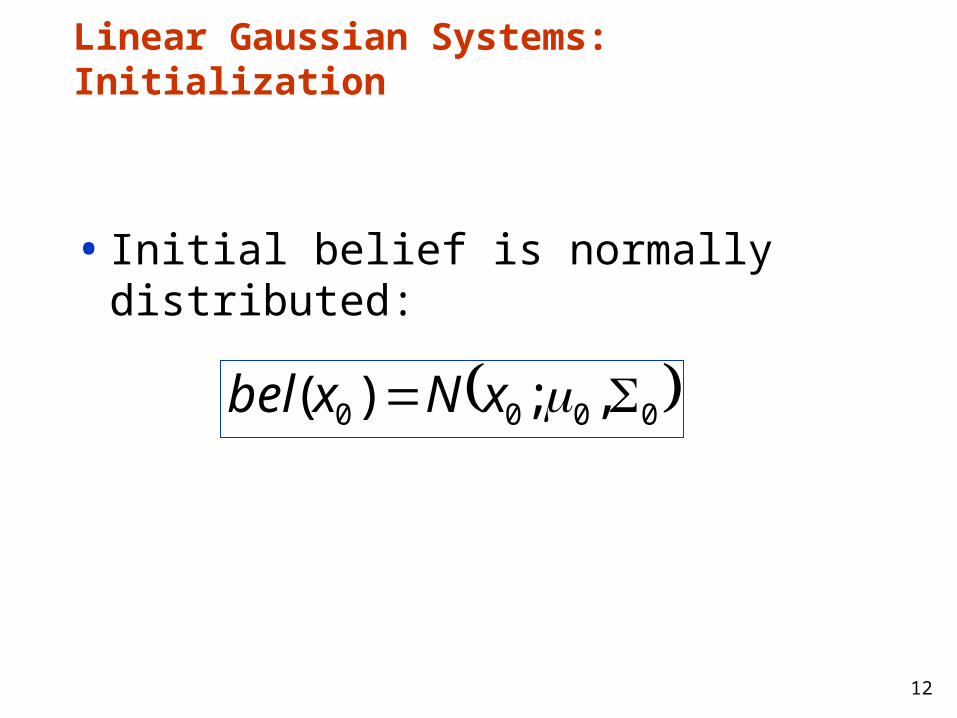
12

0000 ,;)( xNxbel

Linear Gaussian Systems: Initialization

• Initial belief is normally distributed:

13

• Dynamics are linear function of state and control plus additive noise:

tttttt uBxAx 1

Linear Gaussian Systems: Dynamics

ttttttttt RuBxAxNxuxp ,;),|( 11

1111

111

,;~,;~

)(),|()(

ttttttttt

tttttt

xNRuBxAxN

dxxbelxuxpxbel

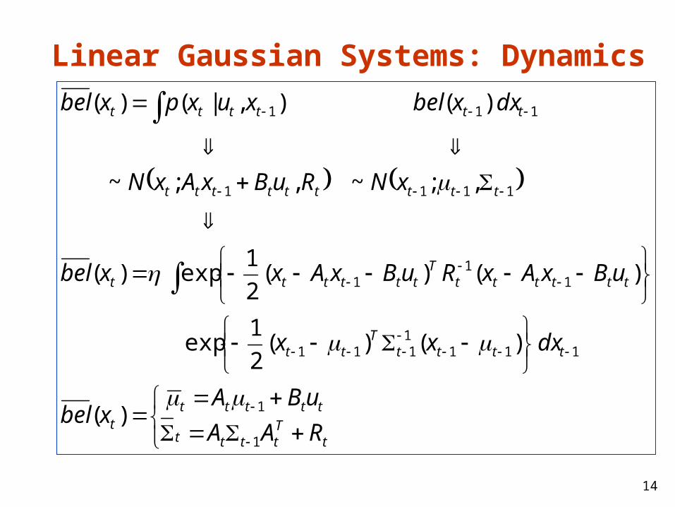
14

Linear Gaussian Systems: Dynamics

tTtttt

tttttt

ttttT

tt

ttttttT

tttttt

ttttttttt

tttttt

RAA

uBAxbel

dxxx

uBxAxRuBxAxxbel

xNRuBxAxN

dxxbelxuxpxbel

1

1

1111111

11

1

1111

111

)(

)()(2

1exp

)()(2

1exp)(

,;~,;~

)(),|()(

15

• Observations are linear function of state plus additive noise:

tttt xCz

Linear Gaussian Systems: Observations

tttttt QxCzNxzp ,;)|(

ttttttt

tttt

xNQxCzN

xbelxzpxbel

,;~,;~

)()|()(

16

Linear Gaussian Systems: Observations

1

11

)(with )(

)()(

)()(2

1exp)()(

2

1exp)(

,;~,;~

)()|()(

tTttt

Tttt

tttt

ttttttt

tttT

ttttttT

tttt

ttttttt

tttt

QCCCKCKI

CzKxbel

xxxCzQxCzxbel

xNQxCzN

xbelxzpxbel

17

Kalman Filter Algorithm

1. Algorithm Kalman_filter( t-1, t-1, ut, zt):

2. Prediction:3. 4.

5. Correction:6. 7. 8.

9. Return t, t

ttttt uBA 1

tTtttt RAA 1

1)( tTttt

Tttt QCCCK

)( tttttt CzK

tttt CKI )(

18

The Prediction-Correction-Cycle

tTtttt

tttttt RAA

uBAxbel

1

1)(

2

,2221)(

tactttt

tttttt a

ubaxbel

Prediction

19

The Prediction-Correction-Cycle

1)(,)(

)()(

tTttt

Tttt

tttt

ttttttt QCCCK

CKI

CzKxbel

2,

2

2

22 ,)1(

)()(

tobst

tt

ttt

tttttt K

K

zKxbel

Correction

20

The Prediction-Correction-Cycle

1)(,)(

)()(

tTttt

Tttt

tttt

ttttttt QCCCK

CKI

CzKxbel

2,

2

2

22 ,)1(

)()(

tobst

tt

ttt

tttttt K

K

zKxbel

tTtttt

tttttt RAA

uBAxbel

1

1)(

2

,2221)(

tactttt

tttttt a

ubaxbel

Correction

Prediction

21

Kalman Filter Summary

•Highly efficient: Polynomial in measurement dimensionality k and state dimensionality n: O(k2.376 + n2)

•Optimal for linear Gaussian systems!

•Most robotics systems are nonlinear!

22

Nonlinear Dynamic Systems

•Most realistic robotic problems involve nonlinear functions

),( 1 ttt xugx

)( tt xhz

23

Linearity Assumption Revisited

24

Non-linear Function

25

EKF Linearization (1)

26

EKF Linearization (2)

27

EKF Linearization (3)

28

EKF Linearization (4)

29

EKF Linearization (5)

30

•Prediction:

•Correction:

EKF Linearization: First Order Taylor Series Expansion

)(),(),(

)(),(

),(),(

1111

111

111

ttttttt

ttt

tttttt

xGugxug

xx

ugugxug

)()()(

)()(

)()(

ttttt

ttt

ttt

xHhxh

xx

hhxh

31

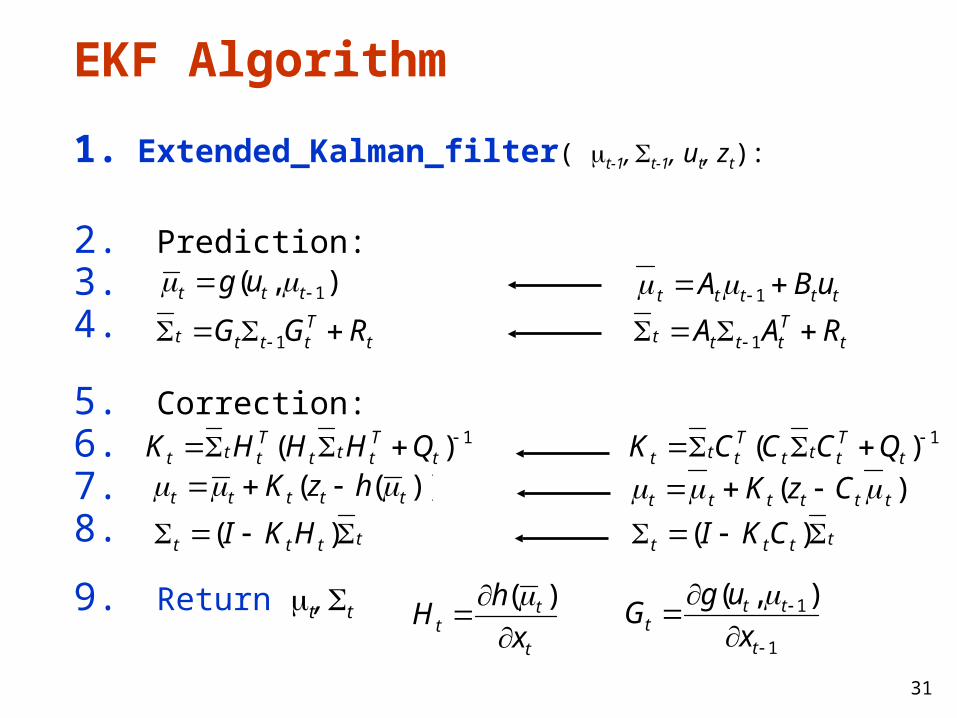
EKF Algorithm

1. Extended_Kalman_filter( t-1, t-1, ut, zt):

2. Prediction:3. 4.

5. Correction:6. 7. 8.

9. Return t, t

),( 1 ttt ug

tTtttt RGG 1

1)( tTttt

Tttt QHHHK

))(( ttttt hzK

tttt HKI )(

1

1),(

t

ttt x

ugG

t

tt x

hH

)(

ttttt uBA 1

tTtttt RAA 1

1)( tTttt

Tttt QCCCK

)( tttttt CzK

tttt CKI )(

32

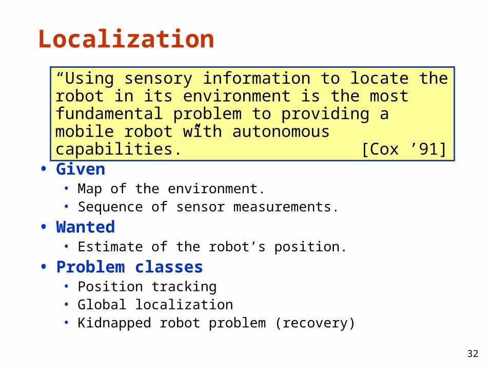
Localization

• Given • Map of the environment.• Sequence of sensor measurements.

• Wanted• Estimate of the robot’s position.

• Problem classes• Position tracking• Global localization• Kidnapped robot problem (recovery)

“Using sensory information to locate the robot in its environment is the most fundamental problem to providing a mobile robot with autonomous capabilities.” [Cox ’91]

33

Landmark-based Localization

34

1. EKF_localization ( t-1, t-1, ut, zt, m):

Prediction:

2.

3.

4.

5.

6.

),( 1 ttt ug Tttt

Ttttt VMVGG 1

,1,1,1

,1,1,1

,1,1,1

1

1

'''

'''

'''

),(

tytxt

tytxt

tytxt

t

ttt

yyy

xxx

x

ugG

tt

tt

tt

t

ttt

v

y

v

y

x

v

x

u

ugV

''

''

''

),( 1

2

43

221

||||0

0||||

tt

ttt

v

vM

Motion noise

Jacobian of g w.r.t location

Predicted mean

Predicted covariance

Jacobian of g w.r.t control

35

1. EKF_localization ( t-1, t-1, ut, zt, m):

Correction:

2.

3.

4.

5.

6.

7.

8.

)ˆ( ttttt zzK

tttt HKI

,

,

,

,

,

,),(

t

t

t

t

yt

t

yt

t

xt

t

xt

t

t

tt

rrr

x

mhH

,,,

2,

2,

,2atanˆ

txtxyty

ytyxtxt

mm

mmz

tTtttt QHHS

1 tTttt SHK

2

2

0

0

r

rtQ

Predicted measurement mean

Pred. measurement covariance

Kalman gain

Updated mean

Updated covariance

Jacobian of h w.r.t location

36

EKF Prediction Step

37

EKF Observation Prediction Step

38

EKF Correction Step

39

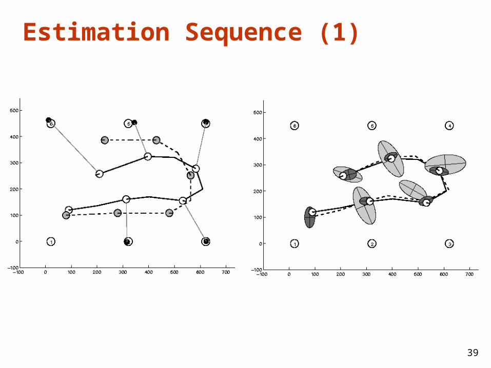
Estimation Sequence (1)

40

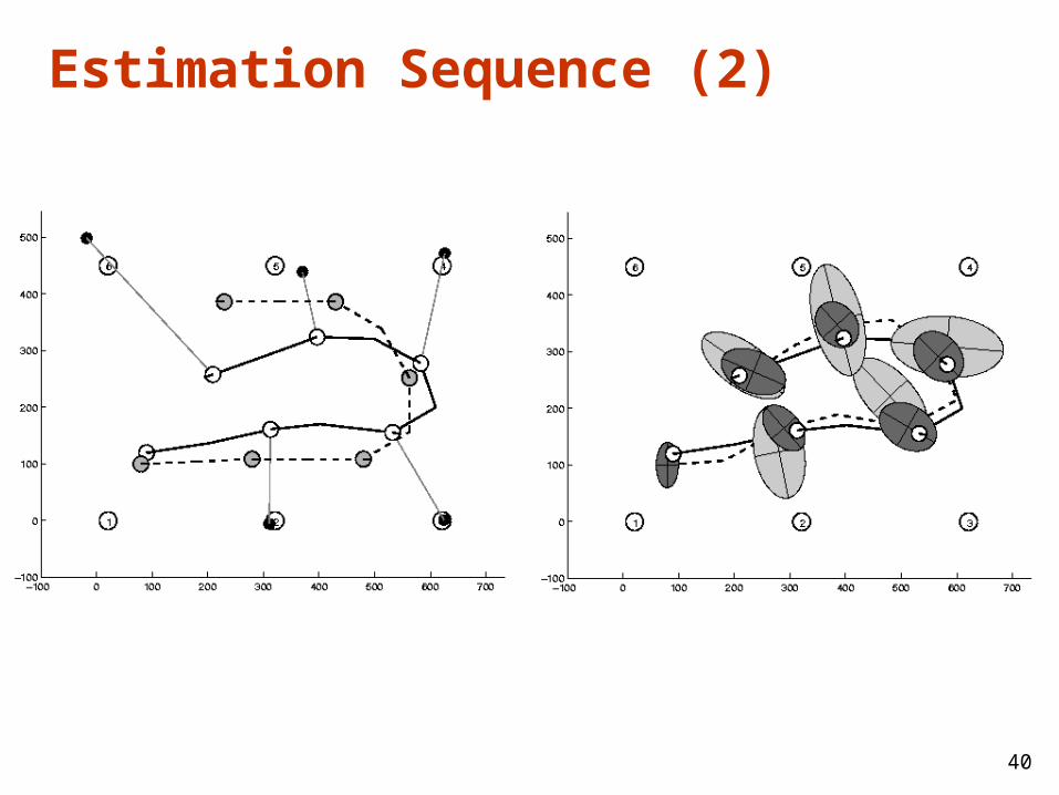
Estimation Sequence (2)

41

Comparison to GroundTruth

42

EKF Summary

•Highly efficient: Polynomial in measurement dimensionality k and state dimensionality n: O(k2.376 + n2)

•Not optimal!•Can diverge if nonlinearities are large!•Works surprisingly well even when all

assumptions are violated!

43

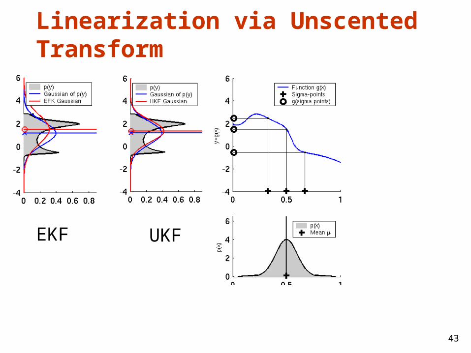
Linearization via Unscented Transform

EKF UKF

44

UKF Sigma-Point Estimate (2)

EKF UKF

45

UKF Sigma-Point Estimate (3)

EKF UKF

46

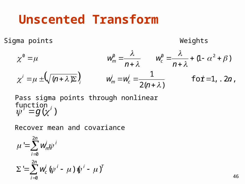
Unscented Transform

nin

wwn

nw

nw

ic

imi

i

cm

2,...,1for )(2

1 )(

)1( 2000

Sigma points Weights

)( ii g

n

i

Tiiic

n

i

iim

w

w

2

0

2

0

))(('

'

Pass sigma points through nonlinear function

Recover mean and covariance

47

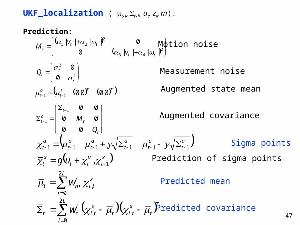
UKF_localization ( t-1, t-1, ut, zt, m):

Prediction:

2

43

221

||||0

0||||

tt

ttt

v

vM

2

2

0

0

r

rtQ

TTTt

at 000011

t

t

tat

Q

M

00

00

001

1

at

at

at

at

at

at 111111

xt

utt

xt ug 1,

L

i

T

txtit

xti

ict w

2

0,,

L

i

xti

imt w

2

0,

Motion noise

Measurement noise

Augmented state mean

Augmented covariance

Sigma points

Prediction of sigma points

Predicted mean

Predicted covariance

48

UKF_localization ( t-1, t-1, ut, zt, m):

Correction:

zt

xtt h

L

iti

imt wz

2

0,ˆ

Measurement sigma points

Predicted measurement mean

Pred. measurement covariance

Cross-covariance

Kalman gain

Updated mean

Updated covariance

Ttti

L

itti

ict zzwS ˆˆ ,

2

0,

Ttti

L

it

xti

ic

zxt zw ˆ,

2

0,

,

1, tzx

tt SK

)ˆ( ttttt zzK

Tttttt KSK

49

1. EKF_localization ( t-1, t-1, ut, zt, m):

Correction:

2.

3.

4.

5.

6.

7.

8.

)ˆ( ttttt zzK

tttt HKI

,

,

,

,

,

,),(

t

t

t

t

yt

t

yt

t

xt

t

xt

t

t

tt

rrr

x

mhH

,,,

2,

2,

,2atanˆ

txtxyty

ytyxtxt

mm

mmz

tTtttt QHHS

1 tTttt SHK

2

2

0

0

r

rtQ

Predicted measurement mean

Pred. measurement covariance

Kalman gain

Updated mean

Updated covariance

Jacobian of h w.r.t location

50

UKF Prediction Step

51

UKF Observation Prediction Step

52

UKF Correction Step

53

EKF Correction Step

54

Estimation Sequence

EKF PF UKF

55

Estimation Sequence

EKF UKF

56

Prediction Quality

EKF UKF

57

UKF Summary

•Highly efficient: Same complexity as EKF, with a constant factor slower in typical practical applications

•Better linearization than EKF: Accurate in first two terms of Taylor expansion (EKF only first term)

•Derivative-free: No Jacobians needed

•Still not optimal!

58

• [Arras et al. 98]:

• Laser range-finder and vision

• High precision (<1cm accuracy)

Kalman Filter-based System

[Courtesy of Kai Arras]

59

Multi-hypothesisTracking

60

• Belief is represented by multiple hypotheses

• Each hypothesis is tracked by a Kalman filter

• Additional problems:

• Data association: Which observation

corresponds to which hypothesis?

• Hypothesis management: When to add / delete

hypotheses?

• Huge body of literature on target tracking, motion

correspondence etc.

Localization With MHT

61

• Hypotheses are extracted from LRF scans

• Each hypothesis has probability of being the correct one:

• Hypothesis probability is computed using Bayes’ rule

• Hypotheses with low probability are deleted.

• New candidates are extracted from LRF scans.

MHT: Implemented System (1)

)}(,,ˆ{ iiii HPxH

},{ jjj RzC

)(

)()|()|(

sP

HPHsPsHP ii

i

[Jensfelt et al. ’00]

62

MHT: Implemented System (2)

Courtesy of P. Jensfelt and S. Kristensen

63

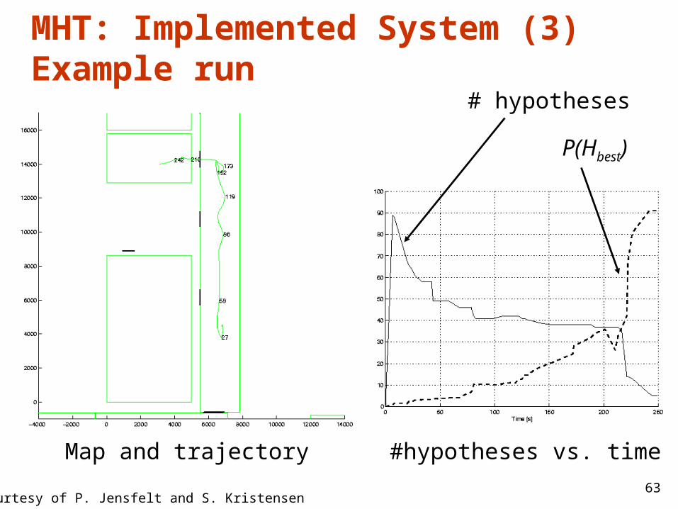
MHT: Implemented System (3)Example run

Map and trajectory

# hypotheses

#hypotheses vs. time

P(Hbest)

Courtesy of P. Jensfelt and S. Kristensen