Probabilistic Robotics

FastSLAM

Sebastian Thrun

(abridged and adapted by Rodrigo Ventura in Oct-2008)

2

  SLAM stands for simultaneous localization and mapping

  The task of building a map while estimating the pose of the robot relative to this map

  Why is SLAM hard? Chicken and egg problem: a map is needed to localize the robot and a pose estimate is needed to build a map

The SLAM Problem

3

Given:   The robot’s

controls

 Observations of nearby features

Estimate:  Map of features

  Path of the robot

The SLAM Problem

A robot moving though an unknown, static environment

4

Why is SLAM a hard problem?

SLAM: robot path and map are both unknown!

Robot path error correlates errors in the map

5

Why is SLAM a hard problem?

  In the real world, the mapping between observations and landmarks is unknown

  Picking wrong data associations can have catastrophic consequences

  Pose error correlates data associations

Robot pose uncertainty

6

Data Association Problem

  A data association is an assignment of observations to landmarks

  In general there are more than (n observations, m landmarks) possible associations

  Also called “assignment problem”

7

  Represent belief by random samples

  Estimation of non-Gaussian, nonlinear processes

  Sampling Importance Resampling (SIR) principle

 Draw the new generation of particles

 Assign an importance weight to each particle

 Resampling

  Typical application scenarios are tracking, localization, …

Particle Filters

8

  A particle filter can be used to solve both problems

  Localization: state space < x, y, θ>

  SLAM: state space < x, y, θ, map>

  for landmark maps = < l1, l2, …, lm>

  for grid maps = < c11, c12, …, c1n, c21, …, cnm>

  Problem: The number of particles needed to represent a posterior grows exponentially with the dimension of the state space!

Localization vs. SLAM

9

  Is there a dependency between the dimensions of the state space?

  If so, can we use the dependency to solve the problem more efficiently?

Dependencies

10

  Is there a dependency between the dimensions of the state space?

  If so, can we use the dependency to solve the problem more efficiently?

  In the SLAM context

 The map depends on the poses of the robot.

 We know how to build a map given the position of the sensor is known.

Dependencies

11

Factored Posterior (Landmarks)

Factorization first introduced by Murphy in 1999

poses map observations & movements

12

Factored Posterior (Landmarks)

SLAM posterior Robot path posterior

landmark positions

Factorization first introduced by Murphy in 1999

Does this help to solve the problem?

poses map observations & movements

13

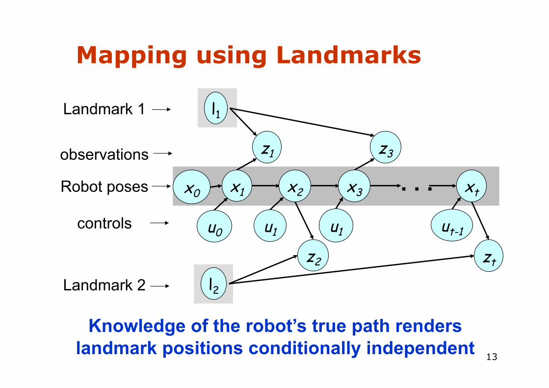
Knowledge of the robot’s true path renders landmark positions conditionally independent

Mapping using Landmarks

. . .

Landmark 1

observations

Robot poses

controls

x1 x2 xt

u1 ut-1

l2

l1

z1

z2

x3

u1

z3

zt

Landmark 2

x0

u0

14

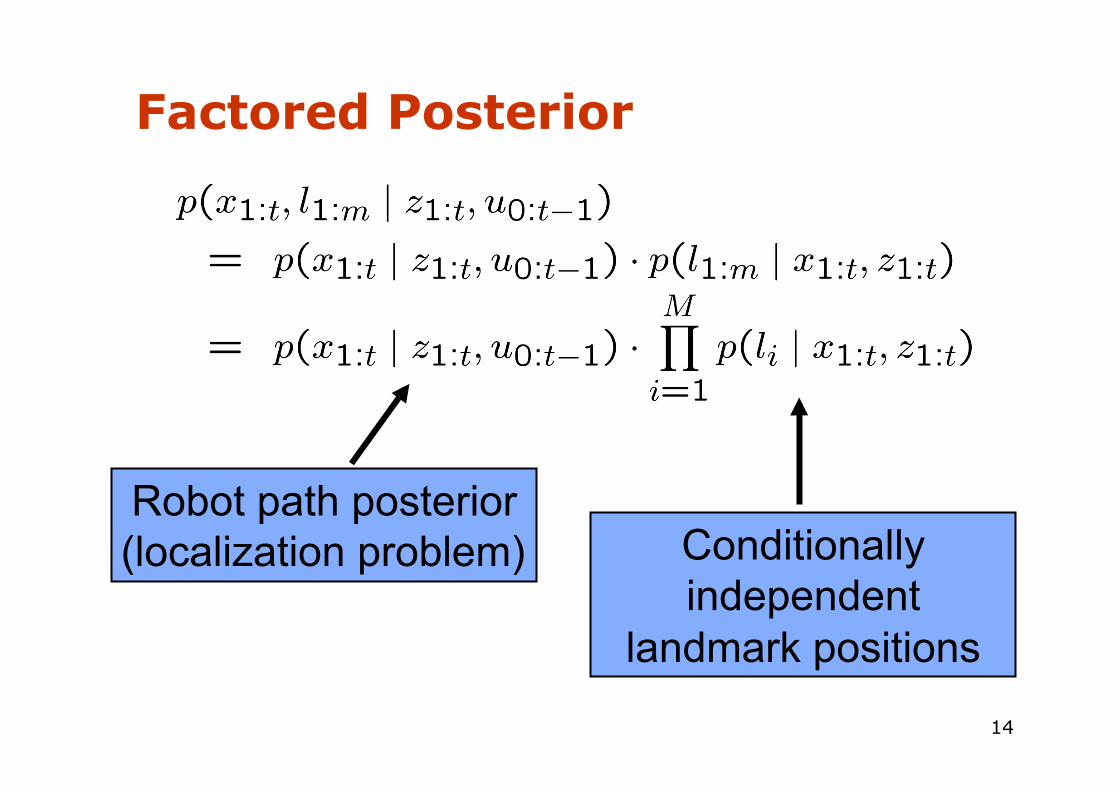
Factored Posterior

Robot path posterior (localization problem) Conditionally

independent landmark positions

15

Rao-Blackwellization

  This factorization is also called Rao-Blackwellization

  Given that the second term can be computed efficiently, particle filtering becomes possible!

16

FastSLAM   Rao-Blackwellized particle filtering based on

landmarks [Montemerlo et al., 2002]

  Each landmark is represented by a 2x2 Extended Kalman Filter (EKF)

  Each particle therefore has to maintain M EKFs

Landmark 1 Landmark 2 Landmark M … x, y, θ

Landmark 1 Landmark 2 Landmark M … x, y, θ Particle #1

Landmark 1 Landmark 2 Landmark M … x, y, θ Particle #2

Particle N

…

17

FastSLAM – Action Update

Particle #1

Particle #2

Particle #3

Landmark #1 Filter

Landmark #2 Filter

18

FastSLAM – Sensor Update

Particle #1

Particle #2

Particle #3

Landmark #1 Filter

Landmark #2 Filter

19

FastSLAM – Sensor Update

Particle #1

Particle #2

Particle #3

Weight = 0.8

Weight = 0.4

Weight = 0.1

20

FastSLAM Complexity

  Update robot particles based on control ut-1

  Incorporate observation zt into Kalman filters

  Resample particle set

N = Number of particles M = Number of map features

O(N) Constant time per particle

O(N•log(M)) Log time per particle

O(N•log(M))

O(N•log(M)) Log time per particle

Log time per particle

21

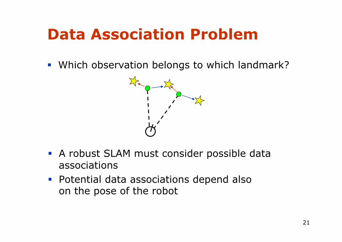
Data Association Problem

  A robust SLAM must consider possible data associations

  Potential data associations depend also on the pose of the robot

  Which observation belongs to which landmark?

22

Multi-Hypothesis Data Association

  Data association is done on a per-particle basis

  Robot pose error is factored out of data association decisions

23

Per-Particle Data Association

Was the observation generated by the red or the blue landmark?

P(observation|red) = 0.3 P(observation|blue) = 0.7

  Two options for per-particle data association   Pick the most probable match   Pick an random association weighted by

the observation likelihoods

  If the probability is too low, generate a new landmark

24

Results – Victoria Park

  4 km traverse   < 5 m RMS

position error   100 particles

Dataset courtesy of University of Sydney

Blue = GPS Yellow = FastSLAM

25

Results – Data Association

26

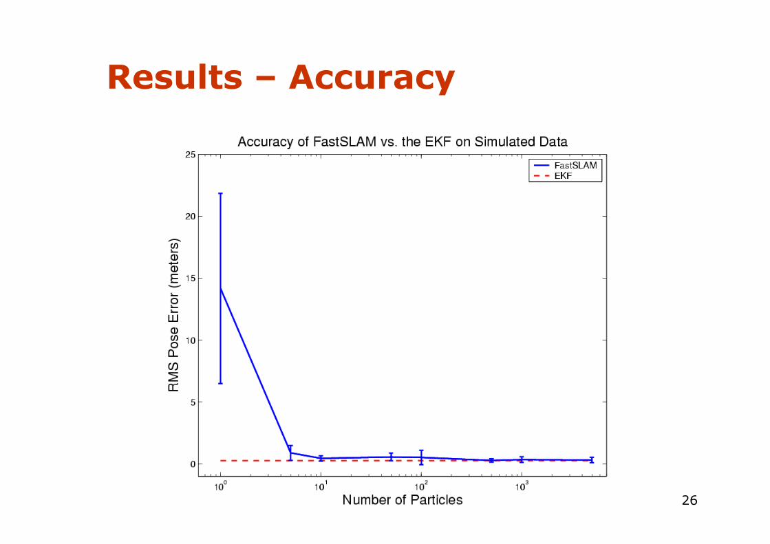
Results – Accuracy

27

  Can we solve the SLAM problem if no pre-defined

landmarks are available?

  Can we use the ideas of FastSLAM to build grid

maps?

  As with landmarks, the map depends on the poses

of the robot during data acquisition

  If the poses are known, grid-based mapping is easy

(“mapping with known poses”)

Grid-based SLAM

28

Rao-Blackwellization

Factorization first introduced by Murphy in 1999

poses map observations & movements

29

Rao-Blackwellization

SLAM posterior

Robot path posterior

Mapping with known poses

Factorization first introduced by Murphy in 1999

poses map observations & movements

30

Rao-Blackwellization

This is localization, use MCL

Use the pose estimate from the MCL part and apply mapping with known poses

31

A Graphical Model of Rao-Blackwellized Mapping

m

x

z

u

x

z

u

2

2

x

z

u

... t

t

x 1

1

0

1 0 t-1

32

Rao-Blackwellized Mapping

  Each particle represents a possible trajectory of the robot

  Each particle   maintains its own map and   updates it upon “mapping with known poses”

  Each particle survives with a probability proportional to the likelihood of the observations relative to its own map

33

Particle Filter Example

map of particle 1 map of particle 3

map of particle 2

3 particles

34

Problem

  Each map is quite big in case of grid maps   Since each particle maintains its own map   Therefore, one needs to keep the number

of particles small

  Solution: Compute better proposal distributions!

  Idea: Improve the pose estimate before applying the particle filter

35

Pose Correction Using Scan Matching

Maximize the likelihood of the i-th pose and map relative to the (i-1)-th pose and map

robot motion current measurement

map constructed so far

36

Motion Model for Scan Matching

Raw Odometry Scan Matching

37

FastSLAM with Improved Odometry

  Scan-matching provides a locally consistent pose correction

  Pre-correct short odometry sequences using scan-matching and use them as input to FastSLAM

  Fewer particles are needed, since the error in the input in smaller

[Haehnel et al., 2003]

38

Further Improvements

  Improved proposals will lead to more accurate maps

  They can be achieved by adapting the proposal distribution according to the most recent observations

  Flexible re-sampling steps can further improve the accuracy.

39

Improved Proposal

  The proposal adapts to the structure of the environment

40

Selective Re-sampling

  Re-sampling is dangerous, since important samples might get lost (particle depletion problem)

  In case of suboptimal proposal distributions re-sampling is necessary to achieve convergence.

  Key question: When should we re-sample?

41

Number of Effective Particles

  Empirical measure of how well the goal distribution is approximated by samples drawn from the proposal

  neff describes “the variance of the particle weights”

  neff is maximal for equal weights. In this case, the distribution is close to the proposal

42

Resampling with Neff

  Only re-sample when neff drops below a given threshold (n/2)

  See [Doucet, ’98; Arulampalam, ’01]

43

Typical Evolution of neff

visiting new areas closing the

first loop

second loop closure

visiting known areas

44

Conclusion

  The ideas of FastSLAM can also be applied in the context of grid maps

  Utilizing accurate sensor observation leads to good proposals and highly efficient filters

  It is similar to scan-matching on a per-particle base

  The number of necessary particles and re-sampling steps can seriously be reduced

  Improved versions of grid-based FastSLAM can handle larger environments than naïve implementations in “real time” since they need one order of magnitude fewer samples

45

More Details on FastSLAM

  M. Montemerlo, S. Thrun, D. Koller, and B. Wegbreit. FastSLAM: A factored solution to simultaneous localization and mapping, AAAI02

  D. Haehnel, W. Burgard, D. Fox, and S. Thrun. An efficient FastSLAM algorithm for generating maps of large-scale cyclic environments from raw laser range measurements, IROS03

  M. Montemerlo, S. Thrun, D. Koller, B. Wegbreit. FastSLAM 2.0: An Improved particle filtering algorithm for simultaneous localization and mapping that provably converges. IJCAI-2003

  G. Grisetti, C. Stachniss, and W. Burgard. Improving grid-based slam with rao-blackwellized particle filters by adaptive proposals and selective resampling, ICRA05

  A. Eliazar and R. Parr. DP-SLAM: Fast, robust simultanous localization and mapping without predetermined landmarks, IJCAI03