probabilistic short-term financial planning

Probabilistic Short-Term Financial PlanningAuthor(s): James L. Pappas and George P. HuberSource: Financial Management, Vol. 2, No. 3 (Autumn, 1973), pp. 36-44Published by: Wiley on behalf of the Financial Management Association InternationalStable URL: http://www.jstor.org/stable/3664985 .

Accessed: 13/06/2014 00:23

Your use of the JSTOR archive indicates your acceptance of the Terms & Conditions of Use, available at .http://www.jstor.org/page/info/about/policies/terms.jsp

.JSTOR is a not-for-profit service that helps scholars, researchers, and students discover, use, and build upon a wide range ofcontent in a trusted digital archive. We use information technology and tools to increase productivity and facilitate new formsof scholarship. For more information about JSTOR, please contact [email protected].

.

Wiley and Financial Management Association International are collaborating with JSTOR to digitize, preserveand extend access to Financial Management.

http://www.jstor.org

This content downloaded from 62.122.72.154 on Fri, 13 Jun 2014 00:23:44 AMAll use subject to JSTOR Terms and Conditions

http://www.jstor.org/action/showPublisher?publisherCode=black

http://www.jstor.org/action/showPublisher?publisherCode=fma

http://www.jstor.org/stable/3664985?origin=JSTOR-pdf

http://www.jstor.org/page/info/about/policies/terms.jsp


PROBABILISTIC SHORT-TERM FINANCIAL PLANNING

JAMES L. PAPPAS and GEORGE P. HUBER

James L. Pappas is Associate Professor of Business in the Graduate School of Business of the University of Wisconsin-Madison. He received his PhD in Finance from UCLA. Professor Pappas has published articles on determination of cost of capital, valuation, and economic analysis of regulated industries; and he is co-author of a recently published textbook, Managerial Economics, Dryden Press, 1972. George P. Huber is Professor of Business in the Graduate School of Business at the University of Wisconsin-Madison and he holds appointments in the Department of Industrial Engineering and the Industrial Relations Research Institute. Professor Huber received his PhD from Purdue University.

C ompanies typically arrange lines of credit or more formal credit agreements with banks primarily to assure availability of funds on short notice. The need for such funds may stem from seasonal fluctua- tions in working capital requirements, from a contin- uing need for additional permanent capital coupled with the desire to seek funds in the capital market at less frequent intervals than would be necessary without bank credit, from a relatively unstable relationship between cash inflows and disbursements, or from a number of other such factors.

The financial manager is responsible for mini- mizing the cost of the funds obtained subject to the requirement that a credit agreement provides the amount of liquidity needed. Thus, he must examine all factors that can influence cost associated with all the credit sources available. This evaluation is not

aimed solely at selecting the least-cost credit arrangement. For example, funds obtained by means of an informal line of credit may well cost less than a similar amount acquired through a contractual agreement. However, with an informal line of credit the firm risks the loss of funds in times of a credit crunch, since such agreements typically do not con- tractually obl'gate the bank. Moreover, under line of credit agreements the interest rate is typically not final until the time of borrowing. With the formal credit agreement, on the other hand, the bank is legally obliga'ed to supply the funds, and the interest rate charged is frequently specified. Thus, the two forms of credit arrangement are dissimilar in significant ways. Hence, they cannot be evaluated as alternatives only on the basis of expected cost. Rather, their comparison is a form of cost-benefit analysis.

Financial Management 36



The Cost of Credit

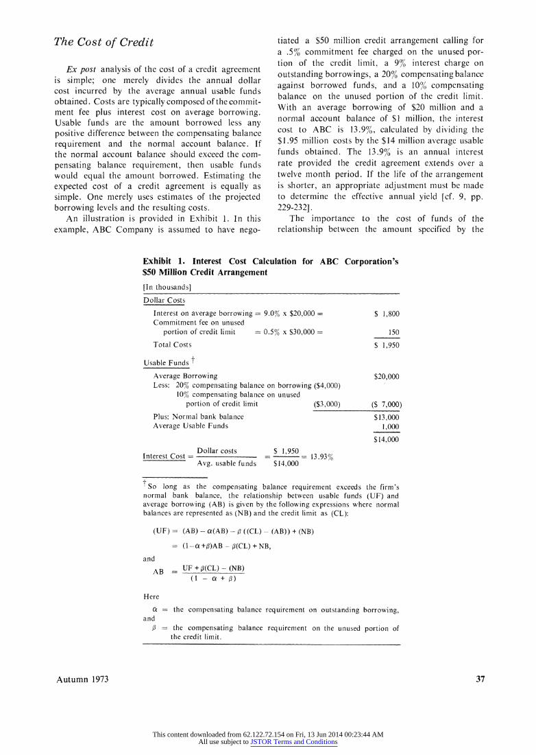
Ex post analysis of the cost of a credit agreement is simple; one merely divides the annual dollar cost incurred by the average annual usable funds obtained. Costs are typically composed of the commitment fee plus interest cost on average borrowing. Usable funds are the amount borrowed less any positive difference between the compensating balance requirement and the normal account balance. If the normal account balance should exceed the compensating balance requirement, then usable funds would equal the amount borrowed. Estimating the expected cost of a credit agreement is equally as simple. One merely uses estimates of the projected borrowing levels and the resulting costs.

An illustration is provided in Exhibit 1. In this example, ABC Company is assumed to have nego-

tiated a $50 million credit arrangement calling for a .5% commitment fee charged on the unused portion of the credit limit, a 9% interest charge on outstanding borrowings, a 20% compensating balance against borrowed funds, and a 10% compensating balance on the unused portion of the credit limit. With an average borrowing of $20 million and a normal account balance of $1 million, the interest cost to ABC is 13.9%, calculated by dividing the $1.95 million costs by the $14 million average usable funds obtained. The 13.9% is an annual interest rate provided the credit agreement extends over a twelve month period. If the life of the arrangement is shorter, an appropriate adjustment must be made to determine the effective annual yield [cf. 9, pp. 229-232].

The importance to the cost of funds of the relationship between the amount specified by the

Exhibit 1. Interest Cost Calculation for ABC Corporation's $50 Million Credit Arrangement

[In thousands]

Dollar Costs

Interest on average borrowing = 9.0% x $20,000 = Commitment fee on unused

portion of credit limit = 0.5% x $30,000 =

Total Costs

Usable Funds t

Average Borrowing Less: 20% compensating balance on borrowing ($4,000)

10% compensating balance on unused portion of credit limit ($3,000)

Plus: Normal bank balance Average Usable Funds

Dollar costs Interest Cost =

Avg. usable funds

$13,000 1,000

$14,000

$ 1,950 = 13.93% $14,000

tSo long as the compensating balance requirement exceeds the firm's normal bank balance, the relationship between usable funds (UF) and average borrowing (AB) is given by the following expressions where normal balances are represented as (NB) and the credit limit as (CL):

(UF) = (AB) - a(AB) - , ((CL) - (AB)) + (NB)

= (1-a+3)AB - (CL) + NB,

and

AB = UF+P(CL)-(NB) (1 - a+ )

Here

o = the compensating balance requirement on outstanding borrowing, and

P = the compensating balance requirement on the unused portion of the credit limit.

Autumn 1973

$ 1,800

150

$ 1,950

$20,000

($ 7,000)

37



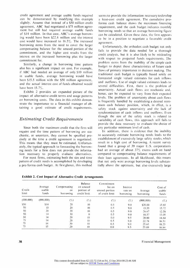
credit agreement and average usable funds required can be demonstrated by modifying this example slightly. Assume that instead of a $50 million credit agreement, ABC had negotiated a $75 million agreement but still had required average usable funds of $14 million. In that case, ABC's average borrowing would have been $22.8 million and the interest cost would have increased to 16.5%. The increased borrowing stems from the need to cover the larger compensating balance for the unused portion of the commitment, and the higher cost results from the interest on the increased borrowing plus the larger commitment fee.

Similarly, a change in borrowing time pattern also has a significant impact on cost. For example, if ABC had needed an average of only $10 million in usable funds, average borrowing would have been $15.5 million with the $50 million agreement, and the actual interest cost of funds obtained would have been 15.7%.

Exhibit 2 provides an expanded picture of the impact of alternative credit terms and usage patterns on borrowing costs. The data in this exhibit demonstrate the importance to a financial manager of ob- taining a good estimate of credit requirements.

Estimating Credit Requirements

Since both the maximum credit that the firm will require and the time pattern of borrowing are stochastic, or uncertain, they cannot be specified precisely at the time a credit agreement is negotiated. This means that they must be estimated. Unfortun- ately, the typical approach to forecasting the borrowing needs for a firm does not provide the information necessary to properly evaluate alternatives.

For most firms, estimating both the size and time pattern of credit needs is accomplished by developing a pro forma cash budget. At first glance, this method

seems to provide the information necessary to develop a least-cost credit agreement. The cumulative pro- forma cash balance shows the maximum financing requirement, and the cash budget indicates monthly borrowing needs so that an average borrowing figure can be calculated. Given these data, the firm appears to be in a position to negotiate a favorable credit agreement.

Unfortunately, the orthodox cash budget not only fails to provide the data needed for a thorough credit analysis, but it is also likely to be misleading with respect to projected funds requirements. The problem stems from the inability of the simple cash budget to depict those characteristics of future cash flows of primary importance in decision making. The traditional cash budget is typically based solely on forecasted single valued estimates for cash inflows and outflows. Use of single valued estimates leads to several difficulties. First, there is the problem of uncertainty. Actual cash flows are stochastic and, hence, can be expected to vary from their expected levels. The problem of uncertainty about cash flows is frequently handled by establishing a desired minimum cash balance position, which, in effect, is a safety stock against uncertainty and the lack of synchronization of cash inflows and outflows. Even though the size of the safety stock is related to variability of cash flows, this approach still fails to provide the data necessary to evaluate the choice of any particular minimum level of cash.

In addition, there is evidence that the inability to accurately estimate borrowing needs leads to the establishment of excessively large safety stocks, which result in a high cost of borrowing. A recent survey found that a group of 39 major U.S. corporations had an average of about 37% excess cash on hand compared to compensating balance requirements of their loan agreements. In all likelihood, this means that not only were average borrowing levels substan- tially above the optimum, but also excessively large

Exhibit 2. Cost Impact of Alternative Credit Arrangements

Balance Commitment Average Compensating on unused fee on Interest Cost of

Credit usable on portion of unused portion rate on Average usable limit funds borrowing credit limit of credit limit borrowing borrowing funds

(000,000) (000,000) (%) ()(%) (000,000) (%) $50 $14 20 10 0.5 9.0 $20.00 13.93

50 10 20 10 0.5 9.0 15.55 15.72 50 20 20 10 0.5 9.0 26.67 12.58 50 14 30 0 0.5 9.0 18.57 13.05 50 14 20 10 0.0 9.5 20.00 14.64 75 14 20 10 0.5 9.0 22.78 16.51 75 14 30 10 0.5 9.0 25.63 18.23 75 15 20 10 0.0 9.5 23.89 16.84




loan agreements had been negotiated. Another recently reported example [1] showed a large Mid- western firm paying 28% for its bank credit for precisely these reasons.

A second problem arising from the cash budget approach to financial planning lies in the estimation of cumulative borrowing needs. This approach does not reveal intra- and inter-period cash flow relation- ships, and these influence the pattern of cumulative net cash flows. For example, activities associated with greater than expected cash inflows may also require greater than expected expenses or outflows. Similarly, if sales and revenues fall below expectations, it is likely that cash outflows will also be lower than their expected value. Such a situation is reflected by a significant intra-period correlation of cash flows.

In addition, it is reasonable to expect important inter-period cash flow correlations. If, for example, sales exceed expectations in one period, it is frequently the case that they will also be higher than initially expected in the following period. Similarly, if a firm experiences higher than expected costs in its production system, the factors that led to the added costs may well cause a similar pattern in succeeding periods. Given either intra- or inter-period correlations of cash flows, the simple cash budget procedure for projecting financial requirements will

provide misleading data.

A Simulation Approach to Estimating Cash Needs

Fortunately, a rather simple extension of cash budgeting methodology provides the information necessary to correctly analyze alternative credit possibilities. The extension involves the use of a simulation model. Such a model provides more accurate answers than can a simple cash budget to such questions as: What is the maximum amount of credit that the firm is likely to require? What is the expected average borrowing figure? Additionally, the simulation approach provides other much needed information by answering questions like: What is the probability that the maximum borrowing requirement will exceed any given dollar amount? What are the probabilities associated with positive loan balances in any given month? What is the probability that the firm will be able to repay all borrowing by the end of the planning period?

Overall, simulating cash flows should provide a positive economic benefit, but it does require more extensive data than the usual cash budget approach. Instead of identifying simply the expected value for each monthly inflow and outflow, simulation requires that we estimate the probabilities of other possible

flows, as well as intra- and inter-period cash flow correlation coefficients. While this may appear for- midable, we will demonstrate that whatever source of information is used for developing point forecasts of expenditures and receipts is usually sufficient for developing distribution forecasts.

Developing Distribution Forecasts from Historical Data

It may be that we have accurate data of our historical expenditures and receipts and believe that their future values will be a straight-forward extra- polation of their past values. If this is the case, then we should compute the probability distributions for future time periods as follows.

1. Using either trend analysis or a seasonal model, construct a forecasting model that would have accurately predicted the recent history of the firm's cash flows (expenditures and receipts). (The reader is referred to the Nelson text [4] for an excellent exposition on this process.)

2. Use the model to develop an estimate of the expected cash flow, Yt, in each period covered by the data, and subtract the actual cash flow, Yt, from the expected cash flow to compute the forecast error, et= Yt-Yt, for each time period, t. Draw a histogram or probability distribution of these errors. It has a mean of zero.

3. Modify this parent distribution for use at each point t, to account for the fact that the forecast, Yt, of any point that is far removed from the center of the historical data will be less accurate than the forecast of a point closer to the mean, t, of the time periods examined. Since the points we are forecasting are outside the range of the historical data, their probability distributions will have greater variance than the average variance calculated in the forecasting model. We can adjust for this by multiplying each of the errors shown in the histogram developed in step 2 by an adjustment factor, 5t, for each future period we plan to incorporate into our analysis, while retaining the original probability for each. The term 6t, which is to unity as the standard deviation for any Y* is to the standard

:gc t deviation of Yt at t, is algebraically correct for least squares forecasts and is offered here as a heuristic for other forecasts [cf. 5]. The equation for 6t is:

6t= 1 +t + -2 (1)

I 1 N 2 (t-t)2

t=l

Autumn 1973 39



where N is the number of data points used to obtain the least squares trend line or the parameters of a seasonal model. This adjustment procedure has the effect of appropriately increasing the variance of the estimate, Yt, for each forecast

period, t. As can be seen from inspection of the formula for bt or from the forthcoming example calculation, only if N is quite small or t is much larger than t, is bt significantly different from unity.

4. Use the model to forecast the expected cash flow for each of future time periods important to the bank credit arrangement.

5. Estimate the probability distribution for each of the future time periods by adding the mean of the distribution (computed in step 4) to the values of the probability distribution of historical errors, computed in step 3, i.e., shift the probability distribution from a mean of zero to a mean estimated by the forecasting model.

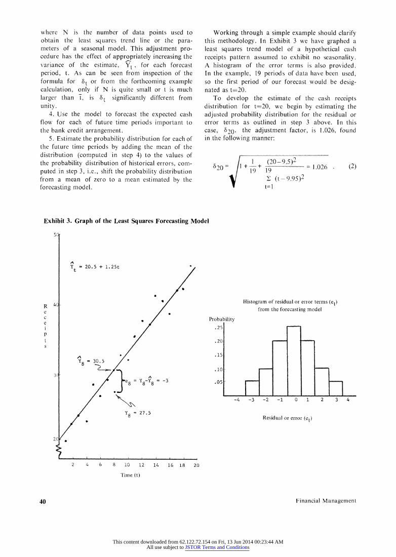
Working through a simple example should clarify this methodology. In Exhibit 3 we have graphed a least squares trend model of a hypothetical cash receipts pattern assumed to exhibit no seasonality. A histogram of the error terms is also provided. In the example, 19 periods of data have been used, so the first period of our forecast would be desig- nated as t=20.

To develop the estimate of the cash receipts distribution for t=20, we begin by estimating the adjusted probability distribution for the residual or error terms as outlined in step 3 above. In this case, 820, the adjustment factor, is 1.026, found in the following manner:

(20-9.5)2 19^ = 1.026 19

2 (t- 9.95)2 t= I

(2)

Exhibit 3. Graph of the Least Squares Forecasting Model

Y = 20.5 + 1.25t t

Y a 30.5 / D/

-- ''''' ,''''''''''''_'''

A

e8 = y -Y8 = -3

Y8 = 27.5

Histogram of residual or error terms (et) from the forecasting model

Probability .25

.20

.15

.10

.05-

-4 -3 -2 -1 0 1 2 7

3 4

Residual or error (et)

2 4 6 8 10 12 14 16 18

Time (t)

Financial Management

R e c e i p S s

20

I

40

620 = + - + 19

!



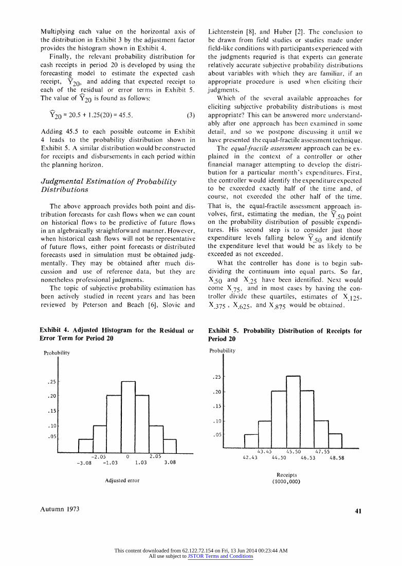
Multiplying each value on the horizontal axis of the distribution in Exhibit 3 by the adjustment factor provides the histogram shown in Exhibit 4.

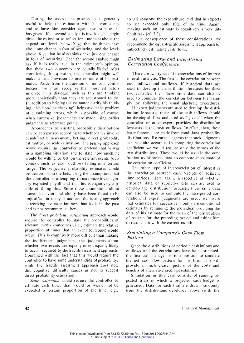
Finally, the relevant probability distribution for cash receipts in period 20 is developed by using the forecasting model to estimate the expected cash receipt, Y20, and adding that expected receipt to each of the residual or error terms in Exhibit 5. The value of Y20 is found as follows:

Y20 = 20.5 + 1.25(20)= 45.5. (3)

Adding 45.5 to each possible outcome in Exhibit 4 leads to the probability distribution shown in Exhibit 5. A similar distribution would be constructed for receipts and disbursements in each period within the planning horizon.

Judgmental Estimation of Probability Distributions

The above approach provides both point and distribution forecasts for cash flows when we can count on historical flows to be predictive of future flows in an algebraically straightforward manner. However, when historical cash flows will not be representative of future flows, either point forecasts or distributed forecasts used in simulation must be obtained judg- mentally. They may be obtained after much dis- cussion and use of reference data, but they are nonetheless professional judgments.

The topic of subjective probability estimation has been actively studied in recent years and has been reviewed by Peterson and Beach [6], Slovic and

Exhibit 4. Adjusted Histogram for the Residual or Error Term for Period 20

Lichtenstein [8], and Huber [2]. The conclusion to be drawn from field studies or studies made under field-like conditions with participants experienced with the judgments requried is that experts can generate relatively accurate subjective probability distributions about variables with which they are familiar, if an appropriate procedure is used when eliciting their judgments.

Which of the several available approaches for eliciting subjective probability distributions is most appropriate? This can be answered more understand- ably after one approach has been examined in some detail, and so we postpone discussing it until we have presented the equal-fractile assessment technique.

The equal-fractile assessment approach can be ex- plained in the context of a controller or other financial manager attempting to develop the distribution for a particular month's expenditures. First, the controller would identify the expenditure expected to be exceeded exactly half of the time and, of course, not exceeded the other half of the time. That is, the equal-fractile assessment approach involves, first, estimating the median, the Y.50 point on the probability distribution of possible expenditures. His second step is to consider just those expenditure levels falling below Y.50 and identify the expenditure level that would be as likely to be exceeded as not exceeded.

What the controller has done is to begin sub- dividing the continuum into equal parts. So far, X50 and X.25 have been identified. Next would come X75, and in most cases by having the controller divide these quartiles, estimates of X125, X.375, X.625, and X.875 would be obtained.

Exhibit 5. Period 20

Probability Distribution of Receipts for

Probability

.25

.20

.15 -

.10

.05

-2.05 -3.08 -1.03

Probability

.25

.20 -

.15

.101

.05

0 2.05 1.03 3.08

43.45 45.50 47.55 42.43 44.50 46.53 48.58

Receipts ($000,000) Adjusted error

Autumn 1973

q v a I I

41



During the assessment process, it is generally useful to help the estimator with his consistency and to have him consider again the estimates he has given. If a second analyst is involved, he might direct the estimator to reflect for a moment about the expenditure levels below X 25 that he thinks have about one chance in four of occurring, and the levels above X.75 that he also thinks have just one chance in four of occurring. Then the second analyst might ask if it is really true, in the estimator's opinion, that these two outcomes are equally likely? After considering this question, the controller might well make a small revision to one or more of his estimates. Aside from the question of minor inconsis- tencies, we must recognize that most estimators involved in a dialogue such as this are thinking more analytically than they are accustomed to do. In addition to helping the estimator clarify his thinking, this "on-line checking" helps avoid the problem of cumulating errors, which is possible, of course, when successive judgements are made using earlier judgments as reference points.

Approaches to eliciting probability distributions can be categorized according to whether they involve equal-fractile assessment, betting, direct probability estimation, or scale estimation. The betting approach would require the controller to pretend that he was in a gambling situation and to state how much he would be willing to bet on the relevant events (outcomes), such as cash outflows falling in a certain range. The subjective probability estimates would be derived from the bets, using the assumptions that the controller is attempting to maximize his imagin- ary expected payoff and that his is cognitively cap- able of doing this. Since these assumptions about human behavior and ability have been found to be unjustified in many situations, the betting approach is receiving less attention now than it did in the past and is not recommended here.

The direct probability estimation approach would require the controller to state the probabilities of relevant events (outcomes), i.e., estimate the relative proportion of times that an event (outcome) would occur. This is cognitively more difficult than making the indifference judgments, the judgments about whether two events are equally or not equally likely to occur, required by the fractile assessment approach. Combined with the fact that this would require the controller to have some understanding of probability, while the fractile assessment approach does not, this cognitive difficulty causes us not to suggest direct probability estimation.

Scale estimation would require the controller to estimate cash flows that would or would not be exceeded a certain proportion of the time, e.g.,

to tell someone the expenditure level that he expects to see exceeded only 10% of the time. Again, making such an estimate is cognitively a very difficult task [cf. 7,3].

As a consequence of these considerations, we recommend the equal-fractile assessment approach for subjectively estimating cash flows.

Estimating Intra- and Inter-Period Correlation Coefficients

There are two types of intercorrelations of interest in credit analysis. The first is the correlation between cash inflows and outflows. If historical data are used to develop the distribution forecasts for these two variables, then these same data can also be used to compute the correlation between them simply by following the usual algebraic procedures.

If expert judgments are used to develop the distribution forecasts, those of the cash inflows should be developed first and used as "givens" when the controller or other expert provides the distribution forecasts of the cash outflows. In effect, then, these latter forecasts are made from conditional probability distributions. Research suggests that such judgments can be quite accurate. In computing the correlation coefficient we would require only the means of the two distributions. These would be used in the same fashion as historical data to compute an estimate of the correlation coefficient.

The other type of intercorrelation of interest is the correlation between cash receipts of adjacent time periods. Here again, irrespective of whether historical data or subjective estimates are used to develop the distribution forecasts, these same data can also be used to compute the inter-period correlation. If expert judgments are used, we insure that estimates for successive months are conditional estimates by reminding the individual providing the data of his estimate for the mean of the distribution of receipts for the preceding period and asking him to reconcile it with the current month.

Simulating a Company's Cash Flow Pattern

Once the distributions of periodic cash inflows and outflows and the correlations have been estimated, the financial manager is in a position to simulate the net cash flow pattern for his firm. This will provide a much clearer picture of the costs and benefits of alternative credit possibilities.

Simulation in this case consists of running re- peated trials in which a projected cash budget is generated. Data for each trial are drawn randomly from the distributions developed above (with the




proper inter- and intra-period correlations), and the resulting cash flow patterns themselves are formed into frequency distributions.

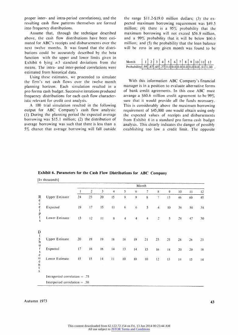
Assume that, through the technique described above, the cash flow distributions have been estimated for ABC's receipts and disbursements over the next twelve months. It was found that the distributions could be accurately described by the beta function with the upper and lower limits given in Exhibit 6 lying +3 standard deviations from the means. The intra- and inter-period correlations were estimated from historical data.

Using these estimates, we proceeded to simulate the firm's net cash flows over the twelve month planning horizon. Each simulation resulted in a pro forma cash budget. Successive iterations produced frequency distributions for each cash flow character- istic relevant for credit cost analysis.

A 100 trial simulation resulted in the following output for ABC Company's cash flow analysis: (1) During the planning period the expected average borrowing was $15.1 million; (2) the distribution of average borrowing was such that there is less than a 5% chance that average borrowing will fall outside

the range $11.2-$19.0 million dollars; (3) the expected maximum borrowing requirement was $49.5 million; (4) there is a 95% probability that the maximum borrowing will not exceed $56.9 million, and a 99% probability that it will be below $60.6 million; and (5) the probability that the loan balance will be zero in any given month was found to be

Month 1 2 3 4 5 6 7 8 9 10 11 12

Probability .95 .87 .65 .27 0.0 0.0 0.0 0.0 0.0 0.0 .51 1.00

With this information ABC Company's financial manager is in a position to evaluate alternative forms of bank credit agreements. In this case ABC must arrange a $60.6 million credit agreement to be 99% sure that it would provide all the funds necessary. This is considerably above the maximum borrowing requirement of $45,000 one would obtain using only the expected values of receipts and disbursements from Exhibit 6 in a standard pro forma cash budget analysis. This clearly indicates the danger of possibly establishing too low a credit limit. The opposite

Exhibit 6. Parameters for the Cash Flow Distributions for ABC Company

[In thousands]

Month

Upper Estimate

Expected

Lower Estimate

Upper Estimate

Expected

Lower Estimate

1 2 3 4 5 6 7 8 9 10 11 12

24 23 20 15 9 9 8 7 13 46 60 45

19 17 15 11 6 6 5 4 10 38 50 38

13 12 11 8 4 4 4 2 5 28 47 30

20 19 19 18 18 19 21 23 25 28 26 23

17 16 16 14 13 14 15 16 18 20 20 18

15 15 14 11 10 10 10 12 13 14 15 14

Intraperiod correlation = .75

Interperiod correlation = .50

Autumn 1973

R e c e i p P t s

D i s b u r s e m e n t s

43



result is also possible. That is, without adequate information about the distribution of cash flows, a financial manager is likely to "play safe" by establishing an excessively large credit agreement.

The form of the credit arrangement that ABC's financial manager chooses is not important for our

purposes here. It will depend not only on ABC's

needs, but also on alternatives available. The im-

portant point is that, armed with the output from the simulation, the financial manager is able to

fully evaluate alternative courses of action. He can, for example, examine the expected costs of obtain-

ing credit from different sources with varying terms. He is also able to determine the cost associated with reducing the risk of a funds shortage through establishment of a larger credit agreement.

REFERENCES

1. C. Todd Conover, "The Case of the Costly Credit Agreement," Financial Executive (September 1971), pp. 41-48.

2. G. Huber, "Methods for Quantifying Subjective Prob- abilities and Multi-Attribute Utilities," Decision Sciences (July 1974).

3. A. H. Murphy and R. L. Winkler, "Subjective Prob- ability Forecasting of Temperature: Some Experimental Results," in preprint, Proceedings of the Third Conference on Probability and Statistics in Atmospheric Science, Boulder, Colorado, American Meterological Society, June 1973.

4. C. R. Nelson, Applied Time Series Analysis for Managerial Forecasting, San Francisco, Holden-Day, Inc., 1973.

5. B. Ostle, Statistics in Research, Ames, Iowa, Iowa State University Press, 1963.

6. C. R. Peterson and L. R. Beach, "Man as an Intui- tive Statistician," Psychological Bulletin (1967), pp. 29-46.

7. C. R. Peterson, K. J. Snapper, and A. H. Murphy, "Credible Interval Temperature Forecasts," Bulletin of the American Meterological Society (October 1972).

8. P. Slovic and S. Lichtenstein, "Comparison of Bayesian and Regression Approaches to the Study of Information Processing in Judgment," Organizational Behavior and Human Performance (November 1971).

9. J. F. Weston and E. F. Brigham, Essentials of Managerial Finance, 3rd edition, Hinsdale, Illinois, The Dryden Press, 1974.




probabilistic short-term financial planning

Documents