Probabilistic Temporal Network for Numeric and Symbolic Time

Information Malek Mouhoub and Jia Liu University of Regina Wascana Parkway, Regina, SK, Canada, S4S 0A2 {mouhoubm,liuji204}@cs.uregina.ca ABSTRACT We propose a probabilistic extension of Allen’s Interval Algebra for managing uncertain temporal relations. Although previous work on various uncertain forms of quantitative and qualitative temporal networks have been proposed in the literature, little has been addressed to the most obvious type of uncertainty, namely the probabilistic one. More precisely, our model adapts the probabilistic Constraint Satisfaction Problem (CSP) framework in order to handle uncertain symbolic and numeric temporal constraints. In a probabilistic CSP, each constraint C is given a probability of its existence in the real world. There is thus more than one CSP to solve as opposed to the traditional CSP where no such uncertainties exist. In a probabilistic temporal CSP, since we use the Interval Algebra where a constraint is a disjunction of Allen primitives, the probability is assigned to each of these Allen primitives rather than to the temporal constraint. This means that a probabilistic temporal CSP involves many possible temporal CSPs, each with a probability of its existence. Solving a probabilistic temporal CSP consists of finding a scenario that has the highest probability to be the solution for the real world. This is an optimization problem that we solve using a branch and bound algorithm we propose and involving constraint propagation. Experimental study conducted on randomly generated temporal problems demonstrates the efficiency in time of our solving method. In the case of uncertain numeric constraints, our TemPro framework for handling numeric and symbolic temporal constraints is extended to handle uncertain domains. An algorithm for dividing domains into non-overlapping areas is proposed. This algorithm guarantees that the generated possible worlds do not intersect. Probable worlds are then constructed by combining these areas. A new branch and bound algorithm, we propose, is finally applied to find the most robust solution. Keywords. Constraint Satisfaction, Temporal Reasoning, Probabilistic Reasoning. INTRODUCTION A Constraint Satisfaction Problem (CSP) (Dechter, 2003, Haralick, 1980, Mackworth, 1977) is a general model for many problems in the real world. A CSP is defined as a tuple < X, D, C > where X is a set of variables, D their domains of values and C the set of constraints restricting the values that the variables can simultaneously take. A Temporal Constraint Satisfaction Problem (Allen, 1983, Dean 1989, Morris 2000, van Beek, 1992, Vilan 1986) is a special type of CSPs that handles temporal information. There are many

applications of Temporal CSPs, such as scheduling (Baptiste, 1995), planning (Golumbic 1993, Tsamardinos 2003,Vidal 1996), natural language processing (Hwang, 1994), temporal database (Dean, 1989) and molecular biology (Golumbic 1993). These applications usually come with uncertain factors from the real world. For example, when we are trying to schedule a plan for traveling, the aircraft we take may not arrive at the destination on time. When we are allocating tasks among processors, some processors may break down. With these uncertain factors, some solutions may be better suited for the environment than others. However, all the solutions are treated equally in the traditional temporal CSPs without uncertainty. Our goal is to find the most robust solution that is associated with the highest probability to satisfy all the constraints in the uncertain temporal CSP. Temporal information can be symbolic or numeric. In (Mouhoub, 2004), we have proposed the TemPro framework for managing discrete numeric and symbolic temporal information. The variables in TemPro are events associated with temporal intervals. The domain of each event is the discrete and finite set of the possible numeric intervals the event can take. Constraints in TemPro specify the possible temporal relationships among events. Solving a problem represented in TemPro (that we call Temporal Constraint Satisfaction Problem (TCSP)) is to find an assignment of one numeric interval to each event, in such a way that every constraint is satisfied. In symbolic temporal CSPs, the variables are the relations between time points or time intervals. In the case of relations between time intervals, the constraint network is called Interval Algebra (IA) network (Allen, 1983). In the case of an IA network these relations are disjunctions of Allen primitives. Allen primitives are the thirteen possible relations between a pair of numeric intervals. Solving an IA network consists of finding an assignment of a possible Allen primitive to each disjunctive relation such that the entire IA network is consistent. In order to handle the uncertainty both at the symbolic and the numeric levels, we have extended the two models above (the TCSP and the IA network). We propose a probabilistic extension of Allen’s Interval Algebra for managing uncertain temporal relations. Although previous work on various uncertain forms of quantitative and qualitative temporal networks have been proposed in the literature (Baladoni, 1999, Fargier, 1996, Peintner, 2007, Ryabov 2004), little has been addressed to the most obvious type of uncertainty, namely the probabilistic one. More precisely, our model adapts the probabilistic Constraint Satisfaction Problem (CSP) framework in order to handle uncertain symbolic temporal constraints. In a probabilistic CSP, each constraint C is given a probability of its existence in the real world. There is thus more than one CSP to solve as opposed to the traditional CSP where no such uncertainties exist. In a probabilistic temporal CSP, since we use the Interval Algebra where a constraint is a disjunction of Allen primitives, the probability is assigned to each of these Allen primitives rather than to the temporal constraint itself. This means that a probabilistic temporal CSP involves many possible temporal CSPs, each with a probability of its existence. Solving a probabilistic temporal CSP consists of finding a scenario that has the highest probability to be the solution for the real world. This is an optimization problem that we solve using a branch and bound algorithm we propose and involving constraint propagation. Based on path consistency (van Beek 1992), this propagation is used before and during the search in order to prevent earlier later failure. Note that, when path consistency is used before the search it is applied to hard (certain) constraints only. If the path consistency fails then the IA network is not consistent and there is thus no need to proceed with the search. In the case where the path consistency is successful then the hard constraints of the resulting network will have less Allen primitives which will reduce the size of the search space. After this filtering step we use a backtrack algorithm to find the first solution in order to use its robustness as a Lower Bound (LB). First, for each uncertain constraint we sort its primitives by decreasing order of their probability. We then pick a constraint (that we call current constraint) and we assign an Allen primitive to it. If this constraint is uncertain then an overestimation of the robustness of any possible solution following this decision (assignment) is computed and used as an Upper Bound (UB). If UB < LB then the current uncertain constraint is assigned another value or

backtrack to the previous constraint if all the primitives have been explored. The overestimated robustness is the product of the probabilities of all the assigned primitives plus the product of the max probabilities of the uncertain constraints that are not yet assigned. The max probability of a non assigned uncertain constraint corresponds to the largest probability of its primitives. Experimental study conducted on randomly generated IA networks demonstrates the efficiency in time of our solving method. In the case of uncertain numeric constraints, the TCSP model is extended to handle uncertain domains. An algorithm for dividing domains into non-overlapping areas is proposed. This algorithm guarantees that the generated possible worlds do not intersect. Probable worlds are then constructed by combining these areas. A new branch and bound algorithm, we propose, is finally applied to find the most robust solution. Like for IA networks, this algorithm works in two stages. In the first one local consistency techniques are used in order to reduce the size of the problem by removing locally inconsistent values. We then calculate the probability of each area to be included in the actual domain of each uncertain event. The algorithm will then look for the first solution satisfying all the temporal constraints. The Lower Bound is then set to the probability of this solution. The next step consists of exploring the search space in a systematic manner looking for the most probable solution. During the search, each time an event is assigned a value from its domain, an overestimation of the robustness of any possible solution falling in the current assigned event is calculated and used as the upper bound UB. If UB < LB we select another interval for the current uncertain event or backtrack to the previous uncertain event if all the intervals for this current event have been explored. The overestimation of the robustness is the product of the probabilities of the already assigned events and the maximum probabilities of the domains for all the non-assigned uncertain events. The following section is dedicated to literature review in the areas of CSPs and temporal CSPs. In section 3, we present through examples our new framework handling uncertainties at the symbolic level. Section 4 describes our branch and bound algorithm for finding the most robust solution. Section 5 is dedicated to handling uncertainties at the numeric level. In section 6 we provide a description of the experiments we conducted on randomly generated temporal problems. We conclude in section 7 and list some remarks and possible future works in section 8. BACKGROUND In order to solve problems in uncertain environments, many frameworks (Baladoni, 1999, Fargier, 1996, Peintner, 2007, Ryabov 2004, Vidal, 1999, Walsh, 2002) for modeling uncertain CSPs have been proposed. The uncertain factors in these frameworks include variables, domains and constraints. For example, we want to plan a working schedule for one week. In classical CSPs, working tasks are predetermined at the time of planning. However, some unexpected events may emerge from time to time in the real world. The main objectives of solving CSPs and temporal CSPs in uncertain environments include predicting future changes, reacting rapidly to these changes and finding robust solutions. The Probabilistic CSP (PCSP) (Fargier, 1996) is used to model the situation where constraints are uncertain. In a PCSP, each constraint is associated with a probability of its existence in the real world. More formally, a PCSP consists of a set of constraints C = {C1, …, Cm} and a set of probabilities pi, which are the probabilities of Ci to be existent in the real problem Preal. Mixed CSP (MCSP) (Fargier, 1996) is proposed to model decision problems in uncertain environments. In MCSP, variables are divided into two categories. One category is decision variables that are controllable by users and the other category is environmental variables which are uncontrollable by users. Stochastic CSP (SCSP) (Fargier, 1996, Walsh, 2002) is proposed to model uncertain worlds in a similar way as MCSPs. As in MCSPs, variables

in SCSPs are divided into controllable (decision) variables and uncontrollable (stochastic) variables. The main difference between SCSPs and MCSPs is that a probability distribution is associated with the domain of each stochastic variable in SCSPs. In a one stage SCSP, the decision variables are determined before the stochastic variables are given values. A one stage SCSP is satisfiable if and only if there are values for the decision variables so that, given random values for the stochastic variables, the probability that all the constraints are satisfied equals or exceeds some threshold (Walsh, 2002). For multiple stage SCSPs, a decision policy is a tree with nodes labeled with variables, starting with the first variable labeling the root and ending with the last variable. The decision variables will have only one child for the decision value determined by the decision policy, and the stochastic variables will have one child for each possible output. For a SCSP, the expected value of a policy (satisfaction value) is the sum of objective valuations of each leaf node weighted by their probabilities (Walsh, 2002). The goal is to find an optimal solution with a maximum satisfaction value. Forward checking has been applied to solve SCSPs (Walsh, 2002). All the variables are ordered at first. Then, values are assigned to these variables one by one. For decision variables, we will try each value in the domain and return the maximum value. For stochastic variables, we will return the weighed sum of all the answers to the sub-problems. The main goal of solving stochastic SCSPs is to make a series of decisions and maximize the degrees of satisfaction. Temporal problems, as general CSPs, are often emerging in uncertain environments. In the real world, there are many uncontrollable factors in TCSPs. In the Simple Temporal Problem with uncertainty (STPU) (Vidal, 1999), there are uncertain duration of events and uncertain temporal constraints. The usual notion of consistency is replaced by the notion of controllability (Vidal, 1999). There are three levels of controllability–strong, weak and dynamic. A strongly controllable STPU has a fully robust solution, a dynamically controllable STPU has a flexible solution, and a weakly controllable STPU has a contingent solution. In other words, strong controllability suits cases where the situation is totally unknown; weak controllability suits cases where the situation is totally known after the decisions are made; dynamic controllability suits cases where the situation is only partially known. It has been proved that the most important of these controllability levels, dynamic controllability, is tractable in polynomial time. Furthermore, the relationship among these three kinds of controllability is listed as follows (Vidal, 1999): strong controllability ⇒ dynamic controllability ⇒ weak controllability PROBABILISTIC SYMBOLIC TEMPORAL NETWORK Interval Algebra (IA) Networks An Interval Algebra Network (also called IA network) consists of a tuple < E, SET R > where E is a set of events 1 and SET R is the set of binary constraints between events. An event is defined here as a preposition that holds over a time interval. A relation Rij represents the relative position between two events ei and ej and is expressed by the disjunction of some Allen primitives (Allen, 1983). Table 1 lists all the Allen primitives. For instance the relation R = M V O between two events E1 and E2 represents the fact that E1 meets or overlaps the event E2. Since there are 13 Allen primitives, the set SET R contains 213 possible relations. One particular relation called universal relation (or identity relation) and denoted by I corresponds to the disjunction of the 13 primitives. This relation expresses the fact that the relation between the two involved events is completely unknown. Solving an IA network consists of assigning to each disjunctive relation one of its primitives such that all the relations are consistent together. In order to illustrate the Interval Algebra and its related IA network, let us consider the following example taken from (Dechter, 2003).

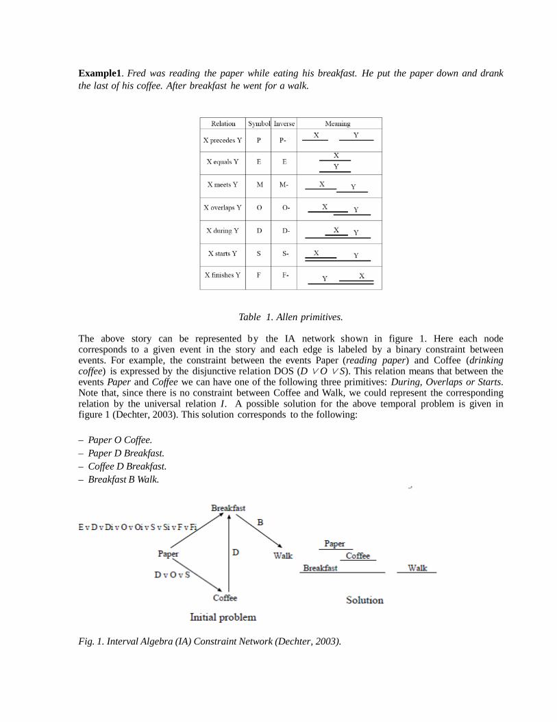
Example1. Fred was reading the paper while eating his breakfast. He put the paper down and drank the last of his coffee. After breakfast he went for a walk.

Table 1. Allen primitives. The above story can be represented by the IA network shown in figure 1. Here each node corresponds to a given event in the story and each edge is labeled by a binary constraint between events. For example, the constraint between the events Paper (reading paper) and Coffee (drinking coffee) is expressed by the disjunctive relation DOS (D ∨ O ∨ S). This relation means that between the events Paper and Coffee we can have one of the following three primitives: During, Overlaps or Starts. Note that, since there is no constraint between Coffee and Walk, we could represent the corresponding relation by the universal relation I. A possible solution for the above temporal problem is given in figure 1 (Dechter, 2003). This solution corresponds to the following: – Paper O Coffee. – Paper D Breakfast. – Coffee D Breakfast. – Breakfast B Walk.

Fig. 1. Interval Algebra (IA) Constraint Network (Dechter, 2003).

Probabilistic Symbolic Temporal Relations (PSTR) In probabilistic CSPs (Fargier, 1996), constraints can be certain or uncertain. Each uncertain constraint has a probability of its existence. For instance, Pr(C) = 0.7 means that the constraint C (involving a list of variables) has 70% chances to exist. In the case of IA networks, we associate these types of probabilities to the Allen primitives within a given uncertain relation rather than to the relation itself. More formally, we define a Probabilistic Symbolic Temporal Relation (PSTR) as follows. Definition 1.: Probabilistic Allen Primitive (PAP) A Probabilistic Allen Primitive (PAP) r is an Allen primitive that has a probability of its existence within a relation Rij between two events ei and ej. More precisely r has the following probabilities where 0 ≤ p ≤ 1. – Pr(r ∈ Ri j ) = p: the probability that r exists within Ri j – Pr(r ∈/ Ri j ) = 1 − p: the probability that r does not exist in Ri j The PAP r is certain (or completely known) if and only if Pr(r ∈ Rij ) = 1.0. In this case we simply call it Allen Primitive (AP). Definition 2.: Probabilistic Symbolic Temporal Relation (PSTR) Given a relation Rij between two events ei and ej ; and defined by the disjunction r1 ∨ r2 · · ·∨ rn where rn ≤ 13 and the rt is Allen primitive. R is a Probabilistic Symbolic Temporal Relation (PSTR) if and only if at least one of its ri’s is a PAP. The PSTR Rij is certain (or completely known) if and only if all its ri’s are certain (APs). In this latter case Rij is simply called Symbolic Temporal Relation (STR). The PSTR Rij can be formulated as follows. Rij = R1 ∨ ···∨ Rn where each Rk is an STR. Let us illustrate the above definitions through the following four examples. We will consider here the cases where the PSTR involves one or two primitives. The probability of a PSTR with more than two primitives can be computed in the same manner. Example2. Let us consider the story in example 1. The sentence “After breakfast he went for a walk” is certain and means that we have one primitive (B) in the relation R between the events Breakfast and Walk. B is certain (completely known) in the real world. Pr(R = B) = Pr(B V R) = 1.0. The solution to the problem including R must satisfy the relation B. Example 3. Let us consider again the story in example 1 but with the last sentence being uncertain: “After breakfast he might go for a walk”. Here too there is only one possible primitive (B) in R, but this time B exists in the real world with a given probability (0.6 for example). Pr(R) = Pr(B∈ R) = 0.6 Example 4. In example1, let us assume that we have the following additional information: “Fred does not start drinking coffee before he starts reading his paper. Usually he starts reading the paper first.” According to the above new information, there are now only two primitives (instead of three as shown in Figure 1) between the events Paper and Coffee. These primitives are O and S with O being the most probable one. Let us assign the following probabilities to each of these two primitives. Pr(S) = 0.6 and Pr(O) = 0.8. Using the above the PSTR R between Paper and Coffee is equal to one of three possible STRs as follows.

1. Pr(R = S) = Pr(S) × (1 − Pr(O)) = 0.6 × 0.2 = 0.12 2. Pr(R = O) = Pr(O) × (1 − Pr(S)) = 0.8 × 0.4 = 0.32 3. Pr(R = O ∨ S) = 0.6 × 0.8 = 0.48 The probability that R exists between Paper and Coffee is computed as follows. Pr(R) = Pr(R = O) + Pr(R = S) + Pr(R = O ∨ S) = 0.92 Probabilistic IA (PIA) Network Definition 3. A Probabilistic IA (PIA) network is a IA network where some disjunctive relations are PSTRs. Figure 2 shows the PIA network corresponding to example 1 with the additional information in examples 3 and 4. In the figure, the relations (Paper, Coffee) and (Breakfast, Walk) are PSTRs while the other two relations are STRs.

Fig. 2. PIA network corresponding to examples 1, 3 and 4.

Probable Worlds and Robust Solutions Definition 4. A probable world of a given PIA network P is a scenario (IA network) corresponding to replacing each PSTR of P by one of its possible STRs. A basic world is a probable world where all the selected STRs are APs. Let us consider the PIA network in Figure 2 with two PSTRs: (Paper,Coffee) and (Breakfast,Walk). A probable world (respectively basic world) can be obtained by replacing each of these two PSTRs by one of their STRs (respectively APs). Below we have the list of the three possible probable worlds where the first two are basic worlds. 1. W1: – Paper O Coffee. – Paper E ∨D∨D-∨O∨O-∨S∨S-∨F∨F- Breakfast. – Coffee D Breakfast. – Breakfast B Walk. 2. W2: – Paper S Coffee. – Paper E ∨D∨D-∨O∨O-∨S∨S-∨F∨F- Breakfast. – Coffee D Breakfast – Breakfast B Walk. 3. W3: – Paper OS Coffee. – Paper E ∨D∨D-∨O∨O-∨S∨S-∨F∨F- Breakfast. – Coffee D Breakfast. – Breakfast B Walk. Note that, in the above, W1 (respectively W2) is included in W3. Thus the set of solutions to W1 and W2 are included in the set of solutions to W3. Example 5. Let us consider another PIA network with two PSTRs C1 and C2 , and two STRs C3 and C4 defined as follows. – C1 = M ∨ S where Pr(M) = 0.2 and Pr(S) = 0.5. – C2 = O ∨ F where Pr(O) = 0.3 and Pr(F ) = 0.6. – C3 = P – C4 = Pi ∨ Oi C1 and C2 have each 3 possible temporal relations. One probable world can be defined, for example, by the following constraints {C1=M, C2 =O ∨ F, C3 =P, C4 =Pi ∨ Oi}. The total number of probable worlds will thus be equal to 9. Definition 5. The total number of possible worlds of a PIA network P can be computed as follows.

∏∈problemC

ii

C )dim( where dim(Ci) is the number of different situations of Ci.

Definition 6. Let us consider a given PIA network P and WS the set of probable worlds of P that can be satisfied by a given solution S. The robustness of S is computed as follows

∑∈

=WsWi

iWSRobustness )Pr()( where Ws = {probable worlds satisfied by S}

Definition 7. The most robust solution to a given problem P is the solution that has the highest degree of robustness. In other words, the above definition means that the most robust solution is the one that has the highest probability to satisfy the real world. Solving a PIA Network is an optimization problem that consists of finding the most robust solution. FINDING THE MOST ROBUST SOLUTION Example 6. Let us consider the PIA network of example 5. Here we have 4 basic worlds. 1. W1 = {C1 = M,C2 = O,C3,C4 } 2. W2 = {C1 = M,C2 = F,C3,C4 } 3. W3 = {C1 = S,C2 = O,C3,C4 } 4. W4 = {C1 = S,C2 = F,C3,C4 } Notice that the solutions of the above four basic worlds are all the solutions of the corresponding PIA network. Thus, in order to search for the most robust solution in a PIA network we can simply look for the most robust solution in the basic worlds only. The probability of a basic world is the product of the probabilities of all the uncertain primitives this basic world involves. For instance, the probability of each of the above four worlds is computed as follows. 1. Pr(W1 ) = Pr(M) × (1 − Pr(S)) × Pr(O) × (1 − Pr(F )) = 0.2 × 0.5 × 0.3 × 0.4 = 0.012. 2. Pr(W2 ) = Pr(M) × (1 − Pr(S)) × Pr(F ) × (1 − Pr(O)) = 0.2 × 0.5 × 0.6 × 0.7 = 0.042. 3. Pr(W3 ) = Pr(S) × (1 − Pr(M)) × Pr(O) × (1 − Pr(F )) = 0.5 × 0.8 × 0.3 × 0.4 = 0.048. 4. Pr(W4 ) = Pr(S) × (1 − Pr(M)) × Pr(F ) × (1 − Pr(O)) = 0.5 × 0.8 × 0.6 × 0.7 = 0.16. The most probable basic world is the basic world with the most probable uncertain primitives. In the above example, W4 is the most probable world. The robustness of a solution corresponds here to the probability of the basic world it satisfies. The most robust solution is the one that satisfies the most probable consistent world. Solving Algorithm Solving an IA network is an NP-hard problem that requires a backtrack search algorithm of exponential time cost (Mouhoub, 2004). In order to overcome this difficulty in practice, constraint propagation based on path consistency is used before and during the search in order to prevent earlier later failure. In the case of PIA networks we will also use backtrack search with path consistency performed before and during the search. Note that, when path consistency is used before the search it is applied to hard (certain) constraints only. If the path consistency fails then the PIA network is not consistent and there is thus no need to proceed with the search. In the case where the path consistency is successful then the hard constraints of the resulting network will have less Allen primitives which will reduce the size of the search space. More precisely, we propose the following branch and bound algorithm for finding the most robust solution. 1. Perform path consistency (van Beek, 1992) to the sub-network containing only the hard constraints. If the

sub-network is not path consistent return that the IA network is not consistent.

2. For each uncertain constraint, sort its primitives by decreasing order of their probability.

3. Following the forward check principle (Haralick, 1980), pick a constraint, assign to it one of its Allen

primitives and run the path consistency algorithm on the sub-network containing the newly assigned constraint and the non assigned ones. If path consistency fails then assign another primitive to the current constraint or backtrack to the previous assigned constraint if the current constraint does not have any another primitive to assign. If the path consistency is successful, select another constraint and redo the same process until all the constraints are assigned in which case we obtain a solution otherwise return that the PIA network is not consistent. If a solution is obtained, compute its robustness (the probability of the complete assignment it satisfies) and assign the result to the lower bound (LB).

4. The rest of the search space is then systematically explored as follows. Each time the current constraint is assigned a primitive, if this constraint is uncertain (PSTR) then an overestimation of the robustness of any possible solution following this decision is computed and used as an upper bound (UB). If UB < LB then the current uncertain constraint is assigned another value or backtrack to the previous constraint if all the primitives have been explored. The overestimated robustness is the product of the probabilities of all the assigned primitives plus the product of the max probabilities of the uncertain constraints that are not yet assigned. The max probability of a non assigned uncertain constraint corresponds to the largest probability of its primitives.

PROBABILISTIC NUMERIC TEMPORAL NETWORK In this section we show how to handle uncertain domains in the TemPro framework. An algorithm for dividing domains into non-overlapping areas is reported. We also examine the calculation of the robustness of solutions in different probable worlds. At the end, we present the branch-and-bound algorithm for searching the most robust solution in the TemPro framework with uncertainty. TemPro Framework TemPro (Mouhoub, 2004) transforms a temporal problem under qualitative and quantitative constraints into a binary CSP where constraints are disjunctions of Allen primitives and variables, representing temporal events, are defined on domains of time intervals. Each event domain (called also temporal window) contains the Set of Possible Occurrences (SOPO) of numeric intervals the corresponding event can take. The SOPO is the numeric constraint of the event. It is expressed by the fourfold: [earliest start, latest end, duration, step] where: earliest start is the earliest start time of the event, latest end is the latest end time of the event, duration is the duration of the event and step is the discretization step corresponding to the number of time units between the start time of two adjacent intervals. Each interval is shown as (StartTime, EndTime), in which StartTime is the actual start time of the event and EndTime is the actual end time which is the summation of StartTime and duration of the event. StartTime of each event should be selected based on the unary constraints it is involved in. Hence, if we consider the TemPro model, domain of StartTime of event i would be earliest start+(X ×step) where X ranges in the interval of [0, (latest end - earliest start - duration)/step]. Extending TemPro with Uncertainty Uncertainty of Domains In the STPU (Peintner, 2007), the uncertainty is mainly focused on the duration of some uncertain events. In addition to duration, there could also be some other uncertainty for one event, such as the earliest start time (INF) and latest finish time (SUP). In uncertain and dynamic environment, the INF and SUP of an event are affected by some external factors. Let us consider the following example.

Example 7: Uncertain INF and SUP of an event. Everyday Bob takes bus to his company. Occasionally, the bus is full and he has to call a taxi. The bus arrives at the company at 8:30 and the taxi arrives at the company at 8:20. Bob normally finishes his job in 12:00. However, his manager Tom may want to talk with him after 12:00, which will take 60 minutes. Bob doesn’t know whether Tom wants to talk with him before 12:00. In the above example, the earliest start (INF) of event workInOffice depends on which vehicle Bob takes. Suppose 8:00 is the zero point in the time line. If Bob takes the bus, the INF for workInOffice would be 30 (corresponding to 8:30). If he takes a taxi, the INF for workInOffice would be 20. The latest finish (SUP) of event workInOffice is also associated with some uncertainty. If Tom does not want to talk with him, the SUP for workInOffice would be 240. Otherwise, the SUP of workInOffice would be 300. With the uncertainty in domains of events, both the INF and SUP are no longer single time points, but probability distributions of several possible time points. For example, there are three possible earliest start time points: 20, 30 and 40 for a single event E1. These earliest start time points are caused by some external factors, as the INF of the event workInOffice in the above example. The priori probability of each earliest start can be computed by statistics or estimated by induction. Assume E1 has a length of 15 and the step is 1 unit. The probabilities of these three INF are listed as follows. Pr {E1 = [20, SUP, 15, 1]} = 0.2 Pr {E1 = [30, SUP, 15, 1]} = 0.3 Pr {E1 = [40, SUP, 15, 1]} = 0.5 The uncertainty of the latest finish (SUP) can be presented in a similar way. Assume that three possible latest end time points 45, 60 and 80 exist for E1. Their probabilities can be described in a similar form. Pr {E1 = [INF, 45, 15, 1]} = 0.4 Pr {E1 = [INF, 60, 15, 1]} = 0.1 Pr {E1 = [INF, 45, 15, 1]} = 0.5 With the addition of uncertain INF and SUP, the domain of one event is no longer a certain time frame, but rather a dynamic time window. For the previous example of event E1, we have 3 different INF and 3 different SUP. Therefore, there are 9 (33) possible domains in total. [20, 45, 15, 1], [20, 60, 15, 1], [20, 80, 15, 1] [30, 45, 15, 1], [30, 60, 15, 1], [30, 80, 15, 1] [40, 45, 15, 1], [40, 60, 15, 1], [40, 60, 15, 1]

More formally, the set of domains of event E can be defined as: D = [INFi, SUPj, DUR, STEP] where INFi and SUPj are the possible values for INF and SUP, respectively. Continuous and Discrete Probabilities The earliest start (INF) and the latest finish (SUP) in a SOPO define the time domain for a specific event. In the previous subsection, we assumed that the probability distribution for INF and SUP are discrete. The discrete probability distribution is applied to handle uncertainty caused by discrete external factors. For example, in the previous example, full and empty are the only two discrete possible states of the bus. The actual state of the bus affects the INF of the event workInOffice. In some real world applications, however, the determinant external factor may be a continuous variable. For example, the bus may arrive at the office within a range between 8:25 and 8:35 with a continuous probability distribution, which affects the corresponding event workInOffice. Since TemPro can only handle discrete time points, we have to

discreterize the continuous distribution. First, the continuous distribution is divided into several areas in its range. The mid-points of each area are used as the representative values for that area. Then, cumulative probabilities are calculated for the continuous distribution in each area. Each cumulative probability will be associated with the corresponding midpoint to generate a discrete distribution. Uncertain Domains and Probable Worlds Calculation of Probabilities of Uncertain Constraints Given the probabilities of uncertain INF and SUP, the probability of each possible domain (SOPO) for an event can be calculated. In the above example, we have two sets of INF and two sets of SUP. Assume the INF and SUP are caused by independent external factors, we can calculate the probabilities of the SOPO for E1 as follows. Pr (E1 = [20, 45, 15, 1]) = Pr(E1= [20, SUP,15,1]) × Pr(E1 = [INF, 45, 15, 1]) = 0.2 × 0.4 = 0.08 Pr (E1 = [20, 60, 15, 1]) = Pr(E1 = [20,SUP,15,1]) × Pr(E1 = [INF,60,15,1]) = 0.02 Pr (E1 = [20, 80, 15, 1]) = Pr(E1 = [20,SUP,15,1]) × Pr(E1 = [INF,80,15,1]) = 0.01 Pr (E1 = [30, 45, 15, 1]) = Pr(E1 = [30,SUP,15,1]) × Pr(E1 = [INF,45,15,1])= 0.12 Pr (E1 = [30, 60, 15, 1]) = Pr(E1 = [30,SUP,15,1]) × Pr(E1 = [INF,60,15,1]) = 0.03 Pr (E1 = [30, 80, 15, 1]) = Pr(E1 = [30,SUP,15,1]) × Pr(E1 = [INF,80,15,1]) = 0.15 Pr (E1 = [40, 45, 15, 1]) = Pr(E1 = [40,SUP,15,1]) × Pr(E1 = [INF,45,15,1]) = 0.20 Pr (E1 = [40, 60, 15, 1]) = Pr(E1 = [40,SUP,15,1]) × Pr(E1 = [INF,60,15,1]) = 0.05 Pr (E1 = [40, 80, 15, 1]) = Pr(E1 = [40,SUP,15,1]) × Pr(E1 = [INF,80,15,1]) = 0.25 The sum of these probabilities is equal to 1. More formally, the probability of each SOPO is calculated with the following formula. Pr{E = [INFi , SU Pj , DU Ri , ST E Pi ]} = Pr{INF = INFi } × Pr{SU P = SU Pj }

∑ ==ji

ji STEPDURSUPINFE,

0.1]},,,[Pr{

Dividing Domains into Non-Overlapping Areas In the above example, there are nine possible domains (SOPOs) for E1. However, these domains are not separately distributed along the time line. Some of them such as [30, 60, 15, 1] and [40, 80, 15, 1] overlap each other. Actually, with three INF and three SUP for event E1, we can order them as follows. INF1 < INF2 < INF3 SUP1 < SUP2 < SUP3 We can thus divide the possible domains of E1 into 5 non-overlapping areas. A1: [INF3, SUP1] A2: [INF2, INF3 + DUR] A3: [INF1, INF2 + DUR] A4: [SUP1 - DUR, SUP2] A5: [SUP2 - DUR, SUP3] Figure 3 illustrates the above overlapping.

Fig.3. Dividing domains into non-overlapping areas

By dividing the entire possible domains into non-overlapping areas, a solution containing an event in one area will not be contained in any other areas. Furthermore, these non-overlapping areas cover all the possible assignments of each event in the final solution. Therefore, we can consider the assignment of events in each area. In order to calculate the probabilities of solutions, these non-overlapping areas must also not be overlapped by the original possible SOPOs. In other words, for each possible SOPOi (i=1 to 9) in the above example, Ai (i=1, 2, 3, 4, 5) must be either included in or excluded from SOPOi. Consider the following example (see figure 5) for an incorrect way of dividing domains into non-overlapping areas.

Fig 4. An incorrect way for dividing domains into non-overlapping areas In Figure 5 the domains are divided into two non-overlapping areas [INF1, SUP1] and [SUP1−DUR, SUP1]. Since the area [INF1, SUP1] overlaps the original possible SOPO [INF2, SUP2], this dividing strategy is not suitable for computing the probabilities of solutions. In the above example, SUP (SUP1, SUP2, SUP3) are greater than INF (INF1, INF2, INF3). In some other cases, INF and SUP may be mixed on the time line (as shown in Figure 6. The dividing algorithm is shown in Figure 7.

Fig.5. Another way of dividing with mixed INF and SUP

Function DivideAreas (ListofSOPOs)

1. Sort INF and SUP. INF1 < INF2 < INFm, SUP1 < SUP2 < … < SUPn 2. AreaList ← empty 3. L ← empty // L contains minimal areas 4. for each SOPO S in ListofSOPOs do 5. if no other INF or SUP are in [INFS, SUPS] 6. L ← L ∪{S} 7. end for 8. RemainList ←the combinations of [INF, SUP] except [INF1, SUPn] 9. CurrentCoverage ← empty; // CurrentCoverage is the union of current generated areas

// e.g. we have two areas [25,26], [22,27], then it will be [22,25]

10. while L is not empty do 11. NextDomainLength ← positive infinity 12. NextDomain ← empty 13. for each SOPO R in RemainList do 14. if R ⊇ CurrentCoverage and length(R) < NextDomainLength then 15. NextDomainLength = length(R) 16. NextDomain = R 17. end for

Fig. 6. The algorithm of dividing domains into non-overlapping areas

Probabilities of areas In Figure 3, we defined five non-overlapping areas. There is one begin time point and one end time point for each area (Ai = Ai-begin, Ai-end). For each of its possible SOPO (INFi, SUPj), if INFi < Ai-begin < Ai-end < SUPj, then Ai (INFi, SUPj), which implies that the solution in Ai is also a solution in (INFi, SUPj). Since Ai must be contained in either one or more SOPOs, we can use the following formula to calculate the probability of area Ai to be included in the actual domain for the corresponding uncertain event. Pr(Ai is included in the actual domain) = ∑ Pr(INFi, SUPj) where Ai∈(INFi, SUPj) For example, A1 is the subset of nine possible SOPOs (see Figure 3), so the probability of A1 to be included in the actual domain is 1.0. In other words, if we can find a solution in A1, the probability of this solution to fall in the actual domain will be 1.0. A2 is the subset of [INF2, SUP1], [INF2, SUP2] and [INF2, SUP3]. So the probability of A2 to be included in the actual domain is 0.12 + 0.03 + 0.15 = 0.30. Probable Worlds Given the possible domains of each event, we can define probable worlds in numeric TCSPs as combinations of domains for each event. For events with certain INF and SUP, the domains are just the given INF and SUP. For events with uncertain INF and SUP, however, one of the possible domains will be picked up.

ProbableWorld = {D1, D2, . . . , Dn, {Dcertain}, {C}} where C is the constraint and Di is the specific domain of each uncertain event. Let us consider the following example. Example 8. Probable world in the TemPro model We have three events E1, E2 and E3. E1 and E2 are traditional events with certain INF and SUP. E3 and E4 are events with uncertain INF and SUP. Their SOPOs are given as follows. E1 = [20, 60, 15, 1] E2 = [30, 70, 25, 1] E3= [INFE3, SUPE3, 40, 1] Pr (INFE3 =10) = 0.4, Pr (INFE3 = 20) = 0.6, Pr (SUPE3 = 100) = 0.3, Pr (SUPE3 = 120) = 0.7 E4= [45, SUPE4, 35, 1] Pr (SUPE4=90) = 0.2, Pr (SUPE4=130) = 0.8 Here we use the non-overlapping areas generated by the dividing algorithm to build probable worlds. The total number of probable worlds is the product of the number of generated non-overlapping areas of each uncertain constraint. For example, in the above example, we have three areas for E3 and two areas for E4. So the total number of probable worlds is 3×2 = 6. The set of these six probable worlds is called set of basic probable world. More formally, suppose the number of certain events is m while the number of uncertain events is n. Set of basic probable worlds = {[INF, SUP]i , Areaj} | 1 < i < m, 1 < j < n [INF, SUP]i is one SOPO of certain events and Areaj is one area of uncertain events. One probable world WP in the set of basic probable worlds is E1, E2, E3 = [10, 60], E4 = [55, 80]. In this world, we use the area AreaE3 [10, 60] for E3 and the area AreaE4 for E4. Their probabilities are listed below. Pr (AreaE3 is included in the actual domain of E3) = 0.4 Pr (AreaE4 is included in the actual domain of E4) = 0.8 Then the probability of WP containing the real domains of E3 and E4 is Pr (WP is included in the actual domains of both E3 and E4) = Pr (AreaE3 is included in the actual domain of E3) × Pr (AreaE4 is included in the actual domain of E4) = 0.4 × 0.8 = 0.32 Therefore, if we find a solution Sol to this probable world WP, the probability of Sol to fall in the real domain of E3 and E4 will be 0.32. Since the actual problem is determined by uncertain events, 0.32 can also be viewed as the probability of Sol to satisfy every constraint in the real world. Robustness of Solutions Given the set of basic probable worlds, our goal is to find the most robust solution. We define the robustness of a solution as the probability of this solution to satisfy every constraint in the real world. This probability can be illustrated as follows. Suppose we have a numeric TCSP P with uncertainty. If P happens n times and one of the solutions satisfies the problem in 0.6 × n times, the probability of P satisfying the real world is 0.6. By using non-overlapping areas to generate probable worlds, the solutions for each probable world do not overlap each other. The solution to one probable world is not the solution for any other probable world. So we can consider the solution to each probable world and calculate the robustness of each solution. More formally, it can be calculated using the following formula:

Robustness of s = Pr (Wi is included in the actual domains for all the uncertain events) where s satisfies Wi and Wi is in the set of probable worlds For example, if we have four different worlds W1, W2, W3, W4 and four corresponding solutions S1, S2, S3, S4. The probability of each world is listed below. Pr (W1 is included in the actual domain for all the uncertain constraints) = 0.6 Pr (W2 is included in the actual domain for all the uncertain constraints) = 0.5 Pr (W3 is included in the actual domain for all the uncertain constraints) = 0.8 Pr (W4 is included in the actual domain for all the uncertain constraints) = 0.2 The robustness of S1, S2, S3, S4 is 0.6, 0.5, 0.8, 0.2, respectively. S3 is the most robust solution due to its highest probability to be the solution for the real problem. The main task of solving numeric TCSPs with uncertain events is to find the solution with the highest degree of robustness. Solving the Problem Removing inconsistent areas We discussed earlier the algorithm for dividing domains into non-overlapping areas. However, we did not consider the validity of all the generated areas. According to the values of the lower boundary and the upper boundary, there may be some inconsistent areas. For example, we have an area of an uncertain event E1 [A1-begin, A1-end] with a probability of 0.8 to be included in the actual domain. The length of the event is specified by DURATION. If A1-end − A1-begin < DURATION, there will be no solutions in this domain even if it is associated with a probability of 0.8. Therefore, all the probable worlds that contain this area for event E1 should be removed from the set of basic probable worlds. By removing inconsistent areas, the number of corresponding probable worlds can be reduced exponentially, which will improve the efficiency of the solving algorithm. Branch and bound algorithm The intuitive method consists of sorting all the probable worlds by their probabilities. Then we try to find a solution to the most probable world. If a solution is found, it will be the most robust solution. If no solution is found, we switch to the next most probable world. A more effective algorithm is to use branch-and-bound through the search for the most robust solution. The different steps of the algorithm are shown below. 1. Perform path consistency check for the symbolic constraints in the problem (see Figure 3). If the

problem is inconsistent, return NO SOLUTION.

2. For all the constraints involving certain events, perform the numeric to symbolic conversion we proposed in (Fargier, 1996) to remove the Allen primitives that are inconsistent with the numeric information.

3. Divide the uncertain domains of events into non-overlapping areas. For each event with uncertain domains, maintain a list of areas L = {A1 , A2 , . . . , Am}. Set the lower bound LB to 0.

4. Remove those areas inconsistent with the problem, i.e., Areaend − Areabegin < DURATION.

5. Calculate the probability of each area to be included in the actual domain of each uncertain event.

6. Pick an uncertain event and select an area from L. An overestimation of the robustness of any possible solution falling in the current assigned areas is calculated and used as the upper bound UB (see below). If UB < LB, select another area for the current uncertain event or backtrack to

the previous uncertain event if all the areas for this event have been explored.

7. Perform arc-consistency check (Mackworth, 1977) for current uncertain events with assigned domains. If the arc consistency fails, select another area for the current uncertain event or backtrack to the previous uncertain event if all the areas for this event have been explored.

8. For all the constraints related to this uncertain event, perform numeric to symbolic conversion by using the currently assigned area.

9. Repeat 6 to 8 until all the uncertain events have been assigned areas.

10. If every uncertain event has been assigned a specific area, search for a solution to the problem. Calculate the robustness of the solution. If it is larger than LB, update LB with the value. If there is no solution or the probability is less than LB, backtrack and go to step 4.

11. If all the areas of uncertain events have been tried and no solution is found, return NO SOLUTION.

The overestimation of the robustness is the product of probabilities of already assigned areas and the maximum probabilities of areas for all the non-assigned uncertain events. For example, there are four uncertain events E1, E2, E3, E4 and there are two assigned areas, A1 for E1, A2 for E2. The probabilities of A1 and A2 are Pr (A1 is included in the actual domain of E1) = 0.8 Pr (A2 is included in the actual domain of E2) = 0.6 As shown below, we have three areas for event E3 and two areas for event E4. Pr (A3-1 is included in the actual domain of E3) = 0.3 Pr (A3-2 is included in the actual domain of E3) = 0.2 Pr (A3-3 is included in the actual domain of E3) = 0.9 Pr (A4-1 is included in the actual domain of E4) = 0.5 Pr (A4-2 is included in the actual domain of E4) = 0.8 We use Pr(Ai) here to simplify Pr(Ai is included in the actual domain). The overestimation of the robustness of solutions in any probable worlds that contain A1 and A2 can be calculated as follows. UB = Pr (A1) × Pr (A2) × max (Pr (A3-1), Pr (A3-2), Pr (A3-12)) × max (Pr (A4-1), Pr (A4-2)) = 0.8 × 0.6 × 0.9 × 0.8 = 0.3456 The pseudo code of the solving method is shown in Figure 7.

// Problem is the numeric TCSP with uncertainty, FCEvtLst is the list of fixed events // UCEvtLst is the list of uncertain events, Graph is the constraint graph of the this TCSP Function SolveUncertainNumericTCSP (Problem, FCEvtLst, UCEvtLst, Graph) 1. curSol = NULL // curSol is the current solution 2. lowerBound = 0 3. upperBound = 0 4. oldGraph = graph 5. if DPC (oldGraph) then// check path consistency 6. return NO_SOLUTION 7. for each ei in FCEvtLst 8. for each ej in FCEvtLst 9. Num2Sym(ei, ej) // perform the numeric to symbolic conversion 10. end for 11. areaList = divideAreas(FCEvtLst) // divide uncertain events into non-overlapping areas 12. for each area in areaList 13. if SUP(area) - INF(area) < DURATION(area) then 14. remove(area) // remove the area from the areaList 15. probListAreas = calculateProbability(areaList) 16. end for 17. while (notAllEventsExplored(Problem)) // if not all scenarios visited 18. pushScenario(oldGraph) // save the current scenario 19. event = removeNextEvt(UCEvtLst, newGraph) 20. // removing one event from the list of uncertain events, forming newGraph 21. if (noAreas(event)) then // no areas left, backtrack 22. popScenario(oldGraph) 23. goto 17 24. assignNextArea (event, newGraph) 25. // pick one area as the domain for this event, forming the new graph 26. if AC3.1(newGraph) then 27. popScenario(oldGraph) 28. goto 17 29. upperBound = estimateRobustness (newGraph) 30. if (upperBound < lowerBound) then 31. popScenario(oldGraph) // backtrack, cutting branches 32. goto 17 33. constraintList = allRelatedConstraints(event); 34. // constraintList is the list of all constraints related to this event 35. for each ei in constraintList 36. for each ej in constraintList 37. Num2Sym(ei, ej) // perform the numeric to symbolic conversion 38. end for 39. if allAreasAssigned() then // if one area is specified for each event 40. // using backtrack search to find a solution 41. if (BTNumericTCSP(newGraph, curSol)) then // if one solution is found 42. newRobustness = calculateRobustness(newGraph, curSol) 43. if newRobustness < lowerBound then 44. lowerBound = newRobustness 45. else 46. popScenario(oldGraph) 47. goto 17 48. end while

Fig. 7. Pseudo code for solving symbolic TCSPs with uncertainty

PC First Solution 10%

uncertain 20%

uncertain 30% uncertain

N = 40 0.05 3.204 3.495 3.675 4.689 N = 60 0.15 6.714 7.21 7.93 8.35

N = 80 0.35 15 16.5 17.2 19 N = 100 0.66 33 35 41 45

N = 120 1.11 48 52 54 57 N = 150 2.10 62 69 74 81 N = 180 3.59 187 201 231 254 N = 200 4.92 312 352 418 516

Table 2. Time performance of the solving method.

EXPERIMENTATION In order to evaluate the solving method we propose, we have performed several tests on randomly generated consistent PIA networks. The experiments are performed on a PC Pentium 4 computer under Windows XP system. All the procedures are coded in C++. A consistent IA network of size N (N is the number of variables) is randomly generated as follows. We first randomly generate a numeric solution (set of N numeric intervals), extract the Allen primitives that are consistent with the numeric solution and randomly add other primitives to get the set of constraints of the generated problem. To generate a PIA network having a percentage p of uncertain constraints, we randomly pick p × C constraints (where C is the total number of constraints) and randomly assign probabilities to all the primitives within each selected constraint. Table 2 presents the results of tests conducted on randomly generated PIA networks. For each test we run the solving method on 10 instances of the same problem and we take the average running time in seconds. The generated problems are complete PIA networks (all constraints are different from the universal relation I). Thus, the number of constraints is equal to N× (N−1) / 2 where N is the number of variables. The second column corresponds to the time needed by the path consistency algorithm performed before the backtrack search. The third column corresponds to the time to find the first solution. The fourth, fifth and sixth columns correspond respectively to the time needed to find the most robust solution for problems where 10%, 20% and 30% of their constraints are uncertain. As we can see from the test results, after finding the first solution, not much effort is needed to find the most robust one while there is actually a large number of probable worlds and their corresponding solutions especially in the case of large size problems. This is due to the branch and bound algorithm that prunes the search space significantly and also to the fact that the first solution obtained is of good quality which sets the lower bound of the algorithm to a good value. CONCLUSION In this paper we have proposed a new framework for handling uncertain symbolic and numeric temporal information. At the symbolic level, the uncertainty is represented by the probability of the existence of each Allen primitive within its uncertain constraint. A PIA network P will thus involve a list of worlds and solving P consists of finding a solution for the most probable ones. This is an optimization problem that we tackle using a branch and bound algorithm based on temporal constraint propagation. Experimental study on randomly generated uncertain temporal networks demonstrates the efficiency of our solving method. At the numeric level, our TemPro framework is extended to handle uncertain

domains. An algorithm for dividing domains into non-overlapping areas is proposed. This algorithm guarantees that the generated possible worlds do not intersect. Probable worlds are then constructed by combining these areas. A new branch and bound algorithm, we propose, is finally applied to find the most robust solution. FUTURE RESEARCH DIRECTIONS In the near future we intend to see how handling uncertainty can be done in a dynamic environment (when temporal constraints are added and removed during the resolution of the probabilistic temporal problem). Another perspective is to consider (instead of a branch and bound based algorithm) approximation methods such as Stochastic Local Search (SLS), Genetic Algorithms (GAs) and Ant Colony Algorithms (ACAs). While these techniques do not always guarantee an optimal solution to the probabilistic temporal problem, they are very efficient in time (comparing to branch and bound) and can thus be useful if we want to trade the optimality of the solution for the time performance. REFERENCES Allen, J. (1983). Maintaining knowledge about temporal intervals. CACM, 26(11), 832–843. Badaloni, S. & Giacomin, M. (1999). A fuzzy extension of Allen’s Interval Algebra. In Proc. of the 6th Congress of the Italian Assoc. for Artificial Intelligence, E. Lamma and P. Mello, Eds., pp. 228–237. Baptiste, J. & Le Pape, C. (1995). Disjunctive constraints for manufacturing scheduling: Principles and extensions. In Third International Conference on Computer Integrated Manufacturing, Singapore. Dean, T. (1989). Using Temporal Hierarchies to Efficiently Maintain Large Temporal Databases. JACM, 686–709. Dechter, R. (2003). Constraint Processing. Morgan Kaufmann. Dechter, R., Meiri, I. & Pearl, J. (1991). Temporal Constraint Networks. Artificial Intelligence, vol. 49, 61–95. Fargier, H. , Lang, J. & Schiex, T. (1996). Mixed constraint satisfaction: A framework for decision problems under incomplete knowledge. In the 13th National Conference on Artificial Intelligence (AAAI-96), pp. 175–180, ACM Press, New York. Golumbic, & Shamir, R. (1993). Complexity and algorithms for reasoning about time: a graphic-theoretic approach. Journal of the Association for Computing Machinery, 40(5):1108–1133. Haralick, R. & Elliott, G. (1980). Increasing tree search efficiency for Constraint Satisfaction Problems.” Artificial Intelligence, 14, 263–313. Hwang & Shubert, L. (1994). Interpreting tense, aspect, and time adverbials: a compositional, unified approach. In Proceedings of the first International Conference on Temporal Logic, LNAI, vol 827, pp. 237–264, Berlin. Mackworth, A.K. (1977). Consistency in networks of relations. Artificial Intelligence, 8, 99–118. Marin, R. & Cardenas, M., Balsa, M. & Sanchez, J. (1997). Obtaining solutions in fuzzy constraint networks. International Journal of Approximate Reasoning, 16, 261–288. Morris, P. & Muscettola, N. (2000). Execution of temporal plans with uncertainty. AAAI 2000, pp. 491–496. Mouhoub, M. (2004). Handling Numeric and Symbolic Time Information. Artificial Intelligence Review, 21, 25–56.

Peintner, B., Venable, K.B. & Yorke-Smith, N. (2007). Strong Controllability of Disjunctive Temporal Problems with Uncertainty. CP 2007, pp 856–863, 2007. Ryabov, V. & Trudel, A.. (2004). Probabilistic temporal interval networks. In TIME 2004, pp. 64–67. Tsamardinos, Vidal, T. & Pollack, M.E. (2003). CTP: A New Constraint-Based Formalism for Conditional Temporal Planning. Constraints, 8(4):365–388. van Beek, P. (1992). Reasoning about qualitative temporal information, Artificial Intelligence, 58, 297–326. Vidal, T. & Fargier, H. (1999). Handling consistency in temporal constraint networks: from consistency to controllabilities. Journal of Experimental and Theoretical AI, 11, 23–45. Vidal, T., & Ghallab, M. (1996). Dealing with uncertain durations in temporal constraint networks dedicated to planning. In ECAI-1996, pp. 48–52. Vilain, M. & Kautz, H. (1986). Constraint propagation algorithms for temporal reasoning, in AAAI’86, Philadelphia, PA pp. 377–382. Walsh, T. (2002). Stochastic constraint programming. In Proceedings of the 15th European Conference on Artificial Intelligence (ECAI-02), Lyon, France.

Key Terms & Definitions Backtracking algorithm. A systematic search method that explores the search space in a depth first manner. In the case of a CSP, the backtracking algorithm extends a partial solution (corresponding to a partial assignment) toward a complete one. Branch and bound (BB). A backtracking algorithm for solving discrete optimization problems. BB explores a search space in a systematic way looking for the optimal solution. Lower and upper bounds are used to filter potential solutions that will not lead to the optimal one. Constraint Satisfaction Problem (CSP). A problem defined with a list of variables, each taking values in discrete and finite domains and a list of relations restricting the values that the variables can simultaneously take. Decision Problem. A problem where the solving algorithm has only two possible outputs, yes or no. Event. A preposition that holds over a time interval. Probabilistic Constraint Satisfaction Problem (PCSP). A CSP where each constraint has a probability to exist in the problem. Search Space. The set of all potential solutions. Systematic Search Method. A solving method, to a decision problem, that explores the search space in a systematic manner. The systematic search method guarantees to find a solution if it exists. Temporal Constraint Satisfaction Problem. A CSP where the constraints or values are temporal.