probabilistic topic model for hybrid recommender systems: a
TRANSCRIPT
Probabilistic Topic Model for Hybrid Recommender
Systems: A Stochastic Variational Bayesian Approach
Asim Ansari Yang Li Jonathan Z. Zhang1
July 2016
1Asim Ansari is the William T. Dillard Professor of Marketing at Columbia Business School, Yang Liis Assistant Professor of Marketing at Cheung Kong Graduate School of Business in Beijing, and JonathanZ. Zhang is Assistant Professor of Marketing at University of Washington in Seattle.
Abstract
Recommendation systems are becoming increasingly popular and useful in e-commerce and dig-ital product contexts that involve heterogeneous consumers and a vast collection of products. Thiscreates representational challenges as features that adequately describe the products are often notreadily available. User-generated content in the form of product reviews or product tags can beleveraged to obtain rich representations for subsequent product recommendation and targeting. Inthis paper we develop a novel covariate guided supervised topic model (CGSTM) that succinctlycharacterizes products in terms of latent topics and specifies consumer preferences through thesesemantic features. At the same time, recommendation contexts generate big data problems stem-ming from data volume, variety and veracity, such as our setting that includes massive textual andnumerical data. To overcome the computational challenges due to the combination of big data anda complex model, we develop a novel stochastic variational Bayesian (SVB) framework to achievefast, scalable and accurate estimation. We use our SVB approach to estimate our model on adataset of 8.87 million movie ratings from 111,793 customers and 233,268 textual movie tags. Theresults show our model generates much better predictions than those from a benchmark model, andyields interesting insights about movie preferences. We also illustrate how our model can be usedfor targeting recommendations to particular users, and how it can support personalized search bydetermining relevant products and by generating a personalized ranking of these relevant products.
Keywords: Hybrid Recommendation Models, Personalized Search, User-Generated Content, Prob-abilistic Topic Models, Big Data, Scalable Inference, Stochastic Variational Bayes.

1 Introduction
Over the past decade, e-commerce firms, online retailers, and digital content providers such as
Amazon, Netflix and New York Times have become increasingly reliant on recommender systems
to target products and digital content to users. Recommender systems are particularly useful in
environments that are characterized by a large number of users who face a vast array of products to
choose from. In such contexts, there is considerable heterogeneity in user preferences for product
attributes and the large number of products implies that users are often unaware or uncertain of
products that might appeal to them. Moreover, such environments are often constantly evolving as
new users and new items are added on a regular basis. Firms therefore use recommender systems
to offer personalized suggestions to users. This task hinges upon the recommender system’s ability
to capture the heterogeneous preferences of current users based on their previous product ratings
or product choices and to use such information to predict their liking of new items.
Recommendation systems need to overcome various modeling and computational challenges to
successfully predict preferences and recommend products. Such systems often operate on a sparse
database in which each consumer rates only a few items and each product is rated or chosen by
only a few customers. The paucity of data for most consumers implies that it is critical to borrow
information from other consumers in order to predict the preferences of a given consumer, and
therefore some type of shrinkage mechanism is needed to model customer heterogeneity. The large
number of products within a database also poses challenges in representing these in terms of their
underlying features. In many marketing situations, such feature representations are unavailable,
or are at best partially available, as considerable domain expertise is needed for firms to manually
supply detailed content descriptors for each product. Yet, a rich representation of products in terms
of their attributes is crucial for properly modeling preference heterogeneity. Thus many systems
rely on some sort of automatic feature extraction. In this research, we show how user-generated
content that represents the “voice of the customers” can be leveraged to automatically extract
features that are most predictive of preferences. Finally, recommender systems need to overcome
various cold start problems associated with new users and new items.
Apart from the modeling challenges, typical recommendation contexts generate big data com-
putational challenges stemming from data volume, variety and veracity. While personalization

focuses on a given user or a given product, large data volume that results from a massive user base
and a vast product mix is critical for recommendation success, as it facilitates borrowing of infor-
mation and enriches representation of products. However, this also results in scalability challenges,
particularly so if complex probabilistic representations are needed to fully capture the information
content in the data. Moreover, the application of user-generated content such as online texts and
tags implies a curse of dimensionality, which needs to be tackled via appropriate dimensionality
reduction procedures. Thus, scalable methods that are capable of estimating probabilistic models
involving many latent variables on large datasets of variegated forms are needed.
In this paper, we develop a novel hybrid model-based recommendation framework that ad-
dresses the above representational challenges. In addition, we develop a novel stochastic variational
Bayesian approach for estimation that overcomes the scalability challenges associated with large
volume and high dimensionality. Specifically, we leverage crowd-sourced textual descriptions of
products, such as user-generated tags, to construct probabilistic content descriptors of products.
This alleviates the often onerous requirement for the firm-provided product attributes – an issue
that bedevils most content filtering recommendation systems. We construct a supervised proba-
bilistic topic model that transforms the “voice of the customer” about products and automatically
infers latent product features that not only summarize the semantic content within the tags/words,
but also simultaneously predict product ratings. In our model, the topics capture the semantic
structure of the textual representation of the products and allow automatic dimension reduction of
the vast vocabulary underlying the textual descriptions. More importantly, consumer preferences
are specified in terms of these latent topics in our model. As we jointly model both the textual
data as well as the product ratings, these latent topics are inferred to be the most predictive of
user preferences. In addition, we allow firm specified covariates, when available, to guide the al-
location of products to topics. This results in a recommendation system that leverages preference
heterogeneity over rich user-generated content representations in a seamless manner.
Specifically, we develop a covariate-guided supervised topic model to relate the textual descrip-
tion of products to the user ratings. Our model extends the supervised latent Dirichlet allocation
model (SLDA; Blei and McAuliffe 2007) in several directions to capture the unique characteristics
of the recommendation context. Recommendation datasets often have a cross-nested dependency
structure as a given user rates multiple products and each prodcut is rated by multiple users. In
2
our model each product description (e.g., a document in the topic model) is associated with mul-
tiple product ratings given by many different users. This is distinct from typical supervised topic
models in which each document is rated by a single user – such models are therefore more suitable
for sentiment analysis of reviews, but are not rich enough to represent the preference heterogeneity
that is crucial in making successful recommendations. We also account for preference heterogeneity
over topics and explicitly take into account the cross-nested structure of the data. Finally, we use
firm specified product covariates to guide the allocation of latent topics to products. This allows
us to tackle the cold-start problem associated with new products.
We apply our modeling framework to the context of personalized movie recommendations. We
believe that the experiential nature of movie products is more amenable for using automatic feature
extraction from crowd-sourced customer opinions, especially because standard content descriptors
such as movie genre are not rich enough to flexibily capture the numerous reasons why certain
movies appeal to particular consumers. While we use crowd-sourced tags to generate textual
representations for movies, such representations can also be obtained from other naturally occurring
information sources on the Internet, such as Wikipedia, blogs, tweets, or product reviews.
Our application can also be considered as a quintessential example of big data marketing because
it simultaneously incorporates multiple facets of the 4Vs framework that is used to characterize
big data situations (Sudhir 2016). For instance, our application uses a very large set of users
and products, which results in a large volume of ratings. Also, the model deals with a variety of
data, including unstructured texts and numbers, and we use natural language processing methods
to replace the high-dimensional semantic content of the tags with a small set of latent topics.
Moreover, our application showcases the challenges and opportunities of data veracity, in that data
can be fused together from disparate sources, as the tags and ratings can be gathered from different
sets of customers on various online platforms.
Given the computational demands of our big data setting, we develop a novel stochastic vari-
ational Bayesian (SVB) approach to achieve fast and scalable inference of the proposed model.
Stochastic variational Bayesian methods differ from sampling-based MCMC approaches for sum-
marizing the posterior distribution, and instead use optimization to approximate the posterior.
Thus SVB methods generate estimation results at a fraction of the time needed for traditional
MCMC methods. Our SVB algorithm contains a number of novel computational features, such as
3
the use of stochastic natural gradient descent and adaptive mini-batch sizes to significantly enhance
computational speed and estimation scalability.
In the context of our movie application, we show that our model generates much better predic-
tions than a benchmark model that only uses manually specified genre covariates. This showcases
the benefits that accrue from rich feature representations derived from UGC. We also use our model
to uncover a number of interesting insights about the determinants of movie preferences and the
semantic structure behind the movie tags. We show how the model output can be used for a number
of tasks that are relevant in the functioning of a recommender system. We show how our model can
be used to generate unconditional recommendations for a given user. More interestingly, we show
how our model can support different types of personalized search within the product recommen-
dation context. For example, we show how the model can generate a personalized ranking of a set
of movies that are most similar to a given movie specified by a user. We also show how our model
can generate a set of personalized ranked results for a user query that specifies the user needs via
a list of keywords.
In summary, our research has both methodological and managerial contributions. Methodolog-
ically, our model extends traditional supervised topic models by incorporating a number of features
that are relevant for the recommendation context. We also develop a novel SVB algorithm for
scalable inference of our model. Our SVB algorithm can be applied to other big data marketing
contexts. For instance, it can be modified to accommodate other supervised mixed membership
models or hierarchical models with both conjugate and non-conjugate components. On the man-
agerial front, our model can be used not only for generating insights about the determinants of
consumer preferences, but also for directly recommending products beyond the movie category.
Given that segmentation, targeting and personalization are core marketing activities, our modeling
and estimation approaches are immediately useful for marketing practitioners.
The rest of the paper proceeds as follows. After a literature review, we describe the different
components of our data in Section 3. We then develop the modeling framework for hybrid rec-
ommendation systems in Section 4. After revealing the computational challenges, we introduce
variatonal Bayesian methods in Section 5, and we elaborate on the stochastic natural gradient
strategy to speed up the computation for massive data settings. In Section 6 we present the es-
timation results and the associated managerial insights. Finally we conclude by discussing the
4
limitations of the current model and estimation approaches, and highlight potential directions for
further research.
2 Literature Review
Several research areas in marketing, statistics and machine learning are relevant for our work on
personalized recommendation systems in big data settings. These include the literature on rec-
ommendation systems and the natural language processing literature on probabilistic topic models
and mixed membership models. Moreover, the ongoing research on scalable Bayesian inference in
statistics and computer science is relevant for handling the big data challenges in our application.
We succinctly review these areas below.
A number of studies in the marketing and computer science literatures have developed algo-
rithmic and statistical approaches for generating recommendations. Recommender systems differ
on whether they are model-based or not. Prominent classes of model-based recommender systems
include collaborative filtering, content filtering, and hybrid approaches that use a combination of
collaborative and content filtering.
Collaborative filtering models (see Desrosiers and Karypis 2011 for a review) rely solely on user
ratings or purchase incidence data and leverage the similarity in preferences across users or across
items. These methods therefore do not leverage attribute information about products. In particular,
user-based collaborative filtering identifies those users who are closest to a given user in terms of
their preferences for products in the database. Similarly, item-based collaborative filtering identifies
those products that are closest to a given product in terms of their appeal to customers. More
recent incarnations of collaborative filtering use matrix factorizations (Koren and Bell 2011) of the
user-item ratings matrix to uncover latent factors that represent user preferences or unobservable
product features. These matrix factorization approaches result in automatic summarization and
dimension reduction of the ratings matrix. Despite their advantages, collaborative filtering methods
suffer from the cold-start problem in that they cannot be used for new users or new items.
Content filtering systems (see Lops et al. 2011 for a review), in contrast, use information about
the content of an item to capture the drivers of preferences. Content is broadly defined and often
takes the shape of a set of product features that are used to model the variability in product ratings.
5
Content-based systems can be useful in providing the underlying rationale for a recommendation,
thereby increasing customer trust about the recommendations. Content-based methods have ad-
ditional advantages that they can be used to predict preferences for new items based on their
constituent features. However, explicitly coding a set of features to sufficiently describe an item
can become difficult, especially when dealing with a large number of products, as is typically the
case in the online environment where products are added on a continual basis. Moreover, a com-
plete description of a product could require many attributes, which can add to the difficulty of data
collection considerably, especially if domain experts are needed to specify the relevant attribute
values.
Hybrid recommender systems integrate collaborative and content filtering models to leverage
the best features of both. Ansari, Essegaeir and Kohli (2000) develop such a hybrid hierarchical
Bayesian model to leverage the preference heterogeneity across consumers in making recommen-
dations. In this model, the Bayesian shrinkage arising from the population distribution that char-
acterizes preference heterogeneity automatically allows for model-based collaborative filtering. A
number of marketing scholars have made advances in this area, including Ying et al. (2006), Boda-
pati (2008), Chung, Rust and Wedel (2009) and Chung and Rao (2012). In this paper, we continue
in this tradition, but focus explicitly on leveraging automatic content representation obtained via
probabilistic topic models to predict preferences.
The natural language processing literature on probabilistic topic models for textual data (e.g.,
Blei, Ng and Jordan 2003; Blei and McAuliffe 2007) is also relevant for our recommendation model.
Topic models are mixed membership models that automatically summarize the latent topics char-
acterizing the semantic structure underlying a corpus of documents (Tirunillai and Tellis 2014).
While traditional supervised topic models are suitable for aggregate semantic analysis of textual
data such as reviews, these models often limit one document to be rated by a single author. Hence,
they are not readily suitable for personalized recommendation system where each product may
contain multiple ratings from different users. Our CGSTM model extends supervised topic models
via a richer latent variable specification that captures the dependency structure of recommenda-
tion database. In particular, it allows for multiple ratings from different users for each document
(movie) and for individual differences across users in their preference structure over the topics.
Finally, the statistical and machine learning literature on scalable Bayesian inference is relevant
6
given the big data setting of our application. Bayesian methods (Rossi, Allenby and McCulloch
2005) are particularly suited for recommendation problems, given the need of pooling information
across users in the modeling of heterogeneity, and the need of generating individual-level estimates
of consumer preferences. MCMC methods are popular in summarizing the posterior distribution
of latent variables and parameters, but can be slow in big data contexts due to the need for tens
of thousands of iterations required for convergence (Braun and McAuliffe 2010). We therefore use
variational Bayesian methods (Bishop 2006; Dzyabura and Hauser 2011; Omerod and Wand 2010)
which replace sampling with optimization, thus resulting in significant speed improvements. In
particular, we leverage the state-of-the-art advances in stochastic variational methods (Hoffman et
al. 2013; Tan 2015; Toulis and Airoldi 2016) to significantly ensure the speed and scalability of
inference. We now describe the data context to facilitate an easier understand of our model.
3 Data Description
We use our model on the MovieLens data (Harper and Konstan 2015) for movie recommendations.
Our analysis is based on a dataset that was made available by MovieLens on August 06, 2015.
The data contains 21,622,187 ratings and 516,139 tag applications across 30,106 movies. There are
234,934 users in the data who provided ratings between January 09, 1995 and August 06, 2015.
The data files contain 1) the movie ratings given by users on a 10-point scale ranging from 0 to 5
in 0.5 point increments, 2) textual tags applied to movies by the users, and 3) the title and genre
information for each movie. In the data, users were free to come up with any tags that described
the movies. Not all users in the dataset tagged the movies, so we aggregate all the tags that are
applied to the same movie across users to construct a “bag of tags” description of the movie. Thus,
in using the tags, we ignore the identity of the users who supplied the tag. In addition, the dataset
also describes the movies using a set of 19 genres. Lastly, the dataset does not include any user
demographics.
We randomly select 5,000 movies from the set of 10,722 movies that received tags from at least
four users. We then use a number of preprocessing steps on the textual data associated with these
movies to clean it for analysis. In particular, we convert the tags to lower-case to eliminate any
redundancy in the tags that may arise from lower and upper case versions of the same tag. We
decide against tag stemming to facilitate easy understanding of the topics by readers. We choose not
7
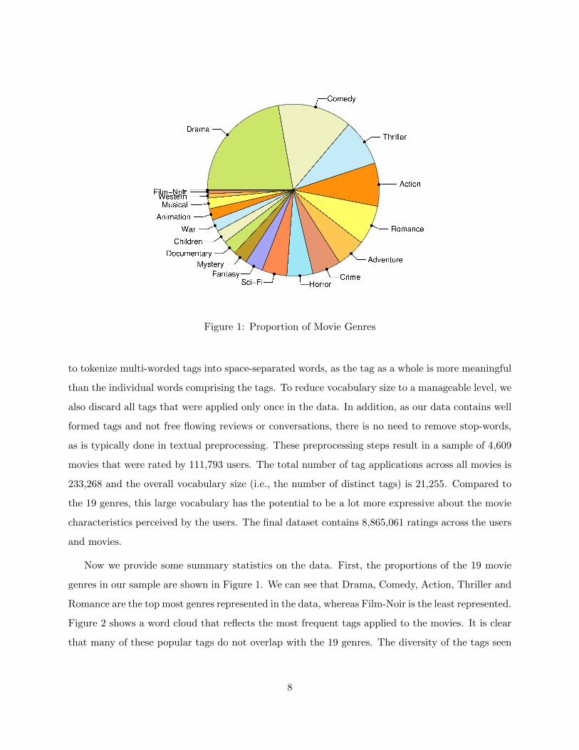
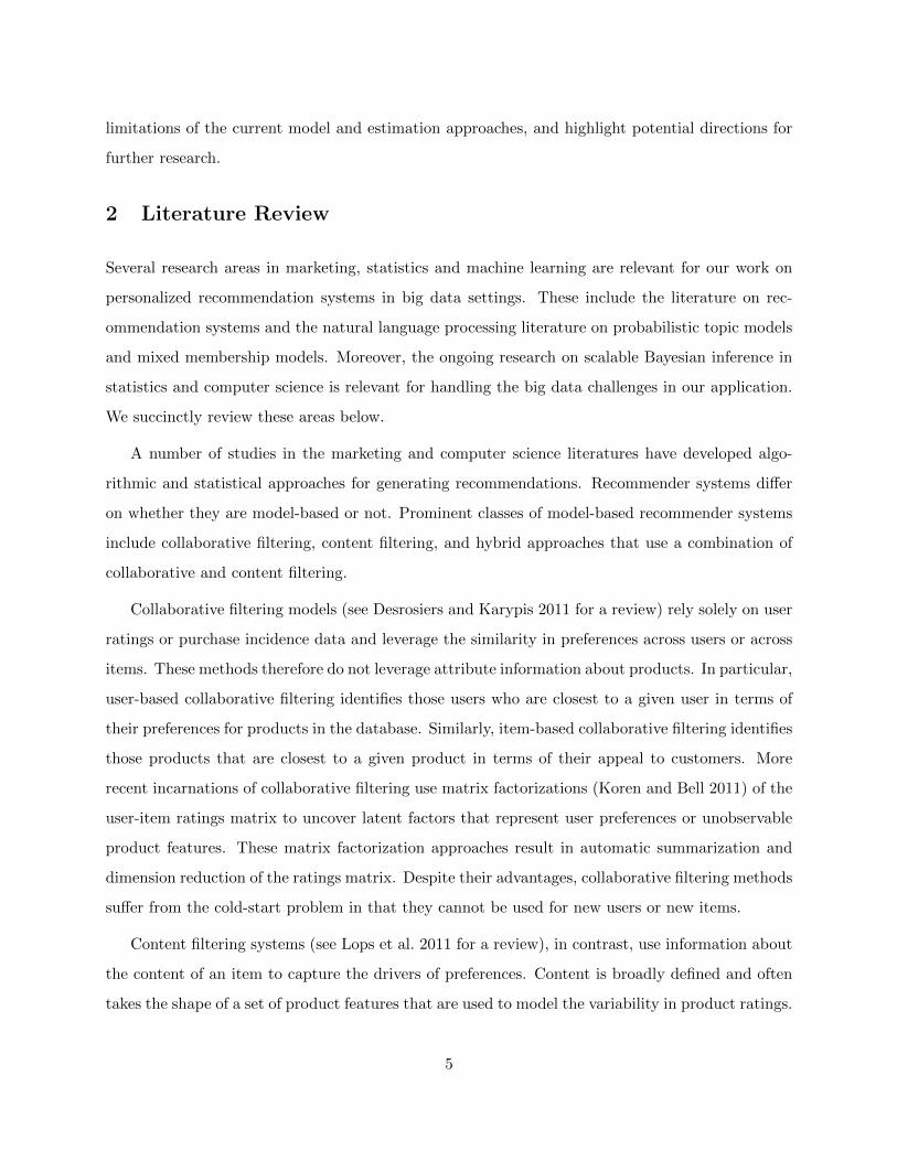
Figure 1: Proportion of Movie Genres
to tokenize multi-worded tags into space-separated words, as the tag as a whole is more meaningful
than the individual words comprising the tags. To reduce vocabulary size to a manageable level, we
also discard all tags that were applied only once in the data. In addition, as our data contains well
formed tags and not free flowing reviews or conversations, there is no need to remove stop-words,
as is typically done in textual preprocessing. These preprocessing steps result in a sample of 4,609
movies that were rated by 111,793 users. The total number of tag applications across all movies is
233,268 and the overall vocabulary size (i.e., the number of distinct tags) is 21,255. Compared to
the 19 genres, this large vocabulary has the potential to be a lot more expressive about the movie
characteristics perceived by the users. The final dataset contains 8,865,061 ratings across the users
and movies.
Now we provide some summary statistics on the data. First, the proportions of the 19 movie
genres in our sample are shown in Figure 1. We can see that Drama, Comedy, Action, Thriller and
Romance are the top most genres represented in the data, whereas Film-Noir is the least represented.
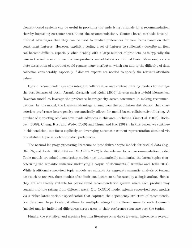
Figure 2 shows a word cloud that reflects the most frequent tags applied to the movies. It is clear
that many of these popular tags do not overlap with the 19 genres. The diversity of the tags seen
8

Figure 2: Word Cloud of Movie Tags
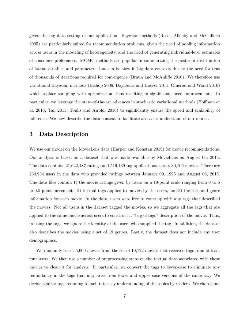
Figure 3: Histogram of the Number of Tags Received by Each Movie
in the word cloud highlights the importance of using crowd-sourced tagging to generate content
attributes beyond traditional standard attributes for describing and recommending products.
Figure 3 provides the histogram of the number of tags received by each movie. The median
number of tags for a movie is 16, with a mean of 50 and a standard deviation of 114.9. It is
interesting to note that the median number of tags is lower than 19, the number of pre-specified
genres within the data. The number of tags that were attached to a movie depends upon the movie’s
popularity and upon the time span for which it was part of the recommender system database.
9

(a) (b)
Figure 4: Scatter Plots for: (a) the Means and Standard Deviations of Ratings at Movie Level; (a)the Means and Standard Deviations of Ratings at User Level
As for the ratings, the mean across all observations of our data is 3.57, with a standard deviation
of 1.03, and the median rating is 4. There is considerable heterogeneity in the number of movies
that individuals rated. The median number of movies that a user rated is 43, and the mean is 79.
In addition, we compute the mean and standard deviation of the ratings received by each movie,
and similarly the mean and standard deviation of the ratings supplied by each individual. Figure
4 shows the scatter plots of these statistics. It is clear from the figures that there is considerable
heterogeneity in the ratings at both the movie and the user levels. The negative correlation that is
evident in both plots implies that the movies with lower mean ratings also exhibit higher variability
in their ratings and similarly, users who on average give low ratings also have higher variability in
their ratings. These observations make sense as movies that are not universally loved or hated (i.e.
cult movies) would appeal differently to different users. Users who tend to be more critical would
analyze the films more carefully, thus giving more nuanced opinions.
4 Model
Our recommendation model applies to a database of standard attributes, textual descriptions and
user ratings for products. We index the products (or documents) by d ∈ {1, . . . , D} and the users
who rate these products by i ∈ {1, . . . , I}. Besides standard product attributes xd, each product
is also described by a textual description, which can be a “bag of words” agglomeration of reviews
10

for a product, or composed from product tags provided by customers. In our application this bag-
of-words is a collection of user-generated tags that describe the features/aspects of the product.
A given product description can include multiple instances of the same tag, as the frequency with
which a given tag occurs within a product description depends upon how many people think the
tag is a relevant descriptor for the product. It is important to note that our use of bag-of-words
description is not restrictive, in that there is no inherent sequential ordering to the tag applications,
unlike in natural text (e.g., reviews) where the semantic meaning of the text depends critically on
the sequence of words in a sentence and in a paragraph.
The textual description associated with product d can be represented by a vector wd =
{wd1, wd2, . . . , wdNd}, where wdn represents the n-th token, or tag application within wd. The
set of unique tags across all product descriptions is indexed by v ∈ {1, . . . , V }, where V is the
vocabulary size, i.e., the total number of unique tags within the database. In addition to the prod-
uct content, the database also contains product ratings {yid} provided by the users as part of the
normal operations of the recommender system. The matrix of product ratings is sparse, as only a
fraction of all products are rated by a given user and a fraction of all users provide ratings to a
given product.
We assume that the information in the textual description for each product can be summa-
rized using a set of k = 1, . . . ,K topics. A topic can be considered as a discrete probability
distribution over the vocabulary. Topic k, therefore, is characterized by the probability vector
τ k = {τk1, . . . , τkV }, where the element τkv indicates the probability with which the tag v occurs
under topic k. The probability vector τ k is assumed to come from a symmetric Dirichlet distribution
Dir(τ k|η), where η > 0 is a scalar concentration parameter. The symmetric Dirichlet distribution
is a special case of Dirichlet distribution where all the elements of the Dirichlet parameter vector
are assumed to be equal. Applying symmetric Dirichlet is appropriate for topic distributions as we
do not possess prior knowledge that favors one token over another.
The K topics differ in the probabilities τkv with which they generate a given tag v. All the
products in a given recommender system share the same set of topics, but each product description
exhibits a mix of topics that is unique to itself, thus yielding a mixed-membership model (Ershoeva,
Blei and Lafferty 2009). The probability with which the K topics are represented within a product
description d are given by the vector of topic proportions ωd = {ωd1, . . . , ωdK}. This vector varies
11
across the products according to another Dirichlet distribution Dir(ωd|αd), where the Dirichlet
parameter αd is product specific and follows a log-normal distribution, i.e., αd ∼ logN (xdν, δ2).
In the MovieLens data, the standard product attributes include the pre-specified 19 movie genres,
each of which is represented as a binary variable. A movie can exhibit multiple genres and a vector
xd of binary variables for each movie. In this way, we allow the standard product attributes such as
movie genres to influence the topic mix in a user-generated product description, and the estimates
of ν and δ2 will indicate the average and variability of such influence.
We also assume that the rating yid that user i gives to product d reflects the user’s preferences
for the product. These ratings can be explained in terms of a parameter vector γi for user i. The
coefficients in γi reflect the extent to which the different latent semantic dimensions (i.e., topics)
matter in explaining the ratings. We assume that the users differ in the preference vectors and
model the heterogeneity in preferences via a normal population distribution, γi ∼ N (β,Γ), where β
represents the population mean and Γ represents the population covariance matrix. The diagonal
elements of the covariance matrix captures the variability in the preference parameters and its
off-diagonal elements reflect how the preferences for different latent topics covary across users.
We fuse together the cross-nested tag applications and ratings to jointly uncover the latent
topics that best predict the product ratings and the preference parameters that underlie these
ratings. As the data contains multiple ratings from each user, we are able to properly account
for sources of unobserved user heterogeneity, which is critical for capturing user preferences in
terms of the latent topics. Given the above description, our model can be specified using the
following generative process. Fixing the number of topicsK, the Dirichlet parameter η, the Dirichlet
regression parameters ν and δ2, the population parameters β and Γ, and the error variance σ2, the
CGSTM model generates product descriptions and their associated ratings as follows:
1. Draw topic distribution for each topic, τ k ∼ Dir(η).
2. Draw the Dirichlet parameter αd for each product, αd ∼ logN (xdν, δ2).
3. Draw topic proportions for each product, ωd ∼ Dir(αd).
4. For each tag application n belonging to product description d,
a) Draw topic zdn ∼ Multinomial(ωd).
12

, Γ
Figure 5: Directed Acyclic Graph for The Cross-Nested Topic Model
b) Draw tag wdn ∼ Multinomial(τ zdn).
5. For each user i who rated product d,
a) Draw his/her preference parameters γi ∼ N (β,Γ).
b) Draw the rating yid ∼ N (z′dγi, σ2), where zd = (1/Nd)
∑Ndn=1 zdn.
Figure 5 shows the directed acyclic graph for the CGSTM model. The model structure differs
from the hybrid models in the recommender system literature in that the content variables are
specified through the unobserved empirical frequencies of the latent topics within each product
description. By relating the ratings to the mean unobserved frequencies zd, rather than on the
topic proportions ωd, we ensure that the ratings are determined by the topic frequencies that
actually underlie the bag of tags description of the product. Such an approach is likely to yield
latent topics that not only capture the semantic content of the tags, but are also most predictive of
the user ratings and reflective of the standard product attributes. Therefore, this approach has the
potential to improve the predictive ability of the model – the central objective of most recommender
systems.
13
5 Posterior Inference via Stochastic Variational Bayes
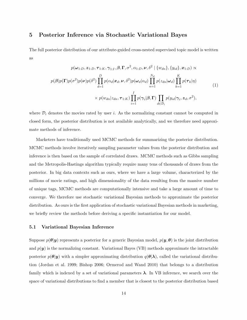
The full posterior distribution of our attribute-guided cross-nested supervised topic model is written
as
p(ω1:D, z1:D, τ 1:K ,γ1:I ,β,Γ, σ2, α1:D,ν, δ
2 | {wdn}, {yid},x1:D) ∝
p(β)p(Γ)p(σ2)p(ν)p(δ2)D∏d=1
p(αd|xd,ν, δ2)p(ωd|αd)Nd∏n=1
p(zdn|ωd)K∏k=1
p(τ k|η)
× p(wdn|zdn, τ 1:K)I∏i=1
p(γi|β,Γ)∏d∈Di
p(yid|γi, zd, σ2),
(1)
where Di denotes the movies rated by user i. As the normalizing constant cannot be computed in
closed form, the posterior distribution is not available analytically, and we therefore need approxi-
mate methods of inference.
Marketers have traditionally used MCMC methods for summarizing the posterior distribution.
MCMC methods involve iteratively sampling parameter values from the posterior distribution and
inference is then based on the sample of correlated draws. MCMC methods such as Gibbs sampling
and the Metropolis-Hastings algorithm typically require many tens of thousands of draws from the
posterior. In big data contexts such as ours, where we have a large volume, characterized by the
millions of movie ratings, and high dimensionality of the data resulting from the massive number
of unique tags, MCMC methods are computationally intensive and take a large amount of time to
converge. We therefore use stochastic variational Bayesian methods to approximate the posterior
distribution. As ours is the first application of stochastic variational Bayesian methods in marketing,
we briefly review the methods before deriving a specific instantiation for our model.
5.1 Variational Bayesian Inference
Suppose p(θ|y) represents a posterior for a generic Bayesian model, p(y,θ) is the joint distribution
and p(y) is the normalizing constant. Variational Bayes (VB) methods approximate the intractable
posterior p(θ|y) with a simpler approximating distribution q(θ|λ), called the variational distribu-
tion (Jordan et al. 1999; Bishop 2006; Ormerod and Wand 2010) that belongs to a distribution
family which is indexed by a set of variational parameters λ. In VB inference, we search over the
space of variational distributions to find a member that is closest to the posterior distribution based
14
on the Kullback-Leibler (KL) divergence (Kullback and Leibler 1951).
5.1.1 Kullback-Leibler Divergence and ELBO
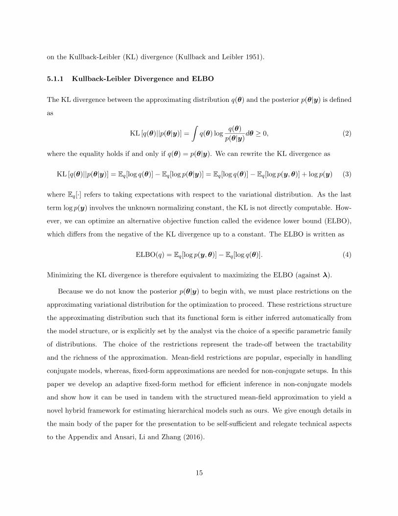
The KL divergence between the approximating distribution q(θ) and the posterior p(θ|y) is defined
as
KL [q(θ)||p(θ|y)] =
∫q(θ) log
q(θ)
p(θ|y)dθ ≥ 0, (2)
where the equality holds if and only if q(θ) = p(θ|y). We can rewrite the KL divergence as
KL [q(θ)||p(θ|y)] = Eq[log q(θ)]− Eq[log p(θ|y)] = Eq[log q(θ)]− Eq[log p(y,θ)] + log p(y) (3)
where Eq[·] refers to taking expectations with respect to the variational distribution. As the last
term log p(y) involves the unknown normalizing constant, the KL is not directly computable. How-
ever, we can optimize an alternative objective function called the evidence lower bound (ELBO),
which differs from the negative of the KL divergence up to a constant. The ELBO is written as
ELBO(q) = Eq[log p(y,θ)]− Eq[log q(θ)]. (4)
Minimizing the KL divergence is therefore equivalent to maximizing the ELBO (against λ).
Because we do not know the posterior p(θ|y) to begin with, we must place restrictions on the
approximating variational distribution for the optimization to proceed. These restrictions structure
the approximating distribution such that its functional form is either inferred automatically from
the model structure, or is explicitly set by the analyst via the choice of a specific parametric family
of distributions. The choice of the restrictions represent the trade-off between the tractability
and the richness of the approximation. Mean-field restrictions are popular, especially in handling
conjugate models, whereas, fixed-form approximations are needed for non-conjugate setups. In this
paper we develop an adaptive fixed-form method for efficient inference in non-conjugate models
and show how it can be used in tandem with the structured mean-field approximation to yield a
novel hybrid framework for estimating hierarchical models such as ours. We give enough details in
the main body of the paper for the presentation to be self-sufficient and relegate technical aspects
to the Appendix and Ansari, Li and Zhang (2016).
15
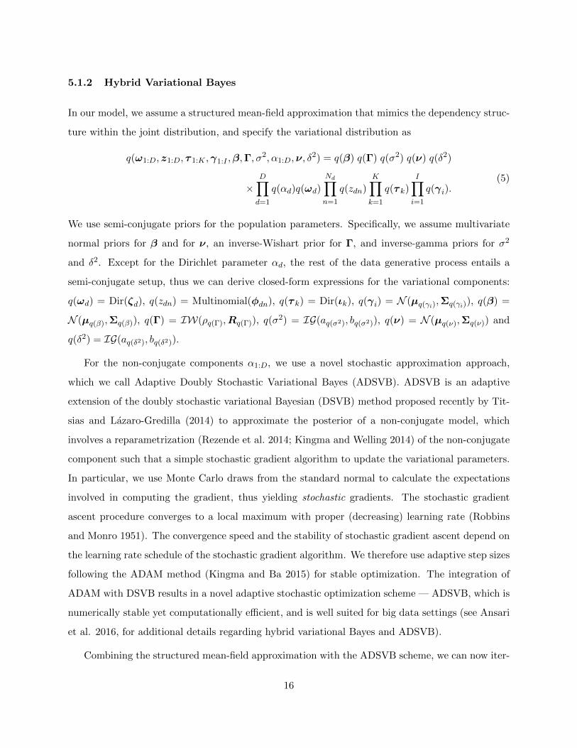
5.1.2 Hybrid Variational Bayes
In our model, we assume a structured mean-field approximation that mimics the dependency struc-
ture within the joint distribution, and specify the variational distribution as
q(ω1:D, z1:D, τ 1:K ,γ1:I ,β,Γ, σ2, α1:D,ν, δ
2) = q(β) q(Γ) q(σ2) q(ν) q(δ2)
×D∏d=1
q(αd)q(ωd)
Nd∏n=1
q(zdn)K∏k=1
q(τ k)I∏i=1
q(γi).(5)
We use semi-conjugate priors for the population parameters. Specifically, we assume multivariate
normal priors for β and for ν, an inverse-Wishart prior for Γ, and inverse-gamma priors for σ2
and δ2. Except for the Dirichlet parameter αd, the rest of the data generative process entails a
semi-conjugate setup, thus we can derive closed-form expressions for the variational components:
q(ωd) = Dir(ζd), q(zdn) = Multinomial(φdn), q(τ k) = Dir(ιk), q(γi) = N (µq(γi),Σq(γi)), q(β) =
N (µq(β),Σq(β)), q(Γ) = IW(ρq(Γ),Rq(Γ)), q(σ2) = IG(aq(σ2), bq(σ2)), q(ν) = N (µq(ν),Σq(ν)) and
q(δ2) = IG(aq(δ2), bq(δ2)).
For the non-conjugate components α1:D, we use a novel stochastic approximation approach,
which we call Adaptive Doubly Stochastic Variational Bayes (ADSVB). ADSVB is an adaptive
extension of the doubly stochastic variational Bayesian (DSVB) method proposed recently by Tit-
sias and Lazaro-Gredilla (2014) to approximate the posterior of a non-conjugate model, which
involves a reparametrization (Rezende et al. 2014; Kingma and Welling 2014) of the non-conjugate
component such that a simple stochastic gradient algorithm to update the variational parameters.
In particular, we use Monte Carlo draws from the standard normal to calculate the expectations
involved in computing the gradient, thus yielding stochastic gradients. The stochastic gradient
ascent procedure converges to a local maximum with proper (decreasing) learning rate (Robbins
and Monro 1951). The convergence speed and the stability of stochastic gradient ascent depend on
the learning rate schedule of the stochastic gradient algorithm. We therefore use adaptive step sizes
following the ADAM method (Kingma and Ba 2015) for stable optimization. The integration of
ADAM with DSVB results in a novel adaptive stochastic optimization scheme — ADSVB, which is
numerically stable yet computationally efficient, and is well suited for big data settings (see Ansari
et al. 2016, for additional details regarding hybrid variational Bayes and ADSVB).
Combining the structured mean-field approximation with the ADSVB scheme, we can now iter-
16
atively update the variational parameters via coordinate ascent. The resulting estimation process
involve using ADSVB to update α1:D, which serves as an inner loop within an outer loop that
updates for all other (conjugate) parameters using coordinate ascent. To speed up inference in the
big data setting, next we develop a stochastic variational Bayesian procedure.
5.2 Speeding Up Variational Bayes
When fitting a complex model with many individual level latent parameters to a big data set,
the coordinate-ascent procedure requires significant computation because of the need to iteratively
update each latent variable. In particular, we need to update the latent variables associated with
each user in each iteration. This becomes a computational bottleneck if the data contains a large
number of individuals. Recent research has explored strategies to speed up this computation via
stochastic variational inference (Hoffman et al. 2013).
5.2.1 Stochastic Optimization with Adaptive Mini-batch
Recall that in variational Bayesian estimation, our goal is to maximize the ELBO defined in (4).
In the proposed CGSTM model, the ELBO for movie d has the form:
ELBOd = E[log p(ωd|αd)] +
Nd∑n=1
E[log p(zdn|ωd)] +
Nd∑n=1
E[log p(wdn|zdn, τ 1:K)]
+
Id∑i=1
E[log p(yid)|zd,γi, σ2] +
Id∑i=1
E[log p(γi|β,Γ)] +
K∑k=1
E[log p(τ k|η)] +H(q),
(6)
where the expectation is taken with respect to the corresponding variational distributions, Iddenotes the number of individuals who rated movie d, and the last term H(q) is the entropy over
the entire set of variational distributions in the model. In each iteration of optimizing ELBO, we
take the gradient of the objective function, from which we move the ELBO towards the direction of
the steepest ascent. In the computation, in every iteration we need to go through each individual
to update their specific coefficients and then form the gradient of the ELBO. When there are a
massive number of individuals in the data, a typical big data situation in marketing, this process
substantially slows down the computation. Given that the ELBO and its gradient both involve
a sum of individual terms that are independent conditional on the population level parameters,
the theory on stochastic optimization (Robins and Monro 1951; Spall 2003) allows us to save on
17
computation by only going through a random subsample of individuals in each iteration to obtain
a noisy gradient to update the objective. Because such a cheaply computed gradient is unbiased
across iterations, the objective function will probabilistically converge to an optimum under proper
regulatory conditions (Hoffman et al. 2013).
Specifically, in iteration t, we randomly sample a subset of individuals (without replacement) —
a mini-batch of the data, S(t), and update only the γi’s corresponding to these individuals. Based
on the updated individual parameters we then construct a stochastic gradient to update the other
parameters at the population level (invariant across individuals) in (6). Because the optimization
process is recursive, i.e., updating one parameter depends on the current values of all other parame-
ters, the updating of the individual parameters in the mini-batch is also a function of the population
parameters. At the early iterations, the population parameters are still far from optimality, so it
is wasteful to take large mini-batch because updating the individual parameters in the mini-batch
has low precision anyway, due to the unconverged population parameters. In fact, we can further
save on computation by sampling smaller mini-batch (i.e., fewer individuals) at the beginning of
the optimization process. From that we quickly and stochastically move the estimation towards
the proper direction, and increase the size of the mini-batch (i.e., sampling more individuals) in
later iterations only if more precision is needed for converging on an optimum. Essentially, we have
an adaptive procedure that automatically determines the most appropriate batch size to use in a
given iteration, leading to significant improvement in the speed and scalability of the already fast
variational Bayesian estimation. In this strategy, it is important to have a rule on when and how
to increase mini-batch size during the process. In current paper we adopt the “ratio of path and
progress” criterion (RPP; Gaivoronski 1988; Tan 2015) and let the estimation procedure determine
by itself when to sample more individuals into the mini-batch and by how many. Appendix A
provides the necessary technical details for implementing this adaptation strategy for stochastic
VB. Appendix B outlines the full procedure of stochastic variational Bayesian estimation for the
main model.
18
6 Results
6.1 Null Models and Holdout Data
We compare our cross-nested topic model to a hierarchical Bayesian model that uses the pre-
specified 19 genres as covariates. As each movie is represented in terms of multiple genres, we
have a set of 19 genre-specific coefficients and an intercept for each user. We assume that the
individual level coefficients come from a multivariate normal population distribution with a full
covariance structure. A comparison between the null and the proposed models can help us assess
the predictive benefits that arise from the greater expressive power of the crowd-sourced semantic
representations inherent in the latent topics. We estimate both models using stochastic variational
Bayesian methods. With a convergence criterion of 10−6 on the ELBO, the variational Bayesian
estimation on the null model finishes at 10 iterations with 585.9 seconds (0.16 hours), whereas the
MCMC estimation of the same model with 5000 runs takes 21.1 hours to complete1. Also, the
(mean) parameter estimates between VB and MCMC are virtually indistinguishable2. Given the
SVB significantly outperforms MCMC in computational time, when estimating the main model
that is far more complex than the null, we do not use MCMC because we expect that MCMC
methods will not be competitive in terms of the computational time needed for estimation. Our
model contains a very large number of latent variables, including the multinomial topic indicators
for each of the 233,268 tag applications, and multivariate user-level coefficients for each of the
111,793 users. The use of data augmentation to sample these latent variables is likely to be time
consuming, especially given that MCMC typically takes a much larger number of iterations to
converge, when compared to VB.
To evaluate the predictive performance of the genre-only model and the CGSTM model, we
split our dataset into calibration and holdout samples. We estimate both models on the calibration
data and make predictions on both datasets. To form the holdout data, we set aside 8 movies per
individual. This resulted in a total of 7,970,717 ratings in the calibration data and 894,344 ratings
in the holdout data. The movies and users in either dataset are the same as in the full sample.
1For a fair comparison we code both VB and MCMC in Mathematica 10 and use the just-in-time compilationcapability of Mathematica to compile the programs to C. We run both programs on a computer with 3GHz 8-CoreIntel Xeon E5 processor and 32G of RAM.
2The underestimation of parameter uncertainty is still present under the mean-field VB estimation, albeit the useof structured mean-field that mitigates such effect. However, for the purposes of model prediction and the productrecommendation, it is the mean estimates of model parameters that matter.
19
We estimate multiple versions of the proposed model that differ on the number of topics K.
Based on model fit and predictive performance reported below, we settle on a model with 20
topics and the results presented here are all obtained from this version. We estimate our model
using both deterministic and stochastic variational Bayesian methods. The deterministic VB takes
18,930 seconds (5.3 hours) and 275 iterations to converge, whereas the stochastic VB with adaptive
mini-batch sizes takes only 4,667 seconds (1.3 hours) and 150 iterations to finish. Convergence is
declared when the joint Euclidean norm on the population level parameters changes by less than
10−4 between iterations. The substantial difference in computational times once again highlights
the scalability benefits of stochastic variational inference in big data settings. Details of our SVB
approach are outlined in Appendix B. As the actual estimates do not vary across the two estimation
schemes, we now report the results from the SVB approach. We begin with the qualitative insights
that can be gleaned from our model and discuss predictive performance and model fit subsequently.
6.2 Recovery of Topics
Topic Distributions The model yields topic distributions that are most predictive of the ratings.
Table 1 shows the top 8 tags within each of the 20 topics. These topics are arranged in ascending
order of the population mean coefficients β on the topics. Thus the most important topics are
shown at the bottom of Table 1. It is interesting to see how certain tags naturally congregate
to form meaningful topics. For example, Topic 18 is about American animation movies, often
produced by Pixar and Disney, for children and are usually fairy-tales and romance-themed. Topic
12 is about Japanese animation movies, which is predominantly made by Mr. Miyazaki of Studio
Ghibli, whose style is quite different from those of the “family-fun” Disney or Pixar productions.
His films tend to have story lines and characters that are fantastic, surreal and dream-like in nature
(e.g. Spirited Away, Howl’s Moving Castle, to name a few), perhaps even eliciting feelings of drug-
induced “hallucination” for certain users. Topic 10 appears to be closely related to the director
Quentin Tarantino, who uses action and violence as overarching styles in all of his firms, and has
directed works related to WWII (The Inglorious Bastards, starring Brad Pitt), martial art (Kill
Bill), and revenge (Kill Bill, Pulp Fiction). It is clear that the topics richly depict the semantic
information pertaining to the theme, provenance, popularity, awards, and actors of a movie. Thus
they capture a much greater semantic terrain than what is possible using a set of genre dummies.
20
Tab
le1:
Top
Eig
ht
Tag
sA
ssoci
ated
wit
hE
ach
Top
ic
Top
icT
op
8W
ord
sW
ith
inE
ach
Top
ic
1b
ase
don
ab
ook
nu
dit
y(t
op
less
)fr
an
chis
ere
make
nata
lie
port
man
act
ion
sequ
elst
up
id2
pre
dic
tab
leb
ori
ng
ad
am
san
dle
ract
ing
silly
plo
tst
ory
bad
plo
t3
sport
snu
dit
y(t
op
less
)b
d-r
bet
am
ax
boxin
gca
rsp
olice
sylv
este
r-st
allon
e4
zom
bie
sh
orr
or
dis
turb
ing
seri
al
kille
rcu
ltfi
lmgore
cree
py
cam
py
5jo
hn
ny
dep
pti
mb
urt
on
mu
sica
lb
ase
don
ab
ook
goth
icvis
ually
ap
pea
lin
ggh
ost
sad
ap
ted
:book
6atm
osp
her
iccr
iter
ion
nu
dit
y(f
ull
fronta
l)b
ase
don
ab
ook
dis
turb
ing
slow
stan
ley
ku
bri
ckm
enta
lilln
ess
7qu
irky
cin
emato
gra
phy
hig
hsc
hool
scarl
ett
joh
an
sson
rela
tion
ship
sco
min
gof
age
ph
ilip
hoff
man
suic
ide
8re
ligio
nle
ssth
an
300
rati
ngs
gay
chri
stia
nit
yle
sbia
nqu
eer
jesu
sb
riti
sh9
sup
erh
ero
act
ion
com
icb
ook
jam
esb
on
dm
arv
eln
ewyork
city
will
smit
hfr
an
chis
e10
qu
enti
nta
ranti
no
worl
dw
ar
iire
ven
ge
mart
ial
art
svio
len
ceb
rad
pit
tact
ion
wes
tern
11
politi
csso
cial
com
men
tary
docu
men
tary
tru
est
ory
mu
sici
an
sm
usi
ch
isto
ryco
rru
pti
on
12
an
ime
surr
eal
dru
gs
styli
zed
stu
dio
gh
ibli
jap
an
hayao
miy
aza
ki
hallu
cin
ato
ry13
thou
ght-
pro
vokin
gsu
rrea
lti
me
travel
sci-
fin
on
lin
ear
min
dfu
ckvis
ually
ap
pea
lin
gco
mp
lica
ted
14
com
edy
fun
ny
paro
dy
hilari
ou
sw
itty
sati
reb
ill
murr
ay
hig
hsc
hool
15
sci-
fid
yst
op
iaact
ion
space
post
-ap
oca
lyp
tic
alien
sart
ifici
al
inte
llig
ence
ad
ven
ture
16
twis
ten
din
gth
riller
base
don
ab
ook
myst
ery
psy
cholo
gic
al
psy
cholo
gy
chri
stia
nb
ale
morg
an
-fre
eman
17
class
icafi
bla
ckan
dw
hit
eb
d-r
clv
noir
thri
ller
osc
ar
(bes
tp
ictu
re)
esp
ion
age
18
fanta
syan
imati
on
pix
ar
dis
ney
ad
ven
ture
fair
yta
lero
man
cech
ild
ren
19
dra
ma
rom
an
ceb
ase
don
atr
ue
story
tom
han
ks
tru
est
ory
his
tori
cal
osc
ar
(bes
tp
ictu
re)
insp
irati
on
al
20
atm
osp
her
icd
ark
com
edy
stylize
dqu
irky
bla
ckco
med
yim
db
top
250
vio
len
cecu
ltfi
lm
Tab
le2:
Pop
ula
tion
Coeffi
cien
tsan
dV
aria
nce
sA
ssoci
ated
wit
hth
eT
opic
s
Topic
12
34
56
78
910
11
12
13
14
15
16
17
18
19
20
β1.0
22.4
12.8
12.9
93.1
63.2
53.3
53.4
83.5
33.5
43.5
93.6
33.6
63.6
93.9
94.1
04.1
44.1
84.2
24.5
9D
iag(Γ
)1.9
70.8
80.8
01.1
10.5
61.8
70.9
00.6
80.4
30.5
00.4
81.2
30.4
30.5
40.4
80.5
60.4
80.6
30.5
80.7
8
21
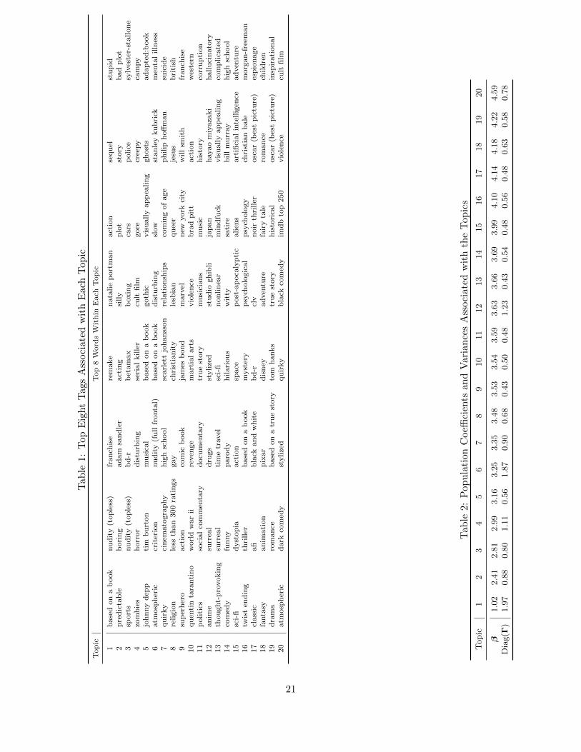
Table 2 reports the population mean coefficient and the population variance associated with each
topic. The table shows that movies associated with the last few topics tend to have high ratings,
on average. We also see that the heterogeneity associated with the individual level coefficients γi
varies across the topics. The large magnitude of these cross-user variances indicates that users
exhibit considerable heterogeneity in their sensitivities on different topics.
This result exhibits face validity as higher numbered topics tend to contain characteristics that
most users would consider to be desirable. For example, Topic 19 contains “Oscar”, “true story”
and “inspirational”, and Topic 20 includes “IMDB top 250” and semantics related to dark humor,
which often sets a high requirement for screenplay excellence. All of these qualities are considered
desirable by most people, thus resulting in higher mean and smaller standard deviation. On the
other hand, lower numbered topics tend to contain more negative and polarizing semantics. For
instance, for Topics 1 and 2, although there exist fans of silly, sequel, or Adam Sandler movies,
many others might consider them as undesirable, as evidenced by tags such as “predictable” and
“boring”.
Top Movies Associated with a Topic Apart from the above topic descriptions, we can also
identify the top movies associated with each topic using the topic proportions ωd for movies.
Specifically, for a given topic k, we find movies that have large values for the proportions ωdk. Due
to the limits stemming from page size, Table 3 shows only the top three movies associated with
each of the 20 topics.
It can be seen by juxtaposing Tables 1 and 3 that the identified top movies are consistent with
the semantic content of the topic. For example, the top movies associated with Topic 9 include
different sequels of “Iron Man” and “Spider-Man”, which is highly consistent with the top 8 tags
for that topic in Table 1 that describes the topic as films based on action super heroes from the
franchise Marvel Comics. Another example of top movies that emerge from the model is under Topic
19, which include dramas based on inspirational historical backgrounds that have won Oscars (i.e.
Forrest Gump, Titanic and The King’s Speech). Movie enthusiasts would also note that, although
the top movies associated with Topic 20 are also critically acclaimed, they are of a different flavor
compared to those of Topic 19. For example, Black Swan, Pulp Fiction and Wristcutters’ successes
22
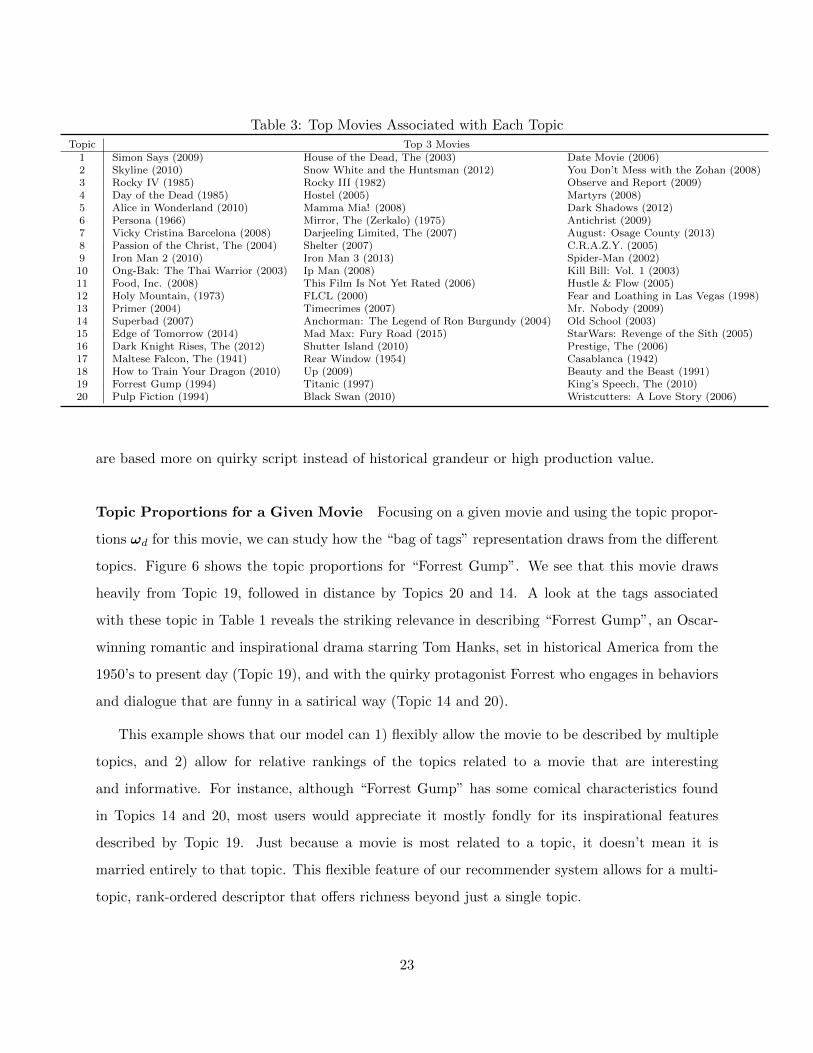
Table 3: Top Movies Associated with Each Topic
Topic Top 3 Movies1 Simon Says (2009) House of the Dead, The (2003) Date Movie (2006)2 Skyline (2010) Snow White and the Huntsman (2012) You Don’t Mess with the Zohan (2008)3 Rocky IV (1985) Rocky III (1982) Observe and Report (2009)4 Day of the Dead (1985) Hostel (2005) Martyrs (2008)5 Alice in Wonderland (2010) Mamma Mia! (2008) Dark Shadows (2012)6 Persona (1966) Mirror, The (Zerkalo) (1975) Antichrist (2009)7 Vicky Cristina Barcelona (2008) Darjeeling Limited, The (2007) August: Osage County (2013)8 Passion of the Christ, The (2004) Shelter (2007) C.R.A.Z.Y. (2005)9 Iron Man 2 (2010) Iron Man 3 (2013) Spider-Man (2002)10 Ong-Bak: The Thai Warrior (2003) Ip Man (2008) Kill Bill: Vol. 1 (2003)11 Food, Inc. (2008) This Film Is Not Yet Rated (2006) Hustle & Flow (2005)12 Holy Mountain, (1973) FLCL (2000) Fear and Loathing in Las Vegas (1998)13 Primer (2004) Timecrimes (2007) Mr. Nobody (2009)14 Superbad (2007) Anchorman: The Legend of Ron Burgundy (2004) Old School (2003)15 Edge of Tomorrow (2014) Mad Max: Fury Road (2015) StarWars: Revenge of the Sith (2005)16 Dark Knight Rises, The (2012) Shutter Island (2010) Prestige, The (2006)17 Maltese Falcon, The (1941) Rear Window (1954) Casablanca (1942)18 How to Train Your Dragon (2010) Up (2009) Beauty and the Beast (1991)19 Forrest Gump (1994) Titanic (1997) King’s Speech, The (2010)20 Pulp Fiction (1994) Black Swan (2010) Wristcutters: A Love Story (2006)
are based more on quirky script instead of historical grandeur or high production value.
Topic Proportions for a Given Movie Focusing on a given movie and using the topic propor-
tions ωd for this movie, we can study how the “bag of tags” representation draws from the different
topics. Figure 6 shows the topic proportions for “Forrest Gump”. We see that this movie draws
heavily from Topic 19, followed in distance by Topics 20 and 14. A look at the tags associated
with these topic in Table 1 reveals the striking relevance in describing “Forrest Gump”, an Oscar-
winning romantic and inspirational drama starring Tom Hanks, set in historical America from the
1950’s to present day (Topic 19), and with the quirky protagonist Forrest who engages in behaviors
and dialogue that are funny in a satirical way (Topic 14 and 20).
This example shows that our model can 1) flexibly allow the movie to be described by multiple
topics, and 2) allow for relative rankings of the topics related to a movie that are interesting
and informative. For instance, although “Forrest Gump” has some comical characteristics found
in Topics 14 and 20, most users would appreciate it mostly fondly for its inspirational features
described by Topic 19. Just because a movie is most related to a topic, it doesn’t mean it is
married entirely to that topic. This flexible feature of our recommender system allows for a multi-
topic, rank-ordered descriptor that offers richness beyond just a single topic.
23

Figure 6: Topic Proportions for Forrest Gump
We see from the above that our model is capable of generating deep qualitative insights about
the underlying drivers for movie preference. Such information is highly valuable in a recommender
system as it can be used to explain why a particular product is being recommended. We now move
on to show how the model can be used for recommending products to users and how it does in
predicting preferences. We begin by showing how our model can be used to identify movies that
are similar to a given movie.
Movies Similar to a Given Movie Item-based collaborative filtering algorithms identify those
products that are closest to a given product in their appeal to customers. This is usually done
using solely the ratings matrix, and therefore, this approach suffers from the inability to explain
fully why a particular recommendation is being made.
Our model can be leveraged to compute distances between movies based on their topic pro-
portion vectors. While many different distance metrics can be used for this task, here we use the
Hellinger distance (Nikulin 2001) to compute the similarity between two movies, d and d′, based
on their topic proportions, ωd and ωd′ , respectively. The Hellinger distance is defined as
H(d, d′) =
√√√√1
2
K∑k=1
(√ωdk −
√ωd′k)2, (7)
and satisfies the triangle inequality. The use of the topic proportion vectors implies that both ratings
as well as textual content are utilized in computing closeness between movies, given that the topic
distribution is inferred taking into account both the tag and the rating information. Therefore this
is different from solely relying on movie ratings or on the content of movies in computing similarity.
24
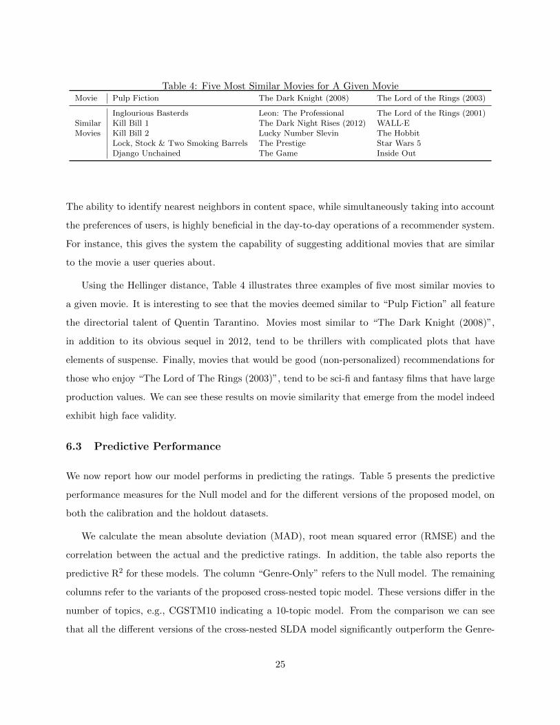
Table 4: Five Most Similar Movies for A Given MovieMovie Pulp Fiction The Dark Knight (2008) The Lord of the Rings (2003)
Inglourious Basterds Leon: The Professional The Lord of the Rings (2001)Similar Kill Bill 1 The Dark Night Rises (2012) WALL·EMovies Kill Bill 2 Lucky Number Slevin The Hobbit
Lock, Stock & Two Smoking Barrels The Prestige Star Wars 5Django Unchained The Game Inside Out
The ability to identify nearest neighbors in content space, while simultaneously taking into account
the preferences of users, is highly beneficial in the day-to-day operations of a recommender system.
For instance, this gives the system the capability of suggesting additional movies that are similar
to the movie a user queries about.
Using the Hellinger distance, Table 4 illustrates three examples of five most similar movies to
a given movie. It is interesting to see that the movies deemed similar to “Pulp Fiction” all feature
the directorial talent of Quentin Tarantino. Movies most similar to “The Dark Knight (2008)”,
in addition to its obvious sequel in 2012, tend to be thrillers with complicated plots that have
elements of suspense. Finally, movies that would be good (non-personalized) recommendations for
those who enjoy “The Lord of The Rings (2003)”, tend to be sci-fi and fantasy films that have large
production values. We can see these results on movie similarity that emerge from the model indeed
exhibit high face validity.
6.3 Predictive Performance
We now report how our model performs in predicting the ratings. Table 5 presents the predictive
performance measures for the Null model and for the different versions of the proposed model, on
both the calibration and the holdout datasets.
We calculate the mean absolute deviation (MAD), root mean squared error (RMSE) and the
correlation between the actual and the predictive ratings. In addition, the table also reports the
predictive R2 for these models. The column “Genre-Only” refers to the Null model. The remaining
columns refer to the variants of the proposed cross-nested topic model. These versions differ in the
number of topics, e.g., CGSTM10 indicating a 10-topic model. From the comparison we can see
that all the different versions of the cross-nested SLDA model significantly outperform the Genre-
25
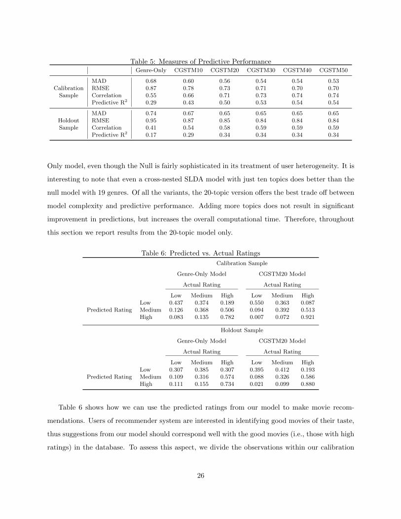
Table 5: Measures of Predictive PerformanceGenre-Only CGSTM10 CGSTM20 CGSTM30 CGSTM40 CGSTM50
MAD 0.68 0.60 0.56 0.54 0.54 0.53Calibration RMSE 0.87 0.78 0.73 0.71 0.70 0.70
Sample Correlation 0.55 0.66 0.71 0.73 0.74 0.74Predictive R2 0.29 0.43 0.50 0.53 0.54 0.54
MAD 0.74 0.67 0.65 0.65 0.65 0.65Holdout RMSE 0.95 0.87 0.85 0.84 0.84 0.84Sample Correlation 0.41 0.54 0.58 0.59 0.59 0.59
Predictive R2 0.17 0.29 0.34 0.34 0.34 0.34
Only model, even though the Null is fairly sophisticated in its treatment of user heterogeneity. It is
interesting to note that even a cross-nested SLDA model with just ten topics does better than the
null model with 19 genres. Of all the variants, the 20-topic version offers the best trade off between
model complexity and predictive performance. Adding more topics does not result in significant
improvement in predictions, but increases the overall computational time. Therefore, throughout
this section we report results from the 20-topic model only.
Table 6: Predicted vs. Actual Ratings
Calibration Sample
Genre-Only Model CGSTM20 Model
Actual Rating Actual Rating
Low Medium High Low Medium HighLow 0.437 0.374 0.189 0.550 0.363 0.087
Predicted Rating Medium 0.126 0.368 0.506 0.094 0.392 0.513High 0.083 0.135 0.782 0.007 0.072 0.921
Holdout Sample
Genre-Only Model CGSTM20 Model
Actual Rating Actual Rating
Low Medium High Low Medium HighLow 0.307 0.385 0.307 0.395 0.412 0.193
Predicted Rating Medium 0.109 0.316 0.574 0.088 0.326 0.586High 0.111 0.155 0.734 0.021 0.099 0.880
Table 6 shows how we can use the predicted ratings from our model to make movie recom-
mendations. Users of recommender system are interested in identifying good movies of their taste,
thus suggestions from our model should correspond well with the good movies (i.e., those with high
ratings) in the database. To assess this aspect, we divide the observations within our calibration
26
and holdout samples into three groups (i.e., Low, Medium and High) based on the 1/3 and 2/3
percentiles of the predicted ratings. We then compute the proportions of observations within each
of these three groups that have Low (actual ratings from zero to 2), Medium (actual ratings from
2.5 to 3.5), and High (actual rating from 4 to 5) ratings. For example, for the CGSTM20 model,
the entry 0.921 of the High-High cell for the calibration sample indicates that 92.1% of the obser-
vations that the model predicts to have high ratings indeed have true ratings between 4 and 5. It is
clear from the table that our proposed model predicts much better than the “Genre-Only” model
in each of the three groups, on both the calibration and the holdout samples. We also see that the
predictions in the holdout sample are slightly worse than the calibration sample, as expected.
6.4 Movie Recommendations
We now focus on how our model can be used in different ways for recommending movies to users.
We first show how we can make unconditional recommendations for a given user. We then show
how the model also supports personalized search based on user queries. We also provide a succinct
interpretation of these recommendations.
6.4.1 Unconditional Recommendations without User Query
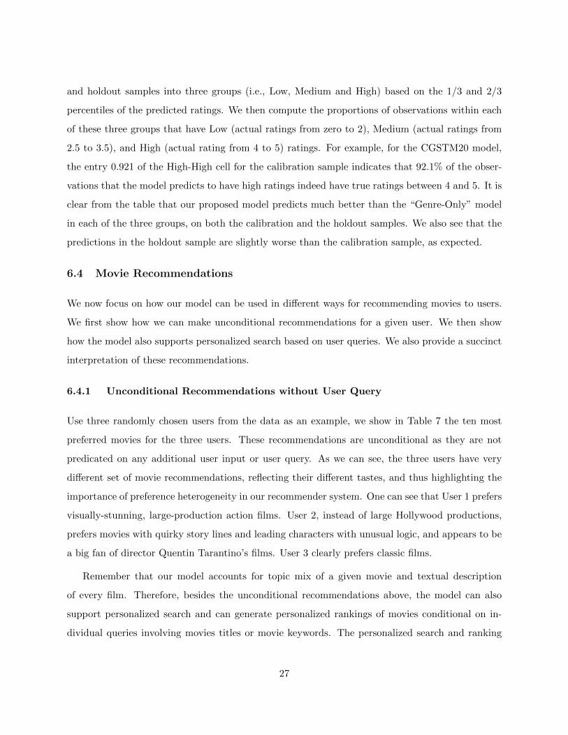
Use three randomly chosen users from the data as an example, we show in Table 7 the ten most
preferred movies for the three users. These recommendations are unconditional as they are not
predicated on any additional user input or user query. As we can see, the three users have very
different set of movie recommendations, reflecting their different tastes, and thus highlighting the
importance of preference heterogeneity in our recommender system. One can see that User 1 prefers
visually-stunning, large-production action films. User 2, instead of large Hollywood productions,
prefers movies with quirky story lines and leading characters with unusual logic, and appears to be
a big fan of director Quentin Tarantino’s films. User 3 clearly prefers classic films.
Remember that our model accounts for topic mix of a given movie and textual description
of every film. Therefore, besides the unconditional recommendations above, the model can also
support personalized search and can generate personalized rankings of movies conditional on in-
dividual queries involving movies titles or movie keywords. The personalized search and ranking
27
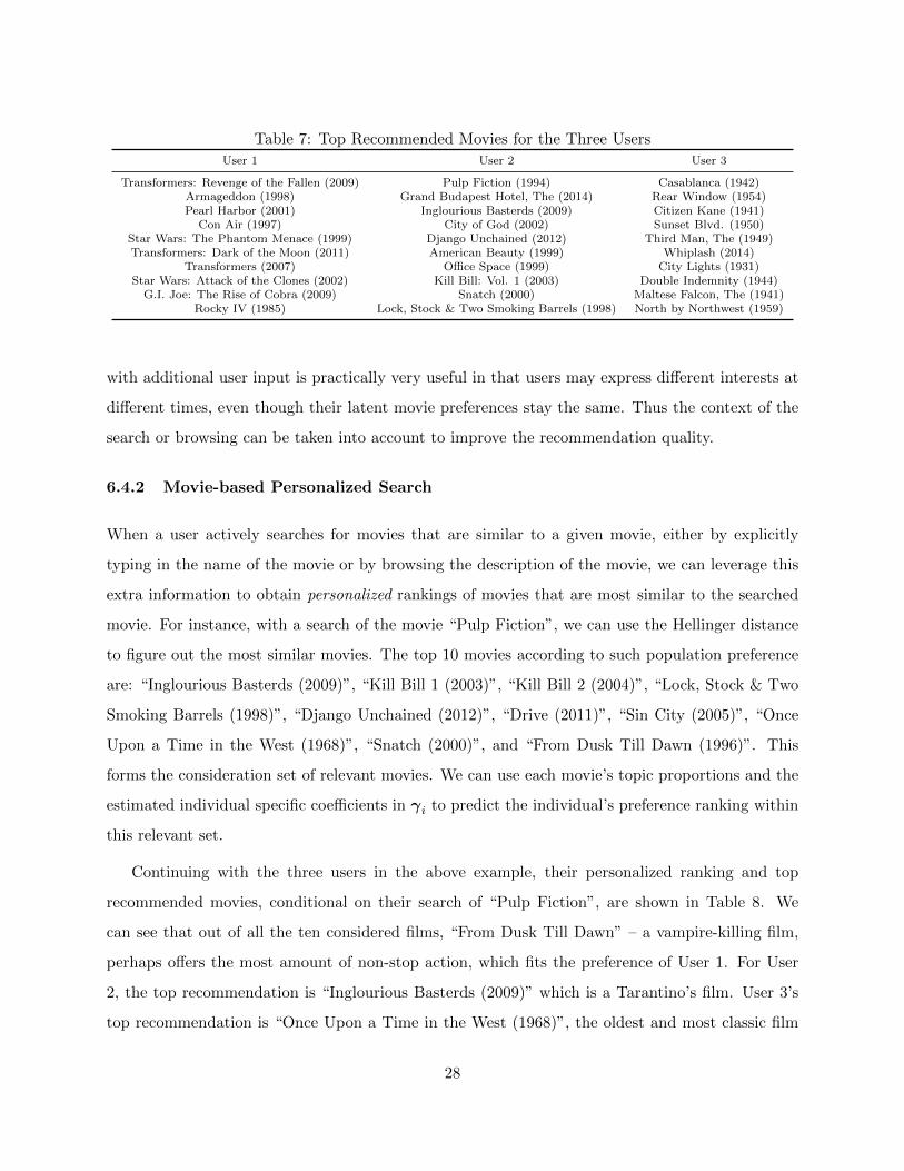
Table 7: Top Recommended Movies for the Three Users
User 1 User 2 User 3
Transformers: Revenge of the Fallen (2009) Pulp Fiction (1994) Casablanca (1942)Armageddon (1998) Grand Budapest Hotel, The (2014) Rear Window (1954)Pearl Harbor (2001) Inglourious Basterds (2009) Citizen Kane (1941)
Con Air (1997) City of God (2002) Sunset Blvd. (1950)Star Wars: The Phantom Menace (1999) Django Unchained (2012) Third Man, The (1949)Transformers: Dark of the Moon (2011) American Beauty (1999) Whiplash (2014)
Transformers (2007) Office Space (1999) City Lights (1931)Star Wars: Attack of the Clones (2002) Kill Bill: Vol. 1 (2003) Double Indemnity (1944)
G.I. Joe: The Rise of Cobra (2009) Snatch (2000) Maltese Falcon, The (1941)Rocky IV (1985) Lock, Stock & Two Smoking Barrels (1998) North by Northwest (1959)
with additional user input is practically very useful in that users may express different interests at
different times, even though their latent movie preferences stay the same. Thus the context of the
search or browsing can be taken into account to improve the recommendation quality.
6.4.2 Movie-based Personalized Search
When a user actively searches for movies that are similar to a given movie, either by explicitly
typing in the name of the movie or by browsing the description of the movie, we can leverage this
extra information to obtain personalized rankings of movies that are most similar to the searched
movie. For instance, with a search of the movie “Pulp Fiction”, we can use the Hellinger distance
to figure out the most similar movies. The top 10 movies according to such population preference
are: “Inglourious Basterds (2009)”, “Kill Bill 1 (2003)”, “Kill Bill 2 (2004)”, “Lock, Stock & Two
Smoking Barrels (1998)”, “Django Unchained (2012)”, “Drive (2011)”, “Sin City (2005)”, “Once
Upon a Time in the West (1968)”, “Snatch (2000)”, and “From Dusk Till Dawn (1996)”. This
forms the consideration set of relevant movies. We can use each movie’s topic proportions and the
estimated individual specific coefficients in γi to predict the individual’s preference ranking within
this relevant set.
Continuing with the three users in the above example, their personalized ranking and top
recommended movies, conditional on their search of “Pulp Fiction”, are shown in Table 8. We
can see that out of all the ten considered films, “From Dusk Till Dawn” – a vampire-killing film,
perhaps offers the most amount of non-stop action, which fits the preference of User 1. For User
2, the top recommendation is “Inglourious Basterds (2009)” which is a Tarantino’s film. User 3’s
top recommendation is “Once Upon a Time in the West (1968)”, the oldest and most classic film
28
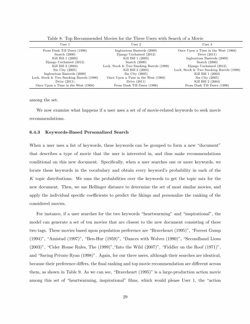
Table 8: Top Recommended Movies for the Three Users with Search of a Movie
User 1 User 2 User 3
From Dusk Till Dawn (1996) Inglourious Basterds (2009) Once Upon a Time in the West (1968)Snatch (2000) Django Unchained (2012) Drive (2011)
Kill Bill 1 (2003) Kill Bill 1 (2003) Inglourious Basterds (2009)Django Unchained (2012) Snatch (2000) Snatch (2000)
Kill Bill 2 (2004) Lock, Stock & Two Smoking Barrels (1998) Django Unchained (2012)Sin City (2005) Kill Bill 2 (2004) Lock, Stock & Two Smoking Barrels (1998)
Inglourious Basterds (2009) Sin City (2005) Kill Bill 1 (2003)Lock, Stock & Two Smoking Barrels (1998) Once Upon a Time in the West (1968) Sin City (2005)
Drive (2011) Drive (2011) Kill Bill 2 (2004)Once Upon a Time in the West (1968) From Dusk Till Dawn (1996) From Dusk Till Dawn (1996)
among the set.
We now examine what happens if a user uses a set of of movie-related keywords to seek movie
recommendations.
6.4.3 Keywords-Based Personalized Search
When a user uses a list of keywords, these keywords can be grouped to form a new “document”
that describes a type of movie that the user is interested in, and thus make recommendations
conditional on this new document. Specifically, when a user searches one or more keywords, we
locate these keywords in the vocabulary and obtain every keyword’s probability in each of the
K topic distributions. We sum the probabilities over the keywords to get the topic mix for the
new document. Then, we use Hellinger distance to determine the set of most similar movies, and
apply the individual specific coefficients to predict the likings and personalize the ranking of the
considered movies.
For instance, if a user searches for the two keywords “heartwarming” and “inspirational”, the
model can generate a set of ten movies that are closest to the new document consisting of these
two tags. These movies based upon population preference are “Braveheart (1995)”, “Forrest Gump
(1994)”, “Amistad (1997)”, “Ben-Hur (1959)”, “Dances with Wolves (1990)”, “Secondhand Lions
(2003)”, “Cider House Rules, The (1999)”,“Into the Wild (2007)”, “Fiddler on the Roof (1971)”,
and “Saving Private Ryan (1998)”. Again, for our three users, although their searches are identical,
because their preference differs, the final ranking and top movie recommendation are different across
them, as shown in Table 9. As we can see, “Braveheart (1995)” is a large-production action movie
among this set of “heartwarming, inspirational” films, which would please User 1, the “action
29

enthusiast”. User 2’s top recommendation is “Into the Wild (2007)”, which features a young
college grad who shuns the material world, cuts off communication with his family, lives off the
land in Alaska, and eventually dies due to food poisoning. Consistent with User 2’s preference,
this film’s production is small, and the storyline and the protagonist actions are unusual. “Saving
Private Ryan (1998)” is the top recommendation for User 3. Its story is based on a historical event
in WWII, which might please our “classics enthusiast”.
Table 9: Top Recommended Movies for the Three Users with Search of Keywords
User 1 User 2 User 3
Braveheart (1995) Into the Wild (2007) Saving Private Ryan (1998)Forrest Gump (1994) Saving Private Ryan (1998) Into the Wild (2007)
Saving Private Ryan (1998) Forrest Gump (1994) Ben-Hur (1959)Dances with Wolves (1990) Braveheart (1995) Braveheart (1995)Secondhand Lions (2003) Cider House Rules, The (1999) Fiddler on the Roof (1971)
Amistad (1997) Amistad (1997) Forrest Gump (1994)Cider House Rules, The (1999) Dances with Wolves (1990) Cider House Rules, The (1999)
Into the Wild (2007) Ben-Hur (1959) Dances with Wolves (1990)Fiddler on the Roof (1971) Secondhand Lions (2003) Amistad (1997)
Ben-Hur (1959) Fiddler on the Roof (1971) Secondhand Lions (2003)
7 Conclusion
In this research, we contribute to the literature on recommendation systems by developing a novel
cross-nested supervised latent Dirichlet allocation topic model that leverages both numerical rating
data and textual data to make movie recommendations. The latent topics are inferred from both
the tag vocabulary and the user ratings, which increase the predictive ability of the topics, and the
use of crowd-sourced tags alleviates the often onerous requirement for the firm-provided product
attributes. We apply this topic model on a datasets of 8.87 million movie ratings, and develop a
new stochastic variational Bayesian approach to estimate the model. We show that the resulting
recommendation model generates much better predictions than the benchmark model, yields a
number of interesting insights regarding user preferences on movies, and requires a short amount
of estimation time, thereby making it useful in actual recommendation contexts.
We also show how our modeling framework can be useful for generating targeted recommenda-
tions for users. In particular, we show how our model can support personalized search for movies
that are similar to a given movie. We show how the topic proportions for a given movie can be
30
used to generate a set of relevant movies that are similar to the focal movie. User level preference
parameters can then be used to generate a unique ordering of the relevant movies for each user,
thus resulting in personalized search rankings.
On the methodology front, we highlight the usefulness of the variational Bayesian framework for
marketing. The rapid growth in data volume, data variety, and crowd-sourcing that characterize
big data has opened new opportunities for deeper learning about customer preferences and for
using predictions obtained from such data for marketing actions. Novel and complex marketing
models such as ours that include many latent variables and parameters are needed to fully capitalize
on the information contained in the big data settings. Scalable inference therefore becomes one
of the major challenges that stems from the big data and big learning environments, and the
traditional approaches in Bayesian inference, such as MCMC, suffer from computational bottleneck
for practical big data applications. In contrast, by integrating the state-of-the-art advances of
variational Bayesian inference, we show how stochastic VB can offer a versatile solution to the
scalability and computational challenge in estimating complex marketing models for big data,
particularly so in the context of product recommendation on the internet.
While we focus on stochastic VB in the current paper, other methods to tackle scalability issues
are being actively investigated in the Bayesian literature. VB methods, especially those that are
based on fully factorized mean-field approximations can result in an underestimation of parameter
uncertainty. However, they are useful in marketing situations where predictive performance in a
managerially realistic amount of time is of critical importance. Many such scenarios are documented
in Cui and Curry (2005). Other recently proposed methods for scalable inference include stochastic
gradient based MCMC that relies on subsampling or divide-and-conquer approaches to speed up
MCMC algorithms. While these are active research areas, their utility in complex hierarchical
settings such as ours is yet to be demonstrated. In the end, all these scalable big data solutions entail
an important trade-off between unlimited accuracy in unlimited time and a good approximation
within a reasonable time, and different decision contexts imply different resolutions of this trade-
off (Bottou and Bousquet 2007). We leave a thorough comparison of these approaches for future
research.
31

References
Ansari, A., S. Essegaier and R. Kohli (2000). “Internet recommendation systems,” Journal ofMarketing Research, 37(3), 363-375.
Ansari, A., Y. Li and J. Z. Zhang (2016). “Stochastic Variational Bayesian Inference for Big DataMarketing Models,” Working Paper.
Bishop, C. (2006). Pattern Recognition and Machine Learning, New York, Springer.
Blei, D. and J. McAuliffe (2007). “Supervised topic models,” Neural Information ProcessingSystems, 21.
Blei, D., A. Ng and M. Jordan (2003). “Latent Dirichlet allocation,” Journal of Machine LearningResearch, 3, 993-1022.
Bodapati, A. V. (2008). “Recommendation systems with purchase data,” Journal of MarketingResearch, 45(1), 77-93.
Bottou, L. and O. Bousquet (2007). “The tradeoffs of large-scale learning,” Advances in neuralinformation processing systems, 20.
Braun, M. and J. McAuliffe (2010). “Variational inference for large-scale models of discretechoice,” Journal of the American Statistical Association, 105(489), 324-335.
Chung, J. and V. R. Rao (2012). “A general consumer preference model for experience products:application to internet recommendation services,” Journal of Marketing Research, 49(3), 289-305.
Chung, T. S., R. T. Rust and M. Wedel (2009). “My mobile music: an adaptive personalizationsystem for digital audio players,” Marketing Science, 28(1), 52-68.
Cui, D. and D. Curry (2005). “Prediction in marketing using the support vector machine,”Marketing Science, 24(4), 595-615.
Desrosiers, C. and G. Karypis (2011). “A comprehensive survey of neighborhood-based recom-mendation methods,” Recommender Systems Handbook, 107-144.
Dzyabura, D. and J. R. Hauser (2011), “Active machine learning for consideration heuristics,”Marketing Science, 30(5), 801-819.
Gaivoronski, A. (1988). “Implementation of stochastic quasigradient methods,” Numerical Tech-niques for Stochastic Optimization, 313-352, New York, Springer-Verlag.
Harper, M. and J. A. Konstan (2015). “The MovieLens datasets: history and context,” ACMTransactions on Interactive Intelligent Systems, 5(4).
Hastings, W. K. (1970). “Monte Carlo sampling methods using Markov chains and their applica-tions,” Biometrika, 57(1), 97-109.
32
Hoffman, M., D. M. Blei, C. Wang and J. Paisley (2013). “Stochastic variational inference,”Journal of Machine Learning Research, 14(1), 1303-1347.
Jordan, M. I., Z. Ghahramani, T. S. Jaakkola, L. K. Saul (1999). “An introduction to variationalmethods for graphical models,” Machine Learning, 37, 183-233.
Koren, Y. and R. Bell (2011). “Advances in collaborative filtering,” Recommender Systems Hand-book, 145-186.
Kullback, S. and R. A. Leibler (1951). “On information and sufficiency,” The Annals of Mathe-matical Statistics, 22, 79-86.
Lee, T. Y. and E. T. Bradlow (2011). “Automated marketing research using online customerreviews”, Journal of Marketing Research, 48(5), 881-894.
Lops, P., M. Gemmis and G. Semeraro (2011). “Content-based recommender systems: state ofthe art and trends,” Recommender Systems Handbook, 73-105.
Minka, T. P. (2001). “A family of algorithms for approximate Bayesian inference,” Ph.D. Thesis,MIT.
Murphy K. P. (2012). Machine Learning: A Probabilistic Perspective, The MIT Press.
Ormerod, J. T. and M. P. Wand (2010). “Explaining variational approximations,” The AmericanStatistician, 64(2), 140-153.
Rezende, D. J., S. Mohamed and D. Wierstra (2014). “Stochastic backpropagation and approxi-mate inference in deep generative models,” Proceedings of the 31st International Conferenceon Machine Learning, 32.
Robbins, H. and S. Monro (1951). “A stochastic approximation method,” Annals of MathematicalStatistics, 22, 400-407.
Rossi, P. E., R. E. McCulloch and G. M. Allenby (1996). “The value of purchase history data intarget marketing,” Marketing Science, 15(4), 321-340.
Spall, J. (2003). Introduction to Stochastic Search And Optimization: Estimation, Simulation,and Control, John Wiley and Sons.
Tan, L. S. L. (2015). “Stochastic variational inference for large-scale discrete choice models usingadaptive batch sizes,” Statistics and Computing, 1-21.
Tirunillai, S. and G. J. Tellis (2014). “Mining marketing meaning from online chatter: strategicbrand analysis of big data using latent Dirichlet allocation”, Journal of Marketing Research,51(4), 463-479.
Toulis, P. and E. M. Airoldi (2016). “Implicit stochastic gradient descent,” Annals of Statistics,forthcoming.
Ying, Y., F. Feinberg and M. Wedel (2006). “Leveraging missing ratings to improve online rec-ommendation systems,” Journal of Marketing Research, 43(3), 355-365.
33

Zhang, J. and L. Krishnamurthi (2004). “Customizing promotions in online stores,” MarketingScience, 23(4), 561-578.
34
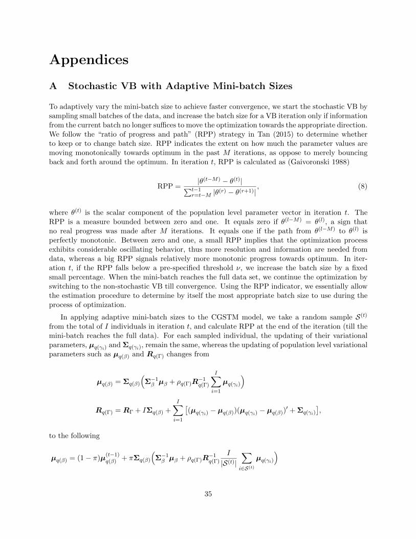
Appendices
A Stochastic VB with Adaptive Mini-batch Sizes
To adaptively vary the mini-batch size to achieve faster convergence, we start the stochastic VB bysampling small batches of the data, and increase the batch size for a VB iteration only if informationfrom the current batch no longer suffices to move the optimization towards the appropriate direction.We follow the “ratio of progress and path” (RPP) strategy in Tan (2015) to determine whetherto keep or to change batch size. RPP indicates the extent on how much the parameter values aremoving monotonically towards optimum in the past M iterations, as oppose to merely bouncingback and forth around the optimum. In iteration t, RPP is calculated as (Gaivoronski 1988)
RPP =|θ(t−M) − θ(t)|∑t−1
r=t−M |θ(r) − θ(r+1)|, (8)
where θ(t) is the scalar component of the population level parameter vector in iteration t. TheRPP is a measure bounded between zero and one. It equals zero if θ(l−M) = θ(l), a sign thatno real progress was made after M iterations. It equals one if the path from θ(l−M) to θ(l) isperfectly monotonic. Between zero and one, a small RPP implies that the optimization processexhibits considerable oscillating behavior, thus more resolution and information are needed fromdata, whereas a big RPP signals relatively more monotonic progress towards optimum. In iter-ation t, if the RPP falls below a pre-specified threshold ν, we increase the batch size by a fixedsmall percentage. When the mini-batch reaches the full data set, we continue the optimization byswitching to the non-stochastic VB till convergence. Using the RPP indicator, we essentially allowthe estimation procedure to determine by itself the most appropriate batch size to use during theprocess of optimization.
In applying adaptive mini-batch sizes to the CGSTM model, we take a random sample S(t)
from the total of I individuals in iteration t, and calculate RPP at the end of the iteration (till themini-batch reaches the full data). For each sampled individual, the updating of their variationalparameters, µq(γi) and Σq(γi), remain the same, whereas the updating of population level variationalparameters such as µq(β) and Rq(Γ) changes from
µq(β) = Σq(β)
(Σ−1β µβ + ρq(Γ)R
−1q(Γ)
I∑i=1
µq(γi)
)
Rq(Γ) = RΓ + IΣq(β) +
I∑i=1
[(µq(γi) − µq(β))(µq(γi) − µq(β))
′ + Σq(γi)
],
to the following
µq(β) = (1− π)µ(t−1)q(β) + πΣq(β)
(Σ−1β µβ + ρq(Γ)R
−1q(Γ)
I
|S(t)|∑i∈S(t)
µq(γi)
)
35

Rq(Γ) = (1− π)R(t−1)q(Γ) + π
{RΓ + IΣq(β) +
I
|S(t)|∑i∈S(t)
[(µq(γi) − µq(β))(µq(γi) − µq(β))
′ + Σq(γi)
]}.
In above, the exponential average between the current and the last iterations with weight π ensuresthe convergence of the stochastic optimization (Hoffman et al. 2013). The multiplier I/|S(t)| rescalesthe intermediate estimate as if the entire data (i.e., all individuals) are used for the current updating.The non-stochastic version of VB is recovered when π = 1 and |S(t)| = I, i.e., the mini-batchincludes all individuals from the original dataset. In order to move the parameter estimates quicklytowards the optimum, we further allow the RPP threshold ν and the weight π to linearly vary withthe mini-batch size across iterations, reflecting the higher tolerance and less precision we are willingto accept in early VB iterations.
B Stochastic VB Updates for the CGSTM Model
We estimate the CGSTM model via stochastic VB with adaptive mini-batch sizes. In each iteration,we sample a subset of users S(t) using the RPP strategy discussed in Appendix A. Denote thedocuments rated by the sampled individuals of current iteration as Ds, where Ds = ∪i∈S(t)Di. Wefirst update the variational parameters associated with document d, ∀d ∈ Ds. Let ud = logαd, thusud ∼ N (x′dν, δ
2). In particularly, the ADSVB method detailed in Ansari, Li and Zhang (2016) isapplied to update the variational parameters in q(ud) = N (µq(ud), σ
2q(ud)). We derive the gradient
for ADSVB as
∂ log p(ωd, ud)
∂ud= Keud
(Ψ(Keud)−Ψ(eud)
)+eud
K∑k=1
(Ψ(ζdk)−Ψ(
K∑k=1
ζdk))−aq(δ2)
aq(δ2)
(ud−x′dµq(ν)
),
(9)where Ψ(·) is the digamma function.
Within document d, the variational parameters for topic proportions ωd, ∀d ∈ Ds are updatedby,
ζd = exp{µq(ud) + 0.5 σ2q(ud)}+
Nd∑n=1
φdn. (10)
The variational parameters for topic assignment of word wdn are calculated by
φdn ∝ τn exp{
Ψ(ζd) +1
Nd
aq(σ2)
bq(σ2)
∑i∈Id
ydiµq(γi)
− 1
2N2d
aq(σ2)
bq(σ2)
∑i∈Id
[2(Σq(γi) + µq(γi)µ
′q(γi)
)φd,−n + µ2q(γi)
+ diag(Σq(γi))]}, (11)
where, φd,−n =∑
j 6=nφj , and Id denotes the sampled individuals who rated document d. Then,
36

we update the variational parameters of the individual coefficient γi for every sampled user,
Σ−1q(γi)
= ρq(Γ)R−1q(Γ) +
aq(σ2)
bq(σ2)E(A′iAi) (12)
µq(γi) = Σq(γi)
[ρq(Γ)Rq(Γ)µq(β) +
aq(σ2)
bq(σ2)E(Ai)yi
], (13)
where E(Ai) is a |Di|×K matrix with vectors φd on each row, and E(A′iAi) =∑
d∈Di
1N2
d
[∑m 6=nφdnφ
′dm+
diag(φdn)].
Next, we update the population level parameters using the weighted average discussed in SectionA. Specifically, the topic distribution is given by,
τkw ∝ (1− π)τ(t−1)kw + π
D∑d=1
Nd∑n=1
1(wdn = w)φdnk. (14)
The variational parameters for the population covariance matrix Γ are updated by,
ρq(Γ) = ρΓ + I (15)
Rq(Γ) = (1− π)R(t−1)q(Γ) + π
{RΓ + IΣq(β) +
I
|S(t)|∑i∈S(t)
[(µq(β) − µq(γi))(µq(β) − µq(γi))
′ + Σq(γi)
]}(16)
The variational parameters for the population mean β are given by,
Σ−1q(β) = Σ−1
β + I · ρq(Γ)R−1q(Γ) (17)
µq(β) = (1− π)µ(t−1)q(β) + πΣq(β)
[Σ−1β µβ + ρq(Γ)R
−1q(Γ)
I
|S(t)|∑i∈S(t)
µq(γi)]. (18)
The variational parameters for the error variance σ2 are calculated as,
aq(σ2) = aσ2 +1
2
D∑d=1
Id (19)
bq(σ2) = (1− π)b(t−1)q(σ2)
+ π{bσ2 +
1
2
I
|S(t)|∑i∈S(t)
(‖yi − E(Ai)µq(γi)‖
2 + Tr[E(A′iAi)Σq(γi)
])}, (20)
where Id denotes the total number of individuals who rated document d.
The variational parameters for the aggregate attribute coefficient ν are given by,
Σ−1q(ν) = Σ−1
ν +aq(δ2)
bq(δ2)X ′X (21)
37

µq(ν) = (1− π)µ(t−1)q(ν) + πΣq(ν)
[Σ−1ν µν +
I
|S(t)|aq(δ2)
bq(δ2)X ′Ds{µq(ud)}d∈Ds ]. (22)
Lastly, the variational parameters for the error variance δ2 are calculated as,
aq(δ2) = aδ2 +D
2(23)
bq(δ2) = (1− π)b(t−1)q(δ2)
+ π[bδ2 +
1
2
I
|S(t)|∑d∈Ds
((µq(ud) − x′dµq(ν))
2 + x′dΣq(ν)xd + σ2q(ud)
)]. (24)
38