Comments Welcome

Probabilities, Probits and the Timing of Currency Crises

Susan M. Collins

GeorgetownUniversity The Brookings Institution and NBER*

Draft: March 2003

Abstract A growing empirical literature studies determinants of the probability of a currency crisis, often searching for a combination of indicators to provide an early warning system (EWS). The existing work frequently relies on discrete choice specifications, such as probits, that do not incorporate the time dimension of the occurrence of currency crises and that are not derived from an underlying behavioral model. These ad hoc specifications are defined over a fixed horizon (such as 24 months) and provide no consistent way of estimating crisis probabilities over other horizons (such as 3, 12 or 36 months). This paper shows how a probit can be interpreted in terms of restrictions on a simple threshold model of the timing of a currency crisis, that is based on recent theoretical models of crises. Using data for 25 emerging markets, the threshold specification is shown to fit better than either a probit specification, or the exponential waiting time distribution implied by a poisson model of crises. In addition, the threshold model can be used to generate estimates of the probability of a crisis occurring over any future time horizon, as a function of current indicators. _________________________ * Much of the work for this paper was done while I was visiting the IMF. I would like to thank Andrew Berg, Robert Flood, Olivier Jeanne, Kenneth Kletzer, Sam Oularis and Catherine Patillo for helpful discussions and suggestions. I am also grateful to Andrew Berg and Catherine Pattillo for providing their data, and to Haiyan Shi for research assistance. Views expressed do not necessarily represent those of any of the institutions listed.

- 1 -

1. Introduction

In the aftermath of several severe currency crises affecting countries around the globe, there

has been an explosion of empirical studies of crises. This work has focused on a variety of interesting

and important issues, including the following. How should crises be defined? Are crises predictable?

What explanatory variables should be included in the empirical analysis? Can an early warning

system (EWS) be designed that would signal the increased likelihood of a crisis? But although some

papers also address the appropriate econometric specification for modeling the probability of a crisis,

the most frequent estimation approach has been some form of probit (or logit). The simplest versions

define the dependent variable as one or zero depending on whether the event (a currency crisis) does

or does not occur within a particular time period. In other words, many studies use a specification

designed to study the probability of a �discrete choice� so as to study the probable occurrence of a

discrete event within a given time period. While this approach may provide useful descriptive

information, it has a number of shortcomings. In particular, it is not clear how to interpret a discrete

choice framework in the context of an event that unfolds over time. This framework is not based on a

behavioral model of what causes a crisis. It does not provide a consistent means of studying the

probability of a crisis at different time horizons � the timing of the crisis. And estimation typically

ignores information about when crises actually occurred.

This paper has three main tasks. First, building on Collins (1992) it uses a threshold model of

currency crises to develop an econometrically tractable model of the timing of a crisis. This threshold

model is consistent with many first generation models of currency crises as well as some

specifications of second generation models. The paper then shows that a probit specification can be

interpreted in terms of restrictions on the crisis probability implied by the threshold model. Second, a

simple version of the threshold model is tested against a probit specification, using data for 25

emerging market economies during the period 1985-98. The threshold model is also tested against

another alternative -- a poisson model of crises. Finally the paper estimates the full version of the

threshold model and discusses the results. In particular, the estimates are used to construct the

- 2 -

implied evolution of the probability of a crisis over different time horizons, and implications for

selected countries are discussed.

It is important to note at the outset a number of things that this paper does not attempt to do.

It breaks no new ground in terms of how currency crises should be defined, nor does it introduce

additional explanatory variables. Instead, data from previous, well known work by Berg and Pattillo

(1999a,b) are used for the estimations so that the threshold specification can be tested against an

existing probit analysis. Also, and unlike much of the EWS literature, this work is not intended to

provide an alternative approach to forecasting currency crises. Indeed, non-parametric and other

methods may well out-perform more structural model based equations. No effort is made to examine

the forecasting ability of the threshold model, either in or out of sample.

The empirical literature on currency crises is large and growing rapidly.1 It can be divided

loosely into four groups, discussed briefly below. (Some of the studies listed employ more than one

methodology). One set of studies uses the signals -- or indicators -- approach, developed by

Kaminsky, Lizondo and Reinhart (1998). The approach has been extended by Kaminsky and

Reinhart (1999), Kaminsky (1999) and Edison (2000) among others. Borensztein et. al. (2000)

describes the IMF usage of this approach as one of its EWS models. These studies define a crisis

indicator equal to one if a crisis occurs and zero otherwise. They next construct zero/one indicator

variables for a set of explanatory variables. The indicators can then be used to forecast crises.

The second, and most numerous, set of studies uses limited dependent variable techniques

(probit or logit) to relate the probability of a crisis to a set of explanatory variables. Early studies of

exchange regime collapse using probit include Eichengreen, Rose and Wyplosz (1996), who study 20

industrial countries, and Frankel and Rose (1996) who study 105 developing countries. Klein and

Marion (1997) use a logit specification to study exchange rate changes in Latin America. After the

crises in Asia exploded, Berg and Patillo (1999a, 1999b) undertook a series of studies that compared

probit analysis with the signals approach. Advantages are that the explanatory variables need not be

dichotomous, that the approach incorporates correlations among variables, and that standard statistical

1 Kaminsky, Lizondo and Reinhart (1998) provide a survey of empirical studies written prior to 1997, while Abiad (2003) surveys much of the more recent empirical literature.

- 3 -

methods can be used to examine goodness of fit and to test hypotheses. (A variety of difficulties with

this approach will be discussed below.)

Berg and Patillo�s conclusion -- that a probit is generally preferred to the signals approach --

seems to have generated a large volume of empirical work using discrete choice specifications.

Recent analyses that use probits to estimate the probability of currency crises include: Block (2002),

Caramazza, Ricci and Salgado (2000), Esquival and Larraín (1998), Kamin, Schindler and Samuel

(1999), Manuel and Rocha (2000), Milesi-Ferretti and Razin (2000), Mulder, Perrelli and Rocha

(2002), as well as Borensztein et. al. (2000). Leblang (2001?) uses a special form of probit,

appropriate for samples in which events (crises) are rare. Studies using logit specifications include

Goldfajn and Valdez (1997), Kumar, Moorthy and Perraudin (2002) and Weller (2001). Some

authors use discrete choice specifications with more that two possible outcomes (for instance,

tranquil, crisis and post crisis states). For instance, Kaufman, Mehrez and Schmukler (2000) use an

ordered probit specification while Bussiere and Fratzscher (2002) as well as Eliasson and Krauter

(2001) use multinomial logits. While these studies all used pooled or panel data, others such as Sachs,

Tornell and Velasco (1996) use probits on a cross section to study determinants of crisis severity.

These studies incorporate a wide range of explanatory variables, suggested by first and second

generation models of crisis, as well alternative frameworks such as political economy approaches.

A third, considerably smaller set of empirical studies builds on an underlying behavioural

model of currency crises. Most of these are case studies of individual countries. The following

authors estimate a full structural model, based on first generation models of currency crises: Blanco

and Garber (1986), Cumby and van Wijnbergen (1989), Goldberg (1994) and Otker and

Pazabariouglu (1997). Flood and Marion (1994) develop and estimate a model of the timing and size

of devaluation for a set of Latin American countries. Some more recent work is based on second

generation models of currency crises. Of particular note here is Eichengreen and Jeanne (2000) who

develop and estimate an escape-clause model of the 1931 sterling crisis. Authors who have used

switching models to capture the possibility of multiple equilibria include Jeanne and Masson (1998)

as well as Abiad (2003), Fratzscher (1999) and Martinez-Peria (2002).

Finally, a recent paper by Tudela (2001) applies duration methods (a proportional hazard

specification) to study determinants of the length of spells between exchange rate crises. Widely

used in other areas such as the study of unemployment, this approach is very flexible, facilitates

- 4 -

analysis of possible time-dependence of the duration of spells and provides a means to estimate the

probability of a crisis at different time horizons (in other words, the timing of a crisis). However,

like the discrete choice approaches, it is ad hoc and not based on an underlying model.

The remainder of this paper is composed of six sections. Section 2 discusses theoretical

currency crisis models. It then develops the threshold model, that is amenable to empirical analysis.

Section 3 shows how a probit specification can be interpreted in terms of the probability of a crisis

derived from the threshold model. Section 4 discusses data and some of the estimation issues.

Section 5 tests the simple version of threshold model against two alternatives. Section 6 presents and

discusses estimation of the full threshold model. Section 7 concludes.

2. Modeling Currency Crises

2.1 Two simple approaches

This section develops two alternatives approaches to specifying the probability of a crisis.

One is the popular, though not model based, probit specification. The second uses the convenient

poisson formulation.

Probit

Following many previous studies, crisis probabilities can be specified using a probit structure.

There is assumed to be some underlying, unobservable process: y* for each country i. In the current

application, its position at time t+k depends on information available at time t, as well as a random

error term, which is i.i.d:

( )2,,,, ,0~,* σβ NuuXy ktiktitikti +++ += (1)

Assume that if yi,t +k> 0, then a crisis is observed, and define C24 = 1 if a crisis occurs within 24

months, and 0 otherwise. Thus, k has been set equal to 24 months (which will later be defined as

�one period�) Then the probability that no crisis occurs within 24 months of t is:

( ) ( )σβ /)024Pr( ,Pr

tiXFC −Φ=⋅== (2)

- 5 -

The probit framework is easily estimated. However, it only specifies the probability of a crisis over a

specific time horizon (in this case, 24 months), providing no consistent means of uncovering the

probabilities of a crisis over different horizons. In other words, the length of the horizon of interest is

not incorporated into the specification for the probability of an event (crisis). The probit is also not

based on any underlying theoretical model of crises.

Poisson Model

Assuming that crises can be described as events in a poisson process provides a second very

simple specification for relating the probability of a crisis to observable country characteristics.2

Define the mean rate of arrival of events as ηi,t for country i in month t, where ηi,t = Xi,t β depends on

conditions in country i at time t. (Subscripts will be omitted below where it is not confusing to do

so.) Starting at any time t, the behavior of the process during t+k is independent of behavior up to

time t. Let t+T be the time of the first event after t. Then for any k, the probability that no event has

occurred by t+k, given η, can be shown to have an exponential distribution, FE :

( ) ( ) ( )kkFkT E ηη −==> exp;Pr (3)

The cumulative probability distribution for the time of a crisis, is thus {1- exp(-ηk)} and the

associated probability density is {η exp(-ηk)}. Clearly the probability of a crisis within k=24 months

does depend on k.

Two appealing features of the poisson formulation are that it provides a probability

distribution for the timing of crises (T) and that it is easily estimated. However, the single parameter

exponential distribution is not very flexible. The probability of a poisson event is most likely to occur

in the near future, and declines monotonically thereafter. This specification is not appropriate for

modeling an event for which the probability is initially small, then rises for a time before declining.

2 Cox and Miller (1995, chapter 4) is one source for a detailed discussion of the poisson model.

- 6 -

2.2 Models of Currency Crises

This section provides a brief overview of some theoretical models of currency crises. The

intent is not to be comprehensive. The relevant body of work is very extensive and is growing

rapidly.3 Nor is the intent to reproduce formal derivations of existing models � readers are referred to

particular papers for details. Instead, I present an overview of some key parts of the literature, as a

motivation for the approach that taken here. Following what has become standard terminology, I

begin with �first-generation� models of the timing of currency crises, and then turn to the �second

generation�. In this discussion, I will assume that once the fixed (or managed) rate is abandoned, the

exchange rate is allowed to float freely.

First generation models

This set of models of currency crises focuses on how long a country can continue to defend a

fixed exchange rate in the context of expansionary macroeconomic (monetary and fiscal) policy that

gradually depletes the reserve stock and is inconsistent with indefinite maintenance of a fixed

exchange rate. A key insight of this literature is that speculators will �attack� the central bank�s

remaining stock of foreign exchange reserves as soon as it becomes profitable for them to do so - and

this will typically occur before the reserve depletion would have exhausted them. Further, such

attacks may be rational and fully anticipated.4

A common feature of these models is that the time of a speculative attack is determined by

the first time at which the underlying shadow exchange rate becomes at least as depreciated as the

current fixed exchange rate. This shadow exchange rate is simply the exchange rate that would

prevail each period if reserves had been exhausted, and the exchange rate were to float. In early

versions, the equation for the shadow exchange rate was derived from a simple monetary model of a

small open economy. But numerous extensions have incorporated other features, such as a real side,

3 Agenor, Bhandari and Flood (1992), Flood and Marion (1999) and Jeanne (2000) provide useful summaries and discussions of the theoretical literature on balance of payments crises.

4 This literature was launched by Krugman (1979) who adapted a paper by Salant and Henderson (1978) to the foreign exchange market. The approach was formalized by Flood and Garber (1984). The large literature that arose has been summarized by Agenor, Bhandari and Flood (1992), Blackburn and Sola (1993), and more recently by Folld and Marion (1999) and Jeanne (2000).

- 7 -

deviations from PPP, a government budget constraint, capital controls and/or an additional country.

Many versions of the model are linear, expressing the (log of) the shadow exchange rate as a simple

linear function of fundamentals, which grow at a constant rate over time. Stochastic extensions of the

model typically incorporate a normally distributed error term, with mean zero and constant variance.

Some first generation models also incorporate contingent government policies, giving rise to the

possibility of multiple equilibria.

These models point to a number of variables that would provide good indicators of the

relevant fundamentals for empirical analysis. In particular, excess domestic credit expansion will

lead to cumulated domestic inflation, and an increasingly overvalued real exchange rate. Countries

more likely to experience a crisis will tend to have a lower level of official reserves and, particularly

in versions with capital controls, larger current account deficits.

Assume that the (log) shadow exchange rate, st , can be expressed as follows:

st = f t + α ts t/dt (4)

where the shadow exchange rate, is expressed as the domestic price of foreign exchange, ts t/dt is the

expected exchange rate change, given information available time t, and f t is a stochastic

fundamental. (This formulation can easily be derived from a standard monetary model.)

Furthermore, assume that f t can be characterized as Brownian motion with drift:

d ft = δ dt + σ d zt (5)

ft = ft0 + δ (t- t0) + σ ( zt-t0 - zt0) (6)

where zt is a standard Weiner process, and δ and σ are both constants. Define k = (t- t0), k ≥ 0 is

the amount of time that has elapsed since the process was initially observed at t0. Then the solution

for the path of st can be shown to be:

st = st0+k = α δ + ft0 + δ k + σ ( zt-t0 - zt0) (7)

And at any point in time t = t0 + k ≥ t0 , the gap between the current fixed exchange rate, S, and the

shadow exchange rate is:

- 8 -

S - st0+k = Dt0 - δ k - σ ( zt-t0 - zt0) (8)

where Dt0 = ( S - α δ - ft0 )

The first term on the right hand side of (8) is simply the initial distance (at t0 ) of the shadow

exchange rate from S. This depends on the position of the fundamental at time t0 as well as on its rate

of drift, δ. Clearly, this distance will change with t0, even if δ.=0. In the empirical analysis, this

distance will be assumed to be a linear function of observable country characteristics. The second

term, δ k , depends on the drift as well as on the amount of time elapsed , k. In the empirical

analysis, three possibilities for the drift are considered: setting the drift equal to zero, constraining the

drift to equal a constant (both for different t0 and across countries as well as for different k, given t0)

Finally, we will allow drift to be a (linear0 function of country i�s characteristics at time t0 � while

still constraining it to be constant for different values of k.. The final term in (8) captures the

influence of stochastic shocks. In section 2.3,

Second generation models

However, a number of real world crises do not seem to �fit� the first generation models.

Indeed, there continue to be debates over the extent to which crises in the EMS in the early 1990s and

in some Asian countries in the late 1990s can be attributed to deteriorating fundamentals. The issue

may be less the government�s ability to continue defending the fixed exchange rate than its

willingness to do so. Second generation 5 models highlight the implications of a conflict in

government�s policy objectives rather than an inherent conflict in its chosen policy instruments. The

government is typically treated as an optimizing agent with multiple domestic objectives. Such a

government may choose to abandon a fixed exchange rate, rather than being forced to do so because

of deteriorating fundamentals.6

Some of these models identify three ranges of underlying fundamentals. In the extreme

ranges, the probability of a crisis is zero (one), because a speculative attack would not (would always)

5 More recently, third generation models highlight the role of balance sheet effects.

6 In particular, see Obstfeld (1994, 1997), Krugman (1997), Drazen (1999), Masson (1998), and Eichengreen and Jeanne (2000). Flood and Marion (1998) and Jeanne (2000) provide summaries.

- 9 -

cause the exchange rate to collapse. In an intermediate range, a crisis is possible. But whether, and if

so when, a crisis actually occurs depends on issues such as investor �confidence�, information

dissemination, and extent of coordination among speculators. There need be no positive trend in

fundamentals for a crisis to occur.

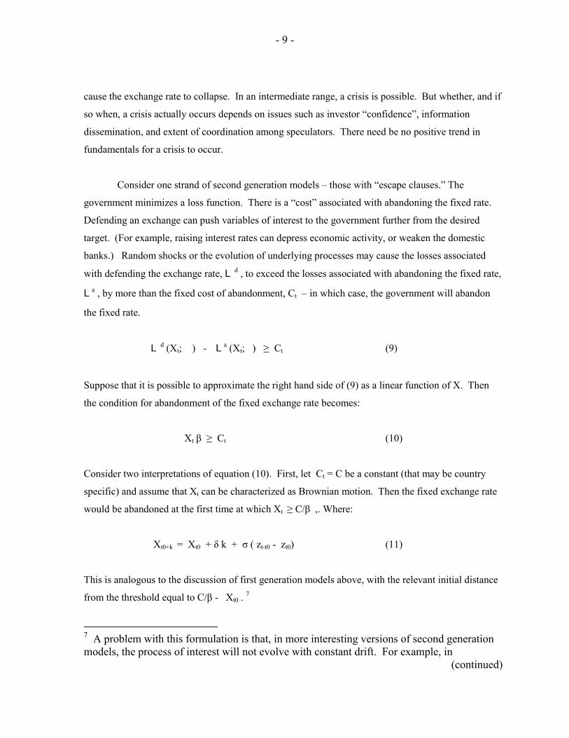
Consider one strand of second generation models � those with �escape clauses.� The

government minimizes a loss function. There is a �cost� associated with abandoning the fixed rate.

Defending an exchange can push variables of interest to the government further from the desired

target. (For example, raising interest rates can depress economic activity, or weaken the domestic

banks.) Random shocks or the evolution of underlying processes may cause the losses associated

with defending the exchange rate, L d , to exceed the losses associated with abandoning the fixed rate,

La , by more than the fixed cost of abandonment, Ct � in which case, the government will abandon

the fixed rate.

L d (Xt; ) - La (Xt; ) ≥ Ct (9)

Suppose that it is possible to approximate the right hand side of (9) as a linear function of X. Then

the condition for abandonment of the fixed exchange rate becomes:

Xt β ≥ Ct (10)

Consider two interpretations of equation (10). First, let Ct = C be a constant (that may be country

specific) and assume that Xt can be characterized as Brownian motion. Then the fixed exchange rate

would be abandoned at the first time at which Xt ≥ C/β ,. Where:

Xt0+k = Xt0 + δ k + σ ( zt-t0 - zt0) (11)

This is analogous to the discussion of first generation models above, with the relevant initial distance

from the threshold equal to C/β - Xt0 . 7

7 A problem with this formulation is that, in more interesting versions of second generation models, the process of interest will not evolve with constant drift. For example, in

(continued)

- 10 -

A second interpretation treats the abandonment cost as a stochastic process, with drift = 0.

Ct0+k = C + σ ( zt-t0 - zt0) (12)

Given the current state of the economy, the fixed rate will be abandoned if the cost drops far enough.

Thus becomes more likely the smaller the current distance from the threshold, C/β - Xt0 . This is

also analogous to the discussion above.

Thus, at least a stylized version of a second generation (escape clause) model of a currency

crisis can also be thought of in terms of a first passage time. The time of a crisis will be determined

by the first time at which a variable crosses a threshold. However, trend movement in this variable

need not be an important part of the story. But a change in economic conditions and/or investor

confidence can move the economy closer to the threshold, thereby raising the probability of a shock

large enough to trigger a crisis.

This formulation points to a somewhat different set of variables that would influence the

probability of a crisis. These are factors related to the government�s perceived cost of defending the

exchange rate, which could include unemployment, banking sector fragility and/or the magnitude of

short-term public debt. However, other economic indicators such as the level or rate of change of

reserves, could also be expected to influence investor confidence. This makes it exceedingly difficult

to identify indicators which would be relevant under a second generation framework, but not under a

first generation one, suggesting that it may be difficult to distinguish between the two in the context

of the threshold timing framework, developed in the next section.

Eichengreen and Jeanne (2000), the probability that the fixed exchange rate is abandoned by the central bank in period t is equal to the probability that next period�s unemployment rate exceeds a bound if the exchange rate is defended. However, the process for unemployment depends in part on the endogenous formation of expectations that the fixed exchange rate will be abandoned, wqhich will change with distance from the threshold.

- 11 -

2.3 Threshold model of the timing of crises

Each country is assumed to have a crisis when an unobservable process crosses a threshold.

This process, or latent variable, would have somewhat different interpretations under first than under

second generation models of currency crises. (I return to this issue below, in the discussion of how to

implement the threshold model.) However, to simplify the discussion, I focus here on the first

generation formulation in which the underlying variable is the shadow exchange rate. Its behavior

over (t0+k), k ≥ 0, given information about the process available at time t0 is given by equation (7).

The discussion here focuses on a single country, omitting the subscript i.

In the absence of a crisis, the process st0 +k will also be normally distributed, as shown in

equation (1).

A crisis is assumed to occur the first time at which the latent variable st0 +k hits a critical level, S.

Thus, S can be thought of as an absorbing barrier for the Brownian motion process. Define Tt0 is the

time until a crisis (the first passage time), such that st0+T = S.

Two possible scenarios are depicted in Figure 1. Case A shows an economy in which st0 +k is

approaching the threshold at a mean rate δA > 0. The expected time of crisis is E(ΤA) = (S - st0 +T) /δA

= Dt0 /δA. This would occur in the absence of any random shocks. In scenario A, the actual crisis

occurs at Τ < E(ΤA). In case B, st0 +k is drifting away from the critical level S at mean rate δB < 0 and

no crisis occurs. It would take a large shock to cause the process to rise to S, triggering a crisis.

(There is a non-zero probability in case B that zt(k) never reaches S and there will never be a crisis.)

Given the absorbing barrier, st0 +k will not be normally distributed. Instead, its probability

density function can be shown to have an additional term, as given by equation (14).8

8 See Cox and Miller (1995, chapter 5), Chhikara and Folks (1989, chapter 3) for derivations and further discussion of the behavior of a Brownian motion process with an absorbing barrier and of the related first passage time distribution.

) k ,k +sN( s 2tttkt σδ 000 ~+ (13)

- 12 -

( )

−

k2k-D2z-(x - D 2 +

k2k-z-(x-

k2 1

= ,D,z ; x=(k)zp

t

ttt

t

tt

t

tt

t

ttttt

222

2

exp)exp

,

σδ

σδ

σδ

πσ

σδ

(14)

We are interested in the probability distribution for the timing of a crisis, which is given by

the distribution of the first passage time of st0 +k through S. Define G(k; Dt , δt , σt ) as the

probability that st0 +k has not reached S by time k. It can be shown that G(˙ ), the probability of no

crisis occurring by time t+k, given Dt, δt and σt is:

( )

−Φ•

−

Φ

=<

kkD- D2

kk-D

) , ,D G(k; , ,DTkP

t

t

t

tt

t

tt

ttttttt

σδ

σδ

σδ

σδσδ

2exp

;

(15)

where Tt is the first passage time, and Φ is the cumulative distribution function for a standard normal

variate. The first term in (3) is simply the probability that a normally distributed process would have

traveled less than Dt at time t+k. The additional term adjusts for the possibility that the process may

have crossed the absorbing barrier between time t and t+k. The probability of a crisis is simply 1-

G(˙ ). The probability density function for first passage times corresponding to equation (15) is

given in equation (16). This gives the probability of a crisis at time k. (Subscripts have been

omitted.)

It is important to note that although both G(k;.) and g(k;.) depend on the initial distance, D, drift, δ,

and the standard deviation of deviations from trend, σ, the formulations given in equations (15) and

′k

)k - (D k D = ),D, ; g(k = ),D, ; (kG

3/2 σδφ

σσδσδ (16)

- 13 -

(16) imply that it will not be possible to separately identify σ. Ιt will only be possible to estimate D/σ

and δ/σ as discussed further below.9

For positive drift (δ > 0), the distribution of first passage times in equations (15) and (16) is

called an inverse Gaussian (IG) distribution.10 Pr( T < ∞ ) = 1. If drift is negative (δ > 0), then there

is a finite probability of no crisis: Pr( T < ∞ ) = exp( 2Dδ/ σ 2 ) < 1 and the density function for T in

equation (16) does not integrate to one. However, equations (15) and (16) still correctly describe the

first passage time probabilities, and (15) still provides the probability that no crisis has occurred by

time t+k.11 Although not strictly correct, I will refer to the distribution of the time of a crisis as IG for

all δ.

The threshold model provides an extremely flexible specification that allows for changes in

domestic conditions to influence the shape of the probability distribution for the time of a crisis. Each

month (t) both distance and drift will be assumed to be linear functions of observable country

characteristics: Di,t = Xi,t1 d and δi,t = Xi,t

2 δ. Details are given in the next section.

Figure 2 provides examples of possible shapes for the probability distribution, given various

combinations of (D/σ) and (δ/σ). These will be referred to as distance and drift, although both also

depend on the standard deviation of shocks. The top row of graphs in figure 2 shows the implied

probability density functions for the time of a crisis. Along the x-axis is k, measured in months.

Because 24 months is treated as one period, the 72 month horizon is equivalent to three periods into

the future. The lower row of graphs shows the associated cumulative probability distributions.

When distance is large relative to drift, (and to σ) the probability density resembles a normal,

although it is not symmetric. For example consider D/σ = 4 and (δ/σ) = 2 as shown in the middle

9 Collins (1991) estimates a version of this model in which σ can also be estimated.

10 See Chhikara and Folks (1989)and Johnston and Kotz (1970) for further discussion of the properties of Inverse Gaussian distributions. In the standard formulation of Inverse Gaussian distributions, the parameters are :=(D/*) and 8=(D/F)2.

11 For �� it is also true that Pr( T < ∞ ) = 1, however, the mean of the density in equation (4) is infinite and T no longer has an IG distribution. See Chhikara and Folks (1989).

- 14 -

panel. The probability of a crisis is initially low, rises to a peak at 22 months (slightly less than 24

months or two periods), and then declines. As distance shrinks relative to drift (and to σ), the mass of

the probability density shifts towards the present, implying that a crisis is likely to occur sooner.

When distance is small enough relative to drift, the density resembles an exponential � high initially

and then declining monotonically. The third panel of figures shows some possibilities when drift is

negative so that the process is trending away from the threshold. The larger the distance, given δ and

σ, the greater the likelihood that no crisis ever occurs.

Thus, the threshold model of the timing of crises has a number of advantages. In particular, it

comes from an intuitively appealing model of underlying behavior that can be related to recent

theoretical models of currency crises. It is empirically tractable, though good starting values are

typically required for the estimation to converge. And because it develops a probability distribution

for the timing of a crisis, it can be used to generate consistent probabilities of a crisis over any future

time horizon. However, a potentially undesirable feature of the structure imposed by this model is

that, for each month t, the drift is restricted to remain constant in the future (t+k) k>0. This feature

rules out the possibility that drift increases or that the likelihood of large positive shocks increases as

st +k approaches the critical level.

3. Probit versus Probability in the Threshold Model

This section shows that the probit specification can be interpreted in terms of three restriction

on the probability distribution derived under a threshold model of currency crises. Consider

equations (2) and (16), the probabilities of no crisis within k=24 minths for probit and threshold,

respectively. These are reproduced below to facilitate comparison.

( ) ( )σβ /)024Pr( ,Pr

tiXFC −Φ=⋅== (2)

( )

−Φ•

−

Φ

=<

kkD- D2

kk-D

) , ,D G(k; , ,DTkP

t

t

t

tt

t

tt

ttttttt

σδ

σδ

σδ

σδσδ

2exp

;

(15)

- 15 -

A. Ignore the second term in equation (16). In other words, the probit specification is not a first

passage time probability because it does not adjust for the possibility of the underlying process

crossing the threshold, and coming back down within 24 months.

B. Set k=1 (treat 24 months as one period.) As already discussed, the probit specification

ignores the length of the time horizon.

C. Constrain the drift to equal zero (δ = 0). (Note that with no second term and k=1, it is not

possible to separately identify distance and drift.)

Under these three restrictions, (16) simplifies to (2) if �Xβ is interpreted as a proxy for distance. It is

straightforward to impose these restrictions on the estimation, and see whether they are supported by

the data. This provides one way to test the probit specification against the threshold model.

4. Data and Estimation Issues

The empirical analysis here does not attempt to break new ground in terms of the choice or

definition of variables.12 This is by design, as one objective is to test the threshold specification

against alternative specifications � in particular, the frequently used probit. Thus, I have selecting a

set of variables for which the probit specification has been shown to perform well.

Currency crises are defined in the same way as in Berg and Patillo (1999a, 1999b) and

Kaminsky, Lizondo and Reinhart (1998).13 An index is created that is the weighted average of

12 The data used in this paper were provided by Andy Berg and are the data used to estimate the IMF�s early warning system (EWS) probit model..

13 A variety of approaches to defining crisis have been used in provious studies. Frankel and Rose (1996) construct an indicator based only on nominal exchange rate changes. Esquival and Larrain (1998) use real as well as nominal exchange changes. Kaminsky, Lizondo and Reinhart (1998), and Berg and Pattilloo (1999) use indicators based on changes in exchange rates and reserves. Eichengreen, Rose and Wyplosz (1996) also incorporate interest rates, however they study indistrial countries. Kumar, Moorthy and Perraudin (2000) adjust exchange rate changes using interest rate differentials. Edison (2000) points out that the dating of crises can be quite sensitive to definition. See also Flood and Marion (1999). Finally, some authors use a continuous (instead of a

(continued)

- 16 -

monthly percentage depreciations in the nominal exchange rate and monthly percentage declines in

foreign exchange reserves. Weights are constructed so as to equate the variances of these two

components. Then a crisis month is defined as any month in which this index is more than three

standard deviations above its mean.14

Table 1 provides a list of the 25 countries in the sample as well as the calculated crisis dates

for each country. Data are monthly. The sample period is defined as 1985:12 to 1998:12. The

beginning date is constrained by data availability, but it would be interesting to add more recent

months. As shown, seven of the countries experienced no crises during the sample period. Of the

remaining eighteen countries, three countries each experienced one, three or four crises, eight

countries experienced two crises and one country (Venezuela) experienced five crises.

Like previous authors, I construct a dummy variable that takes the value of one if a crisis

occurs anytime within a prespecified time horizon and zero if no crisis occurs within this period. For

comparability to previous work, I focus on a horizon of 24 months. This variable is called C24.

Unlike previous authors, I construct an additional dependent variable, called τm. If there is a crisis

within the next 24 months, τm is the time in months until that crisis occurs.15 If no crisis occurs

within 24 months, τm is set equal to zero. In order to parallel the probit specification when estimating

the threshold (and poisson) model, 24 months is treated as 1 period, and τm is defined as months to a

crisis scaled by 24.

C24 = 1 if a crisis occurs within 24 months = 0 otherwise τm = (# months until a crisis)/24 if C24 = 1 (1/24, �, 24/24) = 0 if C24 = 0

dichotomous) crisis variable, so as to study severity. These include Sachs, Tornell and Velasco (1995) and Vlaar (2000).

14 Weights as well as the means and standard deviations of the exchange rate portion of the index are calculated separately for high and low inflation periods. High inflation periods are those months for which inflation in the previous six months exceeded 150 percent.

15 Jm is the number of months until the next crisis. A number of countries have crises that are less than 24 months apart. The actual month in which a crisis occurs is excluded from the estimations.

- 17 -

Five explanatory variables, Xi,t,, are used in the analysis.16 Unless stated otherwise, the data for

construction of these variables were taken from the International Financial Statistics.

• Real exchange rate (RER) overvaluation: The RER is bilateral, defined relative to the U.S.

dollar. Overvaluation is the percentage deviation from a deterministic time trend.

• Current Account (CA) deficit/GDP: This variable is a ratio of the moving average of the

current account over the previous four quarters to a moving average of GDP (interpolated)

over the same period.

• Short-term (ST) Debt/Reserves. (Data are from the BIS.)

• (-) Reserve Growth: This variable is the twelve-month percent change in foreign exchange

reserves, defined so that a positive number denotes a fall in reserves, hence the (-).

• (-) Export Growth: This variable is the twelve-month percent change in exports, defined so

that a positive number denotes a decline in exports, hence the (-).

Each of these five monthly variables has been converted to percentiles, country-by-country over the

sample period. While all of these variables can be justified by reference to economic theory as

discussed further below, there is a long list of additional candidates. Further study of both the choice

and the specification of explanatory variables (including the conversion to percentiles) within the

threshold model is left for future work.

Both the probit and the poisson specifications are parameterized as simple linear functions of

these variables. In the poisson, the mean rate of arrival of crises is set equal to Xi,tβ (and in the probit,

Xi,tβ is the mean of the yi,t. In both specifications, all five variables would be expected to enter with

positive coefficients. Greater RER overvaluation, CA deficits, and debt relative to reserves would all

be expected to increase the probability of a crisis within the next 24 months. The same would be true

for more rapidly declining reserves and exports.

The threshold model implies that the probability of a crisis for country i in month t depends

on two underlying parameters: distance from the critical threshold, and the rate of drift towards or

16 For further discussion of some of the issues related to the definition of the explanatory variables, see Berg and Patillo (1999a, 1999b) and Kaminsky, Lizondo and Reinhart (1998).

- 18 -

away from this threshold. Each is assumed to be a linear function of (some or all) of the Xi,t. It is

important to note that variables which increase drift will, other things equal, increase the likelihood of

a crisis. However, variables which increase distance will reduce the likelihood of a crisis. Thus, in

the threshold specification, positive coefficients will not always be associated with increases in the

probability of a crisis.

Recall that the probit equation is equivalent to the crisis probability equation under the

threshold model, ignoring the second term, setting drift equal to zero. This can also be estimated

incorporating the second term, but constraining the drift to equal zero, constraining the drift to be a

constant, or (finally) allowing the drift to vary as a function of country characteristics. All of these

versions are estimated and compared in the next section.

The five explanatory variables discussed above correspond well to the concepts of distance

and drift in models of currency crises. For the versions in which drift is allowed to vary, three of

these variables are taken as indicators of distance: RER overvaluation, CA deficits, and debt relative

to reserves. The remaining two are taken as indicators of drift: the (negative) growth rates of reserves

and exports. In a first generation framework, the key underlying variable is the shadow exchange

rate relative to the current fixed (managed) rate. The distribution of random shocks is assumed to

remain constant over time. Then �distance� should reflect the level of a country�s fundamentals each

month. RER overvaluation and CA deficits clearly can be interpreted as indicators of this distance in

this context. Traditional first generation models did not emphasize ST debt relative to reserves.

However, these models would point to reserves (perhaps scaled by GDP or imports) as a distance

indicator, and more recent versions17 incorporate a role for short term debt. The growth rates of

reserves and exports provide good indicators of the direction and rate of change of the shadow

exchange rate.

In a stylized second generation framework, identifying the appropriate indicators of distance

and drift is more difficult. In part, this is because the model actually identifies distance relative to

sigma, and drift relative to sigma, where sigma is the standard deviation of underlying shocks. I have

argued above that distance could be interpreted as the gap between the government�s loss function

17 For example, see Flood and Jeanne (199?).

- 19 -

under alternate exchange rate regimes, that sigma might reflect investor confidence, and that changes

in either or both should affect the probability of a crisis. The ratio of ST debt to reserves may be

related to a cost of defending a fixed exchange rate regime. It is also likely to be correlated with the

skittishness of speculators. For both of these reasons, it can be interpreted as an indicator of

�distance/sigma�. In these models, the relevant drift may be zero. 18

5. Testing the Simple Threshold Model Against Alternatives

In this section, I test among the three alternative specifications (probit, poisson and the simple

threshold) for the probability of a crisis within 24 months: C24=1. The same five explanatory

variables and sample are used. The first step is to estimate all three specifications individually, using

the following log Likelihood functions, based on equations (2), (3) and (15):

( )( ) ( ) ( )[ ]( ) ( )

( ) ( )( ) probitforF

andonentialpoissonforFgaussianinverseforGFwhere

FCFCL

E

i ttiti

⋅

⋅⋅=⋅

⋅−+⋅−=∑∑

Pr

,,

exp,

241124loglog

(17)

Estimation results are given in Table 2. Note that the distinction between drift and distance is

only relevant for the threshold specification. (It was not possible to estimate separate constants terms

for both distance and drift in the threshold model with varying drift Instead, a grid search was done

over a wide range of possible values for the constant in the drift term, and the results presented in the

final column of Table 2 are those for which the likelihood function reached a maximum. Therefore,

there is no standard error for this coefficient.)

18 Another difficulty is that, if ST debt/reserves raises sigma, then it should affect the drift parameter as well as distance.

- 20 -

Results for the probit estimation, shown in the first column, are very similar to those obtained

by Berg and Patillo.19 All five variables have the expected (positive) sign. Except for export growth,

all are highly significant, and even that variable is marginally significant. Results for the poisson

model are shown in the middle column. This specification does not find a significant role for export

growth as a determinant of 24-month crisis probability. However, the other four variables all enter

strongly, again with the expected signs.

The three versions of the threshold model results are given in the remaining columns. As

expected, the coefficients on (negative) reserve and export growth are both positive, implying that a

rise in these variables increases the rate at which the underlying latent variable is drifting towards the

critical threshold, thereby raising the likelihood of a crisis within 24 months. Again, export growth is

only marginally significant in statistical terms. And as expected, the coefficients on the three stock

variables that proxy for distance are all negative. Increases in RER overvaluation, CA deficits/GDP

and ST debt/reserves all shrink distance from the threshold (relative to sigma, the standard deviation

of underlying shocks) making crises more likely. Implications of the magnitudes of these coefficients

will be discussed in some detail for the full model, estimated in the next section.

The second step is to test alternative specifications against the threshold model. As shown in

Table 2, the continuing to constrain the drift to equal zero but adding in the second term from the

threshold model probability improves the log likelihood slightly. There is a slight further

improvement if the drift is treated as a single parameter to be estimated, though it is not estimated

with much precision. Finally, the fit improves considerably if the drift is allowed to vary as a

function of the growth in reserves and exports.

As an alternative approach for formally testing among specifications, I specify a new dummy

variable λ, that ranges between [0, 1]. I then construct a likelihood function that nests two

specifications, with 8=1 giving the threshold model and λ=0 giving either the probit or poisson

model. The log Likelihood functions were maximized for given values of λ, where λ was increased

from 0.0 to 1.0 in increments of 0.05.20

19 There are differences in the sample.

20 The estimates reported in table 2 were used to provide starting values for these estimations.

- 21 -

The estimated values of the log likelihood for the 20 different values of λ are plotted in

figures 3.a and 3.b for the threshold versus probit model, and the poisson model respectively. In both

cases, the likelihood function is clearly maximized when λ=1, or with the threshold model. The value

of the liklihood is linear in λ because the coefficient estimates of parameters remain constant, and

only the standard errors vary with λ. The standard errors for the threshold model rise monotonically

as λ declines from 1.0, while those for the alternative model rise monotonically as λ increases from

0.0. The values of the likelihood function for λ=1 are, of course, identical to those obtained from the

threshold model reported in table 2, while those for λ=0 are identical to the values for the probit

(poisson) model reported in table 2. Thus, the threshold specification is found to fit better than either

of the two alternative specifications.21

6. The Timing of Crises

This section discusses the results from estimation of the full threshold model. This estimation

uses available information about when a crisis occurred, if one occurred within 24 months. The

likelihood function to be maximized is given below. The probability of no crisis within 24 months

(C24=0) is multiplied by the corresponding probability of no crisis (T > k=24). However, if a crisis

occurs in month τm =1,�,24 then the relevant probability is G(k=τm-1) � G(k=τm).

( ) ( )( ) ( ) ( )[ ]∑∑ =−+=−−==i t

titititi kGCmkGmkGmL 24241)1(loglog ,,,, τττ (18)

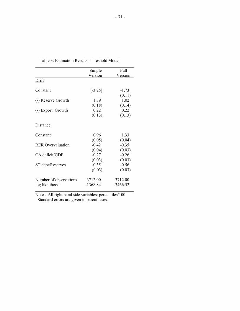
Table 3 shows the estimation results from the full model. (The results from the simple

version of the model are reproduced in the first column for comparison.) Coefficient estimates all

have the expected signs, and are highly significant except for export growth, which is again

marginally significant. The major difference between the full and the simple estimations is the larger

21 Using a similar methodology, the probit framework is a better fit for these data than the poisson model.

- 22 -

coefficient on short-term debt relative to reserves. All other coefficients (but the constant terms) are

very similar.

Consider first the estimates of distance from the threshold that would trigger a crisis (D/σ).

Recall that all explanatory variables are measured as percentiles/100, and range from 0 to 1.0. If all

three determinants of distance were at their lowest possible values, distance would be 1.33. If all

three variables were at their largest possible values, distance would be 0.16 = 1.33 � 0.35 � 0.26 �

0.56. Distance is most sensitive to changes in short-term debt relative to reserves. A 10 percentile

increase in this debt variable shrinks distance by more than twice a much as a 10 percentile rise in the

CA deficit/GDP, and by 60% more than a 10 percentile rise in real overvaluation.

Perhaps surprisingly, the coefficient estimates imply that drift is always negative in this

sample. The estimates for drift (δ/σ) range between �1.73 (when export and reserve declines are both

at their 0th percentiles) and �0.49 when both are at 100th percentiles. Drift is much more sensitive to

reserve growth than to export growth. A 10 percentile decline in reserve growth raises drift by more

than five times as much as a 10 percentile decline in export growth.22

Some general points can be made about the implications of these estimates. First, the

estimated possible values for both distance and drift are small relative to the standard deviation of

shocks, which is implicitly equal to one: σ = 1. This implies that shocks play an important role,

relative to trend factors, in determining the probable timing of a crisis. It also explains why there may

be sizable probabilities of crises, even though the underlying process is trending away from the

critical threshold. Second, with negative drift, there is a finite probability that no crisis will ever

occur: 1- Pr( T < ∞ ) = 1- exp( 2Dδ/ σ 2 ). This range of implied probabilities is computed below,

corresponding to all explanatory variables at the 0th, 50th or 100th percentiles:

Percentiles (D/σ) (δ/σ) Pr(T < ∞ ) Pr(never have a crisis)

0.0 1.33 -1.73 0.01 0.99

50.0 0.75 -1.11 0.19 0.81

100.0 0.16 -0.49 0.85 0.19

22 Recall that 24 months is defined as one period. If (D/F) = (δ/F) = 1.0, then the expected waiting time to a crisis would be 24 months.

- 23 -

These figures clearly illustrate the fact that there is a non-linear relationship between determinants of

distance and drift, and the probability of a crisis over different horizons. Thus, we turn next to look at

the evolution of the probability of a crisis within 3 months, 12 months and 24 months for selected

countries in the sample: Brazil, Indonesia, Korea, Mexico and Venezuela. These probabilities, as

well as the evolutions of distance and drift, are plotted in figures 4.a � 4.e.

7. Concluding Remarks

This paper has developed and applied a model of the timing of currency crises. The essence

of this model is that the timing of a crisis is determined by the first passage of an underlying process

through a threshold. If the process is Brownian motion, then the probability distribution of first

passage times can be shown to have an inverse gaussian distribution (IG). In this context, the IG

distribution is a very flexible function of two parameters: initial distance of the process from the

threshold and drift towards or away from the threshold, both relative to the standard deviation of

underlying shocks. This model can be derived from a first generation model of currency crisis, where

the underlying process is the shadow exchange rate. A threshold model can also be related to stylized

versions of second generation models. The specification is tractable, and provides a means of

estimating the probability of a crisis over any future time horizon, as a function of current indicators.

The threshold model is estimated on monthly data for 25 emerging market countries during

1995-98. Maximum likelihood estimation is used to study determinants of the probability of a crisis

within 24 months. This simple version of the model is shown to fit better than the popular but ad hoc

probit specification. (Indeed, it is shown that a probit specification is equivalent to imposing a series

of restrictions on the probability equationf from the threshold model.) It also out performs an

exponential distribution of first passage times, that comes from modeling crisis as a poisson process.

Estimation of the full model, using information about the month in which crises occurred,

produces sensible and interesting results. In particular, the most important indicator of distance is

short-term debt relative to reserves � a key variable in some second generation models of crisis. The

most important indicator of drift is the rate of change of foreign exchange reserves � a variable that is

central to the first generation models. Both distance and drift are estimated to be small relative to the

standard deviation of underlying shocks. And perhaps surprisingly, drift is always estimated to be

- 24 -

negative, so that the process is moving away from the threshold that would trigger a crisis. However,

this implies there is a finite probability that a crisis will never occur. Indeed, the probability of never

having a crisis ranges from 0.19 to 0.99. The model is also used to generate estimates of how of the

probabilities of a crisis over 3, 12 and 24 months evolved during the sample period.

There are a number of issues left for future work. First, it would be useful to formalize the

link between a version of the second generation crisis model and the threshold model developed here.

Second, it would be interesting to study more explicitly the appropriateness of specific theoretical

models of currency crises for understanding particular crisis episodes. Third, more work is required

on the sensitivity of the results to the definition of a crisis and to the scaling of explanatory variables.

Finally, an additional avenue to be explored is out-of-sample forecasting using the threshold model.

- 25 -

References

Abiad, Abdul 2003, �Early Warning Systems: A Survey and a Regime Switching Approach,� IMF Working Paper WP/03/32 (February). Agenor, Pierre-Richard, Jagdeep Bhandari and Robert Flood, 1992, �Speculative Attacks and Models of Balance-of-Payments Crises,� Staff Papers, Vol. 39, IMF, pp. 357-94. Berg, Andrew and Catherine Pattillo, 1999a, �Are Currency Crises Predictable? A Test,� IMF Staff Papers, Vol. 46, No. 2 (June) pp. 107-38. Berg, Andrew and Catherine Pattillo, 1999b, �Predicting Currency Crises: The Indicators Approach and an Alternative,� Journal of International Money and Finance, Vol. 18, No. 4, (August) pp. 561-586. Blackburn, Keith and Martin Sola,1993, �Speculative Currency Attacks and Balance of Payments Crises,� Journal of Economic Surveys, Vol. 7, No. 2, pp. 119-44. Blanco, Herminio and Peter Garber, 1986, �Recurrent Devaluation and Speculative Attacks on the Mexican Peso,� Journal of Political Economy, Vol. 94, No. 1. pp. 148-66 (February). Block, Steven, 2002, �Political Conditions and Currency Crises: Empirical Regularities in Emerging Markets,� Center for International Development, Harvard University Working Paper #79 (March). Borensztein, Edardo, Andrew Berg, Gian Maria Milesi-Ferretti and Catherine Pattillo, 2000, �Anticipating Balance of Payments Crises � the Role of Early Warning Systems,” IMF Occasional Paper #186. Bussiere, Mattieu and Marcel Fratzscher, 2002, �Towards a New Early Warning System of Financial Crises,� European Central Bank Working paper #145 (May). Chhikara, Raj S. and J. Leroy Folks, 1989, The Inverse Gaussian Distribution, New York: Marcel Dekker, Inc. Collins, Susan M., 1992, �The Expected Timing of EMS Realignments: 1979-83,� NBER Working Paper # 4068 (May). Cox, D.R. and H.D. Miller, 1995, The Theory of Stochastic Processes, Washington D.C.: Chapman & Hall/CRC. Cumby, Robert and Sweder van Wijnbergen, 1989, �Financial Policy and Speculative Runs with a Crawling Peg: Argentina 1979-1981 ,� Journal of International Economics, Vol. 27, Nos. 1-2, pp. 111-27 (August).

- 26 -

Drazen, Allan, 2000, �Interest Rate and Borrowing Defense Against Speculative Attack,� Paper prepared for the Carnegie-Rochester Conference Series on Public Policy, Pittsburgh, PA, November 19-20, 1999. Edison, Hali, 2000, �Do Indicators of Financial Crises Work? An Evaluation of Early Warning Systems,� Board of Governors of the Federal Reserve System, International Finance Discussion Paper # 675 (July). Edwards, Sebastian, 2002, �Does the Current Account Matter?� in S. Edwards and J. A. Frankel (eds.) Preventing Currency Crises in Emerging Markets, Chicago: NBER and Chicago University Press. Eichengreen, Barry, Andrew Rose and Charles Wyplosz, 1995, �Exchange Market Mayhem: The Antecedents and Aftermath of Speculative Attacks,� Economic Policy, Vol. 21, pp. 249-312. Eichengreen, Barry, Andrew Rose and Charles Wyplosz, 1996, �Speculative Attacks on Pegged Exchange Rates: An Empirical Exploration With Special Reference to the European Monetary System,� in M. Canzoneri, W. Ethier and V. Grilli (eds.) The New Transatlantic Economy, Cambridge: Cambridge University Press. Eichengreen, Barry and Olivier Jeanne, 2000, �Currency Crisis and Unemployment: Sterling in 1931,� in Paul Krugman (ed.) Currency Crises, Cambridge MA: NBER and University of Chicago, pp. 7-43. Esquivel, Gerardo and Felipe Larraín. 1998. �Explaining Currency Crises,� HIID, mimeo (November). Flood, Robert and Peter Garber, 1984, �Collapsing Exchange Rate Regimes: Some Linear Examples,� Journal of International Economics, Vol. 17, Nos. 1-2, pp. 1-13. Flood, Robert and Nancy Marion, 1997, �The Size and Timing of Devaluations in Capital-Controlled Developing Countries,� Journal of Development Economics, Vol. 54, No. 1, pp. 123-147.

Flood, Robert and Nancy Marion, 1999, �Perspectives on the Recent Currency Crisis Literature,� International Journal of Finance and Economics, Vol. 4, No. 1, pp. 1-26. Frankel, Jeffrey and Andrew Rose, 1996, �Currency Crashes in Emerging Markets: An Empirical Treatment,� Journal of International Economics, Vol. 41, Nos. 3-4, pp. 351-66. Garber, Peter and Lars Svensson, 1995, �The Operation and Collapse of Fixed Exchange Rate Regimes,� in , G. Grossman and K. Rogoff (eds).Handbook of International Economics, Vol. 3, North Holland, Amsterdam, pp. 1865-1911.

Goldberg, Linda, 1994, �Predicting Exchange Rate Crises: Mexico Revisited,� Journal of International Economics, Vol. 36, Nos. 3-4, pp.413-30. Goldfajn, Ilan and Rodrigo Valdes, 1997, �Are Currency Crises Predictable?� IMF Working Paper WP/97/159 (December).

- 27 -

Jeanne, Olivier, 2000, Currency Crises: A Perspective on Recent Theoretical Developments, Special Papers in International Economics, Princeton University, No. 20 (March). Jeanne, Olivier and Paul Masson, 2000, �Currency Crises, Sunspots and Markov Switching Regimes,� Journal of International Economics, Vol. 50, No. 2 (April) pp. 327-50. Kamin, Steven B., John W. Schindler, and Shawna L. Samuel, 2001, "The Contribution of Domestic and External Factors to Emerging Market Devaluation Crises: An Early Warning Systems Approach," International Finance Discussion Papers 711, Board of Governors of the Federal Reserve System (U.S.) Kaminsky, Graciela, Saul Lizondo and Carmen Reinhart, 1998, �Leading Indicators of Currency Crises,� Staff Papers, Vol. 45, No. 1,Washington DC: International Monetary Fund, pp. 1-48 (March). Kaminsky, Graciela, 1998, �Currency and Banking Crises: The Early Warnings of Distress,� International Finance Discussion Papers 629, Board of Governors of the Federal Reserve System (U.S.) Kaminsky, Graciela and Carmen Reinhart, 1999, �The Twin Crises: The Causes of Banking and Balance-of-Payments Problems,� American Economic Review, Vol. 89, No. 3, pp. 473-500. Klein, Michael and Nancy Marion, 1997, �Explaining the Duration of Exchange Rate Pegs,� Journal of Development Economics, Vol. 54, pp. 387-404. Krugman, Paul, 1979, �A Model of Balance of Payments Crises,� Journal of Money, Credit and Banking, Vol. 11, No. 3, pp. 311-25. Krugman, Paul, 1996, �Are Currency Crises Self-Fulfilling?� in Ben Bernanke and Julio Rotemberg (eds.) NBER Macroeconomics Annual, Cambridge MA: MIT Press, pp. 345-78. Kumar, Mohan, Uma Moorthy and William Perraudin, 2002, �Predicting Emerging Market Currency Crashes,� IMF Working Paper 02/07, International Monetary Fund, Washignton, DC. Martinez-Peria, Maria Soledad, 2002, �A Regime Switching Approach to Studying Speculative Attacks: A Focus on EMS Crises,� Empirical Economics, Vol. 27, No. 2, pp. 299-334. Milesi-Ferretti, Gian Maria and Assaf Razin, �Current Account Reversals and Currency Crises: Empirical Regularities,� in Paul Krugman (ed.) Currency Crises, Cambridge MA: NBER and University of Chicago, pp. 285-323. Mulder, Christian B., Perrelli, Roberto, Rocha, Manuel. 2002. �The Role of Corporate, Legal and Macroeconomic Balance Sheet Indicators in Crisis Detection and Prevention.� Working Paper No. 02/59, International Monetary Fund (March). Obstfeld, Maurice, 1995, �The Logic of Currency Crises,� in Barry Eichengreen, Jeffry Frieden, and Jurgen von Hagen (eds.) Monetary and fiscal policy in an integrated Europe. European and Transatlantic Studies. Heidelberg; New York and London: Springer, pp. 62-90

- 28 -

Obstfeld, Maurice, 1996, �Models of Currency Crises with Self-Fulfilling Features,� European Economic Review, Vol. 40, Nos. 3-5, pp. 1037-48. Obstfeld, Maurice and Kenneth Rogoff, 1995, �The Mirage of Fixed Exchange Rates,� Journal of Economic Perspectives, Vol. 9, No. 4 (Fall) pp. 73-96. Rodrik, Dani and Andrés Velasco, 1999, �Short-Term Capital Flows,� NBER Working Paper #7364 (September). Sachs, Jeffrey, Aaron Tornell and Andrés Velasco, 1996, �Financial Crises in Emerging Markets: The Lessons from 1995,� Brookings papers on Economic Activity, No. 1, pp. 147-215. Salant, Stephen and Dale Henderson, 1978, �Market Anticipations of Government Policies and the Price of Gold,� Journal of Political Economy, Vol. 86, No. 4, pp. 627-48. Tornell, Aaron, 1999, �Common Fundamentals in the Tequila and Asian Crises,� NBER Working Paper #7139. Tudela, Mar a Mercedes, 2001, �Explaining Currency Crises: A Duration Model Approach,� Centre for Economic Performance, London School of Economics and Political Science, Working Paper (January). Vlaar, Peter, 2000, �Early Warning Systems for Currency Crises,� Papers 671, De Nederlandsche Bank.

- 29 -

Table 1. Countries and Crisis Dates: 1985-98

Countries Crisis Dates 1 Argentina 1989:04, 1990:02 2 Bolivia none 3 Brazil 1990:11, 1991:10 4 Chile none 5 Columbia 1995:08, 1998:09 6 Cyprus 1991:03 7 Egypt 1990:07, 1991:03 8 India 1991:04, 1991:07, 1993:03 9 Indonesia 1986:09, 1998:01, 1998:06 10 Israel none 11 Jordan 1988:04, 1988:06, 1988:10, 1989:02 12 Korea 1997:11, 1997:12 13 Lebanon 1990:08 14 Malaysia 1997:07, 1997:08, 1997:12, 1998:01 15 Mexico 1994:12 16 Pakistan none 17 Peru 1987:10, 1987:12 18 Philippines 1986:02, 1997:12 19 South Africa none 20 Sri Lanka none 21 Thailand 1997:07, 1997:08, 1997:12, 1998:01 22 Turkey 1994:03, 1994:04 23 Uruguay none 24 Venezuela 1986:12, 1989:03, 1994:05, 1995:12, 1996:04 25 Zimbabwe 1991:09, 1997:11, 1998:08

- 30 -

Table 2. Estimation Results: Probability of crisis within 24 months Simple Simple Threshold Threshold Simple Poisson Probit Model Model Threshold Model Model Drift=0 Drift=const. Model

Distance Distance Distance

Constant: -0.28 -3.25 3.20 2.42 0.96 (0.02) (0.12) (0.09) (0.55) (0.05) RER Overvaluation 0.27 1.35 -1.06 -0.85 -0.42 (0.02) (0.10) (0.07) (0.18) (0.04) CA deficit/GDP 0.15 0.71 -0.61 -0.53 -0.27 (0.03) (0.11) (0.08) (0.11) (0.03) ST debt/Reserves 0.37 1.29 -0.98 -0.75 -0.35 (0.03) (0.11) (0.86) (0.18) (0.03) Drift (-) Reserve Growth 0.19 0.72 -0.54 -0.41 1.39 (0.02) (0.11) (0.09) (0.11) (0.18) (-) Export Growth 0.00 0.24 -0.20 -0.15 0.39

(0.02) (0.11) (0.08) (0.07) (0.19) Drift Drift Constant -- -- [0.00] -0.63 [-3.25] (0.44) Number of observations 3712 3712 3712 3712 3712 log likelihood -1389.38 -1378.88 -1375.34 -1374.46 -1368.84 Notes: All right hand side variables: percentiles/100. Standard errors are given in parentheses. The probit model is equivalent to the threshold (inverse gaussian) model with drift=0 and the second

term omitted (see text). The distinction between distance and drift is only relevant for the threshold model.

- 31 -

Table 3. Estimation Results: Threshold Model Simple Full Version Version Drift Constant [-3.25] -1.73 (0.11) (-) Reserve Growth 1.39 1.02 (0.18) (0.14) (-) Export Growth 0.22 0.22 (0.13) (0.13) Distance Constant 0.96 1.33 (0.05) (0.04) RER Overvaluation -0.42 -0.35 (0.04) (0.03) CA deficit/GDP -0.27 -0.26 (0.03) (0.03) ST debt/Reserves -0.35 -0.56

(0.03) (0.03)

Number of observations 3712.00 3712.00 log likelihood -1368.84 -3466.52 Notes: All right hand side variables: percentiles/100. Standard errors are given in parentheses.