probability and statistics nasa

NASA / TP--1998-207194

Probability and Statistics in Aerospace

EngineeringM.H. Rheinfurth and L.W. Howell

Marshall Space Flight Center, Marshall Space Flight Center, Alabama

National Aeronautics and

Space Administration

Marshall Space Flight Center

March 1998

NASA Center for AeroSpace Information

800 Elkridge Landing Road

Linthicum Heights, MD 21090-2934

(301) 621-0390

Available from:

ii

National Technical Information Service

5285 Port Royal Road

Springfield, VA 22161

(703) 487-4650

TABLE OF CONTENTS

I. INTRODUCTION ..................................................................................................................... 1

A. Preliminary Remarks ........................................................................................................ 1

B. Statistical Potpourri .......................................................................................................... 1

C. Measurement Scales ......................................................................................................... 2

D. Probability and Set Theory ............................................................................................... 2

II. PROBABILITY ......................................................................................................................... 5

A. Definitions of Probability ................................................................................................. 5

B. Combinatorial Analysis (Counting Techniques) ............................................................... 6

C. Basic Laws of Probability ................................................................................................ 10

D. Probability Distributions .................................................................................................. 19

E. Distribution (Population) Parameters ............................................................................... 23

F. Chebyshev's Theorem ...................................................................................................... 26

G. Special Discrete Probability Functions ............................................................................. 27

H. Special Continuous Distributions ..................................................................................... 32

I. Joint Distribution Functions ............................................................................................. 41

J. Mathematical Expectation ................................................................................................ 48K. Functions of Random Variables ........................................................................................ 50

L. Central Limit Theorem (Normal Convergence Theorem) ................................................ 61

M. Simulation (Monte Carlo Methods) .................................................................................. 61

IH. STATISTICS .............................................................................................................................. 64

A. Estimation Theory ............................................................................................................ 64B. Point Estimation ............................................................................................................... 65

C. Sampling Distributions ..................................................................................................... 74

D. Interval Estimation ........................................................................................................... 79

E. Tolerance Limits ............................................................................................................... 83

E Hypothesis/Significance Testing ...................................................................................... 85

G. Curve Fitting, Regression, and Correlation ...................................................................... 91H. Goodness-of-Fit Tests ....................................................................................................... 103

I. Quality Control ................................................................................................................. 107

J. Reliability and Life Testing .............................................................................................. 112

K. Error Propagation Law ..................................................................................................... 118

BIBLIOGRAPHY ................................................................................................................................. 124

iii

LIST OF FIGURES

,

2.

3.

4.

5.

o

7.

8.

9.

10.

11.

12.

13.

14.

15.

16.

17.

18.

19.

20.

21.

22.

23.

24.

25.

26.

27.

28.

29.

30.

31.

Venn diagram ............................................................................................................................. 11

Conditional probability .............................................................................................................. 11

Partitioned sample space ........................................................................................................... 15

Bayes' Rule ................................................................................................................................ 15

Cartesian product ....................................................................................................................... 19

Function A _ B .......................................................................................................................... 20

Coin-tossing experiment ............................................................................................................ 21

Probability function diagram ..................................................................................................... 21

Cumulative distribution function ............................................................................................... 22

Location of mean, median, and mode ........................................................................................ 24

Chebyshev's theorem ................................................................................................................. 26

Normal distribution areas: two-sided tolerance limits ............................................................... 33

Normal distribution areas: one-sided tolerance limits ............................................................... 34

Uniform p.d.f ............................................................................................................................. 37

Examples of standardized beta distribution ............................................................................... 39

Gamma distribution ................................................................................................................... 39

Cantilever beam ......................................................................................................................... 42

Posterior distribution with no failures ....................................................................................... 46

Two tests and one failure ........................................................................................................... 46

Lower confidence limit .............................................................................................................. 47

A function of a random variable ................................................................................................ 51

Random sine wave ..................................................................................................................... 52

Probability density of random sine wave .................................................................................. 53

Probability integral transformation ............................................................................................ 54

Sum of two random variables .................................................................................................... 57

Difference of two random variables .......................................................................................... 58

Interference random variable ..................................................................................................... 59

Buffon's needle .......................................................................................................................... 62

Area ratio of Buffon's needle .................................................................................................... 62

Sampling distribution of biased and unbiased estimator ........................................................... 67

Estimator bias as a function of parameter ................................................................................. 69

V

32.

33.

34.

35.

36.

37.

38.

39.

40.

41.

42.

43.

44.

45.

46.

47.

48.

49.

50.

51.

Population and sampling distribution ........................................................................................ 75

Student versus normal distribution ............................................................................................ 76

Z 2 distribution ............................................................................................................................ 77

Confidence interval for mean .................................................................................................... 80

Confidence interval for variance ............................................................................................... 81

One-sided upper tolerance limit ................................................................................................ 84

Two-sided tolerance limits ......................................................................................................... 85

Hypothesis test (H0 : bt =/20 HI :/.t = #1) .................................................................................. 87

Operating characteristic curve ................................................................................................... 89

One-sided hypothesis test .......................................................................................................... 90

Two-sided hypothesis test .......................................................................................................... 90

Significance test (a = 0.05) ...................................................................................................... 91

Linear regression line ................................................................................................................ 92

Prediction limits of linear regression ......................................................................................... 95

Nonintercept linear regression model ........................................................................................ 95

Sample correlation coefficient (scattergrams) ........................................................................... 98

Positive versus negative correlations ......................................................................................... 101

Quadratic relationship with zero correlation ............................................................................. 102

Kolmogorov-Smirnov test ......................................................................................................... 106

OC curve for a single sampling plan ......................................................................................... 109

vi

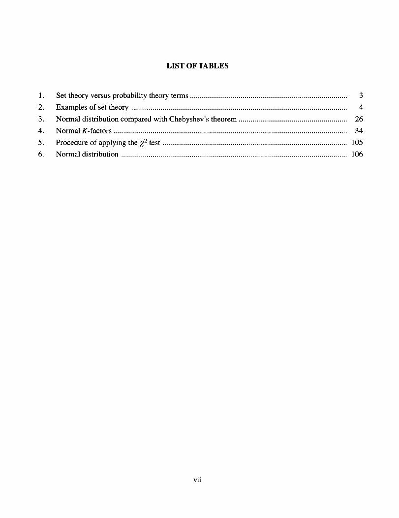
LIST OF TABLES

.

2.

3.

4.

5.

6.

Set theory versus probability theory terms ................................................................................ 3

Examples of set theory .............................................................................................................. 4

Normal distribution compared with Chebyshev's theorem ....................................................... 26

Normal K-factors ....................................................................................................................... 34

Procedure of applying the Z 2 test .............................................................................................. 105

Normal distribution ................................................................................................................... 106

vii

TECHNICAL PUBLICATION

PROBABILITY AND STATISTICS IN AEROSPACE ENGINEERING

I. INTRODUCTION

A. Preliminary Remarks

Statistics is the science of the collection, organization, analysis, and interpretation of numericaldata, especially the analysis of population characteristics by inference from sampling. In engineering workthis includes such different tasks as predicting the reliability of space launch vehicles and subsystems, life-time analysis of spacecraft system components, failure analysis, and tolerance limits.

A common engineering definition of statistics states that statistics is the science of guidingdecisions in the face of uncertainties. An earlier definition was statistics is the science of making decisionsin the face of uncertainties, but the verb making has been moderated to guiding.

Statistical procedures can vary from the drawing and assessment of a few simple graphs to carry-ing out very complex mathematical analysis with the use of computers; in any application, however, thereis the essential underlying influence of "chance." Whether some natural phenomenon is being observed ora scientific experiment is being carried out, the analysis will be statistical if it is impossible to predict thedata exactly with certainty.

The theory of probability had, strangely enough, a clearly recognizable and rather definitive start. Itoccurred in France in 1654. The French nobleman Chevalier de Mere had reasoned falsely that the prob-ability of getting at least one six with 4 throws of a single die was the same as the probability of getting atleast one "double six" in 24 throws of a pair of dice. This misconception gave rise to a correspondencebetween the French mathematician Blaise Pascal (1623-1662) and his mathematician friend Pierre Fermat

(1601-1665) to whom he wrote: "Monsieur le Chevalier de Mere is very bright, but he is not a mathe-matician, and that, as you know, is a very serious defect."

B. Statistical Potpourri

This section is a collection of aphorisms concerning the nature and concepts of probability andstatistics. Some are serious, while others are on the lighter side.

"The theory of probability is at bottom only common sense reduced to calculation; it makes usappreciate with exactitude what reasonable minds feel by a sort of instinct, often without being able toaccount for it. It is remarkable that this science, which originated in the consideration of games of chance,should have become the most important object of human knowledge." (P.S. Laplace, 1749-1827)

"Statistical thinking will one day be as necessary for efficient citizenship as the ability to readand write." (H.G. Wells, 1946)

From a file in the NASA archiveson "Humor and Satire:" Statistics is a highly logical and

precise method of saying a half-truth inaccurately.

A statistician is a person who constitutionally cannot make up his mind about anything and underpressure can produce any conclusion you desire from the data.

There are three kinds of lies: white lies, which are justifiable; common lies, which have nojustification; and statistics.

From a NASA handbook on shuttle launch loads: "The total load will be obtained in a rational

manner or by statistical analysis."

Lotteries hold a great fascination for statisticians, because they cannot figure out why people playthem, given the odds.

There is no such thing as a good statistical analysis of data about which we know absolutelynothing.

Real-world statistical problems are almost never as clear-cut and well packaged as they appearin textbooks.

Statistics is no substitute for good judgment.

The probability of an event depends on our state of knowledge (information) and not on the state ofthe real world. Corollary: There is no such thing as the "intrinsic" probability of an event.

C. Measurement Scales

The types of measurements are usually called measurement scales. There exist four kindsof scales. The list proceeds from the "weakest" to the "strongest" scale and gives an example of each:

• Nominal Scale: Red, Green, Blue• Ordinal Scale: First, Second, Third• Interval Scale: Temperature• Ratio Scale: Length.

Most of the nonparametfic (distribution-free) statistical methods work with interval or ratio scales.In fact, all statistical methods requiring only a weaker scale may also be used with a stronger scale.

D. Probability and Set Theory

The formulation of modem probability theory is based upon a few fundamental concepts of settheory. However, in probability theory these concepts are expressed in a language particularly adapted toprobability terminology. In order to relate the notation commonly used in probability theory to that of settheory, we first present a juxtaposition of corresponding terms, shown in table 1.

2

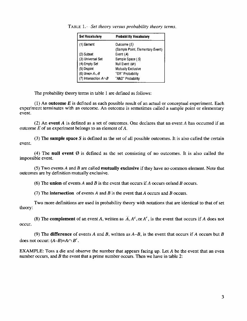
TABLE 1.--Set theory versus probability theory terms.

SelVocabulary ProbabilityVocabulary

(1)Element Outcome(E)(SamplePoint,ElementaryEvent)

(2)Subset Event(A)(3)UniversalSet SampleSpace(5)(4)EmptySet NullEvent(_)(5)Disjoint MutuallyExclusive(6)UnionAuB "OR"Probability(7) IntersectionAc_B "AND"Probability

The probability theory terms in table 1 are defined as follows:

(1) An outcome E is defined as each possible result of an actual or conceptual experiment. Eachexperiment terminates with an outcome. An outcome is sometimes called a sample point or elementaryevent.

(2) An event A is defined as a set of outcomes. One declares that an event A has occurred if an

outcome E of an experiment belongs to an element of A.

(3) The sample space S is defined as the set of all possible outcomes. It is also called the certainevent.

(4) The null event 0 is defined as the set consisting of no outcomes. It is also called theimpossible event.

(5) Two events A and B are called mutually exclusive if they have no common element. Note thatoutcomes are by def'mition mutually exclusive.

(6) The union of events A and B is the event that occurs if A occurs or/and B occurs.

(7) The intersection of events A and B is the event that A occurs and B occurs.

Two more definitions are used in probability theory with notations that are identical to that of settheory:

occur.

(8) The complement of an event A, written as A, A c, orA', is the event that occurs if A does not

(9) The difference of events A and B, written as A-B, is the event that occurs if A occurs but B

does not occur: (A-B)=An B'.

EXAMPLE: Toss a die and observe the number that appears facing up. Let A be the event that an evennumber occurs, and B the event that a prime number occurs. Then we have in table 2:

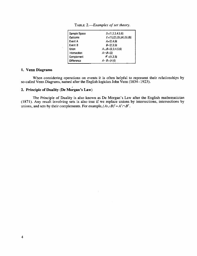
TABLE2.--Examplesof set theory.

SampleSpace S={1,2,3,4,5,6}Outcome E={1},{2},{3},{4},{5},{6}EventA A={2,4,6}EventB B={2,3,5}Union A_JB={2,3,4,5,6}Intersection AnB={2}Complement A'={1,3,5}Difference A- B= {4,6}

1. Venn Diagrams

When considering operations on events it is often helpful to represent their relationships byso-called Venn Diagrams, named after the English logician John Venn (1834-1923).

2. Principle of Duality (De Morgan's Law)

The Principle of Duality is also known as De Morgan's Law after the English mathematician(1871). Any result involving sets is also true if we replace unions by intersections, intersections by

unions, and sets by their complements. For example, (AuB)" =A'_B'.

4

II. PROBABILITY

A. Definitions of Probability

1. Classical (a Priori) Definition

The classical (a priori) definition of probability theory was introduced by the French mathe-

matician Pierre Simon Laplace in 1812. He defined the probability of an event A as the ratio of thefavorable outcomes to the total number of possible outcomes, provided they are equally likely (probable):

P(A):_ (1)

where n=number of favorable outcomes and N=number of possible outcomes.

2. Empirical (a Posteriori) Definition

The empirical (a posteriori) definition was introduced by the German mathematician Richard V.

Mises in 1936. In this definition, an experiment is repeated M times and if the event A occurs re(A) times,then the probability of the event is defined as:

P(A)= lirn re(A)M---_ M (2)

Empirical Frequency. This definition of probability is sometimes referred to as the relative

frequency. Both the classical and the empirical definitions have serious difficulties. The classical definitionis clearly circular because we are essentially defining probability in terms of itself. The empirical definitionis unsatisfactory because it requires the number of observations to be infinite; however, it is quite useful inpractice and has considerable intuitive appeal. Because of these difficulties, statisticians now prefer theaxiomatic approach based on set theory.

3. Axiomatic Definition

The axiomatic definition was introduced by the Russian mathematician A.N. Kolmogorov in1933:

• Axiom 1: P(A)>O

• Axiom 2: P(S)=I

• Axiom 3: P(AwB)=P(A)+P(B) if A_B=O .

It follows from these axioms that for any event A, then:

0_<P(A)___I (3)

5

Probabilities and Odds. If the probability of event A is p, then the odds that it will occur are

given by the ratio ofp to 1-p. Odds are usually given as a ratio of two positive integers having no com-

mon factors. If an event is more likely to not occur than to occur, it is customary to give the odds that itwill not occur rather than the odds that it will occur.

EXAMPLE:

• Probability: P=A/B where A and B are any two positive numbers and A<_B.

Odds: A: (B-A).

If the probability of an event is p=3/4, we say that the odds are 3:1 in its favor.

• Given the odds are A to B, then the probability is A/(A+B).

Criticality Number. For high reliability systems it is often preferable to work with the probability

of failure multiplied by 106. This is called the criticality number. For instance, if the system has a

probability of success of P=0.9999, then the criticality number is C=100.

B. Combinatorial Analysis (Counting Techniques)

In obtaining probabilities using the classical definition, the enumeration of outcomes often becomespractically impossible. In such cases use is made of combinatorial analysis, which is a sophisticated wayof counting.

la Permutations

A permutation is an ordered selection of k objects from a set S having n elements.

• Permutations without repetition:

k)=nP k =n×(n-1)×(n-2)...(n-k +l)= (nn-_/k)!_.Po(n,

• Permutations with repetition:

P 1(n, k)=n k

(4)

(5)

Combinations

A combination is an unordered selection of k objects from a set S having n elements.

• Combinations without repetition:

Co(n,k)=nCk =(_ ) n!= k!(n-k)! (called "binomial coefficient") . (6)

• Combinationswith repetition:

C "nk' fn+k-l'_ (n+k-1)!lt, )=_ k )=k/(n-1)/

EXAMPLES: Selection of two letters from {a, b, c }:

(1) P0(n,k)=P0 (3, 2)=3x2=6

ab, ac, ba, be, ca, cb

(2) Pl(n,k)=Pl(3,2)=3x3=9

aa, ab, ac, ba, bb, be, ca, cb, cc

(3) Co(n, k)=C0 (3, 9_- 3x2_a-J- lx2 -_

ab, ac, bc

(4) Cl(n, k)=Cl (3, 9_- 3x4_¢_

aa, bb, cc, ab, ac, bc

Without repetition

With repetition

Without repetition

With repetition

(7)

PROBLEM: Baskin-Robbins ice-cream parlors advertise 31 different flavors of ice cream. What is thenumber of possible triple-scoop cones without repetition, depending on whether we are interested in howthe flavors are arranged or not?

SOLUTION: 31P3=26,970 and 31C3=4,495.

3. Permutations of a Partitioned Set

Suppose a set consists of n elements of which nl are of one kind, n2 are of a second kind .... nk

are of a k th type. Here, of course, n=nl+n2+...nk. Then the number of permutations is:

P2(n, nk ) = n!nl !n 2 in 3 ! . . .nk ! (8)

An excellent reference for combinatorial methods is M. Hall's book Combinatorial Analysis.

PROBLEM: Poker is a game played with a deck of 52 cards consisting of four suits (spades, clubs,hearts, and diamonds) each of which contains 13 cards (denominations 2, 3, 4, 5, 6, 7, 8, 9, 10, J, Q, K,and A.) When considered sequentially, the A may be taken to be 1 or A but not both; that is, 10, J, Q, K,A is a five-card sequence called a "straight," as is A, 2, 3, 4, 5; but Q, K, A, 2, 3 is not sequential, that is,not a "straight."

A poker hand consists of five cards chosen at random. A winning poker hand is the one witha higher "rank" than all the other hands.

7

A "flush" is a five-card hand all of the same suit. A "pair" consists of two, and only two, cards of

the same kind, for example (js, jc). "Three-of-a-kind" and "four-of-a-kind" are defined similarly. A "fullhouse" is a five-card hand consisting of a "pair" and "three-of-a-kind." The ranks of the various hands areas follows with the highest rank first:

• Royal flush (10, J, Q, K, A of one suit)• Straight flush (consecutive sequence of one suit that is not a royal flush)• Four-of-a-kind• Full house

• Flush (not a straight flush)• Straight• Three-of-a-kind (not a full house)• Two pairs (not four of a kind)• One pair• No pair ("bust").

(1) Show that the number of possible poker hands is 2,598,960.

(2) Show that the number of possible ways to deal the various hands are:

(a) 4 (b) 36 (c) 624 (d) 3,744 (e) 5,108(f) 10,200 (g) 54,912 (h) 123,552 (i) 1,098,240 (j) 1,302,540

SOLUTIONS: Poker is a card game with a deck of 52 cards consisting of four suits (spades, clubs,hearts, and diamonds). Each suit contains 13 denominations (2, 3, 4, 5, 6, 7, 8, 9, 10, J, Q, K, and A).A poker hand has five cards and the players bet on the ranks of their hands. The number of possible waysto obtain each of these ranks can be determined by combinatorial analysis as follows:

(a) Royal Flush. This is the hand consisting of the 10, J, Q, K, and A of one suit. There are fourof these, one for each suit, and hence, N=4.

(b) Straight Flush. All five cards are of the same suit and in sequence, such as the 6, 7, 8, 9, and10 of diamonds. Their total number is 10 for each suit. However, we have to exclude the four royal

flushes contained in this set. Therefore, the total number of straight flushes is N=10x4-4=36.

(c) Four-of-a-Kind. This hand contains four cards of the same denomination such as four aces orfour sixes and then a fifth unmatched card. The total number of possible ways to choose this rank isobtained by:

(1) Choosing the denomination, 13 ways.

(2) Choosing the suit, 4 ways.

(3) Choosing the remaining unmatched card, 12 ways.

The result is: N=13x4x 12=624.

(d) Full House. This hand consists of three cards of one denomination and two cards of another,as 8-8-8-K-K. The total number of possible ways is given by the following sequence of selections:

(1) Choosing denomination of the first triplet of cards, 13 ways.

8

_2_Selecting_eeoutof_efoursuits_or_is_plet(4)4ways(3) Choosing the denomination of the second doublet of cards, 12 ways.

(4) Selecting two out of the four suits for this doublet, (4)=6 ways.

The result is then N=13x4×12x6=3,744.

(e) Flush. This hand contains five cards of the same suit, but not all in sequence. To obtain the

number of possible ways, select 5 out of 13 denominations, (13)=1,287 ways, and select one of the four

suits, 4 ways for a total ofN=1,287x4 =5,148. Here we have to consider again that this number contains

the number of straight flushes and royal flushes which have to be subtracted from it. The result is

N=5,148-36-4=5,108.

(f) Straight. This hand contains a five-card sequence as defined above. We observe that there are10 possible five-card sequences. Each face value in this sequence can come from any of the four denomi-

nations, which results in 45 different ways of creating a particular five-card sequence. The result is:

N=10x45=10,240. Again, it must be noted that this number contains the number of straight flushes and

royal flushes which have to be subtracted for the final answer: N=10,240-36-4=10,200.

(g) Three-of-a-Kind. This hand contains three cards of one denomination and two different cards,each of different denominations. The total number of ways is obtained by:

(1) Choose the denomination of the three cards, 13 ways.

(2) Select three of the four suits in 4 ways.

Select 2 of the remaining 12 denominations (1_)=66(3) ways.

(4) Each of the two remaining cards can have any of the four denominations for 4x4=16.

The total number for this rank is, therefore, N=13x4x66x16=54,912.

(h) Two Pairs. To obtain the number of possible ways for this rank, we take the following steps:

,1,Select_e_eno=a.onof_otwo._s_n('_)_8ways

_2,Sol_t_etwosuitsforeachpa__(4)=36ways(3) Select the denomination of the remaining card. There are 11 face values left.

(4) The remaining card can have any of the four suits.

9

Thetotal numberis, therefore,N=78x36xl lx4=123,552.

(i) One Pair. The number of possible ways for this rank is obtained according to the following steps:

(1) Select denomination of the pair in 13 ways.

(2) Select suit in (4)=6 ways.

(3) Select denomination of the other three cards from the remaining 12 denominations

in (_2)=220 ways.

(4) Each of these three cards can have any suit, resulting in 43=64 ways.

The total number is then N= 13x6x220x64 = 1,098,240.

(j) No Pair. The number of ways for this "bust" rank is obtained according to the following steps:

Select five cards from 13 denominations as (153)=1,287.(1)

(2) Each card can have any suit, giving 45=1,024.

The result is N=1,287×1,024=1,317,888. Again, we note that this number contains the number

of royal flushes, straight flushes, flushes, and straights. Thus, we obtain as the answer:

N=l,317,888-4-36-5,108-10,200=1,302,540 .

QUESTION: The Florida State Lottery requires the player to choose 6 numbers without replacement froma possible 49 numbers ranging from 1 to 49. What is the probability of choosing a winning set of num-bers? Why do people think a lottery with the numbers 2, 13, 17, 20, 29, 36 is better than the one with thenumbers 1,2, 3, 4, 5, 6? (Hint: use hypergeometric distribution.)

C. Basic Laws of Probability

1. Addition Law ("OR" Law; "AND/OR")

The Addition Law of probability is expressed as:

P(A_B) = P(A)+P(B)-P(AnB) (9)

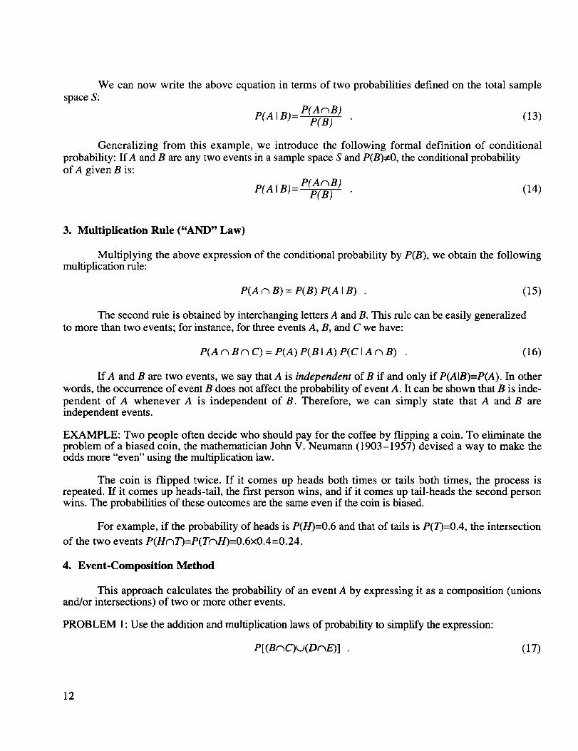
The Venn diagram in figure 1 is helpful in understanding this probability law. A formal proof can

be found in any standard textbook. In Venn diagrams, the universal set S is depicted by a rectangle and thesets under consideration by closed contours such as circles and ellipses.

10

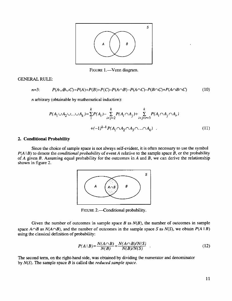
FIGURE 1.--Venn diagram.

GENERAL RULE:

n=3: P(A_BuC) =P(A)+P(B)+P(C)-P(AnB)-P(AnC)-P(BnC)+P(AnBnC)

n arbitrary (obtainable by mathematical induction):

k k k

P(AIUA2_...UAk)=]_P(Ai )- ]_ P(AinAj)+ Y_ P(A_nAj_A r)1 i<j=2 i<j<r=-3

(10)

+(-1) k-1 P(A 1n A 2 n A 3 n... n Ak) (11)

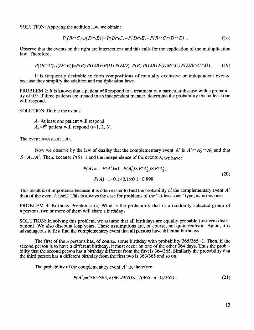
2. Conditional Probability

Since the choice of sample space is not always self-evident, it is often necessary to use the symbolP(A IB) to denote the conditional probability of event A relative to the sample space B, or the probability

of A given B. Assuming equal probability for the outcomes in A and B, we can derive the relationshipshown in figure 2.

FIGURE 2.---Conditional probability.

Given the number of outcomes in sample space B as N(B), the number of outcomes in sample

space AcaB as N(AnB), and the number of outcomes in the sample space S as N(S), we obtain P(A IB)

using the classical definition of probability:

P(A IB)= N(AnB) _ N(AcaB)/N(S) (12)N(B) N(B)/N(S)

The second term, on the right-hand side, was obtained by dividing the numerator and denominator

by N(S). The sample space B is called the reduced sample space.

11

We cannow write the aboveequationin termsof two probabilitiesdefinedon the total samplespaceS:

P(AAB)P(AIB)= P(B) (13)

Generalizing from this example, we introduce the following formal definition of conditional

probability: If A and B are any two events in a sample space S and P(B)¢-O, the conditional probability

of A given B is:

P(AnB)P(AIB)= P(B) (14)

3. Multiplication Rule ("AND" Law)

Multiplying the above expression of the conditional probability by P(B), we obtain the followingmultiplication rule:

P( A n B) = P( B) P( A I B) (15)

The second rule is obtained by interchanging letters A and B. This rule can be easily generalizedto more than two events; for instance, for three events A, B, and C we have:

P(A n B n C) = P(A) P(B IA) P(C IA n B) (16)

IrA and B are two events, we say that A is independent of B if and only if P(AIB)=P(A). In other

words, the occurrence of event B does not affect the probability of event A. It can be shown that B is inde-

pendent of A whenever A is independent of B. Therefore, we can simply state that A and B areindependent events.

EXAMPLE: Two people often decide who should pay for the coffee by flipping a coin. To eliminate theproblem of a biased coin, the mathematician John V. Neumann (1903-1957) devised a way to make theodds more "even" using the multiplication law.

The coin is flipped twice. If it comes up heads both times or tails both times, the process isrepeated. If it comes up heads-tail, the fh'st person wins, and if it comes up tail-heads the second personwins. The probabilities of these outcomes are the same even if the coin is biased.

For example, if the probability of heads is P(H)=0.6 and that of tails is P(T)=0.4, the intersection

of the two events P(HnT)=P(TnH)=0.6×0.4=0.24.

4. Event-Composition Method

This approach calculates the probability of an event A by expressing it as a composition (unionsand/or intersections) of two or more other events.

PROBLEM 1: Use the addition and multiplication laws of probability to simplify the expression:

P[(BAC)u(DAE)] (17)

12

SOLUTION:Applyingtheadditionlaw,weobtain:

P[ ( Bn C) t..)(D_ E)] = P( Bn C)+ P( D_ E)- P( Bn Cn Dn E) (18)

Observe that the events on the right are intersections and this calls for the application of the multiplicationlaw. Therefore,

P[(BnC)u(D_E)]=P(B) P(CIB)+P(D) P(EID)-P(B) P(CIB) P(DIBnC) P(EIBnCnD) . (19)

It is frequently desirable to form compositions of mutually exclusive or independent events,because they simplify the addition and multiplication laws.

PROBLEM 2: It is known that a patient will respond to a treatment of a particular disease with a probabil-ity of 0.9. If three patients are treated in an independent manner, determine the probability that at least onewill respond.

SOLUTION: Define the events:

A=At least one patient will respond.

Ai=i th patient will respond (i=1, 2, 3).

The event A=A1uA2t..)A3 .

Now we observe by the law of duality that the complementary event A' is A[nA_ nA_ and that

S=AuA'. Then, because P(S)=I and the independence of the events Ai we have:

P(A) = l- P(A') = 1- P(A{ )x P(A_ ) x P(A_ )

P(A)=I-O. lxO. lxO. 1 =0.999.(20)

This result is of importance because it is often easier to find the probability of the complementary event A'

than of the event A itself. This is always the case for problems of the "at-least-one" type, as is this one.

PROBLEM 3: Birthday Problems: (a) What is the probability that in a randomly selected group of

n persons, two or more of them will share a birthday?

SOLUTION: In solving this problem, we assume that all birthdays are equally probable (uniform distri-bution). We also discount leap years. These assumptions are, of course, not quite realistic. Again, it isadvantageous to first find the complementary event that all persons have different birthdays.

The first of the n persons has, of course, some birthday with probability 365/365=1. Then, if thesecond person is to have a different birthday, it must occur on one of the other 364 days. Thus the proba-bility that the second person has a birthday different from the fn'st is 364/365. Similarly the probability thatthe third person has a different birthday from the first two is 363/365 and so on.

The probability of the complementary event A' is, therefore:

P( A ") = (365/365)x(364/365)×...((365-n+1)/365) . (21)

13

Thedesiredprobabilityof theeventA is, then:

P(A)=I-P(A') . (22)

For n=23:P(A)=0.5073 and for n=40: P(A)=0.891.

(b) What is the probability that in a randomly selected group of n persons, at least one of them will

share a birthday with you?

SOLUTION: The probability that the second person has a birthday different from you is, of course, thesame as above, namely 364/365. However, the probability that the third person has a different birthdayfrom yours is, again, 364/365 and so on.

The probability of the complementary event A' is, therefore:

P( A ") = (364/365) n-1 (23)

The desired probability of event A is, then, again:

P(A)=I-P(A') . (24)

For n=23:P(A)=0.058 and for n=40: P(A)=0.101.

PROBLEM 4: Three cards are drawn from a deck of 52 cards. Find the probability that two are jacks andone is a king.

SOLUTION: p=(3 !/2 !)x(4/52x3/51)x(4/50)=6/5525.

5. Total Probability Rule

Let BI, B2, ..., Bk form a partition of the sample space S (see fig. 3). That is, we have

BinBj=O for all i_=j (25)

and

B1uB2u...L)Bk=S .

The events Bi are mutually exclusive and exhaustive (see fig. 3).

(26)

14

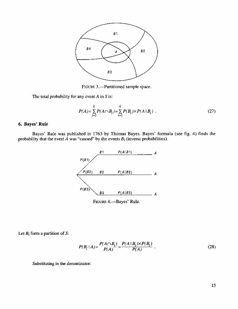
FIGURE3.--Partitionedsamplespace.

Thetotalprobabilityfor anyeventA in S is:

k k

P(A)= Y, P(A_Bi )= Y, P(Bi)×P(A IBi) . (27)i=l i=1

6. Bayes' Rule

Bayes' Rule was published in 1763 by Thomas Bayes. Bayes' formula (see fig. 4) finds the

probability that the event A was "caused" by the events B i (inverse probabilities).

B1 P(AIB1) A

P_ B2 P(AIB2) A

B3 P(AIB3) A

FIGURE 4.--Bayes' Rule.

Let B i form a partition of S:

P(B i IA)=P(AnBi) _ P(A IBi)xP(Bi)

P(A) P(A)(28)

Substituting in the denominator:

15

P(A)=Y.P(A_Bi)=_.,P(A IBi)xP(Bi) , (29)

we obtain Bayes' formula as:

P(AIBi)P(B i)P(B i IA)= k

_, P(A IB i) P(B i )i=l

(30)

The unconditional probabilities P(Bi) are called the "prior" probabilities. The conditional

probabilities P(Bi A) are called the "posterior" probabilities.

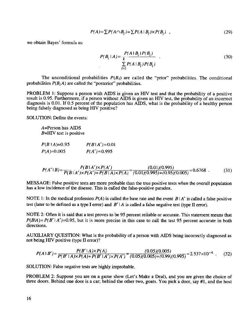
PROBLEM 1: Suppose a person with AIDS is given an HIV test and that the probability of a positiveresult is 0.95. Furthermore, if a person without AIDS is given an HIV test, the probability of an incorrectdiagnosis is 0.01. If 0.5 percent of the population has AIDS, what is the probability of a healthy personbeing falsely diagnosed as being HIV positive?

SOLUTION: Define the events:

A=Person has AIDS

B=HIV test is positive

P(B IA)=0.95

P(A)=0.005

P(BIA')=O.O1

P(A')=0.995

P( A' I P( B IA')xP( A') (0.01)(0.995)B)= P( B IA')xP(A')+ P( B IA)×P( A) = (0.01)(0.995)+(0.95)(0.005) =0.6768 . (31)

MESSAGE: False positive tests are more probable than the mae positive tests when the overall populationhas a low incidence of the disease. This is called the false-positive paradox.

NOTE 1: In the medical profession P(A) is called the base rate and the event B IA' is called a false positive

test (later to be defined as a type I error) and B' IA is called a false negative test (type II error).

NOTE 2: Often it is said that a test proves to be 95 percent reliable or accurate. This statement means that

P(BIA)= P(B'IA')=0.95, but it is more precise in this case to call the test 95 percent accurate in bothdirections.

AUXILIARY QUESTION: What is the probability of a person with AIDS being incorrectly diagnosed asnot being HIV positive (type II error)?

P(B" IA)xP(A) (0.05)(0.005)P(A IB')= P(B" IA)xP(A)+ P(B" IA')xP(A') = (0.05)(0.005)+(0.99)(0.995) =2"537x10-4 " (32)

SOLUTION: False negative tests are highly improbable.

PROBLEM 2: Suppose you are on a game show (Let's Make a Deal), and you are given the choice ofthree doors. Behind one door is a car; behind the other two, goats. You pick a door, say #1, and the host

16

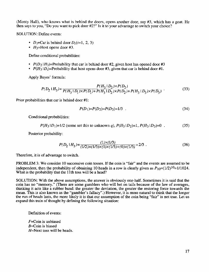
(Monty Hall), who knows what is behind thedoors,opensanotherdoor, say#3, which hasa goat.Hethensaysto you,"Do youwantto pick door#2?" Is it to youradvantageto switchyourchoice?

SOLUTION:Defineevents:

• Di=Car is behind door Di(i=l, 2, 3)

• H3=Host opens door #3.

Define conditional probabilities:

• P(D2 IH3)=Probability that car is behind door #2, given host has opened door #3• P(H3 IDi)--Probability that host opens door #3, given that car is behind door #1.

Apply Bayes' formula:

P(H 3 ID2)×P(D 2)

PfD 2 In3)= P(H3 ID1)×PfD1)+P(H 3 ID2)×P(D2)+PfH 3 ID3)×P(D3) . (33)

Prior probabilities that car is behind door #1:

P(D 1)=P(D2)=P(D3)= 1/3 . (34)

Conditional probabilities:

P(H3 ID1)=l/2 (some set this to unknown q), P(H3 ID2)=l, P(H 3 ID3)=0 . (35)

Posterior probability:

(1)x(1/3) 2/3 (36)P(D2 In3)= (1/2)×(1/3)×(1)×(1/3)+(0)×(1/3) - "

Therefore, it is of advantage to switch.

PROBLEM 3: We consider 10 successive coin tosses. If the coin is "fair" and the events are assumed to be

independent, then the probability of obtaining 10 heads in a row is clearly given as P10=(1/2)10=111024.

What is the probability that the 1 lth toss will be a head?

SOLUTION: With the above assumptions, the answer is obviously one-half. Sometimes it is said that thecoin has no "memory." (There are some gamblers who will bet on tails because of the law of averages,thinking it acts like a rubber band: the greater the deviation, the greater the restoring force towards themean. This is also known as the "gambler's fallacy".) However, it is more natural to think that the longerthe run of heads lasts, the more likely it is that our assumption of the coin being "fair" is not true. Let usexpand this train of thought by defining the following situation:

Definition of events:

F=Coin is unbiased

B=Coin is biased

H=Next toss will be heads.

17

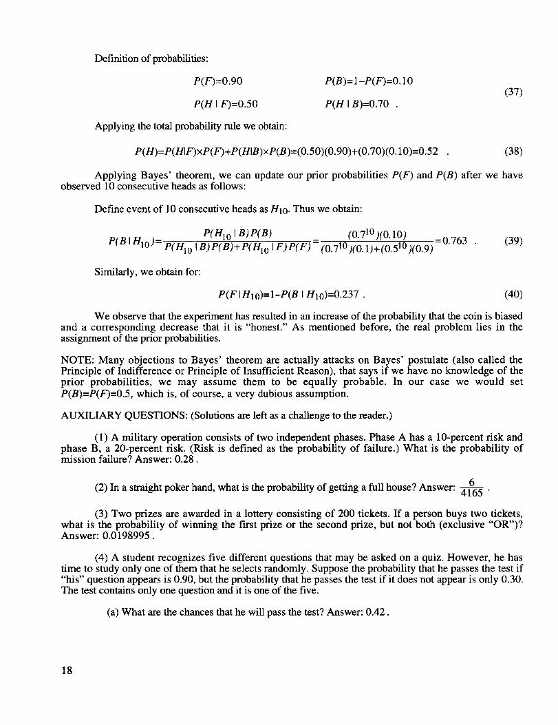
Definitionof probabilities:

P(F)=0.90

P(H I F)=0.50

P(B)=I-P(F)=O.IO

P(H IB)=0.70 .

(37)

Applying the total probability rule we obtain:

P (H)=P( HIF)xP( F)+ P (HIB )xP( B )=( 0.50 )( 0.90 )+( 0. 7 0 )( O. 10)=0.52 (38)

Applying Bayes' theorem, we can update our prior probabilities P(F) and P(B) after we haveobserved 10 consecutive heads as follows:

Define event of 10 consecutive heads as H10. Thus we obtain:

P(HIo IB)P(B) = (0.710)(0. lO) =0.763P(BIHIo)= P(Hlo IB)P(B)+P(Hlo I F)P(F) (0.710)(0.1)+(0.510)(0.9)

(39)

Similarly, we obtain for:

P(F IHlo)= 1-P(B I H10)=0.237 • (40)

We observe that the experiment has resulted in an increase of the probability that the coin is biasedand a corresponding decrease that it is "honest." As mentioned before, the real problem lies in theassignment of the prior probabilities.

NOTE: Many objections to Bayes' theorem are actually attacks on Bayes' postulate (also called thePrinciple of Indifference or Principle of Insufficient Reason), that says if we have no knowledge of theprior probabilities, we may assume them to be equally probable. In our case we would set

P(B)=P(F)=0.5, which is, of course, a very dubious assumption.

AUXILIARY QUESTIONS: (Solutions are left as a challenge to the reader.)

(1) A military operation consists of two independent phases. Phase A has a 10-percent risk andphase B, a 20-percent risk. (Risk is defined as the probability of failure.) What is the probability ofmission failure? Answer: 0.28.

(2) In a straight poker hand, what is the probability of getting a full house? Answer: 64165 "

(3) Two prizes are awarded in a lottery consisting of 200 tickets. If a person buys two tickets,what is the probability of winning the first prize or the second prize, but not both (exclusive "OR")?Answer: 0.0198995.

(4) A student recognizes five different questions that may be asked on a quiz. However, he hastime to study only one of them that he selects randomly. Suppose the probability that he passes the test if"his" question appears is 0.90, but the probability that he passes the test if it does not appear is only 0.30.The test contains only one question and it is one of the five.

(a) What are the chances that he will pass the test? Answer: 0.42.

18

(b) If thestudentpassedthetest,what is theprobability that"his" questionwasaskedon thetest?Answer:0.4286.

(5) A manhastwo pennies--one"honest" andone two-headed.A pennyis chosenat random,tossed,andobservedto comeupheads.Whatis theprobabilitythattheothersideis alsoahead?Answer:2/3.

D. Probability Distributions

In order to define probability distributions precisely, we must first introduce the followingauxiliary concepts.

1. Set Function

We are all familiar with the concept of a function from elementary algebra. However, a precisedefinition of a function is seldom given. Within the framework of set theory, however, it is possible tointroduce a generalization of the concept of a function and identify some rather broad classification offunctions.

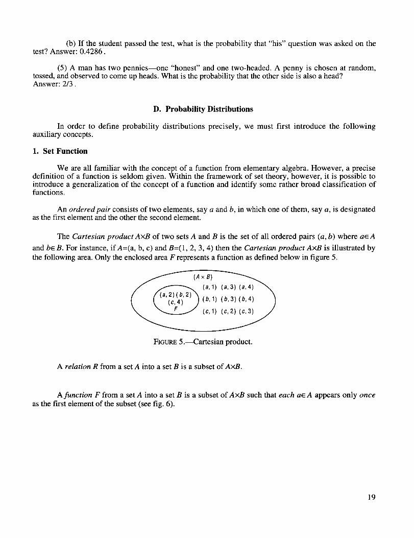
An ordered pair consists of two elements, say a and b, in which one of them, say a, is designatedas the f'u'st element and the other the second element.

The Cartesian product AxB of two sets A and B is the set of all ordered pairs (a, b) where a_ A

and be B. For instance, if A=(a, b, c) and B=(1, 2, 3, 4) then the Cartesian product AxB is illustrated by

the following area. Only the enclosed area F represents a function as defined below in figure 5.

(Ax B) (a, 3) (a,4__(a, 1)

(b, 1) (b,3)(b, 4) )/

(c, 1) (c, 2)(__

FIGtmE 5.---Cartesian product.

A relation R from a set A into a set B is a subset of AxB.

A function F from a set A into a set B is a subset of AxB such that each a_ A appears only once

as the flu'st element of the subset (see fig. 6).

19

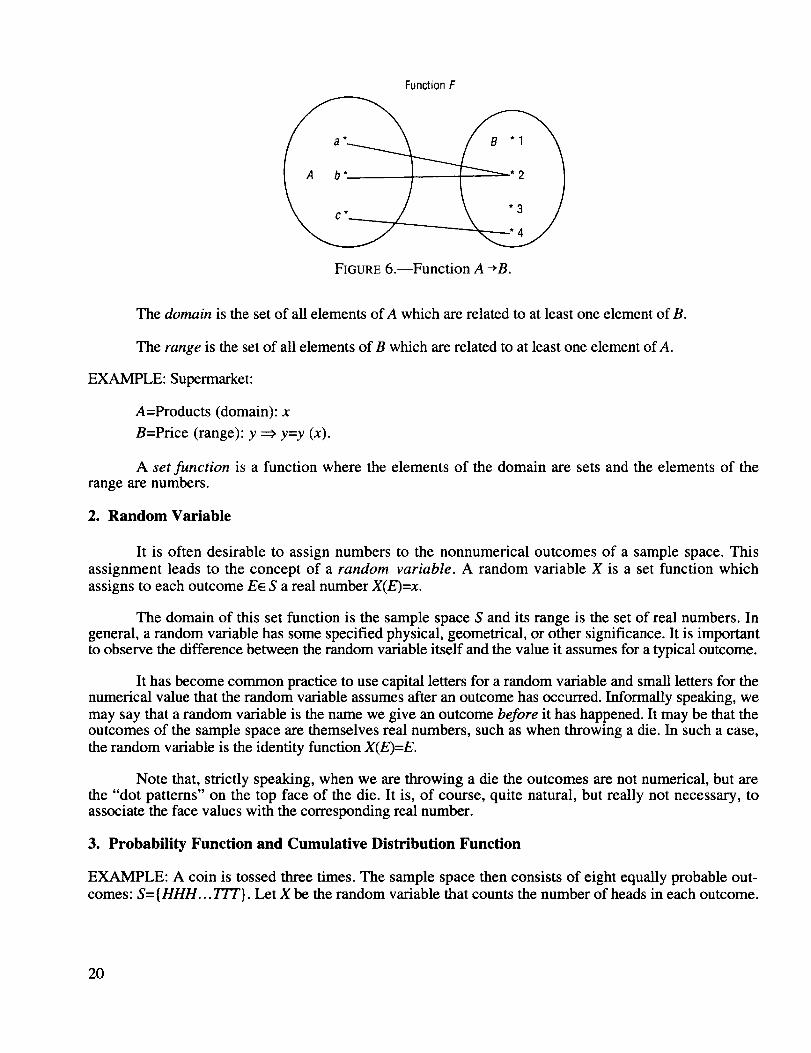
FunctionF

FIGURE 6.--Function A-*B.

The domain is the set of all elements of A which are related to at least one element of B.

The range is the set of all elements of B which are related to at least one element of A.

EXAMPLE: Supermarket:

A=Products (domain): x

B=Price (range): y _ y=y (x).

A set function is a function where the elements of the domain are sets and the elements of therange are numbers.

2. Random Variable

It is often desirable to assign numbers to the nonnumerical outcomes of a sample space. This

assignment leads to the concept of a random variable. A random variable X is a set function which

assigns to each outcome E_ S a real number X(E)=x.

The domain of this set function is the sample space S and its range is the set of real numbers. Ingeneral, a random variable has some specified physical, geometrical, or other significance. It is importantto observe the difference between the random variable itself and the value it assumes for a typical outcome.

It has become common practice to use capital letters for a random variable and small letters for thenumerical value that the random variable assumes after an outcome has occurred. Informally speaking, we

may say that a random variable is the name we give an outcome before it has happened. It may be that theoutcomes of the sample space are themselves real numbers, such as when throwing a die. In such a case,

the random variable is the identity function X(E)=E.

Note that, strictly speaking, when we are throwing a die the outcomes are not numerical, but arethe "dot patterns" on the top face of the die. It is, of course, quite natural, but really not necessary, toassociate the face values with the corresponding real number.

3. Probability Function and Cumulative Distribution Function

EXAMPLE: A coin is tossed three times. The sample space then consists of eight equally probable out-comes: S= {HHH... TTT}. Let X be the random variable that counts the number of heads in each outcome.

20

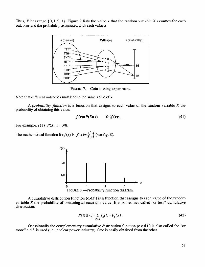
Thus,X has range {0, 1, 2, 3}. Figure 7 lists the value x that the random variable X assumes for each

outcome and the probability associated with each value x.

S (Domain) R(Range)

H'I-I'* I _'--_"- * I"-'_--_

HTH* _ kj.----* "a----.J

"<22/ v

P (Probability)

318

,1/8

FIGURE 7.--Coin-tossing experiment.

Note that different outcomes may lead to the same value of x.

A probability function is a function that assigns to each value of the random variable X theprobability of obtaining this value:

f(x)=P(X=x) 0<f(x)<l . (41)

For example, f(1 )=P(X= 1)=3/8.

The mathematical function forf(x)is f(x)=l(3x)(see fig. 8).

f(x)

3/8

1/8

o 1 2 3FIGURE 8.--Probability function diagram.

v X

A cumulative distribution function (c.d.f.) is a function that assigns to each value of the random

variable X the probability of obtaining at most this value. It is sometimes called "or less" cumulativedistribution:

oP(X < x) = t<xf x (t) = Fx (x)(42)

Occasionally the complementary cumulative distribution function (c.c.d.f.) is also called the "ormore" c.d.f, is used (i.e., nuclear power industry). One is easily obtained from the other.

21

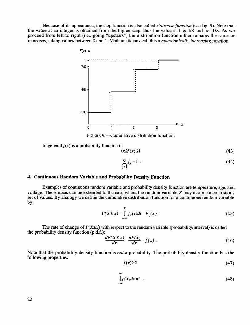
Becauseof its appearance,thestepfunctionis alsocalledstaircase function (see fig. 9). Note thatthe value at an integer is obtained from the higher step, thus the value at 1 is 4/8 and not 1/8. As weproceed from left to right (i.e., going "upstairs") the distribution function either remains the same or

increases, taking values between 0 and 1. Mathematicians call this a monotonically increasing function.

F(x)

1

7/8

4/8

1/8

ii

'k|

0 1 2 3I= X

FIGURE 9.---Cumulative distribution function.

In generalf(x) is a probability function if:

O_<f(x)__l (43)

E,fx =1 . (44){x}

4. Continuous Random Variable and Probability Density Function

Examples of continuous random variable and probability density function are temperature, age, and

voltage. These ideas can be extended to the case where the random variable X may assume a continuousset of values. By analogy we define the cumulative distribution function for a continuous random variableby:

X

P(X<x)= _ fx(t)dt=Fx(x ) (45)--oo

The rate of change of P(X<x) with respect to the random variable (probability/interval) is calledthe probability density function (p.d.f.):

dP(X<x) dE(x) _. ,-_ = -_ = y(x) . (46)

Note that the probability density function is not a probability. The probability density function has thefollowing properties:

f(x)>O (47)

to

_f(x)dx=l . (48)--to

22

Also notethattheprobabilityof anull event(impossibleevent)iszero.Theconverseis notneces-sarily true for a continuousrandomvariable,i.e., if X is a continuous random variable, then an eventhaving probability zero can be a possible event. For example, the probability of the possible event that aperson is exactly 30 years old is zero.

Alternate definitions:

P(x<X<x+dx)=f(x) dx (49)

b

P(a < X <b)= Sf (x)dx = F(b)-F(a) .a

(5O)

E. Distribution (Population) Parameters

One of the purposes of statistics is to express the relevant information contained in the mass of databy means of a relatively few salient features that characterize the distribution of a random variable. Thesenumbers are called distribution or population parameters. We generally distinguish between a knownparameter and an estimate thereof, based on experimental data, by placing a hat symbol (A) above the

estimate. We usually designate the population parameters by Greek letters. Thus, fi denotes an estimate of

the population parameter/l. In the following, the definitions of the population parameters will be given

for continuous distributions. The definitions for the discrete distribution are obtained by simply replacingintegration by appropriate summation.

1. Measures of Central Tendency (Location Parameter)

a. Arithmetic Mean (Mean, Average, Expectation, Expected Value). The mean is the mostoften used measure of central tendency. It is defined as:

OO

# = Sxf(x)dx (51)--oo

The definition of the mean is mathematically analogous to the definition of the center of mass in dynamics.That is the reason the mean is sometimes referred to as the first moment of a distribution.

b. Median (Introduced in 1883 by Francis Galton). The median m is the value that dividesthe total distribution into two equal halves, i.e.,

m

F(m)= _f(x)dx=ll2 (52)--00

c. Mode (Thucydides, 400 B.C., Athenian Historian). This is also called the most probablevalue, from the French "mode," meaning "fashion." It is given by the maximum of the distribution,i.e., the value of x for which:

df(x) =0 (53)dx

23

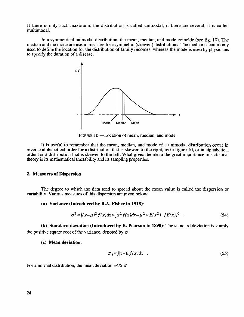
If there is only such maximum, the distribution is called unimodal; if there are several, it is calledmultimodal.

In a symmetrical unimodal distribution, the mean, median, and mode coincide (see fig. 10). Themedian and the mode are useful measure for asymmetric (skewed) distributions. The median is commonlyused to define the location for the distribution of family incomes, whereas the mode is used by physiciansto specify the duration of a disease.

r(x)[

Mode Median Mean

•_ x

FIGURE 10.--Location of mean, median, and mode.

It is useful to remember that the mean, median, and mode of a unimodal distribution occur in

reverse alphabetical order for a distribution that is skewed to the right, as in figure 10, or in alphabeticalorder for a distribution that is skewed to the left. What gives the mean the great importance in statisticaltheory is its mathematical tractability and its sampling properties.

2. Measures of Dispersion

The degree to which the data tend to spread about the mean value is called the dispersion orvariability. Various measures of this dispersion are given below:

(a) Variance (Introduced by R.A. Fisher in 1918):

tr 2 = S(x-I.t) 2 f(x)dx = Sx 2 f(x)d.x-l.t 2 = E(x 2 )-{E(x)} 2

(h)

the positive square root of the variance, denoted by tr.

(54)

Standard deviation (Introduced by K. Pearson in 18911): The standard deviation is simply

(c) Mean deviation:

Crd = Slx- _lf (x )dx

For a normal distribution, the mean deviation --4/5 tr.

(55)

24

(d)

mean ]2 as:

Coefficient of variation (c.o.v.): The c.o.v, gives the standard deviation relative to the

c.o.v.=0-/]2 (56)

It is a nondimensional number and is often expressed as a percentage. Note that it is independent of theunits used.

3. Quantiles

The quantile of order p is the value _p such that P(X<__p)=p.

For p=0.5 Median

p=0.25 Quartile

p=0.10 Decile

p=0.01 Percentile.

The jth quantile is obtained by solving for x:

X

fin= Sf(x)dx-- t_o

Quantiles are sometimes used as measures of dispersion:

(a) Interquartile range

(b) Semi-interquartile range

(c) Interdecile range

Q=_0.75-_0.25

Q2=0.5 x (_0.75-_0.25)

a10=_0.90--_0.10

For a normal distribution, the semi-interquartile range =2/3 0-.

(57)

4. Higher Moments

Other important population parameters referred to as "higher moments" are given below:

(a) Skewness:

a 3 = ]23/0- 3, where//3 = S(x _]2)3 f(x)dx (58)

A distribution has a positive skewness (is positively skewed) if its long tail is on the right and a negativeskewness (is negatively skewed) if its long tail is on the left.

(b) Kurtosis:

O_4 = ]24/0"4, where ]24 = _(X--]2 )4 f(x)dx (59)

25

Kurtosismeasuresthe degreeof "peakedness"of a distribution,usually in comparisonwith a normaldistribution,which hasthekurtosisvalueof 3.

(c) Momentsof kth order:

Moments about the origin (raw moments):

#'_ = E(x k) = _xk f (x)dx . (60)

Moments about the mean (central moments):

Pk = E(x-lt) k = _(x-p)k f(x)dx . (61 )

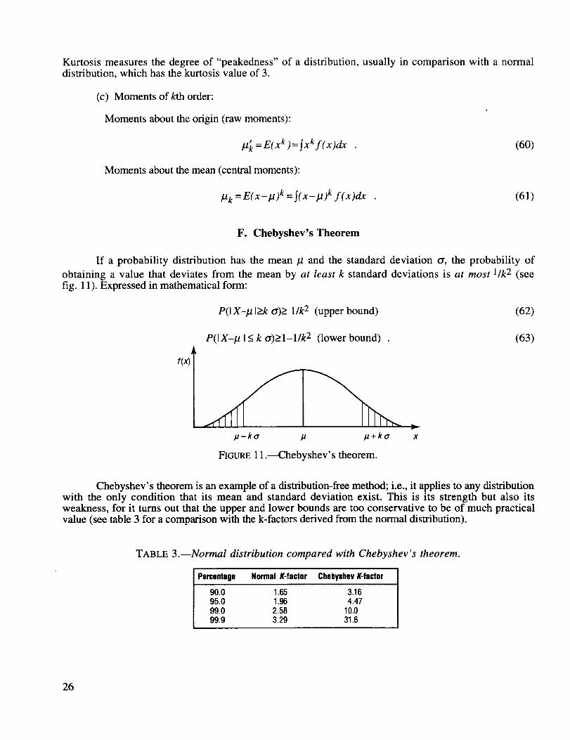
F. Chebyshev's Theorem

If a probability distribution has the mean/z and the standard deviation or, the probability of

obtaining a value that deviates from the mean by at least k standard deviations is at most 1/k2 (see

fig. 11). Expressed in mathematical form:

P(I X-# I>k or)> 1/k 2 (upper bound) (62)

P(I X-# I< k o')>l-1/k 2 (lower bound) .

.u _+ko" x

(63)

FIGURE 11.--Chebyshev' s theorem.

Chebyshev's theorem is an example of a distribution-free method; i.e., it applies to any distributionwith the only condition that its mean and standard deviation exist. This is its strength but also itsweakness, for it turns out that the upper and lower bounds are too conservative to be of much practicalvalue (see table 3 for a comparison with the k-factors derived from the normal distribution).

TABLE 3.--Normal distribution compared with Chebyshev's theorem.

Percentage Normal A-factor Chebyshev E-factor

90.0 1.65 3.1695.0 1.96 4.4799.0 2.58 10.099.9 3.29 31.6

26

The so-called Camp-Meidel correction for symmetrical distributions is only a slight improvement. It

replaces the upper bound by 1/(2.25xk2).

G. Special Discrete Probability Functions

1. Binomial Distribution

Assumptions (Bernoulli trials) of binomial distribution are:

• There are only two possible outcomes for each trial ("success" and "failure")

• The probability p of a success is constant for each trial.

• There are n independent trials.

The random variable X denotes the number of successes in n trials. The probability function is thengiven by:

f(x)= P(X= x)=(n)px(1-p) n-x for x=O,1...n

Mean la=np

Variance _2=npq where q=l-p

Skewness a3=q__p_/npq

1-6pq

Kurtosis _4 = 3+

(Note that any of the subsequent BASIC programs can be readily edited to run on any computer.)

(64)

Binomial probabilities can be calculated using the following BASIC program, which is based onthe recursion formula:

10:15:20:25:30:35:40:45:50:55:

f(x)=p× n-x x f(x-1) (65)q x

"CUMBINOMIAL"

CLEAR:INPUT "N="; N, "P="; P,"X="; X

Q=I-P:F=Q^N:B=F:S=0IF X=0 GOTO 55FOR I= I TO X

E=P*(N-I+I)/Q/IF=F*E:S=S+FNEXT ICF=S+BPRINT CF:PRINT F

27

EXAMPLE: N=6, P=0.30, x=3

CF=0.9295299996, F=1.852199999E-01.

Simulation of Bernoulli trials can be performed using the following BASIC program:

100: "BINOMIAL"

105: INPUT "N=";N, "P=";P

110: S=0115: FOR I=1 TO N120: U=RND .5125: IF U<P LET X=I GOTO 135130: X=0135: S=S+X140: NEXT I

145: PRINT S: GOTO 110

2. Poisson Distribution

The Poisson distribution is expressed as:

fix)= #Xx_-/_ for x=-0, 1,2, 3 ...oo (66)

Mean: #=b/

Variance: o'2=-#

The Poisson distribution is a limiting form of the binomial distribution when n--,oo, p--*0, and

rip=# remain constant. The Poisson distribution provides a good approximation to the binomial

distribution when n>20 and p<0.05.

The Poisson distribution has many applications that have no direct connection with the binomialdistribution. It is sometimes called the distribution of rare events; i.e., "number of yearly dog bites in NewYork City." It might be of historical interest to know that its first application by Ladislaus von Bortldewicz

(Das Gesetz der Kleinen Zahlen, Teubner, Leipzig, 1898) concerned the number of Prussian cavalrymenkilled by horse kicks.

The following BASIC program is based on the recursion formula:

10:15:20:

f(x)=_f(x-1) (67)

"POISSON"

INPUT "M=";M, "X=";XP=EXP-M:S= 1 :Q= 1

28

25: IF X=0 LET F=P GOTO 5030: FOR I=1 TO X

35: Q=Q*M/I: S=S+Q40: NEXT I

45: F=P*S:P=P*Q50: PRINT F:PRINT P60: END

EXAMPLE: /_=2.4 x=4

F=9.041314097×10 -1 , P=f(x)=1.2540848986×10 -1

3. Hypergeometric Distribution

This distribution is used to solve problems of sampling inspection without replacement, but it hasmany other applications (i.e., Florida State Lottery, quality control, etc.).

Its probability function is given by:

for x=0, 1, 2, 3...n (68)

where N=lot size, n=sample size, a=number of defects in lot, and x=number of defects (successes)in sample.

Mean: l.t=n×-_ Variance: cr2-nxax(N-a)x(N-n)- N 2 ×(N-l)

(69)

The following BASIC program calculates the hypergeometric probability function and itsassociated cumulative distribution by calculating the logarithms (to avoid possible overflow) of the threebinomial coefficients of the distribution and subsequent multiplcation and division, which appears in line350 as summation and difference of the logarithms.

300:305:310:

"HYPERGEOMETRIC"

INPUT "N=";N, "N1, "A=";AINPUT "X=";X 1

315:320:

NC=N:KC=N1 :GOSUB 400CD=C

325:330:335:340:345:350:355:360:

CH=0: FOR X=0 TO X1NC=A:KC=X:GOSUB 400CI=CNC=N-A:KC=N1-X:GOSUB 400

C2=C

HX-EXP (CI+C2-CD)CH=CH+HXNEXT X:BEEP3

29

365:370:

PRINT CH: PRINT HXEND

400:405:410:415:420:

C=0:;M=NC-KCIF KC=0RETURNFORI=1TO KCC=C+LN((M+I)/I)NEXT I : RETURN

4. Negative Binomial (Pascal) Distribution

The negative binomial, or Pascal, distribution finds application in tests that are terminated after a

predetermined number of successes has occurred. Therefore, it is also called the binomial waiting time

distribution. Its application always requires a sequential-type situation. The random variable X in this case

is the number of trials necessary for k successes to occur. (The last trial is always a success!)

The probability function is readily derived by observing that we have a binomial distribution up tothe last trial, which is then followed by a success. As in the binomial distribution, the probabilityp of a success is again assumed to be constant for each trial.

Therefore:

for .70.where x=Number of trials

k=-Number of successes

p=Probability of success.

Also:

Mean: bt= k Variance: 0 -2 - k(1-p)p p2 (71)

The special case k=l gives the geometric distribution. The geometric distribution finds application inreliability analysis, for instance, if we investigate the performance of a switch that is repeatedly turned onand off, or a mattress to withstand repeated pounding in a "torture test."

PROBLEM: What is the probability of a mattress surviving 500 thumps if the probability of failure as the

result of one thump is p=l/200?

SOLUTION: The probability of surviving 500 thumps is P(X>500) and is called the reliability of themattress. The reliability function R(x) is related to the cumulative distribution as:

R(x)=l-F(x) . (72)

Since the geometric probability function is given asf(x)=p(1-p)x-l, we obtain for the reliability ofthe mattress:

30

R(x) = Y_f(x) = (1- p)500 = (0.995) 500 = 0.0816 (73)x=501

It is sometimes said that the geometric distribution has no "memory" because of the relation:

P(X>xo+x IX>xo)=P(X>x) . (74)

In other words, the reliability of a product having a geometric (failure) distribution is independent of its

past history, i.e., the product does not age or wear out. These failures are called random failures.

Sometimes the transformation z=x-k is made where z is the number of failures. Then the

probability function is given by:

( )pkxqzforz=O,1,2,3... (75)f(z) = k+z-1

and these are the successive terms in pk(1-q)-Z, a binomial expression with a negative index.

When a program of the binomial distribution is available, the negative probabilities can be obtainedby the simple identity:

fp(X Ik, p)=k fb(klx ' p) (76)

where the subscript p denotes the Pascal distribution and the subscript b the binomial distribution.

PROBLEM: Given a 70-percent probability that a job applicant is made an offer, what is the probability of

needing exactly 12 sequential interviews to obtain eight new employees?

SOLUTION: x=12, k=8, p=0.7 (/.t=l 1.42, o'----2.2) (77)

18, 0.7=(11)(0.7) 8 (0.3)4=0.1541 (78)fg(12

A more interesting complementary relationship exists between the cumulative Pascal and the

cumulative binomial distribution. This is obtained as follows: The event that more than x sequential trials

are required to have k successes is identical to the event that x trials resulted in less than k successes.Expressed in mathematical terms we have:

Pp(X>x Ek,p)=Pb( K<k l x, p) . (79)

The cumulative Pascal distribution can then be obtained from the cumulative binomial by the

relationship:

Fp(xlk, p)=l-Fb(k-1 Ix, p) . (80)

PROBLEM: Given a 70-percent probability that a job applicant is made an offer, what is the probability

that, at most, 15 sequential interviews are required to obtain eight new employees?

SOLUTION: Fp(1518, 0.7)=I-Fb(7 115, 0.7)=0.95=95 percent . (81)

31

H. Special Continuous Distributions

1. Normal Distribution

The normal distribution is the most important continuous distribution for the following reasons:

• Many random variables that appear in connection with practical experiments and observations arenormally distributed. This is a consequence of the so-called Central Limit Theorem or NormalConvergence Theorem to be discussed later.

• Other variables are approximately normally distributed.• Sometimes a variable is not normally distributed, but can be transformed into a normally

distributed variable.

• Certain, more complicated distributions can be approximated by the normal distribution.

The normal distribution was discovered by De Moivre (1733). It was known to Laplace no laterthan 1774, but is usually attributed to Carl F. Gauss. He published it in 1809 in connection with the theoryof errors of physical measurements. In France it is sometimes called the Laplace distribution.Mathematicians believe the normal distribution to be a physical law, while physicists believe it to be amathematical law.

The normal distribution is defined by the equation:

_,(x-,321 2\y 1 2\ tr J

g(y)=---_e- ,O<y<oo . f(x)- e for-_<x<_ (82)

Mean: p=p

Skewness:a3=0

Variance: 0"2=¢r2

Kurtosis: tr.4=3.

The cumulative distribution function of this density function is an integral that cannot be evaluatedby elementary methods.

The existing tables are given for the so-called standard normal distribution by introducing the

standardized random variable. This is obtained by the following transformation:

(X--lg)

z =----_-- (83)

In educational testing, it is known as the standard score or the "z-score." It used to be called"normal deviate" until someone perceived that this is a contradiction in terms (oxymoron), in view of thefact that deviates are abnormal.

Every random variable can be standardized by the above transformation. The standardized random

variable always has the mean p=0 and the standard deviation o'=-1.

The cumulative distribution of every symmetrical distribution satisfies the identity:

F(-x)=l-F(x) . (84)

32

Theerror function is defined as:

X

_(x)=_ Ie -t2 at (85)*"_ 0

It is related to the normal cumulative distribution by:

(86)

where

X

F(x)= 1 Se_U2/2 du (87)

We are often interested in the probability of a normal random variable to fall below (above) or

between k standard deviations from the mean. The corresponding limits are called one-sided or two-sided

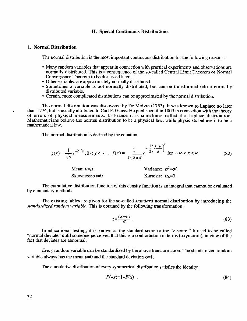
tolerance limits. Figures 12 and 13 are given as illustrations.

Two-Sided Limits

Pr (I_-Ka<X<I_+K_)=A

+2

FIGURE 12.--Normal distribution areas: two-sided tolerance limits.

Stated, there is a 95.46-percent probability that a normal random variable will fall between

the +_2 cr limits.

33

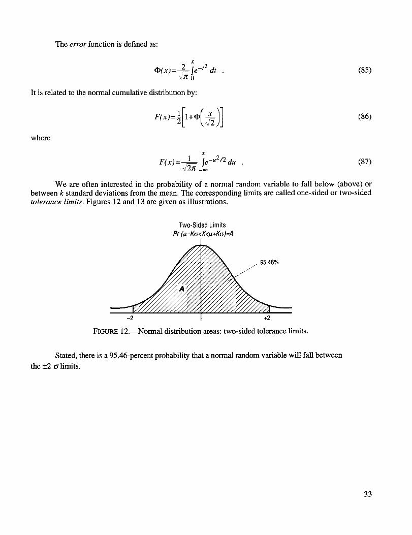
One-SidedLimits

Pr(X</_ + K(_)= F

FIGURE 13.--Normal distribution areas: one-sided tolerance limits.

Stated, there is a 97.73-percent probability that a normal random variable will fall below (above)

the +2o" (-2o') limit.

The relationship between the two areas A and F is:

A=2F- 1 or F=(A + 1)/2 .

A normal random variable is sometimes denoted as:

X=N(#, tr2)=Gauss (/.t, o"a) .

(88)

(89)

The standard normal variable or standard score is thus:

Z=N(0, 1)=Gauss (0, 1) (90)

Table 4 gives the normal scores ("K-factors") associated with different levels of probability.

TABLE 4.--Normal K-factors.

One-Sided Two-Sided

Percent K1 Percent 1(299.90 3.0902 99.90 3.290599.87 3.0000 99.73 3.000099.00 2.3263 99.00 2.575897.73 2.0000 95.46 2.000095.00 1.6448 95.00 1.960090.00 1.2815 90.00 1.644985.00 1.0364 85.00 1.439584.13 1.0000 80.00 1.281680.00 0.8416 75.00 1.150375.00 0.6744 70.00 1.036470.00 0.5244 68.27 1.000065.00 0.3853 65.00 0.934660.00 0.2533 60.00 0.841655.00 0.1257 55.00 0.755450.00 0.0000 50.00 0.6745

34

As was already mentioned, the normal p.d.f, cannot be integrated in closed form to obtain thec.d.f.. One could, of course, use numerical integration, such as Simpson's Rule or the Gaussianquadrature method, but it is more expedient to calculate the c.d.f, by using power series expansions,continued fraction expansions, or some rational (Chebyshev) approximation. An excellent source of

reference is Handbook of Mathematical Functions by Milton Abramowitz and Irene A. Stegun (eds.).

The following approximation for the cumulative normal distribution is due to C. Hastings, Jr.:

_x2/2 5

F(x)=l e Y, anyn (91)_/2n" n=l

1y = 0 < x < to (92)

1 + 0.2316419x

where

a1=0.3193815

a2=-0.3565638

a3=1.781478a4=-1.821256

a5=1.330274.

E_or=<7E-7

EXAMPLE: x=2.0 F(x)=0.97725

Sometimes it is required to work with the so-called inverse normal distribution, where the area F is

given and the associated K-factor (normal score) has to be determined. A useful rational approximation for

this case is given by equation (93) (equation 26.2.23 in the Handbook of Mathematical Functions) asfollows:

Then

We define Q(kp)=p where Q=I-F and 0 <p<0.5 .

c o + clt + c2 t2

Kp = t - 1 + dlt + d2 t2 + d3 t3 4-e (p), t = _/S2 gnp (93)

and le(p)l<4.5xl0 -4,

where

c0=2.515517

c1=0.802853

c3=0.010328

d1=1.432788

d2=0.189269

d3=0.001308.

A more accurate algorithm is given by the following BASIC program. It calculates the inverse

normal distribution based on the continued fraction formulas also found in the Handbook of

Mathematical Functions. Equation (94) in this reference (equation 26.2.14 in the Handbook) is used for

x >2, equation (95) for x<2 (equation 26.2.15 in the Handbook, and the Newton-Raphson method using

initial values obtained from equation (98).

35

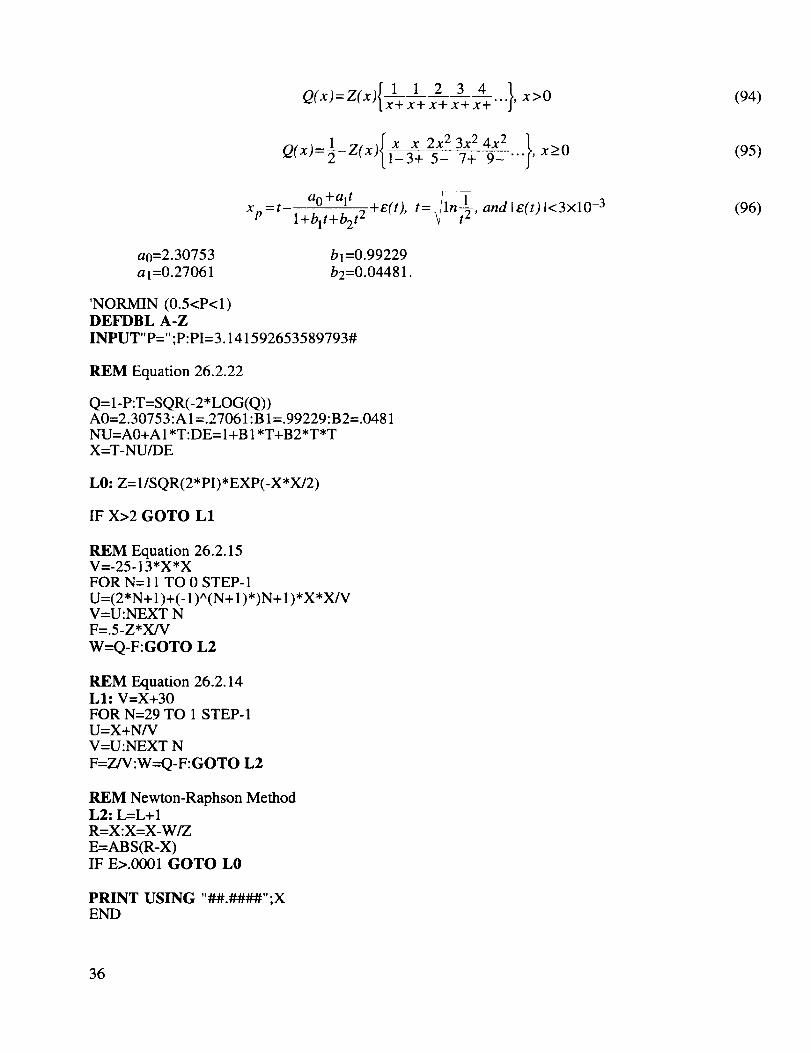
Q x =z x {11234 }x>0X+ XA- X+ "'" '

7+9_

a0=2.30753

a1=0.27061

'NORMIN (0.5<P<l)DEFDBL A-Z

ao+alt _-e(t), t= lln- _,andle(t)l<3xlO -3Xp = t- l+blt+b2t2

b1=0.99229

b2=0.04481.

INPUT"P=";P:PI=3.141592653589793#

REM Equation 26.2.22

Q=I-P:T=SQR(-2*LOG(Q))A0=2.30753 :A 1=.27061 :B 1=.99229:B2=.0481NU=A0+A 1*T:DE= I+B 1*T+B2*T*TX=T-NU/DE

L0: Z= 1/SQR(2*PI)*EXP(-X*X/2)

IF X>2 GOTO L1

REM Equation 26.2.15V=-25-13*X*XFOR N= 11 TO 0 STEP-1

U=(2*N+I)+(-1)^(N+I)*)N+I)*X*X/VV=U:NEXT NF=.5-Z*X/V

W=Q-F:GOTO L2

REM Equation 26.2.14LI" V=X+30FOR N=29 TO 1 STEP-1U=X+N/VV=U:NEXT N

F=Z/V:W=Q-F:GOTO L2

REM Newton-Raphson MethodL2" L=L+IR=X:X=X-W/Z

E=ABS(R-X)IF E>.0001 GOTO L0

PRINT USING "##.####";XEND

(94)

(95)

(96)

36

The normal distribution is often used for random variables that assume only positive values such asage, height, etc. This can be done as long as the probability of the random variable being smaller thanzero, i.e., P(X<0), is negligible. This is the case when the coefficient of variation is less than 0.3.

The normal and other continuous distributions are often used for discrete random variables. This is

admissible if their numerical values are large enough that the associated histogram can be reasonably

approximated by a continuous probability density function. Sometimes a so-called continuity correctionis suggested which entails subtracting one-half from the lower limit of the cumulative distribution and

adding one-half to its upper limit.

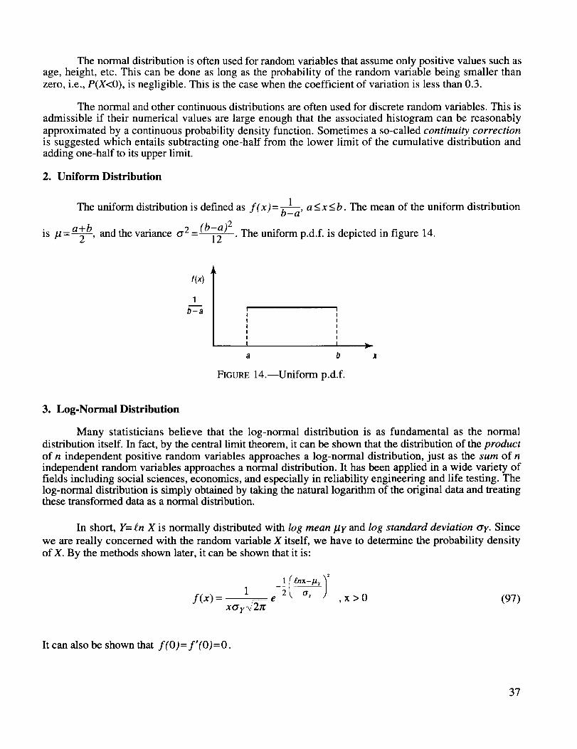
2. Uniform Distribution

The uniform distribution is defined as f(x)= b-Ld, a < x < b. The mean of the uniform distribution

is /.t= a_b and the variance ty 2 (b-a)2' - 12 . The uniform p.d.f, is depicted in figure 14.

f(x)

1

b-a

b

FIGURE 14.--Uniform p.d.f.

3. Log-Normal Distribution

Many statisticians believe that the log-normal distribution is as fundamental as the normal

distribution itself. In fact, by the central limit theorem, it can be shown that the distribution of the product

of n independent positive random variables approaches a log-normal distribution, just as the sum of nindependent random variables approaches a normal distribution. It has been applied in a wide variety offields including social sciences, economics, and especially in reliability engineering and life testing. Thelog-normal distribution is simply obtained by taking the natural logarithm of the original data and treatingthese transformed data as a normal distribution.

In short, Y= £n X is normally distributed with log mean fly and log standard deviation tyy. Since

we are really concerned with the random variable X itself, we have to determine the probability density

of X. By the methods shown later, it can be shown that it is:

1 I _nx-/.t,/21 -2L a, j

f(x) = xcrr_2/_ _ e , x > 0 (97)

It can also be shown that f(O)=f'(O)=O.

37

The mode of the distribution occurs at:

XMode =e _Y-a2

and the median at:

The mean is:

The variance is:

(98)

XMedian = e lar (99)

lax = e I_Y+(1/'2)cr2Y (100)

O'x2= (e2/ar+a2)(err2 -1) . (101)

The distribution has many different shapes for different parameters. It is positively skewed, the

degree of skewness increasing with increasing try.

Some authors define the log-normal distribution in terms of the Briggsian (Henry Briggs, 1556-1630) or common logarithm rather than on the Naperian (John Napier, 1550-1616) or natural logarithm.

The log mean/.ty and the log standard deviation O'y are nondimensional pure numbers.

4. Beta Distribution

This distribution is a useful model for random variables that are limited to a finite interval. It is

frequently used in Bayesian analysis and finds application in determining distribution-free tolerance limits.

The beta distribution is usually defined over the interval (0, 1) but can be readily generalized to

cover an arbitrary interval (x0, Xl). This leads to the probability density function:

1 F(ot+fl)(X-Xo)(a-1)(X-Xo)(fl-1)f(x)= (x 1_Xo) r(a)F(fl) x1-x o 1 Xl -Xo (102)

The standard form of the beta distribution can be obtained by transforming to a beta randomvariable over the interval (0, 1) using the standardized z-value:

x-x 0z = , where 0<_.z__.l (103)

xl-x o

The beta distribution has found wide application in engineering and risk analysis because of its

diverse range of possible shapes (see fig. 15 for different values of a and ft.) The mean and variance ofthe standardized beta distribution is:

_ t_ _2 = O_fl/_ - _--flfl and (104)(ot + fl)E (ot + fl+ l)

38

4.5

4.0

_. 3.5"" 3.0

_. 2.5N 2.o

1,5tL

1.0

0,5

00

_=8

a=2_'_a=5

0.2 0.4 0.6 0.8X

a=l,6=1

FIGURE 15.--Examples of standardized beta distribution.

The cumulative beta distribution is known as the incomplete beta function. An interesting anduseful relationship exists between the binomial and beta distribution. If X is a binomial random variable

with parameters p and n, then:

1-p

F(n+l) _tn-x-l(1-t) x dtP(X<x)= F(n-_)F(x+l) 0

(105)

5. Gamma Distribution

The gamma distribution is another two-parameter distribution that is suitable for fitting a widevariety of statistical data. It has the following probability density function:

XCt-1 e-X/#f(x)- for x>O and a, fl>O . (106)

r(a)fl a

A typical graph of the gamma p.d.f, is shown in figure 16.

f(x)

FIGURE 16.---Gamma distribution.

39

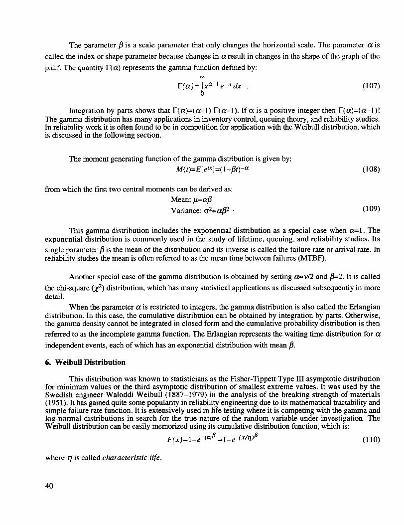
The parameterfl is a scale parameter that only changes the horizontal scale. The parameter a is

called the index or shape parameter because changes in a result in changes in the shape of the graph of the

p.d.f. The quantity F(a) represents the gamma function defined by:oo

F(a)= Sx ct-l e -x dx (107)0

Integration by parts shows that F(a)=(a-1) F(a-1). If a is a positive integer then F(a)=(a-1)!

The gamma distribution has many applications in inventory control, queuing theory, and reliability studies.In reliability work it is often found to be in competition for application with the Weibull distribution, whichis discussed in the following section.

The moment generating function of the gamma distribution is given by:

M ( t)=E[ etX]=(1-flt) -a (108)

from which the first two central moments can be derived as:

Mean: It=aft

Variance: o2=af12 • (109)

This gamma distribution includes the exponential distribution as a special case when a=l. The

exponential distribution is commonly used in the study of lifetime, queuing, and reliability studies. Its

single parameter fl is the mean of the distribution and its inverse is called the failure rate or arrival rate. In

reliability studies the mean is often referred to as the mean time between failures (MTBF).

Another special case of the gamma distribution is obtained by setting a=vl2 and fl=2. It is called

the chi-square (2"2) distribution, which has many statistical applications as discussed subsequently in moredetail.

When the parameter a is restricted to integers, the gamma distribution is also called the Erlangiandistribution. In this case, the cumulative distribution can be obtained by integration by parts. Otherwise,the gamma density cannot be integrated in closed form and the cumulative probability distribution is then

referred to as the incomplete gamma function. The Erlangian represents the waiting time distribution for tx

independent events, each of which has an exponential distribution with mean ft.

6. Weibull Distribution

This distribution was known to statisticians as the Fisher-Tippett Type Ill asymptotic distributionfor minimum values or the third asymptotic distribution of smallest extreme values. It was used by theSwedish engineer Waloddi Weibull (1887-1979) in the analysis of the breaking strength of materials(1951). It has gained quite some popularity in reliability engineering due to its mathematical tractability andsimple failure rate function. It is extensively used in life testing where it is competing with the gamma andlog-normal distributions in search for the true nature of the random variable under investigation. TheWeibull distribution can be easily memorized using its cumulative distribution function, which is:

F (x ) = 1-e -ax# = 1-e-(X/O )# (110)

where r/is called characteristic life.

40

It is easily seen that for x=-r/the cumulative distribution is always 1-1/e=0.6321 regardless of the

value of the parameter 13. The first form of the cumulative distribution is somewhat easier to manipulate

mathematically. If the parameter o_ is known, the characteristic life can be calculated as r/=a -l/ft. The

probability density is obtained by simple differentiation of the cumulative distribution.

There are two special cases that give rise to distributions of particular importance:

CASE 1: r= 1

This is the exponential distribution, which is also a special case of the gamma distribution. It has manyimportant applications in reliability and life testing.

CASE 2:fl=2

This is the Raleigh distribution. It describes the distribution of the magnitude of winds if the north-southwinds and the east-west winds are independent and have identical normal distributions with zero mean. Itis also the distribution for the circular error probability (CEP). Another application arises in randomvibration analysis where it can be shown that the envelope of a narrow-band random process has aRayleigh distribution.

7. Extreme Value (Gumbel) Distribution

This distribution is seldom used in reliability engineering and in life and failure data analysis. It is,however, used for some types of "largest observations" such as flood heights, extreme wind velocities,

runway roughness, etc. It is more precisely called the largest extreme value distribution. Sometimes it isalso called the Gumbel distribution, after Emil J. Gumbel (1891-1967), who pioneered its use. It is brieflypresented here for the sake of completeness.

Its cumulative distribution function is:

F(x)=exp {- exp (-(x-_,)lb') } , --_ < X < to (111)

Mean: p=A+y_, where )=0.57722 (Euler's constant)

Variance: cr2=Tr252/6 .

(112)

(113)

I. Joint Distribution Functions

1. Introduction

In many engineering problems we simultaneously observe more than one random variable. For

instance, in the cantilever beam shown in figure 17, we encounter five random variables: the length L, the

force P, the Young's modulus E, the deflection t_, and the moment of inertia I z. In general, all of them

will, of course, have different distributions as indicated in figure 17.

41

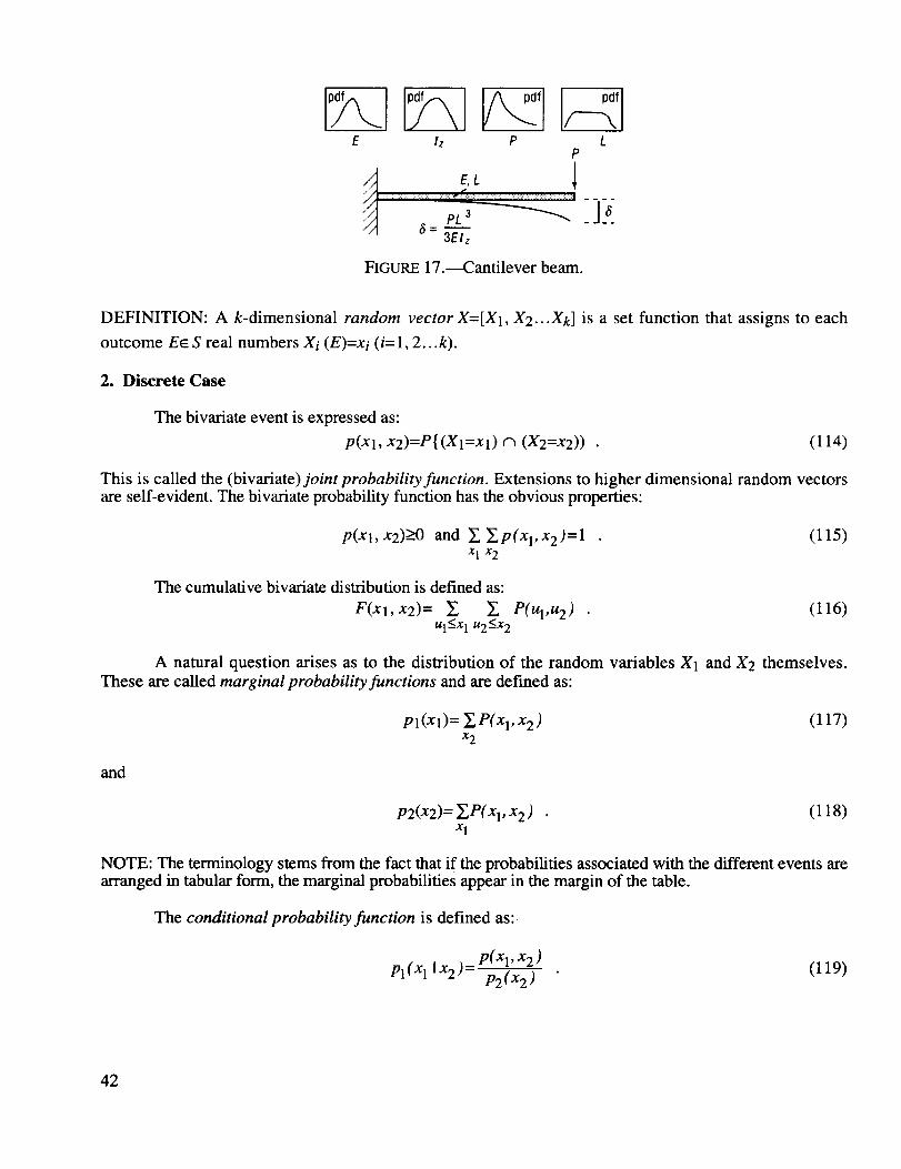
E lz P LP

FIGURE 17.---Cantilever beam.

DEFINITION: A k-dimensional random vector X=[X1, X2...X/_] is a set function that assigns to each

outcome Ee S real numbers Xi (E)=xi (i=1,2...k).

2. Discrete Case

The bivariate event is expressed as:

p(xl, x2)=P{(Xl=Xl) n (X2=x2)) • (114)

This is called the (bivariate) joint probability function. Extensions to higher dimensional random vectorsare self-evident. The bivariate probability function has the obvious properties:

p(xl, x2)>0 and _ Y_P(Xl,X2)=l (115)x1 x2

The cumulative bivariate distribution is defined as:

F(xt,x2)= E Eu1<x 1 u2<x 2

P(Ul,U2 ) (116)

A natural question arises as to the distribution of the random variables X1 and X2 themselves.

These are called marginal probability functions and are defined as:

pl (Xl)= Y P(x 1, x 2 ) (117)x 2

and

p2(x2)= Y?(x 1, x 2 ) (118)x 1

NOTE: The terminology stems from the fact that if the probabilities associated with the different events arearranged in tabular form, the marginal probabilities appear in the margin of the table.

The conditional probability function is defined as:

p( x 1, x 2 )

Pl (Xl Ix 2 ) = P2 (x2)(119)

42

3. Continuous Case

The extension to continuous random variable is easily achieved by replacing summation byintegration (and usually by replacing p with f).

DEFINITION: The c.d.f, is defined as:

x I x2

F(Xl,X2)=P(X1 <Xl, X2 <x2)= S Sf(ul,U2)dUl du2 (120)--oo --_

and the bivariate probability density is obtained by partial differentiation as:

3 2 F(x 1, x 2 )

f (x 1,x 2 ) = tgXloax2(121)

Similarly, the conditional probability density is defined as:

f (Xl,X 2)

f(x I IX 2) = f2 (X2)(122)

4. Independent Random Variables and Bayes' Rule

The notion of independence, which was introduced in connection with intersections of events, canbe analogously defined for random vectors. Informally speaking, when the outcome of one randomvariable does not affect the outcome of the other, we state that the random variables are independent.

DEFINITION: Iff(xl, x2) is the joint probability density of the random variables XI and X2, theserandom variables are independent if and only if:

f(Xl, X2)=fl (Xl) f2(x2) (123)

Extensions to the multivariate case are obvious.

Sometimes the concept of independence is defined in terms of the cumulative distributions. In thiscase we have:

F(xl, x2)=F1 (Xl) F2(x2) (124)

Bayes' Rule. In recent years there has been a growing interest in statistical inference, which looksupon parameters (mean, standard deviations, etc.) as random variables. This approach is known asBayesian estimation. It provides a formal mechanism for incorporating our degree of personal judgmentabout an unknown parameter into the estimation theory before experimental data are available. As thesedata become available, the personal judgment is constantly updated to reflect the increase in knowledgeabout a certain situation.

DEFINITION 1: The probability distribution ho(p) of the parameter p, which expresses our belief

about the possible value p before a sample is observed, is called the prior distribution ofp. We reiterate

that ho(p) makes use of the additional subjective information about the value p prior to taking a sample.

43

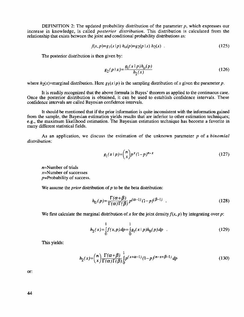
DEFINITION 2: The updatedprobability distribution of the parameterp, which expresses our

increase in knowledge, is called posterior distribution. This distribution is calculated from therelationship that exists between the joint and conditional probability distributions as:

f(x, p)=gl (x Ip) ho(P)=g2(P Ix) h2(x) . (125)

The posterior distribution is then given by:

g2(P tx)= gl (x Ip)ho(P) (126)hz(x)

where h2(x)=marginal distribution. Here g l (xlp) is the sampling distribution of x given the parameter p.

It is readily recognized that the above formula is Bayes' theorem as applied to the continuous case.Once the posterior distribution is obtained, it can be used to establish confidence intervals. Theseconfidence intervals are called Bayesian confidence intervals.

It should be mentioned that if the prior information is quite inconsistent with the information gainedfrom the sample, the Bayesian estimation yields results that are inferior to other estimation techniques;e.g., the maximum likelihood estimation. The Bayesian estimation technique has become a favorite inmany different statistical fields.

As an application, we discuss the estimation of the unknown parameter p of a binomialdistribution:

gl(X l p)=(nx)pX (1-p)n-x (127)

n=Number of trials

x=Number of successes

p=Probability of success.

We assume the prior distribution ofp to be the beta distribution:

['(Ot+fl) n(a-1) (l_p)([3-1)hO (P)= r(a)r(fl) _

(128)

We first calculate the marginal distribution of x for the joint densityf(x, p) by integrating over p:

1 1

h2(x)= If(x,p) dp= Igl(x Ip)ho(P)dP0 0

(129)

This yields:

h2(x)=(n) F(°t+fl ) 1[.p(X+a-1) (l_p)(n-x+fl-1) dpx r(a)r(fl)o

(130)

or:

44

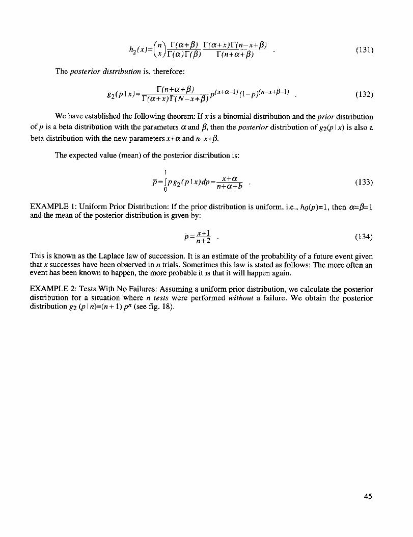
h2(x)=(nxl (131)

The posterior distribution is, therefore:

g2(P Ix)= F(n+ct+fl) .n(x+a-1)F(a+x) F(N-x+fl) r (l-P) (n-x+[3-1) (132)

We have established the following theorem: If x is a binomial distribution and the prior distribution

ofp is a beta distribution with the parameters t_ and fl, then the posterior distribution of g2(P Ix) is also a

beta distribution with the new parameters x+tx and n-x+fl.

The expected value (mean) of the posterior distribution is:

1

p=ipg2(ptx)dp = x+ao n+a+b

(133)

EXAMPLE 1" Uniform Prior Distribution: If the prior distribution is uniform, i.e., h0(p)=l, then a=fl=land the mean of the posterior distribution is given by:

x+l (134)P=n+2

This is known as the Laplace law of succession. It is an estimate of the probability of a future event giventhat x successes have been observed in n trials. Sometimes this law is stated as follows: The more often an

event has been known to happen, the more probable it is that it will happen again.

EXAMPLE 2: Tests With No Failures: Assuming a uniform prior distribution, we calculate the posterior

distribution for a situation where n tests were performed without a failure. We obtain the posteriordistribution g2 (P In)=(n + 1) pn (see fig. 18).

45

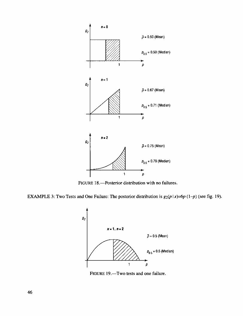
n=Og2

1

,5= 0.50 (Mean)

Po.5= 0.50 (Median)

Ii,

P

g2

n=l

,5= 0.67 (Mean)Po.5= 0.71 (Median)

1 p

g2n=2

,5= 0.75 (Mean)

Po.5= 0.79 (Median)

1 p

FIGURE 18.--Posterior distribution with no failures.

EXAMPLE 3: Two Tests and One Failure: The posterior distribution is g2(plx)=6p (l-p) (see fig. 19).

g2

x=l,n=2

,5= 0.5 (Mean)

Po.5= 0.5 (Median)

T--

P

FIGURE 19.--Two tests and one failure.

46

EXAMPLE 4: Bayesian Confidence Limits: In reliability studies we are usually interested in one-sided

confidence limits for the reliability p of a system. Given the posterior distribution g2(P Ix) for the reliability

p, we obtain the lower Bayesian (l--a) confidence limit as:

1

Jg2(plx)dp=l-a

p,(135)

The lower confidence limit is obtained by solving this equation for the lower integration limit PL(see fig. 20).

g2 (plx)

PLr

p

FIGURE 20.--Lower confidence limit.

The upper Bayesian (1 -a) confidence limit is similarly obtained from the equation:

Pu

Sg2(plx)dp=l-a (136)0

If there are no test failures the posterior distribution is:

g2(P Ix)-(n+l) pn (137)

Inserting this posterior distribution into the above equation for the lower confidence limit for the

reliability (probability of success), we can solve it for the (l-a) lower confidence limit in closed form andobtain:

(n+l) =a (138)5

This lower confidence limit is often referred to as the demonstrated reliability when it is applied to a

system which has undergone n tests without a failure.

It is sometimes necessary to find the number of tests required to demonstrate a desired reliability

for a (1 - _x) confidence level. This can be easily obtained by solving the above equation for n, which inthis case is:

47

_na1 (139)

n= gn p L

For instance, if it is required to demonstrate a 99-percent reliability at the 50-percent confidence level, it isnecessary to run 68 tests without a failure.

If no confidence level is specified, the 50-percent confidence level is generally assumed. This isespecially the case for high reliability systems.

The non-Bayesian confidence limit for the binomial parameter p for the above case is given by:

PL n =a (140)

It is somewhat more conservative than the Bayesian limit because it requires one more test to demonstrate

the same level of reliability.

J. Mathematical Expectation

In many problems of statistics, we are interested not only in the expected value of a random

variable X, but in the expected value of a function Y=g(X).

DEFINITION: Let X=(XI, X2...Xn) be a continuous random vector having a joint probability density

f(x)=f(xl, x2...Xn) and let u(X) be a function of X. The mathematical expectation is then defined as:

oo

E[u(X)] = _u(x)f(x) dx . (141)

For a discrete random vector the integral is replaced by a corresponding summation. Sometimes

E[.] is called the "'expected value operator."

The vector notation introduced here simplifies the expression for the multiple integral appearing inthe definition of the mathematical expectation. A further consideration of this general case is beyond thescope of the present text.

EXAMPLE: Chuck-A-Luck: The concept of a mathematical expectation arose in connection with the gamesof chance. It serves as an estimate of the average gain (or loss) one will have in a long series of trials. In

this context the mathematical expectation is also called the expected profit. It is defined by the sum of allthe products of the possible gains (losses) and the probabilities that these gains (losses) will occur.Expressed mathematically, it is given as:

E = _,a ipi (142)

It is important to keep in mind that the coefficients ai in the above equation are positive when they

represent gains and negative when they represent losses.

In betting odds, the expected profit is set equal to zero (E=0). For example, if the odds of favoringan event are 3:1, the probability of the event happening is 3/4 and the expected profit is:

E=$1 (3/4)-$3 (1/4)=0 . (143)

48

In Scarne's New Complete Guide to Gambling, John Scarne puts it this way: "When you make abet at less than the correct odds, which you always do in any organized gambling operation, you arepaying the operator the percentage charge for the privilege of making a bet. Your chances of winning haswhat is called a 'minus expectation.' When you use a system you make a series of bets, each with a minusexpectation. There is no way of adding minuses to get a plus."

As an illustration for calculating the expected profit, we take the game of Chuck-A-Luck. In thisgame the player bets on the toss of three dice. He is paid whatever he bets for each die that shows hisnumber.

The probability of any number showing on a die is p=l/6. Let the probability of one number

showing on three dice be Pl, of two numbers P2, and of three numbers P3. Then:

pl=3 pq2=3 (1/6) (5/6) (5/6)=75/216 (144)

p2=3p2q=3 (1/6) (1/6) (5/6)=15/216 (145)

p3=p3=(1/6) (1/6) (1/6)=1/216 . (146)

The expected profit is, therefore:

E=($1) p1+($2) p2+($3) p3-($1) PLOSS (147)

where

PLOS S= 1-(p 1+p2+P3)= 125/216 (148)

E=lX75+2×15+3×l . 125 17 .-, (149)Thus, 216 1x2--i-6=-2--_/_

or: E=-7.87 cents/dollar. (150)

The house percentage is, therefore, 7.87 percent.

As may be noticed, we have already encountered a few special cases of mathematical expectation,such as the mean, variance, and higher moments of a random variable. Beyond these, the following simplefunctions are of particular interest.

1. Covariance

The covariance measures the degree of association between two random variables X1 and X2. It isdefined as follows:

Cov (X1, X2)=_12=E[(XI-II 1) (X2-//2)]

Performing the multiplication we obtain an alternate form of the covariance as:

Cov (Xl, X2)=E[X1 × X2]-E[X1 ] E[X2]=E[X1 x X2]-_ 1/-12

(151)

(152)

49

The covariancecanbemadenondimensionalby dividing by the standarddeviationof the tworandomvariables.Thus,weget theso-calledcorrelation coefficient:

/C°v(XI'X2) °'12 (153)P= ,,,v(x1) ,-\,,,'v(x2) o'lo'2

It can be shown that if X1 and X2 are independent, then p=0. This is true for both discrete and

continuous random variables. The converse of this statement is not necessarily true, i.e., we can have p=0

without the random variables being independent. In this case the random variables are called uncorrelated.

It can also be shown that the value ofp will be on the interval (-1, +1), that is:

-l<p <+1 (154)

2. Linear Combinations

The linear combination of the elements of a random vector X_=(X1, X2...Xn) is defined as

u(_X)=Y=ao+al X+... +an Xn (155)

The mean and variance of this linear combination is:

n n

E( Y )= l-ty = ao +i_=lai E( Xi )=ao +i_ailti , (156)

and:

n n n

V(Y)=o'2=i_=la2o'2 +i--_1 _"aiajo'iJj=li_j

(157)

If the variables are independent, the expression for the variance of Y is simplified because the covariance

terms o-ij are zero. In this case the variance reduces to:

n

o-2 = i=]=la2o-2 (158)

Notice that all these relationships are independent of the distribution of the random variablesinvolved.

K. Functions of Random Variables

In many engineering applications we meet with situations in which we have to determine theprobability density of a function of random variables. This is especially true in the theory of statisticalinference, because all quantities used to estimate population parameters or to make decisions about apopulation are functions of the random observation appearing in a sample.

50

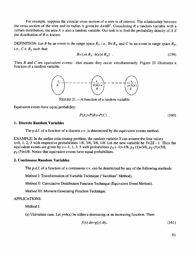
For example,supposethecircularcrosssectionof a wire is of interest.Therelationshipbetweenthecrosssectionof thewire andits radiusis givenby A=zcR 2. Considering R a random variable with a

certain distribution, the area A is also a random variable. Our task is to find the probability density of A ifthe distribution of R is known.

DEFINITION: Let B be an event in the range space Rx, i.e., Be Rx, and C be an event in range space Ry,

i.e., C _ Ry such that:

B= {xe Rx : h(x)_ Ry } (159)

Then B and C are equivalent events--that means they occur simultaneously. Figure 21 illustrates afunction of a random variable.

FIGURE 21.--A function of a random variable.

Equivalent events have equal probability:

P(A )=P(B)=P( C) (160)

1. Discrete Random Variables

The p.d.f, of a function of a discrete r.v. is determined by the equivalent events method.

EXAMPLE: In the earlier coin-tossing problem, the random variable X can assume the four values

x=0, 1, 2, 3 with respective probabilities 1/8, 3/8, 3/8, 1/8. Let the new variable be Y=2X- 1. Then the

equivalent events are given by y=-l, 1, 3, 5 with probabilities py (-1)=1/8, py (1)=3/8, py (3)=3/8,

py (5)= 1/8. Notice that equivalent events have equal probabilities.

2. Continuous Random Variables

The p.d.f, of a function of a continuous r.v. can be determined by any of the following methods:

Method I: Transformation of Variable Technique ("Jacobian" Method).

Method II: Cumulative Distribution Function Technique (Equivalent Event Method).

Method Ilk Moment Generating Function Technique.

APPLICATIONS:

Method I:

(a) Univariate case. Let y=h(x) be either a decreasing or an increasing function. Then:

f(x) dx=g(y) dy, (161)

51

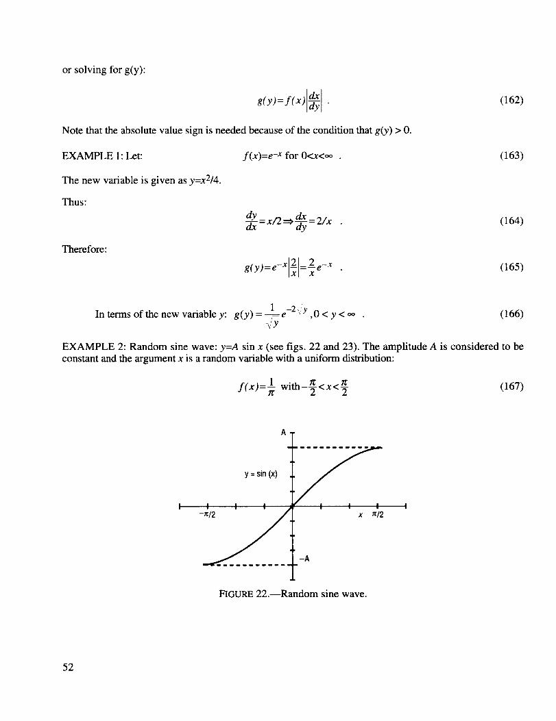
or solvingfor g(y):

g(y)=f(x) _yy .

Note that the absolute value sign is needed because of the condition that g(y) > 0.

f(x)=e -x for 0<x<o_EXAMPLE 1: Let:

The new variable is given as y=x2/4.

Thus:

Therefore:

d_ = x/2=::, _-_-_=2/x

-x 2 2 -xg(y)=e x =x e

(162)

(163)

(164)

(165)

1 -2 _yIn terms of the new variable y: g(y)=--_e ,0<y<oo

3/Y(166)

EXAMPLE 2: Random sine wave: y=A sin x (see figs. 22 and 23). The amplitude A is considered to be

constant and the argument x is a random variable with a uniform distribution:

f(x)= 1 with-_<x<_ (167)

y = sin(x)

-_ _/2

FIGURE 22.--Random sine wave.

52

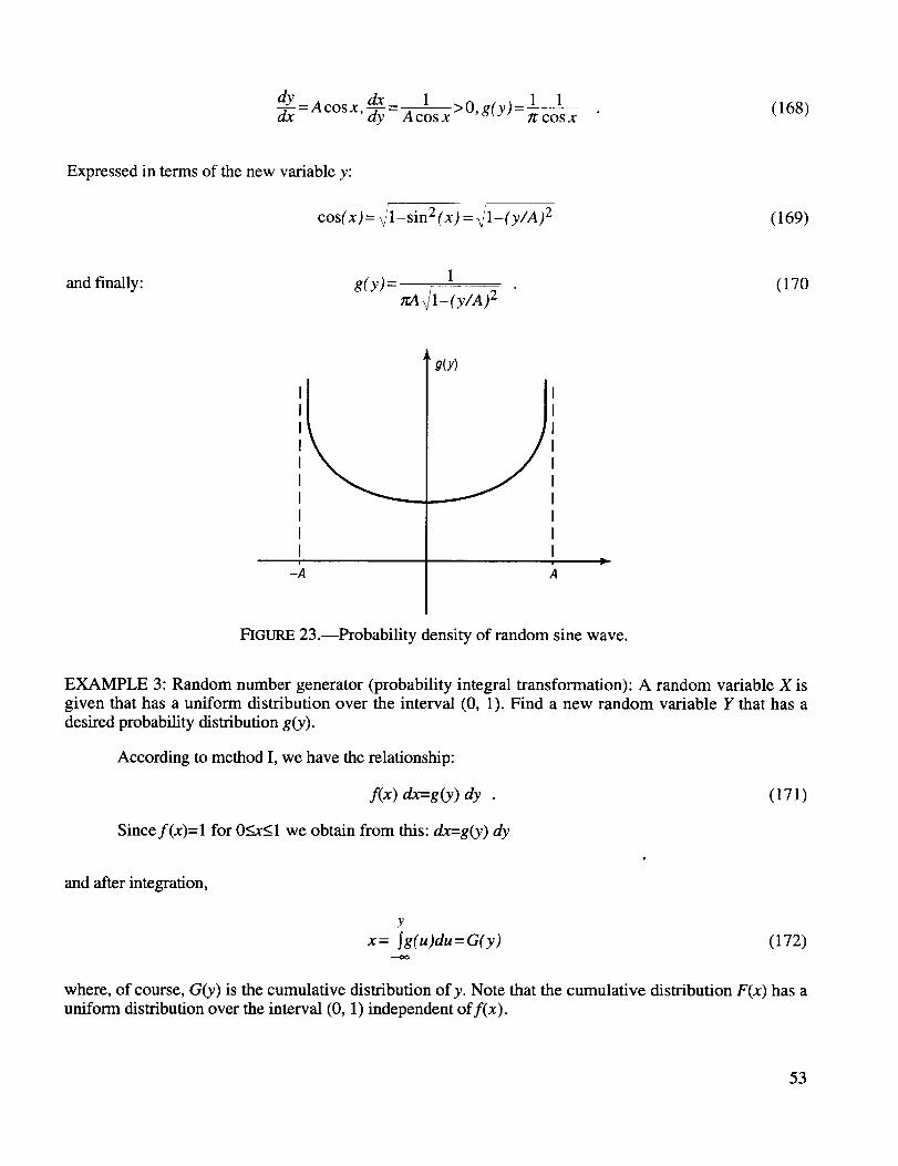
dx _ 1 (168)=Ac°SX' dy Ac sx >O'g(y)= l 1If COS X

Expressed in terms of the new variable y:

cos(x) = \el-sin 2 (x ) = \�1-(y/A) 2 (169)

and finally: g(y)_ -- 1 __ . (170rtA _' l-( y/A )2

-A

g(Y)

11,,

A

FIGURE 23.--Probability density of random sine wave.

EXAMPLE 3: Random number generator (probability integral transformation): A random variable X is

given that has a uniform distribution over the interval (0, 1). Find a new random variable Y that has a

desired probability distribution g(y).

According to method I, we have the relationship:

f(x) dx=-g(y)dy . (171)

Sincef(x)=l for 0_.x<l we obtain from this: dx=g(y) dy

and after integration,

Y

x = _g(u)du = G(y) (172)

where, of course, G(y) is the cumulative distribution of y. Note that the cumulative distribution F(x) has a

uniform distribution over the interval (0, 1) independent off(x).

53

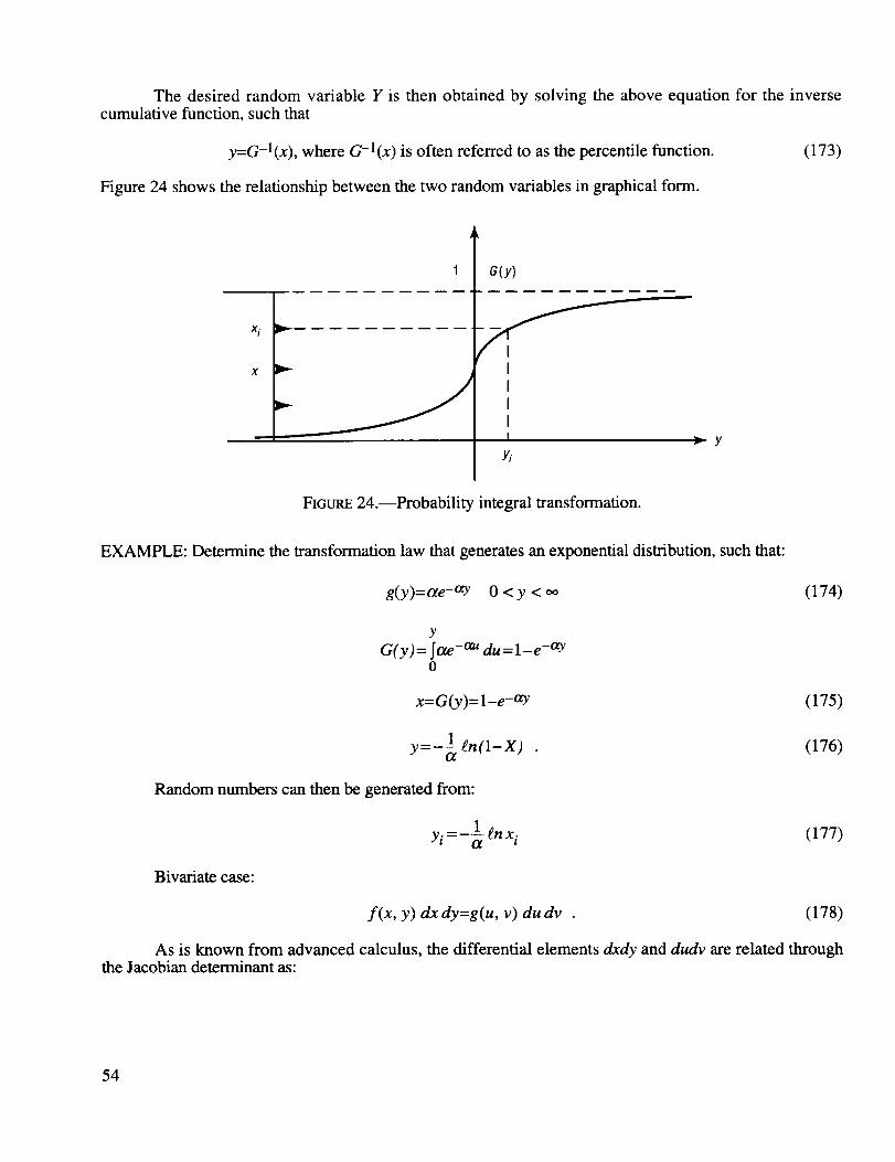
The desiredrandomvariable Y is then obtained by solving the above equation for the inversecumulative function, such that

y=G -l(x), where G-l(x) is often referred to as the percentile function. (173)

Figure 24 shows the relationship between the two random variables in graphical form.

1 I G(y)

Xi m

Ix

y

FIGURE 24.--Probability integral transformation.

EXAMPLE: Determine the transformation law that generates an exponential distribution, such that:

g(y)=ae-aY 0 < y < oo (174)

y

G( y )= Str.e-au du =l-e -ay0

x=G(y)= l-e-aY (175)

Y=-I gn (l-X) (176)

Random numbers can then be generated from:

_ 1Yi - --ff gn x i (177)

Bivariate case:

f(x, y) dx dy=g(u, v) du dv . (178)

As is known from advanced calculus, the differential elements dxdy and dudv are related throughthe Jacobian determinant as:

54

dxdy= dudv=J(u, v)dudv where J(u,v)=Jacobian determinant. (179)

The new joint probability density function is, then:

g(u, v)=f(x, y) IJ(u, v) l . (180)

EXAMPLE 1: If the random variables X1 and X2 have a standard normal distribution N(0, 1), the ratioXI[X 2 has a Cauchy distribution.

Let Yl =Xl[X2 and y2=x2 _ xl=Yl/Y2 and x2=y 2.

The partial derivatives are:

3x]_ 3x1_ 3x2_ &2_

_11 -y2, _22 -yl, _1 -0, _22 -1 (181)

and the Jacobian is then J=Y2.

The joint probability density function is:

. 1x2 _!e_ly2(l+y2e-2X2 Y2 ) Y2g(yl,Y2)=___e-_ 1 ] 2 - 2zr (182)

The marginal distribution is:

g(Yl )= I 1-Le-ly2(I+y2) Y2 dy= I l e-2Y2(I+yl ) d (183)-_ 2zr 0 7r

1

which gives: g(Yl ) =/r(1 + Y)i") (184)

EXAMPLE 2: Box-Muller method: An important use of the Jacobian method for finding the jointprobability density of a function of two or more functions of a random vector is the Box-Muller algorithm.Since its introduction in 1958, it has become one of the most popular method for generating normalrandom variables. It results in high accuracy and compares favorably in speed with other methods. Themethod actually generates a pair of standard normal variables from a pair of uniform random variables.

Consider the two independent standard normal random variables x and y with densities:

1 lx2 1 ly2

f(x) = _ e-_ and f(y) = _ e-2(185)

55

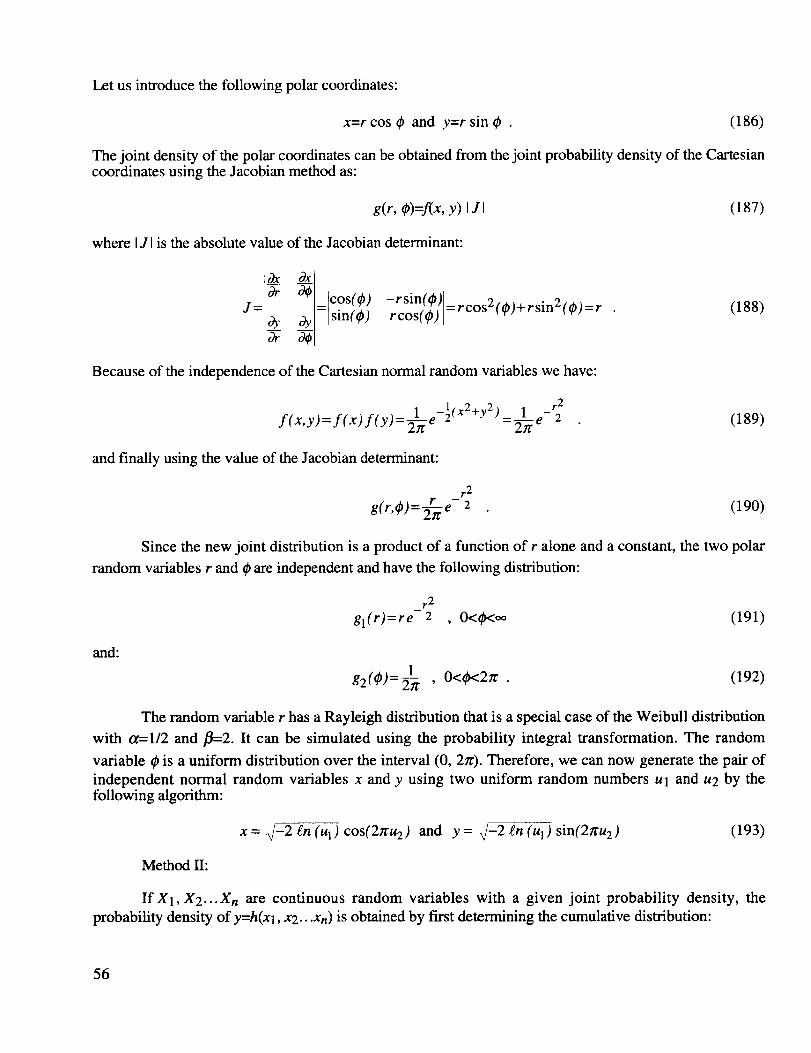
Let us introducethefollowingpolarcoordinates:

x=r cos _ and y=r sin ¢ . (186)

The joint density of the polar coordinates can be obtained from the joint probability density of the Cartesiancoordinates using the Jacobian method as:

g(r, ¢)=f(x, y) IJI (187)

where IJ I is the absolute value of the Jacobian determinant:

_ _ cos(_) -rsin(d?)J= Or _- sin(_) rcos((p) =rc°s2(O)+rsin2((9)=r (188)

Because of the independence of the Cartesian normal random variables we have:

r 2r.. 1 e-l(x2+v 2),_ 1

f(x,y)=f(x)]{y)=_ " = -2--_e 2 (189)

and finally using the value of the Jacobian determinant:

r 2

g(r, dp)=_e 2 (190)

Since the new joint distribution is a product of a function of r alone and a constant, the two polar

random variables r and ¢ are independent and have the following distribution:

and:

r 2

gl(r)=re 2 , 0<¢<oo (191)

g2(¢)=_-_-_ , O<tir<2zr . (192)

The random variable r has a Rayleigh distribution that is a special case of the Weibull distribution

with a=l/2 and fl=2. It can be simulated using the probability integral transformation. The random

variable ¢ is a uniform distribution over the interval (0, 2n:). Therefore, we can now generate the pair of

independent normal random variables x and y using two uniform random numbers Ul and u2 by thefollowing algorithm:

Method II:

x = _/-2 £n (u 1) cos(2zru 2) and y = _/-2 £n (u 1) sin(2_u 2) (193)

If X1, X2...Xn are continuous random variables with a given joint probability density, the

probability density of y=h(xl, x2...Xn) is obtained by first determining the cumulative distribution:

56

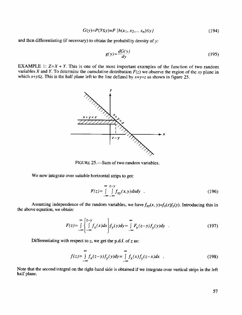
G(y)=P(Y<y)=P [h(xl, x2 .... Xn)<-yl

and then differentiating (if necessary) to obtain the probability density of y:

EXAMPLE

(194)

dG(y) (195)g(Y)= dy

1" Z=X + Y. This is one of the most important examples of the function of two random

variables X and Y. To determine the cumulative distribution F(z) we observe the region of the xy plane in

which x+y<-z. This is the half plane left to the line defined by x+y=z as shown in figure 25.

y

x__._.//////////._.÷

x

FIGURE 25 .--Sum of two random variables.

We now integrate over suitable horizontal strips to get:

Z-y

F(z)= [ [ fxy(X,y)dxdy (196)--o0 --0o

Assuming independence of the random variables, we havefxy(X, y)=fx(X)fy(y). Introducing this inthe above equation, we obtain:

F(z)= L l L f x(x )dxlfy(y)dy= L Fx(z- y) fy(y)dy (197)

Differentiating with respect to z, we get the p.d.f, of z as:

f(z)= [. fx(Z-y)fy(y)dy= [ fx(X)fy(Z-x)dx (198)

Note that the second integral on the right-hand side is obtained if we integrate over vertical strips in the lefthalf plane.

57

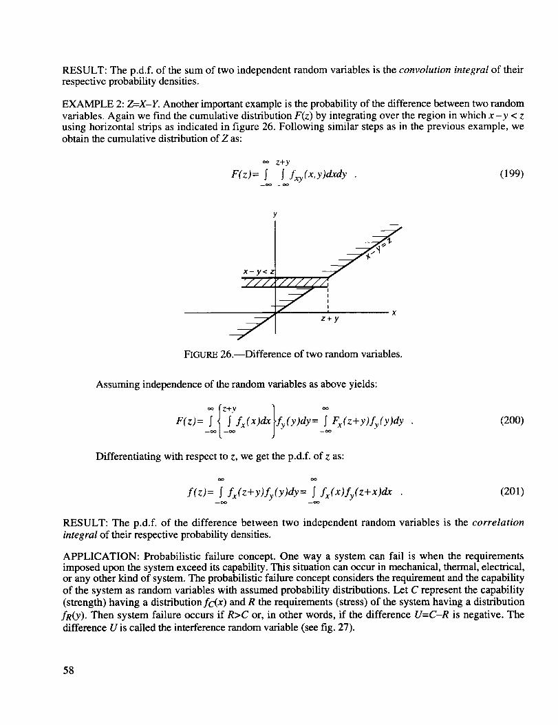
RESULT: The p.d.f, of the sum of two independent random variables is the convolution integral of theirrespective probability densities.

EXAMPLE 2: Z=X-Y. Another important example is the probability of the difference between two random

variables. Again we find the cumulative distribution F(z) by integrating over the region in which x-y < zusing horizontal strips as indicated in figure 26. Following similar steps as in the previous example, weobtain the cumulative distribution of Z as:

z+y

F(z)= S I fxy(X,y)dxdy (199)--oo --_

/I///A

| xz+y

FIGURE 26.--Difference of two random variables.

Assuming independence of the random variables as above yields:

fZ+y ]

F(Z)= 21J'fx(x)dxlfy(y)dy= _'Fx(z + y) fy(y)dy

(200)

Differentiating with respect to z, we get the p.d.f, of z as:

f(z) = I fx(Z+Y)fy(y)dy = I fx(Xjfy(Z+X) dx (201)

RESULT: The p.d.f, of the difference between two independent random variables is the correlation

integral of their respective probability densities.

APPLICATION: Probabilistic failure concept. One way a system can fail is when the requirementsimposed upon the system exceed its capability. This situation can occur in mechanical, thermal, electrical,or any other kind of system. The probabilistic failure concept considers the requirement and the capability

of the system as random variables with assumed probability distributions. Let C represent the capability

(strength) having a distributionfc(x) and R the requirements (stress) of the system having a distribution

fR(Y). Then system failure occurs if R>C or, in other words, if the difference U=C-R is negative. The

difference U is called the interference random variable (see fig. 27).

58

Requirements _/_RDistribution

/_R /1c

InterferenceArea

FIGURE 27.--Interference random variable.

The cumulative distribution of U is given as:

fu+y ] oo

F(u)= L I Lfc(x)dxlfR(Y)dy= LFc(u+ Y)fR(Y)dY (202)

Therefore, the probability of failure, also called the unreliability of the system, is:

F(O)= _j,,o{_oofc(x)dx}fR(Y)dy= _jooFc(Y)fR(Y)dy (203)

In general, the integration has to be done numerically. However, if the two random variables are

normally distributed, we know that the difference of the two random variables is again normallydistributed because of the reproductive property of the normal distribution.

Introducing the normal score of the difference u, we have:

u-( lac-la R)z= t 2 2 (204)

_J_C +(Y R

The probability of failure is then given by setting u--O. By design, the probability of failure will bevery small, such that the normal score will turn out to be negative. To use the normal score as a measure of

reliability, it is therefore customary to introduce its negative value, which is caged the safety index _. It is

numerically identical with the one-sided K-factor and the above equation then becomes:

/-tc-/_R (205)_= _GC+GR2 2

The corresponding reliability can then be obtained from the normal K-factor table or using aprogram that calculates the cumulative normal distribution. A good reference book on this subject isReliability in Engineering Design by Kapur and Lamberson.

59

Method III:

This method is of particular importance for the case where we encounter linear combinations ofindependent random variables. The method uses the so-called moment generating function.

DEFINITION: Given a random variable X the moment generating function of its distribution is given by:

oo

M(t)= _,e txi p(x i ) for discrete X (206)i=1

and

M(t)= _etXf(x)dx for continuous X . (207)--oo

The moment generating function derives its name from the following moment generating property:

oo

dnM(t) - _, xnetXi p(x i) for discrete X (208)dt n i=1

and

and

dnM(t)- _xnetXf(x)dx for continuous X . (209)dt n _oo

Taking the derivatives and setting t=0 gives:

OO

dnM(O) - _x n P(Xi)= l,tn for discrete X (210)dt n i=1

C_

dnM(O)- _xnf(x)dx for continuous X . (211)

dt n _oo

Readers who are familiar with the Laplace transform will quickly notice that the moment generatingfunction for a continuous random variable X is identical with the definition of the (two-sided or bilateral)

Laplace transform if one substitutes t=-s. In fact, if one defines the moment generating function as thebilateral Laplace transformation of the probability density function, it is possible to use existing Laplacetransform tables to find the moment generating function for a particular p.d.f..

In some advanced textbooks the variable t in the moment generating function is replaced by "i t,"

where i= _--1. It is then called the characteristic function of the distribution. This measure is sometimes

necessary because certain distributions do not have a moment generating function.

Method HI makes use of the following theorem:

If XI, X2...Xn are independent random variables and Y=XI+X2+...Xn, then

60

1/

My(t)=i_=lMxi (t) (212)

EXAMPLE: The normal distribution has the moment generating function:

Mn(t )=e llt+ l cr2t2

mean

(213)

It is readily seen that the sum of k normal random variables is again a normal distribution with

lZy=_,l.t i and variance Cr2y=]_tr 2. This is called the reproductive property of the normal

distribution. Only a few distributions have this property. The Poisson distribution is another one that hasthis property.

L. Central Limit Theorem (Normal Convergence Theorem)

If X1, X2 .... Xn are independent random variables with arbitrary distributions such that

mean: E(xi)=11i , (214)

and variance: V(xi)= cri2 , (215)

then: (216)

has an approximate standard normal distribution N(0, 1) for large n. This is the basic reason for theimportance and ubiquity of the normal distribution.

APPLICATION: Normal random number generator:

12

Gauss(0,1) = N(O,1)= _, Ui(O,1)-6 (217)i=1

Summing up 12 random numbers, which are uniform over the interval (0,1), gives an easy method

and, for practical purposes, accurate standard normal random variable. It is truncated at +6 o'. The

probability of exceeding these limits is less than 2x10 -9.

M. Simulation (Monte Carlo Methods)

Simulation techniques are used under the following circumstances:

• The system cannot be analyzed by using direct and formal analytical methods.• Analytical methods are complex, time-consuming, and costly.• Direct experimentation cannot be performed.

• Analytical solutions are beyond the mathematical capability and background of theinvestigator.

61

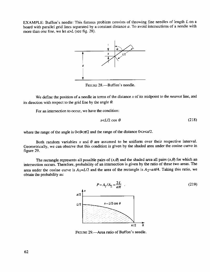
EXAMPLE: Buffon's needle: This famous problem consists of throwing fine needles of length L on a

board with parallel grid lines separated by a constant distance a. To avoid intersections of a needle with

more than one line, we let a>L (see fig. 28).

X ILl2 /

\z

FIGURE 28.--Buffon's needle.

We define the position of a needle in terms of the distance x of its midpoint to the nearest fine, and

its direction with respect to the grid line by the angle O.

For an intersection to occur, we have the condition:

x<L/2 cos 0 (218)

where the range of the angle is 0<0<rd2 and the range of the distance 0<x<a/2.

Both random variables x and 0 are assumed to be uniform over their respective interval.

Geometrically, we can observe that this condition is given by the shaded area under the cosine curve in

figure 29.

The rectangle represents all possible pairs of (x,0) and the shaded area all pairs (x,0) for which an

intersection occurs. Therefore, probability of an intersection is given by the ratio of these two areas. The

area under the cosine curve is AI=L/2 and the area of the rectangle is A2=ax/4. Taking this ratio, we

obtain the probability as:

P=A1/A 2 2L (219)=h-Y

a/2' ,x

L/2 x = L/2 cos0

tr/2 O

FIGURE 29.--Area ratio of Buffon' s needle.

62

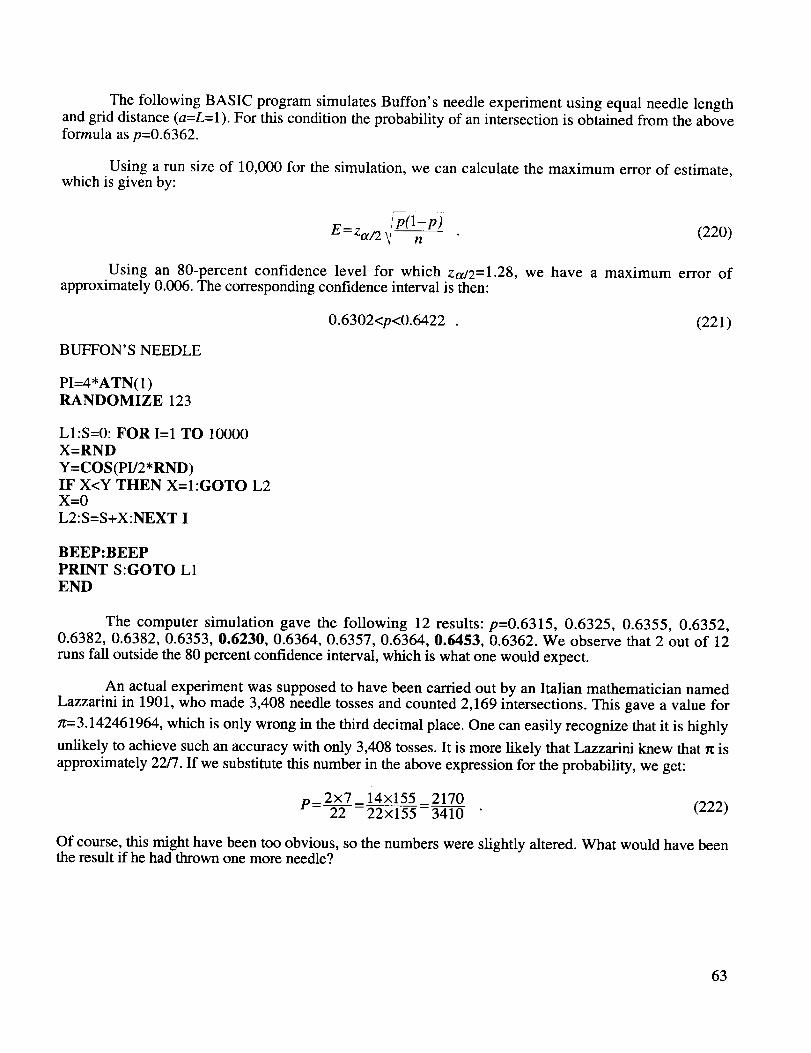
The following BASIC program simulates Buffon's needle experiment using equal needle lengthand grid distance (a=L= 1). For this condition the probability of an intersection is obtained from the aboveformula as p=0.6362.

Using a run size of 10,000 for the simulation, we can calculate the maximum error of estimate,which is given by:

/p(1-p)E = za/2 _ n (220)

Using an 80-percent confidence level for which za/2=1.28, we have a maximum error ofapproximately 0.006. The corresponding confidence interval is then:

0.6302<p<0.6422 . (221)

BUFFON'S NEEDLE

PI=4*ATN(1)RANDOMIZE 123

LI:S=0: FOR I=1 TO 10000

X=RND

Y=COS(PI/2*RND)IF X<Y THEN X=I:GOTO L2X=0

L2:S=S+X:NEXT I

BEEP:BEEP

PRINT S:GOTO L1

END

The computer simulation gave the following 12 results: p=0.6315, 0.6325, 0.6355, 0.6352,0.6382, 0.6382, 0.6353, 0.6230, 0.6364, 0.6357, 0.6364, 0.6453, 0.6362. We observe that 2 out of 12

runs fall outside the 80 percent confidence interval, which is what one would expect.

An actual experiment was supposed to have been carded out by an Italian mathematician namedLazzarini in 1901, who made 3,408 needle tosses and counted 2,169 intersections. This gave a value for

tr=3.142461964, which is only wrong in the third decimal place. One can easily recognize that it is highly

unlikely to achieve such an accuracy with only 3,408 tosses. It is more likely that Lazzarini knew that _z is

approximately 22/7. If we substitute this number in the above expression for the probability, we get:

p=2X7 14x155 2170 (222)22 -22×155-3410

Of course, this might have been too obvious, so the numbers were slightly altered. What would have beenthe result if he had thrown one more needle?

63

III. STATISTICS

A. Estimation Theory

The concepts of probability theory presented in the preceding chapters begin with certain axioms (aself-evident fact that itself is not proved, but which is the basis of all other proofs) and derive probability

laws for compound events. This is a deductive process. In statistics we are dealing with the inverse

process, which is an inductive one: given certain observations, we want to draw conclusions concerning

the underlying population. The study of such inferences is called statistical inference. Probability looks

at the population and predicts a sample. Statistics looks at the sample and predicts the population.

1. Random Sample

In order that conclusions drawn from statistical inference are valid, it is necessary to choose

samples that are representative of the population. The study of sampling methods and concomitant

statistical analysis is called the design of experiments.

One can easily see that it is often difficult to get a random sample. For example, if we are after arandom sample of people, it is not good enough to stand on a street corner and select every 10th personwho passes. Many textbooks present the following classical example of a faulty sampling method. In1936, a magazine called Literary Digest sent its readers and all telephone subscribers--approximately10 million people--a questionnaire asking how they intended to vote at the forthcoming presidentialelection.

There were 2,300,000 replies, from which it was confidently predicted that the Kansas RepublicanGovernor Alfred M. Landon would be elected. As it turned out, he lost every state but Maine and Vermont

to the incumbent president Franklin D. Roosevelt.

This erroneous prediction happened because readers of this literary magazine and people who hadtelephones did not, in 1936, represent a fair, i.e., random sample of the American voters. It was especiallyrisky to overlook the enormous proportion of nonreplies.

DEFINITION: If X1, X2 ... Xn are independent and identically distributed (rid) random variables, they are

said to constitute a random sample of size n. The joint distribution of this set of random variables is:

g(x 1,x2... Xn) =f(x 1) f(x2). • .f(Xn) (223)

where f(x) is the population distribution.

The term population is used to describe the sample space (universe) from which the sample is

drawn. Some statisticians use the term parent population.

2. Statistic

A statistic is a random variable that is a function of the random variables that constitute the random

sample. The probability distribution of a statistic is called sampling distribution.

64

3. Estimator

An estimator is a statistic that is used to make a statistical inference concerning a population

parameter O:

^ A

O=@(XpX2...X n) . (224)

B. Point Estimation

The value of an estimator provides a point estimate of a population paramater 0.

1. Properties of Estimators

There are often many possible functions capable of providing estimators. In the past the choice ofan estimator was sometimes governed by mathematical expediency. With the arrival of high-speedcomputational means, this aspect is no longer as dominant as it used to be. For example, in on-line qualitycontrol the range was commonly used to estimate the dispersion of data rather than the standard deviation.

We list several desirable characteristics for good estimators as follows:

(a) Unbiasedness:

E(6)=O

(b) Consistency (asymptotically unbiased):

//mP{6-0<e}=l or lira E(O):O .?/---->e.o

(c) Efficiency: If

(225)

(226)

Var (61 ) < Var (6 2) , (227)

61 is more efficient than 6 2 if both are unbiased.

(d) Sufficiency. An estimator is sufficient if it extracts all the information in a random sample

relevant to the estimation of the population parameter 0. Mathematically expressed as the Fisher-Newman

6-factorization theorem, - 6 (Xl, x2...Xn) is sufficient if the joint p.d.f, of XI, X2...Xn can be factorizedas:

A

f(xl, x2...Xn IO)=g[ Oxl, x2 • ..Xn I O]h(xl, x2 ...Xn) (228)

where g depends on Xl, x2...Xn only through 6 and h is entirely independent of 0.

EXAMPLE 1: Let X1, X2...Xn be normally distributed. By setting/z=01 and o'2=02 and _0=(01, 02), wehave:

65

)n n ]f(Xl,X2...X n I0)= 1 expI_ l___y_ (xi_O1)2\,,"2a'O2 [_ "_2 j=l "

(229)

But

so that

n /1

Y_ (xj -01 )2 = y_ (xj __)2 +n(2_O1 )2j=l j=l

f(xl,x2...x n I0_)=\,"--- z [. "'2 j=l " "_'2

It follows that X, Y2(X i -X') 2 is sufficient for 0=(01, 02).k y=l -

EXAMPLE 2: Consider the uniform p.d.f.:

f(x)=_forO<x<O

=0otherwise

(230)

(231)

(232)

where 0 is to be estimated on the basis of n independent observations. We want to prove that the statistic

=max (Xl, x2...Xn) is a sufficient estimator of the parameter 0.

SOLUTION: It can be shown that the cumulative distribution function of O is

F6(x)=(_) n for 0<x<O (233)

nxn-1

and, therefore, the p.d.f, of O is f_(x)- On

X2...Xn is , which may be factored as

for 0<x< O. Therefore, since the joint p.d.f, of XI,

(_)n_(nxnq) 1- ,---_j nx__ 1 , or f(xl, x2.. Xn I O)=g[6(xi,x2...Xn I0)] h (x 1, x2...Xn)(234)

as was to be shown. It is seen that the right-hand side of this expression has the desired product form such

that the first term is a p.d.f, of the statistic O and the second term does not depend on the parameter 0.

(e) Mean square error (MSE). The MSE of an estimator is defined as the expected value of the

square of the deviation of the estimator from the parameter O being estimated. It can be shown that the

MSE is equal to the variance of the estimator plus the square of its bias:

66

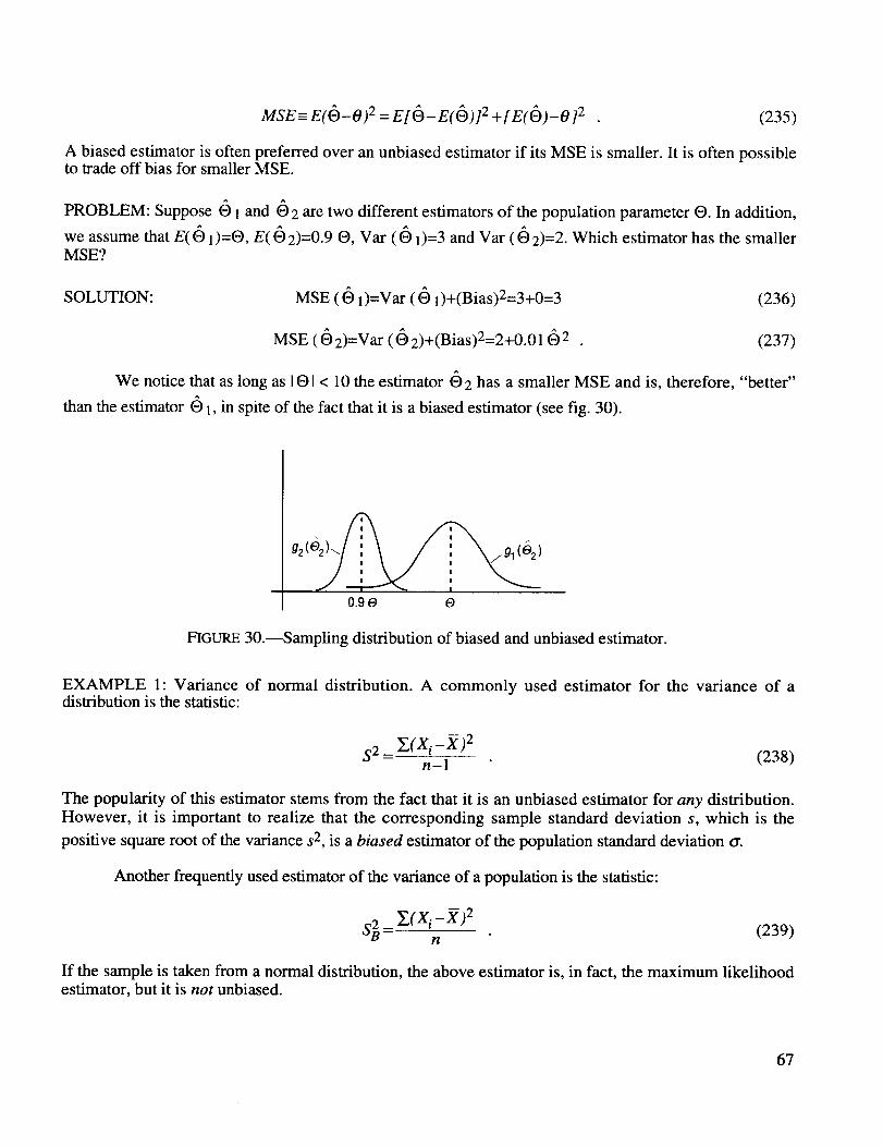
MSE = E((9-O) 2 = El6-E(_D)I 2 +[E((9)-O] 2 (235)

A biased estimator is often preferred over an unbiased estimator if its MSE is smaller. It is often possibleto trade off bias for smaller MSE.

PROBLEM: Suppose (9 1 and 6 2 are two different estimators of the population parameter O. In addition,

we assume that E( 6 1)=O, E( 6 2)=0.9 O, Var ( 6 1)=3 and Var ( 6 2)=2. Which estimator has the smallerMSE?

SOLUTION: MSE ((_ 1)=Var (6 l)+(Bias)2=3+0=3 (236)

MSE ( 6 2)=Var (6 2)+(Bias)2=2+0.01 O 2 (237)

We notice that as long as 1(91 < 10 the estimator (_2 has a smaller MSE and is, therefore, "better"

than the estimator (_ 1, in spite of the fact that it is a biased estimator (see fig. 30).

g2

FIGURE 30.--Sampling distribution of biased and unbiased estimator.

EXAMPLE 1: Variance of normal distribution. A commonly used estimator for the variance of adistribution is the statistic:

S2 _ ]_(Xi- "X)2n-1 (238)

The popularity of this estimator stems from the fact that it is an unbiased estimator for any distribution.

However, it is important to realize that the corresponding sample standard deviation s, which is the

positive square root of the variance s 2, is a biased estimator of the population standard deviation tr.

Another frequently used estimator of the variance of a population is the statistic:

82 _ ]_( X i __)2 (239)n

If the sample is taken from a normal distribution, the above estimator is, in fact, the maximum likelihoodestimator, but it is not unbiased.

67

TheMSEof thetwoestimators,whencalculatedfor anormaldistributionwith variance0"2, is:

20. 4 MSE(s2 )= (2n-l) 0.4MSE(s2)=-ffZ-(_I and n2 (240)

It can be readily verified that the MSE of the biased estimator is smaller than that of the unbiased estimator

for all sample sizes n. For a sample size of n=5, the MSE of the unbiased estimator is 39 percent higherthan that of the biased one.

EXAMPLE 2: Binomial parameter p. As a particular interesting example we compare two estimators

available for the parameter p of the binomial distribution. The unbiased estimator of this parameter is:

/3u=_ (241)

with x being the number of successes and N the number of trials. This is sometimes called the "natural"estimator and is, coincidentally, also the maximum likelihood estimator. The other biased estimator is theBayesian estimator obtained by using a uniform prior distribution and is given by:

x+l (242)&

,.,, PqIt can be shown that the variance of the unbiased estimator is Vat tPu ) =--ff and the variance of the

Bayesian estimator Vat (fib) = Npq Clearly the variance of the biased estimator is smaller than the(N+2)2 •

unbiased one. To obtain the MSE we need to determine the bias of the Bayesian estimator. Its value is

given by:

1-2p (243)Bias= N+2

Figure 31 shows the absolute value of the bias of the estimator as a function of the parameter p.

It is seen that the bias is zero for p=0.5 and is a maximum for p----&_l.Theoretically, the MSE of thebiased estimator is smaller than that of the unbiased one for:

N (244)Pq> 4(2N+1)

68

JBiasl

1N+2

p

FIGURE 31.--Estimator bias as a function of parameter.

For N---)oo, the critical value for p=0.854, implying that for greater values the unbiased estimatorshould be preferred because of its smaller MSE.

However, as the following BASIC Monte Carlo program demonstrates, the Bayesian estimator

will always be better for the practical case regardless of the value of p. The discrepancy between thetheoretical case and the real case stems from the fact that the theoretical variance of both estimators

becomes very small for high values of the parameter p. As a consequence, the bias term becomes dominantand flits the inequality in favor of the unbiased estimator.

'BINOMIAL ESTIMATOR (4/2/92)

BEGIN:

INPUT"N=",N

INPUT"P=",PRANDOMIZE 1 2 3

'HERE STARTS THE MONTE CARLO RUN WITH N= 100

L2:EB=0:EC=0: FOR R=I TO 100

'THE NEXT 5 LINES ARE THE BERNOULLI TRIALS

S=0:FOR B=I TO NU=RND

IF U<=P THEN X=I:GOTO L1X=0

L1 :S=S+X:NEXT B

'CALCULATION OF MSE

PC=X/N:PB=(X+I)/(N+2)EC=EC+(PC-P)^2:EB=EB+(PB-P)^2

NEXT R: BEEP:BEEP

PRINT EC,EBGOTO L2

69

Sample run: N=5; p=0.90

MSE

MSE

A

(Pu) =53.16, 52.20, 53.16, 54.12, 50.28

A

(Pb) =40.28, 39.69, 40.28, 40.87, 38.52

It is seen that the MSE of the Bayesian binomial estimator is always smaller than that of theclassical estimator.

2. Methods of Point Estimation

There are three methods of point estimation that will be discussed:

• Method of (matching) Moments (Karl Pearson, 1894)• Method of Maximum Likelihood (R.A. Fisher, 1922)

• Method of Least Squares (C.F. Gauss, 1810).

(a) Method of Moments. The k th sample moment is defined by:

_x/k , where n=sample size . (245)mk n

The k th population moment is defined by:

/2"k= _xk f (x)dx (246)

The method of moments consists of equating the sample moment and the population moment,

which means we set m_ =/2_. In general, this leads to k simultaneous (nonlinear) algebraic equations in

the k unknown population parameters.

EXAMPLE: Normal distribution:

Therefore:

From this follows:

/2_=# and #_ =0"2+# 2 (247)

]_Xi and 0-2 +[22 :--]_x2 (248)/2 =--n-- n

_t=_=ly_xi

"2 .2 l{_'_2_nX2)=lZ(xi__)20- =a =n_Lai

(249)

70

(b) Method of Maximum Likelihood. The likelihood function of a random sample is defined by:

L(O)=f(x 1, x2 ... Xn; 0) (250)

The method of maximum likelihood maximizes the likelihood function with respect to the

parameter 0. Statistically speaking, this means that the maximum likelihood estimator maximizes theprobability of obtaining the observed data.

EXAMPLE: Normal distribution:

n

/ /n0.2 _ 1 20 "z i=1 (251)L ( Ct, 0.2) = i=lI-IN(xi" ct' )- a _Tr2_ e

Partial differentiation of the "log-likelihood" function g = gn L with respect to/1 and 0-2 yields:

0g 1

OCt - j2 Y_(xi-Ct)=O (252)

=-_+ I--I---K(Xi--Ct)2 =0z 20.z 20-_ .

(253)

Solving for the mean Ct and the variance 0-2 we get:

_t=l y.xi=Y and 6.2= l--Z(xi-_)2=S 2n

(254)

It is interesting to observe that the method of moments and the method of maximum likelihood giveidentical estimators for a normally distributed random variable. This is, of course, not so in general.

Note that:

• The maximum likelihood estimators are often identical with those obtained by the method ofmoments.

• The set of simultaneous equations obtained by the method of likelihood is often more difficult tosolve than the one for the method of moments.

• Maximum likelihood estimators, in general, have better statistical properties than the estimatorsobtained by the method of moments.

Invariance Property

If O is a maximum likelihood estimator of the parameter 0, then g(O) is also a maximum

likelihood estimator of g(O). For example, if 6.2 is a maximum likelihood estimator of the variance tx2,

then its square root 6. is a maximum likelihood estimator of the standard deviation 0-; i.e.,

6.: _1 Y_(Xi --X') 2 (255)

71

(c) Method of Least Squares. The method of least squares is used in multivariate analyses likeregression analysis, analysis of variance (ANOVA), response surface methodology, etc. The least-squaremethod can be used to estimate the parameters of a two-parameter distribution by transforming thecumulative distribution to a straight line, using a probability scale and performing a least-square-curve fit

to this line. In general, this is a rather unwieldly process unless the cumulative distribution can be obtainedin closed form such as the Weibull distribution.

3. Robust Estimation

Over the last 2 decades statisticians have developed so-called robust estimation techniques. Theterm "robust" was coined by the statistician G.E.P. Box in 1963. In general, it refers to estimators that are

relatively insensitive to departures from idealized assumption, such as normality, or in case of a smallnumber of data points that are far away from the bulk of the data. Such data points are also referred to as"outliers." Original work in this area dealt with the location of a distribution.

An example of such a robust estimator is the so-called trimmed mean. In this case, the trimming

portions are 10 or 20 percent from each end of the sample. By trimming of this kind, one removes theinfluence of extreme observations so that the estimator becomes more robust to outliers. (The reader might

be familiar with the practice of disregarding the highest and the lowest data points for computing athleticscores.) A less severe method consists of allocating smaller weights to extreme observations in order toreduce the influence of any outliers. This leads to what is called a "Winsorized" mean. Further information

on this subject matter can be found in Data Analysis and Regression, by Mosteller et al., and in Robust

Statistics: The Approach Based on Influence Functions by Hampel et al.

Outliers. At some time or another, every engineer engaged in statistical data analysis will beconfronted with the problem of outliers. Upon examination of the data, it appears that one or moreobservations are too extreme (high, low, or both) to be consistent with the assumption that all data comefrom the same population. There is no problem when it is possible to trace the anomalous behavior tosome assignable cause, such as an experimental or clerical error. Unfortunately this is the exception ratherthan the rule. In the majority of the cases one is forced to make a judgment about the outliers, whether ornot to include them, or whether to make some allowance on some compromise basis. Clearly it is wrong to

reject an outlier simply because it seems highly unlikely or to conclude that some error in reading aninstrument must have happened. In fact, in the history of science, attention given to anomalousobservations has often led to startling new discoveries. For example, the discovery of nuclear fissioninvolved enormous energy levels which were originally considered to be outliers. This temptation must be

strongly resisted. Once one starts handpicking the data, the sample becomes a biased one. The best rule,therefore, is to never reject an outlier unless an assignable cause has been positively identified.

What actually is needed is some objective statistical method to decide whether or not an outlier doesin fact exist. However, since the outlier problem is by its very nature concerned with the tails of adistribution, any statistical method will be very sensitive to departures from the assumed distribution. Dueto the mathematical difficulties involved, the majority of statistical research has so far dealt with the normaldistribution.

One of the earliest methods for dealing with outliers is known as Chauvenet's criterion (1863).

This rather strange proposal is stated as follows: If in a sample of size n the probability of the deviation ofthe outlier from the mean is smaller than 1/2n, the outlier is to be rejected.

Chauvenet's criterion is based on the concept of the characteristic extreme (largest or smallest

value), which was introduced by Richard V. Mises. The characteristic largest value Un is defined as:

nR( un)=n[1-F( un) ]= l (256)

72

wheren=sample size and

Pr(u<Un)=F(un) is the cumulative distribution function.

Pr(u>Un)=R(un)=l - F(un) . (257)

Accordingly, we expect that on the average, one observation in a sample of size n will exceed the value Un.

Similarly, the characteristic smallest value Ul is defined as:

nF(ul)=l (258)

The number of observations n corresponding to the characteristic largest or smallest value is also called the

return period T(un) or T(ul), respectively. This means we expect the maximum or minimum value to

occur once in a return period. The concept of the return period is sometimes used in engineering design.

Note that if an event has a probability of p, then the mathematical expectation for this event to

happen is defined by E=n p. Therefore, if we set E=I, we can make the statement that it takes 1/p trials onthe average for the event to happen once.

It is important to notice that the characteristic extreme value is a population parameter and not arandom variable. The characteristic largest value is found by solving the above equation for F(un):

F(un)= 1-1/n . (259)

According to Chauvenet's criterion, data points will be rejected as outliers if they fall above the criticalvalue defined by:

nR(unC)=n[1-F(unC)] =1 (260)

In other words, we expect that in a sample of size n, on the average "one-half" observation will

exceed the critical value Unc. In the case where data points are rejected, the parameters of the distribution

are recalculated without the rejected values. If we know the distribution of the population from which thesample is drawn, we can determine this critical value from the relation

F(un c) = 1- _n (261)/

For a normal distribution N(0, 1) we obtain:

u_0 = 1- 1_1000

n=50 Fu_o = 1 - 1/100 u_0 = K0.99 = 2.33 (262)

n=500 Fu_o 0 = 1- 1_100 u_00 = 1- 1_1000 . (263)

It is seen that when applied to a normal distribution, Chauvenet's criterion is absolutelymeaningless. At most, one could use this criterion to flag suspicious data points in a sample.

73

Return periods are often chosen to be equal to twice the service life of a structure when maximumloads or winds are fitted to an extreme value distribution (Gumbel distribution). It is seen that the basis for

the factor two is actually Chauvenet's criterion.

C. Sampling Distributions

The probability distribution of a statistic S is called its sampling distribution. If, for example, theparticular statistic is used to estimate the mean of a distribution, then it is called the sampling distribution ofthe mean. Similarly we have sampling distributions of the variance, the standard deviation, the median, therange, etc. Naturally, each sampling distribution has its own population parameters such as the mean,standard deviation, skewness, kurtosis, etc. The standard deviation of a sampling distribution of the

statistic S is often called its standard error as.

1. Sample Mean

If the random variables XI, X2...Xn constitute a random sample of size n, then the sample mean is

defined as:

X= _'Xi (264)n

Note that it is common practice to also apply the term statistic to values of the corresponding randomvariable. For instance, to calculate the mean of a set of observed data, we substitute into the formula:

= Zxi (265)n

where the xi are the observed values of the corresponding random variables.

First, let us state some general results that hold for arbitrary distributions with mean p and

variance o_-:

• Infinite population:

-- -- .2 _ 0 .2 (266)E(X)=l.t_=12 and Var(X)=o_- n

• Finite population of size N:

-- 2 0.2 N-nE(X)=Ia_=Iz and Var(X)=a_=--ff-x-ffL-T_ 1 (267)

Note that the information embodied in the sample is minimally affected by the proportion that the samplebears relative to its population and essentially determined by the sample size itself. In fact, the finite

population correction factor is usually ignored if the sample size does not exceed 5 percent of thepopulation.

74

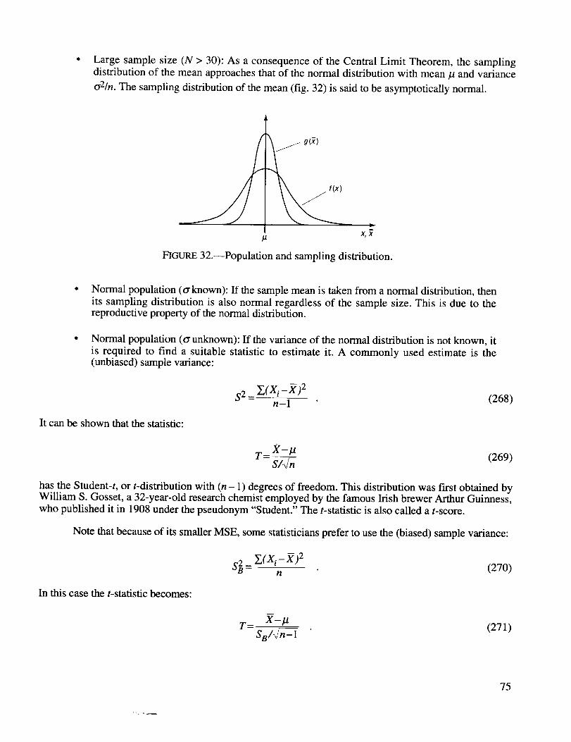
Largesamplesize (N > 30): As a consequenceof the CentralLimit Theorem,the samplingdistributionof themeanapproachesthatof thenormaldistributionwith mean/.tandvariancecr2/n. The sampling distribution of the mean (fig. 32) is said to be asymptotically normal.

x,_

FIGURE 32.--Population and sampling distribution.

Normal population (a known): If the sample mean is taken from a normal distribution, then

its sampling distribution is also normal regardless of the sample size. This is due to thereproductive property of the normal distribution.

Normal population (tr unknown): If the variance of the normal distribution is not known, it

is required to find a suitable statistic to estimate it. A commonly used estimate is the(unbiased) sample variance:

s a _ Z(xi _ ,2)2n-1 (268)

It can be shown that the statistic:

w

T= X-IaS/_ (269)

has the Student-t, or t-distribution with (n- 1) degrees of freedom. This distribution was first obtained byWilliam S. Gosset, a 32-year-old research chemist employed by the famous Irish brewer Arthur Guinness,

who published it in 1908 under the pseudonym "Student." The t-statistic is also called a t-score.

Note that because of its smaller MSE, some statisticians prefer to use the (biased) sample variance:

S2 _ Z(Xi __)2n (270)

In this case the t-statistic becomes:

T- X-/.tSB/_-Z_ (271)

75

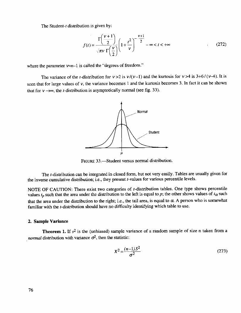
TheStudent-tdistributionis givenby:

F -2-f(t) = 1 + _ oo < t < +oo (272)

where the parameter v=-n-1 is called the "degrees of freedom."

The variance of the t-distribution for v >2 is v/(v-1) and the kurtosis for v >4 is 3+6/(v-4). It is

seen that for large values of v, the variance becomes 1 and the kurtosis becomes 3. In fact it can be shown

that for v ---)oo, the t-distribution is asymptotically normal (see fig. 33).

Normal

ent

FIGURE 33.--Student versus normal distribution.

The t-distribution can be integrated in closed form, but not very easily. Tables are usually given for

the inverse cumulative distribution; i.e., they present t-values for various percentile levels.

NOTE OF CAUTION: There exist two categories of t-distribution tables. One type shows percentile

values tp such that the area under the distribution to the left is equal to p; the other shows values of ta such

that the area under the distribution to the right; i.e., the tail area, is equal to t_. A person who is somewhat

familiar with the t-distribution should have no difficulty identifying which table to use.

2. Sample Variance

Theorem 1. If s 2 is the (unbiased) sample variance of a random sample of size n taken from a

normal distribution with variance o -2, then the statistic:

X2 _ (n-l) S 2 (273)o-2

76

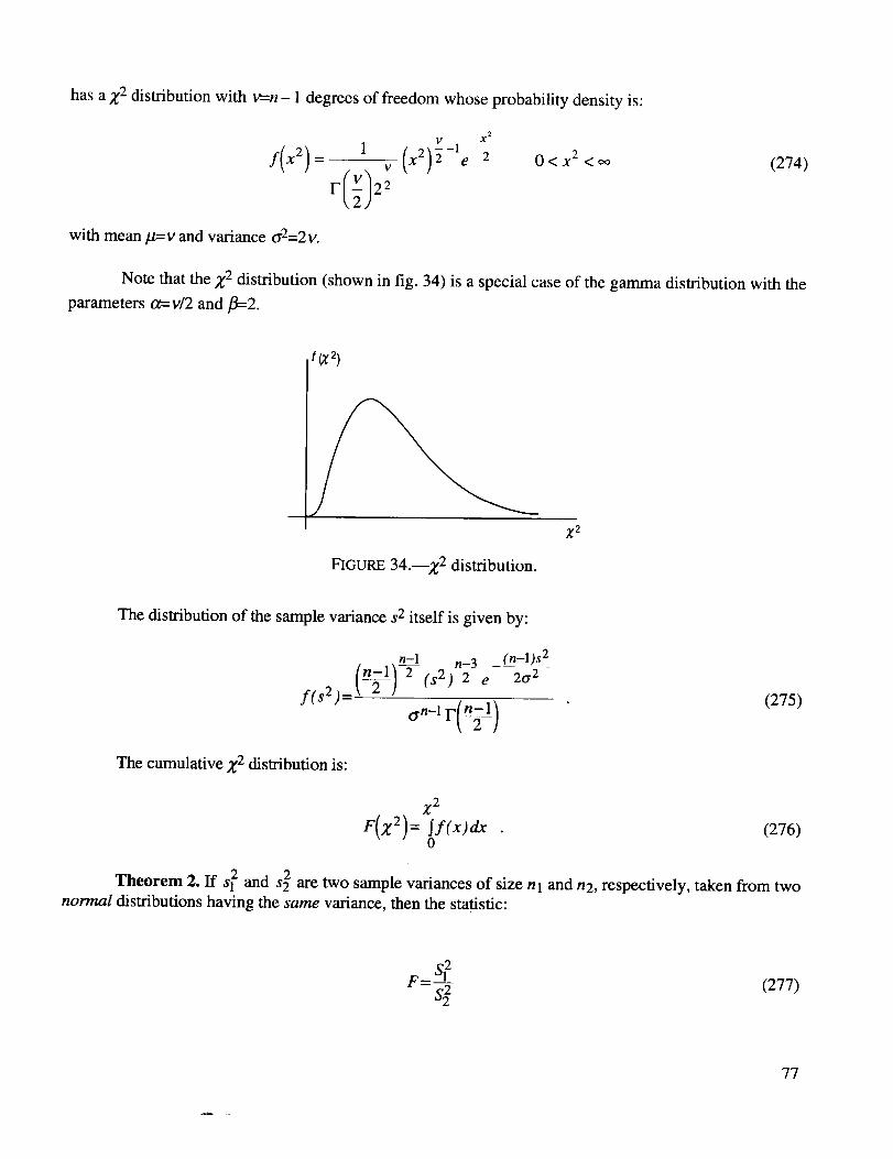
hasaZ 2 distribution with v=-n - 1 degrees of freedom whose probability density is:

1 v X 2 2- - 0<X2<OO (274)

with mean/t=v and variance o'2=2 v.

Note that the Z 2 distribution (shown in fig. 34) is a special case of the gamma distribution with the

parameters a=v/2 and/3=2.

t(z 2)

FIGURE 34.--Z2 distribution.

X 2

The distribution of the sample variance s 2 itself is given by:

n-1 n-3

(n--l) 2 (s2) 2f(s2)-

a n-1 F(n_)

(n-1)s 2

-- e 2cr2

(275)

The cumulative Z 2 distribution is:

Z 2

F(Z2) = Sf(x)dx0

(276)

Theorem 2. If s 2 and s 2 are two sample variances of size nl and n2, respectively, taken from twonormal distributions having the same variance, then the statistic:

(277)

77

hasaFisher'sF-distribution with:

vl=nl-1 and v2=n2-1 degrees of freedom. (278)

The F-distribution is also known as the variance-ratio distribution:

g(F) =

v 1

rIVl+V211v ) v12,20<F<oo (279)

(Vl +7 2 )

with:V 2

mean /a= v--_ forv2>2

variance o -2= 2v2(vl+v2-2) forv2>4v I (v 2 -2) 2 (v 2 -4)

(280)

(281)

REMARK: The F-distribution is related to the beta function as follows: IfX has a beta distribution with

vl _)_parameters _=_- and fl= , then the statistic:

F= v2X (282)v 1(1- X)

has an F-distribution with Vl and v2 degrees of freedom.

3. Sample Standard Deviation

For a sample size n>30 taken from an arbitrary population, the sampling distribution of the

standard deviation S can be approximated by a normal distribution with:

0"2 (283)las =0" and o-2_ 2(n-l)

The standard normal random variable is then:

S-0- (284)Z=0-1_

78

D. Interval Estimation

Interval estimates are used to assess the accuracy or precision of estimating a population

parameter 0. They are defined by the confidence (fiducial) intervals within which we expect a population

parameter 0 to be located.

Two-sided confidence interval:

P ( (_L<0< _) u)=l-a •

One-sided confidence interval:

- Lower confidence interval:

- Upper confidence limit:

(285)

P ( OL<O)= 1-a (286)

P(O< 0 u)=l-a . (287)

The confidence interval is a random variable because the confidence limits (upper and lower endpoints) arerandom variables.

The probability (1-a) that the confidence interval contains the true population parameter 0

is called the degree of confidence or the confidence (level). The corresponding interval is called a

(I-a) 100-percent confidence interval. The quantity tx is called the significance coefficient.

An analogy given by N.L. Johnson and F.C. Leone in Statistics and Experimental Design statesthat: "A confidence interval and statements concerning it are somewhat like the game of horseshoe tossing.The stake is the parameter in question. (It never moves regardless of some sportsmen's misconceptions.)The horseshoe is the confidence interval. If out of 100 tosses of the horseshoe one tings the stake 90 timeson the average, he has 90-percent assurance (confidence) of tinging the stake. The parameter, just like thestake, is the constant. At any one toss (or interval estimation) the stake (or parameter) is either enclosed ornot. We make a probability statement about the variable quantities represented by the positions of the armsof the horseshoe."

1. Mean

To obtain a two-sided confidence interval for the mean, we use the t-statistic, which is given by:

m

X-#

T= S/_/_ with v=-n - 1 (288)

and establish the following double inequality

P[-ta/. 2 < T < ta/2 ]= 1-or (289)

or

79

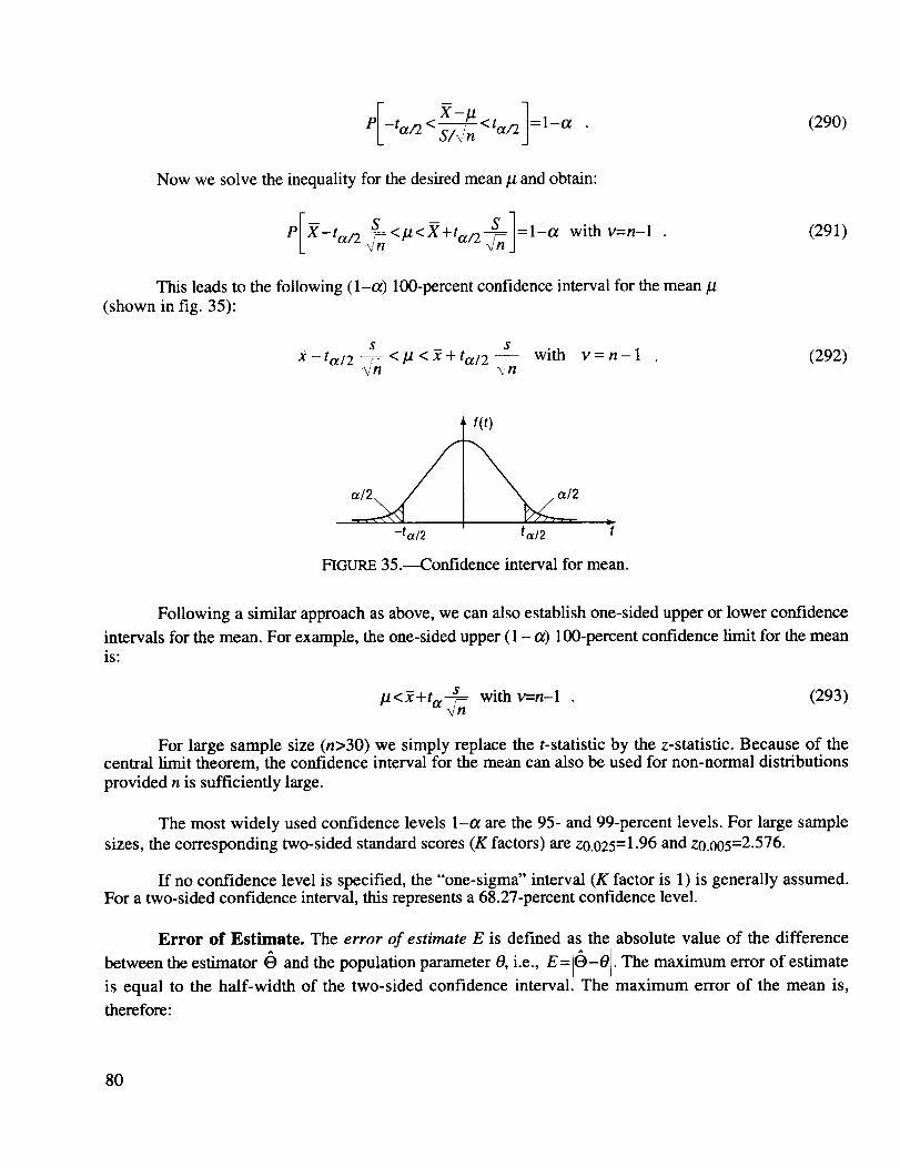
X-/2

Now we solve the inequality for the desired mean/2 and obtain:

This leads to the following (l-a) 100-percent confidence interval for the mean/2

(shown in fig. 35):

S S

_ - ta12 T < /2 < _ + tod2 __ with V = n -1_,'n _ n

(290)

(291)

(292)

-ta/2

, t(t)

tal2

FIGURE 35.---Confidence interval for mean.

Following a similar approach as above, we can also establish one-sided upper or lower confidence

intervals for the mean. For example, the one-sided upper (1 - a) 100-percent confidence limit for the meanis:

S

la<2+ta---_n n with v----n-1(293)

For large sample size (n>30) we simply replace the t-statistic by the z-statistic. Because of thecentral limit theorem, the confidence interval for the mean can also be used for non-normal distributions

provided n is sufficiently large.

The most widely used confidence levels 1-a are the 95- and 99-percent levels. For large sample

sizes, the corresponding two-sided standard scores (K factors) are z0.025=1.96 and z0.005=2.576.

If no confidence level is specified, the "one-sigma" interval (K factor is 1) is generally assumed.For a two-sided confidence interval, this represents a 68.27-percent confidence level.

Error of Estimate. The error of estimate E is defined as the absolute value of the difference

between the estimator O and the population parameter 0, i.e., E= 8-0. The maximum error of estimate

is equal to the half-width of the two-sided confidence interval. The maximum error of the mean is,

therefore:

80

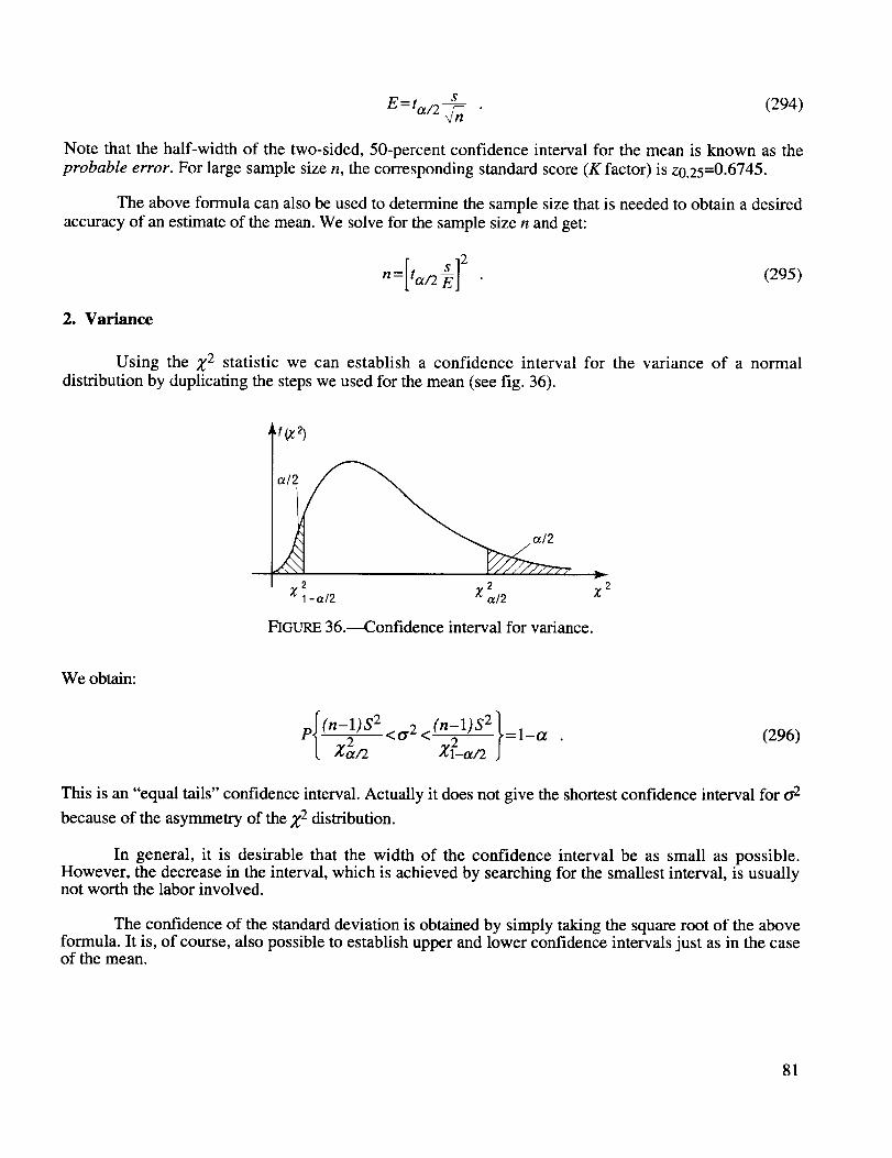
s (294)E = ta/2 _/n

Note that the half-width of the two-sided, 50-percent confidence interval for the mean is known as the

probable error. For large sample size n, the corresponding standard score (K factor) is z0.25=0.6745.

The above formula can also be used to determine the sample size that is needed to obtain a desired

accuracy of an estimate of the mean. We solve for the sample size n and get:

n=[ta/2 _] 2 (295)

2. Variance

Using the Z 2 statistic we can establish a confidence interval for the variance of a normal

distribution by duplicating the steps we used for the mean (see fig. 36).

,t (z2)

Z 2 Z 21-a/2 a/2

r

Z 2

FIGURE 36.--Confidence interval for variance.

We obtain:

p_(n-1) $2 < (n-l) $2[ Z2/2 <a 2 Z2__a/2 '=l-a

(296)

This is an "equal tails" confidence interval. Actually it does not give the shortest confidence interval for o.2

because of the asymmetry of the Z 2 distribution.

In general, it is desirable that the width of the confidence interval be as small as possible.However, the decrease in the interval, which is achieved by searching for the smallest interval, is usuallynot worth the labor involved.

The confidence of the standard deviation is obtained by simply taking the square root of the aboveformula. It is, of course, also possible to establish upper and lower confidence intervals just as in the caseof the mean.

81

3. Standard Deviation

If the sample size is large (n>30), the sampling distribution of the standard deviation S of an

arbitrary distribution is nearly normal, and we can use its sampling distribution to establish a (l-a) 100-

percent confidence interval as:

s <or< s (297)l+za/2/_/2(n-1) 1-za/2/_ 2_(n-1)

4. Proportion

(a) Approximate Confidence Limits. When the sample size n is large, we can construct an

approximate confidence interval for the binomial parameter p by using the normal approximation to the

binomial distribution. To this end we observe that the estimate /3= X of the population parameter p has ann

asymptotically normal distribution with mean E(/3)=p and variance Var(/3)= -p-q . The equivalent

z-score is:

Z: _-E(_) /3_p where q=l-p . (298)

_/Var (P) Pq

The two-sided large sample (l-a) 100-percent confidence interval is then given by:

P - P (299)-Zot l 2 < < Zotl 2fp(1-p)

_r n

This is a quadratic equation in the parameter p and could be solved to obtain the approximate

confidence interval for p. But for the sake of simplicity, we make the further approximation of substituting

/3 in the expression for the variance of /3 appearing in the denominator of the above equation. The

approximate confidence interval is then determined by:

r

Pt/3-zot/2_-PQ-<P</3+Z_/2_-_-t=I-a.(3oo)

It is again of interest to find the sample size n that is necessary to attain a desired degree of

accuracy for the estimate of the binomial parameter p. It is:

(301)

Note that if no information is available for the value of p, we set p=l/2 to obtain the maximum samplesize.

82

EXAMPLE: Supposewe want to establisha 95-percent confidencethat the error doesnot exceed3 percent.Thenwemusthaveasamplesizeof:

=1[ 1.96 / 2 = 1,067 (302)n 4_0.03}

(b) Exact Confidence Limits. In reliability work the concern is usually with one-sided

confidence limits. For a large sample size n one can, of course, establish one-sided limits by the samemethod that was used above for the one-sided confidence limits of the mean. However, it is not verydifficult to find the exact limits by resorting to available numerical algorithms. These are based upon thefollowing mathematical relationships.

(1) The Upper Confidence Limit. PU is determined from the solution to the followingequation:

_ I_lpk(1--pu)n-k:o(,k=0

(303)

This equation can be solved for the upper limit PU by using the equivalency of the binomial sum

and the beta integral and then equating the beta integral to the F-distribution. The result is:

(x+l) Fa (Vl'V2) 2(x+l)andv 2 2(n x) (304)Pu = with v 1 = = - .(n-x)+(x + l) Fa (Vl,V2)

(2) The Lower Confidence Limit. PL is determined from the solution to the followingequation:

n

]L (lk)p k (l-PL)n-k=ak=x \ ./

(305)

and solved for the unknown lower limit Pu in terms of the F-distribution:

x with Vl=2(n-x+l) and v2=2x . (306)PL - x+(n--x+l)F a (V1,V 2)

NOTE: Comparing these confidence limits for the binomial parameter p with the analogous Bayesian

confidence limits, it is noticed that the upper limit corresponds to a prior beta distribution with _=1 and

fl=0, whereas the lower limit is obtained by setting these prior parameters to _ and fl=l.

(3) Two-Sided Confidence Limits. The two-sided confidence limits are obtained by simply

replacing the significance coefficient ct by tz/2 for the corresponding upper and lower limits.

E. Tolerance Limits

Tolerance limits establish confidence intervals for a desired percentile point _p where the subscript

p indicates the proportion to the left of the percentile point of a distribution. They are used in designspecifications ("design allowables") and deal with the prediction of a future single observation. The

83

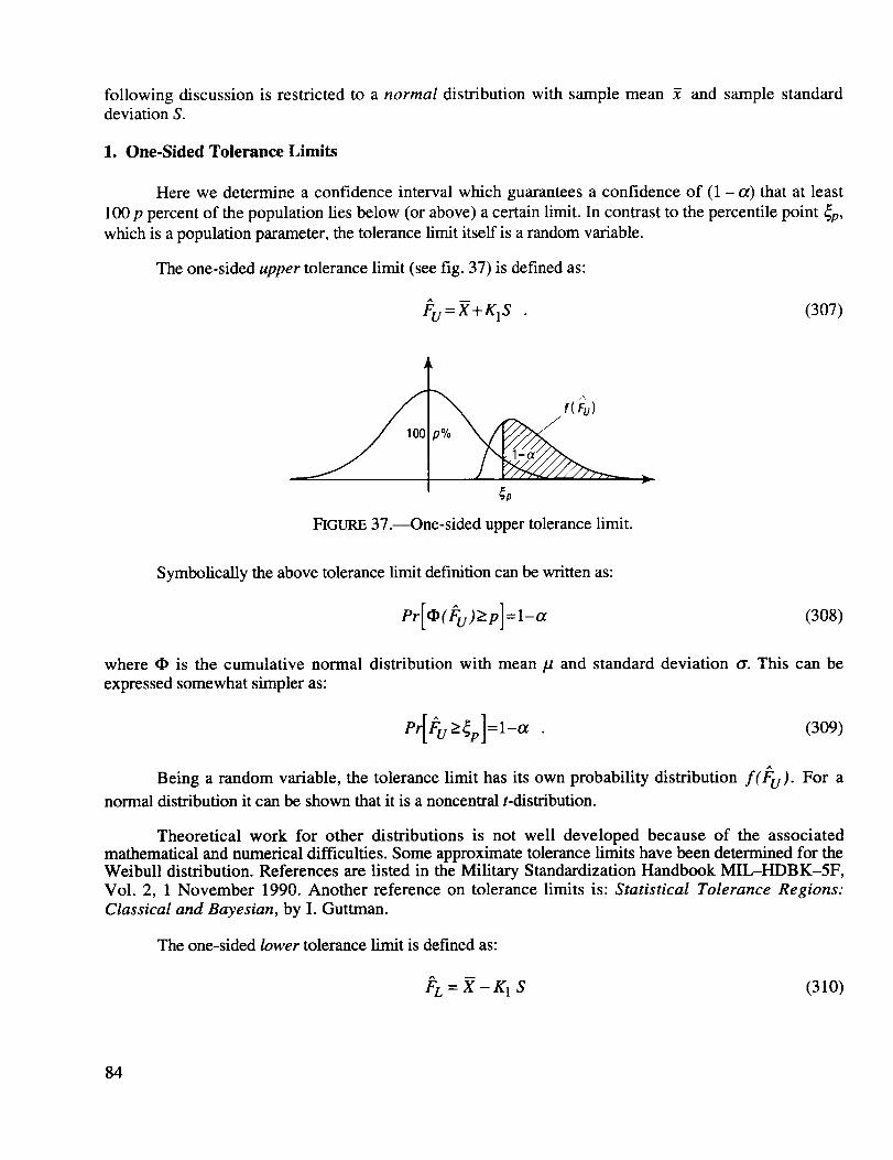
following discussion is restricted to a normal distribution with sample mean Y and sample standarddeviation S.

1. One-Sided Tolerance Limits

Here we determine a confidence interval which guarantees a confidence of (1 - a) that at least

100 p percent of the population lies below (or above) a certain limit. In contrast to the percentile point _p,

which is a population parameter, the tolerance limit itself is a random variable.

The one-sided upper tolerance limit (see fig. 37) is defined as:

_'u = 2"+K1S (307)

p% _,_

dp

FIGURE 37.---One-sided upper tolerance limit.

Symbolically the above tolerance limit definition can be written as:

Pr[dP([:U)>_p]=l-a (308)

where • is the cumulative normal distribution with mean/z and standard deviation dr. This can be

expressed somewhat simpler as:

Pr[Fu>_p]:l-oc (309)

Being a random variable, the tolerance limit has its own probability distribution f(Fu)" For a

normal distribution it can be shown that it is a noncentral t-distribution.

Theoretical work for other distributions is not well developed because of the associatedmathematical and numerical difficulties. Some approximate tolerance limits have been determined for theWeibull distribution. References are listed in the Military Standardization Handbook MIL-HDBK-5F,Vol. 2, 1 November 1990. Another reference on tolerance limits is: Statistical Tolerance Regions:

Classical and Bayesian, by I. Guttman.

The one-sided lower tolerance limit is defined as:

/_L = _ - K1 S (310)

84

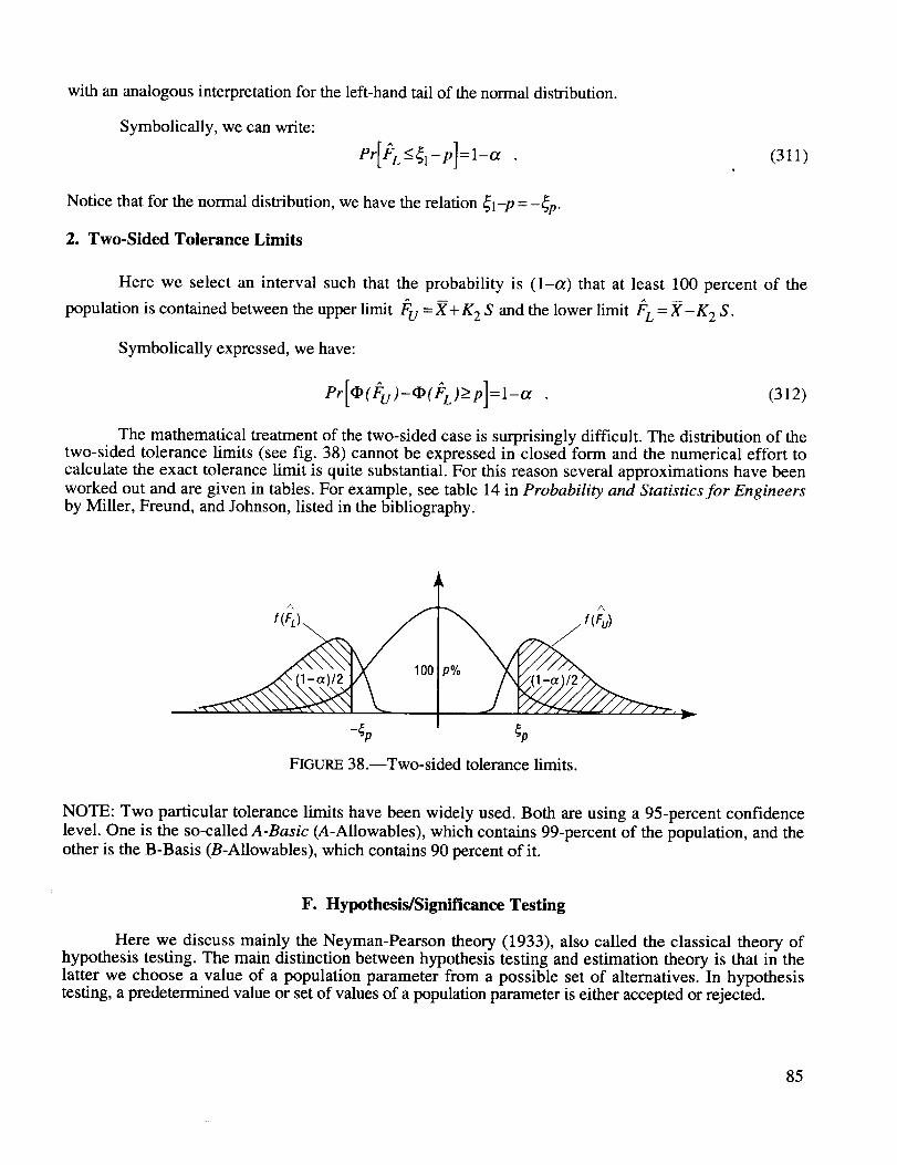
withananalogousinterpretationfor theleft-handtail of thenormaldistribution.

Symbolically,wecanwrite:

Pr[F L <_l-P]=l-a

Notice that for the normal distribution, we have the relation _I-P = -_p.

2. Two-Sided Tolerance Limits

(311)

Here we select an interval such that the probability is (1-00 that at least 100 percent of the

population is contained between the upper limit b'u = X"+ K 2 S and the lower limit ['L = X'- K 2 S.

Symbolically expressed, we have:

Pr[O(Fu)-_(FL)>P]=I-ot (312)

The mathematical treatment of the two-sided case is surprisingly difficult. The distribution of thetwo-sided tolerance limits (see fig. 38) cannot be expressed in closed form and the numerical effort tocalculate the exact tolerance limit is quite substantial. For this reason several approximations have been

worked out and are given in tables. For example, see table 14 in Probability and Statistics for Engineersby Miller, Freund, and Johnson, listed in the bibliography.

FIGURE 38.--Two-sided tolerance limits.

NOTE: Two particular tolerance limits have been widely used. Both are using a 95-percent confidence

level. One is the so-called A-Basic (A-Allowables), which contains 99-percent of the population, and theother is the B-Basis (B-Allowables), which contains 90 percent of it.

F. Hypothesis/Significance Testing

Here we discuss mainly the Neyman-Pearson theory (1933), also called the classical theory ofhypothesis testing. The main distinction between hypothesis testing and estimation theory is that in thelatter we choose a value of a population parameter from a possible set of alternatives. In hypothesistesting, a predetermined value or set of values of a population parameter is either accepted or rejected.

85

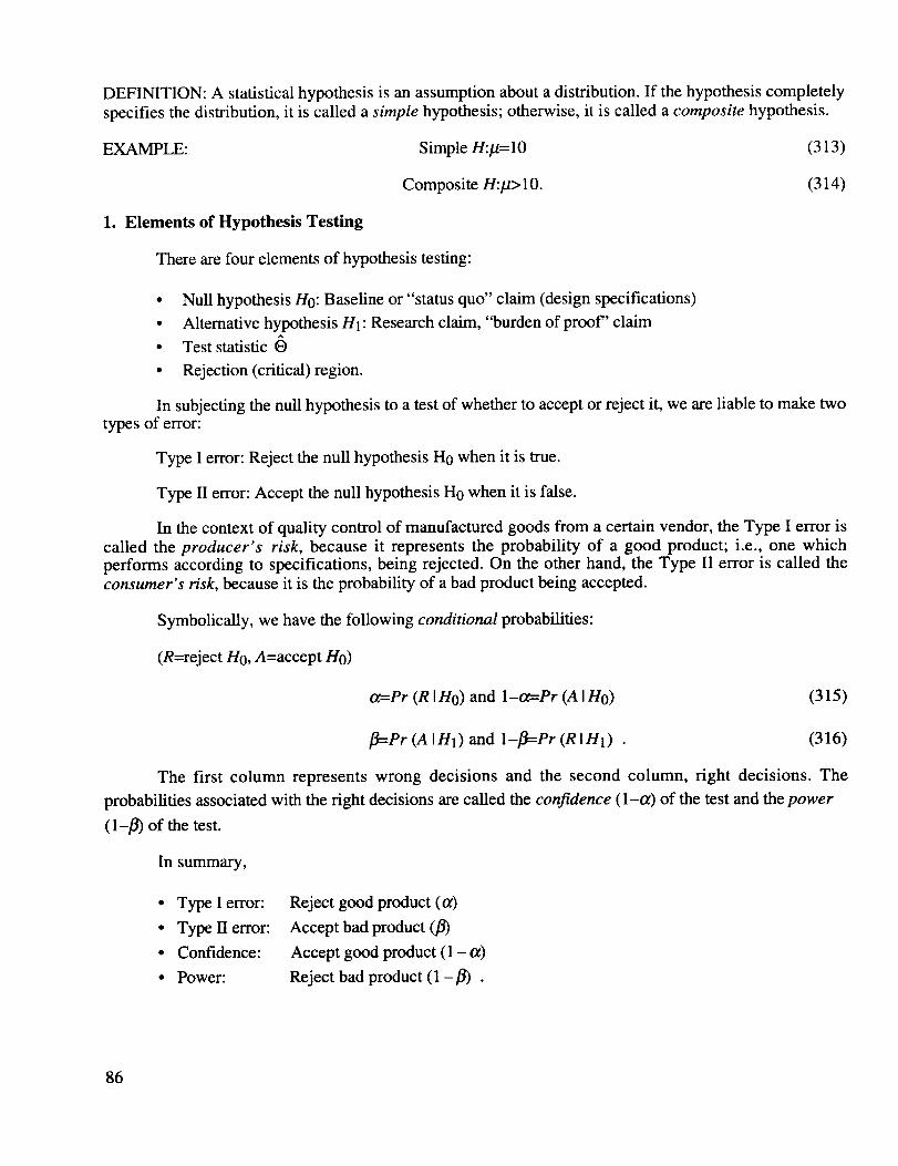
DEFINITION:A statisticalhypothesisis anassumptionaboutadistribution.If thehypothesiscompletelyspecifiesthedistribution,it is calleda simple hypothesis; otherwise, it is called a composite hypothesis.

EXAMPLE: Simple H:#=10 (313)

Composite H:/z> 10. (314)

1. Elements of Hypothesis Testing

There are four elements of hypothesis testing:

• Null hypothesis H0: Baseline or "status quo" claim (design specifications)

• Alternative hypothesis HI: Research claim, "burden of proof" claim^

• Test statistic O

Rejection (critical) region.

In subjecting the null hypothesis to a test of whether to accept or reject it, we are liable to make twotypes of error:

Type I error: Reject the null hypothesis H0 when it is true.

Type II error: Accept the null hypothesis H0 when it is false.

In the context of quality control of manufactured goods from a certain vendor, the Type I error is

called the producer's risk, because it represents the probability of a good product; i.e., one whichperforms according to specifications, being rejected. On the other hand, the Type II error is called theconsumer's risk, because it is the probability of a bad product being accepted.

Symbolically, we have the following conditional probabilities:

(R=reject H0, A=accept H0)

¢z=Pr (R IHo) and 1-a=Pr (A IHo) (315)

fl=Pr (A IH1) and 1-fl=Pr (R IH1) . (316)

The first column represents wrong decisions and the second column, right decisions. The

probabilities associated with the right decisions are called the confidence (l-ix) of the test and the power

(l-t) of the test.

In summary,

• Type I error:

• Type 11error:

• Confidence:

• Power:

Reject good product (a)

Accept bad product (fl)

Accept good product (1 - ix)

Reject bad product (1 -t) .

86

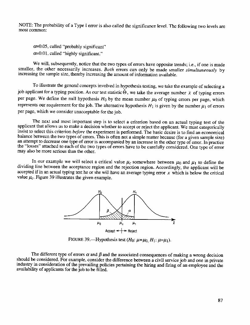
NOTE:Theprobabilityof aTypeI erroris alsocalledthesignificancelevel.Thefollowing two levelsaremostcommon:

a_=0.05, called "probably significant"

t_=0.01, called "highly significant."

We will, subsequently, notice that the two types of errors have opposite trends; i.e., if one is made

smaller, the other necessarily increases. Both errors can only be made smaller simultaneously byincreasing the sample size, thereby increasing the amount of information available.

To illustrate the general concepts involved in hypothesis testing, we take the example of selecting a

job applicant for a typing position. As our test statistic 8, we take the average number 2 of typing errors

per page. We define the null hypothesis H0 by the mean number P0 of typing errors per page, which

represents our requirement for the job. The alternative hypothesis H 1 is given by the number Pl of errors

per page, which we consider unacceptable for the job.

The next and most important step is to select a criterion based on an actual typing test of theapplicant that allows us to make a decision whether to accept or reject the applicant. We must categoricallyinsist to select this criterion before the experiment is performed. The basic desire is to find an economical

balance between the two types of errors. This is often not a simple matter because (for a given sample size)an attempt to decrease one type of error is accompanied by an increase in the other type of error. In practicethe "losses" attached to each of the two types of errors have to be carefully considered. One type of errormay also be more serious than the other.

In our example we will select a critical value/.tc somewhere between #0 and #1 to define the

dividing line between the acceptance region and the rejection region. Accordingly, the applicant will be

accepted if in an actual typing test he or she will have an average typing error 2 which is below the criticalvalue/.tc. Figure 39 illustrates the given example.

H0 H1

I

/'tO /2c /21

Accept_ Reject

FIGURE 39.--Hypothesis test (H0:/.t=/.t0, HI"//=/11).

X

The different type of errors t_ and fl and the associated consequences of making a wrong decision

should be considered. For example, consider the difference between a civil service job and one in privateindustry in consideration of the prevailing policies pertaining the hiring and firing of an employee and theavailability of applicants for the job to be filled.

87

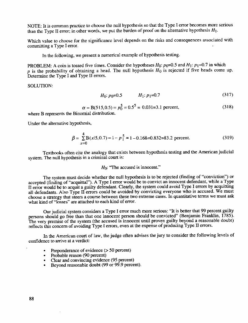
NOTE: It is commonpracticeto choosethenull hypothesissothattheTypeI errorbecomesmoreseriousthantheTypeII error; in other words, we put the burden of proof on the alternative hypothesis H1.

Which value to choose for the significance level depends on the risks and consequences associated with

committing a Type I error.

In the following, we present a numerical example of hypothesis testing.

PROBLEM: A coin is tossed five times. Consider the hypotheses H0:p0=0.5 and HI: pl=0.7 in which

p is the probability of obtaining a head. The null hypothesis H0 is rejected if five heads come up.Determine the Type I and Type II errors.

SOLUTION:

H0:p0=0.5 HI: p1=0.7 (317)

o_ = B(515,0.5) = p05 = 0.55 = 0.031=3.1 percent,

where B represents the Binomial distribution.

(318)

Under the alternative hypothesis,

4

/3 = _B(x15,0.7) = 1 - p 5 = 1 -0.168=0.832=83.2 percent. (319)x=0

Textbooks often cite the analogy that exists between hypothesis testing and the American judicial

system. The null hypothesis in a criminal court is:

H0: "The accused is innocent."

The system must decide whether the null hypothesis is to be rejected (finding of "conviction") oraccepted (finding of "acquittal"). A Type I error would be to convict an innocent defendant, while a TypeII error would be to acquit a guilty defendant. Clearly, the system could avoid Type I errors by acquittingall defendants. Also Type II errors could be avoided by convicting everyone who is accused. We mustchoose a strategy that steers a course between these two extreme cases. In quantitative terms we must askwhat kind of "losses" are attached to each kind of error.

Our judicial system considers a Type I error much more serious: "It is better that 99 percent guiltypersons should go free than that one innocent person should be convicted" (Benjamin Franklin, 1785).The very premise of the system (the accused is innocent until proven guilty beyond a reasonable doubt)reflects this concern of avoiding Type I errors, even at the expense of producing Type II errors.

In the American court of law, the judge often advises the jury to consider the following levels ofconfidence to arrive at a verdict:

• Preponderance of evidence (> 50 percent)• Probable reason (90 percent)• Clear and convincing evidence (95 percent)• Beyond reasonable doubt (99 or 99.9 percent).

88

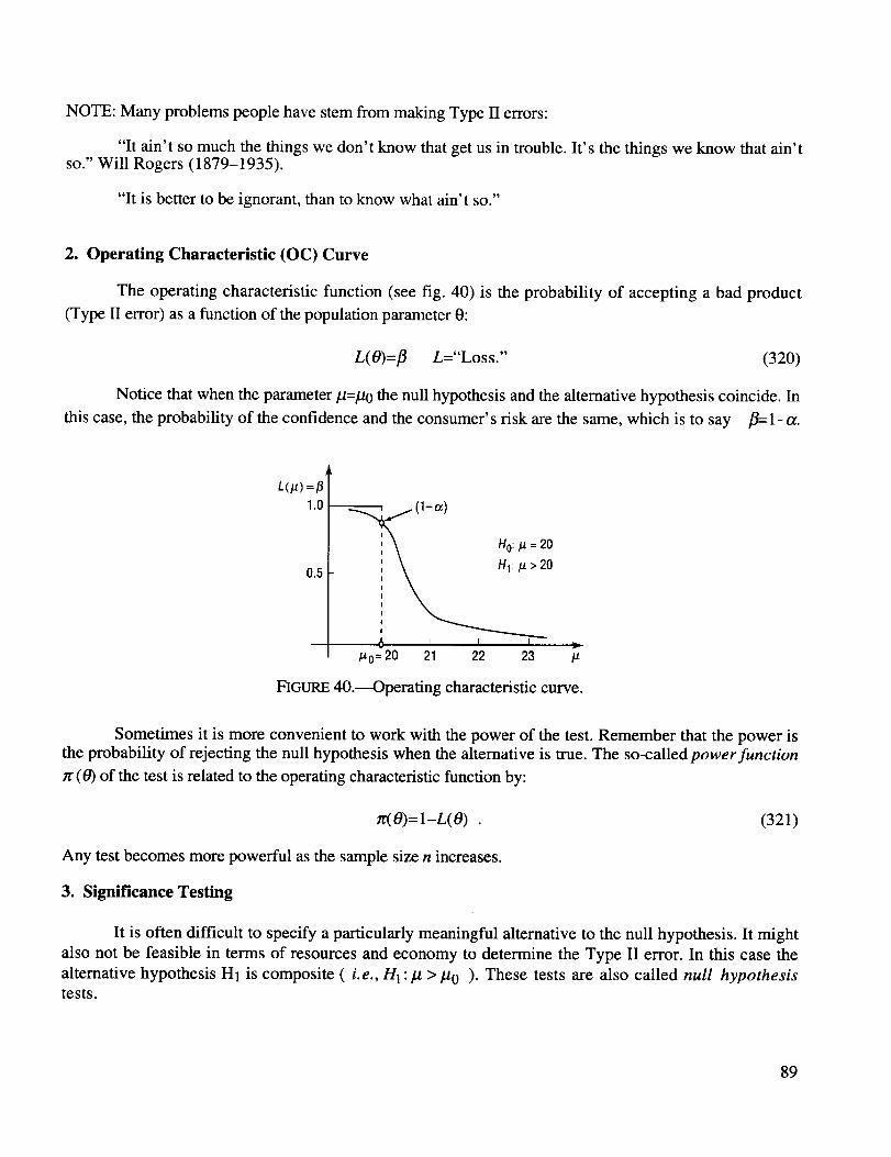
NOTE:Manyproblemspeoplehavestemfrom makingTypeII errors:

"It ain't somuchthethingswedon't knowthatgetusin trouble.It's thethingsweknow thatain'tso."Will Rogers(1879-1935).

"It is betterto beignorant,thanto knowwhatain't so."

2. Operating Characteristic (OC) Curve

The operating characteristic function (see fig. 40) is the probability of accepting a bad product

(Type II error) as a function of the population parameter 0:

t.(o)=/3 L:"Loss." (320)

Notice that when the parameter/.t=/zo the null hypothesis and the alternative hypothesis coincide. In

this case, the probability of the confidence and the consumer's risk are the same, which is to say fl=l-a.

0.5

Ho:/z=20

HI:/z>20

6 J J I j,p,o= 20 21 22 23 /.z

FIGURE 40.----Operating characteristic curve.

Sometimes it is more convenient to work with the power of the test. Remember that the power isthe probability of rejecting the null hypothesis when the alternative is true. The so-called power function

r¢ (0) of the test is related to the operating characteristic function by:

7r(O)= l-L( O) . (321)

Any test becomes more powerful as the sample size n increases.

3. Significance Testing

It is often difficult to specify a particularly meaningful alternative to the null hypothesis. It might

also not be feasible in terms of resources and economy to determine the Type II error. In this case the

alternative hypothesis H1 is composite ( i.e., H 1 :/_ > #0 ). These tests are also called null hypothesistests.

89

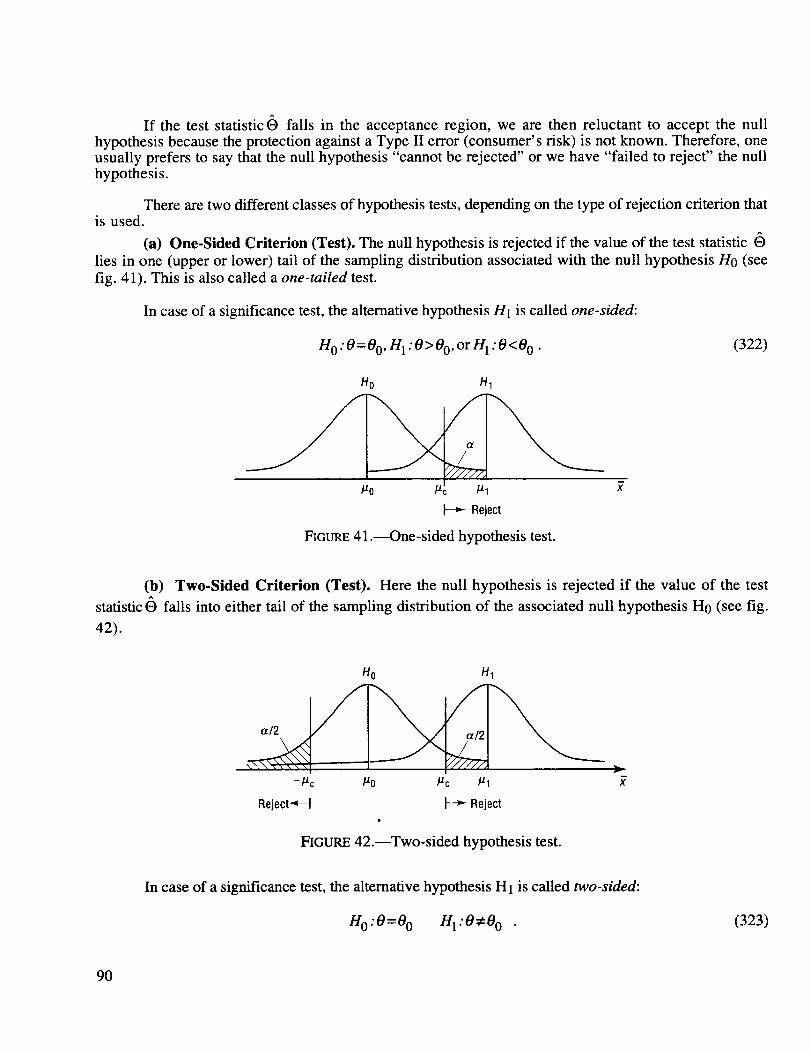
If the test statisticO falls in the acceptanceregion, we are then reluctant to acceptthe nullhypothesisbecausetheprotectionagainstaTypeII error (consumer'srisk) is notknown.Therefore,oneusuallyprefersto saythatthenull hypothesis"cannotbe rejected"or wehave"failed to reject" thenullhypothesis.

Therearetwodifferentclassesof hypothesistests,dependingonthetypeof rejectioncriterionthatis used.

(a) One-SidedCriterion (Test).Thenull hypothesisis rejectedif thevalueof theteststatisticlies in one (upperor lower) tail of thesamplingdistributionassociatedwith thenull hypothesisH0 (see

fig. 41). This is also called a one-tailed test.

In case of a significance test, the alternative hypothesis HI is called one-sided:

H 0 .'0=0 O, H 1:0>0 O, or H 1:0<0 0 . (322)

H, H 1

Reject

FIGURE 41 .---One-sided hypothesis test.

(b) Two-Sided Criterion (Test). Here the null hypothesis is rejected if the value of the test

statistic E) falls into either tail of the sampling distribution of the associated null hypothesis HO (see fig.

42).

H0

-/ac #o #c #1

Reject-_-I _ Reject

FIGURE 42.--Two-sided hypothesis test.

H1

r

In case of a significance test, the alternative hypothesis HI is called two-sided:

Ho:O=O 0 nl:O¢O 0 (323)

90

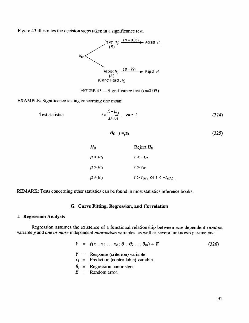
Figure43 illustratesthedecisionstepstaken in a significance test.

Reject HO:

Ho: _ (R)

Accept Ho: (/3 = ??)

(A)(CannotRejectHo)

(o_= 0.05) > Accept H1

,_ Reject H1

FIGURE 43.--Significance test (a=0.05)

EXAMPLE: Significance testing concerning one mean:

Test statistic: t=2- ,it,, , v=n-1S/\/n

(324)

H0 : #=Po (325)

H0 Reject H0

//</.to t < -te

/z >/-t0 t > ta

/z _:/t0 t > ta/2 or t < -ttx/2

REMARK: Tests concerning other statistics can be found in most statistics reference books.

G. Curve Fitting, Regression, and Correlation

1. Regression Analysis

Regression assumes the existence of a functional relationship between one dependent random

variable y and one or more independent nonrandom variables, as well as several unknown parameters:

Y

Y =

X i =

_j

E

= f(xl, x2 ... Xn; 01, 02 ... Om) + E (326)

Response (criterion) variable

Prediction (controllable) variable

Regression parametersRandom error.

91

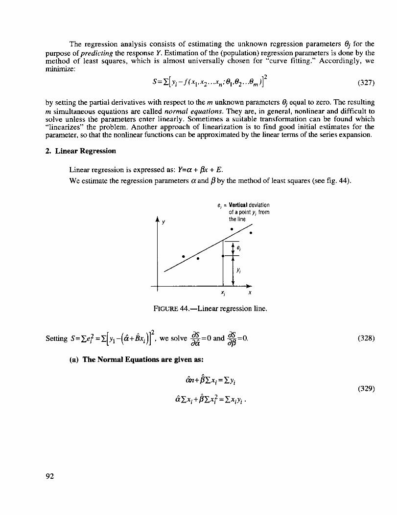
The regressionanalysisconsistsof estimating the unknown regressionparametersOj for the

purpose of predicting the response Y. Estimation of the (population) regression parameters is done by themethod of least squares, which is almost universally chosen for "curve fitting." Accordingly, weminimize:

S= _'[yi-- f (Xl,X2...Xn;Ol,O2...Om)] 2 (327)

by setting the partial derivatives with respect to the m unknown parameters 0j equal to zero. The resulting

m simultaneous equations are called normal equations. They are, in general, nonlinear and difficult tosolve unless the parameters enter linearly. Sometimes a suitable transformation can be found which"linearizes" the problem. Another approach of linearization is to find good initial estimates for theparameter, so that the nonlinear functions can be approximated by the linear terms of the series expansion.

2. Linear Regression

Linear regression is expressed as: Y=tx + fix + E.

We estimate the regression parameters a and fl by the method of least squares (see fig. 44).

Y

ei = Vertical deviation

of a point Yi fromthe line

ID,

FIGURE 44.--Linear regression line.

Setting S= Y.e2 _,[yl-( & + Bxi)]2 KS _ _9S= , we solve ff_-0 and ff_ =0.

(a) The Normal Equations are given as:

_+_,Xi=_,Y i

_ _,xi + _,x2= _,xiY i •

(328)

(329)

92

(b) Abbreviations.We next introducethefollowing standardnotation:

2 2Sxx: Y,(xi-x)2: _,x i -(_,xi) /n

Syy = _,(Yi-Y )2 = _,y2-(_,Yi )2/n (330)

Sxy = Y_(xi- x )(Yi- Y)= _xiYi-(_,xi )(YYi )/n .

(e) Least-Square Estimators. The least-square estimators are:

&= y-/_Y and/_= Sxy with E(&)=aand E(/_)= ft. (331)Xxx

3. Gauss Markov Theorem

The Gauss Markov theorem states that:

• The estimators & and/_ are unbiased.

• The estimators & and/_ have the smallest variance, i.e., they are the most efficient ones.

This theorem is independent of the probability distribution of the random variable y. The variance

o.2 of the random error E is usually estimated by:

t_2=S2=nl-_2_,[yi-(dt+ffJxi)] 2 • (332)

The division n- 2 is used to make the estimator for tr2 unbiased. The term Se is called the standarderror of the estimate.

The computational form of _2 is:

2_Syy- Sxyn-2 (333)

4. Normal Regression Model

The normal regression model is expressed as:

f(Yilxi)- t7_2_ exp- Yi for -_ < Yi < e_ (334)

The maximum likelihood estimators for a, fl, and o.2 are identical to the least square estimators

except that _.2 has the divisor n instead of (n - 2).

93

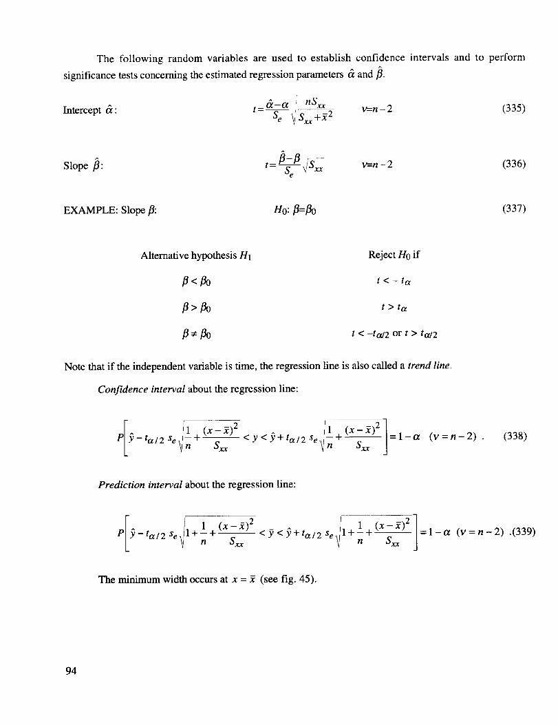
The following randomvariables are used to establishconfidenceintervals and to performsignificancetestsconcerningtheestimatedregressionparameters& and/_.

SIntercept & : t = °:S--a ,' n-xx v=-n - 2 (335)

e \iSxx +.22

Slope ]_: t = flSe--fl\/Sxx v=n-2 (336)

EXAMPLE: Slope fl: H0:fl=fl0 (337)

Alternative hypothesis H1 Reject H0 if

fl < flO t < - ta

fl > flO t > ta

fl ;_ flO t < -ta/2 or t > ta/2

Note that if the independent variable is time, the regression line is also called a trend line.

Confidence interval about the regression line:

_ r (x - X)2I1 (x-2) 2 Se_'l+P Y-ta/2Se_tn+ <Y<Y+ta/2 Sxx=l-t_ (v = n - 2) . (338)

Prediction interval about the regression fine:

I i 1 (x - .2) 2 f 1 (x - .2)2 7P Y-ta/2 Se\ll +- +n S-x_ < Y < Y+ ta /2 Se _t l+-+n S-xx J=l-a (V = n - 2) .(339)

The minimum width occurs at x = ff (see fig. 45).

94

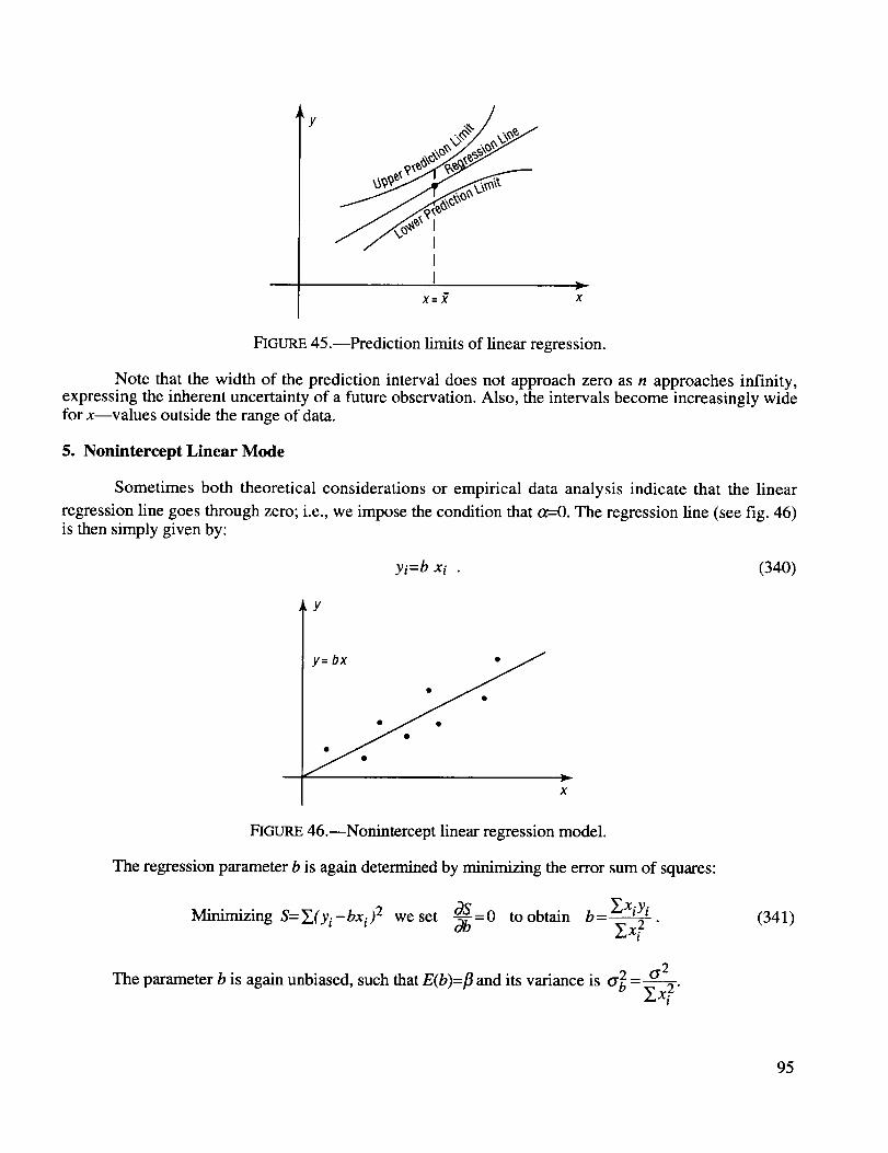
Y

I

X=X X

FIGURE 45 .--Prediction limits of linear regression.

Note that the width of the prediction interval does not approach zero as n approaches infinity,expressing the inherent uncertainty of a future observation. Also, the intervals become increasingly widefor x--values outside the range of data.

5. Nonintereept Linear Mode

Sometimes both theoretical considerations or empirical data analysis indicate that the linear

regression line goes through zero; i.e., we impose the condition that t_=0. The regression line (see fig. 46)is then simply given by:

yi=b xi • (340)

y

x

FIGURE 46.--Nonintercept linear regression model.

The regression parameter b is again determined by minimizing the error sum of squares:

we b- _'xiYitgS _ to obtainMinimizing S=_.,(Yi-bxi) 2 set _--0 - Y'x 2

(3r2

The parameter b is again unbiased, such that E(b)=fl and its variance is 0 .2 = 2£x2.

(341)

95

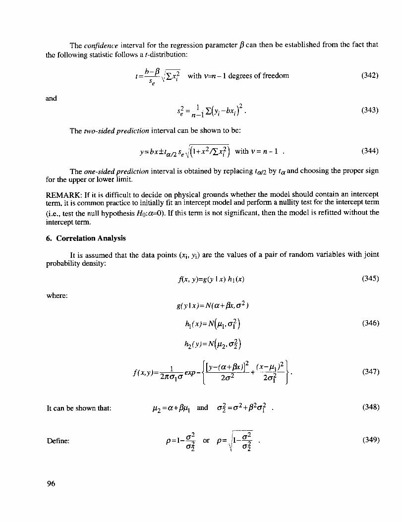
The confidence interval for the regression parameter fl can then be established from the fact that

the following statistic follows a t-distribution:

t = b_efl \jY_x 2 with v=n- 1 degrees of freedom (342)

and

S2 = nl-_l _,(Yi -bxi )2 . (343)

The two-sided prediction interval can be shown to be:

(l+x2/_x 2) with v= n-1 (344)Y= bx+ta/2 Se _i'

The one-sided prediction interval is obtained by replacing tat2 by ta and choosing the proper sign

for the upper or lower limit.

REMARK: If it is difficult to decide on physical grounds whether the model should contain an interceptterm, it is common practice to initially fit an intercept model and perform a nullity test for the intercept term

(i.e., test the null hypothesis Ho:a=O). If this term is not significant, then the model is refitted without the

intercept term.

6. Correlation Analysis

It is assumed that the data points (xi, Yi) are the values of a pair of random variables with joint

probability density:

f(x, y)=g(y Ix) hi(x) (345)

where:

g(y Ix)=N(ot+flx, a 2)

h2(Y):N(tl2,cr2 )

1 exp_J[Y-(°t+flx)] 2 (x-Ill)2 \

f(x,y)- 21t0.ICr L 20"2 ÷ _ J"

(346)

(347)

It can be shown that: #2 = 0_+_]./1 and 0"2 =0"2 +1_20"? (348)

Define:_ if2 il if2

p-1--_222 or p:_[. 0"2(349)

96

Also: and 0"2=0.2(1-p2) (350)

Then

0.1

p=K-2t_

Q(x,y) ]

f (x, y )- exp-[_ _v2(1-_p2 ) _j which is the Bivariate Normal Distribution, (351 )c

2It0.10"2 _ 1-p 2

where

Q(x)=IFX-_l I=_2pFx-& lFy-u2 l+Fy-_=121[L 0.1 .] L 0.1 ]L 0.2 .] L 0.2 J J"

(352)

o Other Regression Models

Three other regression models are polynomial, multiple, and exponential.

Polynomial regression:

Multiple regression:

Y=fl0 +_lX+fl2X2 +. ..B pxP +8.

Y= flO +_lxl +f12x2 +'''nrXr WE"

(353)

(354)

These two models are still linear regression models because they are linear in the unknown regressionparameters.

r'=x f! + e_. (355)

Using matrix notation, we can write:

S = eTe = (Y- Xfl)T(E - Xfl). (356)

Minimizing S we obtain

o3S : 2xT(y_ - Xfl)=O (357)

and

[J = (xTx)-IxTy .

The matrix C=(X T X) -1 X T is called the pseudo-inverse of X.

(358)

97

For example, if we consider the exponential model:

y = ct e _6x ,

We "linearize" it by taking logarithims of both sides, to obtain:

gny = gno_ + _oc.

(359)

(360)

8. Sample Correlation Coefficient

Sample correlation coefficient scattergrams are shown in figure 47. The correlation coefficient

allows a quantitative measure of how well a curve describes the functional relationship between the

dependent and independent variables.

• gO • s2=z(yj-_,i) 2Unexplained Variation

Y

6

. $2 =_ (Yi-.17) 2Total Variation

FIGURE 47.--Sample correlation coefficient (scattergrams).

Decomposition of the Total Sum of Squares. The derivation of the correlation coefficient is

based on the fact that the total sum of squares of the deviation of the individual observations Yl (i=1, 2 ...

n) from the mean y can be decomposed in two parts if the regression model is a polynomial of the form:

_=b 0+b 1x+b 2x 2+...b kx k • (361)

The error sum of squares is then given as:

n n

S=i_=lE2=i_=l(Yi-Yi)2

tl

=i_=l[Yi-(bo+blx+b2x2+...bkxk)] 2 "

(362)

98

Partial differentiation with respect to the regression parameters/3i yields the normal equations:

ff_ffO=-2Y[Yi-(bo +blX +...bk xk )]=O_ Y_Ei=O

-_11 =-OS2Yf[yi -(bo +bl x +...b k x k )] xi =0 _ _Eixi=O

ff_ffk =-2_[Yi-(bo +bl X+...bk xk )]xk=O=* _F.ixk=O .

Therefore:

(363)

]_ei Yi =Y_ei (b0 +bl x +...b k x k )= ]_ei + ]_ei xi +" ""_,eixk =0. (364)

This is a significant result because it reveals that the correlation between the error e and the estimate _ is

zero, or one can also say that all the information contained in the data set y has been removed.

The total sum of squares denoted by SST can then be written as:

SSW=Syy = ]_(yi--y)2=]_(yi--_+_i--_i) 2

= Y_(Yi_y)2 +Y'(Yi --Yi) 2 +2_(Yi--Y)(Yi--Yi)" (365)

The last term on the right-hand side can be seen to be zero as follows:

_(Yi-Y)(Yi-Yi)= ]_(Yi -Y)ei = YYiei-YY'_'i =0. (366)

Therefore, we have the f'mal result that the total variation can be decomposed as follows:

SST = X(Yi _y)2 = Y.(Yi _y)2 + ]_(Yi -yi)2 = SSR+SSE (367)

where SSR is the regression ("explained") sum of squares and SSE the error ("unexplained") sum ofsquares.

The coefficient of determination is the ratio of the explained variation to the total variation. Since

it is always positive, we denote it by r2:

r 2 _ E @i - y)2

E (Yi - y)2

S 2E (Yi - _)2 _ 1 - -- (368)

=1 E (Yi - _)2 - S2

Note that r2 does not depend on the units employed because of its nondimensional nature.

99

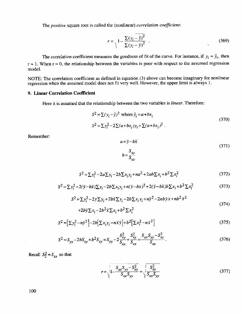
Thepositive square root is called the (nonlinear) correlation coefficient:

r

iI

r= ,Jl _(Yi - _)2 (369)

Y_(Yi _y)2

The correlation coefficient measures the goodness of fit of the curve. For instance, if Yi = Yi, then

r = 1. When r = 0, the relationship between the variables is poor with respect to the assumed regressionmodel.

NOTE: The correlation coefficient as defined in equation (3) above can become imaginary for nonlinear

regression when the assumed model does not fit very well. However, the upper limit is always 1.

9. Linear Correlation Coefficient

Here it is assumed that the relationship between the two variables is linear. Therefore:

S 2 =_(yi-_) 2 where_i =a+bx i(370)

$2 = Y_Y? - 2 Y'(a+ bxi )Yi + Y'( a+ bxi )2 "

Remember:

a=y-bY

b=SxYG

(371)

S 2 = _,y2 _2a_y i _2bY.xiy i +ha 2 +2abY_x i +b 2 y.x 2

S 2 = Zy 2 -2(y-b2)_,y i -2b_,xiY i +nfy-b_) 2 +2(y-b_)bY.x i +b 2 Y.x 2

S 2 = y.y2 _ 2yy.y i + 2b2Y_y i _ 2bY.x i Yi +ny2 _ 2nby2 +nb 2 _2

+2byZx i -2b22Zxi +b 2 £x 2

S 2 =[y.y2 _ny2 ]_ 2b[Y_xiYi_nXy]+b2[y.x 2 _nX2]

S 2 2 2

S2=Syy-2bSxy+b2Sxy=Syy-2-.. xy 4 G SxxSyy-S_'YSxx- G

Recall S 2 =Sxx so that

SxxSyy-S2xySr=_l SxxSyy = xy

(372)

(373)

(374)

(375)

(376)

(377)

100

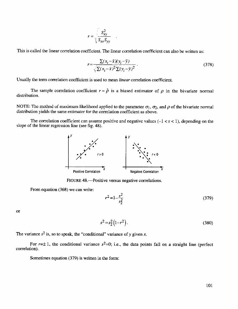
[ U! S_y

r _ i m

S Syy

This is called the linear correlation coefficient. The linear correlation coefficient can also be written as:

r = _'(xi -x)(Yi -y) (378)

_,y.( xi _ _ )2 Y_(Yi _y)2

Usually the term correlation coefficient is used to mean linear correlation coefficient.

The sample correlation coefficient r = ¢3 is a biased estimator of p in the bivariate normaldistribution.

NOTE: The method of maximum likelihood applied to the parameter 0-1, 0"2, and p of the bivariate normaldistribution yields the same estimator for the correlation coefficient as above.

The correlation coefficient can assume positive and negative values (-1 < r < 1), depending on theslope of the linear regression line (see fig. 48).

Y

XPositiveCorrelation NegativeCorrelation

x

FIGURE 48.--Positive versus negative correlations.

From equation (368) we can write:

r2=l -s_2 (379)q

or

s2=s2(1-r2). (380)

The variance s 2 is, so to speak, the "conditional" variance of y given x.

For r=+ 1, the conditional variance s2=0; i.e., the data points fall on a straight line (perfectcorrelation).

Sometimes equation (379) is written in the form:

101

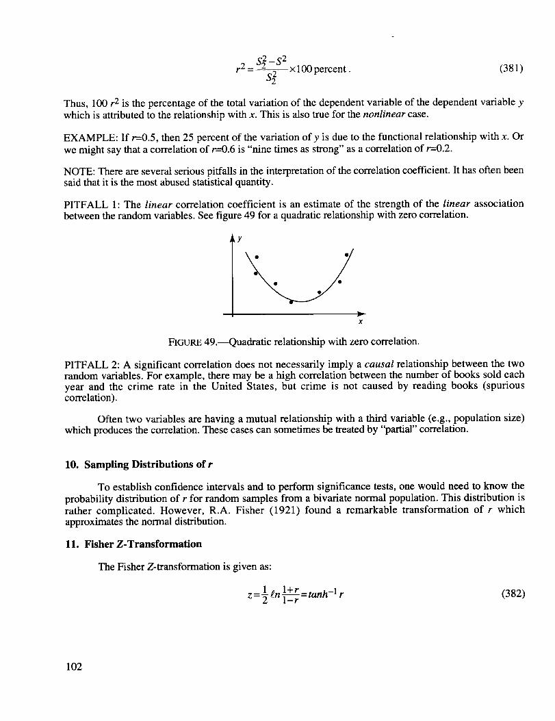
r 2 _ $2-S 2$2 xl00percent.

(381)

Thus, 100 r 2 is the percentage of the total variation of the dependent variable of the dependent variable y

which is attributed to the relationship with x. This is also true for the nonlinear case.

EXAMPLE: If r=-0.5, then 25 percent of the variation ofy is due to the functional relationship with x. Or

we might say that a correlation of r=-0.6 is "nine times as strong" as a correlation of r=0.2.

NOTE: There are several serious pitfalls in the interpretation of the correlation coefficient. It has often beensaid that it is the most abused statistical quantity.

PITFALL 1: The linear correlation coefficient is an estimate of the strength of the linear association

between the random variables. See figure 49 for a quadratic relationship with zero correlation.

x

FIGURE 49.--Quadratic relationship with zero correlation.

PITFALL 2: A significant correlation does not necessarily imply a causal relationship between the tworandom variables. For example, there may be a high correlation between the number of books sold eachyear and the crime rate in the United States, but crime is not caused by reading books (spuriouscorrelation).

Often two variables are having a mutual relationship with a third variable (e.g., population size)

which produces the correlation. These cases can sometimes be treated by "partial" correlation.

10. Sampling Distributions of r

To establish confidence intervals and to perform significance tests, one would need to know the

probability distribution of r for random samples from a bivariate normal population. This distribution is

rather complicated. However, R.A. Fisher (1921) found a remarkable transformation of r whichapproximates the normal distribution.

11. Fisher Z-Transformation

The Fisher Z-transformation is given as:

1 l+r -1z=_gn]-L--i=tanh r (382)

102

with

EXAMPLE:

CONFIDENCEINTERVAL:

_ 1. l+pIdz-_n]_ fi and tY2=nl-_3

for n>30 (383)

r=0.70 n=30 (384)

Z=0.867 ix=0.05 (385)

_'n-3 </'tz < Z+(386)

where Za/2=1.96 for 95-percent confidence:

0.867-1.966 </.t z <0.867+ 1.96_'27 _/27

0.490 </z z < 1.244

or for the correlation coefficient:

(387)

(388)

0.45 < p < 0.85 (389)

Estimates of correlation coefficients based on small sample sizes are not very reliable. For

instance, if the sample size n=20, the calculated correlation coefficient has to exceed the critical value

rc=0.377 to be significant at a=0.05.

H. Goodness-of-Fit Tests

Goodness-of-fit tests examine how well a sample of data agrees with a proposed probability

distribution. Using the language of hypothesis testing, the null hypothesis H0 is that the given data set

follows a specified distribution F(x). In most applications the alternative hypothesis H1 is very vague andsimply declares that H0 is wrong. In other words, we are dealing with significance tests in which the TypeII error or the power of the test is not known. Moreover, in contrast to the usual significance tests wherewe usually look for the rejection of the null hypothesis in order to prove a research claim, goodness-of-fit

tests actually are performed in the hope of accepting the null hypothesis H0.

To make up for the lack of existence of a well-defined alternative hypothesis, many differentconcepts have been proposed and investigated to compare the power of different tests. The result of this

quite extensive research indicates that uniquely "best" tests do not exist. There are essentially two differentapproaches to the problem of selecting a proper statistical model for a data set--probability plotting(graphical analysis) and statistical tests.

103

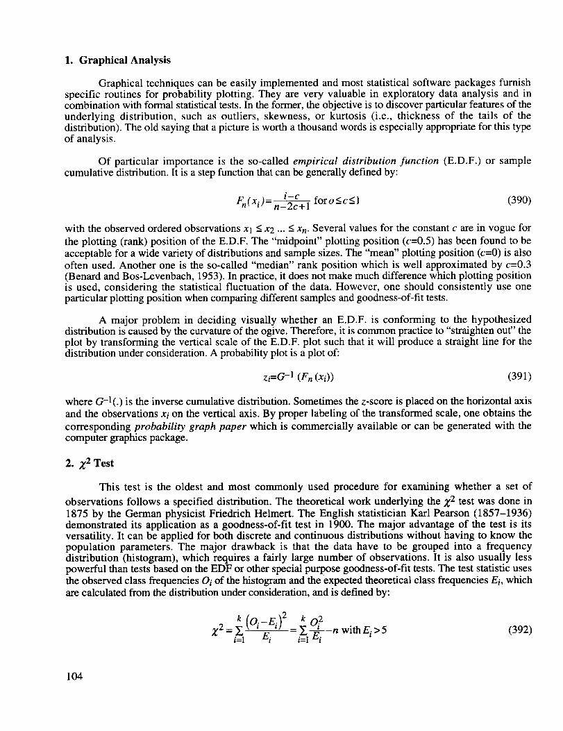
1. Graphical Analysis

Graphical techniques can be easily implemented and most statistical software packages furnishspecific routines for probability plotting. They are very valuable in exploratory data analysis and incombination with formal statistical tests. In the former, the objective is to discover particular features of theunderlying distribution, such as outliers, skewness, or kurtosis (i.e., thickness of the tails of thedistribution). The old saying that a picture is worth a thousand words is especially appropriate for this typeof analysis.

Of particular importance is the so-called empirical distribution function (E.D.F.) or samplecumulative distribution. It is a step function that can be generally defined by:

i--c

Fn(xi)= n--_+l foro<c<l (390)

with the observed ordered observations Xl < x2 ... < Xn. Several values for the constant c are in vogue for

the plotting (rank) position of the E.D.F. The "midpoint" plotting position (c=0.5) has been found to be

acceptable for a wide variety of distributions and sample sizes. The "mean" plotting position (c=0) is alsooften used. Another one is the so-called "median" rank position which is well approximated by c=0.3(Benard and Bos-Levenbach, 1953). In practice, it does not make much difference which plotting positionis used, considering the statistical fluctuation of the data. However, one should consistently use oneparticular plotting position when comparing different samples and goodness-of-fit tests.

A major problem in deciding visually whether an E.D.F. is conforming to the hypothesizeddistribution is caused by the curvature of the ogive. Therefore, it is common practice to "straighten out" theplot by transforming the vertical scale of the E.D.F. plot such that it will produce a straight line for thedistribution under consideration. A probability plot is a plot of:

zi=G -1 (F n (xi)) (391)

where G-l(.) is the inverse cumulative distribution. Sometimes the z-score is placed on the horizontal axis

and the observations xi on the vertical axis. By proper labeling of the transformed scale, one obtains the

corresponding probability graph paper which is commercially available or can be generated with thecomputer graphics package.

2. Z 2 Test

This test is the oldest and most commonly used procedure for examining whether a set of

observations follows a specified distribution. The theoretical work underlying the X2 test was done in

1875 by the German physicist Friedrich Helmert. The English statistician Karl Pearson (1857-1936)demonstrated its application as a goodness-of-fit test in 1900. The major advantage of the test is itsversatility. It can be applied for both discrete and continuous distributions without having to know thepopulation parameters. The major drawback is that the data have to be grouped into a frequencydistribution (histogram), which requires a fairly large number of observations. It is also usually less

powerful than tests based on the EDF or other special purpose goodness-of-fit tests. The test statistic usesthe observed class frequencies Oi of the histogram and the expected theoretical class frequencies Ei, which

are calculated from the distribution under consideration, and is defined by:

2 o:Z2= _ - _,_--n withE i >5

i=l ei i=1/_i(392)

104

where k is the number of class intervals of the histogram and n the total number of observations. Thefollowing constraint exists between the observed and the expected frequencies:

_0 i =_,E i =n. (393)

The sampling distribution of this statistic is approximately the X 2 distribution with degrees of

freedom v=-k- 1 - m where m is the number of population parameters that have to be estimated from the

data. For this approximation to be valid, the number of expected frequencies Ei should be greater than

five. If this number is smaller, then adjacent class intervals can be combined ("pooled"). Class intervals donot have to be of equal size.

The ,,1(2test statistic is intuitively appealing in a sense that it becomes larger with increasing

discrepancy between the observed and the expected frequencies. Obviously, if the discrepancy exceedssome critical value we have to reject the null hypothesis H0 which asserts that the data follow a

hypothesized distribution. Since the alternative hypothesis is not specified, this procedure is also called the

Z 2 test of significance. Typical significance levels are ct=0.10, 0.05, and 0.01. When selecting a

significance level it is important to keep in mind that a low level of significance is associated with a highType II error, i.e., the probability of assuming that the data follow a suggested distribution when they arereally not. Therefore the higher we choose the significance level, the more severe is the test. This aspect ofthe goodness-of-fit test is, at first sight, counterintuitive, because, as was mentioned above, we are usuallyinterested in rejecting the null hypothesis rather than in accepting it.

Table 5 illustrates the procedure of applying the Z 2 test. It shows a table of the observed andexpected frequencies of tossing a die 120 times.

TABLE 5.--Procedure of applying the Z 2 test.

Dieface 1 2 3 4 5 6Observedfrequency 25 17 15 23 24 16Expectedfrequency 20 20 20 20 20 20

The test statistic yields X2=5.00. Since the number of class intervals is 6 and no population

parameter is estimated, the degrees of freedom are v=-6-1=5. If we choose a significance level of t_----0.05

the critical value is Z20.05=11.1. Therefore, we accept the null hypothesis, which means we assume thatthe die is fair.

We must also look with skepticism upon a Z 2 value that is unreasonably close to zero. Because of

the natural statistical fluctuation of the data, we should not expect the agreement between the observed andthe expected frequencies to be too good.

The problem of a small Z 2 value is illustrated by the strange case of monk Gregor Mendel's peas.

Writing in 1936, the famous English statistician R.A. Fisher wondered if, given the statistical fluctuationsof experimental data in the field of genetics (Mendel, 1822-1884), Mendel's results were too good. In

effect, Fisher tested the left-hand side of the Z 2 distribution for a too low Z 2 value. Examining Mendel' s

data conducted over an 8-year interval, he found the Z 2 value to be Z2=41.606 with 84 degrees of

freedom. This corresponds to a level of significance of a=2.86 x 10-5. Therefore one would expect to

105

find suchalow Z 2 value only three times in 100,000 experiments. Perhaps Mendel was deceived by an

overly loyal assistant who knew what results were desired.

It has been said by some critics of the Z 2 test, that it will always reject the null hypothesis if the

sample size is large enough. This must not necessarily be the case.

3. Kolmogorov-Smirnov Test

The Kolmogorov-Smirnov test (see fig. 50) is one of many alternatives to the Z 2 test. The test is

called an E.D.F. test because it compares the empirical distribution function with the theoretical cumulativedistribution. The E.D.F. for this test is defined as:

Fn (xi)=i/n (394)

where the xi's are the ordered n observations. With each increase of an x value, the step function takes a

step of height lln. The test statistic is:

D=max IF n (xi) - F(x) I

If D exceeds a critical value Da, the null hypothesis is rejected.

(395)

F(x)

1

0.90.80.70.60.50.40.30.201

oI L

xl x2 x. x

FIGURE 50.--Kolmogorov-Smirnov test.

The Kolmogorov-Smirnov test can also be used for discrete distributions. However, if one uses the tableswhich assume that the distribution is continuous, the test turns out to be conservative in the sense that if

H0 is rejected, we can have greater confidence in that decision. In cases where the parameters must beestimated, the Kolmogorov-Smirnov test is not applicable. Special tables exist for some particulardistributions such as the exponential and the normal distribution. For a normal distribution for which the

mean and variance have to be estimated, the following asymptotic critical D values (table 6) can be used if

the sample size n > 20.

TABLE 6.--Normal distribution.

0.01 0.05 0.10

Dc 1.031 0.886 0.805

106

OtherE.D.F.statisticsthat measurethe differencebetweenFn (x) and F(x) are found in the literature. A

widely used one is the quadratic statistic:

to

Q=n f {Fn(X)-F(x)}21tt(x)dF(x)--0o

(396)

where _(x) is a suitable weighting function for the squared differences under the integral. When _/t(x)=l,

the statistic is the Cramer von Mises statistic, now usually called W 2, and when _(x)=[F(x){ 1 -F(x)] -1

the statistic is the Anderson-Darling (1954) statistic, called A 2. The E.D.F. test associated with the latter

statistic is recommended in Volume 2 of MIL-HDBK-5F for testing the normality of data.

I. Quality Control

In recent years engineers have witnessed a dramatic revival of interest in the area of statistical

quality control (SQC). One of its new features is a "process orientation" according to which emphasis isshifted towards the improvement of a product during the engineering design and manufacturing phases

rather than attempting to control quality by inspecting a product after it has been manufactured. Time-honored maxims are being quoted and rediscovered. Some of them are: "It is more efficient to do it rightthe first time than to inspect it later." "One should fix processes and not products." "All or no inspection is

optimal." The oldest and most widely known is, of course, that "one cannot inspect quality into aproduct."

In addition, the engineering design phase is being modernized and improved by recognizing theimportance of applying the concepts of experimental design, which had been miserably neglected oroverlooked in the field of engineering in the past. This is now often referred to as off-line quality control.Someone has recently remarked that if engineers would have a better background in engineeringprobability and statistics, it would not have been possible for Professor Genichi Taguchi to dazzle themwith what are essentially elementary and simple concepts in the design of experiments that had beenknown for a long time by practicing statisticians. And last, but not least, a new element has beenintroduced called "the voice of the customer" (VOC), which is the attempt to get some feedback from theconsumer about the product.

SQC centers primarily around three special techniques: (1) determining tolerance limits in thedesign phase, (2) setting up control charts for on-line quality control or statistical process control (SPC),and (3) devising acceptance sampling plans after the product has been manufactured.

1. Acceptance Sampling

Acceptance sampling is designed to draw a statistical inference about the quality of a lot based onthe testing of a few randomly selected parts. While acceptance sampling is usually considered part ofquality control, it is very important to understand that it hardly exercises direct leverage over processcontrol. Because many contracts still contain requirements for submitting acceptance sampling plans, it isdesirable for an engineer to know the basic underlying statistical concepts.

Statistical methods of acceptance sampling are well developed for a variety of sampling proceduressuch as single, multiple, and sequential sampling. A single sampling plan consists of drawing a randomsample and develops criteria for accepting or rejecting the lot. In a multiple sampling plan, the samplingoccurs in several stages. At each stage a decision is made whether to accept or reject the lot or whether to

continue taking another sample. The concept of multiple sampling can be generalized to sequential

107

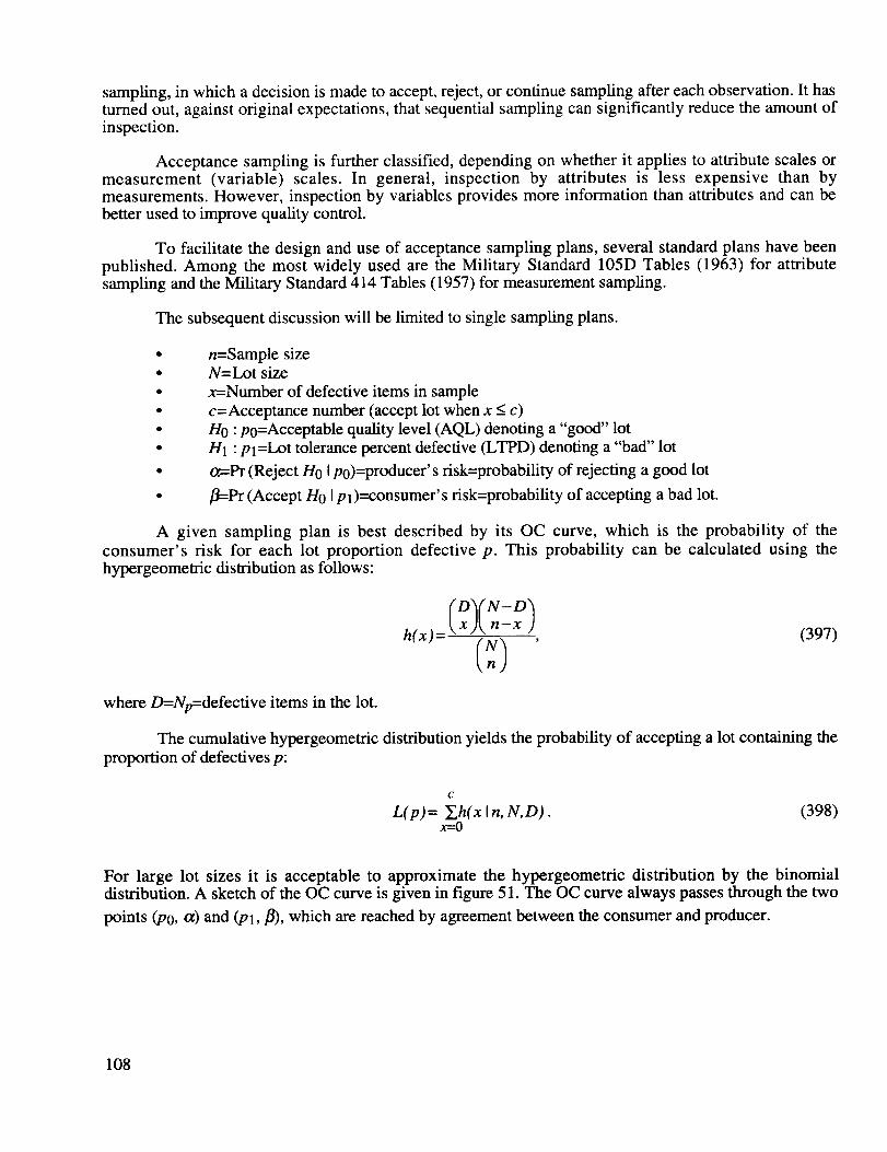
sampling, in which a decision is made to accept, reject, or continue sampling after each observation. It hasturned out, against original expectations, that sequential sampling can significantly reduce the amount of

inspection.

Acceptance sampling is further classified, depending on whether it applies to attribute scales ormeasurement (variable) scales. In general, inspection by attributes is less expensive than bymeasurements. However, inspection by variables provides more information than attributes and can bebetter used to improve quality control.

To facilitate the design and use of acceptance sampling plans, several standard plans have beenpublished. Among the most widely used are the Military Standard 105D Tables (1963) for attributesampling and the Military Standard 414 Tables (1957) for measurement sampling.

The subsequent discussion will be limited to single sampling plans.

n=Sample sizeN=Lot size

x=Number of defective items in sample

c=Acceptance number (accept lot when x < c)H0 : p0=Acceptable quality level (AQL) denoting a "good" lot

HI : pl=LOt tolerance percent defective (LTPD) denoting a "bad" lot

a=Pr (Reject H0 1p0)=producer' s risk=probability of rejecting a good lot

fl=Pr (Accept H0 1pl)=consumer's risk=probability of accepting a bad lot.

A given sampling plan is best described by its OC curve, which is the probability of the

consumer's risk for each lot proportion defective p. This probability can be calculated using thehypergeometric distribution as follows:

(397)

where D=Np=defective items in the lot.

The cumulative hypergeometric distribution yields the probability of accepting a lot containing the

proportion of defectives p:

c

L(p)= _.,h(x In, N,D). (398)x=O

For large lot sizes it is acceptable to approximate the hypergeometric distribution by the binomialdistribution. A sketch of the OC curve is given in figure 51. The OC curve always passes through the two

points (P0, a) and (Pl, fl), which are reached by agreement between the consumer and producer.

108

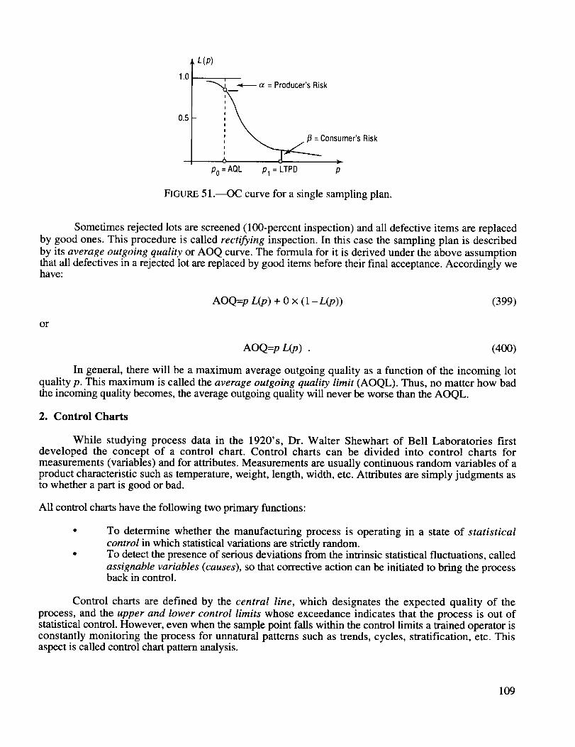
1.0

0.5

L(p)

--- a = Producer'sRisk

- Consumer's Risk

5 _Po=AQL Pl = LTPD p

FIGURE 51.---OC curve for a single sampling plan.

Sometimes rejected lots are screened (100-percent inspection) and all defective items are replaced

by good ones. This procedure is called rectifying inspection. In this case the sampling plan is described

by its average outgoing quality or AOQ curve. The formula for it is derived under the above assumptionthat all defectives in a rejected lot are replaced by good items before their final acceptance. Accordingly wehave:

AOQ=p L(p) + 0 x (1 -L(p)) (399)

or

AOQ=p L(p) . (400)

In general, there will be a maximum average outgoing quality as a function of the incoming lotquality p. This maximum is called the average outgoing quality limit (AOQL). Thus, no matter how badthe incoming quality becomes, the average outgoing quality will never be worse than the AOQL.

2. Control Charts

While studying process data in the 1920's, Dr. Walter Shewhart of Bell Laboratories firstdeveloped the concept of a control chart. Control charts can be divided into control charts formeasurements (variables) and for attributes. Measurements are usually continuous random variables of aproduct characteristic such as temperature, weight, length, width, etc. Attributes are simply judgments asto whether a part is good or bad.

All control charts have the following two primary functions:

To determine whether the manufacturing process is operating in a state of statisticalcontrol in which statistical variations are strictly random.To detect the presence of serious deviations from the intrinsic statistical fluctuations, called

assignable variables (causes), so that corrective action can be initiated to bring the processback in control.

Control charts are defined by the central line, which designates the expected quality of the

process, and the upper and lower control limits whose exceedance indicates that the process is out ofstatistical control. However, even when the sample point falls within the control limits a trained operator isconstantly monitoring the process for unnatural patterns such as trends, cycles, stratification, etc. Thisaspect is called control chart pattern analysis.

109

Thefollowing lists thethreetypesof controlchartsfor measurements:

X"-Chart:

Given:/2,cr CentralLine:/2

UCL: 12+ A cr

LCL: #-A cr

Given: x, s Central Line: x

UCL: x + A1 s

where A=3/wn

k

with x= 1 Y.._. (401)ki=l t

n

LCL: x-A1 s

In on-line quality control, the biased sample standard s is used:

i:Z( xi _ _ )zs=_ n (402)

Typical sample sizes n are 4, 5, 6, or 7. These relatively small sample sizes often come from the

selection of subgroups. The control factor A 1 is obtained from the expected value of the standard deviation

s, which is I.ts=C2 a where:

C2 _ _/_2, where F (x) is the gamma function. (403)

Therefore, the control factor is A 1 =A/c2= 3/(c 2 _).

This and subsequent control factors are calculated under the assumption that the measurementscome from a normal population.

Given: x, R Central Line: x

k

UCL: x+ A2 _ with R=li_IR /..: (404)

LCL: x-A2

110

TherangeR is widely used in quality control because it can be easily obtained if the sample size issmall. However, since R depends only on two observations, namely the maximum and the minimum valueof the sample, it contains less information than the standard deviation. This loss of information is

acceptable for a small sample size. A practical rule is to use the standard deviation s when the sample sizeis larger than 12.

In general, the probability distribution of the range R cannot be expressed in simple explicit form.

For the normal case the first four moments of the distribution of the range R have been extensively

tabulated as a function of the sample size n. For the control charts we need only the mean and standard

deviation of the range R. They are denoted by ].tR=d 2 _ and crR=d 3 or. The above control factor is then

given by A2=A/d2.

R-Chart: (n < 12)

Given: o" Central Line: #R--d2 cr (405)

UCL: D2 cr

LCL: D1 o"

where D2=d2 + 3d3 and Dl=d2- 3d3. (406)

m

Given: R Central Line: R

UCL: D4

LCL: D3 R

where D4=D2/d2=(d2 + 3d3)/d2 and D3=D1/d2=(d2-3d3)/d2.

s-Chart: (n > 12)

Given: cr Central Line:/.ts=C2 0(411)

(407)

(408)

UCL: B2 o"

LCL: B1 o" .

The control factors for this chart are obtained using the mean and standard deviation of the sample

distribution of s which are l.ts=C2 a and Crs=c 3 0 with:

-a /n-1 c 2 (409)c3- \J--h--- 2"

We have, then, B2-c2 + 3c3 and Bl=c2- 3c3. (410)

111

Given: g Central Line:

UCL: B4

LCL: B 3

where B4=B2/c2=(c2 + 3c3)/c2 and B3=Bl/c2=(c2 - 3c3)/c 2. (411)

J. Reliability and Life Testing

In life testing, the random variable under consideration is the time-to-failure of a component. In

fatigue studies, the time-to-failure is measured in the number of cycles to failure and is, therefore, adiscrete random variable.

The probability densityf(t) associated with the time T to failure is called the failure-time density

or life distribution. The probability that the component will fail in the time interval (0, t) is given by thecumulative distribution:

t

P(T <_t) = F(t) = If(x) dr (412)0

which, in this context, is called the unreliability function. The complementary cumulative distribution

defines the probability that the component functions longer than time t or survives at least to time t. It isgiven by:

P(T > t)=R(t)=l - F(t) (413)

This is called the reliability function by engineers and survivorshipfunction by actuaries.

NOTE: From a mathematical viewpoint, reliability is by definition a probability, therefore a numberbetween 0 and 1.

By its very nature reliability theory has its focus in aerospace engineering on the tail area of adistribution, which defines low risk or high reliability systems. Thus the difference among differentreliability models becomes significant only in the tails of the distribution where actual observations aresparse because of limited experimental data. In order to be able to discriminate between competing lifedistribution models, reliability engineers resort to a concept which attempts to differentiate amongdistributions because of physical failure mechanisms, experience, and/or intuition. Such a concept is the

failure rate function which originated in actuary theory and mortality statistics where it is called the force

of mortality. It is also indispensable in the analysis of extreme values where it is known as the intensityfunction.

To define this function, we first determine the conditional probability that a component of "age" t

will fail in the subsequent interval (t, t + At) by defining the following events:

A=lifetime t __T __ t + At (414)

B=lifetime T > t. (415)

112

Notice thattheeventB is the condition that no failure has occurred up to time t; i.e., the component has

age t. In terms of these events the conditional probability is, therefore:

P[A_BI=p[t<T<t+AtlT>t] = P[(t<T<t+At)_(T>t)]P[AIB]= P[B] P[T>t] -AG(t). (416)

The numerator in the above equation is the probability that T lies between t and t+At and the denominator

is the reliability function R(t). The equation can, therefore, be rewritten as:

AG(t)= F(t+At)-F(t)R(t) (417)

The failure rate is defined as the probability of failure in the interval per unit time given that no

failure has occurred before time t. Accordingly, we divide the above equation by At and then take the limit

At _ 0 to arrive at the failure rate function:

Z(t) = F'(t)/R(t) = f (t)/R(t) = f (t)/[1- F(t)]. (418)

This function is also called hazard function, hazard rate, or simply hazard. It is, in a sense, thepropensity of failure as a function of age. The failure rate function contains the same information as the

failure time distribution but it is better suited to formulate reliability models for given sets of experimentaldata.

The difference between the failure time density f(t) and the failure rate function z(t) can be

illustrated by comparing it to human mortality. Theref(t) dt is the probability that a newborn person will

die between age t and t + At, whereas z(t) dt is the probability that a person of age t will die in the

subsequent time interval At.

Some statisticians have been investigating the reciprocal 1/z(t) of the failure rate function, which iscalled Mill's Ratio. It has no application in reliability studies.

Two important relationships exist between the failure rate function and the reliability function.

They can be obtained by the following steps. First using F(t)= 1 -R(t) we obtain by differentiation thatF'(t) = -R'(t).

Therefore:

z(t)= R'(t) dl£nR(t)] (419)R(t) dt

Solving this differential equation for R(t) and subsequently using the relationship f(t)=z(t) R(t)yields:

t t

-Iz(x) dx -Jz(x) dxR(t)=e o and f(t)=z(t)e o (420)

113

ThepropertythatR (oo)=0 requires that the area under the failure rate curve be infinite. This is in

distinction to the failure time density for which the area under its curve is one. Therefore the failure rate

function is not a probability density. Whereas f(t) is the time rate of change of the unconditional failure

probability, z(t) is the time rate of change of the conditional failure probability given that the component

has survived up to time t.

EXAMPLE: The function f( t)=c e -at does not quality as a failure rate function because the area under its

curve is finite. Besides this requirement, the failure rate function has also to be nonnegative. Therefore wehave the two properties of the hazard function:

z(t)>O for allt (421)

andtO

S z (t)dt = to (422)O

1. Life Testing

In life testing, a random sample of n components is selected from a lot and tested under specifiedoperational conditions. Usually the life test is terminated before all units have failed. There are essentially

two types of life tests. The fh'st type is a test that is terminated after the In'st r failures have occurred (r < n)and the test time is random. Data obtained from such a test are called failure censored or type I censored

data. The other more common type test is terminated after a predetermined test time. In this case, thenumber of failures is random. Such data are called time censored or type II censored data. Failure

censoring is more commonly dealt with in the statistical literature because it is easier to treat

mathematically. If the failed units are replaced by new ones, the life test is called a replacement test;otherwise, it is called a nonreplacement test. The unfailed units are variously called survivors, run-outs,

removals, suspensions, or censored units.

In recent years the Weibull distribution has become one of the most popular lifetime distributions.Because it can assume a wide variety of shapes, it is quite versatile. Although there exists a quick andhighly visual graphical estimation technique, the maximum likelihood method is more accurate and lends

itself easily to accommodate censored data.

In the following, we present the maximum likelihood method for estimating the two parameters ofthe Weibull distribution and a BASIC computer program for solving the maximum likelihood equations.

Let the life data consist of n units of which R units have failed at times ti and S units have survived

up to time ts. Assuming a Weibull distribution, the likelihood function is given by:

R s /_L= I-Iot_til3-1e-_f lie -atk . (423)

i=1 k=l

Taking the logarithm of the likelihood function called the log-likelihood function yields:

R R s/_gn L= R gnt_ + R gn fl+(fl-1) _, gnti-ot _,tifl-t_ _,t k

i=1 i=1 k=l(424)

114

Thelocationsof theextremevaluesof the logarithm of a function are identical with those of thefunction itself. This can be shown by using the chain rule as follows:

dgnF(x) dgnF(x)xdF(x)_ 1 dF(x)dx = dF dx -F(x) x dx =0. (425)

Therefore, if the function F(x) remains finite in the interval in which the local extreme values are located,the derivative of the logarithm of the function is zero at the same values of x for which the derivative of thefunction F(x) itself is zero.

The derivatives with respect to the Weibull parameters a and fl are:

c) gn L R(426)

and

OgnL_RRc,l., p l_=l fl s fl )_a a + _" gn ti - Ol ti gnt i + 2_ tk gnt k = 0 . (427)i=1 i k=l

We can eliminate a from the first equation and insert it in the second equation to obtain a single

nonlinear equation in ft. Thus, we have:

Ra= R S (428)

_'# + k___lt#i=

and

_ +i_=lgn ti i_=lt# gn ti +k_=ltflkgn tk _oR S - "

i___=lt/fl +k___lt#

(429)

The second equation can be solved for fl by an iterative method and then be used to solve for a.

It is noteworthy that if there are no suspensions, it takes at least two failure times to be able to

estimate the two Weibull parameters. However, if there are suspensions, only one failure time is sufficientto do this. On the other hand, one cannot obtain the parameters if there are only suspensions and nofailures. That is why one often hears the statement that suspensions are a weak source of information.

The following is a BASIC program using Newton's method to calculate the maximum likelihood

estimators for the Weibull parameters in an iterative manner. This method requires an initial guess for the

shape parameter fl of the Weibull distribution. However, the initial values do not have to be too close to

the actual parameter for the algorithm to converge.

115

WEIMLEDEFDBL A-Z

INPUT"R=",R

DIM STATIC R(R)

FOR I=l TO R:INPUT"TR=", R(I):NEXT I

130 :INPUT "S=",SIF S=0 GOTO 140

INPUT"TS=" ,TS'DIM STATIC S(S)'FOR I=1 TO S:INPUT"TS=", S(I):NEXT I

140 :INPUT "B=",B:J=0

150: H=B*.0001:GOSUB 500D=B:Y=F

B=B+H:GOSUB 500

B=D-H*Y/(F-Y):J=J+ 1

IF ABS((D-B)/D)>.000001 GOTO 150BEEP:BEEP

PRINT"B=";B:PRINT"J=";JA=R/(R 1+S 1):E=A^( -1/B)

PRINT"A=";A:PRINT"E="'EEND

500:RI=0:R2=0:R3=0

FOR I=1 TO R

U=R(I)AB:V=LOG(R(I)):W=U*VR 1=R 1+U:R2=R2+V:R3=R3+W:NEXT IS1=0:$3=0

IF S=0 GOTO 580

S I=S*TSAB:S3=S I*LOG(TS):GOTO 580FOR I=1 TO S

U=S(I)^B:V=LOG(S(I)0:W=U*VS I=S 1 +U:S3=S3+W:NEXT I

580 : F=R/B+R2-R*(R3+S3)/(R 1+S 1)RETURN

2. No-Failure Weibull Model

Sometimes when high reliability items are subjected to a time-censored test, no failures occur at

all. This presents a real dilemma, because the traditional methods for estimating the parameters of adistribution cannot be applied. However, when it is assumed that the exponential model holds, one can

determine an approximate lower (1 - ¢x) confidence limit for the mean life of the component, which is

given as:

> 2T with v= 2 degrees of freedom. (430)

116

2ZHere, T is the fixed accumulated lifetime of the components tested and /1 > Z2 cuts off a right-

hand tail of the Z 2 distribution with 2 degrees of freedom. This distribution is identical to the exponential

distribution f(t)=2 e -t/2. Its critical value can be easily determined to be Z2=-2ln a. If there are n

components, each having a lifetime ti on test, then the accumulated lifetime is:

n

T=i_=lt i . (431)

The lower (1 - a) confidence interval is then given by:

n

Y_ti> i=1

P- -gna " (432)

The upper confidence interval is, of course, infinity.

PROBLEM: A sample of 300 units was placed on life test for 2,000 hours without a failure. Determine anapproximately lower 95-percent confidence limit for its mean life.

SOLUTION:

P=_-.(300)(2' 000) _ 2 _74 = 200, 284 hours. (433)

It is not known whether the approximation of the lower bound is conservative in the sense that theactual confidence is higher than the calculated one. In fact, some practicing statisticians advise againstusing this approximation at all. Admittedly, it is an act of desperation, but it appears to give reasonableresults.

The above method can be extended to the Weibull distribution by making use of the following

relationship: If the failure time T has a Weibull distribution with shape parameter fl and characteristic life

77, then the random variable Y=Tfl has an exponential distribution with mean p=rlfl. To show this, we

apply the Jacobian method, according to which we have:

g(y)= f (t) _---fity=Otfltfl-l e-°g# flt@_ 1 . (434)

Expressing the above equation in terms of the new variable y, we obtain:

g(y) = ore -ay with ]./y = 1 =/_fl . (435)

Thus, if no failures have occurred in a time-censored test and the n components have lifetimes

tl, t2 ... tn, the approximate lower confidence for I.ty is:

117

n

#y=rl3 > i_=lti#- -gnot " (436)

From this we obtain the lower confidence limit for the characteristic life:

1

(437)

Notice that the shape parameter 15 is still unknown and cannot be determined from the existing no-failuredata set. To overcome this obstacle, it has been advocated to use historical failure data from similar

components or from engineering knowledge of the failure physics under consideration to supply the

missing Weibull shape parameter. This method is known as Weibayes analysis because it is regarded asan informal Bayesian procedure.

Sometimes the denominator of the above equation is set equal to one. This corresponds to a

(1 -e -1) or 63.2-percent confidence interval for the lower bound. It has been said that for this condition"the first failure is imminent." This statement must surely rank among the most bizarre ever made in life

testing analysis.

K. Error Propagation Law

Instead of aspiring to calculate the probability distribution of an engineering system response or

performance from the distribution of the component variables (life drivers), it is frequently adequate togenerate some of its lower order moments. It is known, for instance, that the knowledge of the first fourmoments of a distribution enables one to establish a Pearson-type distribution or a generalized lambdadistribution from which percentiles of the distribution can be estimated. Since these two families ofdistributions can accommodate a wide variety of distributions, the technique is often quite effective and theresult is usually better than expected. Generating approximate system performance moments by this

method is generally known as statistical error propagation. Sometimes it is referred to as the Delta

Method or the Root-Sum-Square (RSS) Method.

In order to apply this technique, the functional relationship between the system output(performance) and system parameters (life drivers) must be explicitly known or at least be approximated.The essence of the technique consists in expanding the functional relation in a multivariate Taylor seriesabout the design point or expected value of the system parameters and retaining only lower order terms.The goodness of the approximation depends strongly on the magnitude of the coefficient of variation of thesystem parameter distributions; the smaller the coefficient of variation, the better is the approximation.

The analysis is actually rather straightforward, albeit tedious, for moments higher than the second.A software package called Second Order Error Propagation (SOERP) relieves one of this drudgery.Despite its misleading acronym, it performs higher order error propagation analysis for complicatedengineering systems. The following exposition is limited to calculating only the first two moments, namelythe mean and variance, of a system output.

Let the performance of a system in terms of its system parameters Xl, x2 ... Xn be given by:

z=f(Xl, X 2 ... Xn) (438)

118

Let P=(//1,/22 ... #n) and o'=(al, 0°2... 00n) denote the vector of the mean and standard deviation

of the system parameters, respectively.

The Taylor series expansion of the function z about the point//=(//1,//2 • • • // n) can besymbolically defined by:

z= f(xl,x 2 .... Xn)= _ -_-7,AXl __ +Ax2 _. +...AXn f(xl,x2...Xn) (439)

n=0 n. L UZl az2 n 1121 ,F/2.. "]'/n

where Axi=(xi-//i) and the partial derivatives are evaluated at the design point//=(//1,/1 2 ..... //n).

Retaining only terms up to second order we have:

z=f(//1,//2...//n)+ n (Xi--//i)--Fl-ly,=l_.( c92f (Xi--//i)(Xj--//j).

J=l_ °_i_j

(440)

1. The Mean of the System Performance

To calculate the mean of the system performance we take the expectation of the above equation andobserving that E((Xi-//i))=O, we obtain:

E(z ) = laz = f ( // )+ _.r. .=t_lj=l_ O_XiO_jflu E[(xi -_i ) (Xj --//j )]. (441 )

Deleting the second-order term, we get the fh'st-order approximation for the mean system performance:

E(z)=// z=f (//) . (442)

2. The Variance of the System Performance

The calculation of the variance is more complex than the one of the mean. In fact, the calculationsbecome substantially more lengthy with increasing order of the moments. To begin with, we calculate the

variance for the case of two system parameters x and y. This is not a real loss in generality. Once the resultfor this case has been obtained, the extension to more than two variables can be rather easily recognized.Let the system performance function be given by:

z=f(x, y) (443)

Furthermore, let us denote the variance of a random variable X by V(X)=E(X-E(X))2=E(X -

//x)2=002 and the partial derivative of a function with respect to a variable, say x, byfx.

(a) First-Order Taylor Series Approximation. Here we take only the first terms of the aboveTaylor series. The first-order approximation of the variance of the system performance is then obtained by:

119

2= f x2 o-2 + f y2 o-y + 2 f x f y o-xy

(444)

where o-xy is the covariance of x and y. The partial derivatives fx andfy are sometimes called sensitivitycoefficients.

Recalling that the covariance is related to the correlation coefficient by O'xy=P o-x Cry, we obtain the

standard deviation of the system performance by taking the square root of the above equation:

o-z=\/ f2 o-2 + f2 o-2y+ 2 fx 4 PO-xo-y " (445)

Extension of this expression to more than two system parameters is straightforward. An important,

because often encountered, situation arises if the system parameters are independent (p=0). For this

special case the standard deviation of the system performance simplifies to:

i

= ,,'f2 +fy2o-z \Jx °-2 °'2" (446)

This formula is the reason why this method is also called Root-Sum-Square Method. If correlationis suspected but unknown, one can use the upper limit of the standard deviation which is given by:

o-z< ,fx l o-x+ ,fy l o-y . (447)

This corresponds to a "worst-on-worst" type situation.

Before proceeding to the second-order approximation, we examine some special cases of practicalimportance.

Multi-Output Linear System._=A x_. Let the system performance function be a vector function of

the following form:

(448)

where the system performance (output) vector _ is an (m x 1) vector and the system parameter vector _xbe

an (n x 1) vector. We expand now the system performance function in a Taylor series. Without loss of

generality we set the value of the performance function at the design point equal to zero and obtain thelinearized system performance function as:

y=A x (449)

where A is an (m x n) matrix. It is known as the Jacobian matrix or system sensitivity matrix and its

elements are the first partial derivatives of the system performance vector function tt=f(x).

To calculate the first-order approximation of the system performance variance, we introduce thecovariance matrix which is defined as:

120

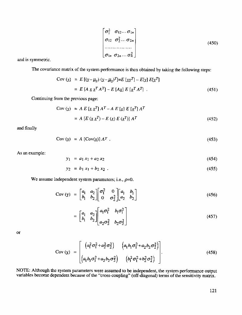
-0"2 0-12... 0-1n"

0-12 0-2 ... 0-2n

O'ln 0-2n ..- 0 -2

and is symmetric.

The covariance matrix of the system performance is then obtained by taking the following steps:

Cov (y_)= E [(Y-Ux) (Y-I_)T] =E [y_yT]_ Ely] E[_T]

= E [A xxTA T]-E [Ax] E [x_TAT] .

Continuing from thepreviouspage:

Coy(y) = AE[x_x_ T]AT-AE[x_]E[x_ T]A T

= A [E (x_x_T)- E (x)E (_xT)]A T

and finally

Coy (y) = A [Cov(x__)]AT

(450)

(451)

(452)

(453)

As an example:

or

Yl = alXl +a2x2

Y2 = bl Xl +b2x2 •

We assume independent system parameters; i.e., p=0.

[a_ °2110-?0 IFa,Cov (x) = L_ _JL0 o==JLaz

a2l[ala? t_0-2]Fa'LOl b2 ][a20"2 b20"2 ]

(454)

(455)

_] (456)

(457)

(a20-2+a20-2) (458)

cov(_) L(a,b,°?+a_b=°_)(b?o?+by0-_)J

NOTE: Although the system parameters were assumed to be independent, the system performance outputvariables become dependent because of the "cross-coupling" (off-diagonal) terms of the sensitivity matrix.

121

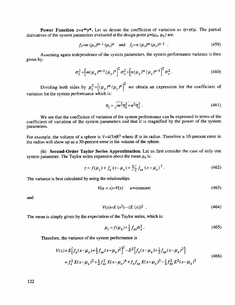
Power Function z=xray n. Let us denote the coefficient of variation as rl=tr/I.t. The partial

derivatives of the system parameters evaluated at the design point kt=(I.tx, _ty) are:

fx=m (/.tx) m-l (l.ty) n and fy=n (lax) m (!Lty)n-1 (459)

Assuming again independence of the system parameters, the system performance variance is then

given by:

l

Dividing both sides by l.t2=[(flx)m(l_y)n] 2 we obtain an expression for the coefficient of

variation for the system performance which is:

7_ ,/_2,,,2 +n2r12 (461)Z -- _,rr,_ _/X

We see that the coefficient of variation of the system performance can be expressed in terms of the

coefficient of variation of the system parameters and that it is magnified by the power of the system

parameters.

For example, the volume of a sphere is V=4/3rcR 3 where R is its radius. Therefore a 10-percent error inthe radius will show up as a 30-percent error in the volume of the sphere.

(b) Second-Order Taylor Series Approximation. Let us first consider the case of only one

system parameter. The Taylor series expansion about the mean #x is:

z = f(_t x ) + fx (x- _x ) + 1/12fxx (x - _tx ) 2 (462)

The variance is best calculated by using the relationships

V(a + x)=V(x) a=constant (463)

and

V(x)=E (x 2) -(E (x)) 2 (464)

The mean is simply given by the expectation of the Taylor series, which is:

#z = f(#x)+ l fxxtr2 . (465)

Therefore, the variance of the system performance is

[ ) ](466)

= f2 E(x-lax_2 + l ¢ 2, ___axxE(x_#x)a+fxfxxE(x_l.tx)3 1 2--_ f_ E2(x-12x )2

122

or

1 F2 rr4 (467)O-z = ax£2Cr2 * lvx-4axxe2 //4 + fxfxx//3 --4axxvx

where//3=skewness and//4=kurtosis of the system parameter.

For example: z=x 2.

We assume the system parameter to be normally distributed with//x=0 and o'2=1. We have the

derivativesfx=2X, fxx=2 and the moments//x=0, o'2=1,//3=0, and//4=3. From this we obtain the mean

and variance of the system performance as

//z=l and 2o-x =2 (468)

It can be shown that these moments agree with the exact moments of the variable z, which in this case has

a Z 2 distribution with 1 degree of freedom.

The case of several parameters becomes more complicated and will not be further pursued. Foruncorrelated system parameters, the resulting expressions for the system performance moments, retainingonly third-order terms in the final result, yield:

n 2Variance: o-2 = i_1_..-/_ o-2(xi)+i_I°3f-°3f_-iilI_-o_x-f.2tl//3(xi) (469)

n 3

Skewness:

Kul"tosis: //4(z)_ (O3f/4 +6_ (°3f/2(°3f 12---- 0 -2 (Xi)O "2 (Xj)

i>j

All derivatives are again evaluated at the design point of the system.

(470)

(471)

123

BIBLIOGRAPHY

Abramowitz, M., and Stegun, A., editors: Handbook of Mathematical Functions. Dover, 1964.

D'Agostino, R.B., and Stephens, M.A., editors: Goodness-of-Fit Methods. Marcel Dekker, New York,NY, 1986.

Freund, J.E., and Walpole, R.E.: Mathematical Statistics. Third Edition, Prentice-Hall, EnglewoodCliffs, NJ, 1980.

Gibra, Isaac N.: Probability and Statistical Inference for Scientists and Engineers. Prentice-Hall,Inc., 1973.

Guttman, I.: Statistical Tolerance Regions: Classical and Bayesian. Hafner, Darien, CN, 1970.

Hahn, G.J., and Shapiro, S.S.: Statistical Models in Engineering. John Wiley & Sons, New York,NY, 1967.

Hall, M.: Combinatorial Analysis. Blaisdell Publishing Co., 1967.

Hampel, F.R.; Ronchetti, E.M.; Rosseeuw, P.J.; and Stahel, W.A.: Robust Statistics: The Approach

Based on Influence Functions. John Wiley & Sons, Inc., New York, NY, 1986.

Hogg, R.V., and Craig, A.T.: Introduction to Mathematical Statistics. MacMillan PublishingCompany, New York, NY, 1978.

Johnson, N.L., and Leone, F.C. Statistics and Experimental Design. John Wiley & Sons, 1964.

Kapur, K.C., and Lamberson, L.R.: Reliability in Engineering Design. John Wiley & Sons, NewYork, NY, 1977.

Kendall, M.G., and Stuart, A.: The Advanced Theory of Statistics. Vol. 1, 4th ed., vol. 2, 4th ed., vol.

3, 4th ed., MacMillan Publishing Company, New York, NY, 1977, 1979, and 1983.

Kennedy, W.J., Jr., and Gentle, J.E.: Statistical Computing. Marcel Dekker, New York, NY, 1980.

Lawless, J.F.: Statistical Models and Methods for Lifetime Data. John Wiley & Sons, New York,NY, 1981.

Meyer, Stuart L.: Data Analysis. John Wiley & Sons, New York, NY, 1975.

MIL-HDBK-5F, vol. 2, 1 November 1990.

Miller, I.R., Freund, J.E., and Johnson, R.: Probability and Statistics for Engineers. Fourth Edition,

Prentice-Hall, Englewood Cliffs, N J, 1990.

Mosteller, F., and Tukey, J.W.: Data Analysis and Regression. Addison-Wesley Publishing Co.,Reading, MA, 1977.

124

Nelson,W.: Applied Life Data Analysis. John Wiley & Sons, New York, NY, 1982.

Scarne, John: Scarne's New Complete Guide to Gambling. Simon and Schuster, 1986.

Shooman, M.L.: Probabilistic Reliability: An Engineering Approach. Second Edition, Robert E.Krieger Publishing Company, Malabar, FA, 1990.

Spiegel, M.R.: Theory and Problems of Statistics. Second edition, Schaum's Outline Series, McGraw-Hill, New York, NY, 1988.

125

REPORT DOCUMENTATION PAGEForm Approved

OMB No. 0704-0188

Public reporting burden for this collection of information is estimated to average 1 hour per response, including the time for reviewing instructions, searching existing data sources,gathering and maintaining the dale needed, and compieUng and reviewing the collection of information. Send comt'nents regarding this burden estimate or any other aspect of thiscolklcticn of information, including suggestions for reducing this burden, to Washington Headquarters Sen,ices, Directorate for Information Operation and Reports, 1215 JeffersonDavis Highway, Suite 1204, Arlington, VA 22202-4302, and to the Office of Management and Budget, Paperwork Reduction Project (0704-0188), Washington, DC 20503

1. AGENCY USE ONLY (Leave Blank) 2. REPORT DATE 3. REPORT TYPE AND DATES COVERED

March 1998 Technical Publication

4. TITLE AND SUBTITLE 5. FUNDING NUMBERS

Probability and Statistics in Aerospace Engineering

6. AUTHORS

M.H. Rheinfurth and L.W. Howell

7. PERFORMINGORGANIZATIONNAMES(S)ANDADDRESS(ES)

George C. Marshall Space Flight Center

Marshall Space Flight Center, Alabama 35812

g. SPONSORING/MONITORINGAGENCYNAME(S)ANDADDRESS(ES)

National Aeronautics and Space Administration

Washington, DC 20546-0001

8. PERFORMING ORGANIZATION

REPORT NUMBER

M-856

10. SPONSORING/MONITORING

AGENCY REPORT NUMBER

NASA/TP-- 1998-207194

11. SUPPLEMENTARY NOTES

Prepared by Systems Analysis and Integration Laboratory,

Science and Engineering Directorate

12a. DISTRIBUTION/AVAILABILITY STATEMENT

Unclassified-Unlimited

Subject Category 65Standard Distribution

12b. DISTRIBUTION CODE

13. ABSTRACT (Maximum200 words)

This monograph was prepared to give the practicing engineer a clear understanding of

probability and statistics with special consideration to problems frequently encountered in

aerospace engineering. It is conceived to be both a desktop reference and a refresher for

aerospace engineers in government and industry. It could also be used as a supplement to

standard texts for in-house training courses on the subject.

14. SUBJECT TERMS

statistics, probability, Bayes' Rule, engineering

17. SECURITY CLASSlRCATION 18. SECURITY CLASSIRCATION

OF REPORT OF THIS PAGE

Unclassified Unclassified

NSN 7540-01-28(_5500

lg. SECURITY CLASBIRCATION

OF ABSTRACT

Unclassified

15. NUMBER OF PAGES

13416. PRICE CODE

A0720. LIMITATION OF ABSTRACT

Unlimited

Standard Form 298 (Ray. 2-89)Prucdl04d by ANSi _d. 230-1829_102

probability and statistics nasa

Documents